
Seven Sisters, East Sussex Beachy Head Lighthouse, East Sussex.

A University of Sussex PhD thesis
Available online via Sussex Research Online:
http://sro.sussex.ac.uk/
This thesis is protected by copyright which belongs to the author.
This thesis cannot be reproduced or quoted extensively from without first obtaining permission in writing from the Author
The content must not be changed in any way or sold commercially in any format or medium without the formal permission of the Author
When referring to this work, full bibliographic details including the author, title, awarding institution and date of the thesis must be given
Please visit Sussex Research Online for more information and further details

Determination of Areas and Basins of Attraction in Planar Dynamical Systemsusing Meshless Collocation
James McMichen
Work submitted in July 2016 in fulfilment of the requirements of a DPhil inMathematics at the University of Sussex

i
UNIVERSITY OF SUSSEXJames McMichen
Thesis submitted in fulfilment of a Dphil in Mathematics
This work is focused on the approximation of sets of attractive solutions of planardynamical systems. Existing work has shown that for many dynamical systems a
Riemannian contraction metric can be used to determine sets of solutions with certainattraction properties. For autonomous dynamical systems in R2 it has been shown that
the Riemannian contraction metric can be reduced to a scalar weight function W . In thiswork we show that a similar result holds true for finite-time dynamical systems with one
spatial dimension. We show how meshless collocation can be used to construct anapproximation of W . The approximated weight function can then be used to determinesubsets of the area of exponential attraction. This is the first time a method has beenintroduced to approximate finite-time areas of exponential attraction. We also give aconvergence proof for the method. For autonomous dynamical systems in R2 there
already exists a method that uses W to determine a subset of the basin of attraction ofan exponentially stable periodic orbit, Ω. However that method relies on properties of Ωbeing known. We show that the existing equation for W can be manipulated so that noknowledge of the periodic orbit is required to approximate W . We present a method thatutilises meshless collocation to approximate W and show that the method is convergent.The approximant of W is then used to determine subsets of the basin of attraction of Ω.
i

ii
Dedication
I would like to give my deepest thanks to my supervisor Peter, without his understanding,patience, kindness and support I would not have finished this work . I would also like tothank my partner Mel for her tireless support. Finally I’d like to thank my internal andexternal examiners for their feedback regarding the original submission.
ii

CONTENTS iii CONTENTS
Contents
1 Introduction 21.1 Overview . . . . . . . . . . . . . . . . . . . . . . . . . . . . . . . . . . . . . 21.2 State of the Art . . . . . . . . . . . . . . . . . . . . . . . . . . . . . . . . . . 4
1.2.1 Finite-Time Dynamical Systems . . . . . . . . . . . . . . . . . . . . 41.2.2 Borg’s Criterion and Approximation of the Basin of Attraction of
Periodic Orbits . . . . . . . . . . . . . . . . . . . . . . . . . . . . . . 7
2 Meshfree Collocation Applied to Dynamical Systems, using Radial BasisFunctions (RBF) 92.1 Introduction . . . . . . . . . . . . . . . . . . . . . . . . . . . . . . . . . . . . 92.2 Interpolation . . . . . . . . . . . . . . . . . . . . . . . . . . . . . . . . . . . 102.3 Generalised Interpolation . . . . . . . . . . . . . . . . . . . . . . . . . . . . 112.4 Mixed Interpolation . . . . . . . . . . . . . . . . . . . . . . . . . . . . . . . 132.5 Wendland Functions . . . . . . . . . . . . . . . . . . . . . . . . . . . . . . . 142.6 Introduction to Dynamical Systems . . . . . . . . . . . . . . . . . . . . . . . 162.7 Example . . . . . . . . . . . . . . . . . . . . . . . . . . . . . . . . . . . . . . 192.8 Error Estimates . . . . . . . . . . . . . . . . . . . . . . . . . . . . . . . . . . 202.9 Literature Review of Meshless Collocation and Dynamical Systems . . . . . 23
3 Approximating the area of exponential attraction of finite-time dynam-ical systems in R 253.1 Introduction . . . . . . . . . . . . . . . . . . . . . . . . . . . . . . . . . . . . 253.2 Theoretical Foundations . . . . . . . . . . . . . . . . . . . . . . . . . . . . . 26
3.2.1 Preliminaries . . . . . . . . . . . . . . . . . . . . . . . . . . . . . . . 273.3 An Approximant for W . . . . . . . . . . . . . . . . . . . . . . . . . . . . . 35
3.3.1 Meshfree Collocation . . . . . . . . . . . . . . . . . . . . . . . . . . . 383.3.2 Error Analysis . . . . . . . . . . . . . . . . . . . . . . . . . . . . . . 42
3.4 Examples . . . . . . . . . . . . . . . . . . . . . . . . . . . . . . . . . . . . . 463.4.1 Analytically Solvable System . . . . . . . . . . . . . . . . . . . . . . 463.4.2 Nonautonomous Example . . . . . . . . . . . . . . . . . . . . . . . . 49
4 Approximating the basin of attraction of a periodic orbit in two dimen-sions 534.1 Introduction . . . . . . . . . . . . . . . . . . . . . . . . . . . . . . . . . . . . 534.2 Theoretical Foundations . . . . . . . . . . . . . . . . . . . . . . . . . . . . . 54
4.2.1 Sufficiency . . . . . . . . . . . . . . . . . . . . . . . . . . . . . . . . . 554.2.2 Existence of W . . . . . . . . . . . . . . . . . . . . . . . . . . . . . . 68
4.3 Approximating W . . . . . . . . . . . . . . . . . . . . . . . . . . . . . . . . 764.3.1 Building an Approximation to W . . . . . . . . . . . . . . . . . . . . 79
4.4 Error Analysis . . . . . . . . . . . . . . . . . . . . . . . . . . . . . . . . . . 834.5 Examples . . . . . . . . . . . . . . . . . . . . . . . . . . . . . . . . . . . . . 90
iii

CONTENTS 1 CONTENTS
4.5.1 Analytic Example . . . . . . . . . . . . . . . . . . . . . . . . . . . . 904.5.2 Numerically based Example . . . . . . . . . . . . . . . . . . . . . . . 93
4.6 Appendix: Determining a Positively Invariant Set . . . . . . . . . . . . . . . 97
5 Discussion 99
1

2 CHAPTER 1. INTRODUCTION
Chapter 1
Introduction
1.1 Overview
In this work we are interested in approximating sets of attractive solutions for planar dy-
namical systems. Attractive sets have long been a focus in dynamical systems. Lyapunov
methods tend to be the dominant method for determining attractive sets in this setting.
But over the past 10 years there has been a growing focus on using a local contraction
metric to determine sets of attractive solutions. In this work we build upon these re-
sults. When restricted to planar systems the contraction property can be characterised
by a scalar weight function W . We derive a partial differential equation with W as a
solution. However these differential equations contain an unknown constant. By isolating
the constant and taking the orbital derivative we obtain an equation where W is the only
unknown. We present a methodology to numerically solve these equations via meshless
collocation and show that the method is convergent. We then present numerical examples.
The first planar system we work with is on a finite-time interval with one spatial dimension.
Finite-time dynamical systems are a recent yet rapidly growing area of study. In this work
we use the local contraction property to derive a method of approximating subsets of the
area of exponential attraction for nonautonomous finite-time differential equations. The
area of exponential attraction is a relatively new concept. We show that for finite-time
dynamical systems, a Riemannian contraction metric can be reduced to a scalar weight
function. We derive a differential equation where the orbital derivative of W is the only
unknown. We then present a method that numerically solves this equation using meshless
2

1.1. OVERVIEW 3 CHAPTER 1. INTRODUCTION
collocation and show that the method is convergent. This work adds to existing work
of [Giesl, 2012] which uses Lyapunov functions to construct a subset of the domain of
attraction of a solution. However that method is unable to determine whether a small
neighbourhood of the solution is attractive. Our method does not have this limitation so
can be used to fill in this missing information. It can also work on sets that either do not
contain an equilibrium, or where it is not known if there is one. Areas of further study
could extend this work to higher dimensions. The main contribution of this chapter is the
introduction of a convergent method to approximate the area of exponential attraction.
The second planar system we work with is an autonomous differential equation in R2. In
this case we are interested in determining the basin of attraction of a periodic orbit, Ω.
We build upon a method developed in [Giesl, 2007b] that used scalar weight functions to
approximate the basin of attraction of Ω. However that method requires properties of Ω
to be known a-priori. The method we present does not need any information about Ω to
be implemented. We a present a convergent method to approximate the weight function
which can then be used to approximate the basin of attraction of a periodic orbit. The
natural evolution for this method is to be extended into higher dimensions.
This work is structured as follows. In Section 1.2 we review the existing literature for finite-
time dynamical systems and generalisations of Borg’s criterion and the determination of
the basin of attraction for periodic orbits.
Chapter 2 gives an introduction to meshless collocation, the method we use to numerically
solve the partial differential equations. In Section 2.2 we show how it can be used to
interpolate function values. This is extended in Sections 2.3 and 2.4 when we look at
generalised and mixed interpolation respectively. In Section 2.5 we present the Wendland
functions, a compactly supported radial basis function that we use in this work. Section
2.6 provides a brief overview of the basics of dynamical systems and then Section 2.7 gives
an example of meshless collocation being used to solve a differential equation involving
the orbital derivative. Then in Section 2.8 we give an overview of how the error estimates
of the method are derived. Finally Section 2.9 reviews the existing literature that applies
meshless collocation to dynamical systems.
3

1.2. STATE OF THE ART 4 CHAPTER 1. INTRODUCTION
In Chapter 3 we present our method for determining the area of exponential attraction for
finite-time differential equations in one spatial dimension. In Section 3.2 we present some
existing work on finite-time dynamics. We then go on to present a new result, in which
we show how to derive a differential equation that can be used to approximate a scalar
weight function, which can then be used to determine areas of exponential attraction. In
Section 3.3 we show how the constant can be eliminated from the differential equation
we derived in the previous section and prove that this new function can still be used to
determine an area of exponential attraction. We then show how meshless collocation can
be used to numerically solve the equation. In Section 3.3.2 we show that our method is
convergent. Finally we close by demonstrating how the method works with two examples.
In Chapter 4 we present a method to determine the basin of attraction of a periodic orbit
in R2. Section 4.2 reviews existing results in the field. In Section 4.3 we derive a differential
equation for the weight function that does not contain any extra unknown variables and
show how this can be numerically solved by meshless collocation. In Section 4.4 we show
that the method is convergent and in Section 4.5 we apply the method to two examples.
We then end the work by drawing some concluding remarks in the discussion.
Throughout this work when the notation ‖ · ‖ is used it denotes the Euclidean norm.
1.2 State of the Art
We present an overview of existing research relating to the main areas this thesis covers:
finite-time dynamical systems, Borg’s criterion and the basin of attraction of periodic
orbits. A literature review of meshless collocation in dynamical systems is given at the
end of Chapter 2.
1.2.1 Finite-Time Dynamical Systems
Finite-time dynamical systems are a relatively new area of study. Despite many appli-
cations focusing on the behaviour of dynamical systems over a finite-time interval, there
was not, until recently, an established theoretical framework for finite-time dynamics in
the way there was for the classical asymptotic systems. In the early 2000s a mathematical
theory of finite-time dynamics was introduced to help in the applications of fluid dynamics
4

1.2. STATE OF THE ART 5 CHAPTER 1. INTRODUCTION
and oceanography. The Lagrangian coherent structure (LCS) was first defined in [Haller,
2000]. An LCS is a manifold in a finite-time dynamical system. It describes a surface of
trajectories that have a dominant influence on nearby trajectories and creates a coherent
trajectory pattern. They can therefore be used to characterise attracting and repelling
material surfaces. Along with the work on LCSs various diagnostic quantities were devel-
oped, such as finite-time Lyapunov exponents (FTLE), finite-time hyperbolicity and the
finite-time spectrum. LCSs are a young but very active area of research and dominant in
the field of finite-time dynamics. A brief review of LCSs can be found in [Peacock and
Dabiri, 2010].
Since they were first defined, there has been active development of the theoretical concepts
concerning LCSs, their detection, and the determination and classification of the type of
trajectories they contain, e.g. hyperbolic, elliptic. The original work was built upon
in [Haller, 2001] where existence criteria for LCSs in three dimensions were given. The
n-dimensional case was then discussed in [Lekienand et al., 2007].
The concept of FTLEs is similar to that of the rate of exponential attraction, that is
defined and studied in Chapter 3, except rather than being restricted to the behaviour of
trajectories at the end time they vary throughout the time domain. A lot of the early work
by Haller introducing LCSs also developed the theory of FTLEs. Further developments
include [Shadden et al., 2005] which developed stronger links between the concepts of
the LCSs and FTLEs and showed that through this link LCSs can be thought of as an
invariant manifold and serve as boundaries of attractive areas. The link between certain
FTLEs and hyperbolic LCSs is given in a rigorous mathematical framework in [Karrasch
and Haller, 2013].
Another important tool in the field of finite-time dynamics and its application to fluid
dynamics and oceanography is that of finite-time hyperbolicity, which originates from
[Haller, 2000]. The classical definition is that a solution is hyperbolic if its linearisation
has an exponential dichotomy, see [Katok and Hasselblatt, 1997]. The finite-time version
of hyperbolicity is very similar and is defined in [Berger, 2011]. That paper goes on to
provide a condition for finite-time hyperbolicity which can be used to show the existence
of invariant manifolds. This is extended in [Berger, 2010], which shows that finite-time
5

1.2. STATE OF THE ART 6 CHAPTER 1. INTRODUCTION
hyperbolicity persists under small continuous perturbations. In [Duc and Siegmund, 2008]
hyperbolicity and invariant manifolds are extended to 2-dimensional finite-time dynamical
systems. Furthermore it gives definitions of finite-time stable and unstable manifolds.
[Duc and Siegmund, 2011] builds upon the existing theories of hyperbolicity and applies
them to a planar Hamiltonian flow. In [Berger et al., 2008] the authors partition the
phase space into attracting, repelling, elliptic and hyperbolic regions and show that in the
case of a linear system with constant coefficients this definition reduces to the traditional
asymptotic definition. A unified theory of finite-time hyperbolicity is presented in [Doan
et al., 2012]. This helps to unify existing theories of FTLEs and different theories of
finite-time hyperbolicity that were introduced in [Rasmussen, 2010] and [Berger et al.,
2009].
In [Rasmussen, 2007] weaker concepts of attraction in finite-time are introduced. The
author then further develops these in [Rasmussen, 2010]. In that work a definition of
attraction is given that allows for trajectories to not be attractive at every point, this differs
to the concept of attractivity that comes out of the LCS school. It also introduces a finite-
time version of the exponential dichotomy that leads to a finite-time spectrum, this differs
from the finite-time spectrum given in [Berger et al., 2009]. Finally it also introduces a
theory of finite-time bifurcation. The weaker concepts of finite-time attractivity are further
extended in [Giesl and Rasmussen, 2012] where they are used to characterise finite-time
areas of (exponential) attraction and domains of attraction of a solution. The work in
Chapter 3 presents a method to approximate areas of exponential attraction via meshless
collocation. Furthermore, [Giesl and Rasmussen, 2012] also introduces a finite-time Borg
criterion and finite-time Lyapunov functions. Domains of attraction of a solution are
approximated via finite-time Lyapunov functions and meshless collocation in [Giesl, 2012].
Finite-time dynamics are starting to move into a varied number of systems. In [Nersesov
and Haddad, 2008] concepts of finite-time stability are extended to impulsive systems
and [Kanno and Uchida, 2014] extends the FTLE theory into time-delayed systems.
6

1.2. STATE OF THE ART 7 CHAPTER 1. INTRODUCTION
1.2.2 Borg’s Criterion and Approximation of the Basin of Attraction of
Periodic Orbits
We consider the autonomous ordinary differential equation
x = f(x), (1.1)
with x ∈ Rn and f ∈ Cσ(Rn,Rn) with σ ≥ 1. Then Borg’s criterion (Theorem 1.2.1) is a
local contraction property first shown in [Borg, 1960].
Theorem 1.2.1. Let ∅ 6= K ⊂ Rn be a compact, connected and positively invariant set
which contains no equilibrium. Moreover assume L(p) < 0 for all p ∈ K where
L(p) := max‖v‖=1,v⊥f(p)
L(p, v),
L(p, v) :=〈Df(p)v, v〉.
Then there exists one and only one periodic orbit Ω ⊂ K, which is exponentially stable.
Moreover its basin of attraction A(Ω) contains K.
The theorem shows that if the distance between trajectories is decreasing at all points
of their orbits then it is a sufficient condition for a periodic orbit to exist. However
if trajectories increase their distance between each other for part of their orbit but then
reduce it by an even greater amount on other parts there will still be a periodic orbit in K,
these types of trajectories will be missed by the original Borg’s criterion. Borg’s criterion
was generalised so that it incorporates a Riemannian contraction metric. This allows for
local trajectories to increase in distance for part of their orbits as long as that increase
is made up for by greater contraction at other parts of their orbits. This was first shown
in [Stenstrom, 1962], where Borg’s criterion was extended to include Riemannian metrics
on Riemannian manifolds, for both equilibrium points and periodic orbits. However Rn was
treated as a special case in which the Riemannian metric becomes constant. In [Hartman
and Olech, 1962] it is generalised by an integral function along the orbit, however this
method was not computable. A similar method was used in [Leonov et al., 1995] to study
the stability and instability of solutions, that are not necessarily periodic, by means of
a linearisation that measures the distance between neighbouring trajectories on a linear
area element transversal to one of the trajectories. In [Leonov et al., 2001] sufficient
7

1.2. STATE OF THE ART 8 CHAPTER 1. INTRODUCTION
conditions for the stability of differential equations on a Riemannian manifold are given
by using a Lyapunov-type function and singular values. It is shown in [Giesl, 2004a]
that a Borg function which is generalised with a Riemannian contraction metric is both
a sufficient and necessary condition for the existence of a unique exponentially stable
periodic orbit in a compact set. This result is then extended to determine the limit cycles
for periodic differential equations in [Giesl, 2004b], non smooth systems in [Giesl, 2005]
and almost periodic differential equations in [Giesl and Rasmussen, 2008]. [Giesl, 2015]
extends the Riemannian contraction metric to work with an equilibrium point and shows
it is a necessary and sufficient condition for a point to be exponentially stable and gives
converse theorems that can aid in the construction of the metric.
In [Giesl, 2007b] a method to approximate the basin of attraction via meshless collocation
is given, we extend this work in Chapter 4, where a deeper analysis is presented. This
method was then extended to higher dimensions [Giesl, 2009] where the local contraction
metric method is used in the neighbourhood of the periodic orbit and a Lyapunov function
is used to determine attractivity outside that neighbourhood. In [Giesl and Hafstein,
2013] a method for approximating the basin of attraction of a periodic orbit for periodic
differential equations in Rn is given. They show that a Riemannian metric can be used
to construct a symmetric matrix. That matrix being negative definite is a sufficient and
necessary condition to characterise the basin of attraction. They use continuous piecewise
affine functions to construct a Riemannian contraction metric and hence approximate the
basin of attraction.
8
9 CHAPTER 2. RBF
Chapter 2
Meshfree Collocation Applied to
Dynamical Systems, using Radial
Basis Functions (RBF)
2.1 Introduction
In both Chapters 3 and 4 of this work we use a specialised Borg criterion to approximate
areas and basins of attraction. In both cases we derive a linear partial differential equation
that cannot usually be solved analytically. The method we present to solve these equations
numerically is meshless collocation. In particular we use radial basis functions. They
have two main advantages. Firstly they are a meshfree method, this means there are no
requirements on mesh triangulation. This allows grid points to be added easily wherever
a finer granularity of data points is required. Secondly their error estimates are given in
terms of the differential operator which aid the construction of error bounds.
In this chapter we give an overview of the methodology. Section 2.2 starts by describ-
ing how the technique is used to interpolate functions. This was how the methodology
was originally employed. In Section 2.3 we describe its use to solve linear differential
equations, this is the method that is most utilised in this work. In Section 2.4 we show
how meshless collocation is used to solve a boundary value problem. We introduce the
Wendland functions in Section 2.5, they are a compactly supported radial basis functions
that we exclusively use in our numerical examples. Some background information about
9

2.2. INTERPOLATION 10 CHAPTER 2. RBF
dynamical systems is given in Section 2.6. An example of generalised interpolation applied
to the orbital derivative is given in Section 2.7. In Section 2.8 we introduce the native
space and describe how the error bounds are obtained. Finally in Section 2.9 we look
at how meshless collocation has been used in the literature to approximate properties of
dynamical systems. The work in this chapter is a brief introduction to the subject. For a
more in depth analysis of radial basis functions we point the reader towards [Wendland,
2005] and [Buhmann, 2003]. For a deeper look at the use of radial basis functions in the
construction of Lyapunov functions we suggest the book [Giesl, 2007a]. For a recent review
of the computational approximation of Lyapunov functions see [Giesl and Hafstein, 2015].
2.2 Interpolation
Radial basis functions were traditionally used for scattered data approximation via func-
tion interpolation, examples of their use include surface reconstruction [Carr et al., 2001]
and image compression [Boopathi and Arockiasamy, 2012]. In our study of radial basis
functions we limit ourselves to functions that are positive definite, there are others such
as conditionally positive definite functions. For more details on this please see [Wendland,
2005]. A function Ψ : Rn → R is called radial if a function ψ : R+0 → R exists such
that Ψ(x) = ψ(‖x‖). We now give a definition of a positive definite function, this is an
important property of radial basis functions as it shows that matrices formed from them
are positive definite and therefore invertible.
Definition 2.2.1. A continuous function Ψ : Rn → R is called positive-definite if for all
N ∈ N, all sets of pairwise distinct centres X = x1, ..., xN with each xi ∈ Rn, and all
α ∈ RN\0
N∑j=1
N∑k=1
αjαkΨ(xj − xk) > 0,
i.e. the quadratic form is positive.
There are many examples of radial basis functions such as the Gaussians, multi-quadric
and thin-plate splines. However we limit our focus to the compactly supported Wendland
functions that were introduced in [Wendland, 1998]. These functions have compact sup-
port which means their interpolation matrices are sparse and therefore more numerically
10
2.3. GENERALISED INTERPOLATION 11 CHAPTER 2. RBF
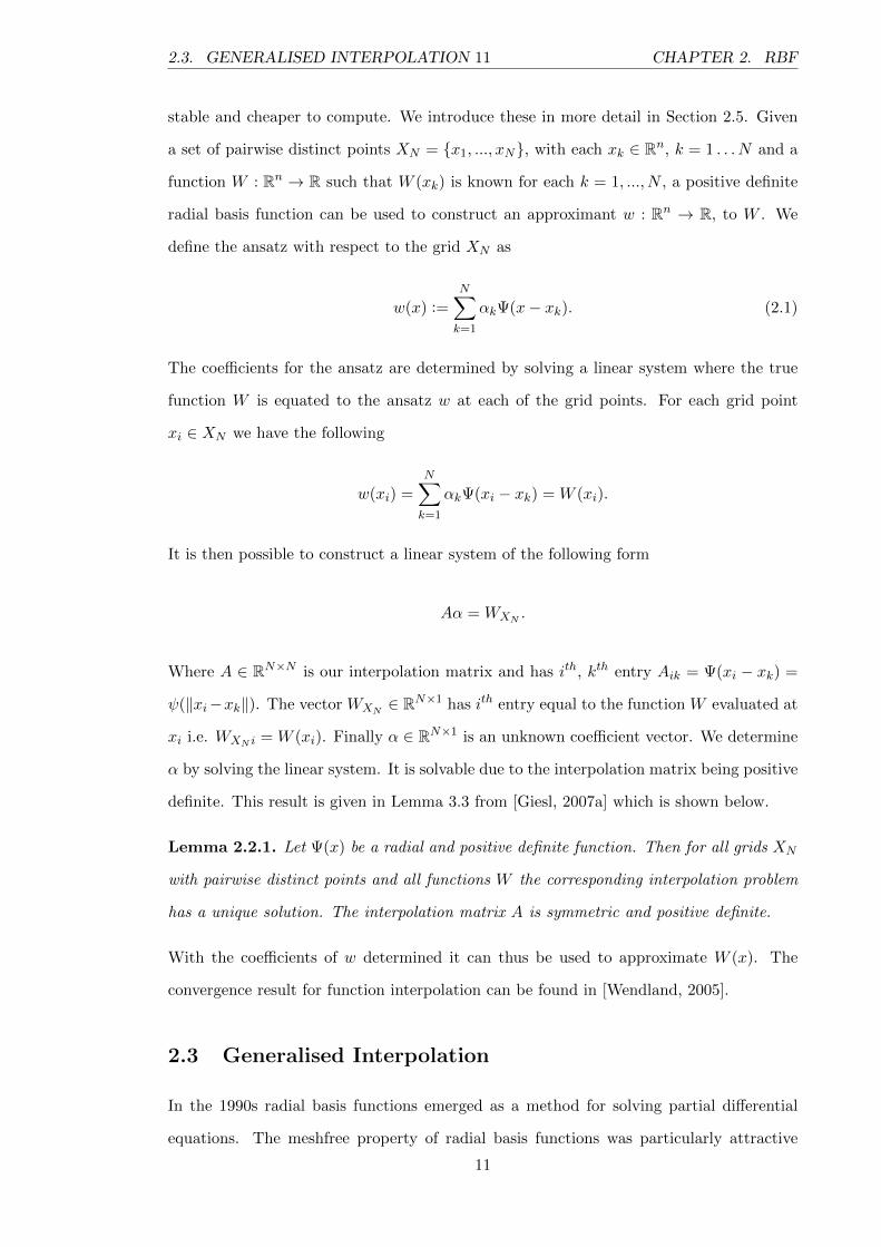
stable and cheaper to compute. We introduce these in more detail in Section 2.5. Given
a set of pairwise distinct points XN = x1, ..., xN, with each xk ∈ Rn, k = 1 . . . N and a
function W : Rn → R such that W (xk) is known for each k = 1, ..., N , a positive definite
radial basis function can be used to construct an approximant w : Rn → R, to W . We
define the ansatz with respect to the grid XN as
w(x) :=N∑k=1
αkΨ(x− xk). (2.1)
The coefficients for the ansatz are determined by solving a linear system where the true
function W is equated to the ansatz w at each of the grid points. For each grid point
xi ∈ XN we have the following
w(xi) =N∑k=1
αkΨ(xi − xk) = W (xi).
It is then possible to construct a linear system of the following form
Aα = WXN .
Where A ∈ RN×N is our interpolation matrix and has ith, kth entry Aik = Ψ(xi − xk) =
ψ(‖xi−xk‖). The vector WXN ∈ RN×1 has ith entry equal to the function W evaluated at
xi i.e. WXN i = W (xi). Finally α ∈ RN×1 is an unknown coefficient vector. We determine
α by solving the linear system. It is solvable due to the interpolation matrix being positive
definite. This result is given in Lemma 3.3 from [Giesl, 2007a] which is shown below.
Lemma 2.2.1. Let Ψ(x) be a radial and positive definite function. Then for all grids XN
with pairwise distinct points and all functions W the corresponding interpolation problem
has a unique solution. The interpolation matrix A is symmetric and positive definite.
With the coefficients of w determined it can thus be used to approximate W (x). The
convergence result for function interpolation can be found in [Wendland, 2005].
2.3 Generalised Interpolation
In the 1990s radial basis functions emerged as a method for solving partial differential
equations. The meshfree property of radial basis functions was particularly attractive
11

2.3. GENERALISED INTERPOLATION 12 CHAPTER 2. RBF
in this field where the incumbent methods such as finite differences and finite elements
required the building of grids that complied to strict rules that made them more difficult to
apply to unusual domains or geometries and expensive to refine. The initial advancement
in the field was made by Kansa in [Kansa, 1990a] and developed in [Kansa, 1990b] where
he applied the method to an elliptic, parabolic and hyperbolic Poisson problem. The
method Kansa introduced has become known as unsymmetric collocation, this is because
when the differential operator is applied to the ansatz the interpolation matrix is usually
not symmetric and not guaranteed to be invertible. This method has been widely used in
applications such as solving the shallow water equations on the sphere [Flyer and Wright,
2009]. Later in the 1990s a number of papers examined Hermite-Birkhoff interpolation
using radial basis functions [Narcowich and Ward, 1994], [Iske, 1995] , [Sun, 1994] and [Wu,
1992], this was the introduction of what is now known as symmetric collocation. In
symmetric collocation the differential operator is applied in the construction of the ansatz
before it is then again applied to the ansatz. This leads to a doubling of the order of
the number of derivatives that need to be calculated in the collocation matrix but comes
with the advantage that the matrix is symmetric. Symmetric collocation has been applied
to a wide variety of problems such as Darcy’s problem [Schrader and Wendland, 2011]
and solving reaction diffusion problems on the surface of the sphere [Wendland, 2013]. A
comparison of the two methods can be found in [Power and Barraco, 2002].
In this section we are interested in showing how radial basis functions can be used in
symmetric collocation to give a solution to a linear partial differential equation of the
form
DW = f on Ω, (2.2)
where Ω is a domain in Rn and D is a general linear operator of the form
DW (x) =∑|α|≤m
cα(x)DαW (x), (2.3)
where the coefficients have a certain smoothness, cα ∈ Cσ(Ω,R) and m,σ ∈ N. Let XN
be a set of pairwise distinct points XN = x1, ..., xN ⊂ Rn where the value DW (xk) is
known for all xk ∈ XN . We introduce Dirac’s δ-operator, which is a pointwise operator, i.e.
12

2.4. MIXED INTERPOLATION 13 CHAPTER 2. RBF
δxkW (x) = W (xk). The following notation is used throughout this work (δxk D)xW (x) =
DW (xk), where the superscript x shows that the operator is to be applied with respect to
the variable x. The reconstruction w of W with respect to the grid XN and the operator
D uses the following ansatz
w(x) =N∑k=1
αk(δxk D)yΨ(x− y).
We determine the coefficient vector by solving a linear system where we equate Dw(xi) =
DW (xi) for each xi ∈ XN . This gives the following system
Aα = WD,XN , (2.4)
where α ∈ RN×1 is the coefficient vector which is to be determined by solving the linear
system and WD,XN ∈ RN×1 is vector where the ith entry is given by WD,XN ,i = DW (xi) =
f(xi). Here A ∈ RN×N is our collocation matrix, it is positive definite under mild condi-
tions on the points XN and Ψ. The matrix has the following form
A =
(δx1 D)x(δx1 D)y · · · (δx1 D)x(δxN D)y
.... . .
...
(δxN D)x(δx1 D)y · · · (δxN D)x(δxN D)y
Ψ(x− y).
Once α has been determined by solving the system (2.4) one can approximate W (x) with
w(x) and DW (x) with Dw(x). We discuss the convergence of this method in Section 2.8.
2.4 Mixed Interpolation
In Chapter 3 the partial differential equation we need to solve is a Dirichlet boundary
problem. This requires both generalised interpolation for the interior points and interpo-
lation for the boundary points. We now describe this method. Consider a boundary value
problem
DW = f on Ω,
W = g on Γ. (2.5)
13

2.5. WENDLAND FUNCTIONS 14 CHAPTER 2. RBF
With Ω a domain in Rn and Γ ⊂ ∂Ω i.e. Γ is a part of the boundary of Ω. D is of the
same form as (2.3). Consider a set of pairwise distinct points XN = x1, . . . , xN with
XN ⊂ Ω and a set of pairwise distinct points on the boundary XΓ = η1, . . . , ηM with
XΓ ⊂ Γ. Then the ansatz to approximate W of (2.5) with respect to the grid XN ∪XΓ is
given by
w(x) =N∑k=1
αk(δxk D)yΨ(x− y) +M∑k=1
βk(δηk)yΨ(x− y).
Then by equating Dw(xi) = f(xi) for each xi ∈ XN and w(ηi) = g(ηi) for each ηi ∈ XΓ we
construct the following collocation system which can be solved to determine the coefficient
vectors αi and βi A C
CT B
α
β
=
F
G
. (2.6)
With the following entries
A ∈ RN×N with the ith, kth entry aik = (δxi D)x(δxk D)yΨ(x− y)
C ∈ RN×M with the ith, kth entry cik = (δxi D)x(δηk)yΨ(x− y),
B ∈ RM×M with the ith, kth entry bik = (δηi)x(δηk)yΨ(x− y) = Ψ(ηi − ηk),
α ∈ RN×1 with ith entry αi,
β ∈ RM×1 with ith entry βi,
F ∈ RN×1 with ith entry Fi = f(xi),
G ∈ RM×1 with ith entry Gi = g(xi).
It is shown in Proposition 3.29 of [Giesl, 2007a] that a special case of the matrix
A C
CT B
is positive definite, hence the system is solvable. Further, as long as a sufficiently small
grid is used w will be a good approximation of W .
2.5 Wendland Functions
In this work we use Wendland functions as our radial basis function. Wendland functions
are piece-wise polynomial compactly supported functions. To see their derivation we point
the reader to [Wendland, 1998]. The Wendland functions are supported on the range
[0, 1], but it is possible to scale the support radius so that it is either larger or smaller. A
14

2.5. WENDLAND FUNCTIONS 15 CHAPTER 2. RBF
smaller support radius leads to the interpolation matrix being sparser and results in better
computational efficiency and numerical stability. However if the support is too small,
relative to the fill distance and the problem being interpolated, then the approximation will
not be good. Hence there is a trade off between computational complexity and accuracy
that needs to be balanced through the choice of the support radius and the grid used for
the approximation. Before defining the Wendland function we introduce a few points of
notation. Let x be a real number. Then the truncated function (x)+ is defined to be zero,
if x < 0 and x otherwise. The floor function bxc gives the largest integer i with i ≤ x. We
define the Wendland functions by
Definition 2.5.1. (Wendland functions). Let n ∈ N and k ∈ N0. We define the Wendland
functions by
ψd,k := Ikψbn2 c+k+1, (2.7)
where ψl := (1− r)l+ and (Iψ)(r) =
∫ ∞r
tψ(t)dt for all r ∈ R+0 .
Table 2.1 shows some examples of Wendland functions for different spatial dimensions.
The table comes from [Wendland, 2005]. The notation.= denotes equality up to a positive
constant factor.
Table 2.1: The Wendland functions.
Space Dimension Function Smoothness
d=1 ψ1,0(r) = (1− r)+ C0
ψ1,1(r).= (1− r)3
+(3r + 1) C2
ψ1,2(r).= (1− r)5
+(8r2 + 5r + 1) C4
d ≤ 3 ψ3,0(r) = (1− r)2+ C0
ψ3,1(r).= (1− r)4
+(4r + 1) C2
ψ3,2(r).= (1− r)6
+(35r2 + 18r + 3) C4
ψ3,3(r).= (1− r)8
+(32r3 + +25r2 + 8r + 1) C6
d ≤ 6 ψ6,4(r).= (1− r)10
+ (2145r4 + 2250r3 + 1050r2 + 250r + 25) C8
In Table 2.2 we give the Wendland function ψ6,4 which is the Wendland function that we
predominately use in Chapters 3 and 4. We show a plot of ψ6,4 in Figure 2.1.
15

2.6. DYNAMICAL SYSTEMS 16 CHAPTER 2. RBF
Table 2.2: The table shows the Wendland function ψ6,4 =:
ψ0 and ψ1 to ψ4, defined recursively by ψk+1(r) :=∂rψk(r)
rfor k = 0, 1, 2, 3. The support radius is taken to be 1.
ψ6,4(r)
ψ0(r) (1− r)10+ (25 + 250r + 1050r2 + 2250r3 + 2145r4)
ψ1(r) −130(1− r)9+(5 + 45r + 159c2 + 231r3)
ψ2(r) 17, 160(1− r)8+(1 + 8r + 21r2)
ψ3(r) −514, 800(1− r)7+(1 + 7r)
ψ4(r) 28, 828, 800(1− r)6+
2.6 Introduction to Dynamical Systems
In this section we introduce some background theory for dynamical systems. For a more
in depth look at the field see [Hartman, 2002]. Consider the the autonomous ordinary
differential equation
x = f(x), (2.8)
where f ∈ C1(Rn,Rn), i.e. f : Rn → Rn is continuously differentiable. The initial value
problem of (2.8), x(0) = ξ has a unique solution denoted by x(t, ξ). We assume that
solutions exist for all t ≥ 0. We define a flow operator below,
Definition 2.6.1. (Flow operator) Define the flow operator St by Stξ := x(t, ξ), where
x(t, ξ) is the solution of the system (2.8) with initial value x(0) = ξ for all t ≥ 0.
In this work we are interested in determining sets of solutions that are either attracted to
each other (Chapter 3) or attracted to an invariant set (Chapter 4). Assume that (2.8)
has an equilibrium at the point x0 ∈ Rn such that f(x0) = 0. Below we give the classical
definitions of stability and attractivity of an equilibrium. Stability can be intuitively
thought of as a constraint that once a trajectory is close to a point it does not then go far
away from it. A solution is attractive to a point or set if it gets arbitrarily close to the
point / set as time goes to infinity.
Definition 2.6.2. (Stability and Attractivity) Let x0 be an equilibrium.
• x0 is called stable, if for all ε > 0 there is a δ > 0 such that Stx ∈ Bε(x0) := x ∈
Rn | ‖x− x0‖ < ε holds for all x ∈ Bδ(x0) and all t ≥ 0.
16

2.6. DYNAMICAL SYSTEMS 17 CHAPTER 2. RBF
−1−0.8
−0.6−0.4
−0.20
0.20.4
0.60.8
1
−1
−0.5
0
0.5
1
0
5
10
15
20
25
xy
Figure 2.1: The Wendland function ψ6,4(r) with a support radius of one.
• x0 is called attractive, if there is a δ′ > 0 such that ‖Stx − x0‖t→∞−→ 0 holds for all
x ∈ Bδ′(x0).
• x0 is called asymptotically stable, if x0 is stable and attractive.
• x0 is called exponentially stable (with exponent −ν < 0), if x0 is stable and there is
a δ′ > 0 and C ≥ 1 such that ‖Stx − x0‖ ≤ Ce−νt‖x − x0‖ holds for all t ≥ 0 and
x ∈ Bδ′(x0).
For an asymptotically stable equilibrium x0 there is a neighbourhood Bδ′(x0) which is
attracted by x0 for t → ∞. The set of all points that are eventually attracted to x0 is
called the basin of attraction of x0.
Definition 2.6.3. (Basin of attraction). The basin of attraction of an asymptotically
stable equilibrium x0 is defined as
A(x0) := x ∈ Rn | Stxt→∞−→ x0.
The long term evolution of the solution is determined by the ω-limit set.
17

2.6. DYNAMICAL SYSTEMS 18 CHAPTER 2. RBF
Definition 2.6.4. (ω-limit set). We define the ω-limit set for a point x ∈ Rn with respect
to (2.8) by
ω(x) :=⋂s≥0
⋃t≥sStx.
We have the following characterization of limit sets: w ∈ ω(x) if and only if there is a
sequence tkt→∞−→ ∞ such that Stkx
t→∞−→ w.
Definition 2.6.5. (Positively invariant). A set K ⊂ Rn is called positively invariant if
StK ⊂ K holds for all t ≥ 0.
In dynamical systems it is often necessary to understand how functions evolve along so-
lutions, to describe this behaviour we use the orbital derivative. It is the gradient of the
function projected onto the velocity at the point.
Definition 2.6.6. (Orbital derivative). The orbital derivative of a function Q ∈ C1(Rn,R)
with respect to (2.8) at a point x ∈ Rn is denoted by Q′(x). It is defined by
Q′(x) =⟨∇Q(x), f(x)
⟩.
If the system is nonautonomous then the orbital derivative becomes,
Q′(x) = Qt(x) +⟨∇Q(x), f(x)
⟩.
Lyapunov functions have a local minimum at an asymptotically stable equilibrium point
and will decrease along solutions. The set on which the Lyapunov function is defined
will be subset of the basin of attraction. The Lyapunov function has to decrease along
solutions to ensure that its energy dissipates as it tends towards the solution. We define
a Lyapunov function below taking the version given in [Giesl, 2007a]. It varies from the
more common definition of Lyapunov functions in that it does not explicitly require x0 to
be the minimum of Q on K, as if K is a sublevel set of Q i.e. K = x ∈ B | Q(x) ≤ R2
the condition holds cf. Theorem 2.24 [Giesl, 2007a].
Definition 2.6.7. (Lyapunov functions). Let x0 be an equilibrium of (2.8). Let B 3 x0
be an open set. A function Q ∈ C1(B,R) is called a Lyapunov function if there is a set
18

2.7. EXAMPLE 19 CHAPTER 2. RBF
K ⊂ B with x0 ∈K, such that
Q′(x) < 0 for all x ∈ K\x0.
The existence of a Lyapunov function implies the stability of the equilibrium. Furthermore,
compact sublevels of the Lyapunov function which are completely contained in B are
subsets of the basin of attraction of x0.
2.7 Example
In this example we give a little more detail of using radial basis functions in a generalised
interpolation problem. Consider the system given in (2.8) and let x0 be an equilibrium
point of the system. We use the orbital derivative as our differential operator, L i.e.
LV (x) := V ′(x). Let the partial differential equation we wish to numerically solve be
V ′(x) = g(x).
Let XN = x1, · · · , xN ⊂ Rn be a set of pairwise distinct points with x0 /∈ XN . Let
Ψ(x) := ψ(‖x‖) be a Wendland function such that Ψ ∈ C2(Rn,R). The ansatz for the
approximation will be
v(x) =N∑k=1
αk(δxk L)yΨ(x− y)
= −N∑k=1
αkψ1(‖x− xk‖)〈x− xk, f(xk)〉. (2.9)
The αk are unknown and are determined by solving the following equation for each xi ∈ XN
v′(xi) = g(xi). (2.10)
This leads to the following system,
Aα = G,
19

2.8. ERROR ESTIMATES 20 CHAPTER 2. RBF
where α ∈ RN×1 and the ith entry of α is αi. G ∈ RN×1 and has the value g(xi) in its ith
entry. The collocation matrix A ∈ RN×N with the ith, kth entry of A, aik given by
aik = (δxi L)x(δxk L)yΨ(x− y)
= −(δxi L)xψ1(‖x− xk‖)〈x− xk, f(xk)〉
= −ψ2(‖xi − xk‖)〈xi − xk, f(xi)〉〈xi − xk, f(xk)〉
− ψ1(‖xi − xk‖)〈f(xi), f(xk)〉.
The linear system can be solved to give α. We can then construct the ansatz v(x) relative
to the grid points XN . The approximant v and its orbital derivative are given by
v(x) = −N∑k=1
αkψ1(‖x− xk‖)〈x− xk, f(xk)〉
v′(x) = −N∑k=1
αk
[ψ2(‖x− xk‖)〈x− xk, f(x)〉〈x− xk, f(xk)〉
+ ψ1(‖x− xk‖)〈f(x), f(xk)〉].
2.8 Error Estimates
We give a brief overview of the existing literature that shows that symmetric meshless
collocation with radial basis functions for generalised linear partial differential equations
is convergent with respect to the mesh norm also known as the fill distance. For a deeper
analysis of this subject we point the reader towards [Giesl, 2007a] and [Giesl and Wendland,
2007], and for a deeper look at the construction of the functions spaces described see
[Wendland, 2005]. Given a set K that contains grid points xk the fill distance is the radius
of the largest open ball that can fit into the set and does contain another grid point.
Definition 2.8.1. (Fill Distance). Let K ⊂ Rn be a compact set and let XN := x1, · · · , xN ⊂
K be a grid. The positive real number
h := hK,XN = maxy∈K
minx∈XN
‖x− y‖
is called the fill distance of XN in K. In particular, for all y ∈ K there is a grid point
xk ∈ XN such that ‖y − xk‖ ≤ h.
20

2.8. ERROR ESTIMATES 21 CHAPTER 2. RBF
An important concept in the analysis of convergence using Wendland functions is the
Native space F , here we closely follow the presentation given in [Giesl, 2007a]. When
Ψ is a Wendland function both F and its dual F∗ are Sobolov spaces. F is a function
space that includes both the approximant q and the function it approximates Q. Where
its dual F∗ is a space of operators including the linear operators used to construct the
collocation matrix i.e. (δx D). To see how native spaces are related to reproducing kernel
Hilbert spaces see [Wendland, 2005]. Before we define the native space we informally
introduce the Fourier transform and Schwartz space, a strict handling of these can be
found in [Wendland, 2005]. The Schwartz space S(Rn) is a space of rapidly decreasing
smooth functions i.e. all of its derivatives decay faster than any polynomial, S ′(Rn)
denotes it dual, i.e. the space of continuous linear operators on S(Rn). For distributions
λ ∈ S ′(Rn) we define as usual 〈λ, ϕ〉 := 〈λ, ϕ〉 and 〈λ, ϕ〉 := 〈λ, ϕ〉 with ϕ ∈ C∞0 (Rn), where
ϕ(x) = ϕ(−x) and ϕ(w) =
∫Rnϕ(x)e−ix
Twdx denotes the Fourier transform. The space
E ′(Rn) denotes the distributions with compact support. As Ψ is a Wendland function we
have Ψ ∈ E ′(Rn) as it has compact support. The Fourier transform Ψ(w) =: ϕ(w) is an
analytic function and ϕ(w) > 0 holds for all w ∈ Rn, cf. Proposition 3.11 in [Giesl, 2007a].
With this information we can now define the native space.
Definition 2.8.2. Let Ψ ∈ E ′(Rn) be defined by a Wendland function and denote its
Fourier transform by ϕ(w) := Ψ(w). We define the Hilbert space
F∗ :=λ ∈ S ′(Rn) | ˆλ(w)(ϕ(w))
12 ∈ L2(Rn)
,
with the scalar product
〈λ, µ〉F∗ := (2π)−n∫Rn
ˆλ(w)ˆµ(w)ϕ(w)dw.
The native space F of approximating functions is identified with the dual F∗∗ of F∗. The
norm is given by ‖f‖F := supλ∈F∗, λ6=0
|λ(f)|‖λ‖F∗
.
Native spaces are useful as they allow the approximation error to be split between F and
F∗, furthermore the approximant is norm-minimal with respect to the native space norm
so we get that ‖Q−q‖F ≤ ‖Q‖F cf. Proposition 3.34 of [Giesl, 2007a]. In the convergence
proof of Chapter 4 we make use of the native space. We give an example of the native space
21

2.8. ERROR ESTIMATES 22 CHAPTER 2. RBF
with respect to that approximation. Take the dynamical system x = f(x), with x ∈ R2
and f ∈ Cσ(R2,R2), with σ ≥ 2. Let XN = x1, . . . , xN be a set of pairwise distinct
points in a compact set K with K ⊂ R2. Let the differential operator D be such that
Dq = q′′‖f‖− q′‖f‖′ where ‖.‖ is the Euclidean norm. Consider finding an approximation
to the function Q that solves the equation DQ(x) = L(x)‖f(x)‖′ − L′(x)‖f(x)‖ where L
is as defined in Theorem 1.2.1. Let Ψ be a sufficiently smooth Wendland function. Then
we can define the native space FXN and F∗XN , that the approximant q of Q lives in, by
F∗XN :=
λ ∈ S ′(R2) | λ =
N∑k=1
αk(δxk D), αk ∈ R
,
FXN := λ ∗Ψ | λ ∈ F∗XN ,
with F ∗XN ⊆ F ∗ and FXN ⊆ F . In [Giesl and Wendland, 2007] a stronger convergence
result is given than the one in [Giesl, 2007a]. This is the convergence result we make use of
in this work. We do not go into detail about how it is derived but we give a brief overview.
One of the key results that it uses is the scattered zeros result from [Narcowich et al., 2005].
This states that if a function Q ∈W τp (Ω), where Ω is a bounded set Ω ⊂ Rn, has a smooth
enough boundary and is zero on a dense enough set of data points X then |Q|Wmq (Ω) will
be bounded by Cha|Q|W τp (Ω) where a is dependent on the smoothness of Q,p, q and D.
As we have used collocation we have zeros for DQ − Dq at all of the data points in the
grid. Hence a result of the form ‖DQ−Dq‖Wmp (Ω) ≤ Cha‖DQ−Dq‖W τ
q (Ω) can be derived.
The paper then goes on to show that the L2 norm of a function with a linear differential
operator can be bounded by a Sobolov norm of the function i.e. ‖DQ‖L2(Ω) ≤ C‖Q‖Wm2 (Ω).
The paper then extends the function Q to Rn in a way such that it coincides with the
original function on Ω and is in W τ2 (Rn). The authors then uses the equivalence of the
norm induced by Ψ with the Sobolov norm W τ2 (Rn) and the fact that the approximant
is norm-minimal in its induced norm to prove the convergence. This comes together in
Theorem 3.5 of [Giesl and Wendland, 2007], in the theorem b·c denotes the standard floor
function, bxc := maxm ∈ Z|m ≤ x.
Theorem 2.8.1. Suppose Ψ is a reproducing kernel of W τ2 (Rn) with k := bτc > m+n/2.
Let Ω ⊂ Rn be a bounded domain having a Lipschitz boundary. Let D be a linear differential
operator of order m with coefficients cα ∈ W k−m+1∞ (Ω). Finally let q be the generalised
22

2.9. RBF & DYNAMICAL SYSTEMS 23 CHAPTER 2. RBF
interpolant to Q ∈ W τ2 (Ω) built in the manner described in this chapter. If X ⊆ Ω has a
sufficiently small fill distance hX , then for 1 ≤ p ≤ ∞ the error estimate
‖DQ−Dq‖Lp(Ω) ≤ Chτ−m−n(1/2−1/p)+
X ‖u‖W τ2 (Ω), (2.11)
is satisfied.
A version of this theorem, adapted for a boundary value problem, is used in Chapter
3. This result shows that our generalised interpolants will converge with respect to the
differential operator. In both Chapters 3 and 4 the bound that this result delivers is not
the bound we are looking for. In both cases we integrate along solutions to obtain the
bounds we are looking for. This is more complicated in Chapter 4 where we do not have a
boundary condition. We end up using the periodic orbit as a surrogate for the boundary
condition.
2.9 Literature Review of Meshless Collocation and Dynam-
ical Systems
We give an overview of existing work that applies meshfree collocation to dynamical sys-
tems. For a broader study on the topic of computational methods for dynamical systems
see [Giesl and Hafstein, 2015]. In the early development of symmetric meshfree collocation
all of the error estimates were for linear partial differential equations with constant coeffi-
cients such as [Franke and Schaback, 1998]. When the differential operator is the orbital
derivative the coefficients will be of the form fi(x) where is f is from (2.8). In [Giesl and
Wendland, 2007] error estimates for partial differential equations with non-constant coeffi-
cients were given. That paper also goes on to apply meshless collocation to approximate a
Lyapunov function for dynamical systems. This is achieved by using radial basis functions
to numerically solve a modified version of Zubov’s equation, V ′(x) = −‖x−x0‖2. A more
in depth look at using meshless collocation to approximate global Lyapunov functions is
given in the book [Giesl, 2007a]. The study of using radial basis functions to approximate
Lyapunov functions was further extended in [Giesl, 2007c], where Lyapunov functions for
discrete dynamical systems are approximated. By determining level sets of the approxi-
mant to the Lyapunov function one is able determine a subset of the basin of attraction
23

2.9. RBF & DYNAMICAL SYSTEMS 24 CHAPTER 2. RBF
for an equilibrium point. However the method is not able to comment on the attractivity
of a small neighbourhood of the solution, where the orbital derivative becomes positive.
This problem is addressed in [Giesl, 2008], where the author takes a Taylor approxima-
tion n(x) of the Lyapunov function V (x) and uses radial basis functions to approximate a
function W (x) :=V (x)
n(x)that satisfies the equations n′(x)W (x) + n(x)W ′(x) = −‖x− x0‖
and W (x0) = 1 by w. It is shown that w′ is negative in the local neighbourhood of x0 and
hence w can be used to construct true subsets of the basin of attraction of x0. In [Giesl
and Wendland, 2009] nonautonomous time-periodic RBFs are considered, where the flow
is described by a function of the form f(t + T, x) = f(t, x) for all (t, x) ∈ R × Rn. The
Lyapunov function is approximated and used to give a subset of the basin of attraction.
In [Giesl and Wendland, 2012] the authors consider asymptotically autonomous ordinary
differential equations. In [Giesl, 2012] the approximation of Lyapunov functions on finite-
time domains is considered, and a method to determine a large subset of the domain of
attraction for a solution is given.
Radial basis functions have also been used to approximate local contraction functions to
determine attractive sets of dynamical systems. These are similar methods to those used in
Chapter 3 and Chapter 4. In [Giesl, 2007b] radial basis functions are used to approximate
a generalised Borg function that is then used to determine the basin of attraction of a
periodic orbit in R2. This work is then extended in [Giesl, 2009] where the basin of
attraction of a periodic orbit is determined in three or more dimensions. A generalised
Borg function is used to determine the basin of attraction in a neighbourhood of the
periodic orbit. Outside that neighbourhood a Lyapunov function is used to determine
the basin of attraction. In [Mohammed and Giesl, 2015] an adaptive method for grid
refinement is studied. In [Bouvrie and Hamzi, 2011] reproducing kernel Hilbert spaces
(RKHS) are used to construct a control. In [Rezaiee Pajand and Moghaddasie, 2012] a
Lyapunov function for nonlinear systems is approximated by meshless collocation.
24

25 CHAPTER 3. FINITE-TIME
Chapter 3
Approximating the area of
exponential attraction of
finite-time dynamical systems in R
3.1 Introduction
In this chapter we introduce a new method for approximating the area of exponential at-
traction for a finite-time dynamical system. Finite-time dynamical systems are a relatively
new area of study, of which we give an overview of the current state of research in Section
1.2.1. The concept of finite-time areas of exponential attraction was introduced in [Giesl
and Rasmussen, 2012], there the authors introduced a concept of attraction that allows
for the distance between trajectories to increase for parts of their evolution as long as that
distance increase is made up so that the overall distance decreases. They go on to show
that if a finite-time Borg criterion is bounded then it is both a sufficient and necessary
condition for a set to be an area of exponential attraction. We show that when the spatial
dimension is limited to one then the finite-time Borg Criterion can be characterised by
the orbital derivative of a scalar weight function W . We go on to show that the necessity
Theorem from [Giesl and Rasmussen, 2012] can be reworked to give a partial differential
equation involving W and an unknown term γ which is a given solution’s rate of exponen-
tial attraction. By using the fact that γ is constant along solutions we show that by taking
the orbital derivative one can derive a differential equation where W is the only unknown.
We then go on to show how W can be approximated using meshfree collocation, and that
25
3.2. THEORETICAL FOUNDATIONS 26 CHAPTER 3. FINITE-TIME
once W is known the area of exponential attraction can be approximated. We show that
the method we introduce in this chapter to determine the area of exponential attraction
is convergent. Finally we apply the method to two examples.
Section 3.2 covers the theoretical foundations. It presents some definitions for finite-time
sets and introduces some concepts of attraction in finite-time. It goes on to give definitions
of an area of exponential attraction and then introduces the sufficiency result from [Giesl
and Rasmussen, 2012]. Finally it shows the modified version of the necessity result delivers
a differential equation containing W . In Section 3.3 we give some corollaries to show that
a linear differential equation where W is only unknown can be formed. We then show
that level sets of W ′ can characterise an area of exponential attraction. We then describe
how the boundary value problem for W can be approximated using radial basis functions,
giving all of the components needed for others to replicate the procedure. In Section 3.3.2
we show that the collocation method described in Section 3.3 is convergent with respect
to a mesh-norm. Finally in Section 3.4 we give two examples of the method being applied,
one an analytically solvable problem and the other which can only be solved numerically.
3.2 Theoretical Foundations
In this section we give some of the theoretical foundations concerning attraction in finite-
time dynamical systems. We start by presenting some pre-existing work that is required
to help present our later work. Firstly we introduce some finite-time definitions of some
set properties. We then present some finite-time definitions of attraction, a definition for
the domain of attraction of a solution and finally go on to define the area of exponential
attraction. These definitions were originally given in [Giesl and Rasmussen, 2012]. We
then go on to give a definition of a finite-time Borg-criterion and give the sufficiency
result from [Giesl and Rasmussen, 2012], which shows that the finite-time Borg-criterion
is a sufficient condition for a connected set to be an area of exponential attraction. We
also present a new corollary that shows that by limiting the spatial dimension to one
we can characterise the finite-time Borg-criterion by a scalar weight function rather the
Riemannian metric given in its original definition. Finally we give a modified version of
the necessity theorem from [Giesl and Rasmussen, 2012], we modify it so that it gives a
partial differential equation for W , which is a new result.
26

3.2. THEORETICAL FOUNDATIONS 27 CHAPTER 3. FINITE-TIME
3.2.1 Preliminaries
We are interested in the nonautonomous differential equations of the form
x(t) = f(t, x), (3.1)
with x ∈ Rn, t ∈ [T1, T2] := I, with ∞ < T1 < T2 < ∞ and f : I × Rn → R with f ∈ C1,
and assume that solutions to IVPs exist for all t ∈ I and are unique (see [Chicone, 2000]
Theorem 1.2 for a local existence result). We define a general solution as ϕ : I×I×Rn → Rn
with ϕ(t, t0, x0) being the solution of the initial value problem of the system (3.1) with the
starting position given by x(t0) = x0, and the first variable being the time at which the
solution’s current position is given. At times a shorter notation for a solution may be used:
let µ : I→ Rn be the solution with µ(T1) = ξ, hence µ(t) = ϕ(t, T1, ξ). We introduce the
following definitions from [Giesl and Rasmussen, 2012], these three definitions help define
properties of the sets that we will use later in the chapter.
Definition 3.2.1. (t-fibre). Let G ⊂ I× Rn. A t-fibre of G is the maximal subset of the
phase space contained in G for a given time t, i.e.
G(t) := x ∈ Rn : (t, x) ∈ G.
The t-fibre allows one to isolate the spacial component of the phase space at a given time,
for example G(T1)∪G(T2) represents the spatial points that are on the temporal boundary
of G. A nonautonomous set will be one that has a non-empty t-fibre for every time t ∈ I.
Definition 3.2.2. (Nonautonomous set). A set G with G ⊂ I × Rn is called nonau-
tonomous if the t-fibre G(t) 6= ∅, for all t ∈ I, furthermore G is called connected, compact
and open if all the t-fibres are respectively connected, compact and open.
Definition 3.2.3. (Invariant set). A nonautonomous set G with G ⊂ I×Rn is called posi-
tively invariant, with respect to (3.1), if ϕ(t, τ,G(τ)) ⊂ G(t) and invariant if ϕ(t, τ,G(τ)) =
G(t), for all t > τ and t, τ ∈ I.
Finally we give a definition of the distance between a set and a point.
Definition 3.2.4. (Distance between a set and a point). Let q be a point such that q ∈ Rn
27

3.2. THEORETICAL FOUNDATIONS 28 CHAPTER 3. FINITE-TIME
then its distance from a set S ⊆ Rn is defined as
dist(q, S) = infx∈S‖q − x‖.
The following definitions come from [Giesl and Rasmussen, 2012], in that paper the authors
were interested in introducing more flexible concepts of attraction for finite-time dynamical
systems. In [Haller, 2000] a stronger concept of finite-time attraction was introduced where
solutions are required to reduce the Euclidean distance between nearby trajectories at all
points in space-time. In [Giesl and Rasmussen, 2012] the weaker concept of attraction
requires the distance between trajectories with respect to a norm at the ending time, T2,
to be less than the distance between trajectories at the starting time, T1. This definition
allows the distance between nearby trajectories to increase for part of their evolution
along the time interval as long as they make up for that by reducing the distance at other
times along the time interval. The difference between the two conditions is similar to
the difference between the original Borg’s Criterion (Theorem 1.2.1) and the Riemannian
metric Borg criterion (Theorem 4.2.1). The original Borg criterion required the Euclidean
distance between trajectories to decrease at all times whereas the Riemannian version
allows for the Euclidean distance between trajectories to move away from each other along
parts of their orbit as long as the distance is made up at other times along the trajectories.
It should be noted that the definition of a solution being finite-time attractive is dependent
on the choice of norm.
Definition 3.2.5. (Finite-time attractivity).
1. Let µ : I → Rn be the solution of (3.1) then a solution µ is attractive on I if there
exists η > 0 such that
‖ϕ(T2, T1, x0)− µ(T2)‖ < ‖ϕ(T2, T1, x0)− µ(T1)‖ for all x ∈ Bη(µ(T1))\µ(T1).
2. A solution is µ exponentially attractive on I if
lim supη0
1
ηdist(ϕ(T2, T1, Bη(µ(T1))), µ(T2)) < 1,
28

3.2. THEORETICAL FOUNDATIONS 29 CHAPTER 3. FINITE-TIME
3. and the negative number
1
Tlog(
lim supη0
1
ηdist(ϕ(T2, T1, Bη(µ(T1))), µ(T2))
)
is the rate of exponential attraction.
We now introduce two definitions of attractive sets for finite-time dynamical systems,
both were originally given in [Giesl and Rasmussen, 2012]. The first is for the domain of
attraction of a solution µ. The domain of attraction of a solution of a finite-time dynamical
system is a connected and invariant nonautonomous set that contains the graph µ and
solutions that are attracted to µ in the manner given by Definition 3.2.5. The second
is an area of exponential attraction, we will later present a method to approximate this
area. The area of exponential attraction differs from traditional concepts of asymptotic
areas of attraction as it is not focused on a single solution. This is because in the classical
case of asymptotic attraction we are usually interested in an invariant set that all other
solutions will move towards. However finite-time systems lack sufficient time for the long-
term behaviour to emerge and as such individual solutions do not play a dominant role
in their study. Instead the area of exponential attraction focuses on solutions that are
exponentially attracted to each other on the time interval.
Definition 3.2.6. (Domain of attraction for a solution). Let µ : I→ Rn be an attractive
solution on I. Then a connected and invariant nonautonomous set Gµ ⊂ I× Rn is called
a domain of attraction of µ if
‖ϕ(T2, T1, x)− µ(T2)‖ < ‖x− µ(T1)‖ for all x ∈ Gµ(T1)\µ(T1),
Gµ is the maximal set such that this is true (with respect to set inclusion) and which
contains the graph of µ.
Definition 3.2.7. (Areas of attractivity). A connected and invariant nonautonomous set
G ⊂ I× Rn is called:
1. An area of attraction if all solutions in G are attractive.
2. An area of exponential attraction if all solutions in G are exponentially attractive.
29
3.2. THEORETICAL FOUNDATIONS 30 CHAPTER 3. FINITE-TIME
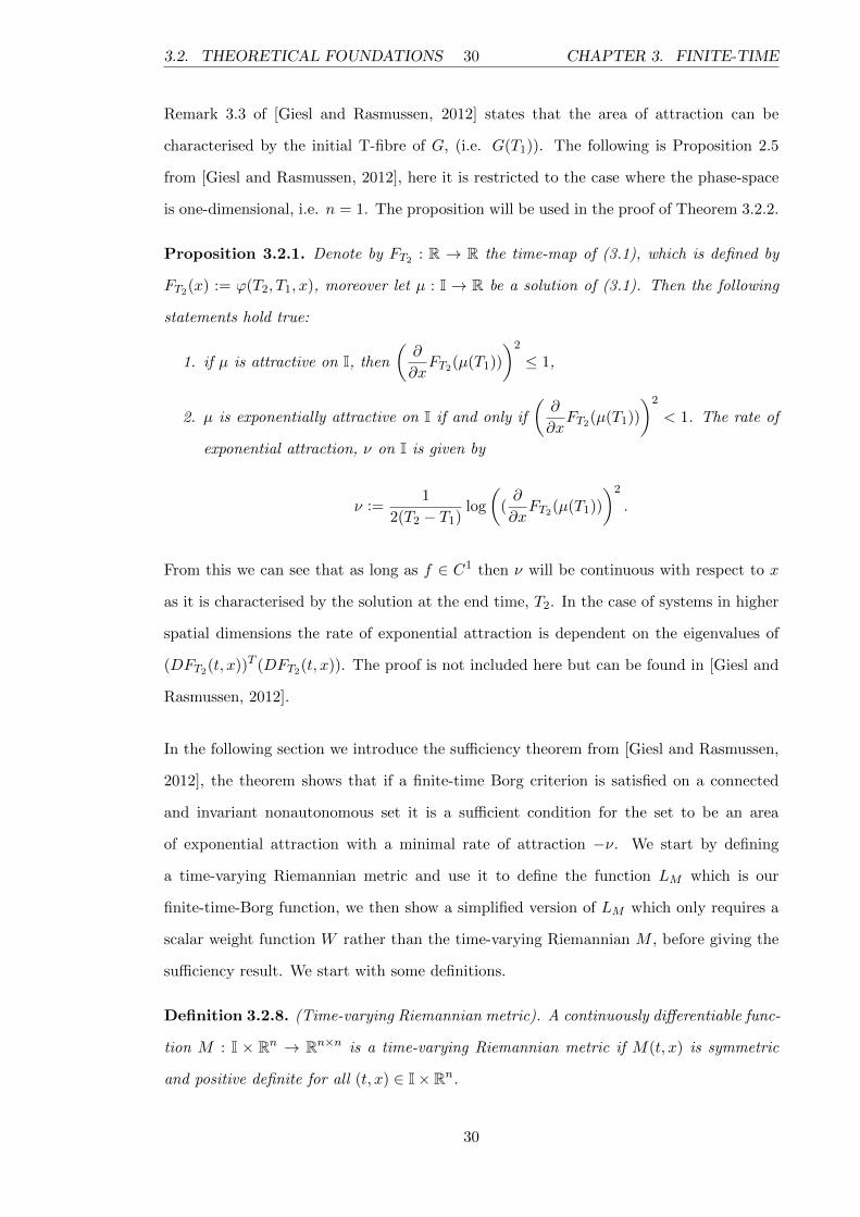
Remark 3.3 of [Giesl and Rasmussen, 2012] states that the area of attraction can be
characterised by the initial T-fibre of G, (i.e. G(T1)). The following is Proposition 2.5
from [Giesl and Rasmussen, 2012], here it is restricted to the case where the phase-space
is one-dimensional, i.e. n = 1. The proposition will be used in the proof of Theorem 3.2.2.
Proposition 3.2.1. Denote by FT2 : R → R the time-map of (3.1), which is defined by
FT2(x) := ϕ(T2, T1, x), moreover let µ : I → R be a solution of (3.1). Then the following
statements hold true:
1. if µ is attractive on I, then
(∂
∂xFT2(µ(T1))
)2
≤ 1,
2. µ is exponentially attractive on I if and only if
(∂
∂xFT2(µ(T1))
)2
< 1. The rate of
exponential attraction, ν on I is given by
ν :=1
2(T2 − T1)log
((∂
∂xFT2(µ(T1))
)2
.
From this we can see that as long as f ∈ C1 then ν will be continuous with respect to x
as it is characterised by the solution at the end time, T2. In the case of systems in higher
spatial dimensions the rate of exponential attraction is dependent on the eigenvalues of
(DFT2(t, x))T (DFT2(t, x)). The proof is not included here but can be found in [Giesl and
Rasmussen, 2012].
In the following section we introduce the sufficiency theorem from [Giesl and Rasmussen,
2012], the theorem shows that if a finite-time Borg criterion is satisfied on a connected
and invariant nonautonomous set it is a sufficient condition for the set to be an area
of exponential attraction with a minimal rate of attraction −ν. We start by defining
a time-varying Riemannian metric and use it to define the function LM which is our
finite-time-Borg function, we then show a simplified version of LM which only requires a
scalar weight function W rather than the time-varying Riemannian M , before giving the
sufficiency result. We start with some definitions.
Definition 3.2.8. (Time-varying Riemannian metric). A continuously differentiable func-
tion M : I × Rn → Rn×n is a time-varying Riemannian metric if M(t, x) is symmetric
and positive definite for all (t, x) ∈ I× Rn.
30

3.2. THEORETICAL FOUNDATIONS 31 CHAPTER 3. FINITE-TIME
As we are interested in the case of n = 1 our time-varying-Riemannian metric will be
positive scalar. In [Giesl and Rasmussen, 2012] the following definition is given for the
Borg-like function.
Definition 3.2.9. (LM ). Given a Riemannian metric M we define the following function
LM (t, x; v) := vT(M(t, x)Dxf(t, x) +
1
2M ′(t, x)
)v,
and
LM (t, x) := maxv∈Rn, vTM(t,x)v=1
LM (t, x; v).
Where M ′(t, x) := Mt + 〈∇M(t, x), f(t, x)〉.
By restricting the spatial dimension to one we can take the Riemannian metric to be of
the form e2W (t,x) where W ∈ C1(I × R,R), this is shown in the proceeding corollary. It
is a similar result to that given by Corollary 14 from [Giesl, 2004a] for the periodic orbit
case.
Corollary 3.2.1. If the restrictions that n = 1 and M(t, x) = e2W (t,x) are imposed with
W ∈ C1(I× R,R) then LM (t, x) satisfies the following
LM (t, x) = fx(t, x) +W ′(t, x).
Proof. Firstly note that with n = 1 the maximum condition in the definition of LM
becomes M(t, x) =1
v2with v ∈ R, so LM (t, x) = fx(t, x) +
M ′(t, x)
2M(t, x), then the result
follows.
Here we introduce the sufficiency condition (Theorem 4.2) from [Giesl and Rasmussen,
2012], as all connected intervals of R will be convex we can also absorb Corollary 4.3
from [Giesl and Rasmussen, 2012] into the theorem. We give a version that uses the result
of Corollary 3.2.1 to reduce the Riemannian metric to a scalar weight function.
Theorem 3.2.1. Consider the differential equation (3.1), let G ⊂ I × R be a nonempty,
connected, compact and invariant nonautonomous set and let W ∈ C1(G) with W (T1, x) =
0 for all x ∈ G(T1) and W (T2, x) = 0 for all x ∈ G(T2). Let M(t, x) = e2W (t,x) and assume
31

3.2. THEORETICAL FOUNDATIONS 32 CHAPTER 3. FINITE-TIME
that there exists a ν > 0 such that
LM (t, x) ≤ −ν, for all (t, x) ∈ G.
Then G is an area of exponential attraction. Furthermore
‖ϕ(T2, T1, x)− ϕ(T2, T1, y)‖ ≤ e−ν(T2−T1)‖x− y‖ for all x, y ∈ G(T1),
i.e. all solutions in G are exponentially attractive with a rate of at least ν.
Although this is not new work we include the proof as it is instructive in understanding
how the finite-time-Borg criterion relates to areas of exponential attraction. The proof
works by showing that if the finite-time-Borg function is bounded above by a negative
number then the distance, with respect to the weight-function, between the trajectories
within a δ-neighbourhood of any point in the t-fibre G(T1) will decrease at an exponential
rate of at least ν at time T2. Finally the result is expanded beyond the δ-neighbourhood
by using that the t-fibre G(T1) is connected and hence convex as it is in R.
Proof. We start by showing that for all γ < ν, there exists a δ > 0 such that for all
x0 ∈ G(T1), we have the following
‖ϕ(T2, T1, x0)− ϕ(T2, T1, η)‖ ≤ e−ν(T2−T1)‖x0 − η‖ for all η ∈ Bδ(x0). (3.2)
Let γ < ν, as fx (the derivative of f with respect to x) is continuous it is uniformly
continuous on G, hence there exists a δ1 > 0 such that
‖fx(t, x0)− fx(t, η)‖ ≤ ν − γ for all (t, x0) ∈ G and η ∈ Bδ1(x0).
Fix x0 ∈ G(T1) and η ∈ R with ‖η− x0‖ ≤ δ :=δ1
2and let µ(t) = ϕ(t, T1, x0) for all t ∈ I.
We define a time-varying distance by
Γ(t) := eW (t,µ(t))‖ϕ(t, T1, η)− µ(t)‖ for all t ∈ I. (3.3)
We note that Γ(T1) = ‖η − x0‖ giving that Γ(T1) ≤ δ1
2and hence there exists a maximal
θ > T1 such that Γ(t) ≤ δ1 for all t ∈ [T1, θ]. To show that γ decreases exponentially on
32

3.2. THEORETICAL FOUNDATIONS 33 CHAPTER 3. FINITE-TIME
[T1, θ] we take the temporal derivative of Γ2
d
dtΓ2(t) = 2W ′(t, µ(t))e2W (t,µ(t))‖ϕ(t, T1, η)− µ(t)‖2
+ 2e2W (t,µ(t))(ϕ(t, T1, η)− µ(t)
)(f(t, ϕ(t, T1, η))− f(t, µ(t))
),
= 2Γ2(t)W ′(t, µ(t)) + 2Γ2(t)
∫ 1
0fx(t, µ(t) + λ(ϕ(t, T1, η)− µ(t))
)dλ,
= 2Γ2(t)(W ′(t, µ(t)) + fx(t, µ(t))
)︸ ︷︷ ︸
=LM (t,µ(t))≤−ν
+ 2Γ2(t)
∫ 1
0
[fx(t, µ(t) + λ(ϕ(t, T1, η)− µ(t))
)− fx(t, µ(t))
]dλ,
≤ 2(ν − γ − ν)Γ2(t).
Hence
Γ(t) ≤ e−γ(t−T1)Γ(T1) for all t ∈ [T1, θ]. (3.4)
Therefore Γ(t) ≤ δ1
2for all t ∈ [T1, θ], if θ < T2 then the maximality of θ is contradicted,
hence it holds for all t ∈ [T1, T2]. As a result (3.2) holds true for any x0 ∈ G(T1).
To extend the proof over all x, y ∈ G(T1) we follow the methodology of Corollary 4.3
from [Giesl and Rasmussen, 2012]. Fix x and y as arbitrary values in G(T1). We note
that there exists a κ ∈ R+ with κ < δ and m ∈ N such that κm = ‖x − y‖. Therefore
y = x+κmy − x‖y − x‖
. Since G(T1) is connected and we are working in R it is convex, hence
we can take xi = x + κiy − x‖y − x‖
for i = 0, ..,m and will have that each xi ∈ G(T1) for
i = 0, ..,m. Then for each xi and xi+1 such that i < m we can make use of (3.4). Through
repeated use of the above argument we get the desired result that
‖ϕ(T1, T2, x)− ϕ(T1, T2, y)‖ ≤e−γ(T2−T1)‖x− y‖.
The next theorem is based upon the necessity results, Theorem 5.1, from [Giesl and Ras-
mussen, 2012]. However it is a modified version. Firstly we use the weight function version
of LM introduced in Corollary 3.2.1. Secondly it gives a partial differential equation con-
taining W , Theorem 5.1 in [Giesl and Rasmussen, 2012] only gives an inequality containing
33

3.2. THEORETICAL FOUNDATIONS 34 CHAPTER 3. FINITE-TIME
the finite-time Riemannian metric. This is a new result and will later allow for a collo-
cation equation to be formed that will be used to approximate W ′ and hence the area of
exponential attraction.
Theorem 3.2.2. Consider the differential equation (3.1) with n = 1 and f ∈ Cσ(I×R,R)
with σ ≥ 2 and a compact nonautonomous set G ⊂ I× R which is an area of exponential
attraction. Let −ν < 0 be the maximal rate of exponential attraction of all solutions
in G. Then there exists a continuous function W : G → R with W ∈ Cσ−1(G) and
W (T1, x) = W (T2, x) = 0 for x ∈ R such that
LM (t, x) = fx(t, x) +W ′(t, x) ≤ −ν for all (t, x) ∈ G,
and
fx(t, ϕ(t, T1, x)) +W ′(t, ϕ(t, T1, x)) = γ(x) for all (t, x) ∈ I×G(T1). (3.5)
Where γ(x) is the exponential rate of attraction of the solution ϕ(t, T1, x)) on I with initial
condition x.
Proof. We start by considering a fixed initial value and its associated solution, we begin
to construct a Riemannian metric M for that solution in similar fashion as Theorem 5.1
in [Giesl and Rasmussen, 2012]. Fix a x0 ∈ G(T1) and let µ be the associated solution
with µ(t) = ϕ(t, T1, x0). Consider the variational form associated with this solution
y = fx(t, µ(t))y. (3.6)
We follow an approach based on Floquet theory, denote the (fundamental) solution of
(3.6) as φ : I → R, then the solution will take the form φ(t) = e∫ tT1fx(τ,µ(τ))dτ
. We
build the metric in a similar way to how P (t) from Floquet theory is built (Section 2.4
[Chicone, 2000]) and use the fact that the solution of the variational form satisfies φ(t) =
∂
∂xFt(µ(T1)), where Ft is the time map defined in Proposition 3.2.1. We combine this
along with Proposition 3.2.1 to give
γ(x0) =1
2(T2 − T1)log(φ2(T2)).
34

3.3. AN APPROXIMANT FOR W 35 CHAPTER 3. FINITE-TIME
or conversely that
φ(T2) = eγ(x0)(T2−T1).
Where γ(x0) is the rate of exponential attraction for the solution µ (from Proposition
3.2.1). It should be noted that due to its characterisation in Proposition 3.2.1 γ(x) will be
Cσ−1 in space and its orbital derivative satisfies γ′(x) = 0. The metric can be constructed
as
M(t, µ(t)) := φ−2(t)e2γ(x0)(t−T1). (3.7)
We now define W as
W (t, x) :=1
2log(M(t, x)). (3.8)
Therefore by combining (3.7) and (3.8) we get
W (t, µ(t)) = − log(φ(t)) + γ(x0)(t− T1),
= −∫ t
T1
fx(τ, µ(τ))dτ + γ(x0)(t− T1). (3.9)
from this it is clear that W ∈ Cσ−1. We can take the orbital derivative to give
W ′(t, µ(t)) = −fx(t, µ(t)) + γ(x0).
Since M(T1, µ(T1)) = M(T2, µ(T2)) = 1 then recalling from (3.8) that M(t, x) = e2W (t,x)
we see that W (T1, µ(T1)) = W (T2, µ(T2)) = 0. Finally by virtue of G being an area of
exponential attraction with maximal rate −ν and LM (t, x) we have the other result.
3.3 An Approximant for W
Theorem 3.2.2 gives an equation involving W ′, however it cannot yet be used to construct
an approximation to W ′ as γ is unknown. We seek to form a collocation equation that
only involves a linear differential operation applied to W and known values on the right
hand side. Proposition 3.2.1 shows γ is constant along solutions, this allows us to take
the orbital derivative of (3.5) to derive a linear partial differential equation where W is
35

3.3. AN APPROXIMANT FOR W 36 CHAPTER 3. FINITE-TIME
the only unknown. We also confirm that LM is constant along solutions. These are both
shown in the following corollary.
Corollary 3.3.1. Let the conditions of Theorem 3.2.2 be satisfied, then the following two
statements are true
W ′′(t, x) = −fx(t, x)′
= −(fxt(t, x) + fxx(t, x)f(t, x)) for all (t, x) ∈ G, (3.10)
and
L′M (t, x) = 0 for all (t, x) ∈ G. (3.11)
Proof. The proof of both statements is very simple, firstly we prove (3.10). From Theorem
3.2.2 we have that
fx(t, ϕ(t, T1, x)) +W ′(t, ϕ(t, T1, x)) = γ(x) for all (t, x) ∈ I×G(T1).
Then by taking the orbital derivative and noting that Proposition 3.2.1 gives that γ is
constant along solutions we get (3.10). For the second statement we note that by Corollary
3.2.1 we have for all (t, x) ∈ I×G(T1),
LM (t, x) = fx(t, x) +W ′(t, x).
Then by taking the orbital derivative of the above equation we get,
L′M (t, x) = (W ′(t, x) + fx(t, x))′,
= W ′′(t, x) + (fxt(t, x) + fxx(t, x)f(t, x)).
Then by using (3.10) we immediately see (3.11) is true.
Corollary 3.3.1 gives a partial differential equation which can be numerically solved to
give W . We can then use W to construct an approximation of the area of exponential
attraction. To approximate a subset of the area of attraction with a given maximal rate
of exponential attraction λ, we wish to find a level set of LM = λ which is equal to that
36

3.3. AN APPROXIMANT FOR W 37 CHAPTER 3. FINITE-TIME
value. To clarify that this is an area of exponential attraction we bring together the results
of Theorem 3.2.1 and Theorem 3.2.2 to explicitly state that the set bounded by the level
sets where the rate of exponential attraction, λ, is an area of exponential attraction. The
following corollary confirms that the function W that satisfies W ′′ = −f ′x on the interior
of the domain and W = 0 on the boundary is the same function W from Theorem 3.2.2
and that it characterises an area of exponential attraction.
Corollary 3.3.2. Consider the differential equation (3.1) with n = 1 and f ∈ Cσ(I×R,R)
with σ ≥ 2 and a compact nonautonomous set G ⊂ I× R which is an area of exponential
attraction. Let −ν < 0 be the maximal rate of exponential attraction of all solutions in
G. Then there exists a function W ∈ Cσ−1(G,R) which satisfies W ′′(t, x) = −(fx(t, x))′.
Conversely consider a nonempty, connected, compact and invariant nonautonomous set
G1 ⊂ I× R, assume the function W ∈ Cσ−1(G1,R) solves the boundary value problem
• W (t, x) = 0 for all (t, x) ∈ G1(T1),
• W (t, x) = 0 for all (t, x) ∈ G1(T2),
• W ′′(t, x) = −(fx(t, x))′ for all (t, x) ∈ G1.
Then W is the function described in Theorem 3.2.2 and LM (t, µ(t)) is constant for all t ∈ I.
Furthermore there exist x1, x2 ∈ G1(T1) with x1 < x2, ϕ(t, T1, x1) ∈ G1, ϕ(t, T1, x2) ∈ G1
satisfying the following conditions and λ < 0,
• LM (T1, x1) = λ,
• LM (T1, x2) = λ,
• LM (T1, x) ≤ λ, for all x ∈ (x1, x2).
Then the set enclosed by (T1, x1) to (T1, x2), (T2, ϕ(T2, T1, x1)) to (T2, ϕ(T2, T1, x2)) and
the lines (t, ϕ(t, T1, x1)) | t ∈ I and (t, ϕ(t, T1, x2)) | t ∈ I will be an area of exponential
attraction on I with maximal rate of exponential attraction λ.
Proof. We fix x0 ∈ G1(T1) and take µ(t) = ϕ(t, T1, x0). By integrating W ′′(t, x) along
37

3.3. AN APPROXIMANT FOR W 38 CHAPTER 3. FINITE-TIME
µ(t) we obtain the following
∫ t
T1
W ′′(τ, µ(τ))dτ = −∫ t
T1
(fx(τ, µ(τ))
)′dτ,
(⇔) W ′(t, µ(t)) = −fx(τ, µ(τ)) + c. (3.12)
We integrate (3.12) again between the temporal boundaries
0 =
∫ T2
T1
W ′(τ, µ(τ))dτ = −∫ T2
T1
fx(τ, µ(τ))dτ + c(T2 − T1).
This gives,
c =
∫ T2
T1fx(τ, µ(τ))dτ
T2 − T1. (3.13)
From (3.9) we have 0 = W (T2, µ(T2)) = −∫ T2
T1
fx(τ, µ(τ))dτ+γ(x0)(T2−T1). Rearranging
this and (3.13) gives us that c = γ(x0). Therefore the function W given in this corollary
satisfies W ′(t, µ(t)) = −fx(t, µ(t)) + γ(x0). It is therefore the same function as given in
Theorem 3.2.2. Furthermore, as LM (t, µ(t)) = γ(x0) and γ(x0) is constant along solutions
by definition cf. Proposition 3.2.1 we have that L′M (t, µ(t)) = 0. The second part of the
corollary immediately follows from Theorem 3.2.2 where it is shown that γ(x0) is the rate
of exponential attraction for the solution ϕ(t, T1, x0).
3.3.1 Meshfree Collocation
In order to construct the approximation to W and hence LM we will use meshfree collo-
cation with compactly supported radial basis functions. We will be using the symmetric
method of generalised interpolation that is described in Chapter 2 to approximate the
boundary value problem that is described below.
Let us define the region of interest as G ⊂ I × R and let the temporal boundary of G be
called Γ := G(T1) ∪G(T2). The boundary value problem can be described as
W ′′(t, x) = −(fx(t, x))′ for (t, x) ∈ G, (3.14)
W (t, x) = 0 for all (t, x) ∈ Γ.
38

3.3. AN APPROXIMANT FOR W 39 CHAPTER 3. FINITE-TIME
Let us define our collocation points, the set of interior points X := xi = (ti, xi) ∈ G
for i = 1, ..., N and data points on the temporal boundary XΓ := ηj = (τj , ηj) ∈ Γ for
j = 1, ..., N1. The ansatz for the approximation will be
w(t, x) =N∑k=1
αk (δxk L)y Ψ(x− y) +
N1∑k=1
βk (δηk)y Ψ(x− y). (3.15)
Where the differential operator Lw(t, x) = w′′(t, x) and the coefficient vector (α, β)T ∈
RN+N1 is determined by the following collocation system
(δxj L)(w) = (δxj L)(W ) = −f ′x(xj),
(δηj )(w) = (δηj )(W ) = 0.
The linear system becomes
A C
CT B
α
β
=
a
b
,
where A ∈ RN×Nwith entries Aik = (δxi L)x(δxk L)yΨ(x− y),
where C ∈ RN×N1with entries Cik = (δxi L)x(δηk)yΨ(x− y),
where B ∈ RN1×N1with entries Bik = (δηk)x(δηk)yΨ(x− y),
where a ∈ RN with entries ai = −f ′x(xi),
where b ∈ RN1 with entries bi = 0,
and (α, β)T is a RN+N1 coefficient vector to be determined.
As the radial basis function is a positive definite function and we have used symmetric
collocation this system has a solution. The following shows the results of the pointwise
and differential operators being applied to a general radial basis function. We remind the
reader of the recursive notation introduced in Chapter 2 to define the different differential
powers of ψ, ψi =1
r
∂ψi−1(r)
∂r. The first is the boundary point operator, (δηi), being applied
to interior points of the ansatz, (3.15). This and the following results come from [Giesl,
39
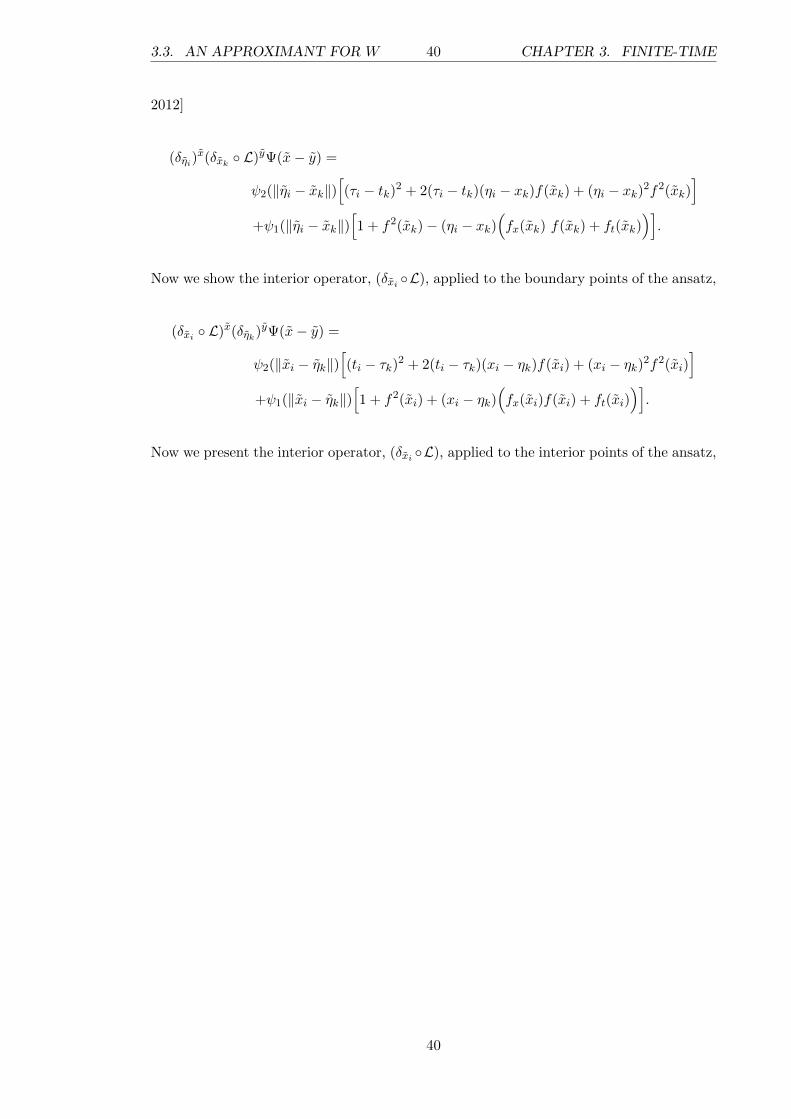
3.3. AN APPROXIMANT FOR W 40 CHAPTER 3. FINITE-TIME
2012]
(δηi)x(δxk L)yΨ(x− y) =
ψ2(‖ηi − xk‖)[(τi − tk)2 + 2(τi − tk)(ηi − xk)f(xk) + (ηi − xk)2f2(xk)
]+ψ1(‖ηi − xk‖)
[1 + f2(xk)− (ηi − xk)
(fx(xk) f(xk) + ft(xk)
)].
Now we show the interior operator, (δxi L), applied to the boundary points of the ansatz,
(δxi L)x(δηk)yΨ(x− y) =
ψ2(‖xi − ηk‖)[(ti − τk)2 + 2(ti − τk)(xi − ηk)f(xi) + (xi − ηk)2f2(xi)
]+ψ1(‖xi − ηk‖)
[1 + f2(xi) + (xi − ηk)
(fx(xi)f(xi) + ft(xi)
)].
Now we present the interior operator, (δxi L), applied to the interior points of the ansatz,
40

3.3. AN APPROXIMANT FOR W 41 CHAPTER 3. FINITE-TIME
(δxi L)x(δxk L)yΨ(x− y) =
ψ4
(‖xi − xk‖
)((ti − tk)2
((ti − tk) + (xi − xk)(f(xk) + f(xi))
)2
+(
(xi − xk)2f(xk)f(xi) + (ti − tk)(xi − xk)(f(xk) + f(xi)))2
− (ti − tk)2
[(xi − xk)f(xk)]2 + [(xi − xk)f(xi)]
2)
+ψ3
(‖xi − xk‖
)((ti − tk)
[(ti − tk) + (xi − xk)(f(xk) + f(xi))
][6 + 4f(xk)f(xi)
]+ f2(xi)
(xi − xk)f(xk) + (ti − tk))
2
+ f2(xk)
(xi − xk)f(xi) + (ti − tk))2
+ [(xi − xk)2(f2(xk) + f2(xi)
)+ 4(xi − xk)2f(xk)f(xi)][1 + f(xk)f(xi)]
+
(ti − tk) + (xi − xk)f(xk)2[(xi − xk)
(fx(xi)f(xi) + ft(xi)
)]−
(ti − tk) + (xi − xk)f(xi)2[(xi − xk)
(fx(xk)f(xk) + ft(xk)
)]+ψ2
(‖xi − xk‖
)(3 + f2(xk) + f2(xi)
+ 4[f(xk)f(xi)] + 3[f(xk)f(xi)]2
−(1 + f2(xi)
)[(xi − xk)
(fx(xk)f(xk) + ft(xk)
)]+(1 + f2(xk)
)[(xi − xk)
(fx(xi)f(xi) + ft(xi)
)]− (xi − xk)2
(fx(xk)f(xk) + ft(xk)
)(fx(xi)f(xi) + ft(xi)
)+ 2[(ti − tk) + (xi − xk)f(xk)
][f(xk)
(fx(xi)f(xi) + ft(xi)
)]− 2[(ti − tk) + (xi − xk)f(xi)
][f(xi)
(fx(xk)f(xk) + ft(xk)
)])−ψ1
(‖xi − xk‖
)(fx(xk)f(xk) + ft(xk)
)(fx(xi)f(xi) + ft(xi)
).
Finally to approximate the area of exponential attraction we need to know the orbital
derivative of the anstaz w(x). To approximate this we introduce a new differential operator
D, it will be the orbital derivative so Dw(x) = w′(x) = vt(x) + vx(x) · f(x), with x ∈ I×R
w′(x) =
N∑k=1
αk (δx D)x (δxk L)y Ψ(x− y) +
N1∑k=1
βk (δx D)x (δηk)y Ψ(x− y),
41

3.3. AN APPROXIMANT FOR W 42 CHAPTER 3. FINITE-TIME
which becomes,
w′(x) =
N∑k=1
αk
[ψ3(‖x− xk‖)
((t− tk)3 + 2(t− tk)2(x− xk)f(xk) + (t− tk)[(x− xk)f(xk)]
2
+ (x− xk)f(x)(
(t− tk)2 + 2(t− tk)(x− xk)f(xk))
+ (x− xk)f(x)[(x− xk)f(xk)]2
)+ψ2(‖x− xk‖)
(3(t− tk) + 2(x− xk)f(xk) + (t− tk)f2(xk)
− (t− tk)(x− xk)[fx(xk)f(xk) + ft(xk)
]+ (x− xk)f(x)
(1 + f2(xk)− (x− xk)
[fx(xk)f(xk) + ft(xk)
])+ 2f(xk)f(x)
((t− tk) + (x− xk)f(xk)
))−ψ1(‖x− xk‖)
(f(x)
[fx(xk)f(xk) + ft(xk)
])]+
N1∑k=1
βkψ1(‖x− ηk‖)(
(t− τk) + (x− ηk)f(x)).
The linear system can be solved to determine the coefficient vector (α, β)T , then the
coefficient vector can be used to construct w′(x). Then by using the approximation of
w′(x) to determine level sets of Lm(x) one can approximate areas of exponential attraction.
3.3.2 Error Analysis
To show that the method is convergent we firstly make use of existing results on the
standard error estimates for radial basis functions in approximating generalised linear
differential equations found in [Giesl and Wendland, 2007] and presented in Chapter 2.
We use Corollary 3.11 from [Giesl and Wendland, 2007] to give a modified version of the
convergence proof, this version allows for the case where parts of the boundary, Γ, are not
connected. The main measure for node distance we use is the fill distance,
hG := supx∈G
infxj∈X
‖x− xj‖2,
we also need the fill distance along the temporal boundary
hΓ := supx∈Γ
infxj∈XΓ
‖x− xj‖2.
42

3.3. AN APPROXIMANT FOR W 43 CHAPTER 3. FINITE-TIME
The following theorem from [Giesl and Wendland, 2007] with the boundary condition
replaced with the one from Corollary 3.11 in [Giesl and Wendland, 2007] gives a general
convergence result with respect to the fill distances, for the interior of the domain and on
the temporal boundary.
Theorem 3.3.1. Fix τ ∈ R+ such that k := bτc > 4, σ := dτe and s := τ − k. Suppose
Ψ generates a reproducing kernel Hilbert space that is norm equivalent to W τ2 (I×R). Let
Ω ∈ I × R be a bounded domain having a piecewise Ck,s-boundary. Finally, let w be the
approximant to W ∈W τ2 (Ω) satisfying (3.14).
If the data have sufficiently small mesh-norms, then for all 1 ≤ p ≤ ∞ the error estimates
‖LW − Lw‖Lp(Ω) ≤ Chτ−2−2(1/2−1/p)+
G ‖W‖W τ2 (G),
‖W − w‖Lp(Γ) ≤ Chτ−1/2−(1/2−1/p)+
Γ ‖W‖W τ2 (Ω),
are satisfied.
The proof for this theorem is given in [Giesl and Wendland, 2007]. We show here that its
application is appropriate for our situation. Indeed, the differential operator LW = W ′′
is of order 2 with coefficients cα ∈W k−1∞ (Ω).
The above theorem can be applied to our approximation to give error bounds on the
interior between w′′ and W ′′, and bounds between w and W on the boundary. The
convergence result from the previous theorem can then be used to give an error bound for
LM and our approximation Lm, to do this we make use of a lemma from [Giesl, 2012].
Lemma 3.3.1. Let q, Q ∈ C2(I) be functions with, q(T1) = a, q(T2) = b, |q′′(t)| ≤ ε for
all t ∈ (T1, T2), Q(T1) = A, Q(T2) = B, Q′′(t) = 0 for all t ∈ (T1, T2). Then we have for
all t ∈ [T1, T2]
|Q′(t)− q′(t)| ≤ |A− a|+ |B − b|T2 − T1
+3
2(T2 − T1)ε, (3.16)
|Q(t)− q(t)| ≤ 2|A− a|+ |B − b|+ (T2 − T1)2ε, (3.17)
Q′(t) =B −AT2 − T1
. (3.18)
The proof comes from simple calculus, and comes from an earlier version of [Giesl, 2012].
43
3.3. AN APPROXIMANT FOR W 44 CHAPTER 3. FINITE-TIME
Proof. By integration we obtain
q′(t) =
∫ t
T1
q′′(τ)dτ + c, (3.19)
q(t) =
∫ t
T1
∫ θ
T1
q′′(τ)dτdθ + c(t− T1) + a, (3.20)
where the second integration constant was chosen such that q(T1) = a. As q(T2) = b, from
(3.20) we have
b = q(T2),
=
∫ T2
T1
∫ θ
T1
q′′(τ)dτdθ + c(T2 − T1) + a, i.e.
c =b− a−
∫ T2
T1
∫ θT1q′′(τ)dτdθ
T2 − T1. (3.21)
Note that
∫ T2
T1
∫ θ
T1
q′′(τ)dτdθ =
∫∆q′′(τ)dτdθ, where ∆ denotes the triangle ∆ = (θ, τ) ∈
R2 | T1 < θ < T2, T1 < τ < θ of area1
2(T2 − T1)2. Thus
∣∣∣∣∫∆q′′(τ)dτdθ
∣∣∣∣ ≤ 1
2(T2 − T1)2ε.
We also integrate the function Q, taking the boundary conditions into account. We obtain
Q′(t) =B −AT2 − T1
,
Q(t) =B −AT2 − T1
(t− T1) +A.
This shows (3.18). Thus, we can calculate the following, using (3.19), (3.20) and (3.21),
|Q′(t)− q′(t)| ≤(T2 − T1)ε+|B −A− (b− a)|
T2 − T1+
1
2(T2 − T1)ε,
≤|A− a|+ |B − b|T2 − T1
+3
2(T2 − T1)ε.
|Q(t)− q(t)| ≤1
2(T2 − T1)2ε+
∣∣∣∣ B −AT2 − T1− c∣∣∣∣ (T2 − T1) + |A− a|,
≤(T2 − T1)2ε+|B − b|+ |A− a|
T2 − T1(T2 − T1) + |A− a|,
=2|A− a|+ |B − b|+ (T2 − T1)2ε.
44

3.3. AN APPROXIMANT FOR W 45 CHAPTER 3. FINITE-TIME
Thus proving the lemma.
Using the Lemma 3.3.1 we now bound the error between our approximation and the true
LM .
Theorem 3.3.2. Let µ(t) be an solution to (3.1) with rate of attraction γµ. Let Lm be
the approximation to LM constructed by the method laid out in this section, and let the
mesh norms be such that ‖W ′′(t, x)−w′′(t, x)‖L∞(G) ≤ ε for all (t, x) ∈ G and ‖W (t, x)−
w(t, x)‖L∞(Γ) ≤ δ for all (t, x) ∈ Γ and f ∈ Ck(I,R) with k ≥ 3 then
|Lm(t, µ(t))− γµ| ≤δ
T2 − T1+
3(T2 − T1)ε
4for all t ∈ I.
Proof. Let Q(t) := W (µ(t)) +
∫ t
T1
fx(τ, µ(τ))dτ , q(t) := w(µ(t)) +
∫ t
T1
fx(τ, µ(τ))dτ , since
f ∈ Ck we have from Theorem 3.2.2 that W ∈ Ck−1. Then Q and q are functions that
satisfy the properties of Lemma 3.3.1 with,
q(T1) = w(T1, µ(T1)) +
∫ T1
T1
fx(τ, µ(τ))dτ = a,
q(T2) = w(T2, µ(T2)) +
∫ T2
T1
fx(τ, µ(τ))dτ = b,
q′′(t) = w′′(t, µ(t)) + f ′x(t, µ(t)).
Q(T1) = W (T1, µ(T1)) +
∫ T1
T1
fx(τ, µ(τ))dτ = A,
Q(T2) = W (T, µ(T2))) +
∫ T2
T1
fx(τ, µ(τ))dτ = B,
Q′′(t) = W ′′(t, µ(t)) + f ′x(t, µ(t)) = 0.
As W ′′(t, µ(t)) = −f ′x(t, µ(t)) we have that
|q′′(t)| = |w′′(t, µ(t))−W ′′(t, µ(t))| ≤ ε
.
Also as |A−a| = |w(T1, µ(T1))−W (T1, µ(T1))| ≤ δ as it is on the temporal boundary, the
same holds for |B − b| ≤ δ. Then as LM (t, µ(t)) = W ′(t, µ(t)) + fx(t, µ(t)) = γµ we can
45

3.4. EXAMPLES 46 CHAPTER 3. FINITE-TIME
use this along with Lemma 3.3.1 to give,
|Lm(t, µ(t))− γµ| = |LM (t, µ(t))− Lm(t, µ(t))|,
= |W ′(t, µ(t))− w′(t, µ(t))|,
= |Q′(t)− q′(t)|,
≤ 2δ
T2 − T1+
3(T2 − T1)
2ε.
giving the desired result.
Remark
From Theorem 3.3.2 we have that |Lm(t, µ(t)))−γµ| ≤ ε∗. Therefore the approximation of
the area of exponential attraction with maximal rate of attraction −ν will be given by the
set Gε∗ := (t, x)|Lm(t, x) = −ν − ε∗. This will not necessarily be an area of exponential
attraction as there is no guarantee that Gε∗ will be invariant. However we can say that
Gε∗ ⊂ G−ν where G−ν := (t, x)|LM (t, x) ≤ −ν. This can be seen from the fact that
(t, x)|LM (t, x) = −ν ⊂ (t, x)| − ν − ε∗ ≤ Lm(t, x) ≤ −ν + ε∗.
3.4 Examples
3.4.1 Analytically Solvable System
We will consider the following example with x ∈ R
x = x(x− 1), I = [0, 1]. (3.22)
We use the Radial Basis Function ψ6,4(2r) as seen in Table 2.2 to construct our approx-
imation w of W , the solution of the boundary problem given in Corollary 3.3.2. On the
boundary we use the following points X2 := (t, x) | t ∈ 0, 1, x ∈ 0, 0.05, 0.1, . . . , 0.8.
For the interior points we take X1 := (t, x) | t ∈ 0.025, 0.075, 0.125, . . . , 0.975, x ∈
0, 0.05, 0.1, . . . , 0.8. We show X1 and X2 as well as some numerically approximated
solutions in Figure 3.1.
It is shown in [Giesl and Rasmussen, 2012] that the rate of exponential attraction for the
46

3.4. EXAMPLES 47 CHAPTER 3. FINITE-TIME
0 0.1 0.2 0.3 0.4 0.5 0.6 0.7 0.8 0.9 10
0.1
0.2
0.3
0.4
0.5
0.6
0.7
0.8
t
x
Figure 3.1: The sets of the interior points, X1 and boundary points X2
used in the construction of w are shown. Also shown are some solutionsof the system given in (3.22).
solution ϕ(t, 0, x0) is given by
γ(x0) := 1− 2
T2ln(x0 − (x0 − 1)eT2) for all x0 ∈
(−∞, e1
e1 − 1
).
where T2 = 1. We use this form of γ and an inverse map of the solution to derive LM (t, x).
This allows us to compare the approximation Lm(t, x) directly with the function it is
approximating. A plot of Lm(t, x) is given in Figure 3.2.
In Figure 3.3 we produce a plot of the level sets of Lm(t, x). In our approximation we have
Lm(0, 0.6229) ≈ 0. We define ε0 :=2δ
T2 − T1+
3(T2 − T1)
2where ε and δ are from Theorem
3.3.2. Then we determine that a subset of the area of exponential attraction is given by
(t, x) | t ∈ I and x ∈ x | Lm(t, x) ≤ −ε0). The true boundary of the area of exponential
attraction is given by (t, x) | t ∈ I and x ≤ ϕ(t, 0, 0.γ0) where γ0 =e− e1/2
e− 1≈ 0.622459.
In Table 3.2 we show the error for different fill distances, the error was approximated on
a grid with h = 1/128 and was defined as max(t,x)∈Y1/128
‖W ′(t, x)− w′(t, x)‖, where Y1/128 is
the same as X1 ∪X2 except with a smaller fill distance. We took Ψ6,4 as our Wendland
function, [0, 1] as our time domain and and [0, 0.8] as the space domain, the points were
47

3.4. EXAMPLES 48 CHAPTER 3. FINITE-TIME
0
0.2
0.4
0.6
0.8
1
0
0.2
0.4
0.6
0.8−1.2
−1
−0.8
−0.6
−0.4
−0.2
0
0.2
0.4
0.6
tx
Figure 3.2: The approximation Lm(t, x) = w′(t, x) + fx(t, x).
uniformly placed in [0, 1]× [0, 0.8] and the support radius was1
2. There is some evidence
to support a convergence rate of 2 however as Theorem 3.3.2 does not give a theoretical
convergence rate in terms of the fill distance we cannot compare the numerical result.
−0.8
−0.8−0.8
−0.4
−0.4
−0.4
0
0
0
0
0.4
0.4
0.4
t
x
0 0.1 0.2 0.3 0.4 0.5 0.6 0.7 0.8 0.9 10
0.1
0.2
0.3
0.4
0.5
0.6
0.7
0.8
Figure 3.3: Level sets of Lm(t, x) = L, where L = −0.8,−0.4, 0, 0.4.
48

3.4. EXAMPLES 49 CHAPTER 3. FINITE-TIME
Table 3.1: Left: we give the max(t,x)∈Y1/128
‖W ′(t, x) − w′(t, x)‖, the error was computed on
a shifted mesh with h = 1/128. Right: We have numerically approximated convergencerates.
Table 3.2
h ‖W ′(t, x)− w′(t, x)‖∞1/8 0.21941/16 0.08931/32 0.01581/64 0.0080
Table 3.3
ε1/16/ε1/8 2.4579
ε1/32/ε1/16 5.6493
ε1/64/ε1/32 1.9789
3.4.2 Nonautonomous Example
For the second example we choose a nonautonomous Bernoulli type problem with x ∈ R
on the time interval [0, 2]. It was used to approximate the domain of attraction in [Giesl,
2012]. It is particularly nice example as the distance between trajectories both increases
and decreases along the time domain. The system is
x = x
(1
4− (t− 1)2 + x3
), I = [0, 2]. (3.23)
The solution is of the form,
ϕ(t, 0, x0)
= x0 exp
(−1
3t3 + t2 − 3
4
)(1− 2x2
0
∫ t
0exp
(−2
3τ3 + 2τ2 − 3
2τ
)dτ
)−1/2
.
Since
∫ t
0exp
(−2
3τ3 + 2τ2 − 3
2τ
)cannot be analytically solved we cannot determine an
analytic form of LM . We have used the Radial Basis Function ψ6,4(0.5r) as seen in Table
2.2 to construct our approximation w of the solution to the boundary problem given in
Corollary 3.3.2. For the boundary we use the following points X2 := (t, x) | t ∈ 0, 2, x ∈
−0.32,−0.28, . . . , 0, 0.04, . . . , 0.32. For the interior points we take X1 := (t, x) | t ∈
0.05, 0.15, 0.25, . . . , 1.95, x ∈ −0.32,−0.28, . . . , 0, 0.04, . . . , 0.32. We show X1 and X2
as well as some numerically approximated solutions in Figure 3.4.
Figure 3.6 show some level sets of Lm(x). We define ε0 :=2δ
T2 − T1+
3(T2 − T1)
2where ε
and δ are from Theorem 3.3.2. Then we determine that a subset of the area of exponential
attraction is given by (t, x) | t ∈ I and x ∈ x | Lm(t, x) ≤ −ε0). In this case we
determine that the level set of L(t, x) = 0 is given by x(0) ≈ ±0.1789. In Figure 3.7 we
49

3.4. EXAMPLES 50 CHAPTER 3. FINITE-TIME
0 0.2 0.4 0.6 0.8 1 1.2 1.4 1.6 1.8 2−0.4
−0.3
−0.2
−0.1
0
0.1
0.2
0.3
0.4
t
x
Figure 3.4: The sets of the interior points, X1 and boundary pointsX2 used in the construction of w are shown. Also shown are the somesolutions of the system given in (3.23).
0
0.5
1
1.5
2
−0.4
−0.2
0
0.2
0.4−0.1
0
0.1
0.2
0.3
0.4
0.5
0.6
tx
Figure 3.5: The approximation of Lm(t, x)
see that along this solution we closely mirror the zero-level set of Lm. Interestingly the
area of exponential attraction is well contained by the domain of attraction as shown in
50
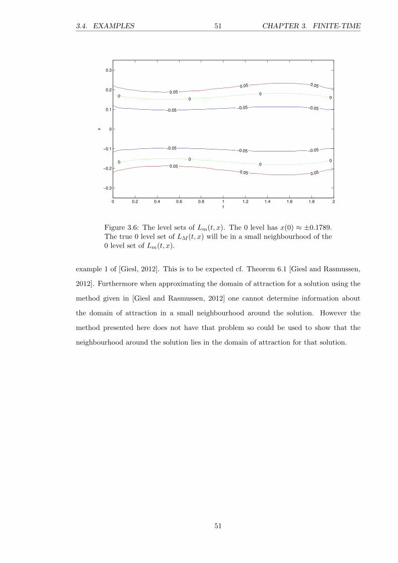
3.4. EXAMPLES 51 CHAPTER 3. FINITE-TIME
−0.05−0.05 −0.05
−0.05 −0.05 −0.05
00
00
00
00
0.05
0.05 0.05
0.05
0.05 0.05
t
x
0 0.2 0.4 0.6 0.8 1 1.2 1.4 1.6 1.8 2
−0.3
−0.2
−0.1
0
0.1
0.2
0.3
Figure 3.6: The level sets of Lm(t, x). The 0 level has x(0) ≈ ±0.1789.The true 0 level set of LM (t, x) will be in a small neighbourhood of the0 level set of Lm(t, x).
example 1 of [Giesl, 2012]. This is to be expected cf. Theorem 6.1 [Giesl and Rasmussen,
2012]. Furthermore when approximating the domain of attraction for a solution using the
method given in [Giesl and Rasmussen, 2012] one cannot determine information about
the domain of attraction in a small neighbourhood around the solution. However the
method presented here does not have that problem so could be used to show that the
neighbourhood around the solution lies in the domain of attraction for that solution.
51

3.4. EXAMPLES 52 CHAPTER 3. FINITE-TIME
0 0.2 0.4 0.6 0.8 1 1.2 1.4 1.6 1.8 20
0.5
1
1.5
2
2.5
3
3.5
4
4.5
5x 10
−3
t
Lm
(t,µ
(t))
Figure 3.7: We show Lm(t, µ(t)) where µ(t) = ϕ(t, 0, 0.1789).We numerically approximate µ(t) using Matlab’s ODE45 function.Lm(0, 0.1789) = 0 to four significant figures.
52

53 CHAPTER 4. PERIODIC ORBITS
Chapter 4
Approximating the basin of
attraction of a periodic orbit in
two dimensions
4.1 Introduction
This chapter shows a new method for approximating the basin of attraction of an expo-
nentially stable periodic orbit in R2. The method also gives the existence and uniqueness
of that periodic orbit within a compact and positively invariant set. It extends the exist-
ing work [Giesl, 2007b], in which a method for determining the basin of attraction of an
exponentially stable periodic orbit is given; that method also establishes both the unique-
ness and existence of the orbit within a compact invariant set. The difference between
the two methods is that in [Giesl, 2007b] the method requires attributes of the periodic
orbit to be numerically approximated. Both methods have an advantage over the more
traditional Lyapunov methods for determining basins of attraction, which require exact
knowledge of where the periodic orbit is. The work in this chapter adds to the field a
method for determining a subset of the basin of attraction of periodic orbit that does not
require knowledge of any of the attributes of the orbit.
The work in this chapter is presented in two main parts. The first contains the theoretical
foundation for the following sections. It shows that if a special contraction function is
negative on a compact, positively invariant set that does not contain an equilibrium point,
53

4.2. THEORETICAL FOUNDATIONS 54 CHAPTER 4. PERIODIC ORBITS
it is both a necessary and sufficient condition for that set to be a subset of the basin of
attraction of a unique exponentially stable periodic orbit. In the theorem that gives the
necessity condition we derive an equation that will go on to be used to approximate the
contraction function. This is not new work, it is based upon results in [Giesl, 2007b], [Giesl,
2004a] and [Giesl, 2003]; but it is an important foundation for why the methodology works.
Where possible the author has paraphrased the work and simplified the mathematical
methodologies, as the scope of this chapter is restricted to two dimensions.
Section 4.3 describes the new methodology that approximates the basin of attraction for
the exponentially stable periodic orbit. This new methodology is a significant advancement
in the field since, as far as the author is aware, it is the first method to approximate a
subset of the basin of attraction that needs neither explicit knowledge of the location of the
periodic orbit nor other attributes of the periodic orbit to be approximated. This allows
it to be applied to systems where explicit knowledge of the orbit is not known. Section 4.3
also shows how the method is derived from the theoretical foundations covered in Section
4.2. In Section 4.4 we show that the error in the approximation of W ′ will decrease as
denser meshes are used. Finally in Section 4.5 two examples are given: the first is a toy
problem that can solved analytically, and the second is a problem that can only be solved
numerically and has been used previously in the existing literature.
4.2 Theoretical Foundations
In this chapter we continue to consider the autonomous ordinary differential equation
x = f(x), (4.1)
with x ∈ R2 and f ∈ Cσ(R2,R2), with σ ≥ 1 although further restrictions are specified
later. We cite Theorem 1.1 from [Giesl, 2007b], which shows that given a positively
invariant, compact, connected set K, if the distance between all adjacent trajectories of
(4.1) contracts over time with respect to a Riemannian metric, then there exists a unique
exponentially stable periodic orbit (Ω) in K. Furthermore K is a subset of the orbit’s
basin of attraction (A(Ω)). This is a more specific version of Theorem 5 from [Giesl,
2004a] which uses a general Riemannian metric. Here the Riemannian metric is taken to
54

4.2. THEORETICAL FOUNDATIONS 55 CHAPTER 4. PERIODIC ORBITS
be to M(p) = e2W (p) where W (p) is a scalar weight function, this is possible as we are in
R2. Below is the definition of an exponentially stable periodic orbit.
Definition 4.2.1. Let St be the flow of a dynamical system given by an autonomous
ordinary differential equation and let Ω be a periodic orbit. We will call Ω exponentially
stable if, it is orbitally stable and there are δ, µ > 0 such that dist(q,Ω) ≤ δ implies
dist(Stq,Ω)eµt −→t→∞
0.
4.2.1 Sufficiency
In this subsection we present existing work that shows that a function LW , that is made up
of the traditional Euclidean contraction function (L) and the orbital derivative of a scalar
weight function (W ′), being negative on a compact, connected and positively invariant set
is a sufficient condition for that set being a subset of the basin of attraction of a unique
and exponentially stable periodic orbit. The following is Theorem 1.1 from [Giesl, 2007b].
Theorem 4.2.1. Let W ∈ C1(R2,R) and let ∅ 6= K ⊂ R2 be a compact, connected and
positively invariant set, which contains no equilibrium. Moreover assume
maxx∈K
LW (x) := −ν < 0, where
LW (x) := L(x) +W ′(x),
W ′(x) = 〈∇W (x), f(x)〉 denotes the orbital derivative and
L(x) =1
‖f(x)‖2(− f2(x), f1(x)
)Df(x)
−f2(x)
f1(x)
.
Then there exists one and only one periodic orbit Ω ⊂ K. The periodic orbit is expo-
nentially stable, and the Floquet exponent different from 0 is less than or equal to −ν.
Moreover, K ⊂ A(Ω) holds, where A(Ω) denotes the basin of attraction of Ω.
The proof uses the general sufficiency result given in [Giesl, 2004a]. In that paper a
more general version of Theorem 4.2.1 is given (Theorem 5) using a Riemannian metric.
Corollary 14 in that paper goes on to show that if the metric is chosen to be a weight
function of the form e2W (p) the theorem becomes Theorem 4.2.1. We define the function
f⊥ : R2 → R as f⊥(p) :=1
‖f(p)‖(−f2(p), f1(p))T , (noting that it is well defined as we
55

4.2. THEORETICAL FOUNDATIONS 56 CHAPTER 4. PERIODIC ORBITS
exclude any equilibria in the set we are working with, hence ‖f(x)‖ 6= 0) and it is the
normalised vector orthogonal to f(p) i.e 〈f⊥(p), f(p)〉 = 0.
Remark
The proof of Theorem 4.2.1 is made up of a series of propositions and lemmas. We
give an overview of them here.
Proposition 4.2.1 - shows that all points that are close to a point p that are or-
thogonal to the flow at p share an ω-limit set. It also defines a time diffeomorphism
that synchronises the two trajectories so that they remain orthogonal for all future
times. Finally it shows that the distance between the trajectories is decreasing at
an exponential rate.
Lemma 4.2.1 - shows that all trajectories within a δ-neighbourhood of a point p
will evolve within a bounded cone.
Lemma 4.2.2 - makes use of Lemma 4.2.1 to show that all trajectories close to a
point p will be, or will have been orthogonal to the flow at p within a short amount
of time.
Proposition 4.2.2 - makes use of Lemma 4.2.2 to show that any two points of K
that are close to each other will share the same ω-limit set.
Proposition 4.2.3 - shows that since K is connected, all points in K share the
same ω-limit set.
Proposition 4.2.4 - shows that the ω-limit set is a periodic orbit and that it is
exponentially stable.
Finally - we close the proof of Theorem 4.2.1 by showing that −ν is an upper
bound for the real part of the non-trivial Floquet exponent of the system.
The following proposition is the first step in proving Theorem 4.2.1. It establishes that
for any point p inside K and any orthogonal point within a δ-neighbourhood of p there
exists a time map that synchronises the velocities of the two trajectories. This means they
remain orthogonal to one another as they travel through time with respect to the time
map. It can then be shown that the distance between these two coordinated trajectories
decreases exponentially with respect to time and they have the same ω-limit set. The
following proposition comes from [Giesl, 2004a].
56

4.2. THEORETICAL FOUNDATIONS 57 CHAPTER 4. PERIODIC ORBITS
Proposition 4.2.1. Let the assumptions of Theorem 4.2.1 be satisfied. Then for all
k ∈ (0, 1) there are constants δ > 0 and C ≥ 1 such that for all points p ∈ K and for all
η ∈ R2 with ηT f(p) = 0 and ‖η‖ ≤ δ
2there exists a diffemorphism T p+ηp : R+
0 → R+0 with
2
3≤ T p+ηp (θ) ≤ 3
4that satisfies,
(ST p+ηp (θ)(p+ η)− Sθ(p)
)Tf(Sθ(p)
)= 0 for all θ ≥ 0.
with T p+ηp being continuous with respect to η. Furthermore,
‖ST p+ηp (θ)(p+ η)− Sθ(p)‖ ≤ Ce−ν(1−k)θ‖η‖ for all θ ≥ 0.
and,
ω(p) = ω(p+ η).
To prove the proposition we start by introducing bounds on f and eW . The time diffeo-
morphism (T ) is then implicitly defined along with a distance metric that takes account of
the weight function W . Bounds are then calculated for T and it is shown that the distance
between trajectories decreases exponentially with respect to time. Finally an argument is
made to show that the two trajectories share the same ω-limit set.
Proof. Fix p ∈ K, as K is closed and bounded and does not contain any equilibrium points
and f is continuous, the following holds,
0 < fm ≤ ‖f(p)‖ ≤ fM , (4.2)
and since W is continuous there exist constants such that,
Wm ≤ eW (p) ≤WM ,
‖W ′(p)‖ ≤WD both hold for all p ∈ K. (4.3)
We define
ε := min
(1
3,k
3,kν
3WD
). (4.4)
57

4.2. THEORETICAL FOUNDATIONS 58 CHAPTER 4. PERIODIC ORBITS
Since Df is continuous it is uniformly continuous on K, hence there exists a δ1 > 0, such
that for all ξ ∈ R2 with ‖ξ‖ ≤ δ1 we have,
‖Df(p+ ξ)−Df(p)‖ ≤ Df :=kνW 2
m
4W 2M
. (4.5)
Finally, there is a positive constant fD, such that,
‖Df(q)‖ < fD holds for all q ∈ Kδ1 . (4.6)
Let F := max(fD, fM ), set δ := min(δ1,εf2m
4F 2) ≤ f2
m
2F 2by definition of ε. We want T to be
a map that synchronises the two trajectories’ velocities, such that the distance remains
orthogonal to f(Sθp) for all future times. We define T p+ηp (θ) implicitly as,
Q(T, θ, η) := 〈ST (p+ η)− Sθ(p), f(Sθ(p))〉 = 0.
Furthermore as Q(0, 0, η) = 0, clearly T p+ηp (0) = 0. Since we later show ∂TQ(0, 0, η) 6= 0,
the implicit function theorem gives that Q is defined locally near θ = 0 and is continuous
with respect to η. Next we define a distance mapping on the same region as that which
Q is currently defined on. To ease with notation we write T = T p+ηp (θ).
A :
R+0 → R+
0
θ 7→ eW (Sθ(p))‖ST (p+ η)− Sθ(p)‖.
Since A(0) 6= 0, as well as the uniqueness of solutions, this implies that A(θ) 6= 0 for
all θ ≥ 0. Therefore the vector v(θ) :=ST (p+ η)− Sθ(p)
A(θ)is well defined and
1
WM≤
‖v(θ)‖ ≤ 1
Wmholds for all θ ≥ 0.
From the implicit function theorem we have that, T p+ηp (θ) = − ∂θQ(T, θ, η)
∂TQ(T, θ, η). Therefore to
bound T p+ηp the following are required,
∂θQ(T, θ, η) =− ‖f(Sθ(p)‖2 + 〈ST (p+ η)− Sθ(p), Df(Sθ(p))f(Sθ(p)〉,
=− ‖f(Sθ(p)‖2 +A(θ)〈v(θ), Df(Sθ(p))f(Sθ(p)〉.
58

4.2. THEORETICAL FOUNDATIONS 59 CHAPTER 4. PERIODIC ORBITS
Furthermore
∂TQ(T, θ, η) = 〈f(ST (p+ η)), f(Sθ(p))〉,
= 〈f(Sθ(p) +A(θ)v(θ)), f(Sθ(p))〉,
=
(‖f(Sθ(p))‖2 +
⟨A(θ)
∫ 1
0
Df(Sθ(p) + λA(θ)v(θ))dλv(θ), f(Sθ(p))
⟩),
with the mean value theorem giving the final line. Then we can see as stated earlier that
∂TQ(0, 0, η) = 〈f(p+ η), f(p)〉 6= 0 for sufficiently small η. Hence
T p+ηp =‖f(Sθ(p)‖2 −A(θ)〈v(θ), Df(Sθ(p)).f(Sθ(p)〉
‖f(Sθ(p))‖2 +⟨A(θ)
∫ 10 Df(Sθ(p) + λA(θ)v(θ))dλ.v(θ), f(Sθ(p))
⟩ .
As A(0) = eW (p)η ≤ WMδ
2, and due to the continuity of A, there exists a T0 such that
A(θ) ≤ WMδ for all θ ∈ [0, T0]. Moreover as ST (p + η) ∈ Kδ we can use (4.6) to give∫ 1
0Df(Sθ(p) + λA(θ)v(θ))dλ ≤ fD. With this and (4.2), (4.3) and (4.5) we can bound T
by the following
T p+ηp (θ) ≤ ‖f(Sθ(p))‖2 + δfDfM‖f(Sθ(p))‖2 − δfDfM
,
= 1 +2δfDfM
‖f(Sθ(p))‖2 − δfDfM,
≤ 1 +2δF 2
f2m − δF 2
,
≤ 1 +2δF 2
12f
2m
≤ 1 + ε ≤ 4
3,
and
T p+ηp (θ) ≥ ‖f(Sθ(p))‖2 − δfDfM‖f(Sθ(p))‖2 + δfDfM
,
= 1− 2δF 2
f2m + δF 2
,
≥ 1− 2δF 2
f2m
≥ 5
7≥ 1− ε ≥ 2
3.
Therefore T p+ηp (θ) is a strictly increasing function. The inverse map θ(T ) satisfies3
4≤
θ(T ) ≤ 3
2. Hence if A(θ) ≤ δWM holds for all θ ≥ 0 then T p+ηp can be defined by
a prolongation argument. To show that the two trajectories decrease exponentially the
change of A2(θ) with respect to θ is analysed; Cauchy-Schwartz and the same methods
59

4.2. THEORETICAL FOUNDATIONS 60 CHAPTER 4. PERIODIC ORBITS
are used as those used to bound ∂TQ. We write T p+ηp (θ) as T (θ) and note A(θ)v(θ) =
ST (θ)(p+ η)− Sθ(p) to aid with readability. Finally noting f(Sθ(p)) ⊥ v(θ) then
∂A2
∂θ= 2W ′(Sθ(p))A
2(θ) + 2e2W (Sθ(p))〈f(ST (θ)(p+ η))T (θ)− f(Sθ(p)), ST (θ)(p+ η)− Sθ(p)〉,
= 2W ′(Sθ(p))A2(θ) + 2e2W (Sθ(p))T (θ)〈f(ST (θ)(p+ η)), ST (θ)(p+ η)− Sθ(p)〉,
= 2A2(θ)W ′(Sθ(p))
+ 2e2W (Sθ(p))T (θ)
⟨f(Sθ(p)) +
∫ 1
0
Df(Sθ(p) + λA(θ)v(θ))dλA(θ)v(θ), A(θ)v(θ)
⟩,
= 2A2(θ)(W ′(Sθ(p))(1− T (θ))
+ 2T e2W (Sθp)(θ)⟨∫ 1
0
[Df(Sθ(p) + λA(θ)v(θ))−Df(Sθ(p))
]dλA(θ)v(θ), A(θ)v(θ)
⟩+ 2T (θ)A2(θ)
(⟨Df(Sθ(p))v(θ), v(θ)
⟩e2W (Sθp) +W ′(Sθp)
).
Since Sθ(p) is in K we can use (4.5) to bound the integral. Also, by its definition and since
the assumptions of Theorem 4.2.1 are assumed to be true, (〈Df(Sθ(p))v(θ), v(θ)〉e2W (Sθp)+
W ′(Sθ(p)) = LW (Sθ(p)) ≤ −ν. Therefore
∂A2
∂θ≤ 2A2(θ)
(WDε+ (1 + ε)
W 2M
W 2m
Df − (1− ε)ν),
≤ 2A2(θ)
(kν
3+kν
3+−nukν
3
),
≤ −2(1− k)νA2(θ).
Thus
A(θ) ≤ A(0)e−ν(1−k)θ ≤WMδ
2e−ν(1−k)θ. (4.7)
This allows both T (θ) and A(θ) to be defined for all θ ≥ 0 by prolongation. Also
Wm‖ST (θ)(p+ η)− Sθp‖ ≤ A(θ),
≤ A(0)e−ν(1−k)θ,
≤WM‖η‖e−ν(1−k)θ.
Hence C :=WM
Wm≥ 1.
We now show that the ω-limit sets for p and p + η are equal. Let w ∈ ω(p), then by
60

4.2. THEORETICAL FOUNDATIONS 61 CHAPTER 4. PERIODIC ORBITS
definition there exists a sequence θn with θn > θn−1, limn→∞
θn =∞ and |w−Sθn(p)| n→∞−→ 0.
Furthermore as T (θ) ≥ 5
7for all θ ≥ 0 then lim
n→∞T (θn) =∞ we have ‖Sθn(p)−ST (θn)(p+
η)‖ ≤ Ce−ν(1−k)θn → 0. Hence w ∈ ω(p + η) and ω(p) ⊂ ω(p + η). Conversely, assume
w ∈ ω(p + η), then there exists a strictly increasing sequence θn → ∞ with a limit that
satisfies |w − Sθn(p+ η)| → 0. As the inverse map satisfies T (−1)(θ) ≥ 5
7for all θ ≥ 0 we
have that θnn→∞−→ ∞. Therefore ‖ST (−1)(θn)(p) − Sθn(p + η)‖ ≤ Ce−ν(1−k)θn n→∞−→ 0 and
w ∈ ω(p) hence ω(p) = ω(p+ η). Thus we have proven Proposition 4.2.1.
To continue we need some results that describe the flow of trajectories q that lie within a
δ-neighbourhood of p. We define a new coordinate system relative to the flow at p. Fix a
p ∈ K, we define a hyperplane F⊥ which is a continuation of the line that contains f⊥(p).
Let f(p) :=f(p)
‖f(p)‖, then 〈f(p), f(p)〉 = ‖f(p)‖ hence fM ≥ 〈f(p), f(p)〉 ≥ fm. We define
a new coordinate system x and y, which are defined as follows
y(q) := 〈q − p, f(p)〉 ∈ R,
x(q) := q − p− y(q)f(p) ∈ R2.
Where y is the projection of q−p onto the normalised flow at p and x is in the perpendicular
direction to the flow at p, i.e. f⊥(p). Rearranging yields an expression in terms of q,
q = p + y(q)f(p) + x(q). Furthermore we can get an expression for f(q) in terms of the
new coordinate system
λ(q) := 〈f(q)− f(p), f(p)〉,
w(q) := f(q)− f(p)− λ(q)f(p),
giving
f(q) = f(p) + λ(q)f(p) + w(q). (4.8)
Then by multiplying equation (4.8) by f(p) the following bound is derived
〈f(q), f(p)〉 = 〈f(p), f(p)〉+ 〈λ(q)f(p), f(p)〉+ 〈w(q), f(p)〉,
61

4.2. THEORETICAL FOUNDATIONS 62 CHAPTER 4. PERIODIC ORBITS
using w(q) ∈ f⊥(p) and rearranging yields
|〈λ(q)f(p), f(p)〉| = |〈f(q)− f(p), f(p)〉|,
≤ ‖f(q)− f(p)‖.
We now show that all trajectories starting in the δ-neighbourhood of p evolve within a
cone. This result comes from the appendix of [Giesl, 2003].
Lemma 4.2.1. Let St(q) ∈ Bδ4(p) hold for all t ∈ [−τa, τa] with a constant τa > 0, where
delta4 is defined below. Then for all t, τ1, τ2 ∈ [0, τa] (or if y(q) > 0, t, τ1, τ2 ∈ [−τa, 0])
with τ1 < τ2 the following hold
1
2‖f(p)‖ ≤ d
dty(St(q)) ≤
3
2‖f(p)‖, (4.9)
1
2‖f(p)‖(τ2 − τ1) ≤ y(Sτ2(q))− y(Sτ1(q)) ≤ 3
2‖f(p)‖(τ2 − τ1), (4.10)
and
‖x(Sτ2q)− x(Sτ1q)‖ ≤ k0
(y(Sτ2q)− y(Sτ1q)
), (4.11)
where k0 := 4WMfMWmfm
.
The proof makes use of the new coordinate system to help create the new bounds.
Proof. As there is no equilibrium in K and f is continuous, let δ4 be sufficiently small
such that for all q ∈ Bδ4(p) the following are true
λ(q) ≤ 1
2‖f(p)‖, (4.12)
‖w(q)‖ ≤ ‖f(p)‖. (4.13)
Writing St(q) = p+ x(St(q)) + y(St(q))f(p) then
f(St(q)) =d
dtSt(q),
=d
dty(St(q))f(p) +
d
dtx(St(q)). (4.14)
62
4.2. THEORETICAL FOUNDATIONS 63 CHAPTER 4. PERIODIC ORBITS
Sinced
dtx(St(q)) = f(Stq)− 〈f(Stq), f(p)〉f(p) and f(p) is normalised we see that
⟨d
dtx(St(q)), f(p)
⟩=
⟨f (St(q))− 〈f(Stq), f(p), f(p)〉, f(p)
⟩,
= 〈f(Stq), f(p)〉 − 〈f(Stq), f(p)〉‖f(p)‖2,
= 0, (4.15)
where the transition to the ultimate line was due to f(p) being normalised, hence its norm
is one. Multiplying (4.14) by f(p) gives
〈f(Stq), f(p)〉 =d
dty(Stq),
resulting in
‖f(p)‖+ λ(Stq) = 〈f(p), f(p)〉+ 〈f(Stq)− f(p), f(p)〉,
=d
dty(Stq).
Then (4.12) can be used to give (4.9) which can then be used along with
∫ τ2
τ1
d
dty(Stq)dt =
y(Sτ2q)− y(Sτ1q) to give (4.10).
By rearranging (4.14), taking the inner product withd
dtx(Stq), and using (4.15), the
following is obtained
‖ ddtx(Stq)‖2 = 〈 d
dtx(Stq),
d
dtx(Stq)〉,
= 〈f(Stq),d
dtx(Stq)〉,
= 〈f(p) + w(Stq),d
dtx(Stq)〉.
Then applying Cauchy-Schwarz and dividing by ‖ ddtx(Stq)‖ gives
‖ ddtx(Stq)‖ ≤ ‖f(p)‖+ ‖w(Stq)‖. (4.16)
63
4.2. THEORETICAL FOUNDATIONS 64 CHAPTER 4. PERIODIC ORBITS
Hence
‖x(Sτ2q)− x(Sτ1q)‖ ≤∫ τ2
τ1
‖ ddtx(Stq)‖dt,
≤ 2(τ2 − τ1)‖f(p)‖ by (4.13) and (4.16),
(4.11) follows.
The following is Lemma B.3 from [Giesl, 2003]. It shows that for all p ∈ K and all points
q within the δ-neighbourhood of p, there is a time when q’s trajectory will take it to a
position where it is orthogonal to the flow at the point p. We also show that this will occur
in a short amount of time. This lemma is used both in showing that all points within a
δ-neighbourhood share an ω-limit set, and again later to show that the ω-limit set is an
exponentially stable periodic orbit.
Lemma 4.2.2. Let δ2 :=δ4
4fM3fm
+ 2. For all q ∈ Bδ”(p) there exists a time τd with |τd| ≤
tM :=2δ2
3fm. Moreover, there exists a continuous mapping π defined as follows
π :
Bδ2(p) → Bδ4(p) ∩ F⊥,
q 7→ π(q),
such that π(q) = Sτdq and we define F⊥ := p+ v | v ⊥ f(p), where
〈Sτd(q)− p, f(p))〉 = 0, (4.17)
‖Sτd(q)− p‖ ≤ (κ0 + 1)‖q − p‖. (4.18)
Proof. Firstly (4.17) is shown by finding a time τd(q) such that y(Sτd(q)) = 0 and that τd
is small enough such that for all τ between τd and 0, Sτq does not leave the ball Bδ2(p).
We take the case when y(q) > 0 the other case works similarly and can be seen in [Giesl,
2003]. From (4.10) we have that y(Sτq) ≤ y(q) +3
2τ‖f(p)‖ for all Sτq ∈ Bδ4(p), thus
for −τ∗ =2y(q)
3‖f(p)‖(note |τ∗| ≤
2δ2
3fm≤ tM ), y(Sτ∗q) ≤ 0, then by the intermediate value
theorem there exists a τd ∈ [τ∗, 0] such that y(Sτdq) = 0. As y(Sτq) is monotonously
increasing in τ , τd is unique and can be defined implicitly by y(Sτd(q)q) = 0. As y and
Sτ are continuous functions the continuity of τ∗ and π follow from the implicit function
64

4.2. THEORETICAL FOUNDATIONS 65 CHAPTER 4. PERIODIC ORBITS
theorem.
As Lemma 4.2.1 was used we have to confirm that Stq ∈ Bδ4(p) for all t ∈ [τd, 0]. This is
shown by contradiction; assume there does exist a t ∈ [τd, 0] with ‖Stq − p‖ = δ4 and let
it be the first time that the trajectory leaves the ball, then
δ4 = ‖Stq − p‖,
=∥∥∥∫ t
0f(Sτq)dτ + q − p
∥∥∥,≤ ‖
∫ t
0f(Sτq)dτ‖+ ‖q − p‖,
≤ |τd|fM + δ2,
≤ δ2
(2fM3fm
+ 1
)=δ4
2.
Hence we see a contradiction. Finally, from the definition of x we have that ‖Sτdq − p‖ =
‖x(Sτdq) + y(Sτdq)f(p)‖. However y(Sτdq) = 0 by definition, hence
‖Sτdq − p‖ = ‖x(Sτdq)‖,
≤ ‖x(Sτdq)− x(q)‖+ ‖x(q)‖,
≤ κ0|y(q)|+ ‖x(q)‖ by (4.11),
≤ (1 + κ0)‖q − p‖.
Now we can show that all points of K within a δ-neighbourhood of each other share the
same ω-limit set. This is Proposition 8 from [Giesl, 2004a].
Proposition 4.2.2. Let the assumptions of Theorem 4.2.1 be satisfied.
Then there is a constant δ∗ > 0 such that ω(p) = ω(q) holds for all p ∈ K with ‖p−q‖ ≤ δ∗.
Proof. Fix p ∈ K. Let δ2 and δ be those from Lemma 4.2.2 and Proposition 4.2.1,
respectively. Set δ∗ := min(δ2,δ
2(1 + κ0)) and choose a q with ‖q − p‖ ≤ δ∗. Then from
Lemma 4.2.2 we have that there exists a t0 such that 〈St0q, p〉 = 0 and ‖St0q − p‖ ≤ δ/2,
hence Proposition 4.2.1 can be invoked to give ω(St0q) = ω(p) and thus ω(q) = ω(p).
Proposition 11 from [Giesl, 2004a] shows that all p ∈ K share the same ω-limit set and
65

4.2. THEORETICAL FOUNDATIONS 66 CHAPTER 4. PERIODIC ORBITS
defines that set as Ω. The next step to prove theorem 4.2.1 is to show that any two points
in K will have the same ω-limit set and it will equal the periodic orbit.
Proposition 4.2.3. Let the assumptions of Theorem 4.2.1 be satisfied. Then ∅ 6= ω(p) =
ω(q) =: Ω ⊂ K for all p, q ∈ K.
Proof. Let p0 ∈ K. Since for all θ ≥ 0 we have Sθp0 ⊂ K, which is compact set, ∅ 6=
ω(p0) =: Ω ⊂ K.
Now consider an arbitrary point p ∈ K. By Proposition 4.2.2 we have ω(p) = ω(q) for all
q in a neighbourhood of p. Hence, V1 := p ∈ K|ω(p) = ω(p0) and V2 := p ∈ K|ω(p) 6=
ω(p0) are open sets. Since K = V1 ∪ V2, p0 ∈ V1 and K is connected V2 must be empty
and V1 = K.
To prove that the ω-limit set is an exponentially stable periodic orbit if the conditions of
Theorem 4.2.1 hold true we use Proposition B.1 from [Giesl, 2003].
Proposition 4.2.4. Let p ∈ ω(p) and let p not be an equilibrium point. Assume there
is a continuous map g : R+0 → R2 with ‖g(θ)‖=1 and 〈g(θ), f(Sθp)〉 > 0 for all θ ≥ 0.
Moreover assume that there are constants δ, ν > 0 and C ≥ 1 such that for all η ∈ R2
with η ⊥ g(0) and ‖η‖ ≤ δ there is a diffeomorphism T p+ηp : R+0 → R+
0 such that T p+ηp (θ)
depends continuously on η and satisfies1
2≤ T p+ηp ≤ 3
2and
〈ST p+ηP (θ)(p+ η)− Sθp, g(θ)〉 = 0,
and ‖ST p+ηP (θ)(p+ η)− Sθp‖ ≤ Ce−νθ‖η‖, (4.19)
for all θ ≥ 0. Then p is a point of an exponentially asymptomatically stable periodic orbit.
We do not prove Proposition 4.2.4 here, it can be found in the appendix of [Giesl, 2003].
We do give a quick heuristic explanation of the proof, many of the parts of it are similar (or
the same) to other lemmas and propositions we have already used as a means to proving
Theorem 4.2.1. Firstly a similar result to that of Lemma 4.2.1 is derived using the same
new coordinate system. It shows that orbits within a δ-neighbourhood of p move within a
bounded cone. The next step defines a hyperplane p+g(0)⊥ and shows that all points close
to p will cross that hyperplane in a short amount of time, this is similar in construction
to Lemma 4.2.2. The next step is to create a Poincare-like map that takes a point on the
66

4.2. THEORETICAL FOUNDATIONS 67 CHAPTER 4. PERIODIC ORBITS
hyperplane p+g(0)⊥ and gives a time when the orbit intersects the hyperplane again. It is
not a true Poincare-map as the return time is not necessarily the first return-time. It is then
shown that repeated application of the Poincare-like map to a subset of the hyperplane
results in a series of sets with decreasing diameter. This leads to the conclusion that there
is a a single point that lies in all these sets. By applying the Poincare-like map to that
single point p there must exist a T > 0 such that ST p = p and p is therefore a point on a
periodic orbit. Then as both p and p lie on the same hyperplane they will have the same
ω-limit set, by Proposition 4.2.1. Hence p ∈ ω(p). By conditions of Proposition 4.2.1 all
points close to p and on the hyperplane are attracted to ω(p) exponentially quickly, the
final part of the proof is to show all points in the neighbourhood of ω(p) will cross the
hyperplane in finite time.
In order to use Proposition 4.2.4 to prove that ω(p) = Ω is an exponentially stable periodic
orbit we take a point p ∈ Ω, then from Proposition 4.2.3 we have that Ω = ω(p), then take
C from Proposition 4.2.1 and let g(θ) := f(Sθ(p))/‖f(Sθ(p))‖. Hence 〈g(θ), f(Sθp)〉〉 =
‖f(Sθp)‖ > 0. Hence Ω is an exponentially asymptotically stable periodic orbit and by
Proposition 4.2.3 ω(q) = Ω for all q ∈ K. Since Ω is asymptotically stable, q ∈ A(Ω)
follows for all q ∈ K.
Finally to conclude the proof of Theorem 4.2.1 we show that −ν is an upper bound for
the real part of the non-trivial Floquet exponent. We follow the methodology laid out in
the proof of theorem 5 from [Giesl, 2004a], however we only need to show the case where
the non-trivial Floquet exponent is real as we restrict ourselves to R2.
Proof. Fix p ∈ Ω and define a hyperplane H := p + v|〈v, f(p)〉 = 0. Define a Poincare
map πv := ST p+vp (T )(p + v) − ST (p), where T is the period of Ω, T p+vp (T ) is the time
diffeomorphism as defined in Proposition 4.2.1 and v is sufficiently small. Next assume
that the non-trivial Floquet exponent, −ν0, is real and −ν0 > −ν. Then, for a sufficiently
small k > 0 there exists l > 0 such that
e−ν(1−k)T =√
1− le−ν0T .
From [Hartman, 2002] we have that the non-trivial Floquet exponent is an eigenvalue of
the linearised Poincare map Dπ, therefore let uo be a normalised eigenvector corresponding
67

4.2. THEORETICAL FOUNDATIONS 68 CHAPTER 4. PERIODIC ORBITS
to the eigenvalue e−ν0 such that Dπu0 = e−ν0u0 and ‖u0‖ = 1. Then by Taylor’s theorem
for ε > 0, π(εu0) = e−ν0T εu0 + k(ε), is true where limε→0‖k(ε)‖/ε = 0.
Given a vector u := εu0 with ε ≤ δ/2 then
√1− le−ν0T eW (p)‖u‖ = e−ν(1−k)T eW (p)‖u‖,
≥ A(T ) (from (4.7)),
= eW (p)‖πu‖,
= eW (p)‖e−ν0T εu0 + k(ε)‖.
Then by dividing both sides by e−ν0T ‖εu0‖ we get
√1− l ≥
∥∥∥∥ u0
‖u0‖+ k(ε)
eν0T
‖εu0‖
∥∥∥∥ ,then remembering that u0 is normalised we get
√1− l ≥
∥∥∥∥u0 + k(ε)eν0T
ε
∥∥∥∥ .As ε→ 0 the right hand side will tend to 1 which leads to a contradiction and hence the
assumption that −ν0 > −ν is false.
Hence the proof of Theorem 4.2.1 is concluded and it has been shown that if we have a
positively invariant, connected and compact set and can find a function such that LW (p) <
0 for all points in the set then that set has a single exponentially stable periodic orbit and
the set is a subset of the basin of attraction of the periodic orbit.
4.2.2 Existence of W
Next we want to show that the function W described in Theorem 4.2.1 exists and that LW
being less than zero is a necessary condition on the basin of attraction of an exponentially
stable periodic orbit. Finally we seek to do this in such a way that we end up with a
collocation equation for W which can be used to approximate it. The following theorem
and its proof are from [Giesl, 2007b], we follow the layout introduced in [Giesl, 2007b].
Where possible, we have paraphrased and in some cases we have reworked the equation
to take advantage of the scalar weight function.
68

4.2. THEORETICAL FOUNDATIONS 69 CHAPTER 4. PERIODIC ORBITS
Theorem 4.2.1. Given the system x = f(x) with f ∈ Cσ(R2) with σ ≥ 3, let Ω be an
exponentially stable periodic orbit with period T and Floquet exponents 0 and −ν < 0.
Define F :=1
T
∫ T
0‖f(Sτp)‖dτ with p ∈ Ω, and we define µ :=
ν
F> 0.
Then there exists a function W ∈ Cσ−2(A(Ω),R) such that
W ′(x) = −µ‖f(x)‖ − L(x), for all x ∈ A(Ω). (4.20)
Overview of the proof:
I. New Coordinates and ν - we introduce a curvilinear coordinate system within the
neighbourhood of Ω and show that −ν is equal to the integral of L on the orbit divided
by the period of the orbit.
II. Projection - a map is introduced that projects points close to the orbit onto it.
III. Velocities - a map is introduced that matches velocities of trajectories with those
on the orbit, this means that the trajectories have their velocities synchronised. Hence if
a point q is mapped to p ∈ Ω by the projection map then the synchronised velocities of
q and p means that at time t1, St1q is orthogonal to the point St1p. This makes it much
simpler to calculate the distance between trajectories as time moves forward as one always
knows which point on the periodic orbit to measure against.
IV. Definition of s and g - s is a positive scalar value, it is the change in the time map
from part III with respect to the speed on the periodic orbit, when the original system
is multiplied by s it becomes a new system which has the matched velocities described in
part III. A new differential system is established with g, which equals s times f .
V. Definition of W - W is firstly defined on the periodic orbit, it is then defined on the
rest of U , where U is a small neighbourhood of the periodic orbit.
VI. Showing W is in Cσ−2(U,R) - Lemma 4.2.3 gives the smoothness result on W .
VII. Returning to f - As s is a positive scalar it is shown that it can be removed from
all sides of the equation and the equation for W no longer involves s and g.
VIII. Extending W to A(Ω) - A non-characteristic Cauchy equation is formed on all
of A(Ω), Wglob is the global function W .
Proof. I. New Coordinates and ν.
Fix p ∈ Ω. Introduce curvilinear coordinates (θ, n) with x = Sθp+nf⊥(Sθp) they are well
defined within a neighbourhood of Ω, we define that neighbourhood as U .
69
4.2. THEORETICAL FOUNDATIONS 70 CHAPTER 4. PERIODIC ORBITS
We now establish a relation between L and ν. We have
0 =1
2
(ln∥∥f(ST p)
∥∥2 − ln∥∥f(p)
∥∥2),
=1
2
∫ T
0
d
dτln∥∥f(Sτp)
∥∥2dτ,
=1
2
∫ T
0
1
‖f(Sτp)‖2d
dτ‖f(Sτp)‖2dτ,
=
∫ T
0
1
‖f(Sτp)‖2⟨ ddτf(Sτp), f(Sτp)
⟩dτ,
=
∫ T
0
1
‖f(Sτp)‖2[(f1x(Sτp)f1(Sτp) + f1y(Sτp)f2(Sτp)
)f1(Sτp)
+(f2x(Sτp)f1(Sτp) + f2y(Sτp)f2(Sτp)
)f2(Sτp)
]dτ,
=
∫ T
0
1(f2
1 (Sτp) + f22 (Sτp)
)[(f1x(Sτp)f21 (Sτp) + f2y(Sτp)f
22 (Sτp)
+(f1y(Sτp) + f2x(Sτp)
)f1(Sτp)f2(Sτp)
]dτ. (4.21)
By definition we can write the trace as follows
∫ T
0trDf(Sτp)dτ =
∫ T
0
1(f2
1 (Sτp) + f22 (Sτp)
)[f1x(Sτp)(f2
1 (Sτp) + f22 (Sτp)
)+ f2y(Sτp)
(f2
1 (Sτp) + f22 (Sτp)
)]dτ. (4.22)
then by subtracting (4.21) from (4.22) we get the following
∫ T
0trDf(Sτp)dτ =
∫ T
0
1
‖f(Sτp)‖2[f2
2 (Sτp)f1x(Sτp) + f21 (Sτp)f2y(Sτp)
− f1(Sτp)f2(Sτp)(f1y(Sτp) + f2x(Sτp))]dτ,
=
∫ T
0L(Sτp)dτ. (4.23)
We note since z(t) = f(Stp) is a solution of z = Df(ST p)z, 0 is a Floquet exponent
of the system. Furthermore from [Hartman, 2002] we have that the sum of the Floquet
exponents, 0 − ν =1
T
∫ T
0trDf(Sτp)dτ . Combining this with (4.23) we have that −ν =
1
T
∫ T
0L(Sτp)dτ .
II. Projection.
Let x ∈ U . We then want to define a projection of x on the periodic orbit Ω such that
70

4.2. THEORETICAL FOUNDATIONS 71 CHAPTER 4. PERIODIC ORBITS
P (x) = Sθp and x−SθP is orthogonal to the flow at Sθp. Hence we can define it implicitly
as
⟨x− Sθp, f(Sθp)
⟩= 0. (4.24)
Note that in the new coordinate system P : U → Ω is defined by P (θ, n) = (θ, 0), i.e. it
will project any point in U back onto the periodic orbit. The implicit function theorem
can be used to show that P is well defined near Ω and P ∈ Cσ(U,Ω). This can be seen
by noting that
d
dθ
⟨x− Sθp, f(Sθp)
⟩=− ‖f(Sθp)‖2 +
⟨x− Sθp,Df(Sθp)f(Sθp)
⟩. (4.25)
When x ∈ Ω then the second term of (4.25) will be zero, and since ‖f(x)‖ > 0 for all
x ∈ Ω there exists a neighbourhood of Ω whered
dθ
⟨x− Sθp, f(Sθp)
⟩< 0. Furthermore as
Ω is stable we can ensure that the neighbourhood is sufficiently small that U is positively
invariant.
III. Velocities.
Next we wish to create a way to synchronise the velocities of orbits in U\Ω with those in
Ω, such that given two points, one in U\Ω and its projection onto Ω, then the evolution
of flows is such that they remain orthogonal for all future times. This is achieved by
defining a time map that synchronises the velocities of trajectories in a neighbourhood of
the periodic orbit with the velocity of the solution on the periodic orbit, this is similar
in construction to the diffeomorphism T that was defined in Proposition 4.2.1. This map
will be different for each x ∈ U so we fix x ∈ U and let q := P (x). t = t(θ) is then the
function that ensures P (Stx) = Sθp. The map t(θ) = t is implicitly defined by
Q(t, θ) =⟨Stx− Sθq, f(Sθq)
⟩= 0.
It is necessary to show that in a sufficiently small neighbourhood around Ω Qθ(t, θ) 6= 0
holds, this allows the implicit function theorem to be used and gives that t ∈ Cσ(R,R).
We want to establish that as time progresses - and hence the trajectory approaches Ω -
that the synchronization will tend to 1. As Stx− Sθq = nf⊥(Sθq) Taylor’s theorem with
71

4.2. THEORETICAL FOUNDATIONS 72 CHAPTER 4. PERIODIC ORBITS
a Lagrange remainder gives the existence of a κ ∈ (0, 1) such that f(Stx) = f(Sθq) +
Df(Sθq + κnf⊥(Sθq))nf⊥(Sθq) and the implicit function theorem gives that
dt
dθ=− Qθ(t, θ)
Qt(t, θ),
=‖f(Sθq)‖2 − 〈Stx− Sθq,D(f(Sθq))f(Sθq)〉
〈f(Stx), f(Sθq)〉,
=‖f(Sθq)‖2 − n〈f⊥(Sθq), D(f(Sθq))f(Sθq)〉
‖f(Sθq)‖2 + 〈Df(Sθq + κnf⊥(Sθq))nf⊥(Sθq), f(Sθq)〉,
=1− n 〈f⊥(Sθq), D(f(Sθq))f(Sθq)〉‖f(Sθq)‖2 + 〈Df(Sθq + κnf⊥(Sθq))nf⊥(Sθq), f(Sθq)〉
− n 〈Df(Sθq + κnf⊥(Sθq))f⊥(Sθq), f(Sθq)〉
‖f(Sθq)‖2 + 〈Df(Sθq + κnf⊥(Sθq))nf⊥(Sθq), f(Sθq)〉,
=1 +O(n) as n→ 0.
IV. Definition of s and g.
By multiplying the system (4.1) bydt
dθon a sufficiently small neighbourhood of Ω we will
get a system where the direction of the orbits is unchanged but the radial velocities are all
1. This allows us to state the distance between the trajectory and Ω without needing to
calculate the nearest point on the periodic orbit, as that will be the evolved point that it
was originally closest to. To achieve this we multiply the system by a scalar s(x), defined
as
s(x) :=‖f(P (x))‖2 − 〈x− P (x), Df(P (x))f(P (x))〉
〈f(x), f(P (x))〉,
as it is made of terms that all in Cσ−1 it is clear that s ∈ Cσ−1(U,R) and for any x ∈ Ω,
s(x) = 1 hence it is possible to again reduce the size of the neighbourhood U so as to
ensure s(x) > 0 for all x ∈ U . So we once again ensure that U is sufficiently small
to meet this requirement and all previous ones as well. A new system is defined with
x = s(x)f(x) =: g(x) where g : U → R2. As s is positive scalar it will not alter the
trajectories of the flows but just the velocities. In the construction of W , the function L
72

4.2. THEORETICAL FOUNDATIONS 73 CHAPTER 4. PERIODIC ORBITS
is used for the modified system, we call it Lg and it is given by the following
Lg(x) =(g⊥(x)
)TDg(x)g⊥(x),
=(f⊥(x)
)T(s(x)Df(x) + f(x)∇s(x)
)f⊥(x),
= s(x)Lf (x), (4.26)
noting that f⊥(x) = g⊥(x). As both s and Lf are in Cσ−1 then Lg ∈ Cσ−1(U,R). We
need to verify the claim that the radial velocity of all solutions is 1. By simple calculation
it can be seen that s(Sθq)=1 for q ∈ Ω, hence
dtg
dθ=‖g(Sθq)‖2 −
⟨Stx− Sθq,Dg(Sθq)g(Sθq)
⟩⟨g(Stx), g(Sθq)
⟩ ,
=1
s(Stx)
‖f(Sθq)‖2 −⟨Stx− Sθq,Df(Sθq)f(Sθq)
⟩⟨f(Stx), f(Sθq)
⟩ ,
= 1.
as by construction P (Stx) = Sθq. This implies
P (Stx) = St(P (x)
)for all x ∈ U and t ≥ 0. (4.27)
Since P (St(θ)x) = SθP (x) and tg(θ) = θ. Hence for the new system x = g(x) defined on
U the radial velocity is 1.
V. Definition of W .
We now construct W (x) for x ∈ U , it is firstly done on the periodic orbit and then done
for the rest of U . To be well defined on Ω it must be the case that W (Sθp) = W (Sθ+T p)
for all p ∈ Ω. Thus
W (Sθp) =
∫ θ
0
[− ν
F‖g(Sτp)‖ − L(Sτp)
]dτ,
is well defined as W (ST p) = − νFFT + Tν = 0 = W (p), furthermore we have that
W ′(Sθp) = − νF‖g(Sθp)‖ − L(Sθp).
73

4.2. THEORETICAL FOUNDATIONS 74 CHAPTER 4. PERIODIC ORBITS
So the condition holds on Ω. Next W is defined on U by the following
W (x) =
∫ ∞0
[L(Sτx)− L(SτP (x)) +
ν
F
(‖g(Sτx)‖ − ‖g(SτP (x))‖
)]dτ +W (P (x)).
(4.28)
We have,
W ′(x) =d
dtlimT→∞
∫ T
0
[L(Sτ+tx)− L(Sτ+tP (x)) +
ν
F
(‖g(Sτ+tx)‖ − ‖g(Sτ+tP (x))‖
)]dτ∣∣∣t=0
+W ′(P (x)),
= limT→∞
d
dt
∫ T
0
[L(Sτ+tx)− L(Sτ+tP (x)) +
ν
F
(‖g(Sτ+tx)‖ − ‖g(Sτ+tP (x))‖
)]dτ∣∣∣t=0
+W ′(P (x)),
= limT→∞
d
dt
∫ T+t
t
[L(Sτx)− L(SτP (x)) +
ν
F
(‖g(Sτx)‖ − ‖g(SτP (x))‖
)]dτ∣∣∣t=0
+W ′(P (x)),
= limT→∞
[L(STx)− L(STP (x)) +
ν
F
(‖g(STx)‖ − ‖g(STP (x))
)‖]
+W ′(P (x))
− (L(x)− L(P (x))) +ν
F(‖g(x)‖ − ‖g(P (x))‖),
= −L(x)− ν
F‖g(x)‖.
Where the following result was used along with the fact that U ⊂ A(Ω), then by using
(4.27) we get
(W P )′(x) =d
dtW (P (Stx))
∣∣∣t=0
,
=d
dtW (St(P (x)))
∣∣∣t=0
,
= W ′(P (x)).
VI. Showing W is in Cσ−2(U,R)
To show that W ∈ Cσ−2 we use Lemma A.2. from [Giesl, 2007b].
Lemma 4.2.3. The function W defined in (4.28) is in Cσ−2(U,R). Moreover, W ′(x) =
−µ‖g(x)‖ − L(x).
The proof for this lemma can be found in the appendix of [Giesl, 2007b].
VII. Returning to f
Next we revert back to the original system, for the system x = f(x). We make use of the
74
4.2. THEORETICAL FOUNDATIONS 75 CHAPTER 4. PERIODIC ORBITS
fact that s(x) is a scalar and s(x) > 0 for all x ∈ U
〈∇W (x), g(x)〉 = − νF‖g(x)‖ − Lg(x),
⇔ 〈∇W (x), s(x)f(x)〉 = −s(x)ν
F‖f(x)‖ − s(x)L(x),
⇔ 〈∇W (x), f(x)〉 = − νF‖f(x)‖ − L(x). (4.29)
Where to move from the first to second line we used (4.26).
VIII. Extending W to A(Ω).
We now have an equation for W ′ but only in a small neighbourhood of Ω. We want
to have an equation for W ′ on all of A(Ω). To do this we make use of Lemma A.1
from [Giesl, 2007b] that defines a noncharacteristic manifold Γ. We use this to define a
noncharacteristic Cauchy problem.
Lemma 4.2.4. Consider x = f(x) with f ∈ Cσ(R,R), σ ≥ 2. Let Ω be an exponentially
stable periodic orbit with Floquet exponents 0 and −ν < 0.
Then for for all open neighbourhoods U of Ω there is a neighbourhood U0 of Ω with U0 ⊂ U
and a function d ∈ Cσ−1(U0\Ω,R) such that its orbital derivative satisfies
d′(x) ≤ −ν2
for all x ∈ U0\Ω.
Moreover, there is an R ∈ R such that S = x ∈ U0\Ω | d(x) ≤ R ∪ Ω is a positively
invariant and compact set with S ⊂U0.
Denote Γ = x ∈ U0\Ω | d(x) = R − 1. There is a function t ∈ Cσ−1(A(Ω)\Ω,R)such
that Stx ∈ Γ⇔ t = t(x).
The global function W which we denote by Wglob is now the solution of the noncharacter-
istic Cauchy problem
⟨∇Wglob(x), f(x)
⟩= −µ‖f(x)‖ − L(x) for x ∈ A(Ω)\Ω,
Wglob(x) = W (x) for x ∈ Γ. (4.30)
Where Γ is a noncharacteristic manifold as defined in Lemma 4.2.4. The characteristic
equation of the linear partial differential equation⟨∇Wglob(x), f(x)
⟩= −µ‖f(x)‖ − L(x)
75

4.3. APPROXIMATING W 76 CHAPTER 4. PERIODIC ORBITS
is the ordinary differential equation x = f(x). As there is no equilibrium of the system
in A(Ω) there are no singular points. The characteristics meet every point in A(Ω)\Ω.
Thus there is a unique solution to Wglob to the Cauchy problem and, hence W (x) = Wglob
holds for all x ∈ U\Ω. Thus W = Wglob such that W ∈ Cσ−2(A(Ω),R). This proves the
theorem.
4.3 Approximating W
This is where we now diverge from existing work in the field and add our contribution.
But before we do that we briefly describe how the approximation of the basin of attraction
was constructed in [Giesl, 2007b]. This allows us to compare our method with the existing
one. The author used equation (4.20) as the collocation-equation. He achieved this by
numerically approximating µ, everything else on the right hand side is calculable. He then
used D1w(x) := W ′(x) as the differential operator for symmetric meshfree collocation.
The ansatz with respect to a grid of distinct points XN = x1, ..., xN becomes
w(x) =N∑k=1
βk(δxk D1)yΨ(‖x− y‖),
=
N∑k=1
−βkψ1(‖x− xk‖)⟨x− xk, f(xk)
⟩,
where we use the notation as described in Chapter 2. The jth, kth entry of the collocation
matrix A will be
aj,k = (δxj D1)x(δxk D1)yΨ(x− y),
= −(δxj D)xψ1(‖x− xk‖)〈x− xk, f(xk)〉,
= −ψ2(‖xj − xk‖)〈xj − xk, f(xj)〉〈xj − xk, f(xk)〉
− ψ1(‖xj − xk‖)〈f(xj), f(xk)〉.
Solving the collocation system to determine the coefficient matrix βk allows for the recon-
76

4.3. APPROXIMATING W 77 CHAPTER 4. PERIODIC ORBITS
struction of W ′(x), where the following equation is used
w′(x) =
N∑k=1
βk
(− ψ2(‖x− xk‖)〈x− xk, f(x)〉〈x− xk, f(xk)〉
− ψ1(‖x− xk‖)〈f(x), f(xk)〉).
We can then use the convergence results given in [Giesl, 2007b] and the methodology
described above to determine a positively invariant set (see Section 4.6) to approximate a
subset of the basin of attraction of a unique exponentially stable periodic orbit. However
this is not the methodology that we pursue. By rearranging equation (4.20) and taking the
orbital derivative of both sides it is possible to eliminate the term µ from the collocation
equation. This means that no attributes of the periodic orbit will need to be numerically
approximated to create the right hand side of the collocation equation. This advantage
does come at the cost of requiring second order terms in the differential operator, the cost
of which will be doubled by the symmetric collocation methodology. This leads to there
being many terms in the collocation-equation. To show how this is done we introduce the
following corollary.
Corollary 4.3.1. Given the system x = f(x) with f ∈ Cσ with σ ≥ 3, let Ω be an
asymptotically exponentially stable periodic orbit with period T and Floquet exponents 0
and −ν < 0. Then there exists a function W ∈ Cσ−2(A(Ω),R) such that
DW (x) = L(x)‖f(x)‖′ − L′(x)‖f(x)‖, for all x ∈ A(Ω). (4.31)
Where D is a differential operator with the following form
DW (x) := W ′′(x)‖f(x)‖ −W ′(x)‖f(x)‖′. (4.32)
Proof. From Theorem 4.2.1 we have
W ′(x) = −µ‖f(x)‖ − L(x), for all x ∈ A(Ω). (4.33)
77

4.3. APPROXIMATING W 78 CHAPTER 4. PERIODIC ORBITS
Rearranging (4.33) and taking the orbital derivative gives
(W ′(x)
‖f(x)‖
)′= −
(L(x)
‖f(x)‖
)′− µ′. (4.34)
Note as µ is constant its orbital derivative is 0. Then from the quotient rule and multiplying
through by ‖f(x)‖2 (which is greater than zero for all x ∈ A(Ω)) this gives the following
W ′′(x)‖f(x)‖ −W ′(x)‖f(x)‖′ = L(x)‖f(x)‖′ − L′(x)‖f(x)‖. (4.35)
We now give an explicit form for the differential operator defined in (4.32).
Lemma 4.3.1. The differential operator DW (x) = W ′′(x)‖f(x)‖ −W ′(x)‖f(x)‖′ for the
autonomous ODE x = f(x) satisfies
DW (x) = ‖f(x)‖fT (x)Hess W (x)f(x) + ‖f(x)‖∇W T (x)Df(x)f(x)
−∇W T (x)f(x)fT (x)Df(x)f(x)
‖f(x)‖. (4.36)
Proof. To prove this we take the second orbital derivative of W and then it is a case of
bringing all the parts together
W ′(x) = ∇W T (x)f(x),
W ′′(x) =⟨∇(∇W T (x)f(x)), f(x)
⟩,
=fT (x)Hess W (x)f(x) +∇W T (x)Df(x)f(x),
‖f(x)‖′ = fT (x)Df(x)f(x)
‖f(x)‖.
Where for W ′′ we have used that
∇(∇W · f) · f =
2∑j=1
∂
∂xj
(2∑i=1
∂W
∂xifi
)fj =
2∑i,j=1
(∂2W
∂xj∂xififj +
∂W
∂xi
∂fi∂xj
fj
).
78

4.3. APPROXIMATING W 79 CHAPTER 4. PERIODIC ORBITS
4.3.1 Building an Approximation to W
To construct an approximation of W ′(x) we will use symmetric meshfree collocation with
radial basis functions as discussed in Chapter 2. We start by constructing the ansatz.
Given a set of points XN = x1, .., xN with xi ∈ R2, for i = 1, .., N the ansatz is given
by,
w(x) =N∑k=1
αk(δxk D)yΨ(x− y).
By applying the differential operator to the ansatz at the grid points Xn we can construct
a linear system and solve to determine the coefficients vector (α). The the ith row of the
collocation system being given by
(δxi D)w(x) = (δxi D)xW (x),
by using (4.35) this is equivalent to
w′′(xi)‖f(xi)‖ − w′(xi)‖f(xi)‖′ = L(xi)‖f(xi)‖′ − L′(xi)‖f(xi)‖,
for each xi ∈ XN . Then the following system is derived
Aα = R,
where α ∈ RN×1 is a vector of unknown coefficients. R ∈ RN×1 where the ith entry
is given by L′(xi)‖f(xi)‖ − L(xi)‖f(xi)‖′, the expanded form of this is given in (4.46).
A ∈ RN×N , with the ith, kth entry of A given by
Aik = (δxi D)x(δxk D)yΨ(x− y).
We give the expanded form of this in (4.45). We introduce a new differential operator D2
which is the second orbital derivative. Hence D2W := W ′′. The ansatz with respect to
79

4.3. APPROXIMATING W 80 CHAPTER 4. PERIODIC ORBITS
the set of points XN
w(x) =
N∑k=1
αk(δyk D)yΨ(x− y),
=N∑k=1
αk
[(δyk D2)yΨ(x− yk)‖f(yk)‖ − (δyk D1)yΨ(x− yk)‖f(yk)‖′
]. (4.37)
We will be making use of the following notation, which was introduced in Chapter 2
ψi(r) =
1
r
∂ψi−1(r)
∂rfor r > 0,
0 for r = 0.(4.38)
Furthermore, we have that
(δy D1)yΨ(x− y) = −ψ1(‖x− y‖)〈x− y, f(y)〉, (4.39)
and
(δy D2)yΨ(x− y) =ψ2(‖x− y‖)〈x− y, f(y)〉2
+ ψ1(‖x− y‖)(‖f(y)‖2 − (x− y)TDf(y)f(y)
), (4.40)
where Df(y) is the Jacobian of f . Finally
‖f(y)‖′ = fT (y)Df(y)f(y)
‖f(y)‖. (4.41)
Bringing this together gives the ansatz with respect to the set of points XN
w(x) =
N∑k=1
αk
(ψ2(‖x− yk‖)〈x− yk, f(yk)〉2‖f(yk)‖
+ ψ1(‖x− yk‖)(‖f(yk)‖3 +
(〈x− yk, f(yk)〉‖f(yk)‖
fT (yk)− ‖f(yk)‖(x− yk)T)Df(yk)f(yk)
)).
(4.42)
80

4.3. APPROXIMATING W 81 CHAPTER 4. PERIODIC ORBITS
To aid with layout we introduce the following notation
ψi := ψi(‖x− yk‖), (4.43)
Mk(x) :=(〈x− yk, f(yk)〉
‖f(yk)‖fT (yk)− ‖f(yk)‖(x− yk)T
)Df(yk)f(yk). (4.44)
We bring this together to give an expanded for of w′. This will be used once the ansatz
coefficients have been determined to approximation of LM .
w′(x) =N∑k=1
αk
[ψ3〈x− yk, f(yk)〉2〈x− yk, f(x)〉‖f(yk)‖
+ 2ψ2〈x− yk, f(yk)〉〈f(yk), f(x)〉‖f(yk)‖
+ ψ2〈x− yk, f(x)〉(‖f(yk)‖3 +Mk(x)
)+ ψ1
(〈f(x), f(yk)〉‖f(yk)‖
fT (yk)− ‖f(yk)‖fT (x))Df(yk)f(yk)
].
We now give the expanded form of the differential operator applied to the ansatz. It can
be seen from the expanded form that Dw(x) is symmetric.
81

4.3. APPROXIMATING W 82 CHAPTER 4. PERIODIC ORBITS
Dw(x) =
N∑k=1
αk
ψ4
⟨x− yk, f(x)
⟩2⟨x− yk, f(yk)
⟩2‖f(yk)‖‖f(x)‖
+ ψ3
[4⟨x− yk, f(x)
⟩⟨x− yk, f(yk)
⟩⟨f(yk), f(x)
⟩‖f(yk)‖‖f(x)‖
+⟨x− yk, f(yk)
⟩2‖f(yk)‖(‖f(x)‖3
−(〈x− yk, f(x)〉
‖f(x)‖fT (x)− ‖f(x)‖(x− yk)T
)Df(x)f(x)
)+⟨x− yk, f(x)
⟩2‖f(x)‖(‖f(yk)‖3
+(〈x− yk, f(yk)〉
‖f(yk)‖fT (yk)− ‖f(yk)‖(x− y)T
)Df(yk)f(yk)
)]
+ ψ2
[2⟨f(x), f(yk)
⟩2‖f(yk)‖‖f(x)‖+ ‖f(yk)‖3‖f(x)‖3
−⟨x− yk, Df(x)f(x)
⟩⟨x− yk, Df(yk)f(yk)
⟩‖f(yk)‖‖f(x)‖
+ 2⟨x− yk, f(yk)
⟩⟨f(yk), Df(x)f(x)
⟩‖f(yk)‖‖f(x)‖
− 2⟨x− yk, f(x)
⟩⟨f(x), Df(yk)f(yk)
⟩‖f(yk)‖‖f(x)‖
+⟨x− yk, Df(x)f(x)
⟩‖f(yk)‖3‖f(x)‖ −
⟨x− yk, Df(yk)f(yk)
⟩‖f(yk)‖‖f(x)‖3
+ 2⟨x− yk, f(x)
⟩⟨f(yk), f(x)
⟩fT (yk)Df(yk)f(yk)
‖f(yk)‖‖f(x)‖
− 2⟨x− yk, f(yk)
⟩⟨f(yk), f(x)
⟩fT (x)Df(x)f(x)
‖f(x)‖‖f(yk)‖
+⟨x− yk, f(yk)
⟩fT (yk)Df(yk)f(yk)
‖f(yk)‖
(⟨x− yk, Df(x)f(x)
⟩‖f(x)‖+ ‖f(x)‖3
)+⟨x− yk, f(x)
⟩fT (x)Df(x)f(x)
‖f(x)‖
(⟨x− yk, Df(yk)f(yk)
⟩‖f(yk)‖ − ‖f(yk)‖3
)−⟨x− yk, f(x)
⟩⟨x− yk, f(yk)
⟩fT (x)Df(x)f(x)
‖f(x)‖fT (yk)Df(yk)f(yk)
‖f(yk)‖
]
+ ψ1
(〈Df(x)f(x), f(yk)〉
fT (yk)Df(yk)f(yk)
‖f(yk)‖‖f(x)‖
+⟨Df(yk)f(yk), f(x)
⟩fT (x)Df(x)f(x)
‖f(x)‖‖f(yk)‖
−⟨Df(yk)f(yk), Df(x)f(x)
⟩‖f(yk)‖‖f(x)‖
−⟨f(yk), f(x)
⟩fT (yk)Df(yk)f(yk)
‖f(yk)‖fT (x)Df(x)f(x)
‖f(x)‖
). (4.45)
82

4.4. ERROR ANALYSIS 83 CHAPTER 4. PERIODIC ORBITS
We give an expanded form of the right hand side of the collocation equation
= L(x)‖f(x)‖′ − L′(x)‖f(x)‖,
= 3
⟨f(x), Df(x)f(x)
⟩⟨f⊥(x), Df(x)f⊥(x)
⟩‖f(x)‖3
− 1
‖f(x)‖
[⟨Df⊥(x)f(x), Df(x)f⊥(x)
⟩+⟨(f⊥(x)
)TDf(x), Df⊥(x)f(x)
⟩+ (f⊥(x)
)T ∂
∂xDf(x)f⊥(x)f1(x) + (f⊥(x)
)T ∂
∂xDf(x)f⊥(x)f2(x)
]. (4.46)
4.4 Error Analysis
In order to show that the method is convergent we use a the standard error result for
radial basis functions and their application to dynamical systems as introduced in [Giesl
and Wendland, 2007]. In Lemma 4.4.1 we show how the general convergence result can
be utilised to show that the error between W ′ and the approximant w′ is bounded by a
constant and the mesh norm, i.e. it is convergent. Finally we show that our approximated
version of Lm being negative on a positively invariant set is a sufficient condition for that
set to be the subset of the basin of attraction of a unique exponentially stable periodic
orbit.
Theorem 4.4.1. Suppose Ψ is the reproducing kernel equivalent to W τ2 (Rn) with k :=
bτc > m+n
2. Let K ⊂ R2 be a bounded and compact domain having a Ck,s-boundary and
such that it does not include an equilibrium point of the system (4.1). Let D be a linear
differential operator of order m with coefficients cα in W k−m+1∞ (K). Finally let w be the
generalised interpolant to W ∈W τ2 (K) from satisfying (4.35) as described in Section 4.3.
If the data set has a sufficiently small mesh norm, then the error estimates
‖DW −Dw‖L∞(K) ≤ Chτ−m−n
2XN ,K
‖W‖W τ2 (k). (4.47)
Proof. The proof of a generalised form of this theorem is given in [Giesl and Wendland,
2007]. Here we show that it is suitable to use for the collocation scheme described in Section
4.3. The differential operator given in (4.32) is of order 2, (i.e. m = 2) with coefficients
cα in W k−1(K) this can be seen from (4.36), K being bounded and that ‖f(x)‖ > 0 for
x ∈ K. We also require τ ≥ 3 and therefore f ∈ C3. Hence we can apply this result to
83

4.4. ERROR ANALYSIS 84 CHAPTER 4. PERIODIC ORBITS
the collocation scheme described in this chapter.
We use the result from Theorem 4.4.1 to show that we can bound the error between our
approximant and the true value for any x ∈ K, where K is a compact subset such that
K ⊆ A(Ω). The methodology in this section tends to differ from the error analysis in
other works in the field such as [Giesl, 2007b] and [Giesl, 2012] as well as Chapter 3. The
difference is due to not being able to move between the differential operator and the orbital
derivative via integration alone, due to our unusual differential operator. The process is
also hampered by not having a boundary condition.
Lemma 4.4.1. Let the assumptions of Theorem 4.4.1 be satisfied. Furthermore, let K be
a positively invariant set and Ω ⊂K. For all ε > 0 there exists a h(ε) > 0 such that for all
w′(x) constructed as described in Section 4.3 with a mesh norm such that hXN ,K ≤ h(ε)
we have
‖W ′(x)− w′(x)‖ < ε, for all x ∈ K. (4.48)
To prove this we start by showing that it holds true on the periodic orbit, this makes
sense as in many respects the periodic orbit acts like a boundary term for this collocation
problem. This is due to the functions having to conform to certain properties on it. We
then show it holds true on the rest of K, to do this we fix a point x ∈ K\Ω, and denote
t1 as the first time when dist(St1x,Ω) = δ. We then show that the error between W ′ and
w′ is bounded as the trajectories move towards St1x.
Proof. 1. Preliminaries
Since K is bounded, does not contain an equilibrium and f is continuous, there exist
fm, fM > 0 such that fm ≤ ‖f(x)‖ ≤ fM for all x ∈ K. T is the period of the orbit and
F :=1
T
∫ T
0‖f(Stp)‖dt for p ∈ Ω. Fix Ωδ, a δ-neighbourhood of Ω, where δ is chosen such
that the following holds true, note that | ddδψ1(δ)| and |ψ2(δ)| are bounded
|ψ1(0)|f2Dδ
2 + 2f2M
∣∣∣maxδ∈[0,δ]
d
dδψ1(δ)|
∣∣∣δ + 2f2M |ψ2(δ)|δ2 ≤
(εfm
3‖W‖FfM
)2
. (4.49)
Where fD > 0 is a constant such that ‖Df(x)‖ ≤ fD holds for all x ∈ conv(K), the closure
of the convex hull of K. Define T1 as the maximal time it takes all x ∈ K to enter Ωδ.
84

4.4. ERROR ANALYSIS 85 CHAPTER 4. PERIODIC ORBITS
Hence, ST1x ∈ Ωδ for all x ∈ K.
1. Showing the result holds on Ω
Given an ε > 0 we can use Theorem 4.4.1 and choose a sufficiently small h(ε) such that
the right-hand side of (4.47) is smaller than f2mε0. Thus
‖f(x)‖2∣∣∣∣( w′(x)
‖f(x)‖
)′−(W ′(x)
‖f(x)‖
)′∣∣∣∣ ≤ f2mε0. (4.50)
Where ε0 = min
(Ffmε
3f2MT
,ε
3fMT1
). Then we can obtain the following
∣∣∣∣( w′(x)
‖f(x)‖
)′−(W ′(x)
‖f(x)‖)
)′∣∣∣∣ ≤ ε0f2m
‖f(x)‖2,
≤ ε0. (4.51)
Using the definition of ε0 gives
(w′(x)
‖f(x)‖
)′≤(W ′(x)
‖f(x)‖
)′+Fεfm3f3MT
.
Now we fix a point on the periodic orbit p ∈ Ω and show that |W ′(x) − w′(x)| can be
bounded above for all x ∈ Ω. We start by integrating along the solution from 0 to t with
t ∈ [0, T ),
w′(Stp)
‖f(Stp)‖− w′(p)
‖f(p)‖≤ W ′(Stp)
‖f(Stp)‖− W ′(p)
‖f(p)‖+Fεfm3f3MT
t. (4.52)
To aid in notation we define a variable p(w) :=w′(p)
‖f(p)‖− W ′(p)
‖f(p)‖. Furthermore remem-
bering from (4.20) that W ′(x) = −µ‖f(x)‖ − L(x) and that t < T we have
w′(Stp) ≤W ′(Stp) +Fεfm‖f(Stp)‖
3f3M
+ p(w)‖f(Stp)‖,
≤ −µ‖f(Stp)‖ − L(Stp) +Fεfm3f2M
+ p(w)‖f(Stp)‖.
85

4.4. ERROR ANALYSIS 86 CHAPTER 4. PERIODIC ORBITS
Now if we integrate along the entire periodic orbit and use1
T
∫ T
0L(Stp)dt = −ν, we get
0 =
∫ T
0w′(Stp)dt ≤
∫ T
0
[− µ‖f(Stp)‖ − L(Stp) +
Fεfm3f2M
+ p(w)‖f(Stp)‖]dt,
= −µTF + νT +FTεfm
3f2M
+ p(w)TF.
As µ =ν
Fwe get
− εfm3f2M
≤ p(w).
Equation (4.51) can also be rearranged to give
(w′(x)
‖f(x)‖
)′≥(W ′(x)
‖f(x)‖
)′− Fεfm
3f3MT
.
Following a similar process yields
εfm3f2M
≥ p(w).
This gives
w′(p) ≤W ′(p) +εfm3fM
,
and
w′(p) ≥W ′(p)− εfm3fM
.
Hence for all p ∈ Ω
|W ′(p)− w′(p)| ≤ εfm3fM
. (4.53)
2. Showing the bound holds for the rest of K
Fix arbitrary x ∈ K\Ω and denote t1 with t1 ≤ T1 as the first time that dist(St1x,Ω) =
86

4.4. ERROR ANALYSIS 87 CHAPTER 4. PERIODIC ORBITS
‖St1x− p‖ ≤ δ with suitable p ∈ Ω. We wish to show that the following bound holds true
|w′(St1x)−W ′(St1x) +W ′(p)− w′(p)| ≤ εfm3fM
. (4.54)
Let D1 be the functional denoting the first order orbital derivative then define λ := (δSt1x
D1) and γ := (δp D1) and note both λ, γ ∈ F∗. Where F∗ is the dual of native space
described in Section 2.8.
|w′(St1x)−W ′(St1x) +W ′(p)− w′(p)| = |(λ− γ)(w −W )|,
≤ ‖λ− γ‖F∗‖w −W‖F ,
≤ ‖λ− γ‖F∗‖W‖F . (4.55)
In (4.55) we have used the norm-minimal feature of the approximant in the native space
described in Chapter 2. Then by following a similar methodology to the proof of Theorem
3.35 from [Giesl, 2007a] we can bound ‖λ− γ‖F ∗ by the following
‖λ− γ‖2F∗ = (λ− γ)x(λ− γ)yΨ(x− y),
= (δSt1x D1 − δp D1)x(δSt1x D1 − δp D1)yΨ(x− y),
≤ −ψ1(0)(‖f(p)‖2 + ‖f(St1x)‖2) + 2ψ1(‖p− St1x‖)〈f(p), f(St1x)〉
− 2ψ2(‖St1x− p‖)〈p− St1x, f(p)〉〈St1x− p, f(St1x)〉,
≤ ψ1(0)‖f(St1x)− f(p)‖2
+ 2[ψ1(‖St1x− p‖)− ψ1(0)]〈f(St1x), f(p)〉
+ 2|ψ2(‖St1x− p‖)|‖St1x− p‖2‖f(St1x)‖‖f(p)‖.
Denoting r := ‖St1x − p‖ and using Taylor’s Theorem there are r ∈ [0, r] and η =
θSt1x+ (1− θ)p, where θ ∈ [0, 1] such that
‖λ− γ‖2F∗ ≤ |ψ1(0)|f2Dr
2 + 2f2M
∣∣∣ ddrψ1(r)
∣∣∣r + 2f2M |ψ2(r)|r2.
Furthermore due to the choice of δ made in (4.49) and r ≤ δ we have
|ψ1(0)|f2Dr
2 + 2f2M
∣∣∣ ddrψ1(r)
∣∣∣r + 2f2M |ψ2(r)|r2 ≤
(εfm
3‖W‖FfM
)2
. (4.56)
87

4.4. ERROR ANALYSIS 88 CHAPTER 4. PERIODIC ORBITS
By using (4.56) in (4.55) we get that
|w′(St1x)−W ′(St1x) +W ′(p)− w′(p)| ≤ εfm3fM
. (4.57)
Now we show the bound holds true for the rest of K. From (4.51) the definition of ε0 we
have
∣∣∣∣( w′(x)
‖f(x)‖
)′−(W ′(x)
‖f(x)‖)
)′∣∣∣∣ ≤ ε0 ≤ ε
3fMT1. (4.58)
Then
∫ t1
0
(w′(Sτx)
‖f(Sτx)‖
)′dτ ≥
∫ t1
0
[(W ′(Sτx)
‖f(Sτx)‖
)′− ε
3fMT1
]dτ.
This becomes,
w′(St1x)
‖f(St1x)‖− w′(x)
‖f(x)‖≥ W ′(St1x)
‖f(St1x)‖− W ′(x)
‖f(x)‖− εt1
3fMT1. (4.59)
Rearranging and multiplying through by −‖f(x)‖ gives
w′(x) ≤W ′(x) +εT1‖f(x)‖
3fMT1+‖f(x)‖‖f(St1x)‖
(w′(St1x)−W ′(St1x)
),
which then becomes w′(x)−W ′(x) ≤ ε
3+fMfm|w′(St1x)−W ′(St1x)|. In a similar way we
can show
|w′(x)−W ′(x)| ≤ ε
3+fMfm
∣∣w′(St1x)−W ′(St1x)∣∣. (4.60)
We have
∣∣w′(St1x)−W ′(St1x)∣∣ ≤ |w′(St1x)−W ′(St1x) +W ′(p) + w′(p)−W ′(p)− w′(p)|,
≤ |w′(St1x)−W ′(St1x) +W ′(p)− w′(p)|+ |w′(p)−W ′(p)|.
From (4.53) we have that |w′(p) −W ′(p)| ≤ εfm3fM
, and from (4.57) we have |w′(St1x) −
88

4.4. ERROR ANALYSIS 89 CHAPTER 4. PERIODIC ORBITS
W ′(St1x) +W ′(p)− w′(p)| ≤ εfm3fM
. Using this we get
∣∣w′(St1x)−W ′(St1x)∣∣ ≤ 2εfm
3FM. (4.61)
By putting (4.61) into (4.60) we have for arbitrarily chosen x ∈ K that
|w′(x)−W ′(x)| ≤ ε. (4.62)
Hence the proof is complete.
Finally we show that the approximation of the generalised Borg-criterion Lw will be less
than 0 on any compact setK such thatK ⊂ A(Ω). The following proposition is from [Giesl,
2007b].
Proposition 4.4.1. Let k ∈ N, k +7
2≤ σ and f ∈ Cσ(R2,R2). Let Ω be a periodic
orbit with Floquet exponents 0 and −ν < 0 and let K ⊂ A(Ω) be positively invariant and
a compact set with Ω ⊂K. Prolongate the function W ∈ Cσ−2(A(Ω),R) of Theorem
4.2.1 to a function W ∈ Cσ−20 (R2,R) which coincides with the former W on K. Define
ε∗ := min
(1,µ
2minx∈K‖f(x)‖
), using the notations of Lemma 4.4.1. Let h(ε∗) be a mesh
norm that is sufficiently small to satisfy (4.48) from Lemma 4.4.1 with ε∗. Let XN ⊂ K
be a grid with a fill distance h ≤ h(ε∗) in K. Then the reconstruction w of W with respect
to the grid XN satisfies
Lw(x) < 0 for all x ∈ K.
Proof. We apply Lemma 4.4.1 to W . Note that W ∈ Ck+3/20 (R2,R). Hence by (4.48) we
have w′(x) ≤ W ′(x) + ε∗ ≤ −µ‖f(x)‖ − L(x) + ε∗ ≤ −µ‖f(x)‖ − L(x) +µ
2minx∈K‖f(x)‖.
Hence for all x ∈ K, we have
Lw(x) = w′(x) + L(x),
≤− µ||f(x)‖+µ
2minx∈K‖f(x)‖,
≤− µ
2minx∈K‖f(x)‖
< 0.
89

4.5. EXAMPLES 90 CHAPTER 4. PERIODIC ORBITS
4.5 Examples
We show the method working on two systems, the first is a very simple system for which
we can derive an analytic version of LM (x). This allows us to calculate the error in
the approximation. The second is the Van-der-Pol system, we cannot derive an analytic
solution for this, but we have constructed the problem in such a way that we can make
direct comparisons to the example given in [Giesl, 2007b].
4.5.1 Analytic Example
In this example we work on a simple dynamical system to show that the method works.
The system we work with is
x = x(1− (x2 + y2))− y,
y = y(1− (x2 + y2)) + x.(4.63)
For the rest of this section we introduce the notation x = (x, y)T . The system has
an equilibrium at the origin and an exponentially stable periodic orbit Ω := (x, y) ∈
R2 | x2 + y2 = 1, A(Ω) = R2\0. For the analytic reconstruction of W ′(x) we need to
know both µ = 2 and L(x). L(x) is given by
L(x) =2− 6‖x‖5 + 3‖x‖8 − ‖x‖12
1 + (1− ‖x‖4)2.
Therefore we know the true value of W ′ and it is given by
W ′(x) =− 2‖f(x)‖ − L(x).
We define K := x ∈ R2 | ‖x‖ ≥ 0.5 and ‖x‖ ≤ 1.5. It is clear that Ω ⊂ K and K is
positively invariant. The collocation was performed on a set grid points XN that were
placed in a hexagonal grid as was shown is optimal in [Iske, 1999]. The fill distance is
h = 0.1
√5
2. The grid points can be seen in Figure 4.1 along with the Ω and four sample
trajectories. The reconstruction was performed with the radial basis function ψ6,4
(1
5.5r
)which is defined in Table 2.2. In Figure 4.2 we show some level sets of Lm(x), from this
90

4.5. EXAMPLES 91 CHAPTER 4. PERIODIC ORBITS
one can see that L(x) < 0 for all x ∈ K and hence we have numerically confirmed that
K ⊂ A(Ω). In Figure 4.3, Lm(x) − LM (x) is shown some data points that are in K but
not in XN .
−1.5 −1 −0.5 0 0.5 1 1.5−1.5
−1
−0.5
0
0.5
1
1.5
x
y
Figure 4.1: The grid for the approximation, the fill distance is h =
0.1
√5
2. Also shown are Ω (black) and the solutions with initial posi-
tions (−1.5, 0)T (red), (1.5, 0)T (cyan), (0,−1.5)T (blue) and (0,−1.5)T
(yellow).
91

4.5. EXAMPLES 92 CHAPTER 4. PERIODIC ORBITS
−4
−4
−4
−4
−4
−4
−4
−4
−4
−3
−3−3
−3
−3
−3
−3
−3
−2
−2
−2
−2
−2
−2
−1.5
−1.5
−1.5
−1.5
x
−1 −0.5 0 0.5 1 1.5
−1
−0.5
0
0.5
1
Figure 4.2: We show the level sets of Lm(x) = b for b = −1.5,−2,−3,−4.
−1.5−1
−0.50
0.51
1.5
−2
−1
0
1
2−0.01
−0.005
0
0.005
0.01
0.015
0.02
0.025
xy
Lm
(x,y
)−L
M(x
,y)
Figure 4.3: Shows Lm(x) − LM (x). The relatively high errors on theboundary around x = 0 are due to sparser grid in that region.
92

4.5. EXAMPLES 93 CHAPTER 4. PERIODIC ORBITS
4.5.2 Numerically based Example
We compare our method to the numerical results given in [Giesl, 2007b], in that paper the
author shows their method working on the Van-der-Pol equation x + (x2 − 1) ˙x+ x = 0,
which the author shows becomes,
x = y,
y = −x+ (1− x2)y.(4.64)
−3 −2 −1 0 1 2 3
−3
−2
−1
0
1
2
3
x
y
Figure 4.4: A quiver plot of the Van-der Pol system (4.64) and its peri-odic orbit (black).
We show the periodic orbit and phase diagram for this system in Figure 4.4. The periodic
orbit was numerically approximated using a standard function in Matlab. We build our
approximant to the system (4.64) as described in Section 4.3. To approximate W we use
the Wendland function Ψ(x) = ψ6,4(‖x‖) which is defined in Table 2.2. Our grid consists
of 3583 points, the hexagonal grid separates points by 0.1, thus h = 0.1
√5
2. The support
radius of the Wendland function was 1. The grid points and the level set Lm(x) = 0
is shown in Figure 4.5. We note that we had to use significantly more grid points than
93

4.5. EXAMPLES 94 CHAPTER 4. PERIODIC ORBITS
the method in [Giesl, 2007b]. This is mitigated slightly by the smaller support radius (1
vs 5.5). Also in [Giesl, 2007b] an adaptive grid is used where we have used a uniform
grid. A deeper comparison of the numerical demands of the two methods warrants further
study. In Figure 4.6 we highlight the set x ∈ R2 | Lm(x) > 0, if we can find a positively
invariant set which coincides with set x ∈ R2 | Lm(x) ≤ 0, will have determined a subset
of the basin of attraction of Ω.
To determine the positively invariant set K we follow the method given in [Giesl, 2007b]
as closely as possible (the grid placement was not exactly replicated). A brief overview of
the main theorems concerning the numerical determination of a positively invariant set are
given in Section 4.6 for further details see [Giesl, 2007b]. We want to approximate the solu-
tion of the equation V ′(x) = −1. We use the Wendland function Ψ(x) = ψ5,3
(1
5.5‖x‖
),
where ψ5,3(r) = (1− r)8+[32r3 + 25r2 + 8r + 1]. We used 602 grid points to build the ap-
proximation. In Figure 4.7 the grid points are shown, furthermore the red set identifies the
level set v′(x) = 0. In Figure 4.8 we see that there are small areas near the periodic orbit
where v′(x) > 0, this is a known problem with the method we employed for determining
the positively invariant set. In Figure 4.8 we also see the set K = x ∈ R2 | v(x) ≤ −0.5
(blue), this is compact and connected set that does not contain an equilibrium that is
fully contained within the set where v′(x) < 0. Hence K is a positively invariant set. Fi-
nally Figure 4.9 shows the positively invariant set K along with the set where Lm(x) ≤ 0
(magenta). Therefore the set K contains a unique exponentially stable periodic orbit Ω
and K ⊂ A(Ω). Although the method works it did require considerably more data points
than the method proposed in [Giesl, 2007b], however the method proposed in this chap-
ter did not rely on any attributes of the periodic orbit being known to be determine the
approximation.
94

4.5. EXAMPLES 95 CHAPTER 4. PERIODIC ORBITS
x
y
−3 −2 −1 0 1 2 3
−3
−2
−1
0
1
2
3
Figure 4.5: The grid for the approximation of W and the level setLm(x) = 0 (magenta) for the Van-der Pol system given in (4.64).
x
y
−3 −2 −1 0 1 2 3
−3
−2
−1
0
1
2
3
Figure 4.6: The green area denotes the set x ∈ R2 | Lm(x) > 0.
95

4.5. EXAMPLES 96 CHAPTER 4. PERIODIC ORBITS
−3 −2 −1 0 1 2 3
−3
−2
−1
0
1
2
3
Figure 4.7: The figure shows the grid points used to build v, the approx-imation of function V defined in Theorem 4.7.1, the level set v′(x) = 0(red) and the sublevel set K = x ∈ R2 | v(x) ≤ −0.5 (blue).
x
y
−3 −2 −1 0 1 2 3
−3
−2
−1
0
1
2
3
Figure 4.8: The figure shows the periodic orbit of the system (black), thelevel set v′(x) = 0 (red) and the sublevel set K = x ∈ R2 | v(x) ≤ −0.5(blue).
96

4.6. APPENDIX 97 CHAPTER 4. PERIODIC ORBITS
x
y
−3 −2 −1 0 1 2 3
−3
−2
−1
0
1
2
3
Figure 4.9: The figure shows the periodic orbit of the system (black),the positively invariant set K = x ∈ R2 | v(x) ≤ −0.5 (blue) and thelevel set Lm(x) = 0 (magenta).
4.6 Appendix: Determining a Positively Invariant Set
Corollary 4.3.1 gives a partial differential equation that can be used to determine an
approximate of W . The corollary requires a positively invariant set. Hence before ap-
proximating a subset of A(Ω) it is necessary to determine a positively invariant set. A
methodology to do this laid out in Section 3 of [Giesl, 2007b], we give a brief overview of
this approach below.
Proposition 4.7. Let V ∈ C1(R2,R). Let S := x ∈ R2|V (x) ≤ ρ be non-empty. Let
V ′(x) < 0 hold for all x with V (x) = ρ. Then S is positively invariant.
The proof can be found in [Giesl, 2007b]. A function satisfying the conditions of Propo-
sition 4.7 is shown to be satisfied by Theorem 3.2 of [Giesl, 2007b]. This is done by
finding the level set of a constant Lyapunov function such as that defined in Theorem 2.38
of [Giesl, 2008]. The method is similar in its approach to the one showing the existence
of a non-characteristic surface that is used to establish the global existence of W in The-
97

4.6. APPENDIX 98 CHAPTER 4. PERIODIC ORBITS
orem 4.2.1. Directly approximating a function of the form V in Proposition 4.7 would
be difficult as the level set on which the orbital derivative of V is defined on is unknown.
Proposition 4.7 circumvents this problem by showing the existence of a function satisfying
V ′(x) = −c < 0 for all x ∈ A(Ω)\Ω. It can be seen that as long as ρ is chosen such that
S ⊂ A(Ω) then V ′(x) < 0 on ∂S and hence S will be positively invariant.
Theorem 4.7.1. Consider x = f(x), where f ∈ Cσ(R2,R2), σ ≥ 2. Let Ω be an expo-
nential stable periodic orbit with Floquet exponents 0 and −ν, let c > 0.
Then there is a function V ∈ Cσ−1(A(Ω)\Ω,R) such that,
V ′(x) = −c for all x ∈ A(Ω)\Ω.
It should be noted that V is not defined on Ω, this is because it approaches −∞ as
dist(x,Ω)→ 0, this does mean that when V is approximated there should not be any data
points on Ω. The approximation of such a problem with meshless collocation is shown in
Section 2.7.
98

99 CHAPTER 5. DISCUSSION
Chapter 5
Discussion
The work began by outlining its contribution to the field and giving some of the theoretical
foundations of meshless collocation, Borg’s criterion and dynamical systems. To give
context to the work’s place in the existing literature the current state of the art was then
discussed for areas of research that this work touches upon.
The major contributions of this work can be found in Chapters 3 and 4, which show
how to approximate areas of exponential attraction for finite-time dynamical systems and
a method to approximate the basin of attraction of a periodic orbit in R2 respectively.
Both chapters follow a similar pattern. They both introduce the problem, provide some
background, and then go on to show how the derivation of some existing results can be
simplified in the restricted spatial dimensions. They then show the derivation of the col-
location equation. The orbital derivative of the collocation equation is taken to eliminate
some unknown values. We then present numerical schemes to approximate the weight
functions that are the solution of these reduced partial differential equations. It is shown
that both numerical schemes are convergent. Finally, some examples show the application
of the numerical schemes.
The numerical schemes introduced to approximate attractive sets in this work have the
advantage that they do not require a-priori knowledge of the solutions or periodic orbit
before they are applied. This is due to their use of contraction metric methods that, unlike
Lyapunov methods, do not require a-priori knowledge of the equilibrium or invariant set
that is of interest. However, when deriving the collocation equations that are used to
approximate the weight function, unknown elements are introduced that depend on the
99

100 CHAPTER 5. DISCUSSION
rate of exponential attraction of solutions (in the finite-time case) or the average velocity
of the solution on the periodic orbit (in the periodic orbit case). These elements initially
prevented the numerical scheme from being implemented without a-priori knowledge of
the invariant sets. However as these elements are constant along solutions it is possible to
eliminate them from the relevant equations by taking a second orbital derivative. With
these elements removed from the equations it is possible to apply meshless collocation and
construct an approximant of the weight function. The extra application of the orbital
derivative does add complexity to the derivation of the components of the collocation
equation, however, these results are shown in this work.
We then go on to show that the numerical scheme on both domain types is convergent.
The convergence proof is simpler in the case of the finite-time domains as the collocation
problem is a boundary value problem. The boundary values can be used when integrating
along solutions. In the case where the scheme is used to approximate the basin of attraction
of periodic orbits, we do not have an explicit boundary problem to aid with the integration
along solutions. However the periodic orbit, Ω, is used as a surrogate boundary condition
as we know that W will be periodic on the orbit with a period T . We then use the result
on the periodic orbit to show that the scheme is convergent in a small neighbourhood of
Ω. Finally we use the exponential stability of the orbit to show that all points in the basin
of attraction will reach the neighbourhood of Ω within a finite time and thus show that
the scheme is convergent.
One area of further study would be a deeper exploration of the application of the numer-
ical schemes to examples. In the finite-time case it would be interesting to study how the
approximation of the area of exponential attraction can be used along with the Lyapunov
method to approximate the domain of attraction of a solution. For the scheme to approx-
imate the basin of attraction of a periodic orbit it would be interesting to compare the
numerical efficiency of the method introduced in this work with the method introduced
in [Giesl, 2007b], which requires a-priori information about the periodic orbit to be imple-
mented. Another area of further study would be to extend the scheme to higher spatial
dimensions, although the method to do this is not immediately clear. The first difficulty is
that the extended spatial dimensions will mean that the existing method of replacing the
Riemannian metric with a scalar weight function will not, in general, be possible. Also in
100

101 CHAPTER 5. DISCUSSION
higher dimensions the methods described in this chapter to derive the collocation equation
will deliver an inequality rather than an equation. Therefore further work will be required
to understand how to extend this work into higher dimensions.
101

BIBLIOGRAPHY 102 BIBLIOGRAPHY
Bibliography
[Berger, 2010] Berger, A. (2010). More on finite-time hyperbolicity. Bol. Soc. Esp. Mat.
Apl., 1(51):25–32.
[Berger, 2011] Berger, A. (2011). On finite-time hyperbolicity. Commun. Pure Appl.
Anal., 10(3):963–981.
[Berger et al., 2009] Berger, A., Doan, T., and Siegmund, S. (2009). A definition of
spectrum for differential equations on finite time. Journal of Differential Equations,
246(3):1098–1118.
[Berger et al., 2008] Berger, A., Son, D., and Siegmund, S. (2008). Nonautonomous finite-
time dynamics. Discrete and Continuous Dynamical Systems, 9(3):463–492.
[Boopathi and Arockiasamy, 2012] Boopathi, G. and Arockiasamy, S. (2012). Image com-
pression: Wavelet transform using radial basis function (rbf) neural network. In India
Conference (INDICON), 2012 Annual IEEE, pages 340–344.
[Borg, 1960] Borg, G. (1960). A condition for the existence of orbitally stable solutions of
dynamical systems. Kungl. Tekn. Hogsk. Handl. Stockholm, 153:12.
[Bouvrie and Hamzi, 2011] Bouvrie, J. and Hamzi, B. (2011). Model reduction for non-
linear control systems using kernel subspace methods. arXiv preprint arXiv:1108.2903.
[Buhmann, 2003] Buhmann, M. (2003). Radial Basis Functions. Cambridge University
Press, New York, NY, USA.
[Carr et al., 2001] Carr, J., Beatson, R., Cherrie, J., Mitchell, T., Fright, W., McCallum,
B., and Evans, T. (2001). Reconstruction and representation of 3d objects with radial
basis functions. In Proceedings of the 28th annual conference on Computer graphics and
interactive techniques, pages 67–76. ACM.
102

BIBLIOGRAPHY 103 BIBLIOGRAPHY
[Chicone, 2000] Chicone, C. (2000). Ordinary Differential Equations with Applications.
Springer.
[Doan et al., 2012] Doan, T., Karrasch, D., Nguyen, T., and Siegmund, S. (2012). A
unified approach to finite-time hyperbolicity which extends finite-time Lyapunov expo-
nents. Journal of Differential Equations, 252(10):5535 – 5554.
[Duc and Siegmund, 2008] Duc, L. and Siegmund, S. (2008). Hyperbolicity and invariant
manifolds for planar nonautonomous systems on finite time intervals. International
Journal of Bifurcation and Chaos, 18(3):641–674.
[Duc and Siegmund, 2011] Duc, L. and Siegmund, S. (2011). Existence of finite-time hy-
perbolic trajectories for planar Hamiltonian flows. Journal of Dynamics and Differential
Equations, 23(3):475–494.
[Flyer and Wright, 2009] Flyer, N. and Wright, G. (2009). A radial basis function method
for the shallow water equations on a sphere. In Proceedings of the Royal Society of
London A: Mathematical, Physical and Engineering Sciences. The Royal Society.
[Franke and Schaback, 1998] Franke, C. and Schaback, R. (1998). Solving partial dif-
ferential equations by collocation using radial basis functions. Appl. Math. Comput.,
93(1):73–82.
[Giesl, 2003] Giesl, P. (2003). Unbounded basins of attraction of limit cycles. ACTA
Mathematica Universitatis Comenianae, 72(1):81–110.
[Giesl, 2004a] Giesl, P. (2004a). Necessary conditions for a limit cycle and its basin of
attraction. Nonlinear Analysis: Theory, Methods and Applications, 56(5):643–677.
[Giesl, 2004b] Giesl, P. (2004b). On the basin of attraction of limit cycles in periodic
differential equations. Z. Anal. Anwendungen, 23(3):547–576.
[Giesl, 2005] Giesl, P. (2005). The basin of attraction of periodic orbits in nonsmooth
differential equations. ZAMM Z. Angew. Math. Mech., 85(2):89–104.
[Giesl, 2007a] Giesl, P. (2007a). Construction of global Lyapunov functions using radial
basis functions, volume 1904 of Lecture Notes in Mathematics. Springer, Berlin.
103

BIBLIOGRAPHY 104 BIBLIOGRAPHY
[Giesl, 2007b] Giesl, P. (2007b). On the determination of the basin of attraction of a
periodic orbit in two-dimensional systems. Journal of Mathematical Analysis and Ap-
plications, 335(1):461–479.
[Giesl, 2007c] Giesl, P. (2007c). On the determination of the basin of attraction of discrete
dynamical systems. J. Difference Equ. Appl., 13(6):523–546.
[Giesl, 2008] Giesl, P. (2008). Construction of a local and global Lyapunov function using
radial basis functions. IMA journal of applied mathematics, 73(5):782–802.
[Giesl, 2009] Giesl, P. (2009). On the determination of the basin of attraction of periodic
orbits in three- and higher-dimensional systems. J. Math. Anal. Appl., 354(2):606–618.
[Giesl, 2012] Giesl, P. (2012). Construction of a finite-time Lyapunov function by meshless
collocation. Discrete Contin. Dyn. Syst. Ser. B, 17(7):2387–2412.
[Giesl, 2015] Giesl, P. (2015). Converse theorems on contraction metrics for an equilib-
rium. J. Math. Anal. Appl., 424(2):1380–1403.
[Giesl and Hafstein, 2013] Giesl, P. and Hafstein, S. (2013). Construction of a CPA con-
traction metric for periodic orbits using semidefinite optimization. Nonlinear Anal.,
86:114–134.
[Giesl and Hafstein, 2015] Giesl, P. and Hafstein, S. (2015). Computation and verification
of Lyapunov functions. SIAM J. Appl. Dyn. Syst., 14(4):1663–1698.
[Giesl and Rasmussen, 2008] Giesl, P. and Rasmussen, M. (2008). Borg’s criterion for
almost periodic differential equations. Nonlinear Anal., 69(11):3722–3733.
[Giesl and Rasmussen, 2012] Giesl, P. and Rasmussen, M. (2012). Areas of attraction for
nonautonomous differential equations on finite time intervals. Journal of Mathematical
Analysis and Applications, 390(1):27–46.
[Giesl and Wendland, 2007] Giesl, P. and Wendland, H. (2007). Meshless collocation:
Error estimates with application to dynamical systems. Siam Journal On Numerical
Analysis, 45(4):1723–1741.
104
BIBLIOGRAPHY 105 BIBLIOGRAPHY
[Giesl and Wendland, 2009] Giesl, P. and Wendland, H. (2009). Approximating the basin
of attraction of time-periodic ODEs by meshless collocation of a Cauchy problem. Dis-
crete Contin. Dyn. Syst., 7:259–268.
[Giesl and Wendland, 2012] Giesl, P. and Wendland, H. (2012). Numerical determination
of the basin of attraction for asymptotically autonomous dynamical systems. Nonlinear
Anal., 75(5):2823–2840.
[Haller, 2000] Haller, G. (2000). Finding finite-time invariant manifolds in two-
dimensional velocity fields. Chaos, 10:99–108.
[Haller, 2001] Haller, G. (2001). Distinguished material surfaces and coherent structures
in three-dimensional fluid flows. Phys. D, 149(4):248–277.
[Hartman, 2002] Hartman, P. (2002). Ordinary Differential Equations: Second Edition.
Classics in Applied Mathematics. Society for Industrial and Applied Mathematics.
[Hartman and Olech, 1962] Hartman, P. and Olech, C. (1962). On global asymptotic
stability of solutions of differential equations. Trans. Amer. Math. Soc., 104:154–178.
[Iske, 1995] Iske, A. (1995). Reconstruction of functions from generalized Hermite-Birkhoff
data. In Approximation Theory VIII, pages 257–264. World Scientific.
[Iske, 1999] Iske, A. (1999). Perfect centre placement for radial basis function methods.
Technical report, Technical report TUM M9809.
[Kanno and Uchida, 2014] Kanno, K. and Uchida, A. (2014). Finite-time Lyapunov ex-
ponents in time-delayed nonlinear dynamical systems. Phys. Rev. E, 89:918–932.
[Kansa, 1990a] Kansa, E. (1990a). Multiquadrics - a scattered data approximation scheme
with applications to computational fluid-dynamics - i surface approximations and partial
derivative estimates. Computers Mathematics with Applications, 19(89):127–145.
[Kansa, 1990b] Kansa, E. (1990b). Multiquadrics - a scattered data approximation scheme
with applications to computational fluid-dynamics - ii solutions to parabolic, hyperbolic
and elliptic partial differential equations. Computers Mathematics with Applications,
19(8):147–161.
105

BIBLIOGRAPHY 106 BIBLIOGRAPHY
[Karrasch and Haller, 2013] Karrasch, D. and Haller, G. (2013). Do finite-size Lyapunov
exponents detect coherent structures? Chaos: An Interdisciplinary Journal of Nonlin-
ear Science, 23(4):551–573.
[Katok and Hasselblatt, 1997] Katok, A. and Hasselblatt, B. (1997). Introduction to the
modern theory of dynamical systems, volume 54. Cambridge university press.
[Lekienand et al., 2007] Lekienand, F., Shadden, S., and Marsden, E. (2007). Lagrangian
coherent structures in n-dimensional systems. Journal of Mathematical Physics,
48(6):65404–65423.
[Leonov et al., 2001] Leonov, G., Noack, A., and Reitmann, V. (2001). Asymptotic or-
bital stability conditions for flows by estimates of singular values of the linearization.
Nonlinear Anal., 44(8):1057–1085.
[Leonov et al., 1995] Leonov, G., Ponomarenko, D., and Smirnova, V. (1995). Local in-
stability and localization of attractors. From stochastic generator to Chua’s systems.
Acta Appl. Math., 40(3):179–243.
[Mohammed and Giesl, 2015] Mohammed, N. and Giesl, P. (2015). Grid refinement in
the construction of Lyapunov functions using radial basis functions. Discrete Contin.
Dyn. Syst. Ser. B, 20(8):2453–2476.
[Narcowich and Ward, 1994] Narcowich, F. and Ward, J. (1994). Generalized Hermite
interpolation via matrix-valued conditionally positive definite functions. Mathematics
of Computation, 63(208):661–687.
[Narcowich et al., 2005] Narcowich, F., Ward, J., and Wendland, H. (2005). Sobolev
bounds on functions with scattered zeros, with applications to radial basis function
surface fitting. Math. Comp., 74(250):743–763.
[Nersesov and Haddad, 2008] Nersesov, S. and Haddad, W. (2008). Finite-time stabiliza-
tion of nonlinear impulsive dynamical systems. Nonlinear Anal. Hybrid Syst., 2(3):832–
845.
[Peacock and Dabiri, 2010] Peacock, T. and Dabiri, J. (2010). Introduction to focus is-
sue: Lagrangian coherent structures. Chaos: An Interdisciplinary Journal of Nonlinear
Science, 20(1):17501–17505.
106

BIBLIOGRAPHY 107 BIBLIOGRAPHY
[Power and Barraco, 2002] Power, H. and Barraco, V. (2002). A comparison analysis
between unsymmetric and symmetric radial basis function collocation methods for the
numerical solution of partial differential equations. Comput. Math. Appl., 43(3-5):551–
583.
[Rasmussen, 2007] Rasmussen, M. (2007). Attractivity and bifurcation for nonautonomous
dynamical systems, volume 1907 of Lecture Notes in Mathematics. Springer, Berlin.
[Rasmussen, 2010] Rasmussen, M. (2010). Finite-time attractivity and bifurcation for
nonautonomous differential equations. Differential Equations and Dynamical Systems,
18:57–78.
[Rezaiee Pajand and Moghaddasie, 2012] Rezaiee Pajand, M. and Moghaddasie, B.
(2012). Estimating the region of attraction via collocation for autonomous nonlinear
systems. Structural Engineering and Mechanics, 41(2):263–284.
[Schrader and Wendland, 2011] Schrader, D. and Wendland, H. (2011). A high-order,
analytically divergence-free discretization method for Darcy’s problem. Math. Comp.,
80(273):263–277.
[Shadden et al., 2005] Shadden, S., Lekien, F., and Marsden, J. (2005). Definition and
properties of Lagrangian coherent structures from finite-time Lyapunov exponents in
two-dimensional aperiodic flows. Physica D: Nonlinear Phenomena, 212(3-4):271–304.
[Stenstrom, 1962] Stenstrom, B. (1962). Dynamical systems with a certain local contrac-
tion property. Math. Scand., 11:151–155.
[Sun, 1994] Sun, X. (1994). Scattered Hermite interpolation using radial basis functions.
Linear Algebra and its Applications, 207:135–146.
[Wendland, 1998] Wendland, H. (1998). Error estimates for interpolation by compactly
supported radial basis functions of minimal degree. Journal of Approximation Theory,
93(2):258 – 272.
[Wendland, 2005] Wendland, H. (2005). Scattered data approximation. Cambridge mono-
graphs on applied and computational Mathematics. Cambridge University Press.
[Wendland, 2013] Wendland, H. (2013). A high-order approximation method for semilin-
ear parabolic equations on spheres. Math. Comp., 82(281):227–245.
107

BIBLIOGRAPHY 108 BIBLIOGRAPHY
[Wu, 1992] Wu, Z. (1992). Hermite-Birkhoff interpolation of scattered data by radial basis
functions. Approximation Theory and its Applications, 8(2):1–10.
108