OF FISH, SEABIRDS, AND TREES: THE PAST, PRESENT, AND FUTURE OF UPWELLING ECOSYSTEMS

Lessons learned from the California Current

..William J. Sydeman on behalf of the “Present, Past, and Future of Upwelling” Team

Support provided by: NSF, NOAA, FI, NASA

Changes in the timing and/or magnitude of alongshore winds in EBCS may alter upwelling, nutrient flux, offshore advection, and the form and functions of these key coastal ecosystems. This may include changes in: a. habitat qualities (T, S, O2, pH, etc.) b. primary, secondary, etc. productivity, c. phenology (timing of biotic events), d. species’ range, distributions, spatial organization, e. species interactions, biological communities, f. fisheries, other ecosystem services, and coastal

communities

Climate Change and Upwelling Ecosystems

Interdisciplinary Team Approach: Environmental – Steven Bograd, Isaac Schroeder, Marisol Garcia-Reyes, Art Miller, Manu Di Lorenzo, Nate Mantua Marine Ecology/Bio. Oceanog./Fisheries – Bryan Black, Sarah Ann Thompson, Bill Sydeman, Ryan Rykaczewski, Brian Wells, Jarrod Santora, Andy Bakun Dendrochonologists (tree ring analysis, upwelling in past at centennial scale (~600 years)

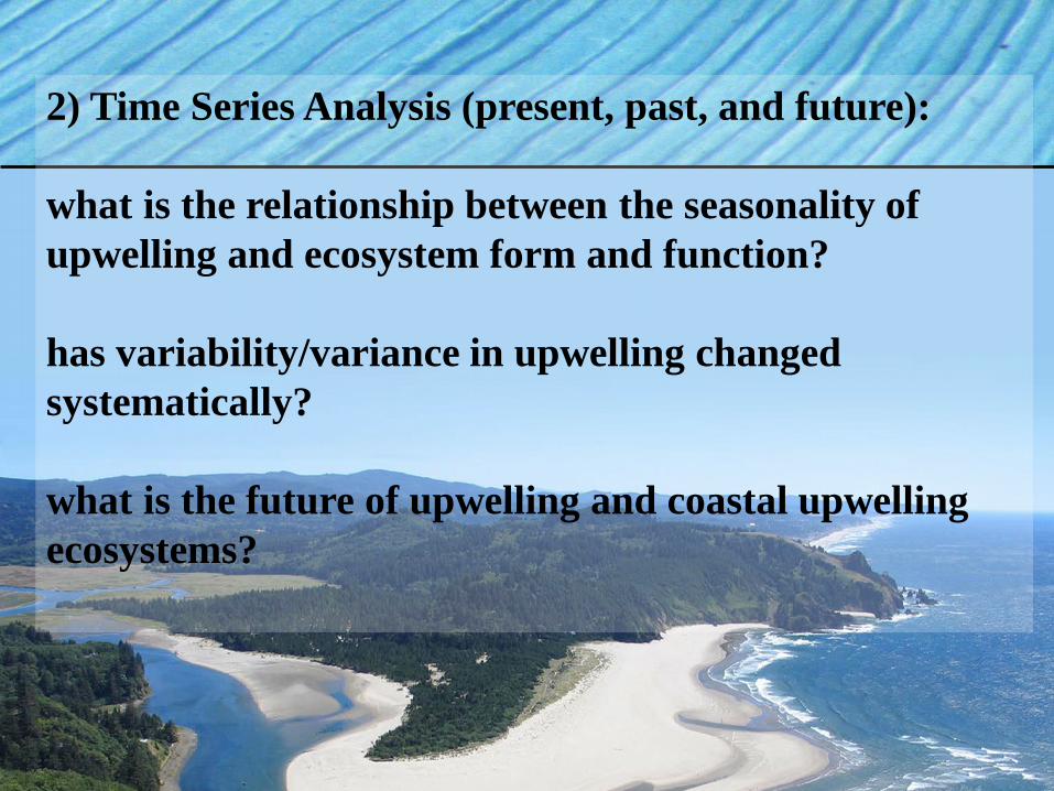
2) Time Series Analysis (present, past, and future): what is the relationship between the seasonality of upwelling and ecosystem form and function? has variability/variance in upwelling changed systematically? what is the future of upwelling and coastal upwelling ecosystems?

Sebastes diploproa, splitnose rockfish

Photo credit:Lifted from M. Love’s webpage

80+ yrs old 300 m depth Collections 1980 – 2008 1 of ~60 species in the region

Groundfish Growth: Splitnose rockfish (Sebastes diploproa)

region of strongest upwelling in CCS

Annual growth increments analogous to trees

1933: year of birth

1989: year of capture

Splitnose otolith

1983 El Nino

1958 El Nino

Master chronology

Splitnose chronology: 72 otoliths

Year

1920 1940 1960 1980 2000

Rin

g w

idth

inde

x

0.4

0.6

0.8

1.0

1.2

1.4

1.6

valid: 36 to 40 degrees latitude

Cross-correlations with upwelling index @ 39N Splitnose rockfish chronology and monthly upwelling (51 yrs)

wintertime (JF) upwelling has strongest effect; no effect seen

during the peak of annual cycle of upwelling

Month

JUL-prev

AU

G-prev

SE

P-prev

OC

T-prev

NO

V-prev

DE

C-prev

JAN

FEB

MA

R

AP

R

MAY

JUN

JUL

AU

G

SE

P

OC

T

NO

V

DE

C

Cor

rela

tion

coef

ficie

nt

-0.1

0.0

0.1

0.2

0.3

0.4

0.5

0.6

* p < 0.01 * *

yelloweye rockfish piscivorous

Covariance between fish and seabirds?

splitnose rockfish planktivorous

growth-increment chronologies

common murre piscivorous

Cassin’s auklet planktivorous

egg-laying dates

and

breeding success

Chinook salmon piscivorous

Sub-annual scale of responses

Biotic time series

lay date (julian day)

120 130 140 150 160 170

lay date (julian day)

80 100 120 140 160

success

0.0 0.2 0.4 0.6 0.8 1.0

success

0.0 0.2 0.4 0.6 0.8 1.0 1.2

ring width index

0.7 0.8 0.9 1.0 1.1 1.2

year

0.7 0.8 0.9 1.0 1.1 1.2

murre lay date

auklet lay date

murre success

auklet success

splitnose chronology

1950 1960 1970 1980 1990 2000 2010

ring

wid

th in

dex

-1.0

-0.5

0.0

0.5 1.0 yelloweye chronology

salmon chronology

ring width index

lay date fledgling success

growth-increm

ent chronology

Biotic time series: mostly winter correlations

corr

elat

ion

coef

ficie

nt (r

)

-0.8

-0.6

-0.4

-0.2

0.0

0.2

0.4

0.6

0.8

murre hatch auklet hatch murre success auklet success

month

JUL-prev

AUG

-prev SEP-prev O

CT-prev

NO

V-prev D

EC-prev

JAN

FEB M

AR

APR

MAY

JUN

JU

L AU

G

SEP O

CT

NO

V D

EC

correlation coefficient (r)

-0.6

-0.4

-0.2

0.0

0.2

0.4

0.6

yelloweye splitnose salmon

Combining biotic time series

lay date (seabirds)

breeding success (seabirds)

growth (rockfish, salmon)

lay date (julian day)

120 130 140 150 160 170

lay date (julian day)

80 100 120 140 160

success

0.0 0.2 0.4 0.6 0.8 1.0

success

0.0 0.2 0.4 0.6 0.8 1.0 1.2

ring width index

0.7 0.8 0.9 1.0 1.1 1.2

year

0.7 0.8 0.9 1.0 1.1 1.2

murre lay date

auklet lay date

murre success

auklet success

splitnose chronology

1950 1960 1970 1980 1990 2000 2010

ring

wid

th in

dex

-1.0

-0.5

0.0

0.5 1.0 yelloweye chronology

salmon chronology

common interval: 1978 - 2001

ring width index

Multivariate response variable (EOF of biotic series)

PCA axis 1

0.10 0.15 0.20 0.25

PC

A ax

is 2

-0.4

0.0

0.4

0.8

salmon

auklet success

yelloweye

splitnose

murre success

murre date

auklet date

EOF1 and EOF2 fish and bird vs. upwelling: winter sensitive and summer sensitive spp.

PC

1

-4 -3 -2 -1 0 1 2

Year 1975 1980 1985 1990 1995 2000 2005

Cor

rela

tion

coef

ficie

nt

-0.4

-0.2

0.0

0.2

0.4

0.6

Month

JUL-prev

AU

G-prev

SE

P-prev

OC

T-prev N

OV-prev

DE

C-prev

JAN

FE

B

MA

R

AP

R

MAY

JU

N

JUL

AU

G

SE

P

OC

T N

OV

D

EC

* p < 0.01 *

Month

JUL-prev

AU

G-prev

SE

P-prev

OC

T-prev N

OV-prev

DE

C-prev

JAN

FE

B

MA

R

AP

R

MAY

JU

N

JUL

AU

G

SE

P

OC

T N

OV

D

EC

Cor

rela

tion

coef

ficie

nt

-0.4

-0.2

0.0

0.2

0.4

0.6 * p < 0.01 *

59% variance explained; eigenvalue = 4.1

3

Year 1975 1980 1985 1990 1995 2000 2005

PC

2

-3 -2 -1 0 1 2

16% variance explained; eigenvalue = 1.1

Species Winter/Spring Summer Location Variable Cassin’s Auklet + + + + + Farallon Islands Lay Date Common Murre + + + + + Farallon Islands Lay Date

Cassin’s Auklet + + + + Farallon Islands Repro. success

Common Murre + + + Farallon Islands Repro. success

Rhinoceros Auklets + Farallon Islands Repro. success

Pigeon Guillemot + Farallon Islands Repro. success Pelagic Cormorant + Farallon Islands Repro. success Brandt’s Cormorant + Farallon Islands Repro. success

Brandt’s Cormorant + Farallon Islands Survival

Rhinoceros Auklets + Año Nuevo Repro. success

Splitnose Rockfish + + + + N California Otolith crn.

Yelloweye Rockfish + + + + N California Otolith crn.

Aurora Rockfish + Oregon Otolith crn.

Chinook Salmon + + N California Scale crn.

Pacific Sardine + S California Recruitment

Krill + Central CA Abundance

Chlorophyll-a + Central CA Concentration

+ Schroeder et al. 2009 + Black et al. 2010 + Black et al. 2011 + Garcia-Reyes et al. 2013 + Schroeder et al. 2013 + Garcia-Reyes et al. 2014 (but only data in the summer for krill)

Environment: EOF of SST, wind, and UI

Winds and temps from 12 buoys 1988-2010 Upwelling from same latitudes

Early season environment explains biotic response

PCenv from winds, temps (winter / early spring signal) PCbio from 9 time series (56% variability explained)

R2 = 0.79 20 years

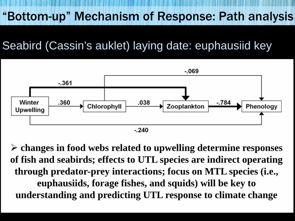
“Bottom-up” Mechanism of Response: Path analysis

Seabird (Cassin’s auklet) laying date: euphausiid key

changes in food webs related to upwelling determine responses of fish and seabirds; effects to UTL species are indirect operating through predator-prey interactions; focus on MTL species (i.e.,

euphausiids, forage fishes, and squids) will be key to understanding and predicting UTL response to climate change

Other Mechanisms of Response

Monthly matrix of Upwelling Index at 39N year JAN FEB MAR APR MAY JUN JUL AUG SEP OCT NOV DEC

1946 6 -10 45 36 85 111 140 155 35 59 5 -5

1947 14 -3 2 60 68 122 83 169 81 9 44 1

1948 -4 49 28 7 47 108 148 117 54 12 7 7

1949 40 22 -4 44 67 165 160 74 41 65 -35 11

1950 24 -7 12 72 210 121 205 90 48 -6 0 -58

1951 7 2 90 66 87 170 203 179 33 12 -18 4

1952 -3 2 104 45 100 137 144 126 52 0 0 -45

1953 -39 65 40 42 74 189 174 53 33 20 -23 8

. . . . . . . . . . . . .

. . . . . . . . . . . . .

. . . . . . . . . . . . .

2000 -21 -113 105 21 116 216 302 272 115 64 14 -5

2001 -5 -5 86 127 256 326 365 203 106 91 -12 -18

2002 3 0 33 117 202 388 271 285 130 129 -2 -175

2003 -102 37 20 18 221 302 327 154 140 51 -6 -95

2004 -38 -25 92 73 149 241 145 97 173 45 78 3

2005 -17 4 18 80 64 196 216 209 194 82 40 -37

2006 1 27 0 30 170 202 297 243 170 116 29 4

2007 107 23 112 146 239 228 116 138 105 37 56 26

2008 -1 39 133 150 231 287 170 194 87 65 11 34

-3

Upwelling 39N

winter mode PC1

JAN

FEB

MA

R

AP

R

MAY

JUN

JUL

AU

G

SE

P

OC

T

NO

V

DE

C

correlation coefficient (r)

-0.4 -0.2 0.0 0.2 0.4 0.6 0.8 1.0

PC2

Year 1940 1950 1960 1970 1980 1990 2000 2010

winter mode

Upw

ellin

g P

C1

-2 -1 0 1 2 3 PC1

25% variance explained

summer mode

Winter (Jan:Mar) upwelling index

-150 -100 -50 0 50 100

Sum

mer

(Jun

:Aug

) upw

ellin

g in

dex

50

100

150

200

250

300

350

winter vs. summer UW summer upwelling

3

Year 1940 1950 1960 1970 1980 1990 2000 2010

Upw

elling PC

2

-3 -2 -1 0 1 2

PC2

14% variance explained

winter upwelling

Scaling up: EOF of Upwelling Index across CCS

45N

42N

39N

36N

33N

% var 14 16 14 19 19

EV 1.68 1.87 1.71 2.24 2.22

winter mode

Correl. -0.01 -0.01 0.02 -0.08 -0.02

winter vs. summer

Principal components repeated at 5 locations

Lat 45 N 42 N 39 N 36 N 33 N

% var 15 24 25 30 34

EV 1.74 2.88 3.03 3.61 4.08

summer mode

EV = eigenvalue % var = percent variance explained

Trends in Seasonal Upwelling Index

Year 1950 1960 1970 1980 1990 2000 2010

Nor

mal

ized

inde

x

-2

0

2

4 summer mode (increase?)

45N

42N

39N

36N

33N J F M A M J J A S O N D

Latit

ude

Month

Year 1950 1960 1970 1980 1990 2000 2010

Norm

alized index -2

0

2

4 winter mode (variation)

45N

42N

39N

36N

33N J F M A M J J A S O N D

Latit

ude

Month

Coastwide analysis (5 upwelling stations)

Driver? Winter mode and sea level pressure

-4 -2 0 2

Nor

mal

ized

win

ter u

pwel

ling

-4

-3

-2

-1

0

1

2

3

NPH NOI

Normalized NOI, NPH

Winter mode vs. NOI and NPH

North Pacific High

Northern Oscillation Index

Correlation with winter sea level pressure

correlation coefficient (r)

Summer mode and sea level pressure

Correlation with summer sea level pressure

correlation coefficient (r)

Summer mode vs. NOI and NPH

Normalized NPH, NOI -3 -2 -1 0 1 2 3

Nor

mal

ized

sum

mer

upw

ellin

g

-3

-2

-1

0

1

2

3

NPH NOI

drivers of summer upwelling poorly understood

Ecosystem “preconditioning”, North Pacific High

Position (dots) and area of the NPH

Winter mode and the North Pacific High

pCUI = sum of all positive daily upwelling values (Jan-Feb)

R2 = 0.64

R2 = 0.57

Why winter?

Greatest variability Lengthen growing season Pre-condition (“jump start”) food web dynamics

North Pacific Current

But, also more than upwelling… source waters?

Winter NPH: Key to the past and Q: Has Upwelling Become more Variable?

correlation coefficient (r)

Jet stream

H

Reconstructing the Past Upwelling

Year

1900 1920 1940 1960 1980 2000

Norm

alize

d in

dex

-4

-2

0

2

4winter SLPwinter sea level

winter UWwinter climate

Year

1900 1920 1940 1960 1980 2000No

rmal

ized

inde

x-4

-2

0

2

4SLPwinter sea level

winter UW

Winter blocking high Correlation between upwelling and winter sea level pressure

correlation coefficient (r)

Jet stream

H storm track

Inverse correlation between NW winds, precip

Year

1900 1920 1940 1960 1980 2000No

rmal

ized

inde

x-4

-2

0

2

4 winter SLPwinter sea level

winter UWwinter climatewinter precip

Tree-ring chronology locations

Marine and terrestrial linkages

Year

1900 1920 1940 1960 1980 2000

Norm

alize

d in

dex

-4

-2

0

2

4treeswinter SLPwinter sea level

winter UWwinter climatewinter precip

Trees-3 -2 -1 0 1 2

Win

ter c

limat

e

-4

-3

-2

-1

0

1

2

R2 = 0.65

Running standard deviation

Year

1950 1960 1970 1980 1990 2000 2010

Nor

mal

ized

inde

x

-4

-3

-2

-1

0

1

2

3

Winter climate 1948-1968 1949-1969 1950-1970

Running standard deviation

Year

1950 1960 1970 1980 1990 2000 2010

Run

ning

std

dev

0.6

0.7

0.8

0.9

1.0

1.1

1.2

1.3

Winter climate

Running standard deviation

Year

1900 1920 1940 1960 1980 2000

Run

ning

std

dev

0.4

0.6

0.8

1.0

1.2

1.4 Sea levelWinter climate

Running standard deviation

SFO sea level

1880 1900 1920 1940 1960 1980 2000S

td. d

ev.

0.4

0.8

1.2

1.6winter climate

reconstruction

Year

1500 1600 1700 1800 1900 2000

Std

. dev

.

0.4

0.8

1.2

1.6

90% CI 95% CI

Future changes

Present

Future

S

Meta-analysis of literature: winds across EBCS

SL P

ress

ure

(hPa

)

1000

10

25

1015

10

20

1010

10

05

CON

SIST

ENCY

S

Meta-analysis: winds

Benguela California

Canary

Humboldt

Iberian

Stre

ngth

enin

g W

eake

ning

S

treng

then

ing

Wea

keni

ng