of cohesive zones on small faults and implications for ... · Effects of cohesive zones on small...

$: of cohesive zones on small faults and implications for ... · Effects of cohesive zones on small faults and implications for secondary fracturing and fault ... mal mineralization$
Pergamon Journalof Structural Geology, Vol. 19, No. 6, pp. 835 to 847, 1997

0 1997 Elsevier Science Ltd All rights reserved. Printed in Great Britain

PII: S0191-8141(97)00002-3 0191~8141197 $17.00+0.00

Effects of cohesive zones on small faults and implications for secondary fracturing and fault trace geometry

STEPHEN J. MARTEL

Department of Geology and Geophysics, University of Hawaii, 2525 Correa Road, Honolulu, HI 96822, U.S.A.

(Received 8 July 1996; accepted in revisedform 10 December 1996)

Abstract-Fracture mechanics theory and field observations together indicate that the shear stress on many faults is non-uniform when they slip. If the shear stress were uniform, then: (a) a physically implausible singular stress concentration theoretically would develop at a fault end; and(b) a single curved ‘tail fracture’ should open up at the end of every fault trace, intersecting the fault at approximately 70”. Tail fractures along many small faults instead range in number, commonly form behind fault trace ends, have nearly straight traces and intersect a fault at angles less than 50”. A ‘cohesive zone’, in which the shear stress is elevated near the fault end, can eliminate the stress singularity and can account for the observed orientation, shape, and distribution of tail fractures. Cohesive zones also should cause a fault to bend. If the cohesive zone shear stress were uniform, then the distance from the fault end to the bend gives the cohesive zone length. The nearly straight traces of the tail fractures and the small bends observed near some fault ends implies that the faults slipped with low stress drops, less than 10% of the ambient fault-parallel shear stress. 0 Elsevier Science Ltd

INTRODUCTION

Faults play key roles in a variety of processes in the

Earth’s crust. They produce some of nature’s most destructive phenomena and accommodate tremendous deformations in the Earth’s crust over geological time. They also are key pathways for the flow of water, petroleum, magma, geothermal fluids, and hydrothermal fluids (Goyal and Kassoy, 1980; Sibson, 1981; Bodvars- son et al., 1982; Stierman, 1984; Bruhn and Yonkee, 1988; McCaig, 1988; National Research Council, 1990, 1996; Forster and Evans, 1991; Antonellini and Aydin, 1994; Hickman et al., 1995). For both academic and practical reasons, faults have attracted the attention of many people, including many who are not geologists or seismologists.

Observations along exhumed faults provide informa- tion on faulting processes at depth that is difficult to obtain by other means. Measurements on exhumed faults commonly are coarser than those obtained in controlled experiments on shear fractures in the laboratory (e.g. Lockner et al., 1991; Blanpied et al., 1995), but exhumed faults reveal the effects of faulting under environmental conditions and at a size scale that are difficult to reproduce in the laboratory. Progress in electromagnetic methods (Black et al., 1991) and seismological techniques (e.g. Gillard ef al., 1995) allow ever smaller structures to be resolved along faults, but in few cases can the fine structure or composition of a fault be determined as accurately as direct observation allows.

Recurring field observations of exhumed faults and predictions of faulting models must be reconcilable if they both are to be used with confidence to understand faulting processes at seismogenic depths or to better predict fluid flow along faults. For example, hydrother-

mal mineralization and alteration along secondary fractures near the ends of fault traces consistently indicate that these fractures form excellent conduits for

fluid flow (Sibson, 1981; Segall and Pollard, 1983a). Even where the faults and fractures are ‘sealed’, hydraulic tests demonstrate that these seals are incomplete (e.g. Niva et al., 1988; Black et al., 1991); in some cases fluid flow can be observed directly along filled secondary fractures (Martel and Peterson, 1991). Secondary fractures can link originally unconnected faults, and as a result they will play a critical role in the hydraulic behavior of a fault system (Long and Witherspoon, 1985). Processes that form secondary fractures along faults thus are critically important to the hydraulic conductivity of fault systems, even where those fractures become partially sealed.

This paper deals specifically with field observations of secondary fracturing along faults and predictions of two- dimensional elastic fracture mechanics theory. Standard linear elastic fracture mechanics (LEFM) theory predicts that the stresses near the tip of a fault are singular, with the near-tip stresses having a characteristic form. These outcomes have two key difficulties as applied to observations of secondary fractures along exhumed faults. First, real materials cannot sustain infinite stress levels. Second, the characteristic form of the singular near-tip solution leads to predictions about secondary fracture distributions that are inconsistent with numerous field observations. For example, multiple secondary fractures commonly open near, but not precisely at, the ends of fault traces (Fig. 1). In other cases, secondary fractures are absent (e.g. Segall and Pollard, 1983a). Where secondary fractures do occur, they commonly form an angle of 50” or less with the fault trace. In contrast, conventional LEFM theory suggests that a single fracture should open precisely at the end of a fault trace

835

836 S. J. MARTEL

a Foliation *, FAULT _

Y

Secondary fractures

I I I I I I

0 5m

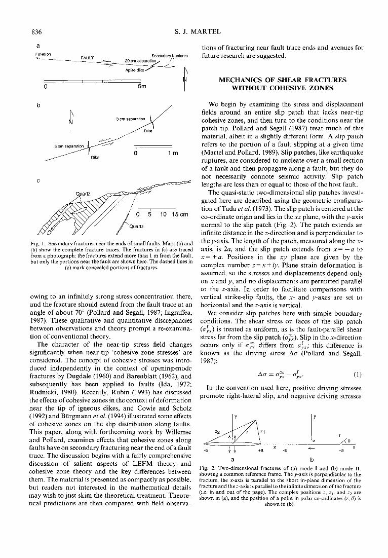
Fig. 1. Secondary fractures near the ends of small faults. Maps (a) and (b) show the complete fracture traces. The fractures in (c) are traced from a photograph; the fractures extend more than 1 m from the fault, but only the portions near the fault are shown here. The dashed lines in

(c) mark concealed portions of fractures.

owing to an infinitely strong stress concentration there, and the fracture should extend from the fault trace at an angle of about 70” (Pollard and Segall, 1987; Ingraffea, 1987). These qualitative and quantitative discrepancies between observations and theory prompt a re-examination of conventional theory.

The character of the near-tip stress field changes significantly when near-tip ‘cohesive zone stresses’ are considered. The concept of cohesive stresses was intro- duced independently in the context of opening-mode fractures by Dugdale (1960) and Barenblatt (1962) and subsequently has been applied to faults (Ida, 1972; Rudnicki, 1980). Recently, Rubin (1993) has discussed the effects of cohesive zones in the context of deformation near the tip of igneous dikes, and Cowie and Scholz (1992) and Btirgmann et al. (1994) illustrated some effects of cohesive zones on the slip distribution along faults. This paper, along with forthcoming work by Willemse and Pollard, examines effects that cohesive zones along faults have on secondary fracturing near the end of a fault trace. The discussion begins with a fairly comprehensive discussion of salient aspects of LEFM theory and cohesive zone theory and the key differences between them. The material is presented as compactly as possible, but readers not interested in the mathematical details may wish to just skim the theoretical treatment. Theore- tical predictions are then compared with field observa-

tions of fracturing near fault trace ends and avenues for future research are suggested.

MECHANICS OF SHEAR FRACTURES WITHOUT COHESIVE ZONES

We begin by examining the stress and displacement fields around an entire slip patch that lacks near-tip cohesive zones, and then turn to the conditions near the patch tip. Pollard and Segall (1987) treat much of this material, albeit in a slightly different form. A slip patch refers to the portion of a fault slipping at a given time (Martel and Pollard, 1989). Slip patches, like earthquake ruptures, are considered to nucleate over a small section of a fault and then propagate along a fault, but they do not necessarily connote seismic activity. Slip patch lengths are less than or equal to those of the host fault.

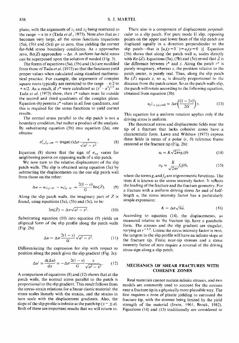
The quasi-static two-dimensional slip patches investi- gated here are described using the geometric configura- tion of Tada et al. (1973). The slip patch is centered at the co-ordinate origin and lies in the xz plane, with they-axis normal to the slip patch (Fig. 2). The patch extends an infinite distance in the z-direction and is perpendicular to the y-axis. The length of the patch, measured along the x- axis, is 2a, and the slip patch extends from x = -a to x= + a. Positions in the xy plane are given by the

complex number z=x+ iy. Plane strain deformation is assumed, so the stresses and displacements depend only on x and y, and no displacements are permitted parallel to the z-axis. In order to facilitate comparisons with vertical strike-slip faults, the x- and y-axes are set to horizontal and the z-axis is vertical.

We consider slip patches here with simple boundary conditions. The shear stress on faces of the slip patch (a;,) is treated as uniform, as is the fault-parallel shear stress far from the slip patch (a$). Slip in the x-direction occurs only if g,“X differs from &; this difference is known as the driving stress Aa (Pollard and Segall, 1987):

AC = c? - c&. YX (1)

In the convention used here, positive driving stresses promote right-lateral slip, and negative driving stresses

IY IY

22 z 21 49 r - //qe

x x -a +a -a

-h- +a

a b

Fig. 2. Two-dimensional fractures of (a) mode I and (b) mode II, showing a common reference frame. The y-axis is perpendicular to the fracture, the x-axis is parallel to the short in-plane dimension of the fracture and the z-axis is parallel to the infinite dimension of the fracture (i.e. in and out of the page). The complex positions z, zt, and z2 are shown in (a), and the position of a point in polar co-ordinates (r. 0) is

shown in (b).

Cohesive zones on small faults 837

Fig. 3. Boundary conditions for a slip patch of length 2a without cohesive zones. The net boundary conditions (c) reflect a superposition of (a) the far-field shear stress and (b) the negative of the driving stress for the slip patch. The lengths and directions of the arrows reflect the

relative magnitudes and signs of the shear stress, respectively.

promote left-lateral slip. Only sliding of slip patch walls (mode II displacement) is admitted; opening of fracture walls (mode I displacement) is not, so dilation of material in a fault is neglected. Uniform loading of a slip patch is considered by superposing two contributions (Fig. 3):

(1) a uniform shear stress 0; that acts both along the patch walls and at a distance far from the patch;

(2) a uniform shear stress & - 0~4: that acts along the slip patch (Ix] 5 a) in a body subject to no far-field stresses. The shear stress along the slip patch walls is the negative of the driving stress.

Both contributions are necessary to recover the complete stress field, but only the latter contributes to the displacement field associated with fault slip.

Closed-form analytical solutions for the two-dimensional stress and displacement fields around a slip patch are obtained here from complex stress functions (Tada et al., 1973; Pollard and Segall, 1987). Complex stress functions in some ways provide more direct physical insight into the deformation around a slip patch than other methods, such as singular integral equation formulations (Barber, 1992; Hills et al., 1996) or conformal mapping (Muskhelishvilli, 1953). They also have a key advantage over numerical methods such as constant displacement-discontinuity boundary element techniques (Crouch and Starfield, 1974) in that the stresses and displacements can be calculated at points arbitrarily close to the patch walls. The following discussion of complex stress functions goes into some detail to provide complete solutions and to develop the insight that these functions can provide.

The stress components (rrXX, ovv, cXY and a,,,.) and the displacement components (u, and uJ depend on three complex functions (2, Z and Z’) of position z (Tada et al., 1973). For pure mode II fracturing, the stresses and displacements are:

0 - 2 Im(Z) + XX - y Re(Z’) (2a)

c7 ,,y = -y Re(.Z’) (2b)

a,.. = aYX = Re(Z) + y Im(Z’) (2c)

u, = [2( 1 - u) Im(Z) + y Re(Z)]/2G (3a)

u,, = [-( 1 - 2~) Re(Z) + y Im(Z)]/2G. (3b)

Here u is Poisson’s ratio and G is the shear modulus. The stress functions are related to each other through their derivatives:

Z,dz dz

ze. (44

A few useful general points can be made here about the

stress functions, even without knowing their specific forms. First, the stresses (equations (2a1, (2b) and (2~)) depend on Z and Z’ (and not on Z), whereas the displacements (equations (3a) and (3b)) depend on Z and Z, but not on Z’. This should be the case given the relationships of equations (4a) and (4b): the stresses, determined by Z and Z’, are proportional to strains, and the strains must be integrated to determine displacements. Second, equations (2a), (2b) and (2~) show that the real and imaginary parts of Z’ must go to zero as y increases in order that the far-field stresses remain finite far from the slip patch. Third, on the slip patch face, where 1x1 5 a and y=O, the above expressions simplify significantly and yield the stresses on the slip patch faces. The latter two points allow the stress functions to be identified with the boundary conditions for the problem.

The stress functions for a uniformly loaded slip patch under no far-field stresses are (Tada et al., 1973):

Z = Aa[z* - z] (sa)

Z=AaL-1 [ 1 Z*

(5b)

Z’=Aa A, [ 1 (5c)

where

and

zI=JzI&

zi =z-a

(6)

(74

z2 =z+a. O’b)

In equations (7a) and (7b), zr is the position of a point relative to the positive end of the slip patch, and z2 is the position relative to the negative end of the patch (Fig. 2). Note that z1 and z3 can lie in anv auadrant of the comnlex

838 S. J. MARTEL

plane, with the arguments of z1 and z2 being restricted to the range --71 to 7~ (Tada et al., 1973). Note also that as z becomes very large, all the stress functions (equations (5a), (5b) and (5~)) go to zero, thus yielding the correct far-field stress boundary conditions. As z approaches zero, Re(2) approaches - Aa. A uniform far-field stress can be superposed upon the solution if needed (Fig. 3).

The forms of equations (5a), (5b) and (5~) are modified from those of Tada et al. (1973) so that the functions yield

proper values when calculated using standard mathematical practice. For example, the arguments of complex square roots typically are restricted to the range -n/2 to + 71/2. As a result, if z* were calculated as (~~-a~)“~ as Tada et al. (1973) show, then z* values must lie outside the second and third quadrants of the complex plane. Equation (6) permits z* values in all four quadrants, and this is required for the stress functions to yield correct results.

The normal stress parallel to the slip patch is not a boundary condition, but rather a product of the analysis. By substituting equation (5b) into equation (2a), one obtains:

Equation (8) shows that the sign of oXX varies for neighboring points on opposing walls of a slip patch.

We now turn to the relative displacement of the slip patch walls. The slip is obtained using equation (3a) by subtracting the displacements on the one slip patch wall from those on the other:

Au = u,]~__~+ - u,jY=s- = 2(1 - u) ~ Im(g). G (9)

Along the slip patch walls, the imaginary part of 2 is found, using equations (5a), (5b) and (5c), to be:

Im(z) = Aam. (10)

Substituting equation (10) into equation (9) yields an elliptical form of the slip profile along the patch walls (Fig. 2b):

Differentiating the expression for slip with respect to position along the patch gives the slip gradient (Fig. 2~):

Au, = 4A4 _Aow - 4 x -zz

dx G ,/m’ (12)

A comparison of equations (8) and (12) shows that at the patch walls, the normal stress parallel to the patch is proportional to the slip gradient. This result follows from the stress-strain relations for a linear elastic material: the stress scales linearly with the strains, and the strains in turn scale with the displacement gradients. Also, the slope of the slip profile is infinite at the patch tip (x = + a). Both of these are important results that we will return to.

There also is a component of displacement perpendicular to a slip patch. For pure mode II slip, opposing points on the upper and lower faces of the slip patch are displaced equally in a direction perpendicular to the slip patch-that is [u& = 0’) = z+,(v = O-)]. Equation (3b) shows that along the patch wall uv scales directly with Re (2). Equations (5a), (5b) and (5~) reveal that 2 is the difference between z* and z. Along the patch z* is purely imaginary, whereas z, the position relative to the

patch center, is purely real. Thus, along the slip patch Re (2) equals z, so uY is directly proportional to the

distance from the patch center. So as the patch walls slip, the patch will rotate according to the following equation, obtained from equation (3b):

x. (13)

This equation for a uniform rotation applies only if the driving stress is uniform.

The theoretical stress and displacement fields near the tip of a fracture that lacks cohesive zones have a characteristic form. Lawn and Wilshaw (1975) express these fields in terms of a polar (Y, 6) reference frame centered at the fracture tip (Fig. 2b):

pi = KdGgi(O) (14)

Oij = &j(O)3 (15)

where the terms gi and fV are trigonometric functions. The term K is known as the stress intensity factor. It reflects the loading of the fracture and the fracture geometry. For a fracture with a uniform driving stress AC and of half- length a, the stress intensity factor has a particularly simple expression:

K = Aa&. (16)

According to equation (14) the displacements, as measured relative to the fracture tip, have a parabolic form. The stresses and the slip gradient are singular, varying as r -‘I2 Unless the stress intensity factor is zero, . the tangent to the slip profile will have an infinite slope at the fracture tip. Finite near-tip stresses and a stress intensity factor of zero require a reversal of the driving stress sign along a slip patch.

MECHANICS OF SHEAR FRACTURES WITH COHESIVE ZONES

Real materials cannot sustain infinite stresses, and two models are commonly used to account for the stresses near a fracture tip in a physically more plausible way. The first requires a zone of plastic yielding to surround the fracture tip, with the stresses being limited by the yield strength of the material (Irwin, 1961; Broek, 1982). Equations (14) and (15) traditionally are considered to


Fig. 4. Boundary conditions for a slip patch of length 2a with cohesive zones of length R at the slip patch ends. The boxes at the ends of the slip patch border the cohesive zones. The net boundary conditions (d) reflect a superposition of (a) the far-field shear stress, (b) the negative of the driving stress associated with the central portion of the slip patch and (c)

the negative of the driving stress associated with the cohesive zones.

apply outside this small region (e.g. Rice, 1968). In the second model, finite cohesive stresses occur in zones near the fracture ends to prevent a singularity in the fracture- tip stresses (Dugdale, 1960; Barenblatt, 1962; Ida, 1972; Palmer and Rice, 1973; Rudnicki, 1980).

A cohesive zone model for a slip patch is followed here (Fig. 4). The fault-parallel shear stress far from the fault again is o,“x, the shear stress in the cohesive zones is & and the shear stress along the slip patch outside of the cohesive zones is &This model can be envisioned as the superposition of three contributions:

(1) a uniform shear stress o$ that acts both along the patch walls and at a distance far from the patch;

(2) a uniform shear stress & -cry2 that acts over the central slip patch interval 1x1 ( a - R, with no shear stress acting in the interval a - R -C 1x1 5 a;

(3) a uniform shear stress c& -cry: that acts in two cohesive zones of length R that exist over the patch intervals a - R < (xl I a, with no shear stress acting in the central interval 1x1 5 a - R.

All three contributions are necessary to recover the stress field, but only the latter two contribute to the displacement field associated with fault slip. Along a real fault the cohesive zone shear stress is quite likely to differ from the step function distribution considered here, perhaps varying linearly with distance from the patch end. The stresses are held uniform here to present a cohesive zone model in its most simple form.

The complex stress functions for calculating the elastic fields arising from slip under a constant driving stress along part of a slip patch are (Tada et al., 1973, p. 5.11):

!

(z - c) sin-’ u2 - ” (z - b) sin _, u2-bz

~ z = ~ u(z - c) u(z - b)

n + sin-’ C _ sin-’

U I (174

Z’=E ?r

sin-’ u2 - cz . _, u2-bz

~ - ‘ln u(z - c) u(z - 6)

sin-’ z - sin- lb a >

(17b)

(17c)

The terms b and c delimit the negative and positive ends of an interval of uniform driving stress, so the above equations must be applied three times, once for each of the cohesive zones and once for the central portion of the slip patch. For example, for the left-hand cohesive zone in Fig. 4, b= --a and c= R-u.

The contribution of a given interval of uniform driving stress to the stress intensity factor is (Tada et al., 1973):

[ sin-’ f: _ sin-’

U ;+=izqbjll;;)l.

(18) If the dimensions of the two cohesive zones are related

to the driving stress levels in the following manner:

u-R CF-,c

sin-’ - YX YX - ( > U

@o-.~f -- YX .J= -, a-R

cos - ( >

(19)

U

then the stress intensity factor contributions from the central portion of the patch and the cohesive zones cancel each other to yield a total stress intensity factor of zero. Cohesive zones thus permit the stresses along a slip patch to be finite, and they allow the slip profile to taper asymptotically to zero near the patch tip rather than being parabolic (Fig. 5). The driving stress associated with cohesive zones described by equation (19) is opposite in sign to the driving stress associated with the remainder of theputch and refects resistance to slip (Fig. 4). Even if the cohesive zone shear stress differs from the uniform distribution considered here, the sign of the driving stress in at least part of a cohesive zone would be opposite that elsewhere along the slip patch to achieve a stress intensity factor of zero.

The stress and displacement fields around a slip patch with cohesive zones differ in some intriguing ways from a slip patch with a uniform driving stress. For example,

840 S. J. MARTEL

-10 L , .,

-0 6 -0.4 -0.2 0 0.2 0.4 0.6 0.6 1

-10 ’ I -1 -0 8 -0.6 -0.4 -0.2 0 0.2 0.4 0.6 0.6 1

10 C-I ‘,L,<

$ 0

-10 -1 -0.8 -0.6 -0.4 -0.2

Normalized positionkng s~~patch”&a) 0.6 0.6 1

of a cohesive zone.

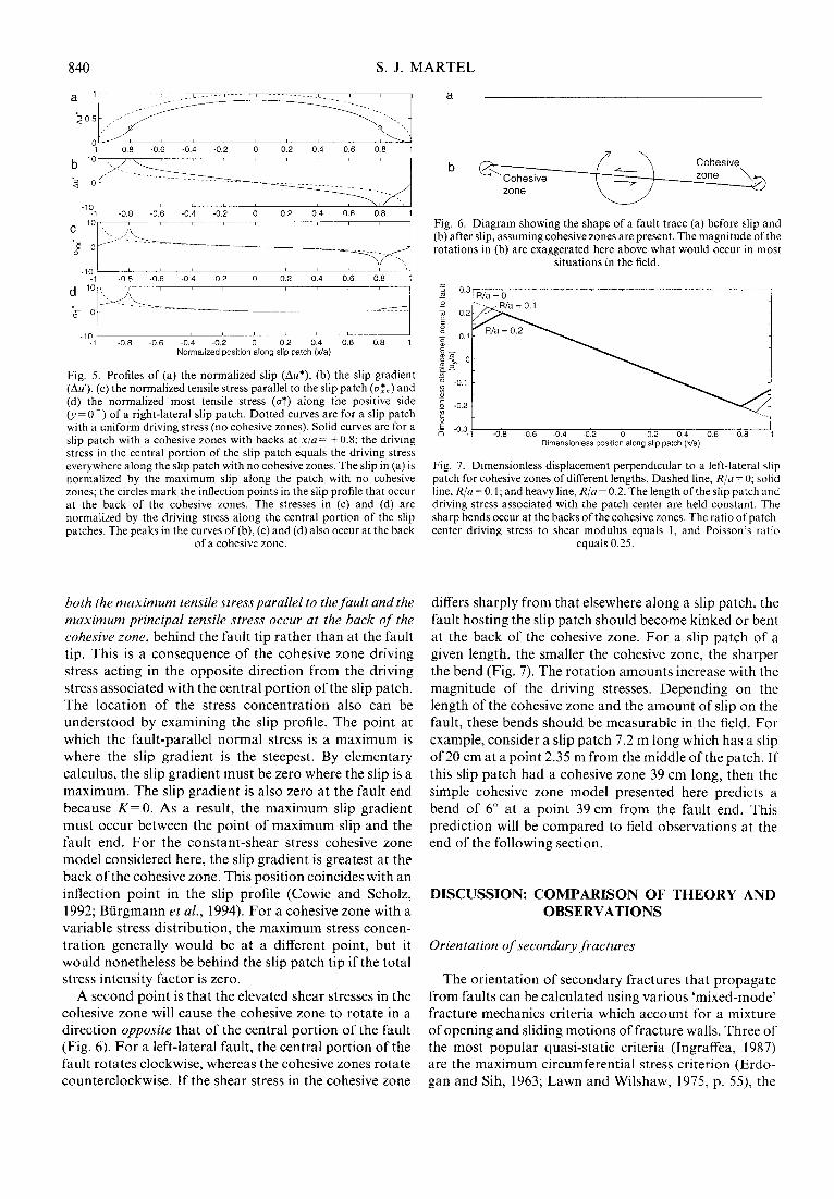
Fig. 5. Profiles of (a) the normalized slip (AU*), (b) the slip gradient (AU’), (c) the normalized tensile stress parallel to the slip patch (CT&) and (d) the normalized most tensile stress (UT) along the positive side (J = 0 ‘) of a right-lateral slip patch. Dotted curves are for a slip patch with a uniform driving stress (no cohesive zones). Solid curves are for a slip patch with a cohesive zones with backs at x/a = k 0.8; the driving stress in the central portion of the slip patch equals the driving stress everywhere along the slip patch with no cohesive zones. The slip in (a) is normalized by the maximum slip along the patch with no cohesive zones; the circles mark the inflection points in the slip profile that occur at the back of the cohesive zones. The stresses in (c) and (d) are normalized by the driving stress along the central portion of the slip patches. The peaks in the curves of(b), (c)and (d) also occur at the back

both the maximum tensile stress parallel to thefuult and the

maximum principal tensile stress occur at the buck of the cohesive zone, behind the fault tip rather than at the fault tip. This is a consequence of the cohesive zone driving stress acting in the opposite direction from the driving stress associated with the central portion of the slip patch. The location of the stress concentration also can be understood by examining the slip profile. The point at which the fault-parallel normal stress is a maximum is where the slip gradient is the steepest. By elementary calculus, the slip gradient must be zero where the slip is a maximum. The slip gradient is also zero at the fault end because K=O. As a result, the maximum slip gradient must occur between the point of maximum slip and the fault end. For the constant-shear stress cohesive zone model considered here, the slip gradient is greatest at the back of the cohesive zone. This position coincides with an inflection point in the slip profile (Cowie and Scholz, 1992; Btirgmann et al., 1994). For a cohesive zone with a variable stress distribution, the maximum stress concentration generally would be at a different point, but it would nonetheless be behind the slip patch tip if the total stress intensity factor is zero.

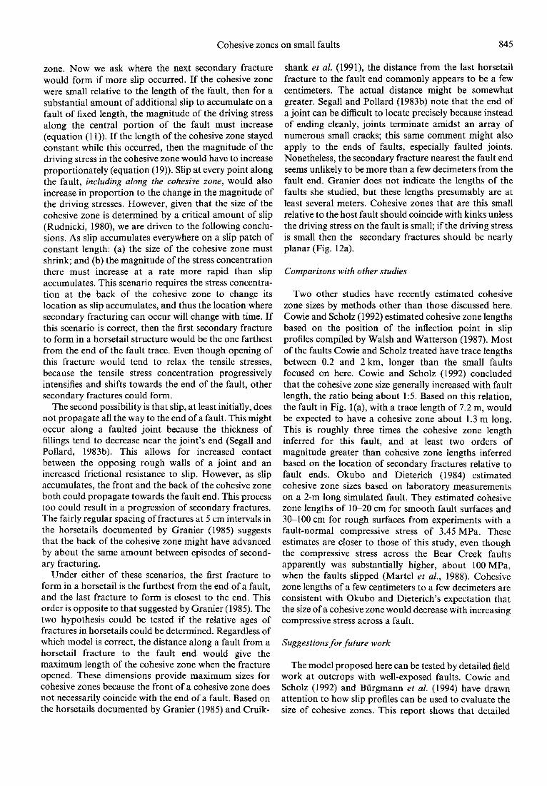
A second point is that the elevated shear stresses in the cohesive zone will cause the cohesive zone to rotate in a direction opposite that of the central portion of the fault (Fig. 6). For a left-lateral fault, the central portion of the fault rotates clockwise, whereas the cohesive zones rotate counterclockwise. If the shear stress in the cohesive zone

a

b c$k Cohesive ZO”e

Cohesive ZOW

Fig. 6. Diagram showing the shape of a fault trace (a) before slip and (b) after slip, assuming cohesive zones are present. The magnitude of the rotations in (b) are exaggerated here above what would occur in most

situations in the field.

4 E B -0.3.1 -0.8 -0.6 -0.4 -0 2 0 0.2 0 4 0.6 0.8

DImensionless posltion along slip patch (x/a)

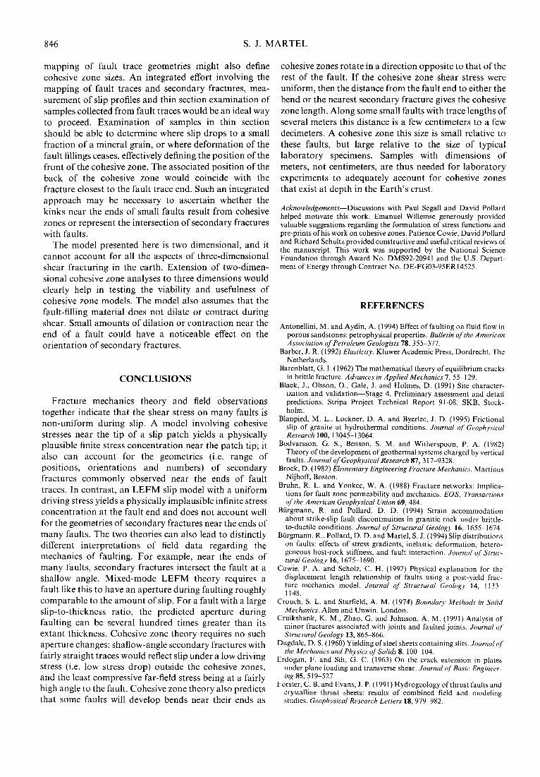
Fig. 7. Dimensionless displacement perpendicular to a left-lateral slip patch for cohesive zones of different lengths. Dashed line, R/a = 0; solid

equals 0.25.

line, R/a = 0.1; and heavy line, R/a = 0.2. The length of the slip patch and driving stress associated with the patch center are held constant. The sharp bends occur at the backs of the cohesive zones. The ratio of patch- center driving stress to shear modulus equals 1, and Poisson’s ratio

differs sharply from that elsewhere along a slip patch, the fault hosting the slip patch should become kinked or bent at the back of the cohesive zone. For a slip patch of a given length, the smaller the cohesive zone, the sharper the bend (Fig. 7). The rotation amounts increase with the magnitude of the driving stresses. Depending on the length of the cohesive zone and the amount of slip on the fault, these bends should be measurable in the field. For example, consider a slip patch 7.2 m long which has a slip of 20 cm at a point 2.35 m from the middle of the patch. If this slip patch had a cohesive zone 39 cm long, then the simple cohesive zone model presented here predicts a bend of 6” at a point 39 cm from the fault end. This prediction will be compared to field observations at the end of the following section.

DISCUSSION: COMPARISON OF THEORY AND OBSERVATIONS

Orientation of secondary fractures

The orientation of secondary fractures that propagate from faults can be calculated using various ‘mixed-mode’ fracture mechanics criteria which account for a mixture of opening and sliding motions of fracture walls. Three of the most popular quasi-static criteria (Ingraffea, 1987) are the maximum circumferential stress criterion (Erdo- gan and Sih, 1963; Lawn and Wilshaw, 1975, p. 55) the


0 20 40 60 80 100 120 140 160 180 Angle (‘)

Fig. 8. Angular dependence of circumferential stress (Erdogan and Sih, 1963), energy release rate (Hussain et al., 1974; Lawn and Wilshaw, 1975) and strain energy density (Sih, 1973) fracture propagation criteria about the tip of a uniformly loaded, two-dimensional, pure mode II fracture. Poisson’s ratio equals 0.25. Each function is normalized to a maximum value of 1 and calculated for a fixed small distance r from the fracture tip. The maximum values of the circumferential stress and the energy release rate, and the minimum value of the strain energy density,

all occur near 70”

1.5 a. , , , , , , , 1 ////////

0.5 """ //

//,,/ // /

0, - / /-/,c ;; '

-0.5

I_

, , / / ,/,' / / :/

_, / / / y,', / / 'y

, , ..,,', / / / i, -1.5 ,'

I

-I,,' 0 1 :

/ / / / / / / / , / / / , / /

0.9 1 1.1

Fig. 9. Trajectories of most compressive principal stress near a left- lateral slip patch with a uniform stress drop. The driving stress equals the far-field shear stress parallel to the fault (i.e. there is a complete stress drop). The angle of the most compressive far-field stress relative to the patch is (a) 45” and (b) 15”. Figures (c) and (d) show virtually identical

trajectory patterns inside the box surrounding the patch tip.

maximum energy release rate criterion (Hussain et al.,

1974; Lawn and Wilshaw, 1975, p. 68) and the minimum strain energy density criterion (Sih, 1973, 1974). These criteria usually are cast in terms of stress intensity factors and applied to fractures that are assumed to have no cohesive zones. For a uniformly loaded pure mode II slip patch (no fracture opening), all of these criteria predict that a secondary fracture should extend from a fault at an angle (u) of about 70” (Fig. 8). This angle is independent of the orientation of the principal compressive stress (p) far from the fault (Fig. 9) and the shear driving stress (Fig. 10). The predicted fracture angle increases with slip patch propagation speed (Freund, 1990).

Predictions of secondary fracture orientations based on pure mode II slip under uniform driving stresses do

1.5 a. , , , , , , / k ,U///////

0.5 """"

0 : *a,;

-0.5

/

/ / / / /,' / / ,;I

_, / / / ,p‘,, / / ;

-1.5 / / y" . ...,

,' -l,,' 0 1 : .'

' ' ' ' ' ' ' '

0.9 1 1.1

Fig. 10. Trajectories of most compressive principal stress near a left- lateral slip patch with a uniform stress drop. The driving stress equals 1% of the far-field shear stress parallel to the fault (i.e. there is a very low stress drop). The angle of the most compressive far-field stress relative to the patch is 45”, the same as in Fig. 9(a). Owing to the low driving stress, the stress trajectory pattern inside the box surrounding the patch tip is

different from the patterns in Figs IO(b) and 9(c),

not square well with field observations of many faults. Cruikshank et al. (1991) described CY angles between 35” and 50” for faulted joints in sandstone at Arches National Park. Segall and Pollard (1983a) reported angles of 15- 35” for secondary fractures near the ends of small faults (faulted joints) in granodiorite in the Bear Creek region of the Sierra Nevada in California. Angles of less than 50” have also been observed at the ends of small faults in granitic rocks in the Mt Pinchot quadrangle of the Sierra Nevada in California (Moore, 1963), near Grimsel Pass, Switzerland (Martel and Peterson, 1991) and in the Cevennes Mountains of France (Granier, 1985). The angles observed in the field are considerably lower than those predicted by a pure mode II model of faulting involving a uniform stress drop.

Cruikshank et al. (1991) used the maximum circumferential stress criterion in conjunction with a two-dimen-

sional mixed-mode LEFM model to account for the orientation of secondary fractures near the ends of small-displacement faults at Arches National Park. Cruikshank and his co-workers assumed that the faults were subject to uniform driving stresses, and that the secondary fractures opened perpendicular to the greatest circumferential stress (oes) near the fault tip. Based on these conditions, they then related the ratio of fault aperture (w) to slip (U) at the time of faulting to the angle c(. For a pure mode I fracture (W/U= a), ol=O”. For a pure mode II fracture (W/U=O), CI=COS-’ (1/3)~70.5”. These angles hold no matter how large the relative displacements of the fracture walls are, provided they are not zero. Cruikshank et al. attributed angles between 0”

842 S. J. MARTEL

and 70.5” to a mixture of opening and sliding of the fault walls. For angles between 35” and 50”, they calculated

that the ratio of opening to slip at the time of faulting was between 2 and 3 (Cruikshank et al., 1991, table 1). Based on this analysis, Cruikshank and his co-workers coined the ‘Moab Rule’: that the faulted joints at Arches had an initial aperture greater than or equal to the eventual amount of slip.

The Moab Rule encounters difficulty when applied to other faults however. For example, some of the faults along Bear Creek are only about 1 cm thick yet display 2 m of slip (Martel et al., 1988). These faults are spaced a

couple of meters apart and appear to have traces lengths of no more than a few hundred meters. The faults of Bear Creek resemble small faults elsewhere in the Sierra Nevada (Moore, 1963) and in Europe (e.g. Martel and Peterson, 1991). If the Moab Rule applied to faults in Bear Creek, then some would have had original apertures of 4-6 m, several hundred times their current thickness. An aperture change of this magnitude on the Bear Creek faults would require profound deformation in the surrounding rock and profound changes in the hydraulic behavior of the faults. The rocks adjacent to the faults are in general mildly deformed and do not show evidence of intense, widespread hydrothermal alteration. The major discrepancies between predictions of the Moab Rule and the observations at Bear Creek indicate that a mixed- mode slip model invoking a uniform driving stress neglects a key physical phenomenon that accompanies faulting in at least some rocks.

Before addressing the quantitative effect a cohesive zone would have on the orientation of a secondary fracture, we first review how a secondary fracture would form conceptually. It presumably nucleates where the greatest tensile stress concentration occurs. For the uniform-stress cohesive zone model adressed here, this point is at the back of a cohesive zone. The orientation of the fracture can be described in terms of two angles, a and /I, which are measured here relative to fault strike. The orientation of the most compressive stress at the back of a cohesive zone (a) gives the preferred orientation of a secondary fracture where it extends from the slip patch (Fig. 12c, inset). The fracture will tend to track the orientation of the local most compressive stress as it propagates (Ingraffea, 1987; Pollard and Segall, 1987; Biirgmann et al., 1994). If it propagates far enough, its tip will point in the direction of the far-field most compressive stress (p). Based on Figs 9-l 1 this should not require a secondary fracture to grow to a length greater than 0. l- 0.2a. If cI were equal to p, then a fracture would be planar and have a perfectly straight trace. If a exceeds p, then a fracture will curve.

Figure 12 shows the orientation of the most compressive stress (a) near the back of a cohesive zone as a function of the orientation of the most compressive far- field stress (8) for different driving stresses in a slip patch center. Figure 12(a-c) illustrates effects for cohesive zones of length O.OOla, 0.1~ and 0.2a, respectively. In

, , , , , , , / 0.5 """"

0.15r7;j o.15(i”: ; ,’ : : ; : 1 0.1 l////////j o,,~,,//,,,,j

I///,,,,. 0.05 0.05 ' ' ' ' ' ' ' '

0 l_i/ /////

__T,,,,,, 0 =/ ""' -7 N/,/X

-0.05 L _ _ , , , , , , 1 ;-r

-0.05 , , / , / / , , _

-;:I 1 ; : :, : : : : 1 .;;;I : ; : :_: : : : 1 0.9 1 1.1 0.9 1 1.1

Fig. I I. Trajectories of most compressive principal stress near a left- lateral slip patch with cohesive zones with backs at Ix/al = 0.9. The angle of the most compressive far-field stress relative to the patch is 15”. The driving stress at the patch center (relative to the far-field shear stress parallel to the patch) is (a) 100% and (b) 1%. The trajectory patterns inside the boxes surrounding the patch tip in (c) and (d) differ from each

other and those in Figs 9(c & d) & IO(b).

each of these figures, the line a=p corresponds to a condition where a slip patch has not perturbed the ambient stress field (i.e. the fault has not slipped). The line IX=B thus represents a lower limit for faulting, and hence secondary fractures cannot form such that a < /3. Unless the material in a fault can deform plastically under the ambient shear stress, a secondary fracture with a perfectly straight trace (i.e. c( = p) should not be able to form.

A long secondary fracture with a nearly straight trace generally would imply a very low driving stress (i.e. very low stress drop) on the central portion of a slip patch. Figure lZ(a-c) shows that if CI and /I differ by less than 5” (the interval between the two dashed lines), then for fractures with I angles between 10” and 50” the driving stress can be no more than O.l~,~.

The change in strike of a secondary fracture constrains the driving stress on the central portion of a slip patch. For example, consider a slip patch with a cohesive zone of length 0. la (Fig. 12b) intersected by a secondary fracture at an c( angle of 30”. If the tip of the fracture turned to a /3 angle of 24”, a driving stress of O.OloY$ is indicated, whereas if/J equals 8”, the driving stress would be 0.1~~:. Large changes in the strike of a secondary fracture thus imply a relatively large driving stress.

For very small cohesive zones (Fig. 12a) only very small driving stresses can account for most of the allowable range of permitted fracture orientations. For example, suppose the driving stress along the central portion of a slip patch were greater than 0.1 u,“x. Then, only if the far-field most compressive stress is at an


a a

1

Fig. 12. Predicted secondary fracture orientations as a function of the most compressive far-field stress for various driving stresses. The driving stresses are normalized relative to far-field shear stress. The uppermost curves are for the largest stress drops. The dashed line a = ,3 corresponds to a driving stress (i.e. stress drop) of zero, the lower limit of faulting. Faulting, and hence secondary fracturing, is not permitted for

OL </?. Cohesive zone lengths are (a) O.OOla, (b) O.la and (c)0.2a.

extremely shallow angle relative to the slip patch (i.e. /I < 2”) is an c( angle less than 80” permitted. Large driving stresses will invariably produce a secondary fracture that

intersects a fault at a high angle. This can be understood

by considering the limiting case of a slip patch with a cohesive zone of zero length: in this case secondary fractures would emerge at angles of about 70” under any non-zero driving stress. An extremely low driving stress

along the central portion of a slip patch (e.g. ,J= 0.001o_$!) is required to account for variations in strike of less than 8” along a relatively long secondary fracture. As another example, for secondary fractures with CI angles of 50”, p angles in the range of 2-49”, nearly the entire allowable range, indicate a driving stresses of

less than 0.1~;. If CI = 30”, then only if p< 9” would

driving stresses greater than 1% of gz be indicated. Effects of different cohesive zone lengths can be seen by

comparing Fig. 12(a-c). As cohesive zone lengths decrease, the high driving stress curves migrate closer to the upper-left corner of the plots. This shift reflects two important points. First, as a cohesive zone shrinks, more and more of the field of permitted fracture orientations is accounted for by small stress drops. In other words, high driving stresses become increasingly unable to account for the large difference between c( and B on a secondary fracture. The second point is that the plots of Fig. 12(b & c) are quite similar. This indicates that once cohesive zones exceed lengths of 0. la they are unlikely to produce

significant changes in the geometry of a secondary fractures. As a result, variation in secondary fracture orientation probably cannot be used to determine cohesive zone lengths precisely if the cohesive zones are longer than 0. la.

The above discussion leads to the following key points.

(1) Secondary fractures near the end of an isolated fault would not form at angles less than that of the most compressive far-field stress (i.e. OZ~P).

(2) A cohesive zone does allow for secondary fractures to extend away from faults at CI angles well below 70” without having to invoke large initial apertures on a fault.

(3) A long secondary fracture with a typical CI angle (i.e. between 10” and 50°) that varies in strike by less than 5” indicates a driving stress of less than 10% of the ambient shear stress parallel to a fault.

(4) For cohesive zones that are very short relative to the slip patch length (e.g. Fig. 12a), secondary fractures at angles of less than 80” to the host fault appear to require very small driving stresses.

The last two points are particularly interesting given the commonly reported nature of secondary fractures along faults that originated as joints. The secondary fractures commonly have fairly straight traces and are oriented between 20” and 50” relative to the host fault (Segall and Pollard, 1983a; Granier, 1985; Cruikshank et

al., 1991). The implication is that these faults commonly slip under low driving stresses (i.e. AaaO.lo,“,). Scholz (1990, p. 91) notes that stress drops observed during laboratory friction tests simulating stick-slip faulting typically are of the order of 10%. Although the observed fracture angles appear to be consistent with stick-slip

844 S. J. MARTEL

faulting and low stress drops, the mylonitic fabrics in the small faults of Bear Creek (Segall and Pollard, 1983a; Segall and Simpson, 1986; Martel et al., 1988) support ductile shearing of the material in those faults. The orientations of secondary fractures at Bear Creek thus may not be diagnostic of stick-slip.

There is an alternative explanation for unusually shallow angles observed between some faults and what appear to be secondary fault-end fractures. For this we

turn to the fault in Fig. l(a). It has a trace length of 7.2 m and has a strike-slip separation of 20 cm at a point 2.35 m from the middle of the fault trace. The fault trace is quite straight except at a 12” bend about 39 cm from the east end of the fault trace. The 12” angle is far less than what uniform stress drop theories would predict for the angle between a fault and a secondary fracture, but is close to the 6” bend angle predicted by the cohesive zone model. This raises the interesting possibility that some angles between faults and apparent secondary fractures are in fact fault bends that arise from cohesive zone stresses. The curved traces documented near the ends of several

faulted joints (Segall and Pollard, 1983a; Granier, 1985; Cruikshank et al., 1991) might reflect non-uniform cohesive driving stresses. Careful observations as to the nature of the relative displacement across the end of the fault (or secondary fracture) would be necessary to distinguish between these two possibilities.

Location of secondary fractures

Secondary fractures occur near the trace ends of many small faults but commonly they do not occur precisely at the fault trace ends (e.g. Segall and Pollard, 1983a, fig. 8a; Granier, 1985; Cruikshank et al., 1991, figs 5 & 14A; Btirgmann and Pollard, 1994, fig. 3~). These observations imply that either the fractures: (a) grew back from the

fault trace end; or (b) that the faults grew along strike after the secondary fractures opened. Neither possibility appears consistent with a linear elastic shear fracture model that lacks cohesive zones. First, an infinitely strong stress concentration should exist precisely at the fault trace end, and this should favor secondary fracturing there rather than back from the fault trace end. Second, once a secondary fracture opened, the greatest stress concentration should be at the tip of the secondary fracture rather than along the fault trace, diminishing the ability of the fault to propagate. The cohesive zone analysis of the prior section provides a straightforward explanation for secondary fractures a short distance behind a fault trace end: fractures form there because the greatest stress concentration occurs at the back of the cohesive zone, which will not coincide exactly with the fault trace end.

Number of secondary fractures

Multiple secondary fractures occur near the ends of many fault traces, forming structures colorfully known as

a si &

tF I

Bacp of cohesive zone End of fault - /\

+xX@. q!??$ .w>.* : S.’

/-YSecondary fractu.ront of cohesive zone’

-

7

II l-4 End of fault’

- A\ ,>. !I.

%t of cohesive zone’

b 7 b

Fig. 13. Hypothesized development of horsetail fractures as slip accumulates on a fault of constant length. The back of the cohesive zone moves and the shear stress along the cohesive zone increases in this process. (a) Cohesive zone fronts coincide with fault tips. (b) Cohesive

zone fronts are inboard of fault tips.

‘horsetails’ (Granier, 1985). The fracture traces in a horsetail typically are spaced a few centimeters apart and form an angle of less than 50” with respect to the fault trace. The presence of multiple fractures near fault trace ends must enhance the hydraulic conductivity there.

These structures cannot be explained by a linear elastic shear fracture model with a uniform stress drop. First, as noted above, the orientation of the fractures is inconsistent with model predictions. Second, a singular stress concentration at a fault end should produce one, and only one, secondary fracture at a fault end. Many small faults have no fractures at their ends, and many faults have several. Third, the opening of a single fracture near

the fault end should relax the tensile stresses there, thus diminishing the likelihood of additional parallel fractures opening nearby (Pollard and Segall, 1987). Whatever process produces horsetail fractures must also cause stress concentrations to develop at different points near the end of a fault trace and must allow fractures to form at the observed angles.

There are two ways slip involving cohesive zones could produce horsetail structures (Fig. 13). The first involves slip patches propagating all the way to the end of the fault. Suppose slip accumulated to the point where a tiny secondary fracture formed near the back of the cohesive


zone. Now we ask where the next secondary fracture would form if more slip occurred. If the cohesive zone were small relative to the length of the fault, then for a substantial amount of additional slip to accumulate on a fault of fixed length, the magnitude of the driving stress along the central portion of the fault must increase (equation (11)). If the length of the cohesive zone stayed constant while this occurred, then the magnitude of the driving stress in the cohesive zone would have to increase

proportionately (equation (19)). Slip at every point along the fault, including along the cohesive zone, would also increase in proportion to the change in the magnitude of the driving stresses. However, given that the size of the cohesive zone is determined by a critical amount of slip (Rudnicki, 1980), we are driven to the following conclusions. As slip accumulates everywhere on a slip patch of constant length: (a) the size of the cohesive zone must shrink; and (b) the magnitude of the stress concentration there must increase at a rate more rapid than slip accumulates. This scenario requires the stress concentration at the back of the cohesive zone to change its location as slip accumulates, and thus the location where secondary fracturing can occur will change with time. If this scenario is correct, then the first secondary fracture to form in a horsetail structure would be the one farthest from the end of the fault trace. Even though opening of this fracture would tend to relax the tensile stresses, because the tensile stress concentration progressively intensifies and shifts towards the end of the fault, other secondary fractures could form.

The second possibility is that slip, at least initially, does not propagate all the way to the end of a fault. This might occur along a faulted joint because the thickness of fillings tend to decrease near the joint’s end (Segall and Pollard, 1983b). This allows for increased contact between the opposing rough walls of a joint and an increased frictional resistance to slip. However, as slip accumulates, the front and the back of the cohesive zone both could propagate towards the fault end. This process too could result in a progression of secondary fractures. The fairly regular spacing of fractures at 5 cm intervals in the horsetails documented by Granier (1985) suggests that the back of the cohesive zone might have advanced by about the same amount between episodes of secondary fracturing.

Under either of these scenarios, the first fracture to form in a horsetail is the furthest from the end of a fault, and the last fracture to form is closest to the end. This order is opposite to that suggested by Granier (1985). The two hypothesis could be tested if the relative ages of fractures in horsetails could be determined. Regardless of which model is correct, the distance along a fault from a horsetail fracture to the fault end would give the maximum length of the cohesive zone when the fracture opened. These dimensions provide maximum sizes for cohesive zones because the front of a cohesive zone does not necessarily coincide with the end of a fault. Based on the horsetails documented by Granier (1985) and Cruik-

shank et al. (1991), the distance from the last horsetail

fracture to the fault end commonly appears to be a few centimeters. The actual distance might be somewhat greater. Segall and Pollard (1983b) note that the end of a joint can be difficult to locate precisely because instead of ending cleanly, joints terminate amidst an array of numerous small cracks; this same comment might also apply to the ends of faults, especially faulted joints. Nonetheless, the secondary fracture nearest the fault end seems unlikely to be more than a few decimeters from the fault end. Granier does not indicate the lengths of the faults she studied, but these lengths presumably are at least several meters. Cohesive zones that are this small relative to the host fault should coincide with kinks unless the driving stress on the fault is small; if the driving stress is small then the secondary fractures should be nearly

planar (Fig. 12a).

Comparisons with other studies

Two other studies have recently estimated cohesive zone sizes by methods other than those discussed here. Cowie and Scholz (1992) estimated cohesive zone lengths based on the position of the inflection point in slip profiles compiled by Walsh and Watterson (1987). Most of the faults Cowie and Scholz treated have trace lengths between 0.2 and 2 km, longer than the small faults focused on here. Cowie and Scholz (1992) concluded that the cohesive zone size generally increased with fault length, the ratio being about 1:5. Based on this relation, the fault in Fig. I(a), with a trace length of 7.2 m, would be expected to have a cohesive zone about 1.3 m long. This is roughly three times the cohesive zone length inferred for this fault, and at least two orders of magnitude greater than cohesive zone lengths inferred based on the location of secondary fractures relative to fault ends. Okubo and Dieterich (1984) estimated cohesive zone sizes based on laboratory measurements on a 2-m long simulated fault. They estimated cohesive zone lengths of l&20 cm for smooth fault surfaces and 30-100 cm for rough surfaces from experiments with a fault-normal compressive stress of 3.45 MPa. These estimates are closer to those of this study, even though the compressive stress across the Bear Creek faults apparently was substantially higher, about 100 MPa, when the faults slipped (Martel et al., 1988). Cohesive zone lengths of a few centimeters to a few decimeters are consistent with Okubo and Dieterich’s expectation that the size of a cohesive zone would decrease with increasing compressive stress across a fault.

Suggestions for future work

The model proposed here can be tested by detailed field work at outcrops with well-exposed faults. Cowie and Scholz (1992) and Btirgmann et al. (1994) have drawn attention to how slip profiles can be used to evaluate the size of cohesive zones. This report shows that detailed

S. J. MARTEL

mapping of fault trace geometries might also define cohesive zone sizes. An integrated effort involving the mapping of fault traces and secondary fractures, mea- surement of slip profiles and thin section examination of samples collected from fault traces would be an ideal way to proceed. Examination of samples in thin section should be able to determine where slip drops to a small fraction of a mineral grain, or where deformation of the fault fillings ceases, effectively defining the position of the front of the cohesive zone. The associated position of the back of the cohesive zone would coincide with the fracture closest to the fault trace end. Such an integrated approach may be necessary to ascertain whether the kinks near the ends of small faults result from cohesive zones or represent the intersection of secondary fractures

with faults. The model presented here is two dimensional, and it

cannot account for all the aspects of three-dimensional shear fracturing in the earth. Extension of two-dimensional cohesive zone analyses to three dimensions would clearly help in testing the viability and usefulness of cohesive zone models. The model also assumes that the fault-filling material does not dilate or contract during shear. Small amounts of dilation or contraction near the end of a fault could have a noticeable effect on the orientation of secondary fractures.

CONCLUSIONS

Fracture mechanics theory and field observations together indicate that the shear stress on many faults is non-uniform during slip. A model involving cohesive stresses near the tip of a slip patch yields a physically plausible finite stress concentration near the patch tip; it also can account for the geometries (i.e. range of positions, orientations and numbers) of secondary fractures commonly observed near the ends of fault traces. In contrast, an LEFM slip model with a uniform driving stress yields a physically implausible infinite stress concentration at the fault end and does not account well for the geometries of secondary fractures near the ends of many faults. The two theories can also lead to distinctly different interpretations of field data regarding the mechanics of faulting. For example, near the ends of many faults, secondary fractures intersect the fault at a shallow angle. Mixed-mode LEFM theory requires a fault like this to have an aperture during faulting roughly comparable to the amount of slip. For a fault with a large slip-to-thickness ratio, the predicted aperture during faulting can be several hundred times greater than its extant thickness. Cohesive zone theory requires no such aperture changes: shallow-angle secondary fractures with fairly straight traces would reflect slip under a low driving stress (i.e. low stress drop) outside the cohesive zones, and the least compressive far-field stress being at a fairly high angle to the fault. Cohesive zone theory also predicts that some faults will develop bends near their ends as

cohesive zones rotate in a direction opposite to that of the rest of the fault. If the cohesive zone shear stress were uniform, then the distance from the fault end to either the bend or the nearest secondary fracture gives the cohesive

zone length. Along some small faults with trace lengths of several meters this distance is a few centimeters to a few decimeters. A cohesive zone this size is small relative to these faults, but large relative to the size of typical laboratory specimens. Samples with dimensions of meters, not centimeters, are thus needed for laboratory experiments to adequately account for cohesive zones that exist at depth in the Earth’s crust.

Acknowledgements-Discussions with Paul &gall and David Pollard helped motivate this work. Emanuel Willemse generously provided valuable suggestions regarding the formulation of stress functions and pre-prints ofhis work on cohesive zones. Patience Cowie, David Pollard and Richard Schultz provided constructive and useful critical reviews of the manuscript. This work was supported by the National Science Foundation through Award No. DMS92-20941 and the U.S. Depart- ment of Energy through Contract No. DE-FG03-95ERl4525.

REFERENCES

Antonellini, M. and Aydin, A. (1994) Effect of faulting on fluid flow in porous sandstones: petrophysical properties. Bulletin of the American Association of Petroleum Geologists 18, 355-317.

Barber, J. R. (1992) Elusticizy. Kluwer Academic Press, Dordrecht, The Netherlands.

Barenblatt, G. I. (1962) The mathematical theory of equilibrium cracks in brittle fracture. Advances in Applied Mechanics 7, 55-129.

Black, J., Olsson, O., Gale, J. and Holmes, D. (1991) Site characterization and validation-Stage 4. Preliminary assessment and detail predictions. Stripa Project Technical Report 91-08. SKB, Stock- holm.

Blanpied, M. L., Lockner, D. A. and Byerlee, J. D. (1995) Frictional slip of granite at hydrothermal conditions. Journal qf Geophysical Research 100, 13045-l 3064.

Bodvarsson, G. S., Benson, S. M. and Witherspoon, P. A. (1982) Theory of the development of geothermal systems charged by vertical faults. Journal of Geophysical Research 87, 3 1 l-9328.

Broek, D. (1982) Elementary Engineering Fracture Mechanics. Martinus Nijhoff, Boston.

Bruhn, R. L. and Yonkee, W. A. (1988) Fracture networks: Implica- tions for fault zone permeability and mechanics. EOS, Transactions of the American Geophysical Union 69,484.

Biirgmann, R. and Pollard, D. D. (1994) Strain accommodation about strike-slip fault discontinuities in granitic rock under brittle- to-ductile conditions. Journal of Structural Geology 16, 165551614.

Burgmann, R., Pollard, D. D. and Martel, S. J. (1994) Slip distributions on faults: effects of stress gradients, inelastic deformation, hetero- geneous host-rock stiffness, and fault interaction. Journal qf Sfruc- turalGeology 16, 167551690.

Cowie, P. A. and Scholz, C. H. (1992) Physical explanation for the displacement&length relationship of faults using a post-yield fracture mechanics model. Journal of Structural Geology 14, 1133- 1148.

Crouch, S. L. and Starfield, A. M. (1974) Boundarv Methods in Solid Mechanics. Allen and Unwin, London.

Cruikshank, K. M., Zhao. G. and Johnson. A. M. (1991) Analvsis of minor fractures associated with joints and faulted- joints. J&&l of Structural Geology 13, 865-866.

Dugdale, D. S. (1960) Yielding of steel sheets containing slits. Journal of the Mechanics and Physics of Solids 8, 1 O& 104.

Erdogan, F. and Sih, G. C. (1963) On the crack extension in plates under plane loading and transverse shear. Journal of Basic Engineer- ing 85, 5 19-527.

Forster, C. B. and Evans, J. P. (1991) Hydrogeology ofthrust faults and crystalline thrust sheets: results of combined field and modeling studies. Geophysical Research Letters l&979%982.


Freund, L. B. (1990) Dynamic Fracture Mechanics. Cambridge University Press, Cambridge.

Gillard, D., Rubin, A. M. and Okubo, P. (1995) Kilauea’s upper east rift: a strike slip fault atop a magma body? EOS, Transactions of the American Geophysical Union 76,350.

Goyal, K. P. and Kassoy, D. R. (1980) Fault zone controlled charging of a liquid-dominated geothermal reservoir. Journal of Geophysical Research 85, 186771875.

Granier, T. (1985) Origin, damping, and pattern of development of faults in granite. Tecronics 4, 721-737.

Hickman, S., Sibson, R. and Bruhn, R. (1995) Introduction to special section: Mechanical involvement of fluids in faulting. Journal of Geophysical Research 100, 12831-12840.

Hills, D. A., Kelly, P. A., Dai, D. N. and Korunsky, A. M. (1996) Solution of Crack Problems. Kluwer Academic Publishers, Dor- drecht, The Netherlands.

Hussain. M. A.. Pu. S. L. and Underwood. J. (1974) Strain eneruv release rate for a ‘crack under combined mode I and mode II. in Fracture Analysis, pp. 2-28. American Society of Testing Materials, Philadelphia ASTM STP 560.

Ida, Y. (1972) Cohesive force across the tip of a longitudinal-shear crack and Griffith’s specific surface energy. Journal of Geophysical Research 77, 37963805.

Ingraffea, A. R. (1987) Theory of crack initiation and propagation in rock. In Fracture Mechanics of Rock, ed. B. K. Atkinson, pp. 71-l 10. Academic Press, London.

Irwin, G. R. (1961) Plastic zone near a crack and fracture toughness. In Proceedings of the Seventh Sagamore Ordnance Material Re- search Conference W-63, Syracuse University Press, Vol. 4, pp. 63- 78.

Lawn, B. R. and Wilshaw, T. R. (1975) Fracture of Brittle Solids. Cambridge University Press, London.

Lockner, D. A., Byerlee, J. D., Kuksenko, V., Ponomarev, A. and Sidorin, A. (1991) Quasi-static fault growth and shear fracture energy in granite. Nature 350, 3942.

Long, J. C. S. and Witherspoon, P. A. (1985) The relationship of the degree of interconnection to permeability in fracture networks. Journal of Geophysical Research 90, 3087-3097.

Martel, S.J. and Peterson, J.E. (1991) Interdisciplinary characterization of fracture systems at the US/BK site, Grimsel Laboratory Switzer- land. International Journal of Rock Mechanics and Mining Science & Geomechanics Abstracts 28,295-323.

Martel, S. J. and Pollard, D. D. (1989) Mechanics of slip and fracture along small faults and simple strike-slip fault zones in granitic rock. Journal of Geophysical Research 94,9417-9428.

Martel, S. J., Pollard, D. D. and Segall, P. (1988) Development of simple fault zones in granitic rock, Mount Abbot quadrangle, Sierra Nevada, California. Bulletin of the Geological Society of America 100, 1451-1465.

McCaig, A. M. (1988) Deep fluid circulation in fault zones. Geology 16, 867-870.

Moore, J. G. (1963) Geology of the Mount Pinchot quadrangle, south- ern Sierra Nevada, California. U.S. Geological Survey Bulletin 1130.

Muskhelishvilli, N. I. (1953) Some Basic Problems of the Mathematical Theory of Elasticity. Noordhoff, Leyden.

National Research Council (1990) The Role of Fluids in Crustal Processes. National Academy of Sciences, Washington, DC.

National Research Council (1996) Rock Fractures and Fluid Flow. Contemporary Understanding and Applications. National Academy of Sciences, Washington, DC.

Niva, B., Olsson, 0. and Blumling, P. (1988) Radar crosshole tomo- graphy with application to migration of saline through fracture zones. NAGRA (Swiss National Cooperative for the Storage of Nuclear Waste), Switzerland. Technical Report 88-3 1.

Okubo, P. G. and Dieterich, J. H. (1984) Effects of physical fault properties on frictional instabilities produced on simulated faults. Journal of Geophysical Research 89, 5817-5827.

Palmer, A. C. and Rice, J. R. (1973) The growth of slip surfaces in the progressive failure of over-consolidated clay. Proceedings of the Royal Society of London A332,527-548.

Pollard, D. D. and Segall, P. (1987) Theoretical displacements and stresses near fractures in rock. In Fracture Mechanics of Rock, ed. B. K. Atkinson, pp. 277-349. Academic Press, London.

Reches, 2. and Lockner, D. A. (1994) Nucleation and growth of faults in brittle rock. Journal of Geophysical Research 99, 18 159-l 8 173.

Rice, J. R. (1968) Mathematical analysis in the mechanics of fracture. In Fracture, ed. H. Liebowitz, Vol. 2, pp. 191-311. Academic Press, New York.

Rubin, A. M. (1993) Tensile fracture of rock at high confining pressure: implications for dike propagation. Journal of Geophysical Research 98,15919-15935.

Rudnicki, J. (1980) Fracture mechanics applied to the earth’s crust. Annual Review of Earth and Planetary Sciences 8,489-525.

Scholz, C. H. (1990) The Mechanics of Earthquakes and Faulting. Cambridge University Press, London.

Segall, P. and Pollard, D. D. (1983) Nucleation and growth of strike slip faults in granite. Journal of Geophysical Research 88, 555-568.

Segall, P. and Pollard, D. D. (1983) Joint formation in granitic rock of the Sierra Nevada. Bulletin of the Geological Society of America 94, 563-575.

Segall, P. and Simpson, C. (1986) Nucleation of ductile shear zones on dilatant fractures. Geology 14,5659.

Sibson, R. H. (1981) Fluid flow accompanying faulting: field evidence and models. In Earthquake Prediction: An International Review. eds W. Simpson and P. G.-Richards, pp. 5933603. American Geophysical Union, Maurice Ewing Series 4.

Sih, G. C. (1973) Some basic problems in fracture mechanics and new concepts. Engineering Fracture Mechanics 5, 365-377.

Sih, G. C. (1974) Strain-energy-density factor applied to mixed mode crack problems. International Journal of Fracture 10, 305-321.

Stierman, D. J. (1984) Geophysical and geological evidence for fracturing, water circulation, and chemical alteration in eranitic rocks adjacent to major strike-slip faults. Journal of Geophy&al Research 89,5849-5857.

Tada, K., Paris, P. C. and Irwin, G. R. (1973) The Stress Analysis of Cracks Handbook. Del Research Corporation, Hellertown, Pennsyl- vania.

Walsh, J. J. and Watterson, J. (1987) Displacement gradients on fault surfaces. Journal of Struciural Geology 9, 1039-1046.

of cohesive zones on small faults and implications for ... · Effects of cohesive zones on small...

Documents

Transcript of of cohesive zones on small faults and implications for ... · Effects of cohesive zones on small...