1

OECD DRAFT GUIDANCE DOCUMENT ON CROP FIELD TRIALS

2

This document contains the draft Guidance Document on Crop Field Trials (CFT). The background for the development of this document is provided hereafter.

A Standard Project Submission Form (SPSF) for the development of two Guidance Documents – Crop Field Trials and Rotational Crops – was submitted by the Working Group on Pesticides (WGP) and included in the Working Group of the National Coordinators of the Test Guidelines Programme (WNT) work plan in 2008 (project No. 5.9). The work has been undertaken by the Expert Group on Pesticide Residues Chemistry (RCEG) established in 2003 at the beginning of the whole pesticide residues project; the RCEG, under the supervision of the Working Group on Pesticides (WGP) is composed of experts from: Australia (Chair), Canada, Germany, Italy, Japan, Netherlands, New Zealand, United Kingdom, United States, European Commission, EFSA, FAO and BIAC.

A first Guidance Document on Crop Field Trials was published in 2011: EHS publication, No. 66 in the series on Pesticides; No. 164 in the series on Testing and Assessment [ENV/JM/MONO(2011)50]. In the same time, outstanding issues related to the CFT studies were raised following an OECD survey on Maximum Residue Limits (MRL) policies in member countries (survey results published in 2010, series on Pesticides, No. 51). It was further agreed to update the 2011 CFT Guidance Document with respect to the following points: i) crop groups and representative commodities; ii) considering the use of the proportionality principle for adjusting crop field trial values relative to application rate; and iii) further direction on the collection and preparation of field trial samples.

An updated draft Guidance Document on Crop Field Trials including Annexes with additional information was circulated for a first commenting round in September-October 2014. An Expert Meeting was held in July 2015 at the OECD in Paris. A second review round took place in October-November 2015. Comments were received from: Belgium, France, Germany, Japan, the Netherlands and Switzerland.

The present document (with changes highlighted) including Annexes is being submitted for approval to the WNT and WGP.

ACTION REQUIRED: The WNT and WGP are invited to approve the draft Guidance Document on Crop Field Trials and Annexes

3

OECD Environment, Health and Safety Publications

Series on Pesticides

No. 66

and

Series on Testing and Assessment

No. 164

Draft Guidance Document on Crop Field Trials

SECOND EDITION

March, 2016

4

FOREWORD

This Guidance Document is an update of the first Guidance Document on Crop Field Trials published in 2011. It has been developed by the Residue Chemistry Expert Group of the OECD Working Group on Pesticides (WGP).

Crop Field Trials (also referred to as supervised field trials) are conducted to determine the magnitude of the pesticide residue in or on raw agricultural commodities, including feed items, and should be designed to reflect pesticide use patterns that lead to the highest possible residues. While the OECD Guideline for the Testing of Chemicals on Crop Field Trial (TG 509 published in September 2009) provides a harmonized approach to conducting and reporting crop field trials in OECD countries, this Guidance Document on Crop Field Trials helps in planning the trials in OECD countries and in interpreting the results.

A first Guidance Document on Crop Field Trials was published in 2011. In the same time, outstanding issues related to the CFT studies were raised following an OECD survey on Maximum Residue Level (MRL) policies in member countries (survey results published in 2010, series on Pesticides, No. 51). Further work on these issues was discussed and agreed upon at the September 2011 Pesticides Registration Steering Group (RSG) Meeting (Ottawa, Canada) and then endorsed by the WGP parent body.

The Ottawa RSG Meeting recognized that the 2011 CFT Guidance Document should be updated with respect to the following points: i) crop groups and representative commodities; ii) considering the use of the proportionality principle for adjusting crop field trial values relative to application rate; iii) the independence of trials; iv) the composition of data sets; and v) further direction on the collection and preparation of field trial samples.

After two rounds of comments in 2014-2015 among the WGP and the Working Group of National Co-ordinators of the Test Guidelines Programme (WNT), the updated CFT Guidance Document was approved by the WGP and WNT [to be added later]

This publication is organised into two parts: the core document on guidance for conducting crop field trials ENV/JM/MONO(2016)XX and three Annexes published together ENV/JM/MONO(2016)XX/ANN. [to be added later]

This document is being published under the responsibility of the Joint Meeting of the Chemicals Committee and the Working Party on Chemicals, Pesticides and Biotechnology, which has agreed that it be declassified and made available to the public. [to be added later]

5

TABLE OF CONTENTS

Foreword ……………………………………………………………………………………………….. 2

Introduction …………………………………………………………………………………………….. 4

1. Crop Grouping ……………………………………………………………………………………… 5

2. Extrapolations ………………………………………………………………………………………. 6

3. Proportionality ……………………………………………………………………………………… 7

4. MRL Enforcement and Risk Assessment – Conversion Factors ………………………………….. 10

5. Formulations (Equivalency of formulations) ………………………………………………………. 13

6. Geographical Distribution of Residue Trials ………………………………………………………. 14

7. Number of Trials …………………………………………………………………………………… 16

8. Results from Residue Trials to be used in MRL Estimations …………………………………….. 18

9. MRL Estimations ………………………………………………………………………………….. 22

10. References …………………………………………………………………………………………. 24

Table 1: New Codex Commodity Groups, Examples of Representative Commodities and Extrapolations (adopted July 2012) …………………………………………….. 28

Table 2: Formulations and their definition/description ……………………………………….. 30

Table 3: Proposed Number of Residue Trials for Comprehensive Submissions …………….. 34

Annexes (see Annex document)

Annex 1: Background Information to Chapter 1. Crop Grouping (two Appendices)

Annex 2: Background Information to Chapter 2. Extrapolations

Annex 3: Background Information to Chapter 3. Proportionality (four Appendices)

6

Introduction

1. Crop field trials (also referred to as supervised field trials) are conducted to determine the magnitude of the pesticide residue in or on raw agricultural commodities, including feed items, and should be designed to reflect pesticide use patterns that lead to the highest possible residues. Objectives of crop field trials are to:

1. quantify the expected range of residue(s) in crop commodities following treatment according to the proposed or established Good Agricultural Practice (GAP);

2. determine, when appropriate, the rate of decline of the residue(s) of plant protection product(s) on commodities of interest;

3. determine residue values such as the Supervised Trial Median Residue (STMR) and Highest Residue (HR) for conducting dietary risk assessment and calculation of the dietary burden of livestock; and

4. derive maximum residue limits (MRLs).

2. The purpose of these trials is described in the OECD Test Guideline 509 on Crop Field Trials. While the TG 509 provides a harmonized approach to conducting and reporting crop field trials in OECD countries, this Guidance Document on Crop Field Trials will help in planning the trials in OECD countries and in interpreting the results.

3. The document will discuss some aspects that need to be considered while evaluating crop field trials. Topics include:

• Principles of crop grouping and selection of appropriate representative crop commodities as a prerequisite for extrapolation of results from residue trials used in national/regional approaches as well as in Codex;

• Proportionality, the relationship between application rate and resulting residues;

• Equivalency of formulations;

• Use of conversion factors for converting residues measured using the residue definition for MRL/Tolerance enforcement to residues corresponding to the residue definition for risk assessment;

• Conversion of residues in whole commodity to the residue in edible parts of the commodity;

• Geographical distribution of the residue trials;

• The number of residue trials required using national/regional approaches, the Codex approach and comprehensive data submissions in OECD countries;

• The selection of residue data for MRL determination; and

• The Use of the OECD MRL Calculator.

7

4. After publication of the first version of this OECD Guidance Document in 2011, new developments took place and it was decided to take them into account in this revision.

• In 2013 the Codex Alimentarius Commission adopted the "Principles and Guidance for Application of the Proportionality Concept for Estimation of Maximum Residue Limits for Pesticides". According to Codex, the proportionality concept can be applied to data from field trials conducted within a rate range of between 0.3X and 4X the GAP rate. The OECD considered whether it is appropriate to restrict this range and decided to recommend the same range as Codex. The range is based on the decision that a deviation of ±25% between actual and estimated concentration of residues is acceptable.

• In the 2011 version of this OECD Guidance Document it was stated that "current evidence suggests that residue data generated at similar GAP in different geographical regions/climatic zones may be used as a consolidated global dataset for MRL setting. Additional exploration is recommended to define the extent of applicability of the concept". These data are now available and the results and the recommendations are included in this revision.

• It was decided to streamline this OECD Guidance Document by concentrating on conclusions and recommendations. As the background is important for the understanding of conclusions and recommendations, it was decided to provide it into annexes.

• Some additional information and editorial changes were also included in this revision.

1. Crop Grouping

Background

5. National authorities use targeted data sets and data extrapolation to provide sufficient data for exposure assessment or for setting MRLs for both individual major and minor crop commodities, and crop commodity groups. Data extrapolation provides the mechanism for extending field trial data from several (typically two or three) representative crop commodities to related crop commodities in the same crop group or subgroup. Crop grouping and the identification of representative crop commodities are also critical for maximizing the ability to use a targeted data set determined for representative crop commodities to support minor uses. The representative crop commodity (within the group) has the following properties:

a) major crop in terms of production and consumption; and

b) most likely to contain highest residue.

6. Representative crop commodities are those designated crops from which extrapolations of residue data sets can be made to one or more related crops or to an entire group of crops. Crop group schemes are intended to classify commodities into groups and subgroups that have similar characteristics and residue potential (Codex Alimentarius Commission, 1993). For example, the Codex pome fruit group contains inter alia apple, pear, crab-apple, loquat, medlar, quince, and Japanese Persimmon. As an example for representative crop commodities apple and pear would be suitable.

7. One use of the crop grouping approach is to establish a maximum residue limit (MRL, tolerance) for the entire group based on field trial data for several of the commodities, designated representative crop commodities, within the group. In the pome fruit group, residue data for apples and/or pears would be used to establish a MRL for pome fruit. This MRL would apply to all members of the group provided the GAP is comparable within the crop group.

8

8. All the OECD Countries use a certain crop grouping scheme in their national authorisation system. The classification systems in North American Free Trade Agreement (NAFTA), European Union (EU), and Codex are currently under revision and expansion. NAFTA system is being revised and expanded based on petitions to US EPA from Interregional Research Project No. 4 (IR4). IR4 creates the petitions based on work with the International Crop Grouping Consulting Committee (ICGCC), USDA, and EPA/OPP. The ICGCC is a voluntary association of international experts with interests in plant physiology, residue research, regulation, and the growth/export/import of minor crops. Simultaneously, Codex via a CCPR (Codex Committee on Pesticide Residues) workgroup chaired by the Netherlands is working on the revision of the Codex Classification of Foods and Feeds. The work of the ICGCC/IR4 is a very important input for this revision.

9. Annex 1 of this Guidance Document describes the current situation and contains a table of the groups, subgroups, representative crop commodities, and extrapolations in Codex, EU, Australia, Japan, and NAFTA.

10. Like the EU, Codex uses crop and commodity codes to facilitate proper identification of crops/commodities. Note that in the classification there are crops with multiple commodities (e.g. radish root and tops), with these commodities being in different classification groups.

11. Crop grouping in this guidance document will emphasize the criteria for classification, issues related to representative crops/commodities, and opportunities for additional extrapolations. Guidance will be provided on the use and combination of data sets for crop group MRLs.

Conclusion and Recommendation on Crop Grouping

12. The OECD decided not to work on its own crop grouping system. It recommends the adoption of the Codex commodity groups and examples of representative crop commodities as they are adopted by the Codex Alimentarius Commission.

13. Currently the Codex commodity groups for all fruits were adopted by the Codex Alimentarius Commission in July 2012, REP12/CAC (for details see Table 1). Further Codex commodity groups are under discussion in the Codex Committee on Pesticide Residues (http://www.codexalimentarius.org/codex-home/en/) and will be adopted by the Codex Alimentarius Commission at a later stage.

2. Extrapolations

14. Extrapolation means that a residue data set from one or more crop commodities is extrapolated to establish a crop group MRL if the GAP for the members within the crop group is the same. Extrapolation is closely connected to crop grouping. A pre-requisite is the selection of representative crops which is described in Chapter 1 on Crop Grouping. Additional information on national approaches, statistical approaches and possibilities on wider extrapolations are given in Annex 2.

Conclusion and Recommendation on Extrapolations

15. Different datasets from (representative) crop commodities belonging to the same crop group or subgroup treated according to the same GAP should be inspected by the risk assessor, preferably using statistical means to decide whether these datasets can be combined. Statistical tools that may be used are Mann-Whitney U-test or Kruskal-Wallis H-test (such test could be found for example at http://ec.europa.eu/food/plant/docs/pesticides_mrl_guidelines_mann-whitney_2015_en.xls and http://ec.europa.eu/food/plant/docs/pesticides_mrl_guidelines_kruskal-wallis_2015_en.xls). However, such tools may not be useful with small data sets (< 5) except using an alpha value of 0.1 or higher. Other statistical tools may be accepted to compare datasets provided they are scientifically justified.

9

16. Provided that datasets belong to the same population the results can be combined. In that case the combined dataset is used for MRL estimation and the estimate is used for MRL setting for the whole crop group or subgroup.

17. If the datasets do not belong to the same population a pragmatic approach is recommended. It is proposed to calculate specific MRLs for the data sets, and take the higher estimate for the crop group MRL and the other estimates for single crop MRLs within the crop group, or to calculate and set specific sub-group MRLs when there is sufficient data. With this approach the risk of MRL exceedances for the remaining (minor) crops residue behaviour is minimized.

18. Wider extrapolations may be possible on a case-by-case basis.

3. Proportionality

19. Proportionality means that when increasing or decreasing the application rate the residue level increases or decreases in the same ratio. In an ideal situation it means that doubling the application rate results in doubling the residue. Proportionality implies that the relationship between application rates and residues is linear.

20. A proposal to predict the level of residues in plant matrices on the basis of the assumption that residues will increase linearly with the application rate was considered by experts within JMPR and OECD. The quantity of a pesticide initially deposited and retained on a crop surface depends upon many factors, including the physical-chemical properties of the active substance and especially the spray liquid, the nature of the (leaf) surface, growth stage and the application method used. The crop canopy is also important for determining spray deposits. Therefore, the extrapolation of residues usually was not accepted as a waiver for residue trials in the past. However, in a small number of cases, the approved label application rate may ultimately be different from the field trial study rate due to various reasons (regulatory action, local restrictions, changing environmental requirements, etc.). Residue studies in plants are usually not conducted as parallel trials using different application rates under otherwise identical conditions. A proposal on predicting residues was recently considered which may save time, money and resources while avoiding significant uncertainty.

Background

21. In a publication by MacLachlan and Hamilton (2010) a proposal was made to use day zero data and residue decline studies to estimate median and highest anticipated residues in foliar-treated crops. In this model the residue levels were "normalised" for application rates, which assumes proportionality between application rates and residues. This and other tools may be developed in the future to assist MRL estimation.

22. In the JMPR Report 2010 (FAO, 2011a) a general item on proportionality reported the results of an analysis by MacLachlan and Hamilton (2011) of a large number of side-by-side trials in which application rates were compared. The MacLachlan and Hamilton approach was based on an analysis of slope and intercept of the ln(C2) plotted as a function of ln(C1), where C2 is the residue from the higher application rate and C1 is the residue from the lower application rate. It was also based on the evaluation of the ratio [R2/R1]/[C2/C1] where R is the application rate and C is the residue concentration. In case of true proportionality, this ratio would be 1.0.

23. The main conclusions of this analysis were:

10

• Residues of insecticides and fungicides in plant commodities do scale with application rate, allowing prognosis on residue levels resulting from field trials conducted using variable application rates.

• Proportionality was found to be independent of the ratio of application rates (at least for the range 1.3× to 10× or their reciprocal) formulation type, application type (foliar spray, soil spray and seed treatment), PHI, residue concentration or crop.

24. The 2010 JMPR recommended:

• Principles of proportionality should not be used for herbicides and plant growth regulators applied to growing plants or for granular applications since these types of uses were not sufficiently investigated (based on lack of data).

• While residues are generally proportional in the whole commodity (e.g., citrus fruit), careful application of proportionality is required for the corresponding protected parts (e.g., fruit pulp).

• A use may be supported by up-scaling residue data from trials conducted at rates below the GAP or by down-scaling residue data from trials conducted at rates above the GAP; up-scaling of residues should be limited to a factor of 3, down-scaling to a factor of 5.

25. The Codex Committee on Pesticide Residues 2011 agreed that the 2011 JMPR could elaborate MRLs proposals with and without making use of the concept of proportionality so that the result could be compared and discussed at the next session of the Committee. It was noted by the Codex Committee that:

• This situation usually applied to minor crops and should therefore be limited to these crops.

• When applying proportionality, all data points under consideration, i.e. within/outside the acceptable range of ±25%, should be adjusted to 1X to prevent issues of bias.

• The concept of proportionality should be further tested to ensure reliable results before the Committee endorse this approach for use by JMPR.

26. In 2011 the JMPR elaborated the proportionality approach for five active substance / commodity-combinations in General Considerations 2.3 (FAO, 2011b). CCPR 2012 considered a number of MRLs proposed by JMPR based on proportionality and agreed to advance them to Step 5 (for further consideration). There were concerns by some countries that clear guidance on how and when to apply proportionality had not been finalised, and an electronic working group was established by the Committee to develop principles and guidance for use of proportionality to estimate maximum residue levels. The 2012 JMPR further defined criteria for use of proportionality, noting that proportionality based on spray concentrations can only be applied to residue trial data following consideration of both spray concentration and spray volume applied per area on a case by case basis (JMPR Report 2012, General Item 2.9, FAO, 2013). The JMPR again applied the principle in several cases where MRL estimates could not otherwise be made.

27. To this end, industry and regulatory authorities were asked to provide residue data from further side-by-side residue data conducted at different rates which had not been reviewed previously by MacLachlan and Hamilton (i.e. that were not included in the JMPR evaluations issued between 2000 and 2009). Data were provided (as Excel spreadsheets) by the governments of China and Japan, as well as by BASF, Bayer CropScience, Dow AgroSciences, DuPont, and Syngenta. The data were distinct from (i.e., supplemental to) that used by MacLachlan and Hamilton.

11

28. Details of data evaluation are given in Annex 3.

Conclusion and Recommendation on Proportionality

29. In May 2013 the Codex Committee on Pesticide Residues decided to propose the following principles and guidance for application of the proportionality concept for estimation of maximum residue limits for pesticides for inclusion into the Procedural Manual as an Annex to the Risk Analysis Principles Applied by the Codex Committee on Pesticide Residues:

a) Use of the concept for soil, seed and foliar treatments has been confirmed by analysis of residue data. Active substances confirmed included insecticides, fungicides, herbicides, and plant growth regulators, except desiccants.

b) The proportionality concept can be applied to data from field trials conducted within a rate range of between 0.3x and 4x the GAP rate. This is only valid when quantifiable residues occur in the dataset. Where there are no quantifiable residues, i.e. values are less than the limit of quantitation, the residues may only be scaled down. It is unacceptable to scale up in this situation.

c) The variation associated with residue values derived using this approach can be considered to be comparable to using data selected according to the ±25% rule for application rate.

d) Scaling is only acceptable if the application rate is the only deviation from critical GAP (cGAP). In agreement with JMPR practice, additional use of the ±25% rule for other parameters such as PHI is not acceptable. For additional uncertainties introduced, e.g. use of global residue data, these need to be considered on a case-by-case basis so that the overall uncertainty of the residue estimate is not increased.

e) Proportionality cannot be used for post-harvest situations at this time. It is also recommended that the concept is not used for hydroponic situations due to lack of data.

f) Proportionality can be applied for both major and minor crops. The main difference between minor and major crops is the number of trials required by national/regional authorities, which has no direct relevance to the proportionality of residues. If scaling is applied on representative crops, there is no identified concern with extrapolation to other members of an entire crop group or subgroup.

g) Regarding processed commodities, it is assumed that the processing factor is constant within an application rate range and resulting residues in the commodity being processed. Therefore existing processing factors can also be used for scaled datasets.

h) With respect to exposure assessments, no restrictions appear to be necessary. The approach may be used for distribution of residues in peel and pulp, provided the necessary information for scaling is available from each trial. Scaled datasets for feeds may also be used for dietary burden calculations for livestock.

i) The approach may be used where the dataset is otherwise insufficient to make an MRL recommendation. This is where the concept provides the greatest benefit. The concept has been used by JMPR and different national authorities on a case-by-case basis and in some cases MRLs may be estimated from trials where all of the data (100%) has been scaled.

j) Although the concept can be used on large datasets containing 100% scaled residue trials, at least 50% of trials at GAP may be requested on a case-by-case basis depending for example on the

12

range of scaling factors. In addition, some trials at GAP might be useful as confirmatory data to evaluate the outcome in cases where the uses result in residue levels leading to a significant dietary exposure.

30. The principles and guidance were adopted by the Codex Alimentarius Commission in July 2013.

31. For the proportionality concept, while the MacLachlan and Hamilton analysis covered a large range of pesticides, formulation types, application methods and crops, some pesticides and uses were less well represented. Hence, additional data was reviewed for herbicides, soil applications, seed treatments and post-harvest applications to expand the scope of the proportionality principle to these situations over the range of 0.3X to 4X. The OECD decided to use the principles and guidance as adopted by the Codex Alimentarius Commission. The following explanations are added as a follow-up to comments received during the drafting of the text:

• When using the proportionality concept both up- and downscaling within one dataset (mixed approach) is possible and acceptable. The scaling has to be within a rate range of between 0.3x and 4x the GAP rate.

• When scaling is used for a residue definition that includes metabolites (e.g. parent + metabolite A + its conjugates expressed as parent) it should be done on the residue values as normally reported as "calculated as", and not on the individual components of the residue definition.

32. All data points under consideration, i.e. data points corresponding to application rates within/outside the acceptable range of ± 25% of the nominal application rate, should be adjusted to the nominal (1x) application rate to prevent issues of bias.

4. MRL Enforcement and Risk Assessment – Conversion Factors

33. In some countries authorities responsible for enforcement have to fulfil two objectives:

• Enforcing compliance with MRL legislation.

• Assessing consumer risk.

34. The laboratories must analyse as many active substances as possible. This is only possible by using up-to-date multi-residue methods. Analysing for complex residue definitions which are sometimes set for enforcement often requires more sophisticated work-up steps and a single residue method. This is not always feasible for the laboratories.

35. When conducting consumer risk assessments, several factors must be taken into account:

1. Conversion from the residue definition for enforcement to the residue definition for risk assessment.

2. Residue in the edible part of the commodity (distribution peel/pulp).

3. Processing factors.

36. The derivation of processing factors (PF) (No. 3 above) is described in the OECD Guidance Document No. 96 on Magnitude of Pesticide Residues in Processed Commodities (OECD 2008).

13

Conversion of Residue Definition for Enforcement to Risk Assessment

37. The conversion factor for the conversion from the residue definition for enforcement to the residue definition for risk assessment (CFrisk) should be derived from supervised residue trials data. In these trials all components of both residue definitions have to be addressed by the applicant using appropriate pre-registration methods. Therefore, they are the best source to derive CFrisk. This factor is used in cases where a risk assessment is conducted on the basis of enforcement residue data.

38. Plant metabolism studies give indications and can be used to derive conversion factors for the crop investigated if the study parameters match the intended PHI but should not be used on regular basis as their main purpose is to identify the nature rather than the magnitude of the residue which may vary from crop to crop. In most cases conversion factors should be calculated using data from supervised field trials supported by metabolism data.

39. In order to obtain the CFrisk the value of the measured residue for risk assessment is divided by the value of the measured residue for enforcement for each pair of residues for a set of residue trials data with a comparable GAP. From this set of individual CFrisk values, the median is selected as the representative CFrisk. In addition, for calculation the different residue definitions have to be expressed in the same way (e.g. both “calculated as parent”). For the calculation of CFs residue trials resulting in residue levels below the LOQ should not be taken into account.

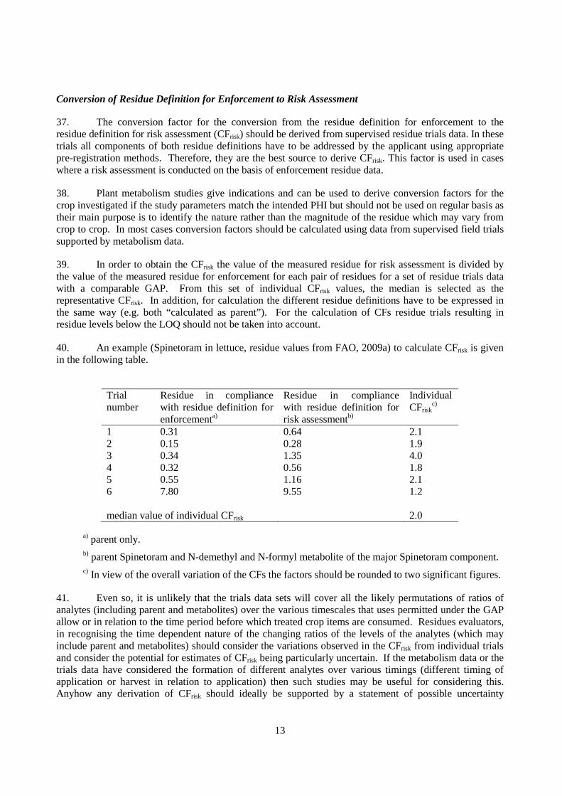
40. An example (Spinetoram in lettuce, residue values from FAO, 2009a) to calculate CFrisk is given in the following table.

Trial number

Residue in compliance with residue definition for enforcementa)

Residue in compliance with residue definition for risk assessmentb)

Individual CFrisk

c)

1 0.31 0.64 2.1 2 0.15 0.28 1.9 3 0.34 1.35 4.0 4 0.32 0.56 1.8 5 0.55 1.16 2.1 6 7.80 9.55 1.2 median value of individual CFrisk 2.0

a) parent only. b) parent Spinetoram and N-demethyl and N-formyl metabolite of the major Spinetoram component. c) In view of the overall variation of the CFs the factors should be rounded to two significant figures.

41. Even so, it is unlikely that the trials data sets will cover all the likely permutations of ratios of analytes (including parent and metabolites) over the various timescales that uses permitted under the GAP allow or in relation to the time period before which treated crop items are consumed. Residues evaluators, in recognising the time dependent nature of the changing ratios of the levels of the analytes (which may include parent and metabolites) should consider the variations observed in the CFrisk from individual trials and consider the potential for estimates of CFrisk being particularly uncertain. If the metabolism data or the trials data have considered the formation of different analytes over various timings (different timing of application or harvest in relation to application) then such studies may be useful for considering this. Anyhow any derivation of CFrisk should ideally be supported by a statement of possible uncertainty

14

associated with a derived value and should ensure that the scope of relevance of using the conversion factor is clear (the crop or crops to which the CFrisk factor would be applicable).

42. For illustration the following example is provided for spirotetramat (European Food Safety Authority 2013). For this active substance, an overall CF for risk assessment of two has been proposed in the EFSA conclusion considering the CF derived for a total of 19 crops at various PHIs. Note: This example shows dependency on the PHI. However PHI is normally only the minimum waiting period of a GAP, and CF may significantly increase for periods beyond PHI.

CF for spirotetramat at different PHIs Total

samples PHI (days) 0- 0+ 3 7 14 21 28 Citrus 1.7 1.2 1.4 1.6 1.7 1.8 87 Pome fruit 1.7 1.2 1.4 1.6 1.7 1.9 124 Peach 1.7 1.3 1.5 1.7 2.1 2.4 68 Plum 1.6 1.3 1.4 1.8 2.2 2.7 60 Cherry 1.7 1.3 1.3 1.6 1.8 2.1 58 Grape 1.5 1.4 1.2 1.4 1.6 1.9 40 Strawberry (Out) 1.8 1.4 1.3 1.4 1.7 39 Strawberry (In) 1.3 1.1 1.2 1.2 1.3 36 Onion 1.7 1.6 1.6 1.6 1.6 1.6 72 Tomato 1.4 1.3 1.4 1.5 1.9 50 Pepper 1.2 1.2 1.2 1.2 80 Cucumber 2.4 2.1 2.3 2.4 58 Melon 2.4 2.3 2.4 2.4 65 Brassica flowering 2.0 1.8 2.0 2.4 2.2 1.6 65

Brassica head 2.1 1.7 1.9 1.8 1.8 1.8 114 Brassica leafy 1.4 1.2 1.3 1.5 1.5 1.7 42 Kohlrabi 1.2 1.2 1.2 1.2 1.2 1.3 23 Lettuce (Out) 1.7 1.2 1.5 1.7 2.5 32 Lettuce (In) 1.4 1.1 1.1 1.3 1.8 78 Bean (with pods) 2.1 1.7 1.9 1.8 1.8 40 Hops 1.9 1.7 1.7 20 Overall mean CF 1.7 1.4 1.5 1.6 1.7 1.8 2.2 1251

Explanations

- Residue definition for enforcement: Sum of spirotetramat and spirotetramat-enol expressed as spirotetramat.

- Residue definition for risk assessment: Sum of spirotetramat, spirotetramat-enol, spirotetramat-ketohydroxy, spirotetramat-monohydroxy and spirotetramat-enol-Glc, expressed as spirotetramat.

- CF at requested PHI are greyed.

15

43. The above described approach can also be used for feed commodities when calculating dietary burden, if the residue definition for monitoring differs from the residue definition that should be used for exposure of animals to residues in the feed commodities.

Conversion Factor for Edible Parts

44. The conversion factor for the conversion from whole product to the edible part should be derived from supervised residue trials data (based on the residue definition for enforcement) and is in principle a processing factor. For this reason it should be abbreviated as a processing factor (PFedible). In order to obtain the PFedible the value of the measured residues in the edible commodity is divided by the value of measured residues in the whole commodity for each pair of residues for a set of residue trials data with a comparable GAP. From this set of individual PFedible values, the median is selected as the representative PFedible.

5. Formulations

45. Most types of formulations can be divided into two groups – those which are diluted with water prior to application and those which are applied intact. Emulsifiable concentrates (EC) and wettable powders (WP) are examples of the first type whereas granules (GR) and dusts (DP) are the most common examples of the latter. Some special types of formulations are described in paragraphs 52-53. A description of the various types of formulations including coding is given in the Manual of the Joint Meeting on Pesticide Specifications (JMPS) (FAO, 2010) [see also Table 2].

Formulations Diluted in Water

46. The most common formulation types which are diluted in water prior to application include EC, WP, water dispersible granules (WG), suspension concentrates (SC) (also called flowable concentrates), and soluble concentrates (SL). Residue data may be translated among these formulation types for applications that are made to seeds, prior to crop emergence (i.e., pre-plant, at-plant, and pre-emergence applications) or just after crop emergence. Data may also be translated among these formulation types for applications directed to the soil, such as row middle or post-directed applications (as opposed to foliar treatments).

47. In a recent publication by Maclachlan and Hamilton (2010) it was shown by evaluation of side-by- side trials with the same application rate and similar spray volumes that WP, EC, CS (capsule suspension) and SC formulations do not show a significant difference in day-zero residues after foliar treatment (JMPR data from 2000 to 2004). The evaluation includes trials with PHIs of less than seven days. For mid-season and late-season foliar applications of formulations diluted in water, those formulations not containing oils or organic solvents (e.g., WG, SC) are considered equivalent and those containing oils or organic solvents (e.g., EC, OD) are also considered equivalent. Some authorities may require bridging data between the two formulation types (to demonstrate similarity of residue levels) where a complete data set exists for one type.

48. The publication by Maclachlan and Hamilton (2010) was available after the publication of OECD Test Guideline No. 509; for this reason the above paragraph appears in contradiction of paragraph 27 of the Test Guideline. Consequently it is recommended that paragraph 27 of the OECD TG 509 be further revised accordingly.

Water Soluble Bags

49. Placing a formulation (typically WP) in a water soluble bag does not require additional residue data provided adequate data are available for the unbagged product and the formulation chemistry data

16

provided show acceptable dissolution of the water soluble bag will be expected under practical conditions of use.

Formulations Applied Intact

50. Granular formulations applied intact will generally require a complete data set regardless of what data are already available for other formulation types. This is based on several observed cases of residue uptake being quite different for granules versus other types of formulations of the same active ingredient.

Formulations Designed for Seed Treatments

51. Some formulations are often designed specifically for seed treatment use such as DS powder for dry seed treatment use and ES emulsion for seed treatment. Residue data for seed treatment uses may be translated between such formulations. Nevertheless, it may be necessary to consider the chemical loading data for assurance on translation of the residue data for these formulations.

Controlled Release Formulations

52. Controlled release formulations (e.g., certain microencapsulated products) normally require a complete data set tailored to that particular use. Since these formulations are designed to control the release rate of the active ingredient, different residues are possible compared to other formulation types.

Formulations that Contain Active Substances as Nanomaterials

53. In general it is expected that if active substances were to be formulated as nanomaterial they would have different properties compared to normal sized material. At present no definitive statement can be made as to whether or not current data requirements are sufficient to carry out risk assessments for nanopesticides. For the time being a complete data set is needed for plant protection products containing nanomaterials in order to compare residue behaviour with conventional products.

6. Geographical Distribution of Residue Trials

54. In response to one of the recommendations of the workshop in York in 1999 (OECD 2003) on "Developing Minimum Data Requirements for Estimating MRLs and Import Tolerances", the OECD Working Group on Pesticides and the FAO Pesticide Management Group invited a small group of residue experts from OECD and FAO Member countries to develop the concept of a global zoning scheme to define areas in the world where pesticide trials data could be considered comparable, and therefore where such trials could be used within each zone for MRL-setting purposes, irrespective of national boundaries (OECD 2003).

55. On the basis of the underlying assumption that residues depend on climatic conditions and that it might be possible to develop a climate-based residue zoning scheme, an extensive database of residue trials data from the FAO/WHO Joint Meeting on Pesticide Residues (JMPR) Residue Evaluations was collected and then analysed by an independent statistician. The outcome from this analysis was that:

• There was sufficient information to indicate that a residue zoning scheme, based on climatic differences alone, could not be proposed because of the high variation in residues reported from comparable trials even within the same climatic zone.

• Pre-harvest climatic conditions were not major factors influencing residue variability in comparable residue trials.

17

• Most of the residue variability at harvest reported from comparable trials was associated with variability in residues at ’zero-days’ (assumed to be largely unaffected by pre-harvest climatic conditions).

• Many of the factors possibly contributing to residue variability in comparable residue trials have already been recognised, to a greater or lesser extent, in the MRL assessment procedures established at the national, regional and international level, with residue trials being designed to reflect the range of production systems and climate situations that might be expected during the commercial use of the product.

56. The main point addressed in the OECD report was that national boundaries are not a barrier to acceptance of supervised field trials from other regions. This point was used by JMPR and some national/regional authorities at the time of publication. Unfortunately, the recommendations of this report were not considered further and the results were not much used by national or regional evaluation or legislation.

57. The results of the above project were used to support the proposal that for comprehensive OECD submissions (see paragraphs 68 to 79) the number of residue trials can be reduced by 40%. The EU now allows to a certain extent to replace the number of trials necessary by trials from outside Europe, provided that they correspond to the critical European GAP (within the ± 25% rule) and that the production conditions (e.g. cultural practices) are comparable (European Commission 2013). Canada and the United States allow substitution of some US/Canadian trials by trials from outside the US/Canada on a case-by-case basis provided the crop cultural practices, climatic conditions, and use pattern are substantially similar to those of the subject US/Canada region(s).

58. The analysis of the above mentioned project also forms the basis of the recommendations in OECD Test Guideline 509 (OECD, 2009) to generally accept data from only one season, rather than requiring data sets to be conducted typically over two or more seasons, provided that crop field trials are located in a wide range of crop production areas such that a variety of climatic conditions is taken into account. Despite this, where there is evidence of particular seasonal variations in data, it is reasonable to require more data.

59. In an earlier discussion in the OECD Residue Chemistry Expert Group it was recommended to confirm the results by evaluating five different major crops (e.g., grain, leafy vegetable, fruiting crop, root crop, oilseed) with realistic non-zero PHI residues data (difficult to achieve meaningful data for root crops) from different OECD countries/regions laying emphasis not only on foliar applications but also taking other applications techniques into account. Results from other application techniques should complete that project. Different types of pesticides (insecticides, herbicides, etc.) with both systemic and non-systemic properties should be represented.

New Data Evaluation

60. In an example of a global residue program provided by Dow AgroSciences (C. Tiu, 2011, 2012) quantifiable residue data were generated at critical GAP for foliar application of the active substance sulfoxaflor over a 2-3 years period in four different regions of the world (Europe, North America, Australia, New Zealand and Brazil) for 39 crops, to support OECD global joint review, Codex-MRLs and multiple national registration processes. Residues data were analysed for commodities representing leafy vegetables, Brassica vegetables, fruiting vegetables, fruit trees, oilseeds and cereal grains. Root crops were not considered due to very low or no detectable residues. Residue datasets for this active substance showed the best goodness of fit for log normal distribution (68%), followed by normal distribution (21%) and unknown distributions (11%). Results for all crops showed that data analysed by ANOVA is

18

statistically similar across the different regions/zones (p > 0.05). The results of the Turkey test (one possible ANOVA post-hoc analysis) showed no significant difference between the means of the residue data by regions. Variability between trials within a zone was higher than the variability between regions (2-20x). It represented in average 78% versus 12% average contribution from zone. The remaining 10% variation is assumed as a residual effect proceeding from duplicate samples, analytical variability, etc.

61. In order to make further progress in the geographical distribution of residue trials, the above conclusions were validated by US-EPA in the light of recent OECD joint submissions and US-Canadian residue database used for NAFTA MRL harmonization. 79 different crops (e.g., cereal grains, several types of vegetables, different fruit commodities, oilseed crops, root crops) were tested for 73 pesticides (insecticides, fungicides, herbicides) in two to 23 OECD countries/regions, covering six geographical regions and four climatic zones. Statistical analysis using linear mixed effects model analysis confirmed greater variability of data within than between regions/climates. This is confirming former findings (OECD, 2003) and provides the evidence required to fill in the gaps pointed out by previous validations.

Conclusion and Recommendation for Geographical Distribution of Residue Trials

62. Current evidence suggests that residue data generated at similar GAP in different geographical regions/climatic zones may be used as a consolidated global dataset for MRL setting. Like for application of the proportionality principle, the associated uncertainty is interpreted within the ±25% deviation of supervised field trials. The distribution of the trials should be in at least two different regions or 50% of the number of regions pursuing registration, in order to provide the minimum number of trials required and a representative distribution for comprehensive global programs. At a later stage the number of trials as described below and given in Table 3 should be carefully reconsidered in light of future regulatory requirements in different countries.

63. The overall aim is to define for a given GAP that is used in more than one Country or region – a Global GAP (not necessarily meaning that it is used all over the world) – a number of acceptable trials and how to distribute them in more than two regions in order to be accepted as a common data set for this Global GAP.

Due to the limited amount of information on possible zoning of residue trials, a recommendation that will be used from the Report of the OECD/FAO Zoning Project is the acceptance of trials from other regions.

7. Number of Trials

National/Regional Approach to Number of Trials

64. National/regional requirements concerning number of residue trials per crop remain in place. To a certain extent the total number of trials required by a regulatory authority may include trials conducted in another region provided that these trials correspond to the critical GAP and the production conditions, i.e. with comparable cultural practices. Before combining residue data, the protocols should be studied carefully as to whether they met these criteria.

Codex Approach to Number of Trials

65. JMPR performs the evaluation of the submitted information and estimates maximum residue levels if the database is considered sufficient, regardless of whether it represents worldwide use or is limited to a region. The number of trials (generally minimum 6-10) and samples is dependent on the variability of use conditions, the consequent variation of the residue data, and the importance of the commodity in terms of production, trade and dietary consumption.

19

Recommendations for Comprehensive Data Submissions

66. In the case of a comprehensive submission to all OECD countries where the desired GAP is uniform, a 40% reduction in the total number of trials is feasible, compared to the total number of trials determined by summation of individual country requirements. The residue trials chosen are those conducted independently. The assumption is that the number of trials specified in each crop production region reflects the economic (acreage) importance and/or dietary significance of the representative crop commodity(ies) within that production region.

67. The reduction in the total number of trials within any OECD country or crop production region is compensated for by the total number of crop field trials making up the comprehensive submission data set and the wider geographic distribution of these data. With this 40% reduction, regulatory authorities may receive fewer crop field trials conducted in their specific country or region; however they will actually receive a greater number of trials in total with a more comprehensive geographical distribution. There are precedents in OECD countries and regions for this approach.

68. To qualify for this comprehensive submission approach, all crop field trials as requested by national/regional authorities should meet the following criteria:

• Field trials are conducted according to the cGAP (within ± 25% of the nominal application rate, number of applications or PHI). For comprehensive submission at least 50% of the trials should be conducted at or above (within 25%) the cGAP. For this purpose, trials whose intended application rates match the cGAP but actual rates fall down to 10% below the cGAP (e.g., due to the normal variability in preparing spray solutions) are considered acceptable. If more than 50% of the trials were conducted at actual rates below that of the cGAP (but within 25%), the proportionality approach can be used by the scaling of the entire dataset to the nominal dose.

• Although it is possible to use results from residue trials that are not conducted according to cGAP but calculated according to the proportionality principle, the combining of both concepts – reduction of number of trials and proportionality – should be used with caution due to the lack of experience in both concepts.

• Some authorities request up to 50% of the trials to be decline studies;

• The trials should cover a range of representative crop production practices for each crop including those likely to lead to the highest residues (e.g., irrigated vs. non-irrigated, trellis vs. nontrellis production, autumn-planted vs. spring-planted, etc.).

• Trials that are substituted by trials from another country should not be used for across the board reduction. For example, a trial can be considered only one time and cannot count toward the total number of trials both in the country where conducted and a second time in another country or region where it would be substituted for a local trial.

69. The minimum total number of trials for any crop in a comprehensive submission is eight. In addition, the total number of trials to be conducted must not be less than the requirement for any given individual region. For example, upon calculation of the 40% reduction, some crops such as dried lima beans have fewer total trials [14] than required in one region [16 in the EU]. Therefore, at least 16 trials are needed for dried lima beans in a comprehensive submission.

70. Any reduction in the number of crop field trials should be distributed proportionally among the crop production regions as shown in the example for a 40% reduction for barley below. Table 3 gives the

20

trial numbers for crops grown throughout OECD countries. If the number of required trials changes in any given region, Table 3 should be adjusted accordingly.

71. In the example given below the total number of trials is 31, which represents a 40% reduction compared to 52.

Country or Region NAFTA EU JP AUS NZ Total

Number without reduction 21 16 3 8 4 52

Number with 40% reduction 12 10 2 5 2 31

72. This means that for a global submission, instead of a total of 52 trials a total of 31 trials is sufficient. These trials should meet the requirements defined in paragraph 69. The total of 31 trials should be distributed across the regions as indicated in the table.

73. In no case the number of trials in a given crop production region may be reduced below two. Thus, the 40% reduction does not apply to a crop for which the required number of trials is two. In such a case the number of trials is two before and after reduction.

74. It is important to keep in mind that this comprehensive strategy would only apply to an OECD wide submission. If, for example, the MRL submission is originally submitted to the US and Canada, the crop field trial guidelines, with respect to the number of trials, for those countries should be followed. Subsequently, if MRLs in additional OECD countries are pursued, the regulatory authorities in the additional countries should be consulted to determine what residue data are required. For example, following establishment of an MRL in the US and Canada, if an MRL for the same use is pursued in the EU, the applicant may consult with EU regulatory authorities about the possibility of using residue data from the US/Canadian data submission and performing fewer crop field trials in the EU.

75. The table of trial numbers in the Table 3 addresses only outdoor crop field trials and not greenhouse (glasshouse) or post-harvest treatments. For a comprehensive submission to OECD countries, concerning greenhouse uses, a minimum of eight greenhouse trials is needed, but not less than the requirement for any given individual region. For such greenhouse trials, geographic distribution typically is not an issue; however for active ingredients which are susceptible to photodegradation, consideration should be given to locations at different latitudes and winter/summer periods.

76. The number of post-harvest trials on a commodity should be at least four,but no less than the requirement for any given individual region, taking into consideration the application techniques, storage facilities, and packaging materials used. Changes in the mentioned conditions may require additional trials.

77. As stated in paragraph 62 further considerations are useful in the light of experience gained in future.

8. Results from Residue Trials to be used in MRL Estimations

78. In principle all data from residue trials conducted according to cGAP and considered valid should be taken into account for MRL setting. Nevertheless a few questions often arise and some of the main ones are discussed in the following paragraphs.

21

Handling of Outliers

79. Residue values above the majority of the data population are always suspicious and therefore are often characterised as outliers. Nevertheless, before disregarding a result as an outlier the study should be carefully examined to see if there is adequate information and/or experimental evidence to justify its exclusion. The exclusion of an apparent outlier must be justified by agricultural practice or other evidence deriving from the experimental set up or analytical conditions. Statistical results, in and of themselves, are generally not sufficient to exclude data from the MRL-setting process.

Multiple Component Residues

80. Where the active substance and at least one metabolite, degradation or reaction product is included in the residue definition two cases have to be considered: either the components are converted to a single component or analyte by the analytical method or the components are determined separately.

81. In the first case the total residue is measured as a single compound and expressed as the parent compound or in some circumstances as a metabolite or degradation product. As in any other case the LOQ is usually determined by the lowest validated level of analyte. The MRL estimate is based on the measured residues for the total residue.

82. In the second case residue components are determined separately by the method of analysis. The concentrations of measurable residues are adjusted for molecular weight and summed, and their sum (normally parent equivalent residues) is used for estimating the maximum residue level. Nevertheless, some guidance is necessary if the residues for some or all the components are at or below the LOQ. This is explained using the following example.

General Example

83. Note: example based on the FAO Manual for bentazone with fictive values. The residue definition is given as "parent, metabolite 1 and metabolite 2 expressed as parent". The LOQ of the method of analysis for the single components of the residue definition is 0.02 mg/kg. The different situations are described in the following table.

Example Maximum levels (mg/kg) detected for components

(supervised residue trials) Recommended total

residue (mg/kg) Parent metabolite 1 metabolite 2 (expressed as Parent)

(a) <0.02 <0.02 <0.02 <0.06 (b) 0.04 <0.02 <0.02 0.08 (c) 0.04 0.03 <0.02 0.09 (d) <0.02 0.04 0.05 0.11

84. This recommendation in the table is based on the assumption that it might be possible to improve the method of analysis to achieve for example a LOQ of 0.01 mg/kg. Re-examination of the results may then give residues only slightly below 0.02 mg/kg for each of the single compounds and 0.06 mg/kg for the sum. The recommended total residues from the table should be used in MRL estimations. Referring to example (a) it is important to maintain the "<", since the individual components were all <LOQ and the number of censored data is relevant for the calculation.

22

85. A problem arising from this recommendation is discussed as follows: a MRL of 0.06 mg/kg would allow any residue component to be present at 0.06 mg/kg, or all of the three at 0.02 mg/kg, without exceeding the MRL. Consequently, individual residue components could be three times those which should arise from GAP-compliant use of the compound but would be within the MRL.

86. It is recommended that decisions on the levels of MRLs at or about the practical limit of quantification should particularly take into account the following factors:

• Toxicity of the active ingredient as indicated by the ADI or the ARfD. Normally, low ADIs or ARfDs should be accompanied by relatively low limits of quantification. The lower limit used may also have implications for risk assessment calculations.

• In principle, the lower the residue arising from GAP, the lower the limit of quantification should be.

• The limit used in the supervised residue trials is also a consideration which should be taken into account. A LOQ may not normally be established at a level lower than that used in the generation of the data. However, should other factors be considered determinant, regeneration of the data using a more appropriate lower limit may be required.

• As analyses at lower levels will influence enforcement costs, the expenditure/benefit evaluation will influence the final decision on the appropriate limit of quantification.

• Evidence from metabolism studies, chromatograms and other information on the relative concentrations of the various residue components.

Independent Supervised Residue Trials

87. As a principle only one result from each residue trial that is within cGAP should be used for the estimation of MRLs. In addition, selected results should only be used from independent supervised residue trials. When considering independence of supervised residue trials OECD recommends that each of the following factors should be considered separately:

• Geographical location and site – Trials at different geographic locations are considered independent.

• Dates of planting (annual crops) and treatments – Trials involving significantly different planting dates or treatment dates (> 30 days apart) are considered independent.

88. Additional factors may influence the independence and may be taken into consideration on a case by case basis:

• Crop varieties – Some varieties may be sufficiently different (e.g. different size at maturity, rough vs. smooth surface, different amount of foliage) to influence the residue and could be considered independent.

• Formulations – Trials conducted with different formulations should not be considered independent. Exceptions can be derived from chapter 5, i.e. granular formulations, controlled release formulations and formulations based on nanomaterials that need a separate dataset. In this case a statistical test is required to see whether residues from these formulations differ from those with water diluted formulations. If they differ, they can be considered independent.

23

• Application rates and spray concentrations – Trials at different application rates and spray concentrations should not be considered independent.

• Treatment operations – Trials using the same spray operation are not considered independent.

• Application equipment – Trials using different equipment are not considered independent.

• Addition of adjuvants – A trial with the addition of an adjuvant should not be considered independent. If an adjuvant will be routinely recommended or included in the marketed formulation, then the trials should use the adjuvant. If the use pattern includes mid-season to late-season foliar application, consideration should be given to including appropriate adjuvants in a portion of the trials.

89. Only one field trial would normally be selected per trial site if multiple plots/trials are conducted in parallel, unless one or more of the conditions outlined above apply, e.g., significantly different varieties in the replicate plots. For trials at the same location there should be convincing evidence that additional trials are providing further independent information on the influence of the range of farming practices on residue levels.

90. For trials being considered independent the measured residue is used in MRL estimates. For those trials being considered as not independent the measured residues should be treated as being replicates (see below).

Replicates

91. Various scenarios may apply when several residue values are described as "replicates" such as when there are:

• Replicate analysis samples from one laboratory sample (duplicate analysis).

• Replicate laboratory samples obtained with sub-division from one field sample.

• Replicate field samples analysed separately (each sample is taken randomly from a plot which was treated as a whole).

• Replicate plots or sub or split-plot field samples are analysed separately (the whole trial is subject to the same spraying treatment, but it is divided into two or more areas that are sampled separately).

• Replicate trial samples are analysed separately (trials from the same site that are not independent may be considered as replicate trials).

92. In all cases the type of replicate should be specified when assessing the data. The average or mean value of replicates should be used as the representative value for that field trial in exactly the same fashion that is done for analytical replicates of the same composite sample. From a statistical point of view, the mean or average residue value of replicate samples provides the basis for setting MRLs targeted at the p95 of the underlying distribution. However, there may be situations where single valid results from replicate samples may exceed the MRL estimated from the use of average or mean values. In such situations and in view of consumer safety, consideration may be given by some regulatory authorities to the use of these single values as the HR in dietary risk assessment.

24

93. Also JMPR has checked this approach in 2010 and concluded to use the average of replicate field samples in establishing the data set for statistical calculation of maximum residue level estimates. However, JMPR also noted that the interpretation of the estimate must take into account individual replicate values contributing to the data set that exceed the estimate. For such situations JMPR will still use the HR, to avoid missing the HR value for dietary risk assessment. JMPR continues to select the highest residue value for MRL derivation in case of two or more trials that are not considered independent.

Residues at Harvest

94. Normally, the residue at the PHI specified in the cGAP should be used for the MRL estimation. Nevertheless, the residue trial data should be assessed carefully and higher residues at longer PHIs should be used instead of the residue at the cGAP as this safety interval is defined as the shortest possible meaning that harvest at later stages may take place. In case of replicates take first a decision on handling as recommended (see paragraphs 92-94).

95. In some cases the time of application is well defined by the growth stage (BBCH; a decimal code system, which is divided into principal and secondary growth stages1). In this case setting of a PHI is not necessary. The selection of the results from residue trials then depends on the use of the plant protection product at the correct growth stage and the normal harvest of the product.

9. MRL Estimations

Considerations for MRL-setting based on specific Use Patterns

96. The post-harvest use of a persistent, non-volatile active substance in stored products will lead to residues that can be calculated on the basis of the amount used to treat the stored commodity for short waiting periods. The MRL should not be set at a higher level than the application rate equivalent, but higher maximum residue levels may need to be considered on a case by case basis to account for inhomogeneous distribution of the pesticide during application or sampling difficulties (especially bulk commodities). Any variation in residues depends on the precision of the application especially concerning the deposition of the active substance on the surface of the treated commodity. Environmental and commodity related factors (like metabolism) will only have limited influence. Residue trials are necessary to reflect storage locations with variable conditions regarding temperature, humidity, aeration, etc. Once the relationship between application rate and residue level has been shown, additional trials with other application rates are not necessary. This relationship is based on special environmental and commodity factors independent from the conditions of the proportionality principle.

97. The OECD MRL calculator may not be a suitable tool to propose MRL for post-harvest application. In such a case, the estimate calculated as "CF X3 mean" should normally be disregarded and the MRL proposal based on the estimates calculated as "Mean + 4 SD" or "Highest residue" and considering the nominal application rate.

98. For seed treatments a situation could be imagined, where the worst-case MRL based on the ai-content in the seed, the known seed density and the known yield of the commodity would be estimated being below the LOQ or below an already existing MRL. In that case and assuming that possibly formed metabolites are adequately covered, a waiver for additional residue trials with a new application rate might be acceptable. Seed treatments for such a consideration exclude potato seed treatments: This is related to the different growing situations. In case of potatoes distribution into the daughter tubers has been taken into account. Such situations will occur, for example, in seed treatments of cereals or carrots. 1 A description in German, English, French, or Spanish can be downloaded from: http://www.jki.bund.de/en/startseite/veroeffentlichungen/bbch-codes.html

25

Selecting of Data for Using the OECD Calculator in MRL Estimations

99. A statistical calculator has been developed by OECD for determination of MRLs from valid field residue data. The calculation process is based on "mean + 4SD" methodology. A White Paper and related user guide are available as additional resources (OECD 2011). The OECD Calculator itself is provided as an excel spreadsheet either for single data set or for multiple data sets.

100. For the OECD calculator method of MRL calculation, it has been determined that the mean or average residue value, when replicate sample data have been generated per field site, should be used in the calculation process (see paragraph 93).

101. Several examples of criteria, used in selecting data to be considered in the MRL calculation, require expert judgement and consultation with national/regional authorities:

• Use of censored data (i.e. <LOQ). The default inputs to the calculator for these values are the respective LOQ values with an asterisk designation for censored data. The calculator uses a censoring factor to correct for residues reported at the LOQ that were less than the LOQ. Care must be taken when large parts of the data set consist of censored data. In such cases the calculator indicates less reliability of results.

• Proposing MRLs lower than 0.01 mg/kg. The calculator’s lowest accepted residue value is 0.001 mg/kg. The calculator will work with values below 0.01 mg/kg and will display statistical values below 0.01 mg/kg including unrounded MRL. The proposed MRL will be always the lowest MRL class of 0.01 mg/kg. On the basis of these data it is possible to round the results to an appropriate MRL class below 0.01 mg/kg if guaranteed. Nevertheless, MRLs below 0.01 mg/kg are an exception for the moment and routine MRL setting below this value should be discussed in the light of future developments in analytical methods.

• Small datasets: If the dataset consists of less than three values the message "MRL calculation not possible. [Too small dataset]" is displayed at the bottom of the spreadsheet. The choice of three values was made based on the minimal requirement common among OECD countries. With a single residue value, it is impossible to compute an estimator for the standard deviation of the dataset, which is needed in the calculation procedure. If the dataset consists of 3-7 residue values, the message "High uncertainty of MRL estimate, [Small dataset]" is displayed to remind the user of the considerable level of uncertainty surrounding the calculation of any statistical quantity for such small datasets. [For information: NAFTA countries on rare occasions for a very minor crop must make an MRL estimate from 2 independent field trials (n = 2). Various options were considered, and it was found that 5 X Mean provides the best estimate for outdoor trials and 3 X Mean provides the best estimate for greenhouse trials. This is based on simulations.]

• Data selection from dependent residue trials (those that are not assessed as independent from one another) – In case of dependent data the average of the residue values from the dependent trials should be used in the OECD Calculator if provided these trials are statistically not different. Otherwise the highest measured residue is used.

• Combining of datasets for the same crop commodity treated at closely related GAP (i.e., cGAP within maximum 25% deviation in one of the key parameters) – The term closely related GAP will exclude data sets that differ, for example, in application type (broadcast foliar versus ground application) or in kind of production (indoor versus outdoor production). Closely related GAPs are for example those where high volume and low volume spray is used. In this case, it should be determined if the residues are comparable, that is, if they belong to the same residue population

26

(see paragraph 15), or if they should be handled separately. If the data sets are not comparable, the MRL should be calculated for each dataset separately and the MRL from the highest residue population should be used.

• Combining/separating datasets for the same ai/crop/GAP combination generated with different LOQs and containing some censored data – Combine the data sets.

• Combining/separating datasets for the same ai/crop/GAP combination generated with different LOQs and all measured residues are below the LOQ – Where there are two or more data sets consisting of residue data with different LOQ levels, the set with the lowest LOQ should be preferred for MRL setting (given it is sufficient as such) as it usually reflects state-of-the-art analytical methods.

• Combining datasets from different regions (e.g. NAFTA and EU) for the same crop commodity treated at the same GAP (see paragraph 15) – Northern and southern residue region in Europe are considered in the first step as different regions. It should be determined if the residues are comparable, or if they should be handled separately. If the data sets are not comparable, the MRL should be calculated for each dataset separately and the MRL from the highest residue population should be used.

• Combining of datasets from different crop commodities for the same crop group treated at the same GAP. – Values should not be combined for morphologically different crops.

• Combining data sets from the same species differing in size – Sometimes authorities differentiate between small size and large size varieties. For example Codex will in future require trials on sweet pepper; and one cultivar of chili pepper or one cultivar of large variety of eggplant and one cultivar of small variety eggplant for extrapolation to the entire crop group. Though requiring trials on varieties of different size, the data will normally be combined in one population (with probably high variability) since the same MRL is applicable for all varieties and statistical tools are normally not applicable for such very small data sets.

102. The OECD calculator is useful to determine whether an MRL estimate is appropriate on the basis of a particular data set. However, a reviewer is aware of other factors which may influence the values at which MRLs are set. It is therefore important to note that although the calculator is a beneficial tool, the decision about the most appropriate MRL should be made by the reviewer, who is in possession of all the relevant information.

10. References

Australian Pesticides and Veterinary Medicines Authority 2000. Residue Guideline No. 24. http://www.apvma.gov.au/publications/guidelines/rgl_24.php#top

Codex Alimentarius Commission, 1993. Codex Alimentarius, Volume 2 Pesticide Residues in Food.

2nd Ed. Section 2 Codex Classification of Food and Animal Feeds. Food Joint FAO/WHO Food Standards Programme, Rome, 1993.

Codex Alimentarius Commission, 2004. Report of the Thirty-Sixth Session of the Codex Committee on

Pesticide Residues. Alinorm 04/27/24, para 248 – 258. New Delhi, India, 19 - 24 April 2004. Codex Alimentarius Commission, 2004. Twenty-seventh Session. Report Alinorm 04/27/41, Appendix VI.

Centre International de Conférences de Genève, Geneva, Switzerland, 28 June – 3 July 2004.

27

Codex Alimentarius Commission, 2006. Report of the Thirty-Eighth Session of the Codex Committee on

Pesticide Residues. Alinorm 06/29/24, para 160 – 171.Fortaleza, Brazil, 3 - 8 April 2006. Codex Alimentarius Commission, 2006. Twenty-ninth Session. Report Alinorm 06/29/41, Appendix VIII.

Centre International de Conférences de Genève, Geneva, Switzerland, 3 – 7 July 2006. Codex Alimentarius Commission, 2007. Report of the Thirty-Ninth Session of the Codex Committee on

Pesticide Residues. Alinorm 07/30/24, para 142 – 152 and CX/PR 07/39/4, Beijing, China, 7-12 May 2007.

Codex Alimentarius Commission, 2008. Report of the Fortieth Session of the Codex Committee on

Pesticide Residues. Alinorm 08/31/24, para 107 – 115 and CX/PR 08/40/4, Hangzhou, China, 14-19 April 2008.

Codex Alimentarius Commission, 2009. Report of the Forty-First Session of the Codex Committee on

Pesticide Residues. Alinorm 09/32/24, para 131 – 155, CX/PR 09/41/4 and CX/PR 09/41/4 Add. 2, Beijing, China, 20 - 25 April 2009.

Codex Alimentarius Commission, 2010. Report of the Forty-Second Session of the Codex Committee on

Pesticide Residues. ALINORM 10/33/24, para 73, 86 – 118, Xian, China, 19 - 24 April 2010. Codex Alimentarius Commission, 2011. Report of the 43rd Session of the Codex Committee on Pesticide

Residues. REP11/PR, para 24, 82 – 86, Beijing, China, 4 - 9 April 2011. Codex Alimentarius Commission, 2012. Report of the Forty-fourth Session of the Codex Committee on

Pesticide Residues. REP12/PR, Shanghai, China, 23 - 28 April 2012. Codex Alimentarius Commission, 2012. Report of the Thirty-fifth Session of the Codex Alimentarius

Commission. REP12/CAC, Rome, Italy, 2 - 7 July 2012. Codex Alimentarius Commission, 2013. Report of the 45th Session of the Codex Committee on Pesticide

Residues. REP13/PR, Beijing, China, 6 - 11 May 2013. Environmental Protection Agency 1996. Residue Chemistry Test Guidelines – OPPTS 860.1000 Residue

Chemistry Test Guidelines and 860.1500 Crop Field Trials. http://www.epa.gov/opptsfrs/publications/OPPTS_Harmonized/860_Residue_Chemistry_Test_Gui

delines/Series/860-1000.pdf European Commission, 2008. Guidance Document, Guidelines on comparability, extrapolation, group

tolerances and data requirements for setting MRLs. SANCO 7525/VI/95 – rev. 9, to be adopted in December 2010.

European Commission, 2013. Commission Regulation (EU) 283/2013 of 1 March 2013 setting out the data

requirements for active substances, in accordance with Regulation (EC) No 1107/2009 of the European Parliament and of the Council concerning the placing of plant protection products on the market. OJ L 93, 03.04.2013, p. 1-84.

European Food Safety Authority, 2013. Conclusion on the peer review of the pesticide risk assessment of

the active substance spirotetramat. EFSA Journal 2013;11(6):3243, 90 pp.

28

FAO, 2009a. Pesticide residues in food—2008. Evaluations Part I – Residues. FAO Plant Production and Protection Paper, 194, 2009.

FAO, 2009b. Submission and evaluation of pesticide residues data for the estimation of maximum residue

levels in food and feed (FAO Manual, 2nd Edition). FAO Plant Production and Protection Paper, 197, 2009.

FAO 2010. Manual on development and use of FAO and WHO specifications for pesticides. Prepared by

the FAO/WHO Joint Meeting on Pesticide Specifications (JMPS) November 2010 – Second Revision of the First Edition. FAO, WHO, Rome 2010.

FAO, 2011a. Pesticide residues in food—2010. Report of the Joint Meeting of the FAO Panel of Experts

on Pesticide Residues in Food and the Environment and the WHO Core Assessment Group. FAO Plant Production and Protection Paper, 200, 2011.

FAO, 2011b. Pesticide residues in food—2011. Report of the Joint Meeting of the FAO Panel of Experts

on Pesticide Residues in Food and the Environment and the WHO Core Assessment Group. FAO Plant Production and Protection Paper, 211, 2011.

FAO, 2013: Pesticide residues in food—2012. Report of the Joint Meeting of the FAO Panel of Experts on

Pesticide Residues in Food and the Environment and the WHO Core Assessment Group. FAO Plant Production and Protection Paper, 215, 2013.

FAO 2014: Pesticide residues in food—2013. Report of the Joint Meeting of the FAO Panel of Experts on

Pesticide Residues in Food and the Environment and the WHO Core Assessment Group. FAO Plant Production and Protection Paper, 219, 2014.

FAO 2015: Pesticide residues in food—2014. Report of the Joint Meeting of the FAO Panel of Experts on

Pesticide Residues in Food and the Environment and the WHO Core Assessment Group. FAO Plant Production and Protection Paper, 221, 2015.

MacLachlan, D. J. and Hamilton, D., 2010. A new tool for the evaluation of crop residue trial data (day-

zero-plus decline', Food Additives & Contaminants: Part A. First published on: 05 January 2010 (iFirst), DOI: 10.1080/19440040903403024, http://dx.doi.org/10.1080/19440040903403024.

MacLachlan, D. J. and Hamilton, D., 2011. A review of the effect of different application rates on pesticide

residue levels in supervised residue trials, Pest Manag Sci 2011; 67: 609–615, Published online in Wiley Online Library: 30 March 2011. http://onlinelibrary.wiley.com/doi/10.1002/ps.2158/pdf.

National Registration Authority for Agricultural and Veterinary Chemicals, 2000. Information sheet –

Residues and minor crops. Nguyen, J., Miller, D. and Tiu, C., 2015: Power between Kruskal-Wallis Test, Rule of X factor between

Maximum values, and Rule of X factor between Median values. OECD, 2003. Report of the OECD/FAO Zoning Project. Series on Pesticides Number 19, Paris. OECD, 2008. OECD Guidance Document on Magnitude of Pesticide Residues in Processed Commodities.

Series on Testing and Assessment No. 96, OECD, Paris. OECD, 2009. OECD Guidelines for the Testing of Chemicals – Crop Field Trial. No. 509, OECD, Paris.

29

OECD MRL Calculator at: http://www.oecd.org/env/chemicalsafetyandbiosafety/agriculturalpesticidesandbiocides/oecdmaximumresiduelimitcalculator.htm OECD 2011. OECD MRL Calculator: User Guide. Series on Pesticides No. 56. OECD, Paris. OECD 2011. OECD MRL Calculator: Statistical White Paper. Series on Pesticides No. 57. OECD, Paris OECD 2011. OECD MRL Calculator: Spreadsheet Single Data Set. OECD, Paris 2011. OECD 2011. OECD MRL Calculator: Spreadsheet Multiple Data Sets. OECD, Paris 2011. Pest Management Regulatory Agency 1998. Residue Chemistry Guidelines Section 9, Crop Field Trials,

Regulatory Directive 98-02. http://www.pmra-arla.gc.ca/english/pdf/dir/dir9802b-e.pdf

Tiu, C. and Barnekow, J., 2011. Crop Residues Homogeneity Across Global Regions. Dow AgroSciences,

21st September 2011, submitted to the OECD RCEG Meeting November 27 and 28 2012, Queenstown/New Zealand, presented during the Global Minor Use Summit 2, FAO, Rome 21- 23 February 2012 (GMUS-2 Booklet available on the internet at: http://www.gmup.org/GMUS2_webversion.pdf

Tiu, C., 2012. Residue Data: Addressing extrapolation between global regions. Fall 2012 Philadelphia

ACS National Meeting (August 19-23, 2012), Division of Agrochemicals, Syposium/Session MRLs and Ag Chemicals.

30

Table 1: New Codex Commodity Groups, Examples of Representative Commodities and Extrapolations (adopted July 2012)

Codex Commodity

Groups Codex Subgroups Codex Examples of

Representative Commodities (for group or subgroup)

Extrapolation

001 Citrus fruits 001A, Lemons and Limes

Lemon or Lime to subgroup 001A

001B, Mandarins Mandarin to subgroup 001B 001C, Oranges, Sweet,

Sour Orange to subgroup 001C

001D, Shaddock and Pomelos

Pummelo or Grapefruit to subgroup 001D

Lemon or Lime; Mandarin; Orange and Pummelo or Grapefruit

to whole group 001

002 Pome fruits Apple or Pear to whole group 002 003 Stone fruits 003A, Cherries Cherry, Sweet or Cherry, Sour to subgroup 003A 003B, Plums Plum or Prune Plum to subgroup 003B 003C, Peaches Peach or Apricot to subgroup 003C Cherry, Sweet or Cherry, Sour;

Plum or Prune Plum or Peach or Apricot

to whole group 003

004 Berries and other small fruits

004A, Cane berries Blackberry or Raspberry to subgroup 004A

004B, Bush berries Blueberry or Currants, black, red or white

to subgroup 004B

004C, Large shrub/tree berries

Elderberry to subgroup 004C

004D, Small fruit vine climbing

Grapes to subgroup 004D

004E, Low growing berries

Strawberry to subgroup 004E

Blackberry or Raspberry; Blueberry or Currants, black, red or white; Elderberry; Grape and Strawberry

to whole group 004

005 Assorted tropical and sub-tropical fruits – edible peel

005A, Assorted tropical and sub-tropical fruits – edible peel – small

Olive to subgroup 005A

005B, Assorted tropical and sub-tropical fruits – edible peel – medium to large

Fig or Guava to subgroup 005B

005C, Assorted tropical and sub-tropical fruits – edible peel – palms

Date to subgroup 005C

31

Codex Commodity Groups

Codex Subgroups Codex Examples of Representative Commodities

(for group or subgroup)

Extrapolation

Olive; Fig or Guava and Date to whole group 005 006 Assorted tropical and sub-tropical fruits – inedible peel

006A, Assorted tropical and sub-tropical fruits – inedible peel – small

Litchi (lychee) or Longans or Spanish Lime

to subgroup 006A

006B, Assorted tropical and sub-tropical fruits – inedible smooth peel - large

Avocado; Pomegranate or Mango; Banana and Papaya

to subgroup 006B

006C, Assorted tropical and sub-tropical fruits – inedible rough or hairy peel – large

Atemoya and Pineapple to subgroup 006C

006D, Assorted tropical and sub-tropical fruits – inedible peel – cactus

Pitaya and Prickly pear to subgroup 006D

006E, Assorted tropical and sub-tropical fruits – inedible peel – vines

Kiwifruit or Passionfruit to subgroup 006E

006F, Assorted tropical and sub-tropical fruits – inedible peel – palms

Muriti or Palmyra Palm to subgroup 006F

Litchi (lychee) or Longans or Spanish Lime; Avocado; Pomegranate or Mango; Banana and Papaya; Atemoya; Pineapple; Dragonfruit; Prickly pear; Kiwifruit or Passionfruit and Muriti or Palmyra Palm

to whole group 006

32

Table 2: Formulations and their definition/description

From CropLife International Technical Monograph no 2, 6th Edition. Revised May 2008. Catalogue of pesticide formulation types and international coding system (reproduction of Appendix E from the Manual of the Joint Meeting on Pesticide Specifications (JMPS) (FAO, 2010).

Code Term Definition

AE Aerosol dispenser A container-held formulation which is dispersed generally by a propellant as fine droplets or particles upon the actuation of a valve.

AL Any other liquid A liquid not yet designated by a specific code, to be applied undiluted.

AP Any other powder A powder not yet designated by a specific code, to be applied undiluted.

BR Briquette Solid block designed for controlled release of active ingredient into water.

CB Bait concentrate A solid or liquid intended for dilution before use as a bait. CP Contact powder Rodenticidal or insecticidal formulation in powder form for direct

application. Formerly known as tracking powder (TP). CS Capsule suspension A stable suspension of capsules in a fluid, normally intended for

dilution with water before use. DC Dispersible concentrate A liquid homogeneous formulation to be applied as a solid

dispersion after dilution in water. (Note: there are some formulations which have characteristics intermediate between DC and EC).

DP Dustable powder A free-flowing powder suitable for dusting. DS Powder for dry seed

treatment A powder for application in the dry state directly to the seed.

DT Tablet for direct application

Formulation in the form of tablets to be applied individually and directly in the field, and/or bodies of water, without preparation of a spraying solution or dispersion

EC Emulsifiable concentrate A liquid, homogeneous formulation to be applied as an emulsion after dilution in water.

EG Emulsifiable Granule A granular formulation, which may contain water-insoluble formulants, to be applied as an oil-in-water emulsion of the active ingredient(s) after disintegration in water.

EO Emulsion, water in oil A fluid, heterogeneous formulation consisting of a solution of pesticide in water dispersed as fine globules in a continuous organic liquid phase.

EP Emulsifiable powder A powder formulation, which may contain water-insoluble formulants, to be applied as an oil-in-water emulsion of the active ingredient(s) after dispersion in water.

ES Emulsion for seed treatment

A stable emulsion for application to the seed either directly or after dilution.

EW Emulsion, oil in water A fluid, heterogeneous formulation consisting of a solution of pesticide in an organic liquid dispersed as fine globules in a continuous water phase.

FS Flowable concentrate for seed treatment

A stable suspension for application to the seed, either directly or after dilution.

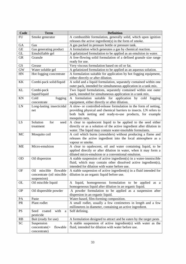
33

Code Term Definition FU Smoke generator A combustible formulation, generally solid, which upon ignition

releases the active ingredient(s) in the form of smoke. GA Gas A gas packed in pressure bottle or pressure tank. GE Gas generating product A formulation which generates a gas by chemical reaction. GL Emulsifiable gel A gelatinized formulation to be applied as an emulsion in water. GR Granule A free-flowing solid formulation of a defined granule size range

ready for use. GS Grease Very viscous formulation based on oil or fat. GW Water soluble gel A gelatinized formulation to be applied as an aqueous solution. HN Hot fogging concentrate A formulation suitable for application by hot fogging equipment,

either directly or after dilution. KK Combi-pack solid/liquid A solid and a liquid formulation, separately contained within one

outer pack, intended for simultaneous application in a tank mix. KL Combi-pack

liquid/liquid Two liquid formulations, separately contained within one outer pack, intended for simultaneous application in a tank mix.

KN Cold fogging concentrate

A formulation suitable for application by cold fogging equipment, either directly or after dilution.

LN Long-lasting insecticidal net

A slow- or controlled-release formulation in the form of netting, providing physical and chemical barriers to insects. LN refers to both bulk netting and ready-to-use products, for example mosquito nets.

LS Solution for seed treatment

A clear to opalescent liquid to be applied to the seed either directly or as a solution of the active ingredient after dilution in water. The liquid may contain water-insoluble formulants.

MC Mosquito coil A coil which burns (smoulders) without producing a flame and releases the active ingredient into the local atmosphere as a vapour or smoke.

ME Micro-emulsion A clear to opalescent, oil and water containing liquid, to be applied directly or after dilution in water, when it may form a diluted micro-emulsion or a conventional emulsion.

OD Oil dispersion A stable suspension of active ingredient(s) in a water-immiscible fluid, which may contain other dissolved active ingredient(s), intended for dilution with water before use.

OF Oil miscible flowable concentrate (oil miscible suspension)

A stable suspension of active ingredient(s) in a fluid intended for dilution in an organic liquid before use.

OL Oil miscible liquid A liquid, homogeneous formulation to be applied as a homogeneous liquid after dilution in an organic liquid.

OP Oil dispersible powder A powder formulation to be applied as a suspension after dispersion in an organic liquid.

PA Paste Water-based, film-forming composition. PR Plant rodlet A small rodlet, usually a few centimetres in length and a few

millimetres in diameter, containing an active ingredient. PS Seed coated with a

pesticide Self defining.

RB Bait (ready for use) A formulation designed to attract and be eaten by the target pests SC Suspension

concentrate(= flowable concentrate)

A stable suspension of active ingredient(s) with water as the fluid, intended for dilution with water before use.

34

Code Term Definition SD Suspension concentrate

for direct application A stable suspension of active ingredient(s) in a fluid, which may contain other dissolved active ingredient(s), intended for direct application, to rice paddies, for example.

SE Suspo-emulsion A fluid, heterogeneous formulation consisting of a stable dispersion of active ingredients in the form of solid particles and fine globules in a continuous water phase.

SG Water soluble granule A formulation consisting of granules to be applied as a true solution of the active ingredient after dissolution in water, but which may contain insoluble inert ingredients.

SL Soluble concentrate A clear to opalescent liquid to be applied as a solution of the active ingredient after dilution in water. The liquid may contain water-insoluble formulants.

SO Spreading oil Formulation designed to form a surface layer on application to water.

SP Water soluble powder A powder formulation to be applied as a true solution of the active ingredient after dissolution in water, but which may contain insoluble inert ingredients.

ST Water soluble tablet Formulation in form of tablets to be used individually, to form a solution of the active ingredient after disintegration in water. The formulation may contain water-insoluble formulants.

SU Ultra-low volume (ULV) suspension

A suspension ready for use through ULV equipment.

TB Tablet Pre-formed solids of uniform shape and dimensions, usually circular, with either flat or convex faces, the distance between faces being less than the diameter.

TC Technical material A material resulting from a manufacturing process comprising the active ingredient, together with associated impurities. This may contain small amounts of necessary additives.

TK Technical concentrate A material resulting from a manufacturing process comprising the active ingredient, together with associated impurities. This may contain small amounts of necessary additives and appropriate diluents.

UL Ultra-low volume (ULV) liquid

A homogeneous liquid ready for use through ULV equipment.

VP Vapour releasing product

A formulation containing one or more volatile active ingredients, the vapours of which are released into the air. Evaporation rate is normally controlled by using suitable formulations and/or dispensers.

WG Water dispersible granules

A formulation consisting of granules to be applied after disintegration and dispersion in water.

WP Wettable powder A powder formulation to be applied as a suspension after dispersion in water.

WS Water dispersible powder for slurry seed treatment

A powder to be dispersed at high concentration in water before application as a slurry to the seed.

WT Water dispersible tablet Formulation in the form of tablets to be used individually, to form a dispersion of the active ingredient after disintegration in water.

XX Others Temporary categorization of all other formulations not listed

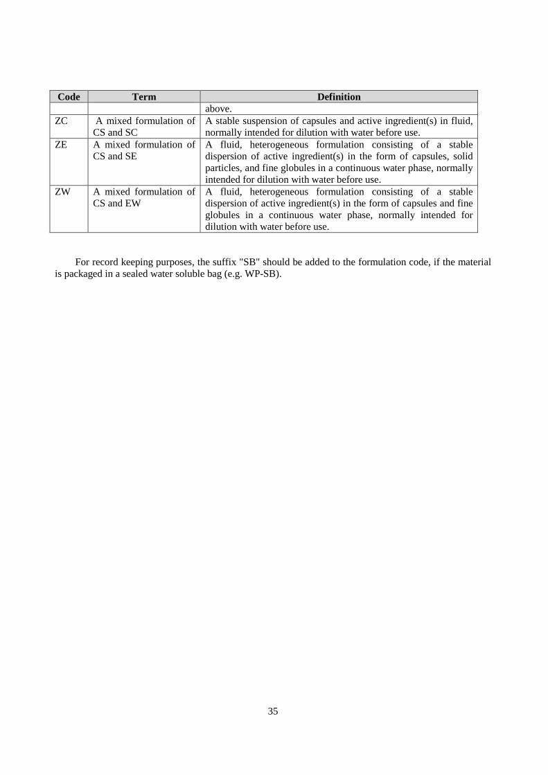
35

Code Term Definition above.

ZC A mixed formulation of CS and SC

A stable suspension of capsules and active ingredient(s) in fluid, normally intended for dilution with water before use.

ZE A mixed formulation of CS and SE

A fluid, heterogeneous formulation consisting of a stable dispersion of active ingredient(s) in the form of capsules, solid particles, and fine globules in a continuous water phase, normally intended for dilution with water before use.

ZW A mixed formulation of CS and EW

A fluid, heterogeneous formulation consisting of a stable dispersion of active ingredient(s) in the form of capsules and fine globules in a continuous water phase, normally intended for dilution with water before use.

For record keeping purposes, the suffix "SB" should be added to the formulation code, if the material is packaged in a sealed water soluble bag (e.g. WP-SB).

36

Table 3: Proposed Number of Residue Trials for Comprehensive Submissions

Minimum number of Supervised Field Trials Conducted at cGAP

Crop1 US

Additional Canadian (where US trials do not overlap)

EU2 JP3 AUS NZ Other Total After 40% reduction4

Acerola (Barbados cherry) 1 4 2 7 8 Alfalfa 12 6 F 2 4 24 15 Almond 5 4 2 6 2 19 13 Apple 16 4 16 6 8 6 56 35 Apple, Sugar 2 4 2 8 8 Apricot 5 2 12 2 6 2 29 20 Arracacha 2 4 2 8 8 Artichoke, Globe 3 4 2 2 11 8 Artichoke, Jerusalem 3 4 2 2 11 8 Asparagus 8 1 6 2 4 4 25 16 Atemoya 1 4 2 2 9 8 Avocado 5 4 2 8 2 21 14 Banana 5 4 2 8 19 12 Barley 12 9 16 3 8 4 52 31 Bean, Dried 12 3 16 2 2 35 23 Bean, Edible Podded 8 16 2 4 30 19 Bean, Lima, Dried 3 16 2 2 23 16 Bean, Lima, Green 8 16 2 8 2 36 24 Bean, Mung 3 2 2 7 8 Bean, Snap 8 2 2 2 14 11 Bean, Succulent Shelled 8 16 3 2 29 19 Beet, Garden 5 1 12 2 2 22 15 Blackberry 5 1 4 2 2 14 10 Blueberry 8 3 4 2 4 2 23 15 Bok choi 2 2 2 6 8 Boysenberry 2 4 2 2 10 8 Broccoli 8 4 6 3 8 4 33 20 Broccoli, Chinese (gai lon) 2 2 2 6 8 Brussels Sprouts 3 2 6 2 4 2 19 14 Buckwheat 5 6 2 2 15 11 Cabbage 8 4 12 6 8 4 42 25 Cabbage, Chinese 3 4 6 2 15 10 Cacao Bean (cocoa) 3 2 5 8 Calabaza 2 2 4 8 Calamondin (Codex: mandarin) 1 2 3 8 Canola 8 9 16 2 8 2 45 29 Cantaloupe 8 12 2 8 2 32 21 Capsicum (pepper) 8 8 Carambola 2 4 2 2 10 8 Carob 3 4 2 9 8 Carrot 8 4 16 6 8 4 46 28 Cassava, bitter or sweet 2 4 2 2 10 8 Cauliflower 8 3 16 2 8 2 39 26 Celery 8 4 6 3 4 4 29 17 Cherry, Sweet 8 1 12 2 3 4 30 19

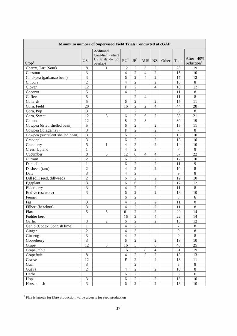
37

Minimum number of Supervised Field Trials Conducted at cGAP

Crop1 US

Additional Canadian (where US trials do not overlap)

EU2 JP3 AUS NZ Other Total After 40% reduction4

Cherry, Tart (Sour) 8 1 12 2 3 2 28 19 Chestnut 3 4 2 4 2 15 10 Chickpea (garbanzo bean) 3 6 2 4 2 17 12 Chicory 2 4 2 2 10 8 Clover 12 F 2 4 18 12 Coconut 5 4 2 11 8 Coffee 5 2 4 11 8 Collards 5 6 2 2 15 11 Corn, Field 20 16 2 2 4 44 28 Corn, Pop 3 2 5 8 Corn, Sweet 12 3 6 3 6 2 33 21 Cotton 12 8 2 8 30 19 Cowpea (dried shelled bean) 5 6 2 2 15 11 Cowpea (forage/hay) 3 F 2 2 7 8 Cowpea (succulent shelled bean) 3 6 2 2 13 10 Crabapple 3 6 2 2 13 10 Cranberry 5 1 4 2 2 14 10 Cress, Upland 1 4 2 7 8 Cucumber 8 3 12 6 4 4 37 22 Currant 2 6 2 2 12 10 Dandelion 1 6 2 2 11 9 Dasheen (taro) 2 4 2 2 10 8 Date 3 4 2 9 8 Dill (dill seed, dillweed) 2 6 2 2 12 10 Eggplant 3 6 6 2 17 12 Elderberry 3 4 2 2 11 8 Endive (escarole) 3 6 2 2 13 10 Fennel 6 2 8 6 Fig 3 4 2 2 11 8 Filbert (hazelnut) 3 4 2 2 11 8 Flax 5 5 62 2 2 20 14 Fodder beet 16 2 4 22 14 Garlic 3 2 6 2 2 15 12 Genip (Codex: Spanish lime) 1 4 2 7 8 Ginger 2 4 3 9 8 Ginseng 3 4 2 9 8 Gooseberry 3 6 2 2 13 10 Grape 12 3 16 3 6 40 25 Grape, table 16 3 8 4 31 19 Grapefruit 8 4 2 2 2 18 13 Grasses 12 F 2 4 18 11 Guar 3 2 5 8 Guava 2 4 2 2 10 8 Herbs 6 2 8 6 Hops 3 6 2 2 13 10 Horseradish 3 6 2 2 13 10

2 Flax is known for fibre production, value given is for seed production

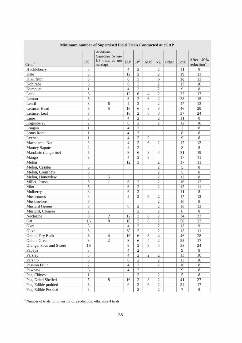
38

Minimum number of Supervised Field Trials Conducted at cGAP

Crop1 US

Additional Canadian (where US trials do not overlap)

EU2 JP3 AUS NZ Other Total After 40% reduction4

Huckleberry 3 4 2 2 11 8 Kale 3 12 2 2 19 13 Kiwi fruit 3 6 3 6 18 12

Kohlrabi 3 6 2 2 13 10 Kumquat 1 4 2 2 9 8 Leek 3 12 6 4 2 27 17 Lemon 5 8 2 6 2 23 15 Lentil 3 6 4 2 2 17 12 Lettuce, Head 8 5 16 6 8 3 46 29 Lettuce, Leaf 8 16 2 8 3 37 24 Lime 3 4 2 2 11 8 Loganberry 2 6 2 2 12 10 Longan 1 4 2 7 8 Lotus Root 1 4 3 8 8 Lychee 1 4 2 2 9 8 Macadamia Nut 3 4 2 6 2 17 12 Mamey Sapote 2 4 2 8 8 Mandarin (tangerine) 5 8 6 8 4 31 19 Mango 3 4 2 8 17 11 Melon 12 3 2 17 11 Melon, Casaba 3 2 5 8 Melon, Crenshaw 3 2 5 8 Melon, Honeydew 5 5 2 12 8 Millet, Proso 5 1 6 2 2 16 12 Mint 5 6 2 2 15 11 Mulberry 3 6 2 11 8 Mushrooms 3 4 2 6 2 17 12 Muskmelons 8 2 10 8 Mustard Greens 8 6 2 2 18 13 Mustard, Chinese 2 2 2 6 8 Nectarine 8 2 12 2 8 2 34 23 Oat 16 8 16 2 6 2 50 33 Okra 5 4 2 2 13 9 Olive 3 83 2 2 15 11 Onion, Dry Bulb 8 4 16 6 8 4 46 28 Onion, Green 3 2 8 6 4 2 25 17 Orange, Sour and Sweet 16 8 2 8 4 38 24 Papaya 3 4 2 9 8 Parsley 3 4 2 2 2 13 10 Parsnip 3 6 2 2 13 10 Passion Fruit 2 4 2 2 10 8 Pawpaw 3 4 2 9 8 Pea, Chinese 1 2 2 5 8 Pea, Dried Shelled 5 8 16 2 8 2 41 27 Pea, Edible podded 8 6 2 6 2 24 17 Pea, Edible Podded 3 2 2 7 8

3 Number of trials for olives for oil production; otherwise 4 trials

39

Minimum number of Supervised Field Trials Conducted at cGAP

Crop1 US

Additional Canadian (where US trials do not overlap)

EU2 JP3 AUS NZ Other Total After 40% reduction4

Pea, Field (Austrian Winter) (forage/hay) 3 F 2 8 2 15 11 Pea, Succulent Shelled (Pea, Garden, Succulent) 8 4 16 2 2 32 21 Peach 12 4 12 3 8 4 43 25 Peanut 12 3 4 2 8 29 18 Peanut, Perennial 3 2 5 8 Pear 8 4 16 6 8 4 46 28 Pecan 5 4 2 4 2 17 11 Pepper, (other than bell) 3 2 2 7 8 Pepper, Bell 8 4 16 3 2 33 21 Persimmon 3 4 6 4 17 10 Pimento 2 4 2 2 10 8 Pineapple 8 4 2 14 9 Pistachio 3 4 2 9 8 Plantain 3 4 2 9 8 Plum 8 1 16 2 8 2 37 25 Pomegranate 3 4 2 9 8 Potato 16 10 16 6 8 4 60 37 Pumpkin 5 4 6 2 4 2 23 15 Quince 3 6 2 2 13 10 Radish 5 1 6 2 2 16 12 Radish, Oriental (daikon) 2 6 2 10 8 Rapeseed 3 16 2 2 23 16 Raspberry, Black and Red 5 6 2 2 17 11 Rhubarb 2 1 6 2 2 13 11 Rice 16 8 6 6 36 23 Rice, Wild 5 4 2 11 8 Rutabaga 3 2 64 2 2 13 11 Rye 5 2 16 2 2 27 19 Safflower 5 2 4 2 2 15 11 Sainfoin 3 F 2 2 7 8 Salsify 3 6 2 2 13 10 Sesame 3 4 2 9 8 Shallot 1 6 2 2 11 9 Sorghum, Grain 12 8 2 6 2 30 20 Soybean (dried) 20 1 16 6 8 4 55 34 Spices 6 2 8 6 Spinach 8 3 6 6 2 25 17 Squash, Summer 8 4 12 2 4 30 18 Squash, Winter 5 6 3 2 16 11 Strawberry 8 3 16 3 8 4 42 26 Sugar Beet 12 6 16 3 2 39 25 Sugarcane 8 3 8 19 12 Sunflower 8 2 16 2 8 2 38 26 Sweet Potato 8 4 6 2 20 13

4 See turnip

40

Minimum number of Supervised Field Trials Conducted at cGAP

Crop1 US

Additional Canadian (where US trials do not overlap)

EU2 JP3 AUS NZ Other Total After 40% reduction4

Swiss Chard 3 6 2 2 13 10 Tangelo 3 4 2 2 11 8 Tanier (cocoyam) 2 2 4 8 Tea 6 6 8 Tobacco 3 5 4 2 2 16 11 Tomato 16 11 16 6 8 4 61 38 Triticale 16 2 4 2 24 16 Turnip, root 5 6 3 4 18 11 Turnip, tops (leaves) 5 6 3 2 16 11 Walnut, Black and English 3 6 2 2 13 10 Watercress 2 6 2 2 12 10 Watermelon 8 16 6 4 2 36 23 Wheat 20 13 16 6 12 4 71 43 Yam, True 3 4 3 2 12 8

1 Crops to be reconsidered after Codex classification is finalised. 2 Number of trials for fodder crops (marked F) in Europe not yet harmonised, although criteria are

available that allow specifying number of trials i. e. cultivation area (ha) and production (t).

In case no number is given the mentioned crop is not widely grown in Europe. The number of trials necessary depends on criteria described in the EU Guidelines on comparability, extrapolation, group tolerances and data requirements for setting MRLs.

In addition, the new data requirement as described in Regulation (EU) No 283/2013 allow a reduction of the number of trials for minor crops that are growing in both European residue zones and where the GAP is the same. In this case six trials are sufficient instead of eight which is reflected in the above table.

3 The Japanese government revised the requirements for the number of trials of residue data, depending on the production volume and consumption of each crop/commodity, within the review of pesticide registration scheme. From 1st April in 2014, the minimum number of trials is six for major crops and three for semi-major crops, respectively. The minimum number of trials remains two for minor crops.

4 To take into account that no reduction on two trials in an OECD country is possible and that a minimum of eight trials for a comprehensive submission is required.

41

ANNEXES

Three Annexes are provided in a separate publication ENV/JM/MONO(2016)XX/ANN

Annex 1: Background Information to Chapter 1. Crop Grouping (including two Appendices)

Annex 2: Background Information to Chapter 2. Extrapolations

Annex 3: Background Information to Chapter 3. Proportionality (including four Appendices)