ODTK Theory and Algorithms
426
Orbit Determination Tool Kit Theory & Algorithms 1 James R. Wright, et al. May 1, 2013 1 c Analytical Graphics, Inc., 2002 through 2012. All Rights Reserved.
-
Upload
bala-murugan -
Category
Documents
-
view
274 -
download
16
description
Orbit determination
Transcript of ODTK Theory and Algorithms
Orbit Determination Tool KitTheory & Algorithms1
James R. Wright, et al.
May 1, 2013
1 c Analytical Graphics, Inc., 2002 through 2012. All Rights Reserved.

ii

Contents
0.1 Preface . . . . . . . . . . . . . . . . . . . . . . . . . . . . . . . . xx0.2 Acknowledgements . . . . . . . . . . . . . . . . . . . . . . . . . . xx0.3 US Patents . . . . . . . . . . . . . . . . . . . . . . . . . . . . . . xx
1 Introduction 11.1 Orbit Determination Classes . . . . . . . . . . . . . . . . . . . . . 1
1.1.1 IOD Methods . . . . . . . . . . . . . . . . . . . . . . . . . 21.1.2 LS Methods . . . . . . . . . . . . . . . . . . . . . . . . . . 21.1.3 SP Methods . . . . . . . . . . . . . . . . . . . . . . . . . . 21.1.4 "Batch Filter" (Sequential LS) Methods . . . . . . . . . . 31.1.5 Optimal Orbit Determination . . . . . . . . . . . . . . . . 3
1.2 Notation . . . . . . . . . . . . . . . . . . . . . . . . . . . . . . . . 41.2.1 Coordinate Frames . . . . . . . . . . . . . . . . . . . . . . 41.2.2 Spacecraft Vectors and Components . . . . . . . . . . . . 71.2.3 Numerical Orbit Propagation . . . . . . . . . . . . . . . . 8
1.3 Mathematical Operators for SP Methods . . . . . . . . . . . . . . 91.3.1 Subscript Notation . . . . . . . . . . . . . . . . . . . . . . 91.3.2 Nonlinear Operators . . . . . . . . . . . . . . . . . . . . . 101.3.3 Linear Operators . . . . . . . . . . . . . . . . . . . . . . . 10
1.4 Document Partition . . . . . . . . . . . . . . . . . . . . . . . . . 11
I Optimal Orbit Determination 13
2 Optimal Orbit Determination (OOD) 152.1 De�nitions . . . . . . . . . . . . . . . . . . . . . . . . . . . . . . . 15
2.1.1 State Estimate Reference for Linearization of SP Methods 152.1.2 Local Linearization . . . . . . . . . . . . . . . . . . . . . . 162.1.3 Global Linearization . . . . . . . . . . . . . . . . . . . . . 162.1.4 Observability . . . . . . . . . . . . . . . . . . . . . . . . . 162.1.5 Completeness . . . . . . . . . . . . . . . . . . . . . . . . . 162.1.6 Optimal Orbit Determination . . . . . . . . . . . . . . . . 162.1.7 Discussion . . . . . . . . . . . . . . . . . . . . . . . . . . . 17
iii

iv CONTENTS
3 Fundamental Theorem of Estimation 193.1 Gaussian Probability Density Function . . . . . . . . . . . . . . . 19
3.1.1 Sample Data . . . . . . . . . . . . . . . . . . . . . . . . . 193.1.2 Multidimensional Gaussian Random Variable . . . . . . . 19
3.2 Gaussian Cumulative Distribution Function . . . . . . . . . . . . 203.2.1 Central Limit Theorem . . . . . . . . . . . . . . . . . . . 213.2.2 Multidimensional Gaussian Random Variable . . . . . . . 22
3.3 Short Version of Fundamental Theorem . . . . . . . . . . . . . . 223.4 Complete Version of Fundamental Theorem . . . . . . . . . . . . 223.5 Comparison to Least Squares . . . . . . . . . . . . . . . . . . . . 23
4 Kalman�s Approach 254.1 Linearization . . . . . . . . . . . . . . . . . . . . . . . . . . . . . 254.2 State Estimate Error Model . . . . . . . . . . . . . . . . . . . . . 264.3 Integral Equation . . . . . . . . . . . . . . . . . . . . . . . . . . . 26
4.3.1 Gauss-Markov Sequence . . . . . . . . . . . . . . . . . . . 274.4 Time Update Algorithm . . . . . . . . . . . . . . . . . . . . . . . 27
4.4.1 State Error Covariance for Filter Time Update . . . . . . 274.5 Measurement Update Algorithm . . . . . . . . . . . . . . . . . . 28
5 Optimal Sequential Filter 315.1 State Estimate Error Model . . . . . . . . . . . . . . . . . . . . . 315.2 Integral Equation . . . . . . . . . . . . . . . . . . . . . . . . . . . 325.3 State Error Covariance for Filter Time Update . . . . . . . . . . 325.4 Approximate Error-Model Solutions . . . . . . . . . . . . . . . . 33
5.4.1 Gravity Solution . . . . . . . . . . . . . . . . . . . . . . . 335.4.2 Air-Drag Solution . . . . . . . . . . . . . . . . . . . . . . 335.4.3 Solar Pressure Solution . . . . . . . . . . . . . . . . . . . 34
5.5 Filter Time Update Algorithm . . . . . . . . . . . . . . . . . . . 345.6 Filter Measurement Update . . . . . . . . . . . . . . . . . . . . . 34
5.6.1 Measurement Editing . . . . . . . . . . . . . . . . . . . . 345.6.2 Supplementary Editor . . . . . . . . . . . . . . . . . . . . 355.6.3 Filter Initialization . . . . . . . . . . . . . . . . . . . . . . 355.6.4 Filter Divergence . . . . . . . . . . . . . . . . . . . . . . . 35
6 Fixed Interval Sequential Smoother 376.1 Smoother Initialization . . . . . . . . . . . . . . . . . . . . . . . . 376.2 Notation for Smoother Nonlinear State Transition . . . . . . . . 386.3 Smoother Sequential Equations . . . . . . . . . . . . . . . . . . . 38
6.3.1 Transition Smoothed State Estimate Backwards . . . . . 386.3.2 Incorporate Filter Estimate and Covariance at Time tk . 386.3.3 Prepare to Calculate Smoother Covariance . . . . . . . . 386.3.4 Smoother Covariance . . . . . . . . . . . . . . . . . . . . . 386.3.5 Notes . . . . . . . . . . . . . . . . . . . . . . . . . . . . . 396.3.6 Example for k = L� 1 . . . . . . . . . . . . . . . . . . . . 39
6.4 Filter-Smoother Consistency Test . . . . . . . . . . . . . . . . . . 39

CONTENTS v
6.4.1 Test . . . . . . . . . . . . . . . . . . . . . . . . . . . . . . 406.5 Smoother Matrix Inversions . . . . . . . . . . . . . . . . . . . . . 40
7 Variable-Lag Sequential Smoother 417.1 Introduction . . . . . . . . . . . . . . . . . . . . . . . . . . . . . . 417.2 General Application . . . . . . . . . . . . . . . . . . . . . . . . . 42
7.2.1 ODTK LEO Simulation . . . . . . . . . . . . . . . . . . . 437.3 Impulsive Maneuvers . . . . . . . . . . . . . . . . . . . . . . . . . 437.4 Required Properties . . . . . . . . . . . . . . . . . . . . . . . . . 447.5 Properties Available . . . . . . . . . . . . . . . . . . . . . . . . . 45
7.5.1 Linear . . . . . . . . . . . . . . . . . . . . . . . . . . . . . 457.5.2 Extension . . . . . . . . . . . . . . . . . . . . . . . . . . . 467.5.3 Nonlinear . . . . . . . . . . . . . . . . . . . . . . . . . . . 46
7.6 Kalman Filter . . . . . . . . . . . . . . . . . . . . . . . . . . . . . 477.6.1 Time Update . . . . . . . . . . . . . . . . . . . . . . . . . 477.6.2 Measurement Update . . . . . . . . . . . . . . . . . . . . 48
7.7 Carlton-Rauch Fixed-Epoch Smoother . . . . . . . . . . . . . . . 497.7.1 FES Initialization . . . . . . . . . . . . . . . . . . . . . . 497.7.2 Measurement at tj = tk+1 . . . . . . . . . . . . . . . . . . 507.7.3 Measurements at tj = tk+1; tk+2; : : : . . . . . . . . . . . . 51
7.8 Frazer Fixed-Epoch Smoother . . . . . . . . . . . . . . . . . . . . 517.8.1 FES Initialization . . . . . . . . . . . . . . . . . . . . . . 517.8.2 Measurement at tj = tk+1 . . . . . . . . . . . . . . . . . . 51
8 State-Space Changes 538.1 Problem De�nition . . . . . . . . . . . . . . . . . . . . . . . . . . 53
8.1.1 Structure of VLS Algorithms . . . . . . . . . . . . . . . . 548.2 Handling Discontinuities by the Filter . . . . . . . . . . . . . . . 54
8.2.1 State Contraction . . . . . . . . . . . . . . . . . . . . . . 548.2.2 State Expansion . . . . . . . . . . . . . . . . . . . . . . . 568.2.3 Simultaneous Contraction and Expansion . . . . . . . . . 568.2.4 Stability Properties of the Covariance Contraction . . . . 56
8.3 Smoothing Algorithms . . . . . . . . . . . . . . . . . . . . . . . . 588.3.1 Fixed-Interval Smoothing (RTS) . . . . . . . . . . . . . . 588.3.2 Fixed-Point Smoothing (Carlton-Rauch) . . . . . . . . . . 598.3.3 Fixed-Point Smoother (Meditch, Anderson-Moore) . . . . 598.3.4 McReynolds Multi-point Smoother . . . . . . . . . . . . . 62
8.4 Handling Filter Discontinuities with Smoothers . . . . . . . . . . 638.4.1 Fixed-Interval Smoothing with Discontinuities . . . . . . 638.4.2 Fixed-Point Smoothing (Carlton-Rauch) with Discontinu-
ities . . . . . . . . . . . . . . . . . . . . . . . . . . . . . . 658.4.3 Fixed-Point Smoothing (Fraser) with Discontinuities . . . 668.4.4 Multi-Point Smoothing with Discontinuities . . . . . . . . 67
vi CONTENTS
9 Relative Orbit Errors 699.1 Simultaneous Orbit Determination . . . . . . . . . . . . . . . . . 699.2 Orbit Di¤erence Error Covariance . . . . . . . . . . . . . . . . . 70
10 Orbit Errors in Keplerian Variables 71
11 Time Grids 73
II Stochastic Sequences 75
12 Stochastic Sequences for OOD 7712.1 A Scalar Exponential Gauss-Markov Sequence . . . . . . . . . . . 77
12.1.1 Deterministic Transitivity with Time . . . . . . . . . . . . 7812.1.2 Stationary Variance . . . . . . . . . . . . . . . . . . . . . 7912.1.3 Propagation Time Extrema . . . . . . . . . . . . . . . . . 8012.1.4 Input Control . . . . . . . . . . . . . . . . . . . . . . . . . 8012.1.5 Estimation . . . . . . . . . . . . . . . . . . . . . . . . . . 8112.1.6 Stationarity . . . . . . . . . . . . . . . . . . . . . . . . . . 82
12.2 The Vasicek Stochastic Sequence . . . . . . . . . . . . . . . . . . 8212.2.1 Transition Matrix �� . . . . . . . . . . . . . . . . . . . . . 8412.2.2 Units . . . . . . . . . . . . . . . . . . . . . . . . . . . . . 8512.2.3 Volatility . . . . . . . . . . . . . . . . . . . . . . . . . . . 8512.2.4 Drift . . . . . . . . . . . . . . . . . . . . . . . . . . . . . . 8512.2.5 Mean . . . . . . . . . . . . . . . . . . . . . . . . . . . . . 8512.2.6 Second Moments . . . . . . . . . . . . . . . . . . . . . . . 8512.2.7 Summary . . . . . . . . . . . . . . . . . . . . . . . . . . . 8712.2.8 Example . . . . . . . . . . . . . . . . . . . . . . . . . . . . 8712.2.9 Sequential Estimation . . . . . . . . . . . . . . . . . . . . 88
12.3 Other Stochastic Sequences . . . . . . . . . . . . . . . . . . . . . 9212.3.1 Brownian Motion . . . . . . . . . . . . . . . . . . . . . . . 9212.3.2 White Noise . . . . . . . . . . . . . . . . . . . . . . . . . . 9412.3.3 Clocks . . . . . . . . . . . . . . . . . . . . . . . . . . . . . 96
III Accelerations 97
13 Accelerations 9913.1 Two Body Acceleration . . . . . . . . . . . . . . . . . . . . . . . 9913.2 Total Acceleration . . . . . . . . . . . . . . . . . . . . . . . . . . 99
14 Earth Gravity 10114.1 Geopotential . . . . . . . . . . . . . . . . . . . . . . . . . . . . . 10114.2 Legendre Functions . . . . . . . . . . . . . . . . . . . . . . . . . . 102
14.2.1 Legendre Polynomials of First Kind . . . . . . . . . . . . 10214.2.2 Associated Legendre Functions of First Kind . . . . . . . 103
14.3 Auto-Covariance Function on a Sphere . . . . . . . . . . . . . . . 103

CONTENTS vii
14.3.1 From Angle to Time . . . . . . . . . . . . . . . . . . . . . 10514.3.2 Covariance Function R (0) . . . . . . . . . . . . . . . . . . 10514.3.3 Auto-correlation Function . . . . . . . . . . . . . . . . . . 105
14.4 Acceleration Errors on a Sphere . . . . . . . . . . . . . . . . . . . 10614.4.1 Computational Problem . . . . . . . . . . . . . . . . . . . 10714.4.2 Solution to Computational Problem . . . . . . . . . . . . 10814.4.3 The Double Integral . . . . . . . . . . . . . . . . . . . . . 10814.4.4 Markov Property . . . . . . . . . . . . . . . . . . . . . . . 10814.4.5 Inertial Frame . . . . . . . . . . . . . . . . . . . . . . . . 10914.4.6 Stochastic Characterization . . . . . . . . . . . . . . . . . 11014.4.7 Implementation . . . . . . . . . . . . . . . . . . . . . . . . 110
14.5 Perigee-Apogee Weighting . . . . . . . . . . . . . . . . . . . . . . 11014.5.1 Weighting Functions . . . . . . . . . . . . . . . . . . . . . 111
14.6 New Method . . . . . . . . . . . . . . . . . . . . . . . . . . . . . 11214.6.1 Splines . . . . . . . . . . . . . . . . . . . . . . . . . . . . . 11214.6.2 Sample Covariance Validation . . . . . . . . . . . . . . . . 11214.6.3 GRACE . . . . . . . . . . . . . . . . . . . . . . . . . . . . 11214.6.4 EGM96 . . . . . . . . . . . . . . . . . . . . . . . . . . . . 113
14.7 Simulate Gravity Coe¢ cient Errors . . . . . . . . . . . . . . . . . 11314.7.1 Covariance Matrix Representations . . . . . . . . . . . . . 11314.7.2 Simulation of x . . . . . . . . . . . . . . . . . . . . . . . . 11414.7.3 A Useful Example . . . . . . . . . . . . . . . . . . . . . . 115
15 Lunar Gravity 11715.1 Lunar Prospector . . . . . . . . . . . . . . . . . . . . . . . . . . . 117
16 Atmospheric Drag and Lift 11916.1 King-Hele Unit Vector K . . . . . . . . . . . . . . . . . . . . . . 11916.2 Orthonormal Vector Basis [a] . . . . . . . . . . . . . . . . . . . . 12016.3 Drag-Lift Acceleration . . . . . . . . . . . . . . . . . . . . . . . . 12116.4 Air-Drag Acceleration . . . . . . . . . . . . . . . . . . . . . . . . 121
16.4.1 Drag Acceleration . . . . . . . . . . . . . . . . . . . . . . 12116.5 Ballistic Coe¢ cient Errors . . . . . . . . . . . . . . . . . . . . . . 12216.6 Atmospheric Density Errors . . . . . . . . . . . . . . . . . . . . . 122
16.6.1 Relative Error Base-Line Model on Air-Density . . . . . . 12316.6.2 Gauss-Markov Sequence on Air-Density Relative Error . . 12416.6.3 Propagation of State Estimate . . . . . . . . . . . . . . . 12416.6.4 State Estimate Error . . . . . . . . . . . . . . . . . . . . . 12516.6.5 Process Noise Covariance . . . . . . . . . . . . . . . . . . 12516.6.6 Transform From Perigee Height to Current Height . . . . 12716.6.7 Orbit Error Covariance . . . . . . . . . . . . . . . . . . . 128

viii CONTENTS
17 Solar Photon Pressure 13117.1 Coordinate Frame for Solar Pressure . . . . . . . . . . . . . . . . 13117.2 Solar Pressure Acceleration . . . . . . . . . . . . . . . . . . . . . 132
17.2.1 Notation . . . . . . . . . . . . . . . . . . . . . . . . . . . . 13317.2.2 Conservation of Linear Momentum . . . . . . . . . . . . . 13317.2.3 Spherical Surface Di¤use Re�ection . . . . . . . . . . . . 13417.2.4 Spherical Surface Perfect Absorption . . . . . . . . . . . . 134
17.3 Eclipse Modeling . . . . . . . . . . . . . . . . . . . . . . . . . . . 13417.3.1 Selection . . . . . . . . . . . . . . . . . . . . . . . . . . . . 13417.3.2 Baker�s Dual-Cone Eclipse Model . . . . . . . . . . . . . . 13517.3.3 Earth Radius . . . . . . . . . . . . . . . . . . . . . . . . . 137
17.4 Stochastic Solar Pressure Error Model . . . . . . . . . . . . . . . 137
18 GPS Solar Pressure Models 13918.1 GSPM.04a . . . . . . . . . . . . . . . . . . . . . . . . . . . . . . . 13918.2 GSPM.04ae . . . . . . . . . . . . . . . . . . . . . . . . . . . . . . 13918.3 AeroT20 . . . . . . . . . . . . . . . . . . . . . . . . . . . . . . . . 13918.4 AeroT30 . . . . . . . . . . . . . . . . . . . . . . . . . . . . . . . . 14018.5 Estimation . . . . . . . . . . . . . . . . . . . . . . . . . . . . . . 140
19 Spacecraft Thrusting 14119.1 Impulsive Maneuver Model . . . . . . . . . . . . . . . . . . . . . 141
19.1.1 Trajectory . . . . . . . . . . . . . . . . . . . . . . . . . . . 14119.1.2 Trajectory Error Covariance . . . . . . . . . . . . . . . . . 14219.1.3 Time of Centroid tC . . . . . . . . . . . . . . . . . . . . . 143
19.2 Impulsive Maneuver Error Covariance . . . . . . . . . . . . . . . 14419.2.1 Notation . . . . . . . . . . . . . . . . . . . . . . . . . . . . 14419.2.2 Time Relations . . . . . . . . . . . . . . . . . . . . . . . . 14419.2.3 Covariance . . . . . . . . . . . . . . . . . . . . . . . . . . 145
19.3 Impulsive Maneuver Covariance . . . . . . . . . . . . . . . . . . . 14619.3.1 Discussion . . . . . . . . . . . . . . . . . . . . . . . . . . . 147
19.4 Finite Maneuver Model . . . . . . . . . . . . . . . . . . . . . . . 14819.4.1 Kinematics . . . . . . . . . . . . . . . . . . . . . . . . . . 14819.4.2 Dynamics . . . . . . . . . . . . . . . . . . . . . . . . . . . 14919.4.3 Stochastic Sequences . . . . . . . . . . . . . . . . . . . . . 14919.4.4 Estimation . . . . . . . . . . . . . . . . . . . . . . . . . . 150
IV Spacecraft Attitude 151
20 Attitude Modeling 15320.1 Antenna Phase Center Estimation . . . . . . . . . . . . . . . . . 153

CONTENTS ix
V State Error Transition 155
21 Transitive Partial Derivatives 15721.1 State Error Transition Function . . . . . . . . . . . . . . . . . . . 15721.2 Position & Velocity Partials . . . . . . . . . . . . . . . . . . . . . 157
21.2.1 Two-Body Transition Matrix . . . . . . . . . . . . . . . . 15821.2.2 Variational Equations Transition Matrix . . . . . . . . . . 158
21.3 Air-Drag Partials . . . . . . . . . . . . . . . . . . . . . . . . . . . 16121.4 Solar Pressure Partials . . . . . . . . . . . . . . . . . . . . . . . . 162
VI Ground Location Estimation 163
VII Measurements 167
22 Tracking Station Kinematics 16922.1 Introduction . . . . . . . . . . . . . . . . . . . . . . . . . . . . . . 16922.2 The Earth-Centered Unit Sphere . . . . . . . . . . . . . . . . . . 17022.3 Ellipse in Plane of f1 and f3 . . . . . . . . . . . . . . . . . . . . . 172
22.3.1 Normal Vector n�pf�. . . . . . . . . . . . . . . . . . . . 173
22.3.2 Geodetic Latitude . . . . . . . . . . . . . . . . . . . . . . 17322.3.3 Normal Vector n (') . . . . . . . . . . . . . . . . . . . . . 17422.3.4 Station Height Above Ellipse . . . . . . . . . . . . . . . . 17422.3.5 R . . . . . . . . . . . . . . . . . . . . . . . . . . . . . . . 17522.3.6 Geocentric vs Geodetic Latitude . . . . . . . . . . . . . . 17522.3.7 Topocentric Geodetic Vector Basis [N] . . . . . . . . . . . 17922.3.8 Topocentric Geocentric Vector Basis [M] . . . . . . . . . 180
22.4 Earth Fixed Vector Basis [e] . . . . . . . . . . . . . . . . . . . . . 18122.4.1 From [f ] to [e] . . . . . . . . . . . . . . . . . . . . . . . . 18122.4.2 The Ellipsoid . . . . . . . . . . . . . . . . . . . . . . . . . 18222.4.3 Station Vector . . . . . . . . . . . . . . . . . . . . . . . . 18322.4.4 Normal Vector n (') . . . . . . . . . . . . . . . . . . . . . 18322.4.5 R . . . . . . . . . . . . . . . . . . . . . . . . . . . . . . . 184
23 Angles 18523.1 Unit Range Vector . . . . . . . . . . . . . . . . . . . . . . . . . . 18523.2 Azimuth and Elevation . . . . . . . . . . . . . . . . . . . . . . . . 185
23.2.1 Construct L from Azimuth and Elevation . . . . . . . . . 18623.2.2 Construct Azimuth and Elevation from L . . . . . . . . . 18723.2.3 Partial Derivatives of Azimuth and Elevation . . . . . . . 18723.2.4 Construct Le from Azimuth and Elevation . . . . . . . . 18923.2.5 Construct Azimuth and Elevation from Le . . . . . . . . . 190
23.3 Direction Cosines . . . . . . . . . . . . . . . . . . . . . . . . . . . 19023.3.1 Construct Direction Cosines LF1 and L
F2 from L . . . . . 192
23.3.2 Partial Derivatives of Direction Cosines LF1 and LF2 . . . 192

x CONTENTS
23.4 X/Y Angles . . . . . . . . . . . . . . . . . . . . . . . . . . . . . . 19323.4.1 X/Y East-West Reference Frame . . . . . . . . . . . . . . 19323.4.2 X/Y North-South Reference Frame . . . . . . . . . . . . 19423.4.3 X/Y Z Reference Frame . . . . . . . . . . . . . . . . . . 19423.4.4 X and Y Angles . . . . . . . . . . . . . . . . . . . . . . . 19423.4.5 Partial Derivatives of X and Y Angles . . . . . . . . . . . 195
23.5 Ground Based Tracker . . . . . . . . . . . . . . . . . . . . . . . . 19523.5.1 Partials . . . . . . . . . . . . . . . . . . . . . . . . . . . . 195
23.6 Space Based Tracker . . . . . . . . . . . . . . . . . . . . . . . . . 19723.7 Earth Ellipsoid Values . . . . . . . . . . . . . . . . . . . . . . . . 197
23.7.1 NIMA/NASA EGM96 . . . . . . . . . . . . . . . . . . . . 19723.7.2 On the EGM96 Ellipsoid . . . . . . . . . . . . . . . . . . 198
24 Range 19924.1 Classical Two-Way Range . . . . . . . . . . . . . . . . . . . . . . 201
24.1.1 Notation . . . . . . . . . . . . . . . . . . . . . . . . . . . . 20124.1.2 De�nitions . . . . . . . . . . . . . . . . . . . . . . . . . . 20124.1.3 Special Relativity . . . . . . . . . . . . . . . . . . . . . . . 20224.1.4 Calculation . . . . . . . . . . . . . . . . . . . . . . . . . . 20224.1.5 Complete Representation . . . . . . . . . . . . . . . . . . 203
24.2 Satellite to Satellite Two-Way Range . . . . . . . . . . . . . . . . 20324.3 Bi-Static Range (One-Way) . . . . . . . . . . . . . . . . . . . . . 203
25 Doppler 20525.1 Classical Two-Way Doppler . . . . . . . . . . . . . . . . . . . . . 206
25.1.1 Notation . . . . . . . . . . . . . . . . . . . . . . . . . . . . 20625.1.2 De�nitions . . . . . . . . . . . . . . . . . . . . . . . . . . 20625.1.3 Expressions for Uplink Range-Rate . . . . . . . . . . . . . 20725.1.4 Expressions for Downlink Range-Rate . . . . . . . . . . . 20825.1.5 Two-Way Range-Rate . . . . . . . . . . . . . . . . . . . . 20925.1.6 Two-Way Doppler Frequency Equation . . . . . . . . . . 21025.1.7 Two-Way Phase Count Equation . . . . . . . . . . . . . . 21125.1.8 Observed Frequency . . . . . . . . . . . . . . . . . . . . . 21125.1.9 Measurement Names . . . . . . . . . . . . . . . . . . . . . 212
25.2 SCF ARTS Doppler . . . . . . . . . . . . . . . . . . . . . . . . . 21225.2.1 Complete Representation . . . . . . . . . . . . . . . . . . 21325.2.2 Partial Derivatives . . . . . . . . . . . . . . . . . . . . . . 213
25.3 NASA STDN Doppler . . . . . . . . . . . . . . . . . . . . . . . . 21425.3.1 Observed Range Rate . . . . . . . . . . . . . . . . . . . . 21425.3.2 Doppler Representation from the Observed Range Rate
Equation . . . . . . . . . . . . . . . . . . . . . . . . . . . 215

CONTENTS xi
26 Troposphere 21726.1 Troposphere Range . . . . . . . . . . . . . . . . . . . . . . . . . . 217
26.1.1 Zenith Component . . . . . . . . . . . . . . . . . . . . . . 21726.1.2 Mapping Function . . . . . . . . . . . . . . . . . . . . . . 220
26.2 Partial Pressure Measurements . . . . . . . . . . . . . . . . . . . 22326.3 Atmospheric Thermodynamics . . . . . . . . . . . . . . . . . . . 224
26.3.1 State Variables . . . . . . . . . . . . . . . . . . . . . . . . 22426.3.2 Ideal Gas Law . . . . . . . . . . . . . . . . . . . . . . . . 22526.3.3 Relative Humidity and Partial Pressures . . . . . . . . . . 225
26.4 Troposphere Range Error . . . . . . . . . . . . . . . . . . . . . . 22626.4.1 Propagation Variance for Relative Troposphere Range Error22726.4.2 Sequential Estimation . . . . . . . . . . . . . . . . . . . . 228
26.5 SCF �RC Model . . . . . . . . . . . . . . . . . . . . . . . . . . . . 22826.5.1 Tropospheric Range Model (�RC) . . . . . . . . . . . . . . 22826.5.2 Doppler . . . . . . . . . . . . . . . . . . . . . . . . . . . . 229
27 Ionosphere 23127.1 Range . . . . . . . . . . . . . . . . . . . . . . . . . . . . . . . . . 23127.2 Doppler . . . . . . . . . . . . . . . . . . . . . . . . . . . . . . . . 232
27.2.1 SCF ARTS Doppler (Range-Rate) . . . . . . . . . . . . . 232
28 TDOA 23328.1 Ground-based TDOA (Ground to Spacecraft to Ground) . . . . . 233
28.1.1 Ground-based TDOA light time algorithm . . . . . . . . . 23328.1.2 Complete Representation . . . . . . . . . . . . . . . . . . 235
28.2 Ground TDOA (Spacecraft to Ground) . . . . . . . . . . . . . . . 23528.2.1 Ground TDOA light time algorithm . . . . . . . . . . . . 23528.2.2 Complete Representation . . . . . . . . . . . . . . . . . . 236
28.3 Ground-based single di¤erenced TDOA (Ground to Spacecraft toGround) . . . . . . . . . . . . . . . . . . . . . . . . . . . . . . . . 236
28.4 Space-based TDOA (Ground to Spacecraft) . . . . . . . . . . . . 23628.4.1 Space-based TDOA light time algorithm . . . . . . . . . . 23728.4.2 Complete Representation . . . . . . . . . . . . . . . . . . 237
29 FDOA 23929.1 Ground-based FDOA (Ground to Spacecraft to Ground) . . . . . 239
29.1.1 Doppler shift . . . . . . . . . . . . . . . . . . . . . . . . . 23929.1.2 Frequency of arrival . . . . . . . . . . . . . . . . . . . . . 24029.1.3 Complete Representation . . . . . . . . . . . . . . . . . . 240
29.2 Ground FDOA (Spacecraft to Ground) . . . . . . . . . . . . . . . 24129.2.1 Frequency of arrival . . . . . . . . . . . . . . . . . . . . . 24129.2.2 Complete Representation . . . . . . . . . . . . . . . . . . 241
29.3 Ground-based single di¤erenced FDOA (Ground to Spacecraft toGround) . . . . . . . . . . . . . . . . . . . . . . . . . . . . . . . . 241
29.4 Space-based FDOA (Ground to Spacecraft) . . . . . . . . . . . . 24229.4.1 Frequency of arrival . . . . . . . . . . . . . . . . . . . . . 242

xii CONTENTS
29.4.2 Complete Representation . . . . . . . . . . . . . . . . . . 242
30 TDOA Dot 24330.1 Ground-based TDOA Dot (Ground to Spacecraft to Ground) . . 243
30.1.1 Range rate . . . . . . . . . . . . . . . . . . . . . . . . . . 24330.1.2 Rate of change of time of arrival . . . . . . . . . . . . . . 24430.1.3 Complete Representation . . . . . . . . . . . . . . . . . . 244
30.2 Space-based TDOA Dot (Ground to Spacecraft) . . . . . . . . . 24430.2.1 Rate of change of time of arrival . . . . . . . . . . . . . . 24530.2.2 Complete Representation . . . . . . . . . . . . . . . . . . 245
31 FDOA Dot 24731.1 Ground FDOA Dot . . . . . . . . . . . . . . . . . . . . . . . . . . 247
31.1.1 Frequency of arrival rate . . . . . . . . . . . . . . . . . . . 24731.1.2 Complete Representation . . . . . . . . . . . . . . . . . . 248
32 DSN Range and Total Count Phase 24932.1 Sequential Range . . . . . . . . . . . . . . . . . . . . . . . . . . . 24932.2 Total Count Phase . . . . . . . . . . . . . . . . . . . . . . . . . . 24932.3 Doppler . . . . . . . . . . . . . . . . . . . . . . . . . . . . . . . . 25032.4 Antenna Corrections . . . . . . . . . . . . . . . . . . . . . . . . . 25032.5 Media Corrections . . . . . . . . . . . . . . . . . . . . . . . . . . 25032.6 Solar Corona Model . . . . . . . . . . . . . . . . . . . . . . . . . 250
33 Clock Modeling 25133.1 Introduction . . . . . . . . . . . . . . . . . . . . . . . . . . . . . . 25133.2 Time . . . . . . . . . . . . . . . . . . . . . . . . . . . . . . . . . . 252
33.2.1 Variable t . . . . . . . . . . . . . . . . . . . . . . . . . . . 25233.2.2 Constant � . . . . . . . . . . . . . . . . . . . . . . . . . . 252
33.3 ODTK Simulator Clock Time Update . . . . . . . . . . . . . . . 25233.4 ODTK Filter Clock Time Update . . . . . . . . . . . . . . . . . . 253
33.4.1 State . . . . . . . . . . . . . . . . . . . . . . . . . . . . . . 25333.4.2 Covariance . . . . . . . . . . . . . . . . . . . . . . . . . . 253
33.5 Allan Variance . . . . . . . . . . . . . . . . . . . . . . . . . . . . 25333.5.1 Covariance on Clock Phase . . . . . . . . . . . . . . . . . 25433.5.2 Simulations . . . . . . . . . . . . . . . . . . . . . . . . . . 25533.5.3 Filter Time Update for Clock . . . . . . . . . . . . . . . . 25833.5.4 State Estimate Parameters . . . . . . . . . . . . . . . . . 258
33.6 Zucca-Tavella Clock Model . . . . . . . . . . . . . . . . . . . . . 259
VIII Least Squares (LS) 261
34 LS Inputs 26334.1 Input Values . . . . . . . . . . . . . . . . . . . . . . . . . . . . . 26334.2 Initial Calculated Values . . . . . . . . . . . . . . . . . . . . . . . 264

CONTENTS xiii
34.2.1 Measurement Residuals . . . . . . . . . . . . . . . . . . . 26434.2.2 Partial Derivatives . . . . . . . . . . . . . . . . . . . . . . 265
35 Least Squares Solutions 26735.1 LS Normal Equation and Solution . . . . . . . . . . . . . . . . . 267
35.1.1 Linearization . . . . . . . . . . . . . . . . . . . . . . . . . 26735.2 Remove the Squaring Operation . . . . . . . . . . . . . . . . . . 26835.3 Solution by Triangularization of B . . . . . . . . . . . . . . . . . 269
35.3.1 Solution Overview . . . . . . . . . . . . . . . . . . . . . . 269
36 Least Squares Inadequacies 27136.1 LS Measurement Residuals . . . . . . . . . . . . . . . . . . . . . 27136.2 Incomplete LS Model . . . . . . . . . . . . . . . . . . . . . . . . . 27136.3 Least Squares State Error Covariance . . . . . . . . . . . . . . . 27136.4 Batch Simultaneity . . . . . . . . . . . . . . . . . . . . . . . . . . 27236.5 Schmidt�s Analysis of Least Squares . . . . . . . . . . . . . . . . 272
36.5.1 A Practical Experiment . . . . . . . . . . . . . . . . . . . 27236.6 Gibb�s E¤ect . . . . . . . . . . . . . . . . . . . . . . . . . . . . . 273
37 Tracking Data Editing 27537.1 Tracking Data Editor Identi�cation . . . . . . . . . . . . . . . . . 27637.2 Minimum Number of Data Sets Editor . . . . . . . . . . . . . . . 27737.3 Minimum Time Span Editor . . . . . . . . . . . . . . . . . . . . . 27737.4 Tracking Loop Flag Editor . . . . . . . . . . . . . . . . . . . . . . 27737.5 Gross Raw Data Editor . . . . . . . . . . . . . . . . . . . . . . . 27737.6 Minimum Elevation Editor . . . . . . . . . . . . . . . . . . . . . 27837.7 Sliding Raw Data Polynomial Editor . . . . . . . . . . . . . . . . 27837.8 Kepler Element Editor . . . . . . . . . . . . . . . . . . . . . . . . 278
37.8.1 Kepler Element Bounds Criterion . . . . . . . . . . . . . . 27937.8.2 m =M = 3 . . . . . . . . . . . . . . . . . . . . . . . . . . 28137.8.3 m =M = 4 . . . . . . . . . . . . . . . . . . . . . . . . . . 28137.8.4 m =M = 5 . . . . . . . . . . . . . . . . . . . . . . . . . . 28137.8.5 m � 6 . . . . . . . . . . . . . . . . . . . . . . . . . . . . . 28237.8.6 Kepler Element Statistics Criterion . . . . . . . . . . . . . 282
37.9 Second Di¤erence Editor Using IOD . . . . . . . . . . . . . . . . 28337.10Convergence Criteria . . . . . . . . . . . . . . . . . . . . . . . . . 283
37.10.1Residual RMS Convergence Criterion Using IOD . . . . . 28337.10.2Residual RMS Convergence Criterion After First Correction284
37.11Residual Editor . . . . . . . . . . . . . . . . . . . . . . . . . . . . 28537.12Least Squares Solution . . . . . . . . . . . . . . . . . . . . . . . . 285
37.12.1Exceed Maximum Iteration Count Editor . . . . . . . . . 28537.13Manual Editor . . . . . . . . . . . . . . . . . . . . . . . . . . . . 28537.14Select A New Station Pass . . . . . . . . . . . . . . . . . . . . . . 28537.15Measurement Biases . . . . . . . . . . . . . . . . . . . . . . . . . 285

xiv CONTENTS
IX Initial Orbit Determination 287
38 IOD Methods 28938.1 Common Modeling Limitations . . . . . . . . . . . . . . . . . . . 289
38.1.1 Two-Body Dynamics . . . . . . . . . . . . . . . . . . . . . 28938.1.2 Measurement Outliers . . . . . . . . . . . . . . . . . . . . 289
38.2 Common Equations for IOD . . . . . . . . . . . . . . . . . . . . . 29038.2.1 Equation of Motion . . . . . . . . . . . . . . . . . . . . . 29038.2.2 Triangle Geometry . . . . . . . . . . . . . . . . . . . . . . 290
39 Herrick-Gibbs 29139.1 Position Vectors . . . . . . . . . . . . . . . . . . . . . . . . . . . 291
39.1.1 Taylor�s Series . . . . . . . . . . . . . . . . . . . . . . . . 291
40 Gooding 29540.1 Description . . . . . . . . . . . . . . . . . . . . . . . . . . . . . . 295
40.1.1 Guess Range Values . . . . . . . . . . . . . . . . . . . . . 29540.1.2 Lambert . . . . . . . . . . . . . . . . . . . . . . . . . . . . 29540.1.3 Gooding . . . . . . . . . . . . . . . . . . . . . . . . . . . . 296
40.2 A Priori Orbit Information . . . . . . . . . . . . . . . . . . . . . 29740.2.1 Near-Circular Orbits . . . . . . . . . . . . . . . . . . . . . 29740.2.2 High Eccentricity Orbits . . . . . . . . . . . . . . . . . . . 298
40.3 White Noise . . . . . . . . . . . . . . . . . . . . . . . . . . . . . . 29840.4 Tropospheric E¤ects . . . . . . . . . . . . . . . . . . . . . . . . . 29840.5 Inspection of Kepler Orbit Element Values . . . . . . . . . . . . . 29840.6 Multiple Solutions from Each Set of Distinct Measurement Sets . 29840.7 Least Squares . . . . . . . . . . . . . . . . . . . . . . . . . . . . . 299
X Tracking and Data Relay Satellite System (TDRSS)301
41 TDRSS Range and Doppler 30341.1 TDRSS Range Vectors . . . . . . . . . . . . . . . . . . . . . . . . 30341.2 Range Sum . . . . . . . . . . . . . . . . . . . . . . . . . . . . . . 304
41.2.1 Range Elements . . . . . . . . . . . . . . . . . . . . . . . 30541.2.2 Range Sum De�nition . . . . . . . . . . . . . . . . . . . . 30541.2.3 Range Sum Time Tag . . . . . . . . . . . . . . . . . . . . 30541.2.4 Construction of the Range Sum Representation . . . . . . 305
41.3 Range Sum Partial Derivatives . . . . . . . . . . . . . . . . . . . 30641.3.1 Eliminate Light-Time . . . . . . . . . . . . . . . . . . . . 30641.3.2 Simpli�ed Expressions . . . . . . . . . . . . . . . . . . . . 30741.3.3 Di¤erentials . . . . . . . . . . . . . . . . . . . . . . . . . . 30741.3.4 LEO Satellite Range Sum Partials . . . . . . . . . . . . . 30741.3.5 TDRS Range Sum Partials . . . . . . . . . . . . . . . . . 309
41.4 Doppler Measurements . . . . . . . . . . . . . . . . . . . . . . . . 31041.5 DopplerPartials . . . . . . . . . . . . . . . . . . . . . . . . . . . . 311

CONTENTS xv
41.5.1 LEO Satellite Doppler Partials . . . . . . . . . . . . . . . 31141.5.2 TDRS Doppler Partials . . . . . . . . . . . . . . . . . . . 312
42 One-Way Return-Link Doppler 313
XI Global Positioning System (GPS) Low Earth Orbit(LEO) Receivers 315
43 Pseudo-Range Filtering 31743.1 Introduction . . . . . . . . . . . . . . . . . . . . . . . . . . . . . . 317
43.1.1 Pseudo-Range Option . . . . . . . . . . . . . . . . . . . . 31743.2 USER GPS Pseudo-Range . . . . . . . . . . . . . . . . . . . . . . 318
43.2.1 Pseudo-Range . . . . . . . . . . . . . . . . . . . . . . . . . 31843.2.2 Range Measurement Time Notation . . . . . . . . . . . . 31843.2.3 Time Di¤erences . . . . . . . . . . . . . . . . . . . . . . . 31843.2.4 Receiver Clock Errors . . . . . . . . . . . . . . . . . . . . 31843.2.5 Receiver Proper Time less Receiver Coordinate Time (User
Spacecraft) . . . . . . . . . . . . . . . . . . . . . . . . . . 31943.2.6 Coordinate Time Di¤erence . . . . . . . . . . . . . . . . . 32043.2.7 Transmitter Coordinate Time less Transmitter Proper Time
(NAVSTAR) . . . . . . . . . . . . . . . . . . . . . . . . . 32043.2.8 Transmitter Clock Error . . . . . . . . . . . . . . . . . . . 321
43.3 Schwarzschild Metric . . . . . . . . . . . . . . . . . . . . . . . . . 32243.3.1 Proper Time vs Coordinate Time . . . . . . . . . . . . . . 32343.3.2 Time Integrals . . . . . . . . . . . . . . . . . . . . . . . . 32343.3.3 JPL Model . . . . . . . . . . . . . . . . . . . . . . . . . . 325
43.4 Group Delay Di¤erential . . . . . . . . . . . . . . . . . . . . . . . 32543.5 Remove Ionospheric Range . . . . . . . . . . . . . . . . . . . . . 325
43.5.1 Proof . . . . . . . . . . . . . . . . . . . . . . . . . . . . . 32643.5.2 Phase Count . . . . . . . . . . . . . . . . . . . . . . . . . 326
43.6 GPS Range First-Di¤erences . . . . . . . . . . . . . . . . . . . . 32743.6.1 Notation . . . . . . . . . . . . . . . . . . . . . . . . . . . . 32743.6.2 C/A Code Range Representation . . . . . . . . . . . . . . 32743.6.3 First Di¤erence . . . . . . . . . . . . . . . . . . . . . . . . 327
43.7 Partial Derivatives for HANU . . . . . . . . . . . . . . . . . . . . 32843.7.1 ICD-GPS-208 18 April 1983 . . . . . . . . . . . . . . . . . 32843.7.2 Partials . . . . . . . . . . . . . . . . . . . . . . . . . . . . 32843.7.3 Map HANU Covariance P to GPS Measurement Covari-
ance Py . . . . . . . . . . . . . . . . . . . . . . . . . . . . 32943.7.4 Initial Di¤erential Equations for Variations in Range and
Range-Rate . . . . . . . . . . . . . . . . . . . . . . . . . . 33043.7.5 Position and Velocity Variations in Inertial Component
Matrices . . . . . . . . . . . . . . . . . . . . . . . . . . . . 33243.7.6 Partials . . . . . . . . . . . . . . . . . . . . . . . . . . . . 332

xvi CONTENTS
44 GPS Carrier Phase Count 33544.1 Introduction . . . . . . . . . . . . . . . . . . . . . . . . . . . . . . 335
44.1.1 BlackJack GPS Receiver . . . . . . . . . . . . . . . . . . . 33644.2 Implementation . . . . . . . . . . . . . . . . . . . . . . . . . . . . 336
44.2.1 Estimation of Clock Parameters . . . . . . . . . . . . . . 33644.2.2 L1 Phase Count Measurements . . . . . . . . . . . . . . . 33744.2.3 L1, L2 Phase Count Measurements . . . . . . . . . . . . . 33744.2.4 Partial Derivatives . . . . . . . . . . . . . . . . . . . . . . 337
44.3 Notation . . . . . . . . . . . . . . . . . . . . . . . . . . . . . . . . 33744.3.1 Time . . . . . . . . . . . . . . . . . . . . . . . . . . . . . . 33744.3.2 Oscillator and Clock . . . . . . . . . . . . . . . . . . . . . 33844.3.3 Generalized Integral . . . . . . . . . . . . . . . . . . . . . 33844.3.4 Doppler Phase Count . . . . . . . . . . . . . . . . . . . . 33844.3.5 Two Types of Phase Count Error . . . . . . . . . . . . . . 339
44.4 Receiver Doppler Algorithm . . . . . . . . . . . . . . . . . . . . . 34044.4.1 NAVSTAR Frequencies . . . . . . . . . . . . . . . . . . . 34044.4.2 Doppler Frequency . . . . . . . . . . . . . . . . . . . . . . 34044.4.3 De�ne Phase Count . . . . . . . . . . . . . . . . . . . . . 34144.4.4 Doppler Shift . . . . . . . . . . . . . . . . . . . . . . . . . 34244.4.5 Phase Count Representation . . . . . . . . . . . . . . . . 34344.4.6 Approximations for �ij . . . . . . . . . . . . . . . . . . . 34444.4.7 USER Orbit Partial Derivatives . . . . . . . . . . . . . . . 345
44.5 Ionosphere . . . . . . . . . . . . . . . . . . . . . . . . . . . . . . . 34644.5.1 Physics . . . . . . . . . . . . . . . . . . . . . . . . . . . . 34644.5.2 Total Electron Content . . . . . . . . . . . . . . . . . . . 34744.5.3 Validation . . . . . . . . . . . . . . . . . . . . . . . . . . . 349
44.6 Final Forms for Phase Count . . . . . . . . . . . . . . . . . . . . 34944.6.1 Alternate Representation . . . . . . . . . . . . . . . . . . 350
44.7 Ionosphere Removal . . . . . . . . . . . . . . . . . . . . . . . . . 35144.7.1 Ionosphere-Free White Noise Variance for �NEi
j (Cycles) . 35344.7.2 Ionosphere-Free White Noise Variance for �� (cm) . . . . 355
44.8 First Di¤erences on NEij . . . . . . . . . . . . . . . . . . . . . . . 358
44.8.1 Remove USER Clock Phase Perturbations . . . . . . . . . 35844.8.2 Root-Variance Mappings . . . . . . . . . . . . . . . . . . . 359
44.9 Example . . . . . . . . . . . . . . . . . . . . . . . . . . . . . . . . 36044.10Partials and Covariance . . . . . . . . . . . . . . . . . . . . . . . 360
44.10.1Single Frequency . . . . . . . . . . . . . . . . . . . . . . . 36044.10.2Two-Frequency Ionosphere Removal . . . . . . . . . . . . 36144.10.3First Di¤erences on NEi
j . . . . . . . . . . . . . . . . . . . 36244.11Receiver Clock Error Model . . . . . . . . . . . . . . . . . . . . . 363
44.11.1Covariance on Clock Phase . . . . . . . . . . . . . . . . . 36344.11.2Simulations . . . . . . . . . . . . . . . . . . . . . . . . . . 36544.11.3Filter Time Update for Receiver Clock . . . . . . . . . . . 36644.11.4State Estimate Parameters . . . . . . . . . . . . . . . . . 367

CONTENTS xvii
45 GPS Navigation Solution 36945.1 Introduction . . . . . . . . . . . . . . . . . . . . . . . . . . . . . . 36945.2 Algorithm . . . . . . . . . . . . . . . . . . . . . . . . . . . . . . . 369
XII Global Positioning System (GPS) Ground Receivers373
46 GPS Composite Clock 37546.1 GOMA-E . . . . . . . . . . . . . . . . . . . . . . . . . . . . . . . 37546.2 Tutorial . . . . . . . . . . . . . . . . . . . . . . . . . . . . . . . . 375
46.2.1 Simulation Narrative . . . . . . . . . . . . . . . . . . . . . 37546.2.2 Similarity in Clock Parameter Variations . . . . . . . . . 37646.2.3 Optimal Estimation of the UVCC . . . . . . . . . . . . . 37746.2.4 Real World Application . . . . . . . . . . . . . . . . . . . 377
XIII Appendices 383
A. The Least Squares Quadratic 385
B. Sequential Least Squares 387
C. Ad-Hoc Batch Filter 391
D. Kalman�s Model Equation 395.0.5 Measurements at tj = tk+1; tk+2; : : : . . . . . . . . . . . . 395

xviii CONTENTS

List of Figures
3.1 Gaussian Density Function f(x) . . . . . . . . . . . . . . . . . . . 203.2 Gaussian Distribution Function F(x) . . . . . . . . . . . . . . . . 21
7.1 Variable Lag Smoother with EKF and FES . . . . . . . . . . . . 427.2 Estimation of Velocity at Fixed Epochs with EKF and FES . . . 43
12.1 Exponential Transition-Correlation Function and Half-Life Func-tion . . . . . . . . . . . . . . . . . . . . . . . . . . . . . . . . . . 88
12.2 24 Unbiased Vasicek Sequences . . . . . . . . . . . . . . . . . . . 8912.3 24 Biased Vasicek Sequences . . . . . . . . . . . . . . . . . . . . . 89
16.1 Sigma for Relative Error in Air Density . . . . . . . . . . . . . . 123
17.1 Dual-Cone Eclipse Geometry . . . . . . . . . . . . . . . . . . . . 13617.2 Baker�s Solar Obscura . . . . . . . . . . . . . . . . . . . . . . . . 136
19.1 Unit Thrust Referred to Maneuver Frame . . . . . . . . . . . . . 148
22.1 Station Longitude Rotation . . . . . . . . . . . . . . . . . . . . . 17122.2 Geocentric Station Vector Basis . . . . . . . . . . . . . . . . . . . 17222.3 Station Position Vector . . . . . . . . . . . . . . . . . . . . . . . 17522.4 Geocentric vs Geodetic . . . . . . . . . . . . . . . . . . . . . . . . 17622.5 Vector Basis for Angles Measurements . . . . . . . . . . . . . . . 17922.6 Latitude Rotation . . . . . . . . . . . . . . . . . . . . . . . . . . 18122.7 Latitude Di¤erence Rotation . . . . . . . . . . . . . . . . . . . . 182
23.1 Azimuth-Elevation Description . . . . . . . . . . . . . . . . . . . 18623.2 Direction Cosines Description . . . . . . . . . . . . . . . . . . . . 19123.3 Unit Range Vector Right Ascension & Declination . . . . . . . . 196
33.1 Simulated Allan Variance Diagram . . . . . . . . . . . . . . . . . 257
36.1 Position Error vs Least Squares Fit Span . . . . . . . . . . . . . 272
41.1 Four TDRSS Range Vectors . . . . . . . . . . . . . . . . . . . . . 304
xix

xx LIST OF FIGURES
43.1 Earth-USER-NAVSTAR Vector Triangle . . . . . . . . . . . . . . 330
46.1 Sim Phase Dev (units: 1� 10�7s) vs Time (0 - 8) d . . . . . . . 37846.2 Sim & Est Phase Dev (units: 1� 10�7s) vs Time (0 - 8) d . . . . 37946.3 4 Similar Phase Var (units: 1� 10�7s) vs Time (0 - 8) d . . . . . 37946.4 4 Similar Phase Var (units: 1� 10�8s) vs Time (0 - 3) d . . . . . 38046.5 S1 Phase Var & Cov Bounds (units: 1� 10�6s) vs Time (0 - 8) d 38046.6 S1 Phase Var Reduced Cov (units: 1� 10�7s) vs Time (0 - 8) d . 38146.7 S1 Phase Var Reduced Cov (units: 1� 10�9s) vs Time (0 - 8) d . 38146.8 4 Similar Phase Var no IC (units: 1� 10�8s) vs Time (0 - 8) d . 382
0.1 Preface
Analytical Graphics presents here the mathematical speci�cations for its al-gorithms and software used to de�ne new capabilites for orbit determination.These capabilities are referred to as Orbit Determination Tool Kit (ODTK1).The initial purpose for this document was to enable the author to proceed
with the construction of new prototype software for the AGI ODTK methodsof orbit determination. Recording speci�c algorithm de�nitions, and their re-lations to appropriate hardware dynamics and spacecraft trajectory physics,enables and supports algorithm development, review, validation, modi�cation,and communication.This is a living document. Its secondary purpose is to provide relevant
mathematical speci�cations for ODTK users as the algorithms and software aredeveloped.This document is constructed and modi�ed using the Standard LaTeX Book
shell for Scienti�c Workplace 5.5 by MacKichan Software.
0.2 Acknowledgements
I am especially appreciative of the contributions by Dr. James Woodburn toODTK, and to this document. I thank Dick Hujsak and William Chuba foruseful suggestions in development of the �rst di¤erencing algorithm for GPSDoppler carrier phase count measurements.
0.3 US Patents
Patent No. US 6,708,116 B2, Method and Apparatus for Orbit Determination,was granted 16 March 2004.Patent No. US 7,050,002 B1, GPS Carrier Phase Measurement Representa-
tion and Method of Use, was granted 23 May 2006.
1ODTK was previously known as STK/OD.
Chapter 1
Introduction
Orbit determination refers to the estimation of orbits of small objects relativeto primary celestial bodies, given applicable measurements. All useful orbitdetermination methods produce orbit estimates that have errors.
1.1 Orbit Determination Classes
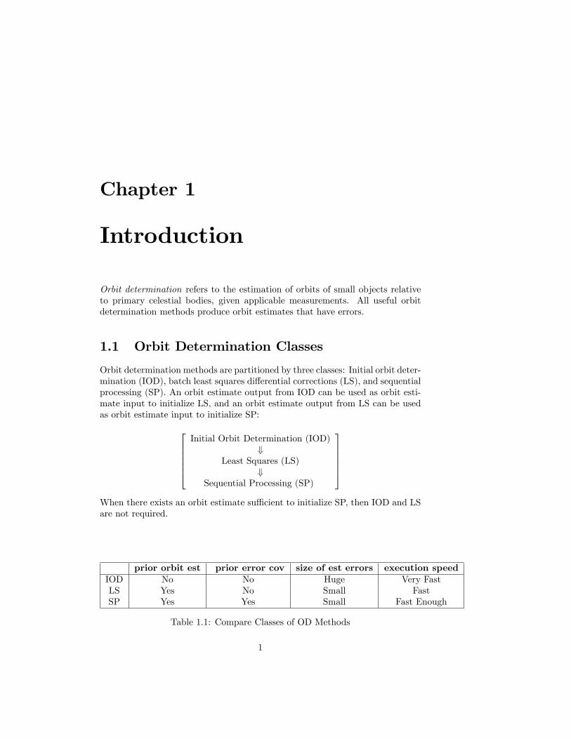
Orbit determination methods are partitioned by three classes: Initial orbit deter-mination (IOD), batch least squares di¤erential corrections (LS), and sequentialprocessing (SP). An orbit estimate output from IOD can be used as orbit esti-mate input to initialize LS, and an orbit estimate output from LS can be usedas orbit estimate input to initialize SP:266664
Initial Orbit Determination (IOD)+
Least Squares (LS)+
Sequential Processing (SP)
377775When there exists an orbit estimate su¢ cient to initialize SP, then IOD and LSare not required.
prior orbit est prior error cov size of est errors execution speedIOD No No Huge Very FastLS Yes No Small FastSP Yes Yes Small Fast Enough
Table 1.1: Compare Classes of OD Methods
1

2 CHAPTER 1. INTRODUCTION
1.1.1 IOD Methods
IOD methods input tracking measurements with tracking platform locations,and output spacecraft orbit estimates. No prior orbit estimate is required,and when used, it is assumed that no prior orbit estimate exists; however, or-bit estimation errors are usually very large. IOD methods are nonlinear andsix-dimensional. Measurement editing is not possible during IOD calculationsbecause no prior orbit estimate exists. IOD methods were derived by various au-thors: LaPlace, Poincaré, Gauss, Lagrange, Lambert, Gibbs, Herrick, Williams,Stumpp, Lancaster, Blanchard, Gooding, and Smith. The orbit determinationprocess is frequently begun, or restarted, with IOD.
1.1.2 LS Methods
The LS method requires the input tracking measurements with tracking plat-form locations and a prior orbit estimate. The LS method outputs a re�nedorbit estimate. Estimation errors are small when compared to IOD outputs.LS methods consist of a sequence of linear LS (di¤erential) corrections wheresequence convergence is de�ned a minimization of the (weighted) sum of squaresof measurement residuals. The sum of squares is represented by Eqs. 35.1, 35.5,and 35.7. Minimization is characterized by Eqs. 35.8 and 35.9. LS methodsproduce re�ned orbit estimates in a batch mode, together with error-covariancematrices that are optimistic; i.e., LS orbit element error variance estimates aretypically too small, relative to truth, by at least an order of magnitude. LSmethods require an inversion of an n � n LS information matrix for each LSiteration, where n is state estimate size. This inversion is problematic whenthe information matrix is ill-conditioned, which is frequently the case in orbitdetermination applications of LS. Operationally, LS may be the only methodused, or, it may be used to initialize SP. The existence of a prior orbit estimateenables operational measurement residual editing, but LS methods frequentlyrequire inspection and manual measurement editing by human intervention. LSalgorithms therefore require elaborate software mechanisms for measurementediting. Gauss reputedly developed LS as early as 1795 and used it to deter-mine the orbit of Ceres in 1801, although he did not publish his account of ituntil the method had already been independently developed and published byLegendre. [25].
1.1.3 SP Methods
SP methods require the input of tracking measurements with tracking plat-form locations, priori state estimates (including an orbit estimate), and a priorstate-error covariance matrix. SP methods output re�ned state estimates in asequential mode. SP �lter methods process forward in time, repeating a re-curring, two-step sequence of �lter time-update of the state estimate and �ltermeasurement-update of the state estimate. The �lter time-update propagatesthe state estimate forward, and the �lter measurement-update incorporates the

1.1. ORBIT DETERMINATION CLASSES 3
next measurement.The recursive sequence requires an important interval of �lter initialization.
Often the state-error covariance is unrealistic during the �lter-initialization timeinterval because the error covariance matrix associated with the a priori orbitestimate is unknown. A signi�cant number of observations must be processedto bring the covariance to a realistic scale. Conceptually, the �lter has beeninitialized once the state covariance becomes realistic; in practice, the �lter isconsidered initialized after having processed a prescribed number of observa-tions.No matrix inversions are performed during �lter calculations. SP smoother
methods process backward in time, repeating a pattern of state-estimate re-�nement using �lter outputs and backwards transition. Matrix inversions arerequired by the smoother algorithm. Computations for both �lter and smootherare dominated most signi�cantly by numerical orbit propagations. The searchfor non-stationary sequential processing was begun by Kalman [48], Bucy [9],Rauch [96], Meditch [76], and others.
1.1.4 "Batch Filter" (Sequential LS) Methods
The batch �lter (Appendix C), BF, is a hybrid algorithm that combines prop-erties of LS with properties of SP. The BF is suggested by inspection of thesequential form of batch least squares (Appendix B). This sequential form ismodi�ed ad hoc by in�ating the covariance associated with previous data. TheBF can be derived by adding a second term ad hoc to the LS quadratic form.The �rst term minimizes the sum of squares of weighted measurement residu-als, while the second term binds the new state estimate to the previous stateestimate. This two-term quadratic form is referred to as a maximum-liklihoodperformance function. Matrix inversion is required by the BF, as in LS. TheBF was proposed by Swerling [103].
1.1.5 Optimal Orbit Determination
Optimal orbit determination (OOD, de�ned in the sequel), depends on the useof an optimal sequential-�lter design. For current time and future time, thesequential �lter output is used directly. For past time, the �lter execution isfollowed by the execution of a �xed interval sequential smoother. The smoothedtrajectory estimates are more accurate than �ltered trajectory estimates.
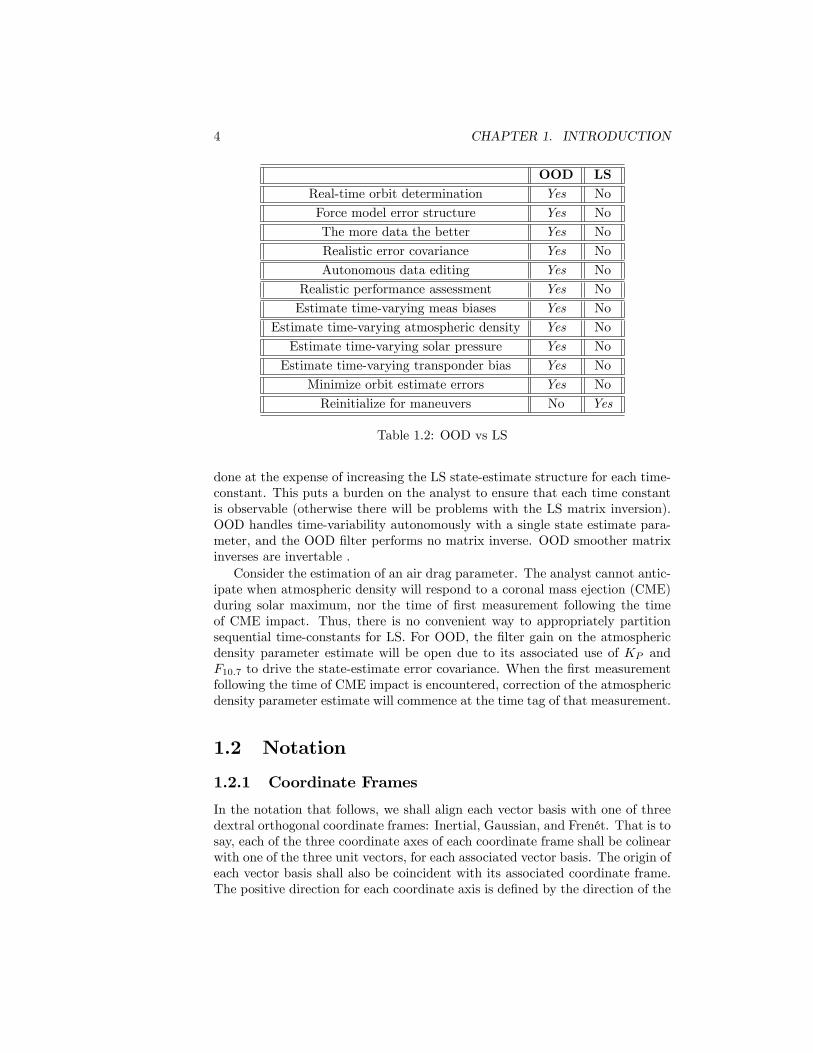
Comparison of OOD with LS
It is useful to compare OOD with LS because many systems use LS to provideoperational end-products. Table 1.2 presents several operational capabilitiesthat distinguish OOD from LS. In particular, OOD allows for the estimationof time-varying parameters, compared to the estimation of static parametersfor LS. In defense of LS, a time-dependent sequence of static parameters maybe estimated with LS, thereby approximating a time-variable; however, this is
4 CHAPTER 1. INTRODUCTION
OOD LSReal-time orbit determination Yes No
Force model error structure Yes No
The more data the better Yes No
Realistic error covariance Yes No
Autonomous data editing Yes No
Realistic performance assessment Yes No
Estimate time-varying meas biases Yes No
Estimate time-varying atmospheric density Yes No
Estimate time-varying solar pressure Yes No
Estimate time-varying transponder bias Yes No
Minimize orbit estimate errors Yes No
Reinitialize for maneuvers No Yes
Table 1.2: OOD vs LS
done at the expense of increasing the LS state-estimate structure for each time-constant. This puts a burden on the analyst to ensure that each time constantis observable (otherwise there will be problems with the LS matrix inversion).OOD handles time-variability autonomously with a single state estimate para-meter, and the OOD �lter performs no matrix inverse. OOD smoother matrixinverses are invertable .Consider the estimation of an air drag parameter. The analyst cannot antic-
ipate when atmospheric density will respond to a coronal mass ejection (CME)during solar maximum, nor the time of �rst measurement following the timeof CME impact. Thus, there is no convenient way to appropriately partitionsequential time-constants for LS. For OOD, the �lter gain on the atmosphericdensity parameter estimate will be open due to its associated use of KP andF10:7 to drive the state-estimate error covariance. When the �rst measurementfollowing the time of CME impact is encountered, correction of the atmosphericdensity parameter estimate will commence at the time tag of that measurement.
1.2 Notation
1.2.1 Coordinate Frames
In the notation that follows, we shall align each vector basis with one of threedextral orthogonal coordinate frames: Inertial, Gaussian, and Frenét. That is tosay, each of the three coordinate axes of each coordinate frame shall be colinearwith one of the three unit vectors, for each associated vector basis. The origin ofeach vector basis shall also be coincident with its associated coordinate frame.The positive direction for each coordinate axis is de�ned by the direction of the

1.2. NOTATION 5
associated unit vector.
Inertial Vector Basis
Let us denote the Earth centered inertial (ECI) orthonormal vector basis forthe International Celestial Reference Frame (ICRF) by the "vectrix" [38]:
[i] =
24 i1i2i3
35 (1.1)
where:
[i]T= (i1; i2; i3) ; (1.2)
where i3 is coincident with the conventional pole (Z-direction) of ICRF, wherei1 and i2 are contained in equatorial plane of the ICRF (where i1 is in the X-direction), and where i2 = i3 � i1.1 It is convenient to associate the origin ofthe inertial vector basis with center of mass of the Earth.
Gaussian Vector Basis
Inertial spacecraft position and velocity vectors are denoted with r and _r. Theorthonormal Gaussian vector basis:
[u] =
24 u1u2u3
35 ; (1.3)
with origin at the spacecraft center of mass, is anchored to the ECI spacecraftposition vector r:
u1 � U = r=r = [i]T
24 U1U2U3
35 (1.4)
where:
r =pr � r (1.5)
Orbit angular momentum h:
h = r� _r (1.6)
enables de�nition of u3:
u3 �W = h=h = [i]T
24 W1
W2
W3
35 (1.7)
1Prior to ODTK 6, the Earth-centered inertial (ECI) frame was aligned with mean equatorand mean equinox at epoch J2000.

6 CHAPTER 1. INTRODUCTION
where:
h =ph � h (1.8)
The triad is completed with:
u2 = u3 � u1 = [i]T24 V1V2V3
35 (1.9)
The rotation 3 x 3 matrix Rui from [i] to [u] :
[u] = Rui [i] (1.10)
where:
Rui =
24 U1 U2 U3V1 V2 V3W1 W2 W3
35 (1.11)
Note that:
[u]T= [i]
TRTui (1.12)
It is convenient to associate the origin of the Gaussian vector basis with centerof mass of a space object.
Frenét Vector Basis
The orthonormal Frenét vector basis:
[f ] =
24 f1f2f3
35 ; (1.13)
with origin at the spacecraft center of mass, is anchored to the ECI spacecraftvelocity vector _r:
f2= _r= _s = [i]T
24 f21f22f23
35 (1.14)
where:
_s =p_r � _r (1.15)
In common with the Gaussian frame, adopt:
f3 = u3 = [i]T
24 f31f32f33
35 (1.16)

1.2. NOTATION 7
The triad is completed with:
f1 = f2 � f3 = [i]T24 f11f12f13
35 (1.17)
The rotation 3 x 3 matrix Rfi from [i] to [f ] :
[f ] = Rfi [i] (1.18)
where:
Rfi =
24 f11 f12 f13f21 f22 f23f31 f32 f33
35 (1.19)
Note that:
[f ]T= [i]
TRTfi (1.20)
It is convenient to associate the origin of the Frenét vector basis with center ofmass of a space object.
1.2.2 Spacecraft Vectors and Components
Position, Velocity, and Acceleration
The spacecraft position, velocity, and acceleration vectors are denoted with r,_r, and �r. Then 3� 1 matrices z, _z, and �z for spacecraft position, velocity, andacceleration components can be represented:
r = [i]Tz (1.21)
_r = [i]T_z (1.22)
�r = [i]T�z: (1.23)
where:
z =
24 z1z2z3
35 (1.24)
_z =
24 _z1_z2_z3
35 (1.25)
�z =
24 �z1�z2�z3
35 (1.26)

8 CHAPTER 1. INTRODUCTION
Position and Velocity Errors
Spacecraft position, velocity, and acceleration vector errors are denoted with �r,� _r, and ��r. Then 3� 1 matrices for instantaneous spacecraft position, velocity,and acceleration error components are represented with:
�r = [i]T�z = [u]
T�y (1.27)
� _r = [i]T� _z = [u]
T� _y (1.28)
��r = [i]T��z = [u]
T��y (1.29)
where:
�z =
24 �z1�z2�z3
35 =24 �r � i1�r � i2�r � i3
35 (1.30)
�y =
24 �y1�y2�y3
35 =24 �r � u1�r � u2�r � u3
35 (1.31)
and where the time derivatives follow by putting appropriate dots over �r;�z;and �y. Insert Eq. 1.12 into Eq. 1.27 to get:
�z = Riu�y (1.32)
�y = Rui�z (1.33)
where:
Riu = RTui (1.34)
1.2.3 Numerical Orbit Propagation
Notation
Concatenate the 3 x 1 position and velocity component arrays z and _z to formthe orbit substate:
Z =
�z_z
�=
26666664z1z2z3_z1_z2_z3
37777775 =26666664Z1Z2Z3Z4Z5Z6
37777775 (1.35)
where Z is dynamic: Z � Z (t).

1.3. MATHEMATICAL OPERATORS FOR SP METHODS 9
Let 'z denote the Variation of Parameters in Universal Variables orbit prop-agator. Given an initial time t0, a �nal time tf , and an acceleration modelu (Z (t) ; t), then 'z propagates Z (t0) from t0 to tf using u (Z (�) ; �) to obtainZ (tf ). This may be expressed as:
Z (tf ) = 'z ftf ; Z (t0) ; t0; u (Z (�) ; �) ; t0 � � � tfg (1.36)
If by 'z we always imply the use of u (Z (t) ; t), then we get a very compactnotation for Variation of Parameters in Universal Variables:
'z ftf ; Z (t0) ; t0g � 'z ftf ; Z (t0) ; t0; u (Z (�) ; �) ; t0 � � � tfg (1.37)
That is:
Z (tf ) = 'z ftf ; Z (t0) ; t0g (1.38)
Ideally, 'z satis�es the nested transitivity property:
Z (tk+2) = 'z ftk+2; Z (tk) ; tkg = 'z ftk+2; 'z ftk+1; Z (tk) ; tkg ; tk+1g(1.39)
Note that 'z is a column matrix with 6 elements:
'z =
2666664'z1'z2'z3...'z6
3777775 (1.40)
1.3 Mathematical Operators for SP Methods
1.3.1 Subscript Notation
State Matrices
The state estimate X is referenced at two separate times by using the notation[76]:
Xjji � X (tj jti) (1.41)
where i, j 2 f0; 1; 2; : : :g. The time tj to the left of the vertical bar denotesthe epoch of X which drives the �lter time-update function. The time ti to theright of the bar denotes the time-tag of the last measurement processed to formX, which drives the �lter measurement-update function. For example, X7j6refers to the state estimate at time t7, given the last measurement processedat time t6, whereas X7j7 refers to the state estimate at time t7, given the last

10 CHAPTER 1. INTRODUCTION
measurement processed at time t7. X7j6 was obtained by �lter time-update ofX6j6 from t6 to t7.Similar notation is used for the state-estimate correction:
�Xjji � �X (tj jti) (1.42)
and the state-estimate-error covariance matrix:
Pjji � P (tj jti) (1.43)
Measurement Matrices
We denote a measurement taken at time tj as yj . We also denote a conditionalmeasurement estimate (representation) at time tj as yjjh.
1.3.2 Nonlinear Operators
Nonlinear operators are required in the state estimate time update and the stateestimate measurement update for SP methods of orbit determination.
State Propagation
Let ' denote a nonlinear operator that propagates the state estimate Xijh fromtime ti to time tj :
Xjjh = 'ntj ; Xijh; ti
o(1.44)
Measurement Representation
Let y (�) denote a nonlinear operator that calculates the measurement represen-tation yjjh, given the state estimate Xjjh:
yjjh = y�Xjjh; tj
�(1.45)
1.3.3 Linear Operators
State Estimate Error Propagation
Let �j;i � � (tj ; ti) denote the linear operator that propagates the state errorestimate �Xijh from time ti to time tj
�Xjjh = �j;i�Xijh (1.46)
where
�j;i =
�@Xj
@Xi
�Xjjh
(1.47)
and where evaluation derives from Xjjh.
1.4. DOCUMENT PARTITION 11
Measurement Residual
Let �yj denote the linear operator that de�nes the measurement residual attime tj :
�yj = yj � yjjh (1.48)
which re�ects the discrepancy between the predicted measurement and theactual measurement at time tj . Some authors refer to �yj as "measurementinnovation".
Measurement/State Partials Jacobian
Let Hj denote the Jacobian of the measurement with respect to the state partialderivatives at time tj :
Hj =
�@yj@Xj
�Xjjh
(1.49)
where evaluation derives from Xjjh.
1.4 Document Partition
This document has the following ordered parts:
1. Optimal Orbit Determination
2. Stochastic Sequences
3. Accelerations
4. Spacecraft Attitude
5. State Error Transition
6. Ground Location Estimation
7. Measurements
8. Deep Space Network (DSN)
9. Least Squares (LS)
10. Initial Orbit Determination (IOD)
11. Tracking and Data Relay Satellite System (TDRSS)
12. Global Positioning System (GPS)
13. Appendices

12 CHAPTER 1. INTRODUCTION

Part I
Optimal OrbitDetermination
13


Chapter 2
Optimal OrbitDetermination (OOD)
As previously mentioned, orbit determination refers to the estimation of orbitsof small objects relative to primary celestial bodies, given applicable measure-ments. But what is optimal orbit determination? The purpose of this chapteris to answer the question.
The adjective optimal refers to most desirable, most favorable, or most sat-isfactory [112]. But most satisfactory to whom? There are choices to make fromavailable orbit determination methods. Should we prefer the fastest methodsor the most accurate? Should we prefer sequential methods or batch methods?Should we minimize the size of the weighted measurement residuals or the sizeof orbit errors? How should we model measurement residuals and orbit errors?
All orbit determination problems are multidimensional and nonlinear,butshould we attempt a multidimensional nonlinear solution directly? Or, shouldwe use a linearization method? If so, is there a preferred method for lineariza-tion?
2.1 De�nitions
2.1.1 State Estimate Reference for Linearization of SPMethods
Evaluation of the measurement representation yjjh de�ned by Eq. 1.45 requiresthe use of some prior state estimate Xjjh, where tj � th and where Xjjh is thestate estimate reference for linearization. A similar requirement is associatedwith Eqs. 1.47 and 1.49.
15

16 CHAPTER 2. OPTIMAL ORBIT DETERMINATION (OOD)
2.1.2 Local Linearization
Let tk and tk+1 � tk be the times of adjacent ordered measurements yk andyk+1, for k 2 f0; 1; 2; : : :g. That is, there are no measurements between yk andyk+1. Then the use of Xk+1jk as the state estimate reference for all linearizationsat time tk+1 de�nes local linearization at time tk+1.The use of any state estimate reference other than Xk+1jk at time tk+1 for
linearization is a non-local linearization at time tk+1.
2.1.3 Global Linearization
Given the integer variable k 2 f0; 1; 2; : : :g and given a �xed non-negative integerj, the use of Xkjj as the state estimate reference for linearization at time tk foreach k is known as global linearization.
2.1.4 Observability
A particular parameter is observable to a particular measurement if and onlyif the sequential processing of that measurement reduces the estimated errorvariance on that parameter.
2.1.5 Completeness
The state estimate structure is complete if and only if all parameters with un-known observable components are included in the state estimate structure.
2.1.6 Optimal Orbit Determination
By optimal orbit determination, the method used to calculate the state estimate(including the orbit estimate) satis�es the following conditions:
1. Sequential processing (SP) is used to account for force modeling errors andmeasurement information in the time order in which they are realized.
2. Sherman�s Theorem is applied [100],[101],[76],[48]. To summarize, theoptimal state estimate correction matrix �X is the expectation of thestate error matrix �X given the measurement residual matrix �y. Thatis: �X = E f�Xj�yg.
3. Linearizations of state-estimate time transition and state-to-measurementrepresentations are local in time, not global.
4. The state estimate structure is complete.
5. All state-estimate models and state-estimate-error model approximationsare derived from the appropriate physics of sensors and force modeling.

2.1. DEFINITIONS 17
6. All measurement models and measurement-error model approximationsare derived from the appropriate sensor hardware de�nitions and associ-ated physics, and measurement sensor performance.
7. Necessary conditions for real data include:
� Measurement residuals approximate Gaussian white noise[76][84]
� McReynold�s �lter-smoother consistency test is satis�ed.
8. For simulated data, the state-estimate errors agree with the state-estimateerror covariance function.
The �rst six conditions de�ne standards for optimal algorithm design andfor the establishment of a realistic state-estimate error covariance function. Thelast two conditions enable validation: they de�ne realizable test criteria foroptimality.
2.1.7 Discussion
Sherman�s Theorem
As a lemma to Sherman�s Theorem [76], one achieves minimum state-estimateerror variance (and thus, minimum orbit-estimate error variance). Of the variousextremalization criteria available, this one most directly addresses errors in theorbit elements.
Complete State Estimate
Consider any case where the state estimate structure is incomplete. Any com-ponent of an observable parameter neglected in the state estimate structure willalias into the estimated orbit elements, signi�cantly degrading them. Thus,one needs an appropriate place in the state estimate structure to put everyobservable e¤ect.
Gaussian White Noise
What is it? In one dimension, one may think of a Gaussian white noise se-quence as a sequence of ratios from a random walk sequence Rj , j 2 f0; 1; 2; : : :g.The numerator in each ratio is the di¤erence (Rj+1 �Rj) in the random walkfunctional across a speci�ed time interval [tj ; tj+1], and the denominator is theassociated time di¤erence (tj+1 � tj). The ratio limit (tj+1 � tj) �! 0 doesnot exist [18]. Thus, one must always use Gaussian white noise in a granularmanner. The Wiener-Levy (random walk) sequence developed in Papoulis [92]provides appropriate results for useful application, and is discussed in the sequel.
18 CHAPTER 2. OPTIMAL ORBIT DETERMINATION (OOD)
Relevance to Observations Gaussian white noise models are appropriatefor thermal noise associated with resistance in electronic circuits [98]. Thus,Gaussian white noise is used directly for modeling stochastic phenomena inclocks, transmitters, receivers, and sensors. Range and Doppler measurementscontain Gaussian white noise.Gauss used a Gaussian white noise model for orbit determination to represent
noise in angles right ascension and declination [25].
Applicability to Linear Systems Gaussian white noise is appropriate, in-directly, as a linear system input to develop a Gaussian stochastic output func-tional with particular serial correlation properties. This provides a convenientmethod to represent stochastic modeling errors in some cases. But in othercases, this method is useless; e.g., for acceleration modeling errors that derivefrom errors in modeling the geopotential.
"Colored" Spacecraft Acceleration Model Errors Acceleration model-ing errors that derive from errors in modeling the geopotential, atmosphericdensity, and solar photon pressure are random and nonstationary, but they arenot white. Correlation of errors in the time domain are sometimes said to be"colored" noise.

Chapter 3
Fundamental Theorem ofEstimation
Measurement-error processes and force-model-error processes are modeled asGaussian (normal) random functionals for orbit determination. Therefore, alldistributions considered herein are Gaussian. The Fundamental Theorem of Es-timation requires symmetry and left-hand convexity of the distribution functionused for estimation. Both requirements are satis�ed by Gaussian distributions.
3.1 Gaussian Probability Density Function
The Gaussian density function f (x) on scalar random variable x is de�ned by[25]:
f (x) =1
�p2�exp
�(x� �)2 =
�2�2��
(3.1)
where � is the mean value of x, and � is the root-variance of x about �. Figure3.1 displays f (x) for � = 0 and � = 1.
3.1.1 Sample Data
It can be di¢ cult to see whether a sample is normally distributed - especiallyif the sample size is small - unless an objective test is employed. For example,a histogram of 100 standard normal deviates cannot be expected to preciselyfollow Figure 3.1. Statistical hypothesis tests of the normality assumption areuseful in such cases [108].
3.1.2 Multidimensional Gaussian Random Variable
Let �X denote an n � 1 matrix Gaussian random variable, and let �X denotea particular realization of �X. Let us denote the mean value of �X with �,
19

20 CHAPTER 3. FUNDAMENTAL THEOREM OF ESTIMATION
3 2 1 0 1 2 3
0.1
0.2
0.3
0.4
x
y
Figure 3.1: Gaussian Density Function f(x)
and the covariance matrix of �X with P . Then the Gaussian density functionf (�X) � f�X (�X) on the multidimensional random variable �X is de�ned by:
f (�X) =1
(2�)n=2 jP j1=2
exp
��12(�X � �)T P�1 (�X � �)
�(3.2)
Equation 3.2 is also known as the multivariate normal distribution.
3.2 Gaussian Cumulative Distribution Function
The integration of the Gaussian probability density function Eq. 3.1 generatesthe Gaussian cumulative (probability) distribution function F (x) � Fx (x):
Fx (x) =
Z x
�1fx (w) dw (3.3)
so that:
Fx (x) = Pr fx < xg (3.4)
where Pr fx < xg is the "probability that x is less than x."Figure 3.2 displays F (x). Note that F (x) is symmetric about its mean
� = 0:
F (x) = 1� F (�x) (3.5)
and that F (x) is convex for all x � � (left-hand convexity)1 , � = 0:
1The right-hand side of Ineq. 3.6 speci�es an ordinate on a straight line, where thatline crosses F (x) at points x1 and x2. Given values for x1, x2 , and �, then the argument

3.2. GAUSSIAN CUMULATIVE DISTRIBUTION FUNCTION 21
3210123
1
0.8
0.6
0.4
0.2
0
Figure 3.2: Gaussian Distribution Function F(x)
F (�x1 + (1� �)x2) � �F (x1) + (1� �)F (x2) (3.6)
where 0 � � � 1.Symmetry and convexity properties are required for any cumulative distrib-
ution function that is a candidate for optimal estimation. The Gaussian distri-bution function satis�es these requirements, but so do many other cumulativedistribution functions. Thus, even if real distributions for orbit determinationwere not quite Gaussian, symmetry and convexity is often satis�ed.
3.2.1 Central Limit Theorem
Let random variable x be the bounded sum of many small independent compo-nents with zero means, but where each component may derive from any distri-bution. Then x will have the Gaussian distribution Fx (x) de�ned by Eq. 3.3[21]. The central limit theorem, together with the Fundamental Theorem ofEstimation, supports the use of Gaussian distributions for orbit determination.
Application: Thermal Noise
Davenport and Root[98] states (p. 185): "The randomness of the thermallyexcited motion of free electrons in a resistor gives rise to a �uctuating voltagewhich appears across the terminals of a resistor. This �uctuation is known asthermal noise. Since the total noise voltage is given by the sum of a very largenumber of electronic voltage pulses, one might expect from the central limit
x = �x1 + (1� �)x2 for F (x), on the left-hand side of Ineq. 3.6, provides a value for F thatcan be compared to the ordinate on the straight line. Ineq. 3.6 requires that F (x) lie belowthe straight line when x � �. Symmetry speci�es an upside-down convexity for the right-handside of F (x).

22 CHAPTER 3. FUNDAMENTAL THEOREM OF ESTIMATION
theorem that the total noise voltage would be a Gaussian process. This canindeed be shown to be true."
3.2.2 Multidimensional Gaussian Random Variable
The n-fold integration of the Gaussian probability density function Eq. 3.2generates the Gaussian cumulative distribution function F (�X) � F�X (�X):
F�X (�X) =
Z �X
�1f�X (w) dw (3.7)
so that for each element F�Xj(�Xj) of F�X (�X):
F�Xj (�Xj) = Pr f�Xj < �Xjg , j � f1; 2; : : : ; ng (3.8)
For optimal sequential estimation it is important to note, when jP j = 0, thatF�X (�X) exists even when f�X (�X) does not exist. Since P is a symmetricmatrix, its determinant is the product of its eigenvalues. When one of its eigen-values is zero F�X (�X) continues to exist, and the optimal sequential �lter isstable. But for this case, least-squares estimators fail due to the least-squaresrequirement for existence of P�1.
3.3 Short Version of Fundamental Theorem
Given that the state estimate error column matrix �X is Gaussian and themeasurement residual column matrix �y is Gaussian, then the optimal estima-tor of the state error �X is the expected value of the state error �X given themeasurements of y:
�X = E f�Xjyg (3.9)
That is, the optimal estimator is the conditional mean. For proof, see Meditch[76], Corollary 5.1, page 162.
3.4 Complete Version of Fundamental Theorem
Complete hypotheses for the Fundamental Theorem of Estimation (Sherman�sTheorem) are satis�ed by many cumulative distributions that are not Gaussian[101]. But since there is little justi�cation for us to consider non-Gaussiandistributions for the orbit determination problem, the Short Version is su¢ cient.For the Complete Version of this important theorem, see Meditch [76], Theorem5.1, page 160. The original proof of this theorem has been attributed by Kalmanto Sherman [100] [101].

3.5. COMPARISON TO LEAST SQUARES 23
3.5 Comparison to Least Squares
For least squares we minimize the sum of squares of weighted measurementresiduals. For optimal estimation we minimize the expected value of the rootsum of squares on state estimate errors.

24 CHAPTER 3. FUNDAMENTAL THEOREM OF ESTIMATION

Chapter 4
Kalman�s Approach
Kalman presented two �ltering algorithms, or theorems, for sequential estima-tion: a �lter measurement-update theorem and a �lter time-update theorem.
4.1 Linearization
Kalman�s measurement-update theorem requires that the measurement repre-sentation be linearly related to the state, and his time update theorem requireslinearity in the state transition with time. Unfortunately, orbit determinationis nonlinear in the representation of all real measurements from the state, andis nonlinear in the time transition of the complete state. However, the orbitdetermination problem can be linearized either globally or locally.Under global linearization, a reference trajectory is propagated from a single
state estimate and �xed as the global time reference for deriving measurementresiduals and state errors. Kalman�s linear measurement-update theorem isapplied to the mapping from state error to measurement residual, and Kalman�slinear time-update theorem is applied to the time transition of state errors. Thestate error is de�ned to be the superposition of two di¤erences: the di¤erencebetween the �lter state estimate and the reference-trajectory state estimate,and the di¤erence between the reference-trajectory state estimate and the true(unknown) state. The �xed global reference for a �lter may be obtained from abatch least-squares estimate. Global linearization may also be used iterativelyby batch least squares.Local linearization means that multiple state estimates are referenced for
deriving measurement residuals and state errors.1 A new state estimate andassociated reference trajectory is calculated sequentially at each measurementtime. There are as many state estimates and associated references trajecto-ries as there are measurements. Kalman�s linear measurement-update theoremis applied to the mapping from the state error to measurement residual, and
1Applied to the Kalman �lter, local linearization is sometimes called an extended Kalman�lter.
25

26 CHAPTER 4. KALMAN�S APPROACH
Kalman�s linear time-update theorem is applied to the time transition of stateerror. The measurement-update theorem and time-update theorem are bothapplied at the time of the new state estimate. The state error is de�ned to bethe di¤erence between the (unknown) true state and the �lter state estimate.Global linearization erects a formidable barrier not present with local lin-
earization. Namely, the global reference trajectory itself has persistent unknownerrors, whereas the errors in the local reference trajectory may be removed (inpart) by the next measurement update, and are described by a realistic stateerror covariance function. The Fundamental Theorem of Estimation is directlyapplicable to state estimate errors referred to the true unknown state, whereasit is not applicable to state estimate errors referred to a global reference whoseerrors are unknown and cannot be removed. In the sequel ,we shall thereforeexclusively use and refer to local linearization.
4.2 State Estimate Error Model
Kalman�s state estimate error model is de�ned by the "formal" linear stochasticdi¤erential equation:
d
dt�X (t) = A (t) �X (t) +B (t) �! (t) (4.1)
where �X (t) is an n � 1 matrix, where �! (t) is a p � 1 Gaussian white noisematrix, where A (t) is an n � n time dependent matrix, and where B (t) is ann � p time dependent matrix. Comparing Eq. 4.1 to the least squares stateestimate error model
d
dt�X (t) = A (t) �X (t)
we see that we apparently now have a model to account for acceleration modelingerrors; i.e., let �! (t) denote the resultant of gravity modeling errors, air-dragmodeling errors, and solar pressure modeling errors.Equation 4.1 appears to have great power, but there is a technical di¢ culty.
Namely, d�X (t) =dt is unde�ned because �! (t) is white noise: the calculusimplied by d�X (t) =dt is inadequate to describe white noise. Eq. 4.1 can bereplaced with a well-de�ned functional form (see Appendix D), but to carryit through would invoke a rather distracting discussion of stochastic calculus,measure theory, and Lebesgue integration (see Bucy and Joseph[9], Chapter 2).Following Kalman [48], we shall refer to Eq. 4.1 as a "formal" linear stochasticdi¤erential equation. This means that we shall treat �! (t) as integrable whitenoise.
4.3 Integral Equation
When �! (t) is integrable, one can write the integral to Eq. 4.1 as:

4.4. TIME UPDATE ALGORITHM 27
�X�tk+1jk
�= �(tk+1; tk) �X
�tkjk�+
Z tk+1
tk
� (tk+1; �)B (�) �! (�) d� (4.2)
Compare Eq. 4.2 to the corresponding least squares integral:
�X�tk+1jk
�= �(tk+1; tk) �X
�tkjk�
to see that Kalman�s integral equation is distinguished by the integration of�! (�). One might use this integral to model position and velocity errors due toacceleration errors.
4.3.1 Gauss-Markov Sequence
The state error �X is Gaussian because �! is Gaussian: a linear transforma-tion on a Gaussian sequence is Gaussian [47]. We need calculate only the �rsttwo moments on a Gaussian distribution: its conditional mean (optimal esti-mate), and its conditional covariance. The entire distribution is thus captured(Theorem 5.3, [76]).The state error �X is Markov because the transition from �X (tk) to �X (tk+1)
with tk+1 > tk requires no information prior to tk. This is because �! (t) is whitenoise. If �! (t) were serially correlated, �! (tk+1) would depend on �! (tk),�! (tk�1), �! (tk�2), ..., and �X (tk+1) would depend on �X (tk), �X (tk�1),�X (tk�2),..., requiring one to remember the complete past to move forward.The Gauss-Markov property therefore enables a computationally tractable or-bit determination algorithm.
4.4 Time Update Algorithm
4.4.1 State Error Covariance for Filter Time Update
Form the outer product on �X�tk+1jk
�using Eq. 4.2, and take its expectation
to de�ne:
Pk+1jk = En�X�tk+1jk
��X�tk+1jk
�To(4.3)
where:
En�X�tk+1jk
��X�tk+1jk
�To= �(tk+1; tk)E
n�X�tkjk��X�tkjk�To
� (tk+1; tk)T
+Qk+1;k + ILk+1;k + I
Rk+1;k (4.4)
Since �! (t) is white, we have:
ILk+1;k = IRk+1;k = 0 (4.5)

28 CHAPTER 4. KALMAN�S APPROACH
Qk+1;k =
Z tk+1
tk
� (tk+1; �)B (�)En�! (�) �! (�)
ToB (�)
T� (tk+1; �)
Td�
(4.6)That is:
Pk+1jk = �(tk+1; tk)Pkjk� (tk+1; tk)T+Qk+1;k (4.7)
The Kalman �lter time-update algorithm is not su¢ cient for orbit determina-tion. There is a serious problem associated with modeling �! (�) as white noise(Eqs. 4.1, 4.2, and 4.7): gravity modeling errors, air-drag modeling errors, andsolar pressure modeling errors are not white. They are serially correlated.
4.5 Measurement Update Algorithm
The Kalman �lter measurement-update theorem, and associated algorithm, isderived from Sherman�s Theorem. Although its implementation is associatedwith minor numerical di¢ culties (e.g. [9], p. 141, and Chapter 19), its contenthas enabled, in part, the realization of optimality. Our presentation employslocal linearization, and includes a measurement editing criterion de�ned by Eqs.4.11 and 4.15.Let tk be the time of the last measurement yk. Given a new scalar measure-
ment yk+1 at time tk+1 � tk, its scalar (non-zero) measurement error varianceRk+1, the state estimate Xk+1jk, and the state estimate error covariance matrixPk+1jk, calculate:
�yk+1 = yk+1 � y�Xk+1jk
�(4.8)
Hk+1 =
�@y (X)
@X
�Xk+1jk
(4.9)
~Rk+1 = Hk+1Pk+1jkHTk+1 +Rk+1 (4.10)
If j�yk+1j < C
q~Rk+1, Continue (4.11)
Kk+1 = Pk+1jkHTk+1= ~Rk+1 (4.12)
Xk+1jk+1 = Xk+1jk +Kk+1�yk+1 (4.13)
Pk+1jk+1 = (I �Kk+1Hk+1)Pk+1jk (4.14)
Else discard yk+1, acquire yk+2, k + 1! k + 2 (4.15)

4.5. MEASUREMENT UPDATE ALGORITHM 29
Multiple measurements yk+1 = yjk+1, j� f1; 2; :::g, may be processed at timetk+1 by repetition of this sequence. Eqs. 4.11 and 4.15 de�ne the Kalmanmeasurement editor, where C is a scalar multiplier prescribing some level ofediting (conventionally, C � 3.)Notice that ~Rk+1 is a scalar: Hk+1 is 1 � n, Pk+1jk is n � n and HT
k+1 isn� 1. And note that ~Rk+1 is always non-zero because Rk+1 is always non-zero.Thus the Kalman �lter measurement-update algorithm requires no calculationof a matrix inverse. Consequently, when any new subset of measurements isunobservable to the state estimate, the �lter measurement-update algorithmdoes not fail.

30 CHAPTER 4. KALMAN�S APPROACH

Chapter 5
Optimal Sequential Filter
An optimal sequential �lter is a sequentially processing algorithm that processesforward in time, repeating a recurring, two-step sequence of time-update of thestate estimate and state covariance, and measurement-update of the state esti-mate and state covariance. The time update propagates the state estimate andits error covariance forward, and the measurement update incorporates the nextmeasurement. State estimate error magnitudes grow during the time-updateinterval, and are reduced by the measurement update. The growth of state-estimate error magnitudes is due most signi�cantly to errors in force models:gravity, air-drag, solar photon pressure, spacecraft thrusting and outgassing, andthermal re-radiation. Sequential processing accounts for the recursive growthand reduction of state estimate errors according to the time order in which theyare realized, through models based on physical uncertainties.The measurement update algorithm (Eqs. 4.8 through 4.15), due to Kalman,
satis�es Sherman�s Theorem. The time update algorithm (Eqs. 5.12 through5.13), due to Wright, also satis�es Sherman�s No matrix inversion is performedin either the �lter time-update or �lter measurement-update; thus, if the stateestimate structure contains unobservable parameters, this condition has no e¤ecton the �lter.
5.1 State Estimate Error Model
The model for the state error �X (t) is de�ned by the linear stochastic di¤erentialequation:
d
dt�X (t) = A (t) �X (t) +B (t) �u (t) (5.1)
where �X (t) is an n � 1 matrix, where �u (t) is a 3 � 1 matrix-valued, seriallycorrelated Gaussian random error, where A (t) is an n � n time dependentmatrix, and where B (t) is an n � 3 time dependent matrix. For sequential
31

32 CHAPTER 5. OPTIMAL SEQUENTIAL FILTER
orbit determination, �u (t) is always serially correlated (non-white) due to serialcorrelation in modeling errors for gravity [117] [118], air-drag, and solar pressure.
5.2 Integral Equation
The solution of Eq. 5.1 has an integral form:
�X (tk+1) = � (tk+1; tk) �X (tk) +
Z tk+1
tk
� (tk+1; �)B (�) �u (�) d� (5.2)
The right-hand side of this equation is the sum of two n� 1 matrices. The �rstterm propagates initial state-estimate errors �X (tk), and the second term accu-mulates and propagates acceleration modeling errors �u (t) (state-error processnoise).
5.3 State Error Covariance for Filter Time Up-date
Form the outer product on �X�tk+1jk
�using Eq. 5.2, and take its expectation
to de�ne:
Pk+1jk = En�X�tk+1jk
��X�tk+1jk
�To(5.3)
where:
En�X�tk+1jk
��X�tk+1jk
�To= �(tk+1; tk)E
n�X�tkjk��X�tkjk�To
� (tk+1; tk)T+
ICk+1;k + ILk+1;k + I
Rk+1;k (5.4)
and where:
ICk+1;k =
Z Z tk+1
tk
H (tk+1; �)E��u (�) �uT (t)HT (tk+1; t)
d�dt (5.5)
ILk+1;k = �(tk+1; tk)
Z tk+1
tk
E��X (tk+1jt) �uT (t)
HT (tk+1; t) dt (5.6)
IRk+1;k =
Z tk+1
tk
H (tk+1; �)E��u (�) �XT (tk+1j�)
d� �T (tk+1; tk) (5.7)
H (t; �) = � (t; �)B (�) (5.8)

5.4. APPROXIMATE ERROR-MODEL SOLUTIONS 33
Then:
Pk+1jk = �(tk+1; tk)Pkjk� (tk+1; tk)T+ P
R Rk+1;k (5.9)
where:
Pkjk = En�X�tkjk��X�tkjk�To
(5.10)
and:
PR Rk+1;k = ICk+1;k + I
Lk+1;k + I
Rk+1;k (5.11)
Eq. 5.9 (formally) speci�es the method for moving the state error covariancePkjk from time tk to time tk+1, and for the accumulation of acceleration model-ing errors, to produce Pk+1jk. State error covariance propagation provides the
structure PR Rk+1;k to accomodate random force modeling errors. This term is
referred to as process-noise covariance. Notice from Eq. 5.9 that the optimal�lter covariance time update is time sequential. When P
R Rk+1;k is signi�cant, op-
timal estimation requires a sequential time update so as to incorporate PR Rk+1;k
between measurement times tk and tk+1. The least-squares model
Pk+1jk = �(tk+1; tk)Pkjk� (tk+1; tk)T
has no such structure.Per our de�nition of optimality, all state-estimate modeling and modeling
errors are derived from appropriate force-modeling physics and sensor perfor-mance. That is, the contents of P
R Rk+1;k are not arbitrary. We must seek appro-
priate approximations from the physics of the force-model.
5.4 Approximate Error-Model Solutions
External force-modeling errors �u (t) are serially correlated. Formally speaking,this destroys the Markov property that enables computationally tractable orbitdetermination algorithms. Therefore, �u (t) must be identi�ed from appropriatephysics and transformed from a non-Markov process to a Markov process foreach class of external force modeling errors: gravity, air-drag, and solar pressure.
5.4.1 Gravity Solution
An approximate solution to stochastic gravity modeling errors is given byWright[117].
5.4.2 Air-Drag Solution
An approximate solution to stochastic air-drag modeling errors is presented inChapter 16.6.

34 CHAPTER 5. OPTIMAL SEQUENTIAL FILTER
5.4.3 Solar Pressure Solution
An approximate solution to stochastic solar-pressure modeling errors is pre-sented in Chapter 17.
5.5 Filter Time Update Algorithm
Let tk be the time of the last measurement. Given the state estimate Xkjk, stateestimate error covariance matrix Pkjk, and a new scalar measurement yk+1 attime tk+1 � tk, calculate:
Xk+1jk = 'ntk+1; Xkjk; tk; u
�X (� jtk) ; �
�; tk+1 � � � tk
o(5.12)
Pk+1jk = �k+1;kPkjk�Tk+1;k + P
R Rk+1;k (5.13)
where PR Rk+1;k is a sum inclusive of gravity acceleration error covariance, air-drag
acceleration error covariace, and solar pressure acceleration error covariance.
5.6 Filter Measurement Update
The Kalman �lter measurement-update algorithm is de�ned in Eqs. 4.8 through4.15.
5.6.1 Measurement Editing
The measurement-update algorithm always processes, or rejects completely, anew measurement; i.e., it does not reconsider a rejected measurement once ithas been rejected.
Kalman Measurement Editor Limitation
Given realistic covariance matrices, and the successful completion of �lter inital-ization, the Kalman measurement editor de�ned by Eqs. 4.11 and 4.15 may stillfail given the following situation. When the time-update function propagatesthe state-error covariance over an extended time interval, the error variancescan grow very signi�cantly due to force modeling errors. Large state-error vari-ances are mapped into measurement-error variances according to Eq. 4.10, andthis opens widely the editor threshold. If the �rst observation processed is asigni�cant outlier1 , and if its residual falls within the editor threshold, then
1An outlier is a "deviate" observation - one so far removed from the majority of data thatthe validity of its relationship that population must be questioned. We usually identify anoutlier as a highly improbable observation relative to the operational state and measurementuncertainties, but often these values have yet to be fully determined during �lter initialization.

5.6. FILTER MEASUREMENT UPDATE 35
the outlying observation is accepted and incorporated by the measurement up-date, and state-error variances are immediately reduced and the state estimateis thereby corrupted. If subsequent observations are otherwise good, it is possi-ble that the measurement editor will reject these good observations. If so, thestate-error variances will grow to the point where the �lter editor will eventuallyaccept more observations. If these accepted are good observations, then the �l-ter is autonomously reinitialized. A supplementary editor is therefore requiredto hasten the processing of good measurements soon after the �rst measurementoutlier is mistakenly accepted.
Filter Initialization Problem
Typically the state error covariance is unrealistic during the �lter-initializationtime interval because the error covariance matrix associated with the a prioriorbit estimate is unknown. Thus, the measurement editing thresholds are usu-ally too small. In this case, the measurements are thrown out by the Kalmaneditor, and no measurements can be processed by the �lter measurement-updatefunction. A supplementary editor is therefore required to facilitate �lter initial-ization.
5.6.2 Supplementary Editor
Considering Eq. 4.11, let NRT denote the number of observations sequentiallyrejected in order to trigger an increase in C, and let NAT denote the number ofobservations sequentially accepted in order to trigger a decrease in C. IntegersNRT (default 10) and NAT (default 3) are de�ned by the analyst. Let C =C�LO (default 3:0) denote the nominal root-variance level for the Kalman editorthreshold, and let C = C�HI (default 100:0) denote the root-variance level forthe supplementary editor. If NRT measurements are sequentially rejected, thenC = C�HI is used if the supplementary editor has been activated by the analyst.If N�HI is in use, and if NAT measurements are sequentially accepted, then C isswitched back to C�LO. The supplementary editor partly removes the Kalmaneditor limitation and solves the �lter-initialization problem.
5.6.3 Filter Initialization
The supplementary editor should be used for �lter initialization, where NAT(default 1000) is set to a large integer value. After �lter initialization, the �lterrestart capability should be used to modify or eliminate the supplementaryeditor, and the �lter should be restarted.
5.6.4 Filter Divergence
Filter divergence is intimately related to both the Kalman measurement editorand the supplementary editor. Let ND (default 100) denote the number ofcomplete measurement sets sequentially rejected by an editor to de�ne �lter

36 CHAPTER 5. OPTIMAL SEQUENTIAL FILTER
divergence, where the ND integer value is set by the user. A complete measure-ment set refers to all measurements de�ned at the same time tag.
Kalman Measurement Editor
Assuming that the �lter has been completely initialized, and given that thesupplementary editor is not in use, �lter divergence is de�ned after ND completemeasurement sets have been sequentially rejected.
Supplementary editor
Assuming that the �lter has been completely initialized, and given the use of thesupplementary editor, �lter divergence is de�ned after (ND +NRT ) completemeasurement sets have been sequentially rejected.
Chapter 6
Fixed Interval SequentialSmoother
ODTK uses a �xed interval sequential smoother due to Rauch [96][76]. Inputsto the smoother are outputs from the sequential �lter. These �lter outputsmust therefore be stored while running the �lter, for use in the smoother. Thelast �lter output is used to initialize the smoother. The last �lter output is the�rst smoother input. The �lter runs forward with time. The smoother runsbackwards with time.
For this chapter only, we need notation to distinguish state estimates pro-duced by the �lter from state estimates produced by the smoother. Both areused in the same equations. Then let X and P denote state estimate and covari-ance output by the �lter, and let ~X and ~P denote state estimate and covarianceoutput by the smoother. The hats X and P denote �lter, and the tildas ~Xand ~P denote smoother. Let t0 denote the �rst �lter time in the �xed intervalft0; tLg, and let tL, where t0 < tL, denote the last �lter time in the �xed intervalft0; tLg.
6.1 Smoother Initialization
At the last time tL in the �xed interval ft0; tLg, set:
~XLjL = XLjL (6.1)
~PLjL = PLjL (6.2)
37

38 CHAPTER 6. FIXED INTERVAL SEQUENTIAL SMOOTHER
6.2 Notation for Smoother Nonlinear State Tran-sition
The left-hand side of Eq. 6.3 provides shorthand notation for propagation ofthe smoothed state estimate ~Xk+1jL backwards in time from tk+1 to tk < tk+1
to get 'k�~Xk+1jL
�:
'k
�~Xk+1jL
�= '
�tk; ~Xk+1jL; tk+1; u (�) ; tk � � � tk+1
�(6.3)
where k 2 fL� 1; L� 2; : : : ; 1; 0g. Note that:
~XkjL 6= 'k
�~Xk+1jL
�(6.4)
In order to accomodate the smoother state estimate transition function for orbitsubstates, the VOP trajectory propagator will run backwards with time.
6.3 Smoother Sequential Equations
For k 2 fL� 1; L� 2; : : : ; 1; 0g:
6.3.1 Transition Smoothed State Estimate Backwards
'k
�~Xk+1jL
�= '
�tk; ~Xk+1jL; tk+1; u (�) ; tk � � � tk+1
�(6.5)
6.3.2 Incorporate Filter Estimate and Covariance at Timetk
~XkjL = Xkjk + Pkjk
�Pkjk + �
�1k+1;kP
RRk+1;k
���1k+1;k
�T��1 h'k
�~Xk+1jL
�� Xkjk
i(6.6)
6.3.3 Prepare to Calculate Smoother Covariance
Ak;k+1 = Pkjk�Tk+1;kP
�1k+1jk (6.7)
6.3.4 Smoother Covariance
~PkjL = Pkjk +Ak;k+1
h~Pk+1jL � Pk+1jk
iATk;k+1 (6.8)

6.4. FILTER-SMOOTHER CONSISTENCY TEST 39
6.3.5 Notes
Inversion of the linear transition matrix is equivalent to reversing the transitiontime order:
��1i;j = �j;i (6.9)
The matrix subtraction in Eq. 6.8 is delicate; i.e., we must guarantee that ~PkjLhas no negative eigenvalues due to numerical round-o¤.
6.3.6 Example for k = L� 1
'L�1
�~XLjL
�= '
�tL�1; ~XLjL; tL; u (�) ; tL�1 � � � tL
�
~XL�1jL = XL�1jL�1+PL�1jL�1
�PL�1jL�1 + �
�1L;L�1P
RRL;L�1
���1L;L�1
�T��1 h'L�1
�~XLjL
�� XL�1jL�1
iAL�1;L = PL�1jL�1�
TL;L�1P
�1LjL�1
~PL�1jL = PL�1jL�1 +AL�1;L
h~PLjL � PLjL�1
iATL�1;L
6.4 Filter-Smoother Consistency Test
The �lter-smoother consistency test theorem was derived by McReynolds [72][73] [74]. The �lter and smoother state estimate errors are assumed to be multi-dimensional Normal, but each component of the state estimate error is consid-ered independently1 of other components.Calculate the N �N di¤erence matrix �PkjL between the �ltered covariance
matrix Pkjk and the smoothed covariance matrix ~PkjL for time tk:
�PkjL = Pkjk � ~PkjL (6.10)
for each k 2 f0; 1; 2; : : : ; Lg. The di¤erence matrix �PkjL should have no negativeeigenvalues. Let us denote the square root of the ith main diagonal element ofthe N � N di¤erence matrix �PkjL as �ikjL. Also, let us calculate the N � 1di¤erence matrix �XkjL between �ltered state estimate Xkjk and smoothed stateestimate ~XkjL for time tk:
�XkjL = Xkjk � ~XkjL (6.11)
1When all state estimate error components are considered jointly and simultaneously, cou-pled state estimate error component test acceptance thresholds would be required. Since largeerror cross-correlation magnitudes are observed, this could provide a useful state componentcoupled �lter-smoother consistency test.

40 CHAPTER 6. FIXED INTERVAL SEQUENTIAL SMOOTHER
Let us denote the ith element of the N �1 di¤erence matrix �XkjL as �XikjL. Now
let us calculate and graph the ratio :
RikjL =�XikjL=�
ikjL (6.12)
for each i 2 f1; 2; : : : ; Ng and for each k 2 f0; 1; 2; : : : ; Lg.
6.4.1 Test
If for each i 2 f1; 2; : : : ; Ng and for each k 2 f0; 1; 2; : : : ; Lg we have:���RikjL��� � 3 (6.13)
with probability ~0:99, then McReynolds��lter-smoother test is satis�ed for allstate components. If for each i 2 f1; 2; : : : ; Ng and for each k 2 f0; 1; 2; : : : ; Lgwe have: ���RikjL��� > 3 (6.14)
then McReynolds��lter-smoother test is failed for all state components. Foreach i for which inequality 6.13 is satis�ed McReynolds��lter-smoother test issatis�ed for that state estimate element, and for each i for which inequality 6.14holds McReynolds��lter-smoother test is failed for that state estimate element.
Region of Validity
The �lter-smoother consistency test may fail (i.e.���RikjL��� > 3) past the �nal
measurement. In this case, the smoother covariance is almost equal to the �ltercovariance and the test becomes unde�ned because of the small divisor �ikjL in
Eq. 6.12. (Although Pkjk and ~PkjL would equal in a formal sense during �lterprediction after the last measurement, in practice they can slightly di¤er dueto the accumulation of rounding errors. They can also di¤er because transivityof the Gauss-Markov state parameters does not hold when propagating thesmoother state and covariance backwards from the end of the prediction intervalversus propagating the �lter state forwards. It is these small - yet non-zero -di¤erences that result in a large test value.)
6.5 Smoother Matrix Inversions
The smoother state estimate error covariance matrix inversions2 of Eqs. 6.6 and6.7 are required in order to maintain the state estimate size N for the sequential�lter.
2 It is possible to avoid matrix inversion in the smoother at the cost of increasing state sizeby N for each time increment in the smoothing lag. Example: A lag of one time incrementrequires state size by 2N .
Chapter 7
Variable-Lag SequentialSmoother
7.1 Introduction
We have developed solutions to the estimation problems associated with near-real-time orbit determination that are de�ned in sections General Applicationand Impulsive Maneuvers. See the section Required Properties for the estimatorwe have developed. See the section Properties Available for choices we had.Our new estimator combines a real-time extended Kalman �lter (EKF) witha �xed epoch smoother1 (FES), where the �xed epoch lags EKF measurementtime-tags with variable time lag. Thus the name variable lag smoother (VLS).
We have implemented two forms of the FES, the Frazer form (FES/F), andthe Carlton-Rauch form (FES/CR). FES/F is free of state-sized matrix inversecalculation, but FES/CR requires the calculation of a state-sized covariancematrix inverse for each FES/CR execution.
Orbit Determination Tool Kit (ODTK) previously and currently provides aforward-running EKF, followed by a backward-running �xed-interval smoother(FIS). Two separate user operations are required to run the EKF-FIS �lter-smoother. Fortunately the EKF runs in real-time and does not require cal-culation of a state-sized covariance matrix inverse. Unfortunately the FIS doesrequire calculation of a state-sized covariance matrix inverse, and is not applica-ble to near-real-time operations.
Our new forward running VLS does not require calculation of a state-sizedcovariance matrix inverse for FES/F, provides results in near-real-time, andcombines �lter and smoothing calculations with one user selected operation.
41

42 CHAPTER 7. VARIABLE-LAG SEQUENTIAL SMOOTHER
t
Fixed Epochs tFE1, tFE2, tFE3, …
Smoothing Windows Anchored to Fixed Epochs
FES sends data to tFE3
. . .tFE1 tFE2 tFE3
forward moving EKF
FES sends data to tFE2
Real Time
Figure 7.1: Variable Lag Smoother with EKF and FES
7.2 General Application
Figure 7.1 illustrates a general application of our VLS with �xed epochs ona uniform time grid. A smoother window is anchored to each �xed epoch.Smoother window de�nition logic is selected by the user at run-time. The mostsimple user option is to select �xed constant window length for each smoothingwindow. Or the user may select time-varying criteria that require satisfaction ofaccuracy thresholds by time-varying covariance matrix elements, together withmaxima of smoother window length. Smoother windows may be overlapping asin Figure 7.1, or they may be non-overlapping, and possibly on a non-uniformtime grid, as in Figure 7.2.The EKF moves on a time grid dictated by measurement time-tags, generally
non-uniform. When the EKF reaches a �xed epoch, a new FES is created. TheFES estimate is initialized by the EKF estimate at the �xed epoch after allmeasurements have been processes by the EKF at the �xed epoch. As the EKFepoch moves forward, information derived from the EKF at each measurementtime-tag is sent backwards to the �xed epoch by the FES while the EKF epochis in the smoother window. The FES is invoked only for EKF measurementupdates. The FES is not invoked for EKF time updates, unlike FIS operation.When the EKF epoch exits the smoother window the FES is destroyed, andassociated smoother results are recorded. The lag of �xed epoch relative to theEKF epoch increases throughout passage of the smoother window by the EKFdue to forward motion of the EKF epoch.When a VLS computer run would be terminated with the EKF epoch inside
of a smoothing window, the user will have an option to accept results of the VLSwith partial completion of the last smoothing window, or to save results into anEKF restart �le just prior to entry of the EKF epoch into the last smoothingwindow.
1Our �xed epoch is the �xed point referred to for the �xed point smoother[76].

7.3. IMPULSIVE MANEUVERS 43
7.2.1 ODTK LEO Simulation
Results
ODTK intrack position results, from processing simulated two-way range mea-surements from eight AFSCN ground stations and a LEO spacecraft with transpon-der, were presented in July 2008[129]. We showed consistency of the VLS co-variance matrix function with estimation errors, and accuracy equivalence of theVLS with the FIS. We presented contrasting accuracy performance improvementof the VLS FES relative to the VLS EKF. We showed that the new VLS enablestrading maximum lag time for accuracy performance.
7.3 Impulsive Maneuvers
Consider a single spacecraft that performs impulsive2 maneuvers, and considerthe sequential estimation of the state from tracking measurements. The stateincludes the six components of position and velocity, force model parameters,and time-varying measurement biases.ODTK does successfully estimate velocity change due to an impulsive ma-
neuver using the FIS, but this is an o¤-line operation, relative to the ODTKEKF. The FIS estimation runs backward with time.
ttk
forward moving EKF
FES1 sends data to tk
Fixed Epoch Maneuver Centroid tkManeuver Smoothing Window
tk+L
FES2 sends data to tk
Figure 7.2: Estimation of Velocity at Fixed Epochs with EKF and FES
Our new VLS method eliminates the o¤-line FIS, uses a forward runningEKF, and uses two FES smoothers that send EKF estimate information back-wards to a �xed epoch. The �xed epoch is de�ned by an impulsive maneuvertime centroid, say tk as illustrated in Figure 7.2.Let tk denote the time centroid of an impulsive spacecraft maneuver. Let
X(�)kji and P (�)kji denote the state estimate and covariance derived by the EKF
2 Impulsive maneuvers are used to model thrust intervals that are short as compared toorbit period.

44 CHAPTER 7. VARIABLE-LAG SEQUENTIAL SMOOTHER
from processing the last measurement yi with time-tag ti � tk. The estimateX(�)kji does not include addition of the velocity change at tk, and its associated
covariance matrix P (�)kji does not include the addition of EKF maneuver process
noise covariance at tk. The EKF state estimate X(�)kji and covariance matrix
P(�)kji are used to initialize FES1 at time tk.
Let X(+)kji and P (+)kji denote the state estimate and covariance derived after
application of velocity change to X(�)kji , and after addition of maneuver process
noise covariance to P (�)kji . The state estimate X(+)kji and covariance matrix P
(+)kji
are used to initialize FES2 at time tk. A smoothing window ftk; tk+Lg is selectedby the user, explicitly or implicitly. Now we process measurements yj , j =k + 1; k + 2; : : : ; k + L by the EKF, and operate both FES1 and FES2 onthe EKF output across the smoothing window ftk; tk+Lg. The VLS with twoFES smoothers produces smoothed estimates X(�)
kjk+L and X(+)kjk+L, and their
covariance matrices P (�)kjk+L and P(+)kjk+L. The desired estimate of velocity change
is found in the velocity components of the di¤erence X(+)kjk+L � X
(�)kjk+L.
7.4 Required Properties
Let A denote the class of linear optimal sequential estimators presented byMeditch[76] with members
� Kalman �lter (KF)
� �xed-interval smoother
� Carlton-Rauch �xed-epoch smoother
� Frazer �xed-epoch smoother
� �xed-lag smoother
� combination of above
Let ~A denote the class of nonlinear optimal sequential estimators that derivefrom the linear estimators of class A by extension. And let �A denote the unionof classes A and ~A. For prototype in Class ~A we have the well-known extendedKalman �lter (EKF). Epoch for the KF and EKF is de�ned by the time-tagtk of last measurement processed, or by propagation to tk+1 > tk. But theepoch for each smoothed state estimate of interest lags the time-tag tk of lastmeasurement processed by the KF. The state estimate error magnitude is alwayssmallest, thus accuracy is best, at estimation epoch3 for each member of Class
3 In contrast, note that state estimate error magnitude for each iterative batch least squares(LS) estimate depends on LS data �t span and distribution of data in the �t span. Thus LSstate estimate error magnitude is independent of epoch placement.

7.5. PROPERTIES AVAILABLE 45
�A. But each smoothed state estimate has better accuracy than a �ltered stateestimate, at the same epoch, when the smoothed state estimate epoch lagsKF measurement time-tags with a signi�cant time-lag. Here the smoother hasprocessed more measurements than the �lter, and the smoother estimate derivesfrom information forward of the smoother epoch, and from information prior tothe smoother epoch, whereas the �lter estimate derives only from informationprior to the same epoch. The latter has special signi�cance.There exists a class of nonlinear estimation problems that cannot be solved
with a real-time extended Kalman �lter (EKF) because all tracking data pre-cedes the EKF state epoch, and tracking data following the real-time stateepoch are not available. An example is provided by the problem of estimatingthe velocity change due to an impulsive maneuver at the time of maneuver im-pulse. The most accurate state estimate must use tracking data both beforeand after the time of maneuver impulse. A second example is provided by theoptimal simultaneous estimation of orbit and atmospheric density with a se-quential estimator where use is made of tracking data before the state epochand tracking data after the state epoch. A third example is provided by theoptimal GPS orbit determination and time-transfer problem using GPS pseudo-range measurements and GPS carrier-phase measurements, where carrier-phaserange-biases must be estimated at �xed epochs. These examples demonstratethe need for a smoothing lag that is time-variable. Sequential smoothers areuseful in solving this class of problems.ODTK uses an EKF that runs forward with time followed by an extended
FIS that runs backward with time. But this �lter-smoother of Class ~A cannotbe conveniently used for near-real-time estimation because all measurementsof interest across the �xed-interval must be completely �ltered and smoothedbefore a smoothed state estimate is available for use. We appear to need asmoother from Class ~A that runs forward with time to achieve near-real-timeorbit determination. Thus we desire an estimator with properties
1. Class ~A
2. runs forward with time (pause acceptable)
3. near-real-time throughput
4. accuracy performance due to optimal smoothing
5. smoothing lag is time-variable
7.5 Properties Available
7.5.1 Linear
We have studied smoothers of Class A for extension to Class ~A. Choices arebest understood by reviewing particular aspects of Class A estimators for dis-crete linear systems. The best presentation of Class A estimators was given by

46 CHAPTER 7. VARIABLE-LAG SEQUENTIAL SMOOTHER
Meditch[76], uni�ed theoretically by use of Sherman�s Theorem[100][101][76][123],and uni�ed notationally with adoption of Kalman�s indexing[48][76]. We choosediscrete linear systems in preference to continuous linear systems because thetrajectory measurements for orbit determination of space objects are alwaysdiscrete. We refer to these linear algorithms with acronyms identi�ed by Table7.1. These algorithms have properties summarized in Table 7.2, where FE refersto the �xed epoch of a �xed epoch smoother.
Class A AcronymKalman Filter KFFixed Interval Smoother FISFixed Epoch Smoother/Carlton-Rauch FES/CRFixed Epoch Smoother/Frazer FES/FFixed Lag Smoother FLS
Table 7.1: Acronyms for Linear Sequential Estimators
7.5.2 Extension
State estimates of Class A are always propagated with a linear transition matrixfunction �. It is important to note that extension from Class A to Class ~A canbe achieved with two very di¤erent techniques. First, propagate variations ofthe state estimate with a linear transition matrix function �. It appears thatthis can always be achieved. Or second, propagate the state estimate directlywith a nonlinear transition function '. It appears that this cannot always beachieved with sequential smoothers.
Class A KF FIS FES/CR FES/F FLSInitial Conditions user terminal KF KF at FE KF at FE after KF-FISTime Direction forward backward forward forward forwardThroughput real-time after KF-FIS near real-time near real-time near real-time
Matrix Inverses 0 1 1 0 3Extension ' yes yes no no noExtension � yes yes yes yes yes
Table 7.2: Available Properties of Linear Estimators
7.5.3 Nonlinear
Extension ' of Table 7.2 refers to an acceptable conversion of every linearpropagation of state estimate to nonlinear numerical integration, for extension

7.6. KALMAN FILTER 47
from Class A to Class ~A. We have successfully used numerical integration ' forextension of KF and FIS algorithms for many years. But this does not appearto be possible for FES/CR, FES/F and FLS algorithms.Extension � of Table 7.2 refers to the acceptable use of a linear transition
matrix function to propagate state estimate variations, rather than state esti-mates, for extension from Class A to Class ~A. The FES/CR algorithm is our �rstsuccessful example. The EKF measurement residual is a linear variation usedsuccessfully without propagation in the EKF. The EKF measurement residualhas been successfully propagated linearly in the FES/F algorithm.The FLS algorithm is rejected for use in our VLS because it does not satisfy
Property 5: smoothing lag is time-variable. Also, the FLS algorithm is undesire-able because it requires the calculation of three state-sized matrix inverses. TheFES/F is attractive for use in our VLS because no state-sized matrix inverse isrequired.
7.6 Kalman Filter
7.6.1 Time Update
Linear
The Kalman �lter linear algorithm is derived and presented by Meditch[76] inTheorem 5.5 page 176. Let tk be the time of last measurement. We are giventhe
� n� 1 matrix state estimate Xkjk
� n� n matrix state estimate error covariance matrix Pkjk
� n� p disturbance transition matrix �k+1;k
� p� p process noise covariance matrix Qk
� new measurement yk+1 at time tk+1 > tk
Calculate the propagated state estimate Xk+1jk and covariance Pk+1jk
Xk+1jk = �k+1;kXkjk (7.1)
Pk+1jk = �k+1;kPkjk�Tk+1;k + �k+1;kQk�
Tk+1;k (7.2)
Nonlinear
Here we present our particular form for an extended Kalman �lter (EKF) TimeUpdate. State estimate propagation is nonlinear, so the linear propagation�k+1;kXkjk of Equation 7.1 must be replaced with a numerical integrator ' f�g
Xk+1jk = 'ntk+1; Xkjk; tk; u
�X (� jtk) ; �
�; tk+1 � � � tk
o(7.3)

48 CHAPTER 7. VARIABLE-LAG SEQUENTIAL SMOOTHER
and the propagation �k+1;kQk�Tk+1;k of white noise covariance Qk must be re-
placed with a physically connected non-white noise covariance PR Rk+1;k
Pk+1jk = �k+1;kPkjk�Tk+1;k + P
R Rk+1;k (7.4)
where PR Rk+1;k is composed of a sum of doubly integrated acceleration error co-
variance functions due to gravity, air-drag, solar pressure, and thrusting.
7.6.2 Measurement Update
Linear
Let tk be the time of last measurement yk. Given a new scalar measurementyk+1 at time tk+1 > tk, its non-zero measurement error covariance Rk+1, thepropagated state estimate Xk+1jk, and the propagated state estimate error co-variance matrix Pk+1jk, and the measurement-state 1 � n row matrix Hk+1,calculate
�yk+1jk = yk+1 �Hk+1Xk+1jk (7.5)
~Rk+1 = Hk+1Pk+1jkHTk+1 +Rk+1 (7.6)
Kk+1 = Pk+1jkHTk+1
~R�1k+1jk (7.7)
Xk+1jk+1 = Xk+1jk +Kk+1�yk+1jk (7.8)
Pk+1jk+1 = (I �Kk+1Hk+1)Pk+1jk (7.9)
Nonlinear
Class ~A is distinguished with the nonlinear measurement representation y�Xk+1jk
�and calculations
Hk+1 =
�@y (X)
@X
�Xk+1jk
(7.10)
�yk+1jk = yk+1 � y�Xk+1jk
�(7.11)
But calculations for ~Rk+1, Kk+1, Xk+1jk+1, and Pk+1jk+1 have the same formas for Class A
~Rk+1 = Hk+1Pk+1jkHTk+1 +Rk+1 (7.12)
Kk+1 = Pk+1jkHTk+1
~R�1k+1jk (7.13)

7.7. CARLTON-RAUCH FIXED-EPOCH SMOOTHER 49
Xk+1jk+1 = Xk+1jk +Kk+1�yk+1jk (7.14)
Pk+1jk+1 = (I �Kk+1Hk+1)Pk+1jk (7.15)
Our ODTK EKF design has been successfully applied to many orbit deter-mination problems. References [120], [121], [124], [125], and [126] exemplifywhat we mean by physically connected state estimate error covariance function.When processing GPS pseudo-range and carrier phase measurements, an inti-mate understanding and use of the stochastic GPS composite clock is required,as demonstrated in References [128] and [127]. In summary, our de�nition ofEKF is uniquely specialized by the stochastic physics encountered in the orbitdetermination problem.
7.7 Carlton-Rauch Fixed-Epoch Smoother
7.7.1 FES Initialization
Let tFE denote a �xed epoch, coincident with time centroid of an impulsivespacecraft maneuver and known a priori. Let XFE and PFE denote �ltered stateestimate and covariance at tFE . Meditch�s presentation of the Carlton-RauchFES denotes tFE as coincident with time-tag of some measurement processed;i.e., tFE = tk for XFE = Xkjk and PFE = Pkjk, but this is not necessary4 .It may be necessary that XFE = Xkjk�1 and PFE = Pkjk�1 for propagatedstate estimate Xkjk�1 and covariance Pkjk�1. However, to be consistent withMeditch�s presentation I shall continue with his notation.Let Xkjj�1 denote an FES state estimate with �xed epoch tk where j = k+1,
where the last measurement processed by the �lter has time-tag tk or tk�1, andwhere tk � tj�1 or tk�1 � tj�1 respectively. With the �lter at time tFE = tk,initialize the FES by storing objects associated with, or calculated by, the �lter.Store tk and
Xkjj�1 = XFE (7.16)
Pkjj�1 = PFE (7.17)
Xj�1jj�1 = XFE (7.18)
Pj�1jj�1 = PFE (7.19)
Bj�1 = I (7.20)
4 If one processes a pseudo-measurement with time-tag tFE that has zero measurement-state partial derivatives, then Meditch�s notation is maintained and no harm is done to theVLS.

50 CHAPTER 7. VARIABLE-LAG SEQUENTIAL SMOOTHER
7.7.2 Measurement at tj = tk+1For this section j = k+1, where tk is the �xed epoch and tj > tk is the time-tagfor a new measurement yj = yk+1.
Filter
The �lter calculates the propagated state estimate Xk+1jk = Xjjj�1, propagatedcovariance Pk+1jk = Pjjj�1, �ltered state estimate Xk+1jk+1 = Xjjj , �lteredcovariance Pk+1jk+1 = Pjjj , and transition matrix �k+1;k = �j;j�1. StoreXjjj�1, Pjjj�1, Xjjj , Pjjj , and �j;j�1 for use in the FES. For the �rst value ofBj , following FES initialization, set
Bj = Bj�1Aj�1 (7.21)
where
Aj�1 = Pj�1jj�1�Tj;j�1P
�1jjj�1 (7.22)
FES
FES calculations refer to the �xed epoch tk, and to �lter measurement time-tagstj � tk.
Xkjj = Xkjj�1 +Bj
hXjjj � Xjjj�1
i(7.23)
Pkjj = Pkjj�1 +Bj�Pjjj � Pjjj�1
�BTj (7.24)
If the column matrix Xkjj has n elements, then Pkjj , Pkjj�1, Pjjj�1, Pjjj , Bj ,and �Tj;j�1 are n � n matrices. Covariance matrices Pkjj , Pkjj�1, Pjjj�1, andPjjj are symmetric and are free of negative eigenvalues. Zero eigenvalues inPjjj�1 are not acceptable because it must be inverted. The implementationmust guarantee that symmetric matrices are numerically symmetric, that allcovariance matrices are numerically free of negative eigenvalues, and that Pjjj�1is free of zero eigenvalues.
Filter
After FES execution and recording of FES results, the FES recursion is per-formed by the �lter in preparation for the next measurement.
Xkjj�1 = Xkjj (7.25)
Pkjj�1 = Pkjj (7.26)
Bj�1 = Bj (7.27)
7.8. FRAZER FIXED-EPOCH SMOOTHER 51
7.7.3 Measurements at tj = tk+1; tk+2; : : :
In the section Measurement at tj = tk+1 above, replace tk+1 with tk+2 for themeasurement yj = yk+2 at time tj = tk+2. When tj = tk+h, replace tk+1 withtk+h for the measurement yj = yk+h at time tj = tk+h.
7.8 Frazer Fixed-Epoch Smoother
7.8.1 FES Initialization
Let tFE denote a �xed epoch, coincident with time centroid of an impulsivespacecraft maneuver and known a priori. Let XFE and PFE denote �lteredstate estimate and covariance at tFE . Meditch�s presentation ([76] Corollary 6.1page 232) of the Frazer FES denotes tFE as coincident with time-tag of somemeasurement processed; i.e., tFE = tk for XFE = Xkjk and PFE = Pkjk, but thisis not necessary5 . It may be necessary that XFE = Xkjk�1 and PFE = Pkjk�1for propagated state estimate Xkjk�1 and covariance Pkjk�1. However, to beconsistent with Meditch�s presentation I shall continue with his notation.Let Xkjj�1 denote an FES state estimate with �xed epoch tk where j = k+1,
where the last measurement processed by the �lter has time-tag tk or tk�1, andwhere tk � tj�1 or tk�1 � tj�1 respectively. With the �lter at time tFE = tk,initialize the FES by storing objects associated with, or calculated by, the �lter:tk, Xkjj�1 = XFE , Pkjj�1 = PFE , and Wj�1 = PFE .
7.8.2 Measurement at tj = tk+1For this section j = k+1, where tk is the �xed epoch and tj > tk is the time-tagfor a new measurement yj = yk+1.
Filter
The �lter calculates the propagated state estimate Xk+1jk = Xjjj�1, propagatedcovariance Pk+1jk = Pjjj�1, �ltered state estimate Xk+1jk+1 = Xjjj , �lteredcovariance Pk+1jk+1 = Pjjj , transition matrix �k+1;k = �j;j�1, measurement-state Jacobian matrix Hk+1 = Hj , measurement covariance matrix Rk+1 = Rj ,and measurement residual �yk+1;k = �yj;j�1 at time-tag tk+1 = tj for the newmeasurement yk+1 = yj . Store Xjjj�1, Pjjj�1, Xjjj , Pjjj , �j;j�1, Hj , Rj , and�yj;j�1 for use in the FES.
FES
The following algorithm was constructed by Frazer ([76] Corollary 6.1 page232). Fixed epoch smoother calculations refer to the �xed epoch tk, and to
5 If one processes a pseudo-measurement with time-tag tFE that has zero measurement-state partial derivatives, then Meditch�s notation is maintained and no harm is done to theVLS.

52 CHAPTER 7. VARIABLE-LAG SEQUENTIAL SMOOTHER
�lter measurement time-tags tj � tk.
Sj = HTj R
�1j Hj (7.28)
Wj =Wj�1�Tj;j�1
�I � SjPjjj
�(7.29)
Xkjj = Xkjj�1 +WjHTj R
�1j �yj;j�1 (7.30)
Pkjj = Pkjj�1 �Wj
�SjPjjj�1Sj + Sj
�WTj (7.31)
If the column matrix Xkjj has n elements, then Pkjj , Pkjj�1, Pjjj�1, Pjjj , �Tj;j�1,Sj , and Wj are n � n matrices. Covariance matrices Pkjj , Pkjj�1, Pjjj�1, andPjjj are symmetric matrices with positive or zero eigenvalues. Zero covariancematrix eigenvalues are acceptable because no state-sized covariance matrix in-verse is required for Frazer form of the FES. Sj is seen to be symmetric byinspection of it�s de�ning Equation 7.28. The implementation must guaran-tee that symmetric matrices are numerically symmetric, and that covariancematrices are numerically free of negative eigenvalues. Wj�1 is initialized as asymmetric covariance matrix, but Wj and subsequent Wj�1 matrices are notsymmetric due to the factor �Tj;j�1 in the recursive Equation 7.29.FES calculations require products of matrices with extreme di¤erences in
order of magnitude. For example, the calculation of Wj according to Equation7.29 requires evaluation of the product SjPjjj that is subtracted from a matrixof order unity. The eigenvalues of Sj are very large due to the small values of Rj ,and the eigenvalues of Pjjj are very small, all non-negative. The product SjPjjjis of order unity, but some signi�cance is lost in double precision calculations.It may thus be advisable to premultiply Sj by a small positive scalar � andpremultiply Pjjj by it�s inverse ��1 for calculation of the product SjPjjj =(Sj�)
���1Pjjj
�, where (Sj�) and
���1Pjjj
�are both of order unity.
Filter
After FES execution and recording of FES results, the FES recursion is per-formed by the �lter in preparation for the next measurement.
Xkjj�1 = Xkjj (7.32)
Pkjj�1 = Pkjj (7.33)
Wj�1 =Wj (7.34)

Chapter 8
State-Space Changes
8.1 Problem De�nition
Let us consider a real-time Variable Lag Smoother(VLS) [129] that producessimultaneously both �ltered and smoothed estimates and covariances. The VLSprovides smoothed estimates on a set of �xed epochs in the past (relative to thecurrent �lter epoch) within a moving window, not to exceed a speci�ed lag (themaximum lag). Heretofore, the VLS algorithms assume that the dimension ofthe state of the system is �xed and there is no state-space discontinuity. It isnow shown how VLS algorithms can handle these state space discontinuities,including adding and subtracting states and handling discontinuities in states.The epoch of a �lter will increase with time along with the time tags associ-
ated with the data. The �lter epochs may also include other times that do notnecessarily coincide with data tags. At each point, the �lter will produce an es-timate and covariance ordered in increasing time. These quantities, along withpossibly other calculated quantities, are stored for the standard �xed-intervalsmoothers that process this data backwards. The smoother will usually op-erate on the same time grid as the �lter. (An exception to this is the �xedpoint smoother, where the smoother only corrects the state estimate at a singleepoch.) The VLS will only correct the state estimate on a speci�ed grid, whichis a subset of the �lter grid.A process that may be imposed upon real-time �lters and smoothers is a
monitoring. In monitoring, the user wants to know what the solution (stateestimate and covariance) looks like on a regular real-time grid that is chosen tobe di¤erent than the �lter grid. For example, points on the �lter grid may di¤erby 1 minute. However, the user wants to examine the changes of the smoothpoints every 2 minutes. The monitoring grid may add points to the grids ofboth �lters and smoothers, if the monitoring grid does not coincide with the�lter grid. Monitoring may also force the smoothing algorithms to repeatedlygenerate smoothed solutions for the same monitoring epochs more than once,driving up the CPU requirements. The number of smoothing operations is
53

54 CHAPTER 8. STATE-SPACE CHANGES
discussed below as a function of matrix dimensions and grid points per second.
8.1.1 Structure of VLS Algorithms
Based upon the above problem description, the algorithm for solution has thefollowing structure:1. A �lter processes data and VLS algorithm updates smoothed estimates
and covariances on an output grid. As the �lter progresses, a point will beadded to smoother grid when it enters the smoothing window, and smoothergrid point will be dropped when it leaves the smoother window.3. When an epoch of the output monitoring grid is reached, all points on the
output grid whose estimates are being updated will have up-to-date estimatesand covariances produced using all the data up to the epoch time of the �lter.Various smoothing algorithms, as mentioned above, can be used to address
this problem. We wish to address the case where the dimension of the �ltervaries, i.e. the dynamic state space can expand or contract. An epoch at whichthe state size changes shall be referred to as a �lter discontinuity. Discontinuitycan also occur if the dimension does not change but the states are discontinuous,such as when the new states represent a di¤erent object than the old state.This latter case is equivalent to �rst contracting, then expanding, the state ata speci�c epoch.
8.2 Handling Discontinuities by the Filter
Discontinuities are naturally introduced in many of applications, such as whenmore than one object is being tracked. For example, tracking data for a space-craft may be suspended, such that the �lter would do well to drop this space-craft�s state from the �lter. Conversely, one may desire to add the state of anewly tracked spacecraft to the �lter. Other cases of discontinuities can occurwithin the state of a single spacecraft, e.g. an orbit maneuver or a clock resetor change, an applied acceleration, etc. In this case new states must replace theold ones in the �lter, such that the �lter must �rst contract and then expand,leaving the dimension of the �lter state unchanged.
8.2.1 State Contraction
Deletions and contractions are performed from the state vector estimate andthe covariance, i.e. deleting rows and columns of the covariance of the deletedstate variables. Expressed mathematically, let X be the dynamic state vectorestimate, which can be decomposed into two components:
X =
�Y
Z
�(8.1)

8.2. HANDLING DISCONTINUITIES BY THE FILTER 55
The state-error covariance of X is partitioned as follows:
PXX =
�Pyy PyzPzy Pzz
�(8.2)
Here, Pzy = PTyz.For state contraction, let us delete Z from the state, so thatthe �lter state vector and covariance becomes:
X = Y (8.3)
PXX = Pyy (8.4)
In practice, the deleted states may not be at the end of the state vector.When this is the case, it is necessary to modify the state vector by deletingthe eliminated elements and collapsing the state vector to having only thosevariables that are being estimated. Similar operations must be done to thecovariance: rows and columns of the covariance corresponding to the deletedstates are also deleted to maintain a square matrix whose collapsed dimensionis compatible with the contracted state vector. Mathematically, this can beexpressed by the operator Q, an example of which given below.Let us delete the second variable of a 5-state vector and reverse the order of
the 3rd and 4th vector. A Q operator that does this is given by
Q =
26641 0 0 0 00 0 0 1 00 0 1 0 00 0 0 0 1
3775 (8.5)
Multiply the state by this Q operator to the column state vector X to generateda four-dimensional state vector X 0:
X 0 = Q X (8.6)
De�ne the n�n reorder operator (n being the dimension of the state) such that:
Q(i; j) = 1 if the jth parameter becomes the ith (0 otherwise) (8.7)
In general, the p�n operator Q will delete n�p states and reorder the remainingstates. For every variable that is to be retained, a 1 in the row corresponds tothe new location, with the column corresponding to its original position; allother terms in this row are 0. This operator not only selects the states but canalso generate a speci�c ordering of the selected states.The covariance also needs to be collapsed and reordered. Here the same
operator is applied to both the rows and columns; mathematically, this can beexpressed by the equation:
P 0 = Q P QT (8.8)
Applying the operator Q to the left selects and orders the rows of the covariance;applying Q to the right of P selects the same column and gives the same order

56 CHAPTER 8. STATE-SPACE CHANGES
so that the �nal matrix P 0 is the covariance of the errors in X 0. Using the abovede�nition, the 5� 5 covariance P is compressed to the 4� 4 covariance P 0:
P 0 =
2664P11 P14 P13 P15P41 P44 P43 P35P41 P34 P44 P45P51 P54 P53 P55
3775 (8.9)
In this example, terms in the second row and column are deleted and the re-maining terms are compressed to form a 4 � 4 matrix. Terms involving 3 arechanged to 4 and vice versa, corresponding to reordering the third and fourthvariables.
8.2.2 State Expansion
To expand the state space, the contraction process is reversed by adding newvariables to the end of the state array before the new ordering is selected. Theexpansion equations are given by Eqs.(8.1) and (8.2). Usually, the new states areuncorrelated with the older states so that Pyz = 0. The mean Z and covariancePzz of the new states are based upon a priori knowledge.If the added states are not maintained at the end of the state vector, the
above state estimate and covariance are reordered to re�ect the new order.Here the Q operator simply retains and reorders all the original states, so thatreordering the state vector from X to X 0 is expressed by Eq. (8.6). The state-error covariance is reordered to according to Eq. (8.8).
8.2.3 Simultaneous Contraction and Expansion
Situations that involve state discontinuities with no change of state dimensioncan be handled by combining these operations into a single step. An example ofthis would be a maneuver that is modeled as a discontinuity in velocity. Here Zrepresents the velocity components of the spacecraft. An example of changingsubsystems would be a change of clock. Certain systems have multiple clocks,and one clock be substituted for another. To combine these operations into one,�rst add the new variables at the end, as indicated above to expand both thestate estimate and covariance. Now de�ne the operator Q as in the Eq. (8.7)and apply the operations of Eq. (8.6) and Eq. (8.8).
8.2.4 Stability Properties of the Covariance Contraction
Several properties of a contracted covariance are now proved related to nu-merical stability. These properties address the issue of whether the contractedcovariance may be less numerically stable, i.e. contain a negative eigenvalue.The proofs show that the contracted covariance has equal or better numericalstablility. These theorems hold for any �nite precision arithmetic.First, it is proved that if PXX is positive de�nite (see 8.2), then the m�m
submatrix Pyy is also positive de�nite. The n�n matrix PXX is positive de�nite
8.2. HANDLING DISCONTINUITIES BY THE FILTER 57
if and only if XT PXX X > 0 for all arbitrary n� 1 vectors X: Now setting thevector Z to zero, one has changed X ! �X =
�Y0
�. Here Y is an arbitrary
m� 1 vector.0 < �XT PXX �X = Y T Pyy Y (8.10)
The �rst inequality is implied since PXX is positive de�nite. Since Y isarbitrary, this proves that Pyy is positive de�nite. Thus, the following theoremis proved:
Theorem 1 A contracted matrix obtained from a positive de�nite matrix is alsopositive de�nite.
Although (�ltered or smoothed) covariances should be positive de�nite, verysmall eigenvalues may become negative due to numerical round-o¤. In suchcases, the spread of eigenvalues magnitudes exceeds the precision of the arith-metic. A metric that expresses the amount of precision needed to capture therange of eigenvalues of a matrix is the condition number. The condition numberof a matrix is obtained by rescaling the variables such that the diagonal terms ofthe covariance are unity. Then the condition number is computed by taking theratio of the largest eigenvalue to smallest eigenvalue of this normalized matrix.The greater the condition number, the greater precision is needed to preservethe positive de�niteness of the matrix.Next it is proved that the condition number of a contracted matrix is no
greater than the original matrix. Let the largest eigenvalue for the matrix PXXbe de�ned as
�xmax = max��XT PXX X
�=�XT X
�(8.11)
and the smallest be de�ned as
�xmin = min��XT PXX X
�=�XT X
�(8.12)
The condition number of the matrix PXX is de�ned by
C(PXX) = �xmax=�xmin (8.13)
Now let us zero out Z. Then��XT PXX �X
�=��XT �X
�=�Y T Pyy Y
�=�Y T Y
��
�xmax. Now, since the left side is no greater than �ymax, it has been proven that
�ymax � �xmax (8.14)
A similar proof can show that
�ymin � �xmin (8.15)
This implies1=�ymin � 1=�
xmin (8.16)
Multiply Eq. (8.14) by Eq. (8.16) to get
C(Pyy) = �ymax=�ymin � C(PXX) = �xmax=�
xmin (8.17)

58 CHAPTER 8. STATE-SPACE CHANGES
Theorem 2 The condition number of a contracted matrix is no larger than thecondition number of the original matrix.
These two theorems show that contracting a covariance matrix will not causenumerical stability problems.
8.3 Smoothing Algorithms
The object of this section is to review approaches to smoothing. The extensionof these methods to problems with state discontinuities will be addressed in thesequel.Earliest smoothers consisted of �xed-interval smoothers, �xed-point smoothers,
and �xed-lag smoothers ([76]). The �xed-lag smoother is not treated here; amore general multi-point smoother is formulated by McReynolds ([75]). Thegoal of the multi-point smoother is to produce smoothed points on an outputgrid that is sparse compared to the �lter grid, thus reducing the amount ofcomputations required by conventional �xed-interval smoothers.
8.3.1 Fixed-Interval Smoothing (RTS)
One of the �rst smoothers that gained fame is the Rauch-Tung-Striebel (RTS)[97] �xed-interval smoother. The RTS �xed-interval smoother calculates thesmoothed state estimates and covariances via backward sequential operationson the input grid. By forcing the �lter to operate on the output grid andsampling grid monitoring grid, the RTS �xed-interval smoother can provide asolution to the VLS problem with �xed dimension size.Extending the Meditch notation, the RTS �xed-interval smoother, given by
Eqs 6.18, 6.47, and 6.56 in reference [76] is repeated here:
AX(k; k + 1) = PX(kjk) �TX (k + 1; k) P�1X (k + 1jk) (8.18)
X(kjN) = X(kjk) +AX(k; k + 1)hX(k + 1jN)� X(k + 1jk)
i(8.19)
PX(kjN) = PX(kjk)+AX(k; k+1) [PX(k + 1jN)� PX(k + 1jk)] ATX(k; k+1)(8.20)
The n�nmatrix AX(k; k+1) de�ned by Eq. 8.18 is referred to as the "smoothergain." Originally written as A(k) by Meditch, here a subscript X is added to itto denote the associated variable name. An additional argument k + 1 is alsoadded to emphasize that it maps smoother corrections backward in time fromepoch k + 1 to k. AX(k; k + 1) can be thought of as the "smoother transitionmatrix." as indicated in Eq.8.19. Eq. 8.20 shows how to calculate smoothedcovariances using a backward propagator.The RTS �xed-interval smoother equations can be derived by applying the
Extended Gauss-Markov Theorem [75] to the pair of vectors {Xk; Xk+1}: Con-sidering the joint distribution of the errors between two vectors{Xkjk; Xk+1jk},

8.3. SMOOTHING ALGORITHMS 59
the errors have zero mean with the covariance given by�PX(kjk) PX(k; k + 1jk)
PTX(k; k + 1jk) PX(k + 1jk)
�(8.21)
where PX(k; k+1) = PX(k; k) �T (k + 1; k) is the cross covariance between the
two vectors {Xk; Xk+1}. With this information, the Extended Gauss-MarkovTheorem can be used to obtain the RTS �xed-interval smoother.
8.3.2 Fixed-Point Smoothing (Carlton-Rauch)
Let us de�ne the generalized smoother gain or a multi-stage smoother transitionmatrix AX(j; k); j < k:
AX(j; k) =Y
j<k�1AX(j; j + 1) �AX(j + 1; j + 2) � � �AX(k � 1; k) (8.22)
The multi-stage smoother transition matrix is obtained by multiplying togethera succession of smoother transition matrices. In the �xed-point smoother thisexpression is sequentially determined by multiplying by the last matrix on theright.Meditch uses B ([76], Eq. 6.61) and C ( [76], Eq. 6.85) to denote this
expression in di¤erent situations. Using this expression, the smoothed estimateand covariance at epoch j is given by
X(jjk) = X(jjk � 1) +AX(j; k)hX(kjk)� X(kjk � 1)
i(8.23)
PX(jjk) = PX(jjk � 1) +AX(j; k) [PX(kjk)� PX(kjk � 1)] ATX(j; k) (8.24)
From the de�nition, the smoother gains must satisfy the sequential relationship(see Eq. 8.18)
AX(j; k) = AX(j; k � 1) AX(k � 1; k); k = j + 1; j + 2; ::: (8.25)
The second term on the right being the RTS smoother gain,(see Eq. 8.18).
8.3.3 Fixed-Point Smoother (Meditch, Anderson-Moore)
Another form of the �xed-point smoother was developed by Meditch ([76] , p.232) He credits Fraser for this, but a literature search does not seem to supportthis (Fraser was more concerned with �xed-interval smoothing). Meditch [76]states that his form can be developed as a corollary to the Carlton-Rauch form,but does not contain a proof. Another �xed-point smoother was developedby Anderson and Moore and is contained in reference [84], p. 170. The sameequations, using the same approach, was derived later by McReynolds [75]. Thisdevelopment is repeated here, whereby inspection shows that this form is morenumerically e¢ cient than Meditch�s presentation.

60 CHAPTER 8. STATE-SPACE CHANGES
A straightforward approach to smoothers development is to formulate the�xed-pointed smoothing problem as a �ltering problem where Y is the dynamicstate; W is the initial conditions at epoch 0. In this application, W has a �xedepoch; however, it is treated as a quantity with a dynamic epoch like Y to avoidcomplexity of notation. The algorithm starts by expanding the �lter at epoch0, adding the values of Y at epoch 0 as parameters to the �lter. The initialconditions of this expanded �ltering problem are given by
P =
�Py0 Pyw0PTyw0 Pw0
�(8.26)
X =
�y0w0
�(8.27)
Here we setw0 = y0 (8.28)
Pz0 = Py0 (8.29)
Pyz0 = Py0 (8.30)
The transition matrix is given by
�X =
��y 00 I
�(8.31)
Where I is the identify matrix. Now assuming the mean
X(kjk) =�Y (kjk)W (kjk)
�(8.32)
and covariance matrix
P (kjk) =�Pyy(kjk) Pyw(kjk)PTyw(kjk) Pww (kjk)
�(8.33)
are calculated at tk, the predicted mean and covariance are given by
X(k + 1jk) =�Y (k + 1jk)W (k + 1jk)
�=
��y (k + 1; k) Y (kjk)
W (kjk)
�(8.34)
and
P (k + 1jk) =�Pyy(k + 1jk) Pyw(k + 1jk)PTyw(k + 1jk) Pww (k + 1jk)
�(8.35)
where
Pyy(k + 1jk) = �y (k + 1; k) Pyy(kjk) �Ty (k + 1; k) +Qy(k + 1; k) (8.36)
Pyw(k + 1jk) = �y (k + 1; k) Pyw(kjk) (8.37)
Pww(k + 1jk) = Pww(kjk) (8.38)

8.3. SMOOTHING ALGORITHMS 61
Here the matrix Qy(k+1; k) represents the process noise over the time interval(k + 1; k) for the dynamic variable Y .Next assume the following measurement is given by
M(k + 1) = HX(k + 1) X(k + 1) + V (k + 1) (8.39)
whereHX(k + 1) =
�Hy(k + 1) 0
�(8.40)
V (k + 1) is zero-mean white noise with covariance given by R(k + 1). Now weapply the conventional Kalman �lter equations. First note,
HX(k+1) PXX(k+1jk) =�Hy(k + 1) Pyy(k + 1jk) Hy(k + 1) Pyw(k + 1jk)
�(8.41)
HX(k+1) PXX(k+1jk) HTX(k+1) = Hy(k+1) Pyy(k+1jk) HT
y (k+1) (8.42)
These quantities will be needed in the following equations. The covariance ofthe predicted residuals at k + 1 is given by
Pmm(k + 1jk) = Hy(k + 1) Pyy(k + 1jk) HTy (k + 1) +R(k + 1) (8.43)
The Kalman gain ([76], Eq. 5.49) is given by
KX(k + 1) = PXX(k + 1) HTX(k + 1) Pmm(k + 1jk)�1 (8.44)
where the product of the �rst two terms is given by Eq. 8.41 transposed. Par-titioning this equation for the Kalman gain gives
KX(k + 1) =
�Ky(k + 1)Kw(k + 1)
�(8.45)
Ky(k + 1) = Pyy(k + 1jk) HTy (k + 1) P
�1mm(k + 1jk) (8.46)
Kw(k + 1) = Pwy(k + 1jk) HTy (k + 1) P
�1mm(k + 1jk) (8.47)
Note that the gain Kw(k + 1) does not depend on the covariance Pww(k + 1jk)because the measurements do not depend upon W . The updated means aregiven by ([76], Eq. 5.48)
y(k+1jk+1) = y(k+1jk)+Ky(k+1) [M(k+1)�Hy(k+1) y(k+1jk)] (8.48)
w(k+1jk+1) = w(k+1jk)+Kw(k+1) [M(k+1)�Hy(k+1) y(k+1jk)] (8.49)
The updated covariances ([76], Eq. 5.51) are given by
Pyy(k + 1jk + 1) = [I �Ky(k + 1) �Hy(k + 1)] Pyy(k + 1jk) (8.50)
Pww(k + 1jk + 1) = Pww(k + 1jk)�Kw(k + 1) Hy(k + 1) Pyw(k + 1jk) (8.51)
Pyw(k + 1jk + 1) = [I �Ky(k + 1) Hy(k + 1)] Pyw(k + 1jk) (8.52)

62 CHAPTER 8. STATE-SPACE CHANGES
To obtain the Meditch equations, the following alternative for the Kalman gainis used ([76], Eq. 5.78):
K(k + 1) = P (k + 1jk + 1) HT (k + 1) �R�1(k + 1) (8.53)
This results in the following equations for the gains
Ky(k + 1) = Pyy(k + 1jk + 1) HTy (k + 1) R
�1(k + 1) (8.54)
Kw(k + 1) = Pzy(k + 1jk + 1) HTy (k + 1) R
�1(k + 1) (8.55)
The Fraser form is not as e¢ cient as the �rst form, since these last two equationsneed not be calculated (one already has the gains as intermediate computationsto update the covariance; see Eqs 8.46 and 8.47).In comparing these equations to those by Meditch, it should be noted that
the following matrix relationship holds between the matrix W used by Meditch([76], p. 232) and the matrices calculated here:
W (0; k) = Pwy(k) (8.56)
The �lter equations for Y are same as the Kalman �lter, with or without thepresence of the states W: Thus, the solution for W does not impact Y ; notethat, on the other hand, the solution for Y impacts the solution W:If the smoothed solutions for more than one epoch, the algorithm can han-
dling this by growing vector W by adding new states. To enforce the maximumlag constraint components of the vector W can be dropped from the �lter.The computation of the matrix Pww is not usually needed in the algorithm
to compute the mean. Not all components of matrix may be desired. If onlythe covariances of the states at the same epoch, are desired, Eq. 8.51 can bearranged so that only the computations of these components are performed.The advantage of the Fraser �xed-point smoother over other forms (the RTS
�xed-interval smoother and the Carlton-Rauch multi-stage smoother) is thatthe inverse of the of n� n covariance is not required, n being the dimension ofthe dynamic state.
8.3.4 McReynolds Multi-point Smoother
Although the Fraser form of the smoother is more e¢ cient than other formsdiscussed so far, it has a problem in that the number of output epochs grow.Increasing computations tend to be proportional to the number of epochs thatare within the maximum lag window and the density of data points. A strategyto reduce the number of needed solutions for �lter updates is to create a parallelstructure by concatenating a set of �xed-point �lters.Let k and k + p be two successive epochs for which smoothed outputs are
wanted. In the multi-point formulation, a �xed-point �lter produces a jointsolution on those grid points, namely
X(kjk + p� 1 ); X(p+ kjk + p� 1) (8.57)

8.4. HANDLING FILTER DISCONTINUITIES WITH SMOOTHERS 63
Here, p is the number of measurement epochs between smoothed outputs. The�xed-point �lter also produces the joint covariance of these variables, namely
S(k; k + p) =
�P (kjk + p� 1) P (k; k + pjk + p� 1)
PT (k; k + pjk + p� 1) P (k + pjk + p� 1)
�(8.58)
This sequence of solutions is tied together by applying the Extended Gauss-Markov Theorem backwards in time. Assuming the smoother has performedthe following updates by tying together S(k + p; k + 2p ); S(k + 2p; k + 3p); :::
X(p+ kjk + p� 1)! X(p+ kjN) (8.59)
P (k + pjk + p� 1)! P (k + pjN) (8.60)
The Extended Gauss-Markov Theorem can now be used with the previous equa-tions to obtain the "smoother gain":
K(k; k + p) = P (k; k + pjk + p� 1) P�1 (k + pjk + p� 1) (8.61)
Applying this gain, the following formula updates the estimate of that state atk:
X(kjN ) = X(kjk + p� 1 ) +K(k; k + p)hX(p+ kjN)� X(p+ kjk + p� 1)
i(8.62)
Next the cross-covariance between these states at di¤erent epochs (k and k+ p)is updated:
P (k; k + pjN) = K(k; k + p) P (k + pjN) (8.63)
Finally, it updates the covariance at epoch k:
P (kjN) = P (kjk + p� 1) +K(k; k + p) [P (k + pjN)� P (k + pjk + p� 1)]T(8.64)
8.4 Handling Filter Discontinuities with Smoothers
8.4.1 Fixed-Interval Smoothing with Discontinuities
If a discontinuity occurs in the �lter, then the smoother must make an adjust-ment in the opposite sense because the �lter and smoother operate in reversetime with each other. If the �lter expands its state, the smoother must contractthe state; if the �lter expands its state, then the smoother contracts its state.Consider the case where the �lter expands its state at epoch k. When
the backward smoother reaches the epoch k, then the smoother produces thefollowing quantities (see Eqs. 8.1 and 8.2)
X (kjN) =�Y (kjN)Z(kjN)
�(8.65)

64 CHAPTER 8. STATE-SPACE CHANGES
PX(kjN) =�Pyy(kjN) Pyz(kjN)Pzy(kjN) Pzz(kjN)
�(8.66)
The transition matrix can also be partitioned as follows:
�X =
��yy �yz�zy �zz
�(8.67)
To proceed backwards, only smoothed values of Y need to be produced, suchthat the dimension of the smoother gain is reduced. Thus one can propagatethe smoother equations for the mean and covariance of Y backwards from thediscontinuity using the smoother equations for the reduced state. The smoothedvalues of the mean and covariance has been generated at the epoch k. Then thesmoother transition matrix for the reduced state is given by
Ay(j; j + 1) = Pyy(jjj) �Tyy (j + 1; j) P�1yy (j + 1jj) (8.68)
Next we consider the case when the �lter reduces the dimension of the state.Let us assume Z is eliminated from the �lter state at epoch k such that thesmoother starts with the �ltered state of Y at N . The backward smootherproduces only the smoothed estimate and covariance of Y until it reaches theepoch k. Next we expand the smoother expands to update the joint estimateof Y and Z, according the following equations, based upon application of theExtended Gauss-Markov Theorem:
Lzy(k) = Pzy(kjk) P�1yy (kjk) (8.69)
Z(kjN) = Z(kjk) + Lzy(k)�Y (kjN)� Y (kjk)
�(8.70)
Pzy(kjN) = Lzy(k) Pyy(kjN) (8.71)
Pzz(kjN) = Pzz(kjk) + Lzy(k) (Pyz(kjN)� Pyz(kjk)) (8.72)
These smoother equations parallel that of the RTS smoother, using the operator
AEZ (k) =
�I
Lzy(k)
�(8.73)
This operator applies at the time of the discontinuity, tk the smoother adds thestate vector Z to Y . The superscript E is used to emphasize that the state isbeing expanded by the smoother. One can also de�ne a smoother compactionoperator that deletes Z from the solution:
ACZ (k) =�I 0
�(8.74)
These can be combined with the operator
AECZ =
�I 0
Lzy(k) 0
�(8.75)

8.4. HANDLING FILTER DISCONTINUITIES WITH SMOOTHERS 65
This operator will delete Z from the previous solution and add a new solutionfor Z:If the new states are contracted or reordered by the operator Q, then this
operator must be modi�ed by multiplication on the right by QT , e.g.
AEZ (k) =
�QT
Lzy(k) QT
�(8.76)
ACZ (k) =�QT 0
�(8.77)
AECZ =
�QT 0
Lzy(k) QT 0
�(8.78)
8.4.2 Fixed-Point Smoothing (Carlton-Rauch) with Dis-continuities
Consider the case where the �lter state must be expanded. If the �xed-point is ator after the discontinuity, then the current �xed-point smoother applies withoutmodi�cation. Let us consider the case where the �xed-point occurs before thediscontinuity. Now if the epoch of the �lter is before the discontinuity, then theexisting �xed-point equations apply for the contracted state Y . Now once Z isadded, the �xed-point equation equations must be expanded. The �xed-pointgain is obtained by a product of gains: the gain for the contracted set betweenthe discontinuity and �xed-point epoch and the gain from the expanded setbetween the discontinuity and the current epoch. Let k be the epoch of thediscontinuity, and j be the �xed epoch. Then when the epoch k is reached, thestep in the �xed-point smoother is given by [76]:
Y (jjk) = Y (jjk � 1) +Ay(j; k)�Y (kjk)� Y (kjk � 1)
�(8.79)
Py(jjk) = Py(jjk � 1) +Ay(j; k) (Py(kjk)� Py(kjk � 1)) ATy (j; k) (8.80)
Ay(j; k) = Ay(j; k � 1) Ay(k � 1; k) (8.81)
where Ay(k � 1; k) is given in Eq. 8.18. This is the last smoother step beforethe �lter state is expanded.Now to continue the �xed-point smoother, the �lter state must be expanded
to include corrections involving the state parameters Z. Thus one initiates a�xed-point smoother that updates the augmented state and covariance to cal-culate: X(kjq) and PX(kjq), with q > k: This will produce Y (kjq) and Py(kjq),which, when substituted in the equations above, will update the estimate for Yjand its covariance, i.e.
Y (jjq) = Y (jjq � 1) +Ay(j; k)�Y (kjq)� Y (kjq � 1)
�(8.82)
Py(jjq) = Py(jjq � 1) +Ay(j; k) (Py(kjq)� Py(kjq � 1)) ATy (j; k) (8.83)

66 CHAPTER 8. STATE-SPACE CHANGES
Thus, it can seen that the smoother is accomplished in two steps: mapping tothe discontinuity and then to the �xed-point epoch.Next we consider when the state space must be decreased by the �lter. Again
the only problem that cannot be handled by the standard �xed-point smootheris where the smoother epoch occurs prior to the discontinuity epoch. Again the�xed-point smoother must be accomplished in 3 steps:
1. Apply the standard �xed-point-smoother to obtain to map the currentepoch to the smoothed state at the discontinuity epoch
2. Expand the state estimate and covariance at the discontinuity epoch usingthe Extended Gauss-Markov Theorem Eqs.8.69-8.72.
3. Use the previously calculated smoother transition matrix, state, and co-variance information to provide an updated smoothed estimate at thedesired epochs for the expanded state.
Both cases � state contraction and state expansion � have been handledin two steps. These can be combined into one step (in spirit of the original�xed-point algorithm) by inserting a combined smoother contraction/expansionoperator at k. De�ned the instantaneous smoother transition as follows:
A+X(j; k) =
2664A�X(j; k)
A�X(j; k) AEZ (k)
A�X(j; k) AEZ (k)
A�X(j; k) AECZ (k)
No discontinuity at kFilter subtracts Z from X
Filter adds Z to YCombined operations
3775 (8.84)
Here a discontinuity is inserted into the smoother gain where the super-scripted signs + and � refer to before and after the epoch tk.
8.4.3 Fixed-Point Smoothing (Fraser) with Discontinuities
The Fraser form of the �xed-point smoother can be handled as the Rauch-Carlton smoother. However, in lieu of contracting and expanding the smoothergain, the cross covariance between the dynamic state and smoothed parametersmust be expanded or contracted at the epoch of discontinuity k. At the sametime, the state vector might be reordered. Expressed using the McReynoldsalgorithm formulation:
P+X (j; kjk) =
24 P�X (j; kjk)P�X (j; kjk) QT (k)
P�X (j; kjk) ACZ (k) QT (k)
No discontinuity or reordering at kFilter subtracts, reorders per Q
Filter adds, subtracts, reorders per Q
35(8.85)

8.4. HANDLING FILTER DISCONTINUITIES WITH SMOOTHERS 67
8.4.4 Multi-Point Smoothing with Discontinuities
Let us assume that the �lter discontinuity is located at an output epoch of themulti-point �lter. Only two cases that need to be considered: �lter expansionand �lter contraction. In both cases, the problem is to join two successive �xed-point �lters at a common epoch: the "earlier solution" and the "later solution."In the �lter expansion case, the algorithm generates a smoothed solution forlarger state,and then the algorithm simply extracts the solution of the statesin common with the earlier solution. The Extended Gauss-Markov Theoremupdates the earlier solution. In the �lter contraction case, the same approachcan be applied. The states in common to both solutions will be contained inthe later solution. The smoother uses the Extended Gauss-Markov Theorem toexpand the smoothed solution to include all states in the previous solution.Here we focus on the Carlson-Rauch (CR) and Fraser (F) implementation
aspect associated with discontinuities. For each algorithm, �lter expansion and�lter contraction are considered. Rather than be concerned with the entire VLSimplementation, we shall only be concerned with speci�c operations required bythe discontinuity. In each case, the �lter needs to be expanded (states added)or contracted (states deleted), modifying the state estimate and covariance aspreviously discussed. Let us denote these states by Z. If states are deletedthe remaining states are designed by Y . The state vector is denoted by X. Ifstates are to be added, an a priori mean and covariance need to be availablefor the new states. If they are correlated with the old states (which is usuallynot the case), the cross covariance must be supplied and added to the expandedcovariance in the correct position.
Carlton-Rauch Algorithm
Note that in both cases, a discontinuity operator is applied to the gains, changingthe dimensions of the gain to become a non-square matrix.
Filter Expansion The smoother contraction operator must be applied to thesmoother gain:
A+X(j; k) = A�X(j; k) ACZ (k) (8.86)
whereACZ (k) =
�I 0
�(8.87)
The next update of the gain is applied to A+X(j; k).
Filter Contraction The smoother expansion operator must be applied to thesmoother gain:
A+X(j; k) = A�X(j; k) AEZ (k) (8.88)
where
AEZ (k) =
�I
Lzy(k)
�(8.89)
The next update of the gain is applied to A+X(j; k).

68 CHAPTER 8. STATE-SPACE CHANGES
Fraser-McReynolds Smoother
These operations parallel those for the Carlton-Rauch smoother, where the dis-continuous operations are applied to the cross covariance matrix between thestates at the smoothed epochs and the �lter epoch.
Filter Expansion The smoother contraction operator must be applied to thecross covariance. The equations for the McReynolds and Fraser algorithms are:
P+X (j; kjk) = P�X (j; kjk) ACZ (k) Q
T (8.90)
W+(k) =W�(k) ACZ (k) QT (8.91)
whereACZ (k) =
�I 0
�(8.92)
The next update of the cross-covariance is applied to P+X (j; kjk) or W+(k).
Filter Contraction The smoother expansion operator must be applied to thesmoother gain (McReynolds followed by Fraser):
P+X (j; kjk) = P�X (j; kjk) QT (8.93)
W+(k) =W�(k) QT (8.94)
The next update of the gain is applied to P+X (j; kjk) or W+(k).
Chapter 9
Relative Orbit Errors
Herein we derive the covariance on the estimate error of the orbit di¤erence forany two spacecraft, say i and j. Eq. 1.35 de�nes the true 6 � 1 position andvelocity matrix Z (also referred to as the orbit):
Z =
�z_z
�=
26666664z1z2z3_z1_z2_z3
37777775 =26666664Z1Z2Z3Z4Z5Z6
37777775where z is a 3 � 1 matrix of position components and _z is a 3 � 1 matrix ofvelocity components. Any estimate of Z is denoted with Z, and the error in Zis de�ned with:
�Z = Z � Z
9.1 Simultaneous Orbit Determination
Distinguish each orbit estimated simultaneously with a superscript Z�, � 2fi; j; k; : : :g. For two simultaneous orbits de�ne:
X =
�Zi
Zj
�
X =
�Zi
Zj
�
�X =
��Zi
�Zj
�The simultaneous state estimate error covariance provides:
69

70 CHAPTER 9. RELATIVE ORBIT ERRORS
En(�X) (�X)
To=
24 En��Zi� ��Zi�To
En��Zi� ��Zj
�ToEn��Zj
� ��Zi�To
En��Zj
� ��Zj
�To35 (9.1)
9.2 Orbit Di¤erence Error Covariance
De�ne the di¤erence of orbits, orbit estimates, and orbit estimate errors:
Dij = Zi � Zj
Dij = Zi � Zj
�Dij = �Zi � �Zj
Then the associated unbiased covariance on �Dij is found:
En(�Dij) (�Dij)
To= E
n��Zi� ��Zi�To
+ En��Zj
� ��Zj
�To�hEn��Zi� ��Zj
�To+ E
n��Zj
� ��Zi�Toi
(9.2)
where the terms of Eq. 9.2 are derived as 6� 6 elements of Eq. 9.1.

Chapter 10
Orbit Errors in KeplerianVariables
Herein we derive the covariance on the estimated error of the orbit for Keplerianorbital elements. Eq. 1.35 de�nes the true 6 � 1 position and velocity matrixZ (also referred to as the orbit):
Z (ti) =
�z_z
�=
26666664z1z2z3_z1_z2_z3
37777775 =26666664Z1Z2Z3Z4Z5Z6
37777775where z is a 3 � 1 matrix of position components and _z is a 3 � 1 matrix ofvelocity components. Let us describe the Keplerian orbital element vector:
K (ti) =
26666664aeui!
37777775 =26666664K1
K2
K3
K4
K5
K6
37777775 (10.1)
E¤ectively, the covariance amounts to de�ning the 6� 6 matrix of partials
�K (ti) =@K (t)
@Z (t)�Z (ti)
�@K (t)
@Z (t)
�T(10.2)
where �K (ti) is the 6�6 Keplerian orbit-error covariance matrix and �Z (ti)is the Cartesian orbit-error covariance matrix. The technique herein is to com-pute
@a
@z=@K1
@z=h
2a2
r3 z12a2
r3 z22a2
r3 z3
iT(10.3)
71

72 CHAPTER 10. ORBIT ERRORS IN KEPLERIAN VARIABLES
@e
@z=h
2a2
r3 z12a2
r3 z22a2
r3 z3
iT(10.4)

Chapter 11
Time Grids
All time grid times are de�ned in units of TDT (Terrestrial Dynamical Time).The collection of measurement time tags de�nes the Measurement Time Grid
(MTG). In general, the MTG is non-uniform with time. The user should havelittle or no control over the MTG for real data. The general rule for optimal OD:The more data the better. Although data thinning may be useful if real datais so time-dense as to slow throughput to below real-time, there is no accuracypenalty for non-uniform data density �as is the case for least squares OD. Also,data thinning must observe the dynamic threshold for information content. Thedynamic threshold value is derived by testing, both with simulated data and realdata. For LEO, one does not want to thin data to below a one-half minute intime step. The Filter Measurement Update is executed on the MTG only. TheFilter Time Update is also executed on the MTG.The Display Time Grid (DTG) is a uniform time grid whose density is spec-
i�ed by the user (with constraints). The real-time display of �lter output data,as well as display data sent to disk �les, is calculated and presented on the DTG.The Filter Time Update is executed on the DTG.The Process-noise Time Grid (PTG) is an intimate dynamical mechanism
used to aid in the integration of acceleration modeling errors into velocity andposition errors in the sequential �lter. Air-drag acceleration errors and solarpressure acceleration errors are integrated with a time lag of one unit. Thisunit is de�ned by the time density for the PTG: The time step needs to besu¢ ciently small to render the time lag negligible. The Filter Time Update isexecuted on the PTG.The �lter Restart-�le Time Grid (RTG) is a uniform time grid whose time-
points are a subset of the DTG. The subset density is speci�ed by the user.The Union Time Grid (UTG) is the union of the MTG, DTG, and PTG. It
necessarily contains the RTG. The sequential �lter runs discretely on the UTG.The �lter logic design, and CPU expense, for so many time grids is a nui-
sance. In the past it has proved convenient to require: PTG = DTG. This workswell as long as we remember that the PTG time step must be su¢ ciently small.Accordingly, in the sequel, we shall discard reference to the PTG, but we shall
73

74 CHAPTER 11. TIME GRIDS
remember that DTG = PTG.
Part II
Stochastic Sequences
75


Chapter 12
Stochastic Sequences forOOD
Optimal orbit determination must address at least �ve classes of physical mod-eling errors:
� Errors due to electronic noise from resistance in the circuits of clocks,receivers, transmitters, and transponders
� Radio signal phase delay due to unmodeled cable lengths, antenna elec-tromagnetic phase centers, Faraday rotation
� Tropospheric and ionospheric e¤ects on the propagation of radio signals
� Errors due to our inability to perfectly model natural external physicalforces on the spacecraft (gravity, air-drag, solar photon pressure, EarthIR albedo)
� Errors due to our inability to model forces with internal spacecraft sources(thrust, outgassing, thermal radiation)
Physical modeling errors are stochastic processes, and we sample these processeswith stochastic sequences.
12.1 A Scalar Exponential Gauss-Markov Sequence
Let x = x (tk) denote a dynamic scalar random variable that satis�es the equa-tion:
x (tk+1) = � (tk+1; tk)x (tk) +p1� �2 (tk+1; tk)w (tk) ; k � f0; 1; 2; : : :g
(12.1)
77
78 CHAPTER 12. STOCHASTIC SEQUENCES FOR OOD
where w (t) is a Gaussian white random variable with mean zero and constantvariance �2w, and where:
x (t0) = w (t0) (12.2)
� (tk+1; tk) = e�jtk+1�tkj (12.3)
constant � < 0 (12.4)
Let E f�g denote the linear expectation operator, and de�ne:
�2w = E�w2 (t0)
(12.5)
Then with Eq. 12.2:
E�x2 (t0)
= �2w (12.6)
It is demonstrated below that:
E�x2 (tk)
= �2w, for each k, (12.7)
that x (tk) has a Gaussian distribution, and that x (tk) is Markov; i.e., thatthe value of x (tk) is completely speci�ed without looking backwards in time �without referring to x (tb) where tb < tk. Since the variance E
�x2 (tk)
has the
same value for any tk, then x (tk) is said to be a stationary sequence [48]. Butnote that x (tk) is not constant with time (Eq. 12.1).
12.1.1 Deterministic Transitivity with Time
Consider the change from x (tk) to x (tk+1) for:
x (tk+1) = � (tk+1; tk)x (tk) ; k � f0; 1; 2; : : :g (12.8)
Forward Motion is Transitive
If tk�1 � tk � tk+1, then forward linear transitivity:
� (tk+1; tk)� (tk; tk�1) = � (tk+1; tk�1) (12.9)
is easily demonstrated with:
e�jtk+1�tkje�jtk�tk�1j = e�(tk+1�tk)e�(tk�tk�1) = e�jtk+1�tk�1j (12.10)

12.1. A SCALAR EXPONENTIAL GAUSS-MARKOV SEQUENCE 79
Backward Motion is Transitive
If tk�1 � tk � tk+1, then backward linear transitivity:
� (tk�1; tk) � (tk; tk+1) = � (tk�1; tk+1) (12.11)
is easily demonstrated with:
e�jtk�1�tkje�jtk�tk+1j = e�(tk�1�tk)e�(tk�tk+1) = e�jtk�1�tk+1j (12.12)
Mixed Motion is Non-Transitive
Begin with tk�1, go forward to tk, then go back to tk+1, where tk+1 = tk�1 � tk.Then:
� (tk+1; tk) � (tk; tk�1) 6= �(tk+1; tk�1) (12.13)
because:
e�jtk+1�tkje�jtk�tk�1j = e2�(tk�tk�1) (12.14)
Generally
Generally, � (tk+1; tk) is non-transitive because:
� (tk; tk+1) 6= [� (tk+1; tk)]�1 (12.15)
that is, because:
e�jtk+1�tkj 6= e��jtk�tk+1j (12.16)
All Motion with Time
All motion with time, whether forward or backward, drives the deterministicvariable x (t) toward zero according to Eqs. 12.8 and 12.3, and the value of �.
12.1.2 Stationary Variance
For k = 0, Eq. 12.1 becomes:
x (t1) = � (t1; t0)x (t0) +p1� �2 (t1; t0)w (t0) (12.17)
Then use this and Eq. 12.6 to get:
E�x2 (t1)
= (� (t1; t0))
2E�x2 (t0)
+�1� �2 (t1; t0)
�E�w2 (t0)
= �2w(12.18)
because:

80 CHAPTER 12. STOCHASTIC SEQUENCES FOR OOD
E fx (t0)w (t0)g = 0 (12.19)
Eq. 12.7 follows by induction on the integers k 2 f0; 1; 2; : : :g.
12.1.3 Propagation Time Extrema
The stochastic sequence de�ned by Eq. 12.1 depends on jtk+1 � tkj as follows.
Identity
(jtk+1 � tkj = 0) =) (� (tk+1; tk) = 1) , and (x (tk+1) = x (tk)) (12.20)
As jtk+1 � tkj is decreased to zero, the random variable x (t) is driven to perfectserial correlation according to Eqs. 12.1 and 12.20.
White Noise
(jtk+1 � tkj =1) =) (� (tk+1; tk) = 0) , and (x (tk+1) = w (tk)) (12.21)
As jtk+1 � tkj is increased to in�nity, the random variable x (t) is driven towardwhite noise w (t) according to Eqs. 12.1 and 12.21.
12.1.4 Input Control
It is convenient to set the value for � by choosing a constant value of � =jtj+1 � tj j associated with exponential half-life on the transition function �:
(e�� = 0:5) =) (� = (ln 0:5) =�) (12.22)
Force Serial Correlation
(� =1) =) (� = 0) =) (� (tk+1; tk) = 1) , and (x (tk+1) = x (tk))(12.23)
The user forces the sequence in x to be more correlated by setting � larger.
Force White Noise
(� = 0) =) (� = �1) =) (� (tk+1; tk) = 0) , and (x (tk+1) = w (tk))(12.24)
The user forces the sequence in x to be less correlated by setting � smaller.
Specify �w
The user speci�es the sigma �w on w (t0). From Eq. 12.21 one sees that �w con-trols the variance on x (t) for long propagation times. Practically, one matches�w to the physical sigma on x (t), in the absence of measurement information.

12.1. A SCALAR EXPONENTIAL GAUSS-MARKOV SEQUENCE 81
12.1.5 Estimation
Eq. 12.1 de�nes a truth model for the unknown variable x (tk). Measurementsof x (tk) are required in order to estimate x (tk). Given measurement values ykof x (tk) at times tk, and given the linear measurement model:
yk = Hkxk + �k, k � f1; 2; : : :g (12.25)
where:
Hk = H (tk) (12.26)
xk = x (tk) (12.27)
�k = � (tk) (12.28)
and where �k is a white Gaussian sequence, the fundamental theorem of esti-mation can be applied. Then at time tk:
xkjk = E fxkjyyg (12.29)
according to Sherman�s Theorem. De�ne the error �xkjk in xkjk with:
�xkjk = xk � xkjk (12.30)
and de�ne the error variance Pkjk on xkjk with:
Pkjk = En��xkjk
�2o(12.31)
Propagation of the Estimate xkjk
Given the next measurement at time tk+1, apply the conditional expectationoperator to Eq. 12.1 to get:
E fxk+1jykg = �k+1;kE fxkjykg+q1� �2k+1;kE fwk+1jykg (12.32)
But white noise is unobservable:
E fwk+1jykg = E fwk+1g = 0 (12.33)
Then Eq. 12.32 becomes:
xk+1jk = �k+1;kxkjk (12.34)
again using Sherman�s Theorem.

82 CHAPTER 12. STOCHASTIC SEQUENCES FOR OOD
Propagation of the Estimate Error �xkjk
De�ne the error �xk+1jk in the propagated estimate xk+1jk with:
�xk+1jk = xk+1 � xk+1jk (12.35)
Invoke Sherman�s Theorem to derive the optimal estimate �xk+1jk of the un-known propagated error �xk+1jk:
�xk+1jk = E f�xk+1jykg (12.36)
and defne the propagated error variance Pk+1jk with:
Pk+1jk = En��xk+1jk
�2o(12.37)
Insert Eqs. 12.1 and 12.34 into Eq. 12.35 to get:
�xk+1jk = �k+1;k�xkjk +q1� �2k+1;kwk (12.38)
Insert Eq. 12.38 into Eq. 12.37 to get:
Pk+1jk = �2k+1;kPkjk +
�1� �2k+1;k
��2w (12.39)
Invoke Eq. 12.36 to apply the conditional expectation operator to Eq. 12.38:
�xk+1jk = �k+1;k�xkjk (12.40)
12.1.6 Stationarity
The scalar parameter sequence de�ned by Eq. 12.1 is only a parameter propaga-tion sequence. It is independent of �lter measurement-updates, and is shown tobe stationary, according to Eq. 12.18. But the scalar parameter error sequencede�ned by Eq. 12.38 is non-stationary, according to Eq. 12.39. Stationar-ity is destroyed by the �lter measurement-update that reduces the variance atmeasurement times.
12.2 The Vasicek Stochastic Sequence
The Vasicek (Wah-SI-check) stochastic sequence - an exponential Gauss-Markovsequence - enables both short-run and long-run time-varying bias estimationwith a single stochastic sequence. The Vasicek sequence can be viewed as asigni�cant extension to the Gauss-Markov sequence; it cannot be reduced tothat sequence exactly, but it can produce an equivalent model numerically. TheVasicek sequences has the same transition-correlation function and the samesquare-root factor in the process noise term as the Gauss-Markov sequence pre-sented previously.The Vasicek sequence was designed by Vasicek for use in �nance to simul-
taneously model the short-run interest rate level and the long-run interest rate
12.2. THE VASICEK STOCHASTIC SEQUENCE 83
level, and to simultaneously model the short-run price of a bond and the long-run price of a bond ([27] page 110 Equation 3.46). For k 2 f0; 1; 2; : : : ; ng, letVk = V (tk) denote the Vasicek random variable at time tk:
Vk+1 = �k+1;kVk + [1� �k+1;k] b+q1� �2k+1;k
��Zk+1p2a
�(12.41)
where a and � are positive constants, where b is a constant (positive, zero, ornegative), where Z1; Z2; : : : Zn are independent draws from the unitless StandardNormal Distribution N (0; 1), and where the exponential transition-correlationfunction �k+1;k is de�ned by
�k+1;k = exp (�a [tk+1 � tk]) (12.42)
tk � tk+1
For (tk+1 � tk) �! 0
lim(tk+1�tk)�!0
�k+1;k = 1 (12.43)
For (tk+1 � tk) �!1
lim(tk+1�tk)�!1
�k+1;k = lim(tk+1�tk)�!1
exp (�a [tk+1 � tk]) = 0 (12.44)
Otherwise
0 < �k+1;k < 1
The exponential half-life, denoted �1=2, speci�es a value for a. Insert �k+1;k =0:5 and [tk+1 � tk] = �1=2 into Equation 12.42:
exp��a�1=2
�= 0:5
or
a = � ln 0:5�1=2
(12.45)
where ln 0:5 �= �0:693147181. A state-space form of Equation 12.41 is
Xk+1 = ��k+1jkXk + �k+1;kUk+1 (12.46)
where
Xk+1 ,�Vk+1b
�(12.47)

84 CHAPTER 12. STOCHASTIC SEQUENCES FOR OOD
Xk ,�Vkb
�(12.48)
��k+1jk ,��k+1;k 1� �k+1;k0 1
�(12.49)
�k+1;k ," q
1� �2k+1;k 0
0 0
#(12.50)
Uk+1 ,��Zk+1=
p2a
0
�(12.51)
12.2.1 Transition Matrix ��
Identity
��i;i =
��i;i 1� �i;i0 1
�
=
�exp (�a [ti � ti]) 1� exp (�a [ti � ti])
0 1
�=
�1 1� 10 1
�Transitivity
Since
exp (�a [tk � tj ]) exp (�a [tj � ti]) = exp (�a [tk � ti])
then
�k;j�j;i = �k;i
and
��k;j 1� �k;j0 1
� ��j;i 1� �j;i0 1
�=
��k;j�j;i �k;j [1� �j;i] + [1� �k;j ]0 1
�
=
��k;j�j;i 1� �k;j�j;i0 1
�=
��k;i 1� �k;i0 1
�That is
��k;j ��j;i = ��k;i

12.2. THE VASICEK STOCHASTIC SEQUENCE 85
12.2.2 Units
The positive constant a has units inverse time (time�1). Objects Vk, Vk+1,b, and
��=p2a�have the same units, de�ned by the one who de�nes V (tk).
The positive constant � is called the di¤usion coe¢ cient, and has units of Vk+1divided by units of time1=2.
12.2.3 Volatility
The volatility of Vk+1 is driven by the constant value for �, the volatility coef-�cient. Increasing the � value implies more volatility.
12.2.4 Drift
The term b [1� �k+1;k] of Equation 12.41 generates a drift in Vk+1 toward bwith rate �k+1;k, where for our applications the constant b may be positive,negative, or zero.
12.2.5 Mean
E fVk+1g = �k+1;kE fVkg+ b [1� �k+1;k] (12.52)
because
E fZk+1g = 0
Take limit (tk+1 � tk) �!1
lim(tk+1�tk)�!1
E fVk+1g = b (12.53)
Thus the expectation of Vk+1 always reverts to b on the in�nite time horizonwith rate �k+1;k.
12.2.6 Second Moments
About Origin
The second moment about the origin is:
E�V 2k+1
= E
(��k+1;kVk + b [1� �k+1;k] +
�p2a
q1� �2k+1;k Zk+1
�2)
E�V 2k+1
= E
n[�k+1;kVk]
2o+ E
n[b [1� �k+1;k]]2
o+
E
(��p2a
q1� �2k+1;k Zk+1
�2)+

86 CHAPTER 12. STOCHASTIC SEQUENCES FOR OOD
E
�[�k+1;kVk]
��p2a
q1� �2k+1;k Zk+1
��+
E f[�k+1;kVk] [b [1� �k+1;k]]g+
E
�[b [1� �k+1;k]]
��p2a
q1� �2k+1;k Zk+1
��So
E�V 2k+1
= �2k+1;kE
�V 2k+ [b [1� �k+1;k]]2 +
�2
2a
�1� �2k+1;k
�2E�Z2k+1
+�k+1;k [b [1� �k+1;k]]E fVkg
E�V 2k+1
= �2k+1;kE
�V 2k+�2
2a
�1� �2k+1;k
�2+�k+1;k [b [1� �k+1;k]]E fVkg+ [b [1� �k+1;k]]2
E�V 2k+1
= �2k+1;kE
�V 2k+�2
2a
�1� �2k+1;k
�2+ [b [1� �k+1;k]] [�k+1;kE fVkg+ [b [1� �k+1;k]]]
because
E fVkZk+1g = 0
E fZk+1g = 0
E�Z2k+1
= 1
Thus for second moment about the origin
E�V 2k+1
= �2k+1;kE
�V 2k+�2
2a
�1� �2k+1;k
�2(12.54)
+ [b [1� �k+1;k]] [�k+1;kE fVkg+ [b [1� �k+1;k]]]
Take limit (tk+1 � tk) �!1
lim(tk+1�tk)�!1
E�V 2k+1
=�2
2a+ b2 (12.55)

12.2. THE VASICEK STOCHASTIC SEQUENCE 87
About Mean
For the second moment about the mean (variance), de�ne
VAR = En(Vk+1 � E fVk+1g)2
o(12.56)
Then
En(Vk+1 � E fVk+1g)2
o=hE�V 2k+1
+ (E fVk+1g)2 � 2 [E fE fVk+1gVk+1g]
i=hE�V 2k+1
+ (E fVk+1g)2 � 2 (E fVk+1g)2
i= E
�V 2k+1
� (E fVk+1g)2
That is
En(Vk+1 � E fVk+1g)2
o= E
�V 2k+1
� (E fVk+1g)2 (12.57)
Insert 12.54 into 12.57
En(Vk+1 � E fVk+1g)2
o= �2k+1;kE
�V 2k+�2
2a
�1� �2k+1;k
�2(12.58)
+ [b [1� �k+1;k]] [�k+1;kE fVkg+ [b [1� �k+1;k]]]� (E fVk+1g)2
Take limit (tk+1 � tk) �!1
lim(tk+1�tk)�!1
En(Vk+1 � E fVk+1g)2
o=�2
2a(12.59)
because b2 subtracts out.
12.2.7 Summary
The mean E fVk+1g �! b, and VAR(V (tk)) �! �2= (2a) as tk+1 � tk �! 1.Equation 12.41 has a short-term behaviour characterized by Vk, and a long-termbehaviour characterized by b.
12.2.8 Example
If �1=2 = 110 min, then a = 0:006301338 min�1: Figure 12.1 graphs func-tions f1 (t) , � (t; 0) = exp (�0:006301338 t) and f2 (t) , 0:5, with the point��1=2; f
��1=2
��= (110 minutes; 0:5) de�ned by intersection of functions f1 (t)
and f2 (t).Figures 12.2 and 12.3 employ half-life �1=2 = 110 minutes, and present Va-
sicek sequence results on the interval [0; 220] minutes, twice the half-life �1=2.

88 CHAPTER 12. STOCHASTIC SEQUENCES FOR OOD
0 100 200 300 400 500 600 700 800 900 10000.0
0.1
0.2
0.3
0.4
0.5
0.6
0.7
0.8
0.9
1.0
t (minutes)
f(t)
Figure 12.1: Exponential Transition-Correlation Function and Half-Life Func-tion
Figures 12.2 and 12.3 present results using Equation 12.41. Here Vk is aone-dimensional velocity with units of meters per minute (m/min) with Vasicekbias b = 0 m/min for Figure 12.2, and b = 15 m/min for Figure 12.3. For thehorizontal lines �2� on each �gure, � =
pVAR, where VAR is the variance
about the mean according to Equation 12.56. Each Vasicek trajectory has half-life 110 minutes and length 220 minutes; i.e., length is twice half-life.For Figure 12.3, note that at t = 220 minutes the visual ensemble mean has
not reached the bias b = 15 m/min. This is explained graphically by Figure12.1. The bias b = 15 m/min cannot be reached exactly on any �nite timehorizon.
12.2.9 Sequential Estimation
Let V (t) denote a true unknown Vasicek function, let b denote a true unknownVasicek parameter, and let Vk = V (tk) and bk = b (tk) denote known optimalestimates of Vk and b at time tk due to processing measurements yk sequen-tially, for k 2 f0; 1; 2; : : :g. I assume that Vk and b are observable to yk+1. Thatis, partial derivatives @yk+1=@Vk and @b=@Vk are non-zero for some non-emptysubset of measurements yk+1. Inspection of Equation 12.41 reveals that corre-lation between errors in the estimates of Vk and b is reduced by existence of thefactor �k+1;k in the term �k+1;kVk. Thus estimates of Vk and b are separable.Let Vkjj and bkjj denote estimates of Vk and b at epoch tk due to processing

12.2. THE VASICEK STOCHASTIC SEQUENCE 89
0 50 100 150 200time(min)
15
10
5
0
5
10
15
20
Unbiased Vasicek Stochastic ProcessGlasserman p110 Eq 3.46
Random Velocity (m/min)
24 unbiased Vasicek trajectories
exponential halflife ... 110.0 mindiffusion coefficient ....... 0.5613 m/min^3/2∆t .................................. 0.1 minbias b ............................ 0.0 m/min
+2σ
2σ
Figure 12.2: 24 Unbiased Vasicek Sequences
0 50 100 150 200time(min)
20
10
0
10
20
Biased Vasicek Stochastic ProcessGlasserman p110 Eq 3.46
Random Velocity (m/min)
exponential halflife ... 110.0 mindiffusion coefficient ... 0.5613 m/min^3/2∆t ................................. 0.1 minbias b .......................... 15 m/min
unbiased initial conditions
24 biased Vasicek trajectories
+2σ
2σ
Figure 12.3: 24 Biased Vasicek Sequences

90 CHAPTER 12. STOCHASTIC SEQUENCES FOR OOD
the last measurement yj with time-tag tj . De�ne unknown estimation errors�Vkjj and �bkjj in estimates Vkjj and bkjj with
�Vkjj = Vk � Vkjj (12.60)
�bkjj = b� bkjj (12.61)
If tj < tk, then �Vkjj and �bkjj are propagated errors (from tj to tk), where yj wasthe last measurement processed. If tj = tk, then �Vkjj = �Vkjk and �bkjj = �bkjkare errors in estimates Vkjk and bkjk due to having processed measurement yk.
�Vkjk = Vk � Vkjk (12.62)
�bkjk = b� bkjk (12.63)
From Sherman�s Theorem the optimal estimate of Vk+1 given yk, denoted Vk+1jkis
Vk+1jk = E fVk+1jykg (12.64)
Insert Equation 12.41 into Equation 12.64 to get the �lter propagation equation
Vk+1jk = �k+1;kVkjk + [1� �k+1;k] bkjk (12.65)
because E fZk+1jykg = E fZk+1g = 0. Note that
Xk+1jk =
�Vk+1jkbk+1jk
�(12.66)
State estimates Vkjk and bkjk are propagated according to Equation 12.65, or
Xk+1jk = ��k+1jkXkjk (12.67)
where
��k+1jk ,��k+1;k 1� �k+1;k0 1
�(12.68)
Propagation errors
�bk+1jk = b� bk+1jk
�Vk+1jk = Vk+1 � Vk+1jk
=
��k+1;kVk + [1� �k+1;k] b+
�p2a
q1� �2k+1;k Zk+1
��h�k+1;kVkjk + [1� �k+1;k] bkjk
i

12.2. THE VASICEK STOCHASTIC SEQUENCE 91
= �k+1;k
hVk � Vkjk
i+ [1� �k+1;k]
hb� bkjk
i+
�p2a
q1� �2k+1;k Zk+1
So propagation error �Vk+1jk in Vk+1jk is found to be
�Vk+1jk = �k+1;k�Vkjk + [1� �k+1;k] �bkjk +�p2a
q1� �2k+1;k Zk+1 (12.69)
or in state space form
�Xk+1jk = ��k+1jk�Xkjk + �k+1;kUk+1 (12.70)
where
�Xk+1jk ,��Vk+1jk�bk+1jk
�(12.71)
�Xkjk ,��Vkjk�bkjk
�(12.72)
�k+1;k ," q
1� �2k+1;k 0
0 0
#(12.73)
Uk+1 ,��Zk+1=
p2a
0
�(12.74)
State estimate error covariance propagation is de�ned by
Pk+1jk = En�Xk+1jk�X
Tk+1jk
o(12.75)
Insert Equation 12.70 into Equation 12.75 to get the Kalman covariance prop-agation equation
Pk+1jk = ��k+1jkPkjk ��Tk+1jk + �k+1;kQk+1�
Tk+1;k (12.76)
where ��k+1jk and �k+1;k are calculated according to Equations 12.68 and 12.73,and
Qk+1 = E�Uk+1U
Tk+1
=
��2= (2a) 0
0 0
�(12.77)
because E�Z2k+1
= 1.

92 CHAPTER 12. STOCHASTIC SEQUENCES FOR OOD
12.3 Other Stochastic Sequences
12.3.1 Brownian Motion
Random Walk Sequence
Random walk in one-dimension can be conveniently de�ned, and simulated,using a Wiener-Levy sequence (see Papoulis[92]). Let �0 > 0 denote a �xedsample time, let r0 > 0 denote a �xed constant, and let ri, i � f1; 2; 3; � � � ; ng,denote a random sequence de�ned by:
P fri = r0g = P fri = �r0g = 0:5 (12.78)
where P fri = r0g = 0:5 is read: The probability that ri = r0 is equal to 0:5.Intuitively, the random variable ri could be described as the ith toss of a fair
coin: If heads, set ri = r0; if tails set ri = �r0, where r0 is a �xed constant. Byfair, we mean that the probability for heads is equal to 0:5, and the probabilityfor tails is equal to 0:5. If we toss the coin a great number of times n, we expect:mean ' 1
n
Pni=1 ri = 0, and variance ' 1
n
Pni=1 r
2i = r20.
To simulate sequence ri, draw a uniformly distributed pseudo random num-ber xi repeatedly from the open interval (0; 1). When 0 < xi < 0:5, set ri = r0.When 0:5 � xi < 1, set ri = �r0. From Eq. 12.78:
E frig = 0 (12.79)
E�r2i= r20 (12.80)
De�ne a new random sequence �r (t) at n trials with:
�r (t) =nXi=1
ri =
t=�0Xi=1
ri (12.81)
where:
t = n�0 (12.82)
Take the expectation of Eq. 12.81 and its square, and use Eqs. 12.79 and 12.80to get:
E f�r (t)g = 0 (12.83)
E��r2 (t)
= nr20 (12.84)
because the ri are independent. Insert Eq. 12.82 into Eq. 12.84 to show:
�2�r (t) � E��r2 (t)
=
�r20�0
�t: (12.85)

12.3. OTHER STOCHASTIC SEQUENCES 93
The random function �r (t) = �r (n�0) is called a random walk sequence, is easilysimulated from the equations given, and is useful as it stands. However, thereare two annoying properties: �2�r (t) depends on the particular values selectedfor r0 and �0, and �r (t) = �r (n�0) is discontinuous at each step t = n�0.
Wiener-Levy Process
We wish to take limits sending r0 ! 0 and �0 ! 0 simultaneously, so that�2�r (t) will become independent of r0 and �0, and �r (t) = �r (n�0) will becomecontinuous with time t. But r20 goes to zero faster than �0 so that:
limr0!0�0!0t �xed
�r20�0
�t = 0 (12.86)
a result that would contradict Eq. 12.85. This problem is solved by introducingconstant � > 0 and setting:
r0 =p��0 (12.87)
to control the relative rate at which r0 ! 0. De�ne the Wiener-Levy process:
r (t) = lim�0!0
�r (t) (12.88)
Then:
lim�0!0
r20�0= lim�0!0
��0�0
= � (12.89)
and the variance �2r (t) on r (t):
�2r (t) � E�r2 (t)
= �t (12.90)
For Proofs of the following results see Papoulis [92], Chapter 9. The Wiener-Levy process r (t) has zero mean:
E fr (t)g = 0 (12.91)
and has a Gaussian density function:
fr (r; t) =1p2��t
exp��r2= (2�t)
�(12.92)
The covariance Rr (tj ; tk) on r (t) is given by:
Rr (tj ; tk) � E fr (tj) r (tk)g = � �min (tj ; tk) (12.93)
The Wiener-Levy process r (t) is continuous with time (except for negligiblecases), and yet has independent increments:

94 CHAPTER 12. STOCHASTIC SEQUENCES FOR OOD
[r (tk+2)� r (tk+1)] is independent of [r (tk+1)� r (tk)] for all k � f0; 1; 2; � � � g(12.94)
The Wiener-Levy process r (t) is also called Brownian motion.
12.3.2 White Noise
De�nition
Brownian motion r (t) has independent increments according to 12.94. Whitenoise wk+1;k is de�ned here in terms of these independent increments:
wk+1;k=r (tk+1)� r (tk)
tk+1 � tk; k � f0; 1; 2; � � � g (12.95)
tk < tk+1 (12.96)
Taking the Limit
According to Doob [18]:
limtk+1!tk
sup fwk+1;kg =1 (12.97)
where sup fwk+1;kg denotes the least upper bound of wk+1;k over the set of allrealizations. The associated variance is also in�nite. Thus Brownian motionr (t) is not di¤erentiable. The limit tk+1 ! tk on wk+1;k is not realizable and isthereby useless for any physical representation. The di¤erence jtk+1 � tkj maybe small, but not arbitrarily small.It is useful to attempt to simulate the limiting process. One easily �nds that
as tk+1 ! tk, the magnitude of wk+1;k gets large without bound. Simulationprovides an easy method to understand Doob�s theorem.
Mean
Run the expectation operator through Eq. 12.95 and use Eq. 12.91 to get:
E fwk+1;kg = 0; k � f0; 1; 2; � � � g (12.98)
Variance
De�ne the white noise variance:
�2wk+1;k� E
�w2k+1;k
(12.99)
Insert Eq. 12.95 into Eq. 12.99:

12.3. OTHER STOCHASTIC SEQUENCES 95
�2wk+1;k=
1
(tk+1 � tk)2�E�r2k� 2E frkrk+1g+ E
�r2k+1
�(12.100)
and use Eqs. 12.90 and 12.93:
�2wk+1;k=
1
(tk+1 � tk)2[�tk � 2�tk + �tk+1] (12.101)
to get:
�2wk+1;k=
�
tk+1 � tk(12.102)
Compare Eq. 12.102 to Eq. 12.90 to see the rigorous relation between whitenoise variance and Brownian motion variance with the common positive para-meter �.
Covariance
Let us denote the white noise covariance Rw � Rw (tj ; tj+1; tk; tk+1), and de�neit with:
Rw = E fwj+1;jwk+1;kg (12.103)
Then:
Rw =�
tk+1 � tk�jk�(j+1)(k+1) (12.104)
where �mn is the Kronecker delta. When tj = tk and tj+1 = tk+1:
Rw = �2wk+1;k=
�
tk+1 � tkOtherwise:
Rw = 0:
Physical Sources
From a physical perspective, white noise is derived from one known source:Resistivity in an electronic circuit. Thus electronic clocks, transmitters, re-ceivers, and transponders accompany their signals with white noise. This phys-ical process is called thermal noise, and is Gaussian as well as white. See Dav-enport and Root[98], page 185.
Filter Validation
One of the rigorous necessary conditions that derives from optimality of a se-quential �lter is that its measurement residuals are zero mean and white (An-derson and Moore [84], page 102). This is the basis for an important �ltervalidation test, and is easily checked.

96 CHAPTER 12. STOCHASTIC SEQUENCES FOR OOD
12.3.3 Clocks
Brownian Motion in Clock Phase
Recall Eq. 12.90 for the variance �2r (t) on Brownian motion r (t):
�2r (t) = �t
Associate a clock phase component with Brownian motion r (t), and use secondsfor clock phase units. Then the variance �2r (t) on Brownian motion has unitsseconds2, t has units seconds, and � has units seconds.
White Noise in Clock Frequency
The frequency of this clock possesses a white noise componentwk+1;k=(r (tk+1)� r (tk)) = (tk+1 � tk)associated with its Brownian motion r (t) in phase. Recall Eq. 12.102:
�2wk+1;k=
�
tk+1 � tkThus the variance �2wk+1;k
on clock frequency is unitless, as expected.
Allan Variance
Clock vendors provide an Allan Variance [1] diagram associated with each clockthat quanti�es white noise in fractional frequency.

Part III
Accelerations
97


Chapter 13
Accelerations
Recall Eqs. 1.21, 1.22, 1.23, 1.24, 1.25, and 1.26 for de�nitions relating to thediscussion in this chaper. Then �r denotes the total acceleration vector.
13.1 Two Body Acceleration
The equation for two-body acceleration �rK is well known:
�rK =���=r3
�r = [i]
T ���=r3� z (13.1)
The 3�1 matrix���=r3
�z de�nes the two-body inertial acceleration matrix of
cartesian components. Perturbative accelerations are de�ned as non-two-bodyaccelerations, and are denoted herein with subscripts.
13.2 Total Acceleration
The total acceleration �r has the additive decomposition:
�r = �rK+�rG+�rLS+�rDL+�rP = [i]T ����=r3� z + �zG + �zLS + �zDL + �zP � (13.2)
where:
�rK = [i]T ���=r3� z two body
�rG = [i]T�zG Earth gravity
�rLS = [i]T�zLS luni-solar gravity
�rDL = [i]T�zDL air drag-lift
�rP = [i]T�zP solar photon pressure
Table 13.1: Accelerations
99

100 CHAPTER 13. ACCELERATIONS

Chapter 14
Earth Gravity
14.1 Geopotential
Let U denote the geopotential function, de�ned by:
U = k2m2
ZEarth
dm
R
where R is the length of the position vector R with vector origin on spacecraftmass point m2 and vector head on Earth mass di¤erential dm, and where k2 isthe Gaussian gravitational constant. LaPlace�s partial di¤erential equation issatis�ed in the inertial component matrix X, and in the Earth-�xed componentmatrix Y :
3Xi=1
@2U
@X2i
=3Xi=1
@2U
@Y 2i= 0
where:
R = [i]TX = [e]
TY
The transformation of LaPlace�s equation to orthogonal spherical coordinateswas performed elegantly by Lass[59]:
@
@r
�r2@U
@r
�+
1
cos'
@
@'
�cos'
@U
@'
�+
1
cos2 '
@2U
@�2= 0
where r is the length of the position vector r with vector origin on Earth centerof mass and vector head on spacecraft mass point m2, where ' is the geocentriclatitude, and � is the Earth-�xed longitude. A solution to LaPlace�s equationin spherical coordinates was given by Kaula[50]:
101

102 CHAPTER 14. EARTH GRAVITY
U =�
r
1Xn=0
�aer
�n nXm=0
Pnm (sin') [Cnm cosm�+ Snm sinm�] (14.1)
where Pn0 (sin') = Pn (sin') are Legendre polynomials, Pnm (sin') are as-sociated Legendre functions, ae is the equatorial radius of the reference Earthoblate ellipsoid, � is the two-body gravitational constant with units distance-cubed per time-squared, and Cnm and Snm are constants (integrals over massdm) of degree n and order m. In practice, n � N is truncated. Examples: LEOand HEO: N = 50. GEO: N = 6.
14.2 Legendre Functions
The purpose of this section is to aid in the development of geopotential accel-eration error covariance functions. Let ' denote geocentric latitude, and let �denote geocentric colatitude. In the de�nitions that follow, x = sin' = cos �.See Jahnke and Emde[46] for an excellent presentation of Legendre functions.
14.2.1 Legendre Polynomials of First Kind
De�nition
Pn (x) =1
2nn!
dn
dxn�x2 � 1
�n, x = cos �, n 2 f0; 1; 2; : : :g
P0 (cos �) = 1P1 (cos �) = cos �P2 (cos �) = (3 cos 2� + 1) =4P3 (cos �) = (5 cos 3� + 3 cos �) =8P4 (cos �) = (35 cos 4� + 20 cos 2� + 9) =64P5 (cos �) = (63 cos 5� + 35 cos 3� + 30 cos �) =128
Table 14.1: Legendre Polynomials, Low Degree
Recursion
nPn (x) = (2n� 1)xPn�1 (x)� (n� 1)Pn�2 (x) , n 2 f2; 3; : : :g
Theorem 3 All Legendre Polynomials Pn (cos �) are even functions of �
14.3. AUTO-COVARIANCE FUNCTION ON A SPHERE 103
14.2.2 Associated Legendre Functions of First Kind
De�nition
Pnm (x) =�1� x2
�m=2 dmPn (x)dxm
, x = cos �
m 2 f0; 1; 2; : : : ; ng , n 2 f0; 1; 2; : : :g
P22 (cos �) = 3 (1� cos 2�) =2P32 (cos �) = 15 (cos � � cos 3�) =4P42 (cos �) = 15 (3 + 4 cos 2� � 7 cos 4�) =16
Table 14.2: Associated Legendre Functions, Degree 2,3,4, Order 2
Recursion
(n�m)Pnm (x) = (2n� 1)xP(n�1)m (x)� (n+m� 1)P(n�2)m
m 2 f0; 1; 2; : : : ; ng , n 2 f0; 1; 2; : : :g
Theorem 4 All Associated Legendre Functions Pn2 (cos �) of order 2 are evenfunctions of �
14.3 Auto-Covariance Function on a Sphere
Let Cnm and Snm denote geopotential coe¢ cients of degree n and order m.Gravity acceleration errors of omission are incurred when any truncation of Eq.14.1 is used. William Kaula de�ned[51] the degree n variance �2T (n), for eachdegree of truncation of Eq. 14.1, for his work in geodesy:
�2T (n) =nX
m=0
�C2nm + S
2nm
�(14.2)
A similar function was de�ned by Wright[117] to account for gravity accelerationerrors of comission:
�2C (n) =nX
m=0
�En(�Cnm)
2o+ E
n(�Snm)
2o�
(14.3)
where �Cnm and �Snm are estimation errors for estimates of Cnm and Snm.Combine these functions to de�ne:
�2n =
��2T (n) , n > N�2C (n) , n � N
(14.4)

104 CHAPTER 14. EARTH GRAVITY
Kaula also constructed gravity acceleration error auto-covariance functions ona sphere with constant radius r that encloses the Earth�s surface. Let us denotea 3� 1 gravity acceleration error matrix �g in RIC components with:
�g =
24 �gR�gI�gC
35 (14.5)
Assume �g to be unbiased and Gaussian distributed. For a �xed point P0on the sphere, and associated 3 � 1 gravity acceleration error matrix �g0 inRIC components, and for each point P on the sphere and its associated 3 � 1gravity error matrix �g, Kaula derived three auto-covariance expressions for P0by averaging E
��g (P0) �g
T (P )over the sphere:
�2RR ( ) =Xn
�n+ 1
n� 1
�2 haer
i2n+4Pn0 (cos )�
2n (14.6)
�2II ( ) =1
2
Xn
"n (n+ 1)
(n� 1)2
# haer
i2n+4 �Pn0 (cos )�
Pn2 (cos )
n (n+ 1)
��2n (14.7)
�2CC ( ) =1
2
Xn
"n (n+ 1)
(n� 1)2
# haer
i2n+4 �P(n�1)0 (cos ) +
P(n�1)2 (cos )
n (n+ 1)
��2n
(14.8)for the sphere, where is the central angle between P0 and each P . Thisresult was extended by Kay Pechenick[95] to include the symmetric o¤-diagonalcovariance expressions:
�RI ( ) = �1
2
Xn
"n (n+ 1)
2
(n� 1)2
# haer
i2n+4 �P(n�1)0 (cos ) +
P(n�1)2 (cos )
n (n+ 1)
�(sin )�2n
(14.9)
�IR ( ) = �RI ( ) (14.10)
�CR ( ) = �RC ( ) = 0 (14.11)
�CI ( ) = �IC ( ) = 0 (14.12)
The complete auto-covariance 3� 3 matrix function has the representation:
R ( ) =
24 �2RR ( ) �RI ( ) �RC ( )�IR ( ) �2II ( ) �IC ( )�CR ( ) �CI ( ) �2CC ( )
35 (14.13)

14.3. AUTO-COVARIANCE FUNCTION ON A SPHERE 105
Theorem 5 R11 ( ) = �2RR ( ), R22 ( ) = �2II ( ), and R33 ( ) = �2CC ( ) areeven functions of , because they are linear combinations of Legendre Polynomi-als and Associated Legendre Functions of order 2. That is: Rjj (� ) = Rjj ( ),j 2 f1; 2; 3g. This is a necessary condition for any stationary auto-covariancefunction Rjj ( ).
14.3.1 From Angle to Time
Let n denote mean orbit motion, a two-body constant. Let t and � denotearbitrary times, and set:
[t� � ]n = (14.14)
Then:
R ( ) = R ([t� � ]n) (14.15)
Notice that:
R ([t� � ]n) = R ([(t+ T )� (� + T )]n) (14.16)
Auto-covariance R ([t� � ]n) may be translated by any time increment T . It istherefore called stationary.
14.3.2 Covariance Function R (0)
The components of R (0) are required:
�2RR (0) =Xn
�n+ 1
n� 1
�2 haer
i2n+4�2n (14.17)
�2II (0) =1
2
Xn
"n (n+ 1)
(n� 1)2
# haer
i2n+4�2n (14.18)
�2CC (0) =1
2
Xn
"n (n+ 1)
(n� 1)2
# haer
i2n+4�2n (14.19)
�RI (0) = 0 (14.20)
14.3.3 Auto-correlation Function
When = 0, the Legendre polynomials are unity, the associated Legendrefunctions are zero, the instantaneous matrix R (0) is diagonal and has non-zerodiagonal elements. This enables the de�nition of a diagonal 3� 3 matrix auto-correlation function:
� ( ) = [R (0)]�1=2
R ( ) [R (0)]�1=2 (14.21)

106 CHAPTER 14. EARTH GRAVITY
and it enables the multiplicative decomposition of R ( ):
R ( ) = [R (0)]1=2
� ( ) [R (0)]1=2 (14.22)
It is important here to notice that the e¤ect of r on � ( ) is divided out, so thatsigni�cant dynamics due to variations in r are represented in R ( ) by [R (0)]1=2.This is important for implementation.
14.4 Acceleration Errors on a Sphere
For each �xed point P0 on a sphere of radius r > ae, Eqs. 14.6 through 14.13provide a geopotential covariance function R ( ), derived by averaging the prod-uct of acceleration error �g0 at P0 with every other acceleration error �g (pointP ) on the sphere. Consider now the intersection of this sphere with a plane thatcontains the origin of the sphere. This intersection is a circle with �xed radius r.Refer to this circle as a reference circular spacecraft orbit with semi-major axisa = r, eccentricity e = 0, spacecraft speed _s =
p�=a, and two plane orientation
parameters; e.g., inclination i and node . Consider a sequence of P0 points,call them Pk, k 2 f0; 1; 2; : : :g, where each point lies on the circular orbit, is as-sociated with a time tk, and has a covariance matrix function Rk ( ) at tk. Ourtask in this section is to integrate the 3�3 gravity acceleration error covariancematrices Rk ( ) with time so as to form 6 � 6 orbit error covariance matricesPR R1;k+1;k, and to accumulate these into a running sequential sum of orbit errorcovariance matrices Pk+1jk.The linear integral error model, particularized to the gravity acceleration
error 3� 1 matrix �g and the orbit error 6� 1 matrix �Z, is given by:
�Z (tk+1) = � (tk+1; tk) �Z (tk) +
Z tk+1
tk
� (tk+1; �)G (�) �g (�) d� (14.23)
k 2 f0; 1; 2; : : :gwhere matrix � (tk+1; �) is a 6 � 6 orbit transition matrix, and matrix G (�)is a 6 � 3 VOP (Variation Of Parameters) matrix of partial derivatives thattransforms acceleration variations to orbit variations. If tk+1 = tk, then thereis no contribution to �Z (tk+1) from any �g (�); i.e., it takes time (integrationwith time) to move acceleration errors to orbit errors. Each gravity accelerationerror �g (�) is random, therefore each orbit error �Z (tk+1) is also random. Theorbit error covariance �lter time-update matrix, using the expectation operatorE f�g, is de�ned by:
Pk+1jk = En�Z (tk+1) �Z (tk+1)
To
(14.24)
Then:
Pk+1jk = �(tk+1; tk)Pkjk� (tk+1; tk)T+ P
R Rk+1;k (14.25)

14.4. ACCELERATION ERRORS ON A SPHERE 107
where:
PR Rk+1;k =
Xj
PR Rj;k+1;k (14.26)
PR R1;k+1;k = ICk+1;k + I
Lk+1;k + I
Rk+1;k (14.27)
ICk+1;k =
Z Z tk+1
tk
H (tk+1; �)E��g (�) �gT (t)
HT (tk+1; t) d�dt (14.28)
ILk+1;k = �(tk+1; tk)
Z tk+1
tk
E��Z (tk) �g
T (t)HT (tk+1; t) dt (14.29)
IRk+1;k =
Z tk+1
tk
H (tk+1; �)E��g (�) �ZT (tk)
d� �T (tk+1; tk) (14.30)
H (tk+1; �) = � (tk+1; �)G (�) (14.31)
If a measurement is processed at time tk by the sequential �lter, then Eq. 14.23should be written:
�Z (tk+1jtk) = � (tk+1; tk) �Z (tkjtk)+Z tk+1
tk
� (tk+1; �)G (�) �g (�) d� (14.32)
k 2 f0; 1; 2; : : :g
to explicitly indicate the use of new information at time tk. This reduces theMarkov problem by partially decoupling �Z (tkjtk) and �g (�), because � � tk.
14.4.1 Computational Problem
Computer experiments were performed in 1979 at the General Electric Companyin King of Prussia to evaluate ICk+1;k numerically in double precision for tk+1 �tk = 5min on a sphere with iterated integrals, using Eq. 14.15 for evaluationof R ( ) = R ([t� � ]n) = E
��g (�) �gT (t)
. This 5 minute accumulation took
3 days to complete on an IBM 360, unacceptable for operational use. Thenumerically evaluated 6� 6 matrix result was approximately symmetric in theupper left-hand corner, but was very signi�cantly unsymmetric in the lowerright-hand corner.

108 CHAPTER 14. EARTH GRAVITY
14.4.2 Solution to Computational Problem
The computational problem just identi�ed led to development of the followingapproximation[117] of Eq. 14.27:
PR R1;k+1;k � II =
Z tk+1
tk
J (tk+1; �) �IGJT (tk+1; �) d� (14.33)
k 2 f0; 1; 2; : : :gwhere:
J (tk+1; �) = � (tk+1; �)G (�) [R (0)]1=2 (14.34)
IG ( ) =2
n
(GRAPH(0� ��)
Z
0
� (�) d�
)(14.35)
�IG: select an appropriate 3� 3 matrix value from graph IG ( ) (14.36)
14.4.3 The Double Integral
The left-hand side of Eq. 14.33 is a double integral according to Eqs. 14.26through 14.31. The right-hand side of Eq. 14.33 is also a double integral asseen in Eq. 14.35, where:
2
Z
0
� (�) d� =
Z
� � (�) d�
The latter equality derives from the fact that the diagonal elements of � ( )are symmetric about the origin = 0. The diagonal elements of � ( ) also aremaximum and positive at the origin, required by de�nition of any stationaryauto-correlation function. The inner integral �IG, de�ned by Eq. 14.36, is ananalytic time constant, enabled by the property that the e¤ect of r (t) on � ( )has been divided out, so that sensitivity of R ( ) to r (t) is captured by [R (0)] inthe outer integral of Eq. 14.33. The calculation of II generates a symmetric andpositive de�nite orbit error covariance matrix when the three diagonal values of�IG are positive.
14.4.4 Markov Property
Optimal Orbit Determination
Given the state estimate and error covariance at time tk, we require computationof the state estimate and its error covariance at any later time tk+1 withoutreferring to information at times prior to tk. This is the essence of the Markovproperty. It enables computational tractability for sequential �ltering. Moreimportant, it enables optimal orbit determination when tracking measurementsare acquired sequentially with time.
14.4. ACCELERATION ERRORS ON A SPHERE 109
Application of Feller�s De�nition to Orbit Errors
Recall Eq. 14.23. To paraphrase Feller[20]: �Z (tj), j; k 2 f0; 1; 2; : : :g, is aMarkov sequence if, given the orbit error �Z (tk) at time tk, no additional dataconcerning orbit errors at previous times (say �g (�) , for � < tk) can alter theconditional probability for the orbit error �Z (tk+1) at any future time tk+1.Then Eq. 14.23 is a Gauss-Markov sequence.
Orbit Error Problem
Eq. 14.23, for k ! k � 1, can be written:
�Z (tk) = � (tk; tk�1) �Z (tk�1) +
Z tk
tk�1
� (tk; �)G (�) �g (�) d� (14.37)
The covariance ILk+1;k of Eq. 14.29 is required formally to estimate the prop-agation �Z (tk+1). Notice that �Z (tk) is required in ILk+1;k of Eq. 14.29, sothat gravity acceleration errors �g (�) for tk�1 < � < tk are required to evalu-ate �Z (tk+1), given �Z (tk) at time tk. And so �Z (tk) is non-Markov because�g (�), [tk�1 < � < tk], is required from times previous to tk, and this does alterthe conditional probability for the orbit error �Z (tk+1) at future time tk+1.
Solution to Orbit Error Problem
The inner integral IG ( ) of Eq. 14.35 is de�ned with respect to Earth-�xedcentral angle , and is thus independent of any time. The outer integral IIdepends on data from the time interval [tk; tk+1], and not on any data prior totime tk. The covariance approximation given by Eq. 14.33 is therefore Markov.It is also Gaussian because it approximates the second moment to the Gaussiansequence Eq. 14.23.
14.4.5 Inertial Frame
William Kaula has given the gravity acceleration error covariance in the GaussianRIC trajectory frame, and this frame rotates at orbit angular speed, mean mo-tion n. It is non-inertial. Eq. 14.33 presents an orbit error covariance, integratedto generate position and velocity components in the ICRF inertial frame. Howdo we get from the Gaussian non-inertial frame to theICRF inertial frame?The answer is given by the integrand � (tk+1; �)G (�) �g (�) of Eq. 14.23.
The acceleration error 3�1 gravity error matrix �g (�) is de�ned on the Gaussiannon-inertial frame. The 6� 3 matrix G (�) transforms �g (�) to a 6� 1 matrixG (�) �g (�) in the ICRF inertial frame. The 6� 6 transition matrix � (tk+1; �)integrates G (�) �g (�) from time � to time tk+1. So the integration with time isperformed in the ICRF inertial frame.

110 CHAPTER 14. EARTH GRAVITY
14.4.6 Stochastic Characterization
For random gravity modeling errors, we have demonstrated that both our orbitstochastic model Eq. 14.23 and our orbit covariance function implementationEq. 14.33 are Gauss-Markov. But thermal white-noise sequences are Gauss-Markov, random walk sequences are Gauss-Markov, summed (generalized inte-gral) random walk sequences are Gauss-Markov, and we have used exponentiallycorrelated Gauss-Markov sequences. How can we characterize our orbit Gauss-Markov sequence for random gravity modeling errors?Our orbit Gauss-Markov sequence for random gravity modeling errors is
similar to a six-dimensional cross-correlated random walk, but it is shaped andscaled by the physics of the geopotential function.
14.4.7 Implementation
Calculations A Priori
� A value of orbit period P is selected to represent the LEO class of interestat perigee.
� Calculate n = 2�=P and r = a =��=n2
�1=3, with constraint e = 0
� Calculate IG ( ) using Eqs. 14.35 and 14.21
� Generate three graphs for the diagonal scalar functions of the 3�3 matrixfunction IG ( )
� Derive a 3� 3 diagonal matrix of numbers �IG (units minutes), by appro-priate selection from IG ( )
Calculations During Each Sequential Filter Run
Given the time interval [tk; tk+1] for �lter time-update, and given current oscu-lating values for r:
� Calculate PR R1;k+1;k according to Eq. 14.33 using �IG to approximate IG ( ),
and using the current r for R (0)
� Add the gravity term PR R1;k+1;k to those for solar pressure, atmospheric
density, and thrusting to form the sum PR Rk+1;k
� Calculate Pk+1jk according to Eq. 14.25 for each �lter time-update
14.5 Perigee-Apogee Weighting
De�ne the class of Low Earth Orbits (LEO) as those with radial distances rsuch that 1:04 er < r � 1:2 er. The lower bound relates to keeping a spacecraftin free-fall without thrusting for a few orbits, and the upper bound is associated

14.5. PERIGEE-APOGEE WEIGHTING 111
with TOPEX/JASON high-LEOs. The orbit eccentricity is then bounded: 0 <e � 0:071 � � � . This captures the majority of physical low Earth orbits. LEOsare then necessarily near-circular orbits.Let us denote the orbit true anomaly with v. Since there are no physical
LEOs with zero mean eccentricity1 , we shall not worry about existence of theassociated true anomaly v in that which follows. Let C = C (v) denote thegravity acceleration error covariance 3� 3 matrix function at the true anomalyv. Unfortunately, our method to calculate C (v) is rigorously valid only forcircular LEO orbits2 , and for this case C (v) = C is independent of v. So rightaway we have a disconnect between physical orbits and our method. Here welive in a world of approximations.It is suspected that sources of geopotential-modeling error covariance repre-
sentations are not yet able to provide representations that are physically accu-rate to better than two signi�cant digits. Under this assumption, we are justi�edin making any approximation that preserves two decimals in covariance trans-formations derived therefrom. More important, it seems we only require twosigni�cant digits to construct an e¤ective sequential �lter orbit gain from theacceleration covariance.Gravity acceleration modeling errors are sensitive to the radial component
of orbit position. In an attempt to use a zero-eccentricity theory with physicalnon-zero eccentricity orbits, I have represented the LEO with increasing trueanomaly as passing through an in�nite number of circular orbits, each with adistinct radial component of position, during each orbit period3 .Let CP denote the gravity acceleration error covariance 3�3 matrix function
on a sphere with perigee radius, and let CA denote the gravity accelerationerror covariance 3 � 3 matrix function on a sphere with apogee radius. It iscomputationally convenient to calculate CP = C (0) and CA = C (�), and storethem equivalently as 3� 3 diagonal matrix constants to be used with weightingfunctions to approximate C (v).
14.5.1 Weighting Functions
Let us denote the perigee weighting function with P (v), denote the apogeeweighting function with A(v), and require:
P (v) +A(v) = 1 (14.38)
Given the current value of true anomaly v, calculate the approximation C (v)to C (v):
C (v) = P (v)CP +A(v)CA (14.39)
1Use the sample mean eccentricity for any LEO, averaged over all osculating eccentricitiesfor one orbit period.
2 I have an approach for building a theory and model for HEOs, but have not taken thetime to accomplish this.
3The application of this method to HEOs fails the McReynolds �lter-smoother consistencytest.

112 CHAPTER 14. EARTH GRAVITY
if the osculating orbit eccentricity e satis�es:
e > �e
Otherwise, use:
C (v) = CP
For perigee de�ne P (v):
P (v) = (1 + cos v)=2 (14.40)
For apogee de�ne A(v):
A(v) = (1� cos v)=2 (14.41)
14.6 New Method
14.6.1 Splines
An option has been implemented and validated that enables the user to re-place the perigee-apogee inner integral calculation of Section 14.5 with generalpolynomial splines4 . The class of LEO near circular orbits approximated withthe perigee-apogee inner integral is small compared to the class of LEO nearcircular orbits approximated with the new polynomial splines. The arbitrarypotential function truncation by the user at (deg,ord) = (N,N) invokes errors oftruncation (omission) and errors of commission. The inner integral splines aredesigned to accomodate both types of errors.
14.6.2 Sample Covariance Validation
A new sample covariance technique was created to quantify comparisons of the�lter gravity error process noise covariance function to a propagated samplecovariance derived from numerical trajectory integration simulations5 . Pertur-bative accelerations for the trajectory integration simulations are created as inEq. 14.58 of Section 14.7.
14.6.3 GRACE
An option has been implemented to apply a �lter gravity error process noisecovariance function developed from the GRACE geopotential error covariancematrix. This option uses the new polynomial splines. Validation of the GRACE
4See the paper[128] entitled Orbit Covariance Inner Integrals With Splines.5See the paper[127] entitled Consistency of Sample Orbit Covariance Function with Ac-
quired Potential Covariance Matrix.

14.7. SIMULATE GRAVITY COEFFICIENT ERRORS 113
geopotential error covariance matrix, using McReynolds��lter-smoother consis-tency test without �lter scaling, was successful6 .
14.6.4 EGM96
An option has been implemented to apply a �lter gravity error process noisecovariance function developed from the EGM96 geopotential error covariancematrix. This option uses the new polynomial splines. Validation of the EGM96geopotential error covariance matrix, using McReynolds��lter-smoother consis-tency test without �lter scaling, failed7 for the crosstrack position component.An acceptable validation was performed by scaling the crosstrack component inthe ODTK �lter.
14.7 Simulate Gravity Coe¢ cient Errors
14.7.1 Covariance Matrix Representations
Let x denote an n � 1 column matrix random variable of Gaussian numbers,let I denote the identity matrix, and let E f�g denote the linear expectationoperator. Assume that:
E fxg = 0 (14.42)
De�ne the covariance n� n matrix P of x with:
P = E�xxT
(14.43)
Each covariance matrix P has a decomposition:
P =M�MT (14.44)
where the n� n modal matrix M is orthogonal:
MMT =MTM = I (14.45)
where the n� 1 column matrices of M are unit eigenvectors:
M =
�M1
...M2
...M3
... � � �...Mn
�(14.46)
and where � is an n � n matrix of o¤-diagonal zeros and diagonal eigenvalues�j � 0, j 2 f1; 2; 3; : : : ng:
6See the paper[126] entitled Orbit Gravity Error Covariance Functions - GRACE, EGM96,& Lunar Prospector.
7See the paper[127] entitled Consistency of Sample Orbit Covariance Function with Ac-quired Potential Covariance Matrix, 18th AAS/AIAA Space Flight Mechanics Meeting, Jan-uary 2008.

114 CHAPTER 14. EARTH GRAVITY
� =
2666664�1 0 0 � � � 00 �2 0 � � � 00 0 �3...
.... . .
0 0 �n
3777775 (14.47)
Each covariance matrix P has a spectral representation:
P =nXj=1
�jMjMTj (14.48)
14.7.2 Simulation of x
Theory
Let g denote an n�1 column matrix random variable of white Gaussian elementswith zero mean and unit variance. Then:
E fgg = 0 (14.49)
E�ggT
= I (14.50)
De�ne �1=2 and random variable y:
�1=2 =
26666664�1=21 0 0 � � � 0
0 �1=22 0 � � � 0
0 0 �1=23
......
. . .
0 0 �1=2n
37777775 (14.51)
y =M�1=2g (14.52)
Then:
E fyg =M�1=2E fgg = 0 (14.53)
E�yyT
=M�1=2E
�ggT
�1=2MT =M�MT = P (14.54)
There is no way to distinguish random variable y from random variable x.Therefore set:
x =M�1=2g (14.55)

14.7. SIMULATE GRAVITY COEFFICIENT ERRORS 115
Practice
Let gk and xk denote the kth realizations of random variables g and x. Thenfrom Eq. 14.55:
xk =M�1=2gk, k 2 f1; 2; 3; : : : ; Ng (14.56)
Use Eq. 14.56 to simulate xk. Validate with Eq. 14.43:
P = E�xxT
= limN!1
1
N
NXk=1
xkxTk (14.57)
14.7.3 A Useful Example
Given a column matrix X of estimated geopotential coe¢ cients, and given anassociated geopotential coe¢ cient error covariance matrix P , calculate an en-semble of simulated column matrices Xk, k 2 f1; 2; 3; : : : ; Ng, of geopotentialcoe¢ cients.Use Eq. 14.56 to simulate xk, a column matrix of simulated errors of geopo-
tential coe¢ cients. Then:
Xk = X + xk, k 2 f1; 2; 3; : : : ; Ng (14.58)

116 CHAPTER 14. EARTH GRAVITY
Chapter 15
Lunar Gravity
With the exception of Section 14.5, the technical modeling content of Chapter14 on Earth Gravity is applicable to this chapter on Lunar Gravity, with cor-responding references to the lunar gravity �eld in place of that of the Earth.Therefore this material will not be repeated.
15.1 Lunar Prospector
A new lunar orbit gravity process noise covariance function has been developedfrom the Lunar Prospector potential covariance matrix[54] to enable sequential�ltering and smoothing of lunar tracking data[126]. This option uses the newpolynomial spline technique referred to in Section 14.6.1. Validation of thelunar orbit gravity process noise covariance function for errors of commissionwas performed using the new sample covariance comparison technique[127]. Thelunar orbit gravity process noise covariance function was shown to generate astable �lter for lunar sequential orbit determination.
117

118 CHAPTER 15. LUNAR GRAVITY

Chapter 16
Atmospheric Drag and Lift
16.1 King-Hele Unit Vector K
King-Hele[52] asserts, on average1 , that the atmosphere co-rotates with theEarth. De�ne the Earth angular velocity with:
! = [i]T
24 00!
35 (16.1)
where ! is Earth angular speed. Let us denote spacecraft velocity with respectto the atmosphere with�r. Then from mechanics:
�r = _r� ! � r (16.2)
De�ne the velocity magnitude with:
�s =p�r ��r (16.3)
Now de�ne the King-Hele unit vector:
K =�r
�s= [i]
TK (16.4)
with inertial components contained by:
K =
24 K1
K2
K3
35 (16.5)
1 I asked Luigi Jacchia (in the mid 70s) how to de�ne/construct an atmospheric density errormodel and covariance for LEO orbit determination. In his initial irritated response, Jacchiarefered to random longitude dependent winds at LEO heights, blowing from the Earth�s polesto its equator at speeds greater than Mach 1. But �nally he refered to King-Hele for a placeto begin: Assume the atmosphere co-rotates with the Earth.
119

120 CHAPTER 16. ATMOSPHERIC DRAG AND LIFT
16.2 Orthonormal Vector Basis [a]
An appropriate orthonormal vector basis, call it [a], is required for representa-tion of atmospheric drag and lift accelerations:
[a] =
24 a1a2a3
35 (16.6)
Unit vector K de�nes the direction of the spacecraft velocity vector relative tothe mean rotating atmosphere. Therefore it is appropriate to anchor [a] to K:
a2 = K = [i]TK = (a21; a22; a23) [i] (16.7)
Use:
U = r=r
to construct:
� = U�K (16.8)
De�ne:
a3 = �=� = (a31; a32; a33) [i] (16.9)
where:
� =p� �� (16.10)
Complete the orthonormal basis with:
a1 = a2 � a3 = (a11; a12; a13) [i] (16.11)
Then: 24 a1a2a3
35 =24 a11 a12 a13a21 a22 a23a31 a32 a33
3524 i1i2i3
35 (16.12)
That is:
[a] = Rai [i] (16.13)
where:
Rai =
24 a11 a12 a13a21 a22 a23a31 a32 a33
35 (16.14)

16.3. DRAG-LIFT ACCELERATION 121
16.3 Drag-Lift Acceleration
The air drag-lift acceleration �rDL is de�ned by:
�rDL = [a]T�zaDL (16.15)
Insert Eq. 16.13 into Eq. 16.15 to get:
�rDL = [i]TRTai�z
aDL = [i]
TRia�z
aDL (16.16)
and compare this to:
�rDL = [i]T�zDL (16.17)
to write:
�zDL = Ria�zaDL (16.18)
where drag-lift acceleration components are identi�ed with:
�zaDL =
24 �zaLR�zaDI�zaLC
35 =24 lift component radialdrag component intracklift component crosstrack
35 (16.19)
Assume that integrals of the lift components �zaLR and �zaLC , and their errors,are negligible2 relative to those of the scalar drag component �zaDI , and replacenotation for the 3� 1 drag acceleration matrix �zaDL with �zaD. That is:
�zaD =
24 0�zaDI0
35 (16.20)
Let �zD denote the associated 3� 1 drag acceleration matrix in inertial compo-nents. Then from Eq. 16.18:
�zD = Ria�zaD (16.21)
16.4 Air-Drag Acceleration
16.4.1 Drag Acceleration
The perturbative air-drag acceleration matrix estimate has the form:
�zD = �1
2B��s2K (16.22)
where:2 Integrals, and their errors, of the intrack component �zaDI accumulate secularly into the
orbit mean motion and mean longitude estimates rev after rev, whereas integrals and errors ofthe radial and crosstrack lift components �zaLR and �z
aLC are quasi-periodic and have signi�cant
cancelling within each orbit period.

122 CHAPTER 16. ATMOSPHERIC DRAG AND LIFT
B =CDA
m(16.23)
where �zD is a 3 � 1 perturbative drag acceleration matrix with inertial com-ponents, where � = � (h) is is the atmospheric density estimate calculated ac-cording to Eq. 16.52, CD is a unitless drag coe¢ cient, A is the spacecraft areaprojection onto a plane orthogonal to the spacecraft velocity vector�r referredto a rotating Earth, �s is the length of�r, m is spacecraft mass, and K is theKing-Hele 3� 1 unit matrix de�ned above that contains inertial components of�r=�s.
16.5 Ballistic Coe¢ cient Errors
The estimation errors ��zD in LEO air-drag accelerations �zD are due most sig-ni�cantly to random errors in modeled atmospheric density � and ballistic co-e¢ cient B. Di¤erentiation of Eq. 16.22 provides:
��zD =
��B
B+��
�
��zD (16.24)
an associated instantaneous error model. We model both �B=B and ��=� asexponentially correlated Gauss-Markov sequences. When their exponential half-life times are signi�cantly di¤erent, then they can be estimated simultaneously.There is a signi�cant subset of real LEOs for which this is true. We addressthis subset to estimate �B=B and ��=� simultaneously. Parameter �B=Bis modeled directly, and simply, as an exponentially correlated Gauss-Markovsequence. The modeling of parameter ��=� will now be described.
16.6 Atmospheric Density Errors
The atmospheric density error estimation model presented here was developedby Wright between October 1996 and May 1998.A stationary exponential Gauss-Markov sequence for relative air-density er-
ror is modeled at mean perigee height. This auto-correlated sequence is drivenby a white noise sequence whose variance is derived from a function that pro-duced Figure 16.1, and from an input exponential half-life time constant. Amap from perigee height to height at current time is derived from Figure 16.1and used for each point on the spacecraft trajectory integrator time grid. It isimportant to note that the spacecraft physically samples its perigee height re-gion, where air-density is greatest, once per orbit period. Thus there is a strongperiodic connection between the height modeled by the Gauss-Markov sequenceand spacecraft height. Filtered estimates of corrections to the CIRA 1972 air-density model will thus be dominated by tracking measurements in the perigeeregion. It is thus connected to air-density physics. CIRA 1972 is essentiallya synonym for Jacchia 1971. It produces modeled atmospheric density from a

16.6. ATMOSPHERIC DENSITY ERRORS 123
h 8006004002000
0.4
0.3
0.2
0.1
0
Figure 16.1: Sigma for Relative Error in Air Density
lower height of 110 km to an upper height of 2000 km. However, the analysisfrom which Figure 16.1 was derived extended to an upper height of only 800km.Two complete solar cycles of aP and F10 measurements provide a base-line
from which the variance on height dependent relative air-density error has beenaveraged. Let us denote associated average values for aP and F10 with haP i andhF10i.This is the �rst time this physically-connected air-drag error model will have
been used in any system for operational orbit determination, or in the analysisof orbit determination performance.
16.6.1 Relative Error Base-Line Model on Air-Density
De�ne:
���=�� (h) =
vuutE
(��� (h)
�� (h)
�2)=
rEn(�� (h))
2o
�� (h)=��� (h)
�� (h)(16.25)
where:
�� (h) = � (h)� �� (h) (16.26)
where � (h) is true atmospheric density at height h (in km), and �� (h) is theassociated value of estimated atmospheric density according to the CIRA 1972atmospheric density model. An estimated graph of ���=�� (h) is presented byFigure 16.1.
Let us denote this graph with the function:
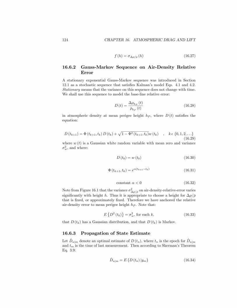
124 CHAPTER 16. ATMOSPHERIC DRAG AND LIFT
f (h) = ���=�� (h) (16.27)
16.6.2 Gauss-Markov Sequence on Air-Density RelativeError
A stationary exponential Gauss-Markov sequence was introduced in Section12.1 as a stochastic sequence that satis�es Kalman�s model Eqs. 4.1 and 4.2.Stationary means that the variance on this sequence does not change with time.We shall use this sequence to model the base-line relative error:
D (t) =��hP (t)
��hP (t)(16.28)
in atmospheric density at mean perigee height hP , where D (t) satis�es theequation:
D (tk+1) = � (tk+1; tk)D (tk) +p1� �2 (tk+1; tk)w (tk) ; k � f0; 1; 2; : : :g
(16.29)where w (t) is a Gaussian white random variable with mean zero and variance�2w, and where:
D (t0) = w (t0) (16.30)
� (tk+1; tk) = e�(tk+1�tk) (16.31)
constant � < 0 (16.32)
Note from Figure 16.1 that the variance �2��=�� on air-density-relative-error variessigni�cantly with height h. Thus it is appropriate to choose a height for ��=��that is �xed, or approximately �xed. Therefore we have anchored the relativeair-density error to mean perigee height hP . Note that:
E�D2 (tk)
= �2w, for each k, (16.33)
that D (tk) has a Gaussian distribution, and that D (tk) is Markov.
16.6.3 Propagation of State Estimate
Let Dnjm denote an optimal estimate of D (tn), where tn is the epoch for Dnjmand tm is the time of last measurement. Then according to Sherman�s TheoremEq. 3.9:
Dnjm = E fD (tn) jymg (16.34)

16.6. ATMOSPHERIC DENSITY ERRORS 125
Apply Eq. 16.34 to Eq. 16.29, where yk at time tk was the last measurementprocessed:
Dk+1jk = �(tk+1; tk) Dkjk (16.35)
Eq. 16.35 is the �lter state estimate propagation equation for the �lter time-update. Given measurement yk+1 at time tk+1 use Kalman�s �lter measurement-update theorem, derived from application of Eq. 16.34 to D (tk+1), for therepresentation:
Dk+1jk+1 = E fD (tk+1) jyk+1g (16.36)
Propagation of Dk+1jk+1 to time tk+2:
Dk+2jk+1 = �(tk+2; tk+1) Dk+1jk+1
16.6.4 State Estimate Error
De�ne the error in Dnjm by:
�Dnjm = Dn � Dnjm (16.37)
Insert Eqs. 16.35 and 16.29 into Eq. 16.37:
�Dk+1jk = �(tk+1; tk) �Dkjk +q1� �2k+1;kwk (16.38)
16.6.5 Process Noise Covariance
Base-Line Model
Square Eq. 16.38 and apply the expectation operator to get:
En��Dk+1jk
�2o= �2 (tk+1; tk)E
n��Dkjk
�2o+�1� �2k+1;k
��2w (16.39)
Notice that:
En��Dkjk
�2o< �2w (16.40)
due to the processing of measurements by the optimal �lter. Thus the stochasticsequence de�ned by Eq. 16.38 is not stationary. The second term in the right-hand side of Eq.16.39 is the base-line process noise covariance for deweightingprior estimates of D:
q��=�k+1;k =
�1� �2k+1;k
��2w (16.41)
For long propagation time intervals [tk; tk+1] the factor�1� �2k+1;k
�tends to
unity, and this adds �2w. For short propagation time intervals [tk; tk+1] the factor

126 CHAPTER 16. ATMOSPHERIC DRAG AND LIFT�1� �2k+1;k
�tends to zero, and only a small part of �2w is added. Thus the factor�
1� �2k+1;k�drives the variance E
n��Dk+1jk
�2otoward �2w in the absense of
measurements, but adds little or nothing during dense measurements. Whenmean values haP i and hF10i of aP and F10 are experienced, this is appropriatefor the base-line Gauss-Markov model.But for an active Sun (solar maximum) when aP and F10 are much larger
than haP i and hF10i, then an important model extension is called for. TheGauss-Markov model must be immediately interrupted to open the �lter gain,particularly during dense measurements.
Active Sun
The CIRA 1972 atmospheric density model �� is a function of several arguments.It will su¢ ce in this section to write:
�� = ���h; F10; �F10; aP ; tk+1
�(16.42)
De�ne the unitless ratio:
R =���hP ; F10; �F10; aP ; tk+1
��� (hP ; hF10i ; hF10i ; haP i ; tk+1)
(16.43)
and de�ne Rmax. Initialize:
Rmax = 1 (16.44)
Algorithm: If R > Rmax, set Rmax = R and de�ne:
Q��=�k+1;k = R2�2w (16.45)
else, set Rmax = R and de�ne:
Q��=�k+1;k = q
��=�k+1;k (16.46)
Use Q��=�k+1;k for air-density error process noise covariance deweighting. E¤ect:When �� is increasing at hP due to F10, �F10, and aP , then the air density varianceand �lter gain are immediately opened to enable tracking measurements toestimate signi�cant changes in air density. But when �� is decreasing at hP dueto F10, �F10, and aP , then the air density variance and �lter gain begin theirreturn to the baseline model.The active Sun model is an innovation in that it enables real time range
and/or Doppler spacecraft tracking measurements to estimate atmospheric den-sity corrections due to extreme solar activity (e.g., CME), or due to mean orquiet solar activity, in real time.

16.6. ATMOSPHERIC DENSITY ERRORS 127
Real-Time Filtering of Tracking Data
Near real time values of F10 and aP are derived from global observatory mea-surements. The 10 centimeter solar �ux measurement F10 is available once perday in near real time. The mean value �F10, averaged over the previous foursolar rotations, is also available once per day. The geomagnetic measurementaP , or KP , is available in near real time at the end of each three hour interval.Time propagations of F10 and aP provide values for real-time �ltering of
LEO tracking measurements. There is an obvious problem here. Namely, thepredicted values of F10 and aP always su¤er from propagation error. Typically,F10 and aP are treated as random walk stochastic sequences. Thus the lastobserved value is used as the predicted estimate. Consider the prediction errorin aP during the geomagnetic response to a commencement of coronal massejection at solar maximum. The aP may increase by several hundred per-centat any time during any three-hour prediction interval. Atmospheric density isextremely sensitive to sudden changes in aP . Since there exists no real-timemeasurement of aP , it is impossible to explicitly model the sudden change inatmospheric density in real-time. What can one do?If one forces the error variance on the relative atmospheric density parameter
to remain wide open during the entire time interval of solar maximum (sayfrom two to four years), then the �lter will be sensitive to sudden changes inatmospheric density due to range and/or Doppler tracking data. However, �lterorbit accuracy performance will su¤er during much of this time interval dueto passive geomagnetic activity and an excessively open gain on the relativeatmospheric density parameter. Also, the atmospheric density parameter willexperience huge and sudden estimate corrections, both positive and negative,while the �lter distributes its over-corrections throughout the multi-dimensionalstate space with time.If one controls the error variance on the relative atmospheric density pa-
rameter to behave in accordance with most variations in aP , then the �lterperformance will be relatively satisfactory and smooth most of the time. How-ever, the �lter will not be responsive to sudden changes in atmospheric density.
Initialization
For �lter initialization, de�ne:
Q��=�k+1;k = R2�2w (16.47)
The �lter should be restarted, using the �lter restart capability, following �lterinitialization.
16.6.6 Transform From Perigee Height to Current Height
Recall Eqs. 16.27 and 16.25 to write:

128 CHAPTER 16. ATMOSPHERIC DRAG AND LIFT
��� (h)
�� (h)= f (h)
f (hP )
f (hP )=
f (h)
f (hP )f (hP ) =
f (h)
f (hP )
��� (hP )
�� (hP )(16.48)
That is:
D (h) =f (h)
f (hP )D (hP ) (16.49)
Eq. 16.48 derives from:
�� (h)
�� (h)=
f (h)
f (hP )
�� (hP )
�� (hP )(16.50)
That is, square Eq. 16.50, apply expectation, and take square root to get Eq.16.48. From Eq. 16.26:
� (h) = �� (h) + �� (h)
= �� (h)
�1 +
�� (h)
�� (h)
�(16.51)
Insert Eq. 16.50 into Eq. 16.51:
� (h) = �� (h)
�1 +
f (h)
f (hP )
�� (hP )
�� (hP )
�and apply Sherman�s Theorem to get:
� (h) = �� (h)
�1 +
f (h)
f (hP )
�� (hP )
�� (hP )
�or:
� (h) = �� (h)
�1 +
f (h)
f (hP )D
�(16.52)
Eq. 16.52 de�nes the method to map the �lter estimate D at perigee height hPto the optimal estimate � (h) of atmospheric density, at current height h, for usein trajectory propagation.
16.6.7 Orbit Error Covariance
Acceleration Errors
Use the stochastic di¤erential operator � on Eq. 16.22 to relate random errorsin �zD to random errors in �, where both are serially correlated:
��zD = �1
2
�CDA
m
��s2��K (16.53)

16.6. ATMOSPHERIC DENSITY ERRORS 129
where �� is represented according to Eq. 16.50:
�� (h) = �� (h)f (h)
f (hP )
�� (hP )
�� (hP )= �� (h)
f (h)
f (hP )D (16.54)
Orbit Errors
Let Zi denote the 6x1 column matrix of position and velocity components, withepoch at ti. From the theory of Variation of Parameters in Universal Variables:
dZi
dt=@Zi
@ _z�zD
or:
dZi =@Zi
@ _z�zDdt
where @Zi=@�zD is a 6x3 matrix and �zD is a 3 � 1 matrix. Use the stochasticdi¤erential operator � on the equation above to relate random errors in Zi torandom errors in �zD, where both are serially correlated, and exchange di¤erentialoperators on the left-hand side:
d��Zi
�=@Zi
@ _z��zDdt
Use the de�nite integral operatorR tjtion the equation above to get:
�Zi =
Z tj
ti
@Zi
@ _z��zDdt
Apply the expectation operator E f�g to the outer product on the equationabove to get:
En��Zi
� ��Zi
�To=
Z tj
ti
Z tj
ti
�@Zi
@ _z(t)
�G (t; �)
�@Zi
@ _z(�)
�Tdtd� (16.55)
a 6� 6 matrix, where:
G (t; �) = E���zD (t)��z
TD (�)
(16.56)
a 3� 3 matrix, and it is assumed that:
E f��zDg = 0
E��Zi
= 0:
Repeat the above development using conditional expectations E��Zijy
and
En��Zi
� ��Zi
�T jyo where y is an m�1 column matrix of time-ordered mea-surements. Invoke Sherman�s Theorem to remove the optimal estimate �Zi:

130 CHAPTER 16. ATMOSPHERIC DRAG AND LIFT
�Zi = E��Zijy
so that:
E��Zijy
��Zi = 0
It is in this sense that the above assumptions are made. The optimal �lter will
always remove �Zi so that the orbit error covariance En��Zi
� ��Zi
�T jyo isalways calculated about �Zi, and not about the origin. Continue developmentwith the implicit agreement that all expectations are conditioned on measure-ments of y.Assume that the de�nite integral time jtj � tij < � is small. We will now
make what will seem to be rather gross approximations. They are justi�ed bythe fact that we are looking for at most only two digits of signi�cance in thecalculation of state error covariance quantities. First notice for Variation ofParameters in Universal Variables that approximately:
@Zi
@ _z�=�03�3I3�3
�Then: �
@Zi
@ _z(t)
�G (t; �)
�@Zi
@ _z(�)
�T�=�03�3 03�303�3 G (t; �)
�Eq. 16.55 becomes:
En��Zi
� ��Zi
�To �= Z tj
ti
Z tj
ti
�03�3 03�303�3 G (t; �)
�dtd�
Further, insert the double impulsive sifting integral into the integrand to get:
En��Zi
� ��Zi
�To=
�03�3 03�303�3 G (ti; ti) [tj � ti]2
�(16.57)
Insert Eqs. 16.53 and 16.54 into 16.56 to get:
G =
��12
�CDA
m
��s2�2
En(��)
2oKKT (16.58)
The orbit error transition function � will integrate the velocity error covari-ance G (ti; ti) [tj � ti]2 into position error covariance with a lag of one time unit[tj � ti]. A reasonable time increment upper bound is given by:
jtj � tij � � = P=50
where P is orbit period.

Chapter 17
Solar Photon Pressure
When spacecraft height is su¢ ciently low, the perturbative accelerations andmodeling errors due to solar photon pressure are masked by the perturbativeaccelerations and modeling errors due to air-drag. Knowledge of this height isnecessary for setting the force model for numerical trajectory propagation, andfor the estimation of drag and/or solar pressure parameters. Musen (see Baker[3] page 188) put this height at 800 km, whereas Vokrouhlicky [111] put thisheight at 300 km.Hujsak [39] presents a useful survey for identi�cation of state-of-the-art solar
pressure modeling.
17.1 Coordinate Frame for Solar Pressure
Stochastic stationary Gauss-Markov sequences are used for estimation of ob-servable solar pressure parameters. It is desireable to select a coordinate framethat best supports stationarity. The spacecraft-Sun line is a natural accessablechoice. To this end, let r denote the ECI position vector of the spacecraft centerof mass, let S denote the ECI position vector of the Sun center of mass, andlet � denote the vector from Sun center of mass to spacecraft center of mass.Then:
� = r� S (17.1)
enables de�nition of the unit vector s1 from Sun to spacecraft:
s1= �=� = [i]T
24 s11s12s13
35 (17.2)
where:
� =p� � � (17.3)
131

132 CHAPTER 17. SOLAR PHOTON PRESSURE
Use the orbit angular momentum de�ned in Section 1.2.1 to specify the unitvectorW. Then construct an intermediate vector T orthogonal to both s1 andW:
T =W � s1 (17.4)
and use its unit vector for the orthonormal basis:
s2 = T=T = [i]T
24 s21s22s23
35 (17.5)
where:
T =pT �T (17.6)
Finally:
s3 = s1 � s2 = [i]T24 s31s32s33
35 (17.7)
completes the orthonormal vector basis [s] for speci�cation of solar pressure:
[s] =
24 s1s2s3
35 (17.8)
The direction of solar photon motion is de�ned by s1. The rotation Rsi from [i]to [s] is given by:
[s] = Rsi [i] (17.9)
where:
Rsi =
24 s11 s12 s13s21 s22 s23s31 s32 s33
35 (17.10)
We also have need of unit vector U, de�ned in Section 1.2.1, to specify thedirection of IR photons from Earth to spacecraft.
17.2 Solar Pressure Acceleration
Pechenick�s model[94] is implemented for two approximations to the satelliteshape and characteristics. The di¤erence between the two models is simply amultiplicative scale factor which will be absorbed during the estimation process.The sphere with perfect absorption model is the model most commonly used intrajectory generation software.

17.2. SOLAR PRESSURE ACCELERATION 133
17.2.1 Notation
Symbols used for our solar pressure acceleration model are identi�ed in thefollowing table:
m mass of spacecraftL luminosity of Sun� distance from Sun to spacecraft�rS solar pressure acceleration of spacecraftrD di¤use re�ection coe¢ cientrS specular re�ection coe¢ cientn unit outward normal vector to spacecraft surface elementk unit vector de�nes direction of motion of photons from Sun to spacecraftdA in�nitesimal element of spacecraft surface areac speed of light
17.2.2 Conservation of Linear Momentum
From conservation of linear momentum, Pechenick[94] integrates over a convexilluminated spacecraft surface to �nd the following expression for spacecraftsolar pressure acceleration:
�rS =L
4��2mc
Z Z �(1� rS) k�
2
3rDn� 2rS
��k � n
�n
���k � n
�dA (17.11)
where:
k � n <0 (17.12)
k = s1 (17.13)
L = 3:8530� 1026 joulessec
�kg m2
sec3
�(17.14)
c = 2:99792458� 108 msec
(17.15)
1 au = 1:49600� 1011 m (17.16)
From Eq. 17.11 Pechenick derives the solar pressure acceleration for a sphericalsurface, a �at plate, a cylinder with closed ends, and various surface orientationaverages over the �at plate and cylinder.

134 CHAPTER 17. SOLAR PHOTON PRESSURE
17.2.3 Spherical Surface Di¤use Re�ection
Spacecraft solar pressure acceleration due to a spherical surface:
�rS =L
4��2mc�R2s
�1 +
4
9
�rDk (17.17)
where Rs is radius of the sphere. De�ne a constant:
KS =
�1 + 4
9
�L
4c,�default: 4:6411� 1017 kg-m
sec2
�(17.18)
This leaves rD, �, m, and Rs for use as time variables. Variations in � can beas large as twice the orbit semi-major axis if the orbit line of nodes lies alongthe Sun-spacecraft line. Then:
�rS = KS
�R2s�2m
�rDk (17.19)
Example: For a spherical spacecraft with � = 1 au, rD = 0:75, Rs = 1 m, andm = 1 kg we have:
j�rS j = 1:5553� 10�5msec2
Eq. 17.17 can be written in conventional operational form for di¤use photonre�ection:
�rS =L
4��2c
ASm
�1 +
4
9
�CRk (17.20)
where CR is the solar pressure coe¢ cient and AS is the spacecraft area exposedto the Sun:
CR = rD and AS = �R2s (17.21)
17.2.4 Spherical Surface Perfect Absorption
For perfect photon absorption:
�rS =L
4��2c
ASmCRk (17.22)
17.3 Eclipse Modeling
17.3.1 Selection
The cylindrical model used by GSFC/GTDS for solar pressure eclipsing is re-jected as a result of complete failure (10 sigma) of rigorous �lter-smoother con-sistency testing with real GEO tracking data.

17.3. ECLIPSE MODELING 135
Computational tractability currently excludes use of an atmospheric refrac-tion model for solar pressure eclipsing. For example, consider Vokrouhlicky�s[111] atmospheric refraction model. The angular width of a 50 km atmosphericslab, when seen from LAGEOS�height of 5500 km, is about 16 arcmin, and thisis half the apparent size of the undistorted solar disk. Due to di¤erential at-mospheric refraction of solar rays, the entire solar disk is easily contained withinthe 16 arcmin atmospheric width. The apparent solar image is highly �attened.The associated radiant force is highly correlated with this refraction e¤ect, andthe two-cone umbra-penumbra de�nition is made obsolete. Atmospheric refrac-tion produces a long-lived perturbation tail of solar rays deep into the umbraregion for the two-cone model.Until a tractable atmospheric refraction model is available, we shall use
Baker�s [3] two-cone eclipsing model with three sharply de�ned geometricalconditions: full sunlight, penumbra (partial eclipse), and umbra (total eclipse).Physically, the two-cone model is appropriate for a planet with no atmosphere.Baker�s model ignores atmospheric refraction and solar limb darkening.Rigorous �lter-smoother consistency testing with real GEO tracking data
demonstrated performance just within 3 sigmas. While poor, this result is farsuperior to that using a cylindrical eclipsing model. Also, the �lter-smoothertest result con�rms Vokrouhlicky�s analysis results relating to absence of modelsfor atmospheric refraction and solar limb darkening.
17.3.2 Baker�s Dual-Cone Eclipse Model
Baker [3] de�nes:
f ( ; �; �) =
8>><>>:1 � > + � full sunlight0 � + � � umbra, nonef1 � + � > penumbraf2 + � < � annular eclipse
(17.23)
where:
f1 = 1�"�
�
�2��� 1
2sin (2�)
�+
�� � 1
2sin (2�)
�#=� (17.24)
f2 =
�
�
�2(17.25)
sin = ae=r (17.26)
sin � = aS=� (17.27)
cos � = r � � (17.28)
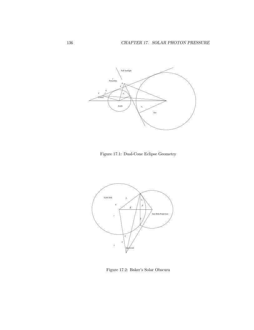
136 CHAPTER 17. SOLAR PHOTON PRESSURE
Sun
Earth
ae
aS
γ
η
ξ
Full Sunlight
Penumbra
Umbra
γ ξ
η
Figure 17.1: Dual-Cone Eclipse Geometry
Earth Disk
Sun Disk Projectionr
ae
~ρ
~aS
~R
α β
γ
η
ξ
Spacecraft
Figure 17.2: Baker�s Solar Obscura

17.4. STOCHASTIC SOLAR PRESSURE ERROR MODEL 137
sin� =2K
� (17.29)
sin� =2K
��(17.30)
cos� =�2 + 2 � �2
2� (17.31)
cos� =�2 � 2 + �2
2��(17.32)
S =� + + �
2(17.33)
K =pS (S � �) (S � ) (S � �) (17.34)
ae = 1 er ' r (17.35)
~aS = 108:966 er ' r� (17.36)
~R ' r� (17.37)
17.3.3 Earth Radius
The errors incurred by use of a two-cone model can be reduced by arti�cially in-�ating the modeled Earth radius so as to increase its shadow size. See Vokrouh-licky [111], midway through Section 5. Hujsak [39] cites McCarthy [70] and Link[62] on this practice, and notes that Link traces it back to 1707. McCarthy rec-ommends increasing the e¤ective radius of the Earth by 24 km to 6402 km, with1738 km for radius of the Moon, and 696000 km for radius of the Sun.
17.4 Stochastic Solar Pressure Error Model
Let p denote a unitless time-varying Gauss-Markov parameter for solar pressurede�ned by:
p = rD � �rD (17.38)
where rD is associated with Eq. 17.17, and �rD denotes a model constant withdefault value �rD = 0:75. Insert Eq. 17.38 into Eq. 17.19 to get:
�rS = KS
�R2s�2m
�(�rD + p (t)) k (17.39)

138 CHAPTER 17. SOLAR PHOTON PRESSURE
where p (t) is a stationary Gauss-Markov sequence:
p (tk+1) = � (tk+1; tk) p (tk) +p1� �2 (tk+1; tk)w (tk) ; k � f0; 1; 2; : : :g
(17.40)de�ned by Eqs. 16.29 (with D ! p) through 16.40, except that solar pressurevalues are assigned to �2! and �.

Chapter 18
GPS Solar Pressure Models
18.1 GSPM.04a
Implementation of the JPL GSPM.04a models for Block IIA and Block IIRsatellites follows Bar-Sever and Kuang (2004) [5]. This model was derived froma study of non-eclipsing satellites. The model is dependent on the angle of thesun out of the orbit plane (angle �), but holds the absolute value of the angle� at 14.5 degrees for cases where � goes below 14.5, as is the case for eclipsingsatellites. The form of the model is the same for Block IIA and Block IIRsatellites, but the coe¢ cients are di¤erent.
18.2 GSPM.04ae
Implementation of the JPL GSPM.04ae models for Block IIA and Block IIRsatellites follows reference Bar-Sever and Kuang (2005) [6]. This model wasderived as an extension of the GSPM.04a models Bar-Sever and Kuang (2004)[5], where the models deviate from the GSPM.04a models only for eclipsingsatellites. The model is dependent on the angle � of the sun out of the orbitplane, but drops one term involving division by the sine of � when � goes belowone degree. The form of the model is the same for Block IIA and Block IIRsatellites, but the coe¢ cients are di¤erent.
18.3 AeroT20
Implementation of the Aeropsace T20 model for use with Block IIA satellitesfollows O�Toole[90]. This model originally presented in Bar-Sever and Kuang(2004) [5].
139

140 CHAPTER 18. GPS SOLAR PRESSURE MODELS
18.4 AeroT30
Implementation of the Aeropsace T30 model for use with Block IIA satellitesfollows O�Toole[90]. This model originally presented in Fliegel [23].
18.5 Estimation
Consider estimation of the K1 and K2 parameters of the GPS solar pressuremodel. K1 is a unitless parameter which scales the acceleration along the sunto satellite line. The nominal value of K1 is 1:0. K2 is provided in unitsof 10�12m/s2 and speci�es the acceleration along the GPS body-�xed Y axis.This is often is referred to as the Y-bias acceleration. The Y axis points inopposite directions for Block IIA and Block IIR satellites when they are in theirnominal attitudes. Nominal values for K2 are on the order of 1. For estimationpurposes, the complete values of K1 and K2 are given as
K1 = �K1 +K1;GM (18.1)
K2 = �K2 +K2;GM (18.2)
where �K1 and are �K2 constant nominal values and K1;GM and K2;GM are se-quentially correlated Gauss-Markov random variables.

Chapter 19
Spacecraft Thrusting
The Frenét vector basis [f ] = (f1; f2; f3)T was selected for de�nition of coor-
dinate frame to represent input thrust accelerations. Many operational thrustmaneuvers are speci�ed to change only the orbit period (or semi-major axis)with thrusting along the spacecraft inertial velocity vector. The second vectorcomponent f2 of the Frenét basis isolates this e¤ect. See Eq. 1.13 through Eq.1.20 for complete de�nition of the Frenét vector basis.Impulsive maneuver models are physically unrealistic because the thrust
burn time interval is zero �in�nitely small. Physically realistic maneuver mod-eling imitates the maneuver with an appropriate �nite thrust burn time �for�nite maneuver.
19.1 Impulsive Maneuver Model
The impulsive acceleration model is always an approximation. It is a goodapproximation when the thrusting time interval is very short compared to orbitperiod. When the thrusting time interval is signi�cant compared to orbit period,the impulsive acceleration model is essentially useless.Model the impulsive acceleration as a three-dimensional vector Dirac delta
functional AD (t). Then in the three-dimensional velocity space we have a (dis-continuous) Heaviside step functional vector�V (t), and in the three-dimensionalposition space we have a (continuous) corner functional vector. �V (t) is a gen-eralized integral to AD (t).
19.1.1 Trajectory
De�ne components of vector �V = �V (t) with the equation:
�V = [i]T�V i = [f ]
T�V f (19.1)
where:
141

142 CHAPTER 19. SPACECRAFT THRUSTING
�V i =
24 �V i1�V i2�V i3
35 , inertial components (19.2)
�V f =
24 �V f1�V f2�V f3
35 , Frenét components (19.3)
Insert Eq. 1.20 into Eq. 19.1:
�V = [i]T�V i = [i]
TRTfi�V
f (19.4)
to get:
�V i = RTfi�Vf (19.5)
�V f = Rfi�Vi (19.6)
Eq. 19.5 enables conversion of input Frenét components of �V f to inertialcomponents of �V i. The inertial components of �V i = �V i (tC) are addeddirectly to velocity components of the predicted trajectory estimate at time ofcentroid tC .
19.1.2 Trajectory Error Covariance
Let us denote the error in vector �V with �V. Replace � with � in the notationabove to get:
�V i = RTfi�Vf (19.7)
�V f = Rfi�Vi (19.8)
Take the expectation of the outer product on Eq. 19.7:
En�V i
��V i
�To= RTfiE
n�V f
��V f
�ToRfi (19.9)
and give names to the 3� 3 covariance matrices:
P i�V = En�V i
��V i
�To(19.10)
P f�V = En�V f
��V f
�To(19.11)
Then:
P i�V = RTfiPf�VRfi (19.12)

19.1. IMPULSIVE MANEUVER MODEL 143
The user will specify the square-roots (sigmas) to the diagonal elements of theinput Frenét covariance matrix P f�V in user units, the program will convert tointernal units and square the user inputs to form variances, insert the variancesinto the diagonal elements of P f�V , and put zeros in the o¤-diagonal elementsof P f�V . The program will then evaluate Rfi and perform the multiplicationsindicated by Eq. 19.12 to calculate P i�V . The program will add P i�V = P i�V (tC)to the velocity covariance submatrix at time tC .
19.1.3 Time of Centroid tCLet tB and tE denote begin-burn and end-burn times, and let Af (t) denote aFrenét matrix 3 � 1 acceleration function across [tB ; tE ]. The time of centroidfor each Frenét component tCj is de�ned by:
tCj =Mfj
�V fj, j 2 f1; 2; 3g (19.13)
where:
Mfj =
Z tE
tB
tAfj (t) dt (19.14)
�V fj =
Z tE
tB
Afj (t) dt (19.15)
If the acceleration is given along Frenét component k only, where k 2 f1; 2; 3g,then:
tC = tCk (19.16)
If not, then a weighted combination of times is in order:
tC =3Xk=1
WktCk (19.17)
where:
3Xk=1
Wk = 1; Wk � 0 (19.18)
and where weight Wk, k 2 f1; 2; 3g, is derived from����V fj ��� ; j 2 f1; 2; 3g; e.g.:
Wk =
����V fk ���P3j=1
����V fj ��� (19.19)

144 CHAPTER 19. SPACECRAFT THRUSTING
Constant Acceleration Components
Given that Afj (t) is a time constant, then Eqs. 19.15, 19.14, and 19.13 arereduced to:
�V fj = Afj (tE � tB) (19.20)
Mfj =
1
2Afj�t2E � t2B
�(19.21)
tCj =1
2(tE + tB) (19.22)
19.2 Impulsive Maneuver Error Covariance
19.2.1 Notation
tk�1, time of last measurement before burn
tc, burn time centroid
tk = t(�)c = tc � �=2, start burn time
tk+1 = t(+)c = tc + �=2 = end burn time
tk+2 = time of �rst measurement after burn
P�Vc , cov for �V at tc
19.2.2 Time Relations
tk�1 < tk < tc < tk+1 < tk+2
� > 0

19.2. IMPULSIVE MANEUVER ERROR COVARIANCE 145
19.2.3 Covariance
Filter Running Forward with Time
Given Pk�1jk�1 at time of last measurement before burn, then:
P(�)cjk�1 = �c;k�1Pk�1jk�1�
Tc;k�1 + P
R Rc;k�1 (19.23)
P(+)cjk�1 = P
(�)cjk�1 + P
�Vc (19.24)
Pk+2jk�1 = �k+2;cP(+)cjk�1�
Tk+2;c + P
R Rk+2;c (19.25)
Smoother Running Backward with Time
Nominally:
~PLjL = PLjL (19.26)
...
~Pk+2jL = Pk+2jk+2 +Ak+2;k+3
h~Pk+3jL � Pk+3jk+2
iATk+2;k+3 (19.27)
The smoother covariance ~Pk+2jL is now available at time of �rst measurementafter burn. Then:
~P(+)cjL = P
(+)cjk�1 +Ac;k+2
h~Pk+2jL � Pk+2jk�1
iATc;k+2 (19.28)
where:
Ac;k+2 = P(+)cjk�1�
Tk+2;cP
�1k+2jk�1 (19.29)
and:
~P(�)cjL = P
(�)cjk�1 +Ac;c
h~P(+)cjL � P
(+)cjk�1
iATc;c (19.30)
where:
Ac;c = P(�)cjk�1
�P(+)cjk�1
��1(19.31)
146 CHAPTER 19. SPACECRAFT THRUSTING
19.3 Impulsive Maneuver Covariance
From the smoothed estimates ~Xk+1jL = ~X(+)cjL and ~XkjL = ~X
(�)cjL , the di¤erence
D ~XcjL = ~Xk+1jL� ~XkjL is calculated so as to quantify the di¤erence in smoothedestimates, before and after the impulsive maneuver. The purpose here is toderive the associated error covariance ~PcjL de�ned by:
~PcjL = E
��D ~XcjL
��D ~XcjL
�T�(19.32)
on the error di¤erence:
�D ~XcjL = � ~Xk+1jL � � ~XkjL (19.33)
So:
~PcjL = E
��� ~Xk+1jL � � ~XkjL
��� ~Xk+1jL � � ~XkjL
�T�
= E
�� ~Xk+1jL
�� ~Xk+1jL
�T�+ E
�� ~XkjL
�� ~XkjL
�T�
��E
�� ~Xk+1jL
�� ~XkjL
�T�+ E
�� ~XkjL
�� ~Xk+1jL
�T��(19.34)
Note that the sum in square brackets is symmetric, but neither of its terms is
symmetric. Covariance matrices E�� ~Xk+1jL
�� ~Xk+1jL
�T�and E
�� ~XkjL
�� ~XkjL
�T�are readily available from standard smoother output. But:
~Pk+1;kjL = E
�� ~Xk+1jL
�� ~XkjL
�T�(19.35)
and:
~Pk;k+1jL = E
�� ~XkjL
�� ~Xk+1jL
�T�(19.36)
are not available. Our purpose now is to derive a structure to evaluate ~Pk+1;kjLand ~Pk;k+1jL. Begin with Meditch[76], page 221, Eq. 6.48:
� ~XkjL = �Xkjk �Ak;k+1�~Xk+1jL � Xk+1jk
�(19.37)
where:
Ak;k+1 = Pkjk�Tk+1;kP
�1k+1jk (19.38)
Let Xk denote truth, and let Xkjj denote an estimate. The error �Xkjj in Xkjjis de�ned by:

19.3. IMPULSIVE MANEUVER COVARIANCE 147
�Xkjj = Xk �Xkjj (19.39)
Eq. 19.37 then becomes:
� ~XkjL = �Xkjk �Ak;k+1��Xk+1jk � � ~Xk+1jL
�(19.40)
Insert Eq. 19.40 twice into Eq. 19.36 to get:
~Pk;k+1jL = E
�� ~XkjL
�� ~Xk+1jL
�T�= E
��Xkjk
��Xk+1jk+1
�T�+Ak;k+1 [B � C] (Ak+1;k+2)T
+
�E
��Xkjk
�� ~Xk+2jL
�T�� E
��Xkjk
��Xk+2jk+1
�T��(Ak+1;k+2)
T
+Ak;k+1
�E
�� ~Xk+1jN
��Xk+1jk+1
�T�� �Xk+1jk+1
��Xk+2jk+1
�T�(19.41)
where:
B = E
��Xk+1jk
��Xk+2jk+1
�T�+ E
�� ~Xk+1jL
�� ~Xk+2jL
�T�(19.42)
C = E
�� ~Xk+1jL
��Xk+2jk+1
�T�+ E
��Xk+1jk
�� ~Xk+2jL
�T�(19.43)
19.3.1 Discussion
Eq. 19.41 appears to be recursive, containing both E�� ~XkjL
�� ~Xk+1jL
�T�and
E
�� ~Xk+1jL
�� ~Xk+2jL
�T�. If simpli�cation can be found to remove the implied
recursion, then implementation is feasible at a later date. If not, a conservativeapproximation to ~PcjL is given by:
~PcjL = E
�� ~Xk+1jL
�� ~Xk+1jL
�T�+ E
�� ~XkjL
�� ~XkjL
�T�where:
E
�� ~Xk+1jL
�� ~XkjL
�T�+ E
�� ~XkjL
�� ~Xk+1jL
�T�is ignored (set to zero). The recursion would need to be initialized from ini-tial conditions in the �lter and initial conditions in the smoother followed byassociated sequential calculations.

148 CHAPTER 19. SPACECRAFT THRUSTING
19.4 Finite Maneuver Model
19.4.1 Kinematics
b1
b2
b3
T
Φh ΦV 1
Figure 19.1: Unit Thrust Referred to Maneuver Frame
Let [t] = [t1; t2; t3]T denote an orthonormal vector basis variable [t] 2
f[i] ; [u] ; [f ]g that may be assigned inertial [i], Gaussian [u], or Frenét [f ] ac-cording to user selection. Thus [t] is a trajectory frame. Let [b] = [b1;b2;b3]
T
denote an orthonormal vector basis where b3 is de�ned to be the nominal thrustdirection. Thus [b] de�nes the nominal maneuver (thrust direction) coordinateframe. Relate [b] to [t] with the 3� 3 orthogonal rotation matrix Rbt:
[b] = Rbt [t] (19.44)
[t] = RTbt [b] (19.45)

19.4. FINITE MANEUVER MODEL 149
When Rbt = I3�3, then the nominal thrust direction b3 = t3 is referred directlyto a trajectory frame [t]. Let T = T (t) denote the time-dependent spacecraftthrust vector, and let T denote the thrust unit vector:
T = T=T (19.46)
where thrust magnitude T is de�ned:
T =pT �T (19.47)
Then T has components referred to [b]:
T = [b]T
24 T1T2T3
35 (19.48)
de�ned by horizontal angle 'h and vertical angle 'v such that:
tan'h =T1
T3(19.49)
tan'v =T2
T3(19.50)
T3 =�1 + tan2 'h + tan
2 'v��1=2
(19.51)
By inspection: �T1
�2+�T2
�2+�T3
�2= 1
19.4.2 Dynamics
Let us denote the acceleration vector due to thrust with AT . Then:
AT = AT T (19.52)
where AT is the acceleration magnitude. From Newton�s second law:
T = mAT (19.53)
where m is spacecraft mass.
19.4.3 Stochastic Sequences
Angles 'h and 'v, and relative thrust magnitude �T=T are modeled as Gauss-Markov biases, and are not expected to be large.

150 CHAPTER 19. SPACECRAFT THRUSTING
Estimate � Statesnone N/A noneT 'h; 'v;�T=T �T=TT 'h; 'v; T T'h; 'v; T 'h; 'v;�T=T 'h; 'v;�T=T'h; 'v; T 'h; 'v; T 'h; 'v; T'h; 'v; T T components T components
Table 19.1: Table Caption
19.4.4 Estimation
Thrust magnitude T , or relative thrust magnitude �T=T , angles 'h and 'v,and AT components on inertial, Gaussian, and Frenét frames may be estimated,with a variety of user selected options.

Part IV
Spacecraft Attitude
151


Chapter 20
Attitude Modeling
The attitude of satellites may be speci�ed through two mechanisms:
� Geometrically de�ned orientation of the body axes relative to speci�edinertial directions, referred to as the Aligned and Constrained attitudespeci�cation
� A time history of attitude states in the form of quaternions or Euler anglescontained in a �le
However the attitude for the satellite is de�ned, it is used in ODTK todetermine the location of antenna phase centers used in observation modeling.Antenna phase center locations are speci�ed as �xed locations in the body frameof the satellite. The origin of the satellite body frame is at the center of massof the satellite by default, but �xed coordinates in the body frame may alsobe speci�ed for the center of mass. The inertial location of the antenna phasecenter is computed for use in observation modeling as follows,
Rant= Rcm +M (rant � rcm) (20.1)
where Rcm is the inertial location of the center of mass of the satellite, M is thecurrent 3�3 rotation matrix from body �xed coordinates to inertial coordinates,rant is the antenna phase center location relative to the origin of the body frameexpressed in body �xed coordinates and rcm is the center of mass locationrelative to the origin of the body frame expressed in body �xed coordinates.
20.1 Antenna Phase Center Estimation
The GPS measurement models in ODTK support estimation of the antennaphase center location in the body frame of the satellite when applied to a spacebased GPS receiver. In this case, the antenna phase center coordinates areestimated as constants. Estimation of the antenna phase center is facilitated byapplying the chain rule to the observation partials with respect to the inertial
153

154 CHAPTER 20. ATTITUDE MODELING
antenna phase center location to obtain the observation partials with respect tothe antenna phase center location in the body �xed frame. If � is the observedquantity, then
@�
@rant=
@�
@Rant
@Rant
@rant=
@�
@RantM (20.2)

Part V
State Error Transition
155


Chapter 21
Transitive PartialDerivatives
21.1 State Error Transition Function
The stateX may contain one or more observable orbits Zi, associated observableacceleration model parameters Ai, associated observable measurement modelparameters Bi, and other observable parameters:
X =
26666666664
Z1
A1
B1
Z2
A2
B2
...
37777777775The state error transition function � (tk; tj) will be calculated as the Jacobianmatrix @X (tk) =@X (tj):
� (tk; tj) =@X (tk)
@X (tj)(21.1)
21.2 Position & Velocity Partials
Recall Eqs. 1.24, 1.25, and 1.35.
157

158 CHAPTER 21. TRANSITIVE PARTIAL DERIVATIVES
Z =
�z_z
�=
26666664z1z2z3_z1_z2_z3
37777775 =26666664Z1Z2Z3Z4Z5Z6
37777775for notation for spacecraft position component matrix z, velocity componentmatrix _z, and their composition Z. The 6x6 matrix of partial derivatives:
�Z (tk; tj) =@Z (tk)
@Z (tj)
moves position and velocity error �Z (t) from time tj to time tk:
�Z (tk) =@Z (tk)
@Z (tj)�Z (tj) = �
Z (tk; tj)�Z (tj)
21.2.1 Two-Body Transition Matrix
The two-body 6x6 matrix �ZTB (tk; tj) of two-body partial derivatives for Uni-versal Variables given by Herrick ([33] 15C)1 has been shown to be su¢ cient forgeocentric applications that have dense tracking data with time. But they havebeen shown to be insu¢ cient for sparce tracking data with time. They are alsolikely to be insu¢ cient for cases where two-body gravity is not the dominantforce acting on the spacecraft. For these cases it is appropriate to use variationalequations to incorporate perturbative e¤ects in the orbit transition function.
21.2.2 Variational Equations Transition Matrix
Eq. 21.10 gives the general structure for the di¤erential variational equations.
General Structure
Let �Z (tk; tj) denote the 6x6 matrix of variational equations. It is appropriateto �rst derive a representation for �Z (tk; tj). The time derivative _Z (t) of theorbit Z (t) is some nonlinear function f (Z; t) of the orbit Z and time t:
_Z (t) = f (Z; t) (21.2)
Recall Eq. 1.36:
Z (t) = 'z ft;Z (t0) ; t0; u (Z (�) ; �) ; t0 � � � tg (21.3)
Di¤erentiate Eq. 21.2 with respect to Z (t0) with t0 �xed
1A simple correction is required to the second equation of (Herrick 15C20B).

21.2. POSITION & VELOCITY PARTIALS 159
@ _Z (t)
@Z (t0)=@f (Z; t)
@Z
@'z@Z (t0)
=@ _Z (t)
@Z (t)
@Z (t)
@Z (t0)(21.4)
because Z (t0) is a constant. Then:
@ _Z (t)
@Z (t0)=
d
dt
@Z (t)
@Z (t0)(21.5)
Insert this into Eq. 21.4 to get:
d
dt
@Z (t)
@Z (t0)=@ _Z (t)
@Z (t)
@Z (t)
@Z (t0)(21.6)
Let us denote:
� (t) =@Z (t)
@Z (t0)(21.7)
A (t) =@ _Z (t)
@Z (t)(21.8)
and note that:
� (t) = I6�6 (21.9)
Eq. 21.6 has the form:
_� (t) = A (t) � (t) (21.10)
Symbolically, write the integral to Eq. 21.10 as:
� (t) = I6�6 +
Z t
t0
A (�) � (�) d� (21.11)
The implementation of Eq. 21.11 bene�ts from simultaneous numerical integra-tion with the numerical integration of the orbit.
The A Matrix
In essence, the problem for integration of the variational equation, Eq. 21.10,is to calculate the matrix A (t) de�ned by Eq. 21.8:
A =
�A11 A12A21 A22
�(21.12)
where:
A11 =@ _z
@z= 03�3 (21.13)
since position and velocity are instantaneously independent. Then:

160 CHAPTER 21. TRANSITIVE PARTIAL DERIVATIVES
A12 =@ _z
@ _z= I3�3 (21.14)
A21 =@�z
@z(21.15)
A22 =@�z
@ _z(21.16)
Geopotential
The geopotential is a function only of postion and time. Therefore A22 = 03�3,and we are left with the calculation only of A21.
Calculate A21
Write the geopotential function U (negative potential energy per unit spacecraftmass) as:
U =�
r
1Xn=0
�aer
�n nXm=0
Pnm (sin') fCnm cosm�+ Snm sinm�g
=1Xn=0
nXm=0
fCnmUnm + SnmVnmg (21.17)
where ' and � are geodetic latitude and longitude, Pnm (sin') are Legendrefunctions of degree n and order m, and:
Unm =
��anern+1
�Pnm (sin') cosm� (21.18)
Vnm =
��anern+1
�Pnm (sin') sinm� (21.19)
The 3�1 gravitational acceleration matrix �zeG, referred to an Earth-�xed ortho-normal vector basis, is derived from the 3�1 gradient vector component matrix5ethat has been applied to the geopotential function U :
�zeG = 5eU =1Xn=0
nXm=0
fCnm 5e Unm + Snm 5e Vnmg (21.20)
The gravitational acceleration matrix �zeG in Earth-�xed components is rotatedto an inertial component matrix �zG by application of the 3� 3 rotation matrix2Rie:
2Precession, nutation, Greenwich rotation, and polar motion.
21.3. AIR-DRAG PARTIALS 161
�zG = Rie�zeG = Rie
1Xn=0
nXm=0
fCnm 5e Unm + Snm 5e Vnmg (21.21)
Then the A21 matrix has the represention:
A21 =@�zG@z
= Rie
1Xn=0
nXm=0
�Cnm
@ (5eUnm)
@z+ Snm
@ (5eVnm)
@z
�(21.22)
Evaluation of the second derivative terms in Eq. 21.22 is accomplished with afast running recursive technique on indices n and m.
21.3 Air-Drag Partials
Consider:
X =
�ZD
�(21.23)
where Z is a 6x1 substate consisting of spacecraft position and velocity, and Dis a scalar 1x1 air-drag substate coe¢ cient. The drag parameter D is modeledas an exponential Gauss-Markov sequence. Then:
@X (tk+1)
@X (tk)=h
@X(tk+1)@Z(tk)
@X(tk+1)@D(tk)
i=
"@Z(tk+1)@Z(tk)
@Z(tk+1)@D(tk)
@D(tk+1)@Z(tk)
@D(tk+1)@D(tk)
#(21.24)
where:
@D (tk+1)
@Z (tk)= 01x6 (21.25)
The 6x6 position and velocity Jacobian matrix @Z (tk+1) =@Z (tk) is calculatedin the �lter TimeUpdate() function using either an analytic two-body approx-imation, a fully perturbative numerical method, or a fast running perturba-tive numerical method that uses Encke�s method. The 1x1 air-drag derivative@D (tk+1) =@D (tk) = � (tk+1; tk) is given by Eq. 16.31, and the 6x1 Jacobianmatrix @Z (tk+1) =@D (tk) is the subject of this section.Generalize Eq. 1.36 to get:
X (tk+1) = ' ftk+1;X (tk) ; tk; u (X (�) ; �) ; tk � � � tk+1g (21.26)
Insert Eq. 21.26 into the 6x1 Jacobian matrix expression @X (tk+1) =@D (tk) toget:

162 CHAPTER 21. TRANSITIVE PARTIAL DERIVATIVES
@X (tk+1)
@D (tk)=@' ftk+1;X (tk) ; tkg
@D (tk)=@'ntk+1; [Z (tk) ; D (tk)]
T; tk
o@D (tk)
(21.27)
The right-hand side of Eq. 21.27 can be equated to the de�nition of the partialderivative:
@'ntk+1; [Z (tk) ; D (tk)]
T; tk
o@D (tk)
=
lim�D!0
�1
�D
n'ntk+1; [Z (tk) ; D (tk) + �D]
T; tk
o� '
ntk+1; [Z (tk) ; D (tk)]
T; tk
oo�(21.28)
The second term on the right-hand side denotes the nominal propagation fromtk to tk+1, but the �rst term on the right-hand side requires an additionalpropagation from tk to tk+1 with the air-drag element modi�ed:
D (tk) �! D (tk) + �D (21.29)
Recall from the partial derivative de�nition that lim�D!0 f�g means that �D > 0is su¢ ciently small, and that �D 6= 0. Several values for �D should be tried in or-der to identify the linear region for �D; i.e., an interval where @X (tk+1) =@D (tk)has negligible variations. The 7x1 column matrix of partial derivatives @X (tk+1) =@D (tk)is thus calculated according to Eq. 21.28. These propagations are executed us-ing a fast running Encke propagator.
21.4 Solar Pressure Partials
Replace D with p in the discussion above.

Part VI
Ground LocationEstimation
163


165
The estimation of location in the Earth-�xed reference frame is supported bymany measurement models within ODTK. To obtain the observation partialswith respect to a terrestrial location in the Earth-�xed frame for estimationpurposes, the chain rule is applied to these observation partials with respect tothe inertial terrestrial location. If � is the observed quantity, then
@�
@RECF=
@�
@RECI
@RECI@RECF
=@�
@RECIM (21.30)
where M is the 3�3 ECF to ECI transformation matrix. There are two op-tions for ground location estimation: to estimate the 3D position of the groundlocation or to estimate only the latitude and longitude of the ground locationwhile the altitude remains �xed at a speci�ed value. In the second case, whereonly latitude and longitude are estimated an additional step must be taken totransform the partial derivatives with respect to Cartesian coordinates to par-tial derivatives with respect to geodetic coordinates. De�ne position as the 3 x1 matrix G:
G =
24 '�H
35 (21.31)
where ' is the geodetic latitude, � is the longitude and H is the altitude abovethe ellipsoid. Another application of the chain rule gives
@�
@G=
@�
@RECF
@RECF@G
(21.32)
The matrix �RECF
�G is computed using a spherical Earth approximation as
@RECF@G
=
24 �xECF �yECF xECF =R�yECF xECF yECF =R� 0 zECF =R
35 (21.33)
where
� =qx2ECF + y
2ECF (21.34)
� =�zECF
�(21.35)

166

Part VII
Measurements
167


Chapter 22
Tracking StationKinematics
22.1 Introduction
The purpose of this section is to derive and provide complete and consistentstation kinematics results. Tracking station kinematics are used several times,and at di¤erent places, in the ODTK orbit determination program. Appropriateresults include the calculation of:
� Unit range vector components on the ECEF frame from azimuth andelevation
� Azimuth and elevation from unit range vector components on the ECEFframe
� Rotation matrices for use in azimuth and elevation calculations
� Azimuth and elevation partial derivatives for use in the optimal �lter
� Station position vector components on the ECEF frame, given stationgeodetic latitude ', longitude �, and height h above ellipsoid (comparisonto known results enables validation)
� Station position vector components on the ECEF frame, given station geo-centric latitude '0, longitude �, and position vector length s (comparisonto known results enables validation)
� Rigorous transformations: From ('0; s) to ('; h) and from ('; h) to ('0; s)(comparison of transform to inverse transform �and to known results �enables validation)
� A table to show '-dependent di¤erences between '0 and ' for comparisonto white noise RMS on angles measurements (demonstrates necessity foroblate ellipsoid in IOD angles measurement models)
169

170 CHAPTER 22. TRACKING STATION KINEMATICS
Perhaps the most important result is the clarity provided in relating the var-ious coordinate frames required for use in IOD, the simulator, and the optimal�lter.
22.2 The Earth-Centered Unit Sphere
Let [i] denote the dextral orthonormal Earth centered inertial (ECI) vector basis,and let [e] denote the dextral orthonormal time-dependent Earth centered Earth�xed (ECEF) vector basis [e], where:
[i] =
24 i1i2i3
35 (22.1)
[e] =
24 e1e2e3
35 (22.2)
[e] = Rei [i] (22.3)
where e3 is coincident with the instantaneous polar axis of �gure, e2 and e3lie in the instantaneous equator of �gure, e1 lies in the Greenwich meridian of�gure, and e3 = e1 � e2. The 3 � 3 rotation matrix Rei is a product of fourrotations: precession, nutation, Greenwich rotation, and polar motion (PNGM).Let s denote an Earth centered ground station position vector with geo-
centric latitude angle '0 and East longitude angle �. Let [f ] denote the dextralorthonormal vector basis obtained from [e] by an East longitude � rotation fromthe Greenwich meridian to the station meridian:24 f1
f2f3
35 =24 cos� sin� 0� sin� cos� 00 0 1
3524 e1e2e3
35 (22.4)
That is:
[f ] = Rfe [e] (22.5)
where:
Rfe =
24 cos� sin� 0� sin� cos� 00 0 1
35 (22.6)
Note that the ground station position vector s and geocentric latitude angle '0
are contained in the meridian plane spanned by f1 and f3. The station vector sis de�ned by:
s = [f ]Tsf (22.7)

22.2. THE EARTH-CENTERED UNIT SPHERE 171
λ
φ'
s/s
e1
e2
e3=f3
f1
M3
Figure 22.1: Station Longitude Rotation
where:
sf =
24 s cos'0
0s sin'0
35 (22.8)
and where:
s =ps � s =
q(sf )
Tsf (22.9)
The station unit vector s is de�ned by:
s= s=s= [f ]Tsf (22.10)
where:
sf =
24 cos'0
0sin'0
35 (22.11)
De�ne the dextral orthonormal geocentric station vector basis:24 M1
M2
M3
35 =24 � sin'0 0 cos'0
0 �1 0cos'0 0 sin'0
3524 f1f2f3
35 (22.12)

172 CHAPTER 22. TRACKING STATION KINEMATICS
f1
f3
M3=s/s
M1
Φ’
Φ’
M2=f2
Figure 22.2: Geocentric Station Vector Basis
or:
[M] = RMf [f ] (22.13)
where:
RMf =
24 � sin'0 0 cos'0
0 �1 0cos'0 0 sin'0
35 (22.14)
22.3 Ellipse in Plane of f1 and f3Let p denote an Earth centered vector:
p = [f ]Tpf (22.15)
where:
pf =
24 pf1pf2pf3
35 (22.16)
that de�nes an Earth centered ellipse in the (f1; f3) plane with function:

22.3. ELLIPSE IN PLANE OF F1 AND F3 173
S�pf�= b2
�pf1
�2+ a2
�pf3
�2� a2b2 = 0 (22.17)
pf2 = 0 (22.18)
where a and b are semi-major axis and semi-minor axis respectively. Thus:
b2 = a2�1� e2
�(22.19)
where e denotes eccentricity of the ellipse. De�ne the �attening f with:
f =a� ba
(22.20)
Then:
e2 =a2 � b2a2
= 2f � f2 (22.21)
22.3.1 Normal Vector n�pf�
Di¤erentiate S�pf�with respect to pf to derive the gradient rf to the ellipse:
rf = [f ]T
24 @S=@pf10
@S=@pf3
35 = [f ]T24 2b2pf1
0
2a2pf3
35 (22.22)
De�ne the outward normal unit vector n to the ellipse:
n =rf=prf �rf (22.23)
Then:
n = [f ]T
266664�1� e2
�pf1=
r(1� e2)2
�pf1
�2+�pf3
�20
pf3=
r(1� e2)2
�pf1
�2+�pf3
�2377775 (22.24)
22.3.2 Geodetic Latitude
De�ne the geodetic latitude ' with its tangent function:
tan' =@S=@pf3
@S=@pf1=
pf3
(1� e2) pf1(22.25)
Compare to Eq. 22.17 to eliminate pf3 and solve for pf1 :
pf1 =a cos'p1� e2 sin2 '
(22.26)

174 CHAPTER 22. TRACKING STATION KINEMATICS
Back substitute to get:
pf3 =a�1� e2
�sin'p
1� e2 sin2 '(22.27)
De�ne:
N' =ap
1� e2 sin2 '(22.28)
Then:
pf =
24 pf1pf2pf3
35 =24 N' cos'
0N'�1� e2
�sin'
35 (22.29)
22.3.3 Normal Vector n (')
Insert Eqs. 22.26 and 22.27 into Eq. 22.24 to demonstrate:
n = [f ]Tnf (22.30)
where:
nf =
24 nf1nf2nf3
35 =24 cos'
0sin'
35 (22.31)
22.3.4 Station Height Above Ellipse
Let h denote the station height above the ellipse and measured along n. Then:
s = p+hn (22.32)
That is:
s = [f ]Tsf (22.33)
where:
sf =
24 (N' + h) cos'0��
1� e2�N' + h
�sin'
35 (22.34)

22.3. ELLIPSE IN PLANE OF F1 AND F3 175
f1
f3
φ
Rp
hn
s
Figure 22.3: Station Position Vector
22.3.5 R
De�ne:
R =Rn (22.35)
where:
R =pR �R = pf3= sin' = N'
�1� e2
�(22.36)
Thus:
R =R [f ]Tnf = [f ]
TRf (22.37)
where:
Rf =
24 Rf1Rf2Rf3
35 =24 N'
�1� e2
�cos'
0N'�1� e2
�sin'
35 (22.38)
22.3.6 Geocentric vs Geodetic Latitude
Fundamental Results
Compare Eq. 22.8 with Eq. 22.34 to write:
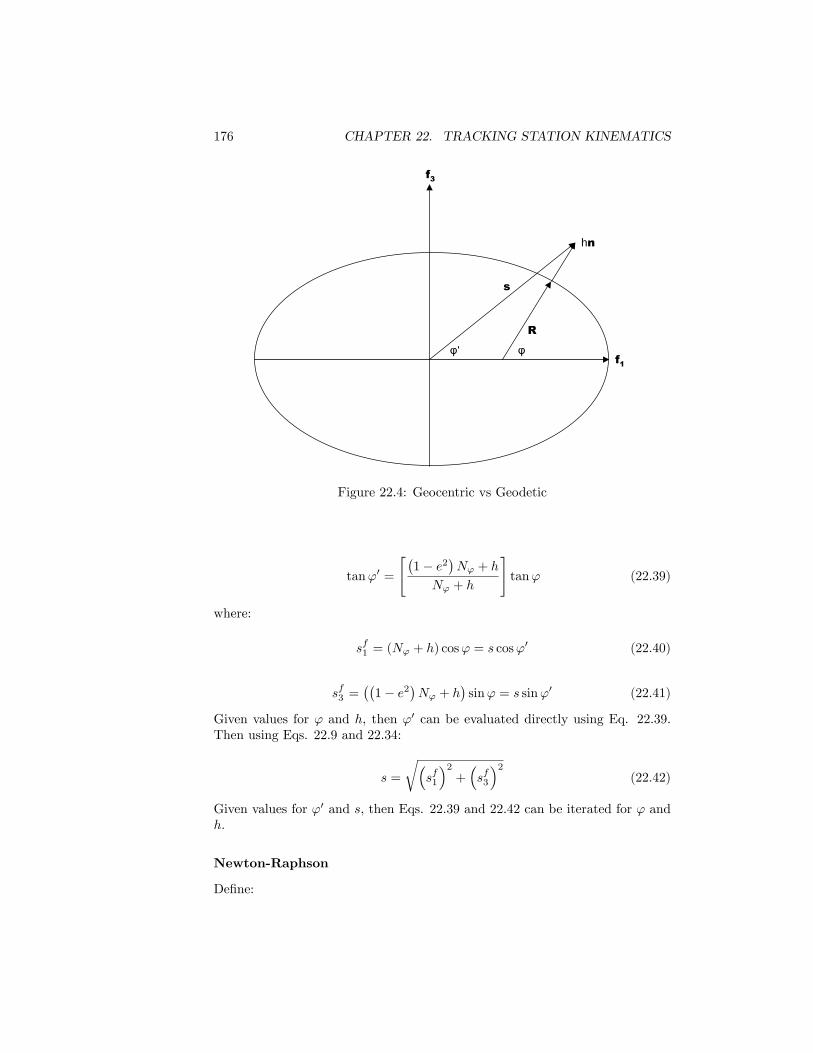
176 CHAPTER 22. TRACKING STATION KINEMATICS
f1
f3
φφ'
R
hn
s
Figure 22.4: Geocentric vs Geodetic
tan'0 =
"�1� e2
�N' + h
N' + h
#tan' (22.39)
where:
sf1 = (N' + h) cos' = s cos'0 (22.40)
sf3 =��1� e2
�N' + h
�sin' = s sin'0 (22.41)
Given values for ' and h, then '0 can be evaluated directly using Eq. 22.39.Then using Eqs. 22.9 and 22.34:
s =
r�sf1
�2+�sf3
�2(22.42)
Given values for '0 and s, then Eqs. 22.39 and 22.42 can be iterated for ' andh.
Newton-Raphson
De�ne:

22.3. ELLIPSE IN PLANE OF F1 AND F3 177
X =
�x1x2
�=
��'h
��(22.43)
f (X) =
�f1 (X)f2 (X)
�(22.44)
where:
f1 (X) = xyz � tan'0 = 0 (22.45)
f2 (X) =�sf1
�2+�sf3
�2� s2 = 0 (22.46)
x =�1� e2
�N' + h (22.47)
y = (N' + h)�1 (22.48)
z = tan' (22.49)
and sf1 and sf3 are de�ned by Eqs. 22.40 and 22.41.
Partial Derivatives@f (X)
@X=
"@f1@'
@f1@h
@f2@'
@f2@h
#(22.50)
where:
@f1@'
=@x
@'yz + x
�@y
@'z + y
@z
@'
�(22.51)
@f1@h
= z
�y +
@y
@h
�(22.52)
@f2@'
= 2:0
sf1@sf1@'
+ sf3@sf3@'
!(22.53)
@f2@h
= 2:0
sf1@sf1@h
+ sf3@sf3@h
!(22.54)
where:
@sf1@'
=@N'@'
cos'� (N' + h) sin' (22.55)
@sf1@h
= cos' (22.56)

178 CHAPTER 22. TRACKING STATION KINEMATICS
@sf3@'
=�1� e2
� @N'@'
sin'+ x cos' (22.57)
@sf3@h
= sin' (22.58)
@N'@'
=e2N' sin' cos'
1� e2 sin2 '(22.59)
@x
@'=�1� e2
� @N'@'
(22.60)
@x
@h= 1 (22.61)
@y
@'= �@N'
@'y2 (22.62)
@y
@h= �y2 (22.63)
@z
@'= sec2 ' (22.64)
@z
@h= 0 (22.65)
Algorithm
X(0) =
�'0
0
�(22.66)
X(k+1) = X(k) ��X(k), k 2 f0; 1; : : : ; ng (22.67)
�X(k) =
�@f (X)
@X
��1(k)
[f (X)](k) (22.68)
����X(n)��� < � (22.69)

22.3. ELLIPSE IN PLANE OF F1 AND F3 179
22.3.7 Topocentric Geodetic Vector Basis [N]
De�ne station zenith with N3:
N3= n = [f ]T
24 cos'0
sin'
35 (22.70)
Obtain a dextral orthonormal triad [N] with N1 as origin for station Northreference:
~N2 = n� f3 (22.71)
N2 = ~N2=
q~N2 � ~N2= [f ]
T
24 0�10
35 (22.72)
N1 = N2 �N3= [f ]T
24 � sin'0
cos'
35 (22.73)
f1
f3
N2=f2
N1
φ
φ
N3
Figure 22.5: Vector Basis for Angles Measurements
In matrix form we have:

180 CHAPTER 22. TRACKING STATION KINEMATICS
24 N1
N2
N3
35 =24 � sin' 0 cos'
0 �1 0cos' 0 sin'
3524 f1f2f3
35 (22.74)
That is:
[N] =RNf [f ] (22.75)
where:
RNf =
24 � sin' 0 cos'0 �1 0
cos' 0 sin'
35 (22.76)
This particular de�nition for rotation matrix RNf is necessary in order to si-multaneously: Put N3 at station zenith, de�ne station North origin with N1,and obtain a dextral orthonormal triad [N].
22.3.8 Topocentric Geocentric Vector Basis [M]
The rotation between geocentric latitude '0 and geodetic latitude ' is repre-sented by a rotation from vector basis [N] to vector basis [M] by angle � where:
� = '� '0 (22.77)
De�ne: 24 M1
M2
M3
35 =24 cos� 0 sin�
0 1 0� sin� 0 cos�
3524 N1
N2
N3
35 (22.78)
That is:
[M] =RMN [N] (22.79)
where:
RMN =
24 cos� 0 sin�0 1 0
� sin� 0 cos�
35 (22.80)
Check
Compare Eq. 22.79 with Eq. 22.13:
[N] = RNf [f ] (22.81)
where:
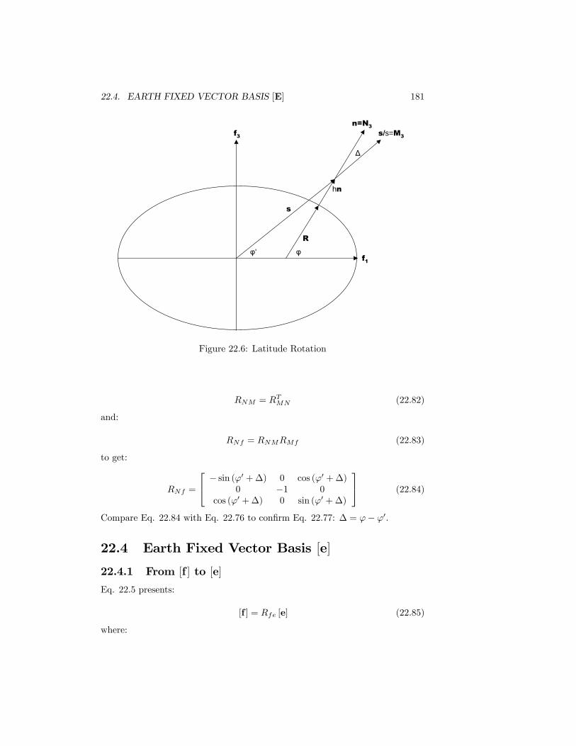
22.4. EARTH FIXED VECTOR BASIS [E] 181
f1
f3
φφ'
R
s
Δ
n=N3s/s=M3
hn
Figure 22.6: Latitude Rotation
RNM = RTMN (22.82)
and:
RNf = RNMRMf (22.83)
to get:
RNf =
24 � sin ('0 +�) 0 cos ('0 +�)0 �1 0
cos ('0 +�) 0 sin ('0 +�)
35 (22.84)
Compare Eq. 22.84 with Eq. 22.76 to con�rm Eq. 22.77: � = '� '0.
22.4 Earth Fixed Vector Basis [e]
22.4.1 From [f ] to [e]
Eq. 22.5 presents:
[f ] = Rfe [e] (22.85)
where:

182 CHAPTER 22. TRACKING STATION KINEMATICS
N3
M3=s/s
M1
N1
Δ
Δ
Figure 22.7: Latitude Di¤erence Rotation
Rfe =
24 cos� sin� 0� sin� cos� 00 0 1
35 (22.86)
Run the matrix transpose operator through Eq. 22.85 to get:
[f ]T= [e]
TRTfe = [e]
TRef (22.87)
where:
RTfe = Ref =
24 cos� � sin� 0sin� cos� 00 0 1
35 (22.88)
22.4.2 The Ellipsoid
Insert Eq. 22.87 into Eq. 22.15 to get:
p = [e]TRefp
f = [e]Tpe (22.89)
where:
pe = Refpf (22.90)

22.4. EARTH FIXED VECTOR BASIS [E] 183
Insert Eqs. 22.88 and 22.29 into Eq. 22.90 to get:
pe =
24 N' cos' cos�N' cos' sin�
N'�1� e2
�sin'
35 (22.91)
where pe � pe ('; �) speci�es each point on the Earth ellipsoid.
22.4.3 Station Vector
Insert Eqs. 22.87 into Eq. 22.33:
s = [e]TRefs
f = [e]Tse (22.92)
That is:
se = Refsf (22.93)
Geodetic: Given h and '
Insert Eq. 22.34 into Eq. 22.93:
se =
24 (N' + h) cos' cos�(N' + h) cos' sin���1� e2
�N' + h
�sin'
35 (22.94)
Geocentric: Given s and '0
Insert Eq. 22.8 into Eq. 22.93:
se =
24 s cos'0 cos�s cos'0 sin�s sin'0
35 (22.95)
22.4.4 Normal Vector n (')
Insert Eq. 22.87 into Eq. 22.30 to get:
n = [e]TRefn
f = [e]Tne (22.96)
where:
ne = Refnf =
24 cos' cos�cos' sin�sin'
35 (22.97)

184 CHAPTER 22. TRACKING STATION KINEMATICS
22.4.5 R
Insert Eq. 22.87 into Eq. 22.37:
R =R [f ]Tnf = [e]
TRefR
f = [e]TRe (22.98)
where:
Re = RefRf (22.99)
Thus:
Re =
24 Re1Re2Re3
35 =24 N'
�1� e2
�cos' cos�
N'�1� e2
�cos' sin�
N'�1� e2
�sin'
35 (22.100)

Chapter 23
Angles
23.1 Unit Range Vector
The instantaneous ground station unit range vector L is de�ned by:
L = �=� (23.1)
where:
� = r� s (23.2)
� =p� � � (23.3)
and where r is the Earth centered spacecraft position vector. The 3� 1 matrixLi of inertial components for L is de�ned by:
L = [i]TLi (23.4)
where:
Li =
24 Li1Li2Li3
35 (23.5)
23.2 Azimuth and Elevation
Let us denote azimuth and elevation with A and E, and de�ne:
� = 2� �A (23.6)
185

186 CHAPTER 23. ANGLES
N1
N2
N3
L
E
β H
1
Figure 23.1: Azimuth-Elevation Description
23.2.1 Construct L from Azimuth and Elevation
L is constructed here from an azimuth-elevation pair.
L = [N]TLN (23.7)
where:
LN =
24 LN1LN2LN3
35 =24 cosE cosA� cosE sinA
sinE
35 (23.8)
The following notational convention is used repeatedly in that which follows:Given any orthonormal rotation matrix R�� , then R�� = RT�� . Given the valuefor ', insert Eq. 22.75 into Eq. 23.7 to get:
L = [f ]TRfNL
N = [f ]TLf (23.9)
where:
Lf = RfNLN (23.10)
Into Eq. 23.9 insert Eq. 22.5 to get:
L = [e]TRefRfNL
N = [e]TLe (23.11)

23.2. AZIMUTH AND ELEVATION 187
where:
Le = RefRfNLN (23.12)
If Li is desired, insert Eq. 22.3 into Eq. 23.11:
L = [i]TRieRefRfNL
N= [i]TLi (23.13)
to get:
Li = RieRefRfNLN (23.14)
23.2.2 Construct Azimuth and Elevation from L
Given Li; construct an azimuth-elevation pair.
L = [i]TLi = [i]
TRieRefRfNL
N (23.15)
so:
LN = RNfRfeReiLi (23.16)
Solve Eq. 23.8 for A and E:
�AE
�=
24 tan�1��LN2 =LN1
�4QUADRANT
tan�1�LN3 =
q�LN1�2+�LN2�2�
35 (23.17)
23.2.3 Partial Derivatives of Azimuth and Elevation
Azimuth and Elevation with respect to LN
From Eq. 23.8:
sinA = �LN2 = cosE (23.18)
cosA = LN1 = cosE (23.19)
sinE = LN3 (23.20)
cosE =
q�LN1�2+�LN2�2
(23.21)
tanA = �LN2�LN1��1
(23.22)
tanE = LN3 = cosE (23.23)
Di¤erentiate Eqs. 23.22 and 23.23 to get the tensor covariant derivatives:

188 CHAPTER 23. ANGLES
@A
@LN=h
@A@LN1
@A@LN2
@A@LN3
i=�� sinA= cosE � cosA= cosE 0
�(23.24)
@E
@LN=h
@E@LN1
@E@LN2
@E@LN3
i=�� sinE cosA sinE sinA cosE
�(23.25)
Azimuth and Elevation with respect to Le
From:
LN = RNeLe (23.26)
derive:
@E
@Le=
@E
@LN@LN
@Le=
@E
@LNRNe (23.27)
@A
@Le=
@A
@LN@LN
@Le=
@A
@LNRNe (23.28)
Azimuth and Elevation with respect to Li
From
Le = ReiLi (23.29)
derive:
@E
@Li=
@E
@Le@Le
@Li=
@E
@LeRei (23.30)
@A
@Li=
@A
@Le@Le
@Li=
@A
@LeRei (23.31)
Azimuth and Elevation with respect to x
Let x denote the 3� 1 matrix of inertial components for the spacecraft positionvector. Then:
@E
@x=@E
@Li@Li
@x(23.32)
@A
@x=
@A
@Li@Li
@x(23.33)
It remains to �nd @Li=@x. From:
23.2. AZIMUTH AND ELEVATION 189
� =�L = r� s (23.34)
derive:
L =(r� s) ��1 (23.35)
Take the inner product of L with Eq. 23.35 to get:
� = L� (r� s) (23.36)
Convert the vectors in the last two equations to component arrays on the inertialframe:
Li =�x� si
���1 (23.37)
� =�Li�T �
x� si�
(23.38)
Insert Eq. 23.38 into Eq. 23.37 to get:
Li =�x� si
� ��Li�T �
x� si���1
(23.39)
Di¤erentiate with respect to x to get:
hI3�3 +
�x� si
� �x� si
�T=�2i @Li@x
=h(I3�3=�)�
�x� si
� �Li�T=�2i(23.40)
h�2I3�3 +
�x� si
� �x� si
�T i @Li@x
=h(�I3�3)�
�x� si
� �Li�T i
(23.41)
Multiply through by the inverse of the �rst factor to get the desired result:
@Li
@x=h�2I3�3 +
�x� si
� �x� si
�T i�1 h(�I3�3)�
�x� si
� �Li�T i
(23.42)
23.2.4 Construct Le from Azimuth and Elevation
Form LN with Eq. 23.8. Then from Eq. 23.12:
Le = RefRfNLN = ReNL
N (23.43)
where:
ReN =
24 � sin' cos� sin� cos' cos�� sin' sin� � cos� cos' sin�cos' 0 sin'
35 (23.44)

190 CHAPTER 23. ANGLES
23.2.5 Construct Azimuth and Elevation from Le
From Eq. 23.43:
LN = RNeLe (23.45)
where, using Eq. 23.44:
RNe = RTeN (23.46)
From Eq. 23.17:
�AE
�=
24 tan�1��LN2 =LN1
�4QUADRANT
tan�1�LN3 =
q�LN1�2+�LN2�2�
35 (23.47)
23.3 Direction Cosines
ODTK supports the processing of direction cosine observations. These obser-vations are referenced to a local dextral horizontal reference frame, the baselinedirections of which may rotated relative to the frame designated by N (North,West, Zenith) in the description of Azimuth and Elevation. The direction-cosinetriplet is de�ned by the components of L referred to the topocentric basis F.Analagous to our presentation of the topocentric basis for azimuth and elevationangles:
L = [F]TLF (23.48)
where:
LF =
24 LF1LF2LF3
35 (23.49)
The F basis is rotated about the F3 (or N3) axis by the amount ��� in theright-handed sense
RFN =
24 � cos(��) � sin(��) 0sin(��) � cos(��) 00 0 1
35 (23.50)
LF = RFNLN (23.51)
ODTK supports the processing of LF1 and LF2 as measurement types that origi-
nate from the Air Force Space Surveillance System (AFSSS) "Fence" (formerlyknown as the Naval Space Surveillance System, or NAVSPASUR). Only twodirection-cosine observations are needed in practice, since the third componentis mathematically related to the other two

23.3. DIRECTION COSINES 191
β
E'
L
F1N1
N2
F2
1
Δβ
Δβ
N3=F3
Figure 23.2: Direction Cosines Description
LF3 =
q�LF1�2+�LF2�2: (23.52)
Given the value for ', combine Eq. 22.75, Eq. 22.73 and Eq. 23.51 to get:
L = [F]TRFNL
N = [F]TLF (23.53)
Into Eq. 23.53 insert Eq. 22.5 to get:
L = [e]TRefRfNRNFL
F = [e]TLe (23.54)
where:
Le = RefRfNRNFLF (23.55)
If Li is desired, insert Eq. 22.3 into Eq. 23.54:
L = [i]TRieRefRfNRNFL
F= [i]TLi (23.56)
to get:
Li = RieRefRfNRNFLF (23.57)

192 CHAPTER 23. ANGLES
23.3.1 Construct Direction Cosines LF1 and LF2 from L
Given Li; construct a direction-cosine set given
L = [i]TLi = [i]
TRieRefRfNRNFL
F (23.58)
such that:
LF = RFNRNfRfeReiLi (23.59)
23.3.2 Partial Derivatives of Direction Cosines LF1 and LF2
LF1 and LF2 with respect to LN
From Eq. 23.51:
LF1 = � cos(��)LN1 � sin(��)LN2 (23.60)
LF2 = sin(��)LN1 � cos(��)LN2 (23.61)
LF3 = LN3 =
q�LN1�2+�LN2�2
(23.62)
Di¤erentiate Eqs. 23.60 and 23.61 to get the tensor-covariant derivatives:
@LF1@LN
=h
@LF2@LN1
@LF2@LN2
@LF2@LN3
i=�� cos(��) � sin(��) 0
�(23.63)
@LF2@LN
=h
@LF2@LN1
@LF2@LN2
@LF2@LN3
i=�sin(��) � cos(��) 0
�(23.64)
LF1 and LF2 with respect to Le
From:
LF = RFeLe (23.65)
derive:
@LF1@Le
=@LF1@LN
@LN
@Le=@LF1@LN
RNe (23.66)
@LF2@Le
=@LF2@LN
@LN
@Le=@LF2@LN
RNe (23.67)

23.4. X/Y ANGLES 193
LF1 and LF2 with respect to Li
From Eq. 23.65, derive:
@LF1@Li
=@LF1@Le
@Le
@Li=@LF1@Le
Rei (23.68)
@LF2@Li
=@LF2@Le
@Le
@Li=@LF2@Le
Rei (23.69)
LF1 and LF2 with respect to x
Let x denote the 3� 1 matrix of inertial components for the spacecraft positionvector. Then:
@LF1@x
=@LF1@Li
@Li
@x(23.70)
@LF1@x
=@LF1@Li
@Li
@x(23.71)
where @Li=@x is given by Eq. 23.42.
23.4 X/Y Angles
ODTK supports three types of X/Y angles, where the distinction between thetypes can be reduced to the unique de�nitions of the local reference frame inwhich the angles are measured. After a transformation to the correct localreference frame, theX/Y angle values and their partial derivatives are computedby a single set of formulas. We will describe the local reference frames viatheir relationship with the conventional topocentric frame (South, East, Zenith)which is related to the frame designated by N (North, West, Zenith) in thedescription of Azimuth and Elevation as
RTN =
24 �1 0 00 �1 00 0 1
35 (23.72)
�T = RTN�N (23.73)
23.4.1 X/Y East-West Reference Frame
The local reference frame for the computation of X/Y angles of the East-Westtype has basis vectors in the local East, North and Zenith directions. The localframe is related to the conventional topocentric frame as
RXT =
24 0 1 0�1 0 00 0 1
35 (23.74)

194 CHAPTER 23. ANGLES
�X = RXT �T (23.75)
23.4.2 X/Y North-South Reference Frame
The local reference frame for the computation ofX/Y angles of the North-Southtype has basis vectors in the local North, West and Zenith directions. The localframe is related to the conventional topocentric frame (South, East, Zenith) as
RXT =
24 �1 0 00 �1 00 0 1
35 (23.76)
�X = RXT �T (23.77)
23.4.3 X/Y Z Reference Frame
The local reference frame for the computation of X/Y angles with an accom-panying Z angle is related to the conventional topocentric frame (South, East,Zenith) as
RXT =
24 � cos(Z) � sin(Z) 0sin(Z) � cos(Z) 00 0 1
35 (23.78)
�X = RXT �T (23.79)
The Z angle speci�es a rotation about the Zenith direction in a right handedsense to specify the direction of the X axis where a rotation angle of zero corre-sponds to the X axis oriented with local North. X/Y angles of the North-Southtype are equivalent to X/Y Z angles with a Z angle of zero degrees. X/Y anglesof the East-West type are equivalent to X/Y Z angles with a Z angle of 270degrees.
23.4.4 X and Y Angles
The X angle is computed in the local frame as the angle from the Zenith direc-tion to the projection of the relative position vector into the Y-Z plane. The Xangle is de�ned to be positive for a rotation in a right handed sense about theX axis of the local frame.
X = tan�1���X2�X3
�(23.80)
The Y angle is measured in the local frame as the angle from the relativeposition vector to the projection of the relative position vector into the Y-Zplane. The Y angle is de�ned to be positive for a rotation in a right handedsense about the Y axis of the local frame.

23.5. GROUND BASED TRACKER 195
Y = tan�1
24 �X1q��X2�2+��X3�235 (23.81)
23.4.5 Partial Derivatives of X and Y Angles
The partial derivative of the X angle with respect to components of the relativeposition vector in the local frame is given by
@X
@�X=
�0
��X3(�X2 )
2+(�X3 )
2
��X2(�X2 )
2+(�X3 )
2
�(23.82)
The partial derivative of the Y angle with respect to components of the relativeposition vector in the local frame is given by
@Y
@�X=
" q(�X2 )
2+(�X3 )
2
�2��X1 �
X2
�2q(�X2 )
2+(�X3 )
2
��X1 �X3
�2q(�X2 )
2+(�X3 )
2
#(23.83)
23.5 Ground Based Tracker
Let us denote the right ascension and declination of L with �1 = � and �2 = �,referred to the inertial orthonormal vector basis [i]. Recall Eqs. 23.4 and 23.5to de�ne � and � with:
Li =
24 Li1Li2Li3
35 =24 cos � cos�cos � sin�sin �
35 (23.84)
from which:
� =
��1�2
�=
���
�=
24 tan�1�Li2=L
i1
�4�quadrant
tan�1�Li3=
q�Li1�2+�Li2�2�
35 (23.85)
23.5.1 Partials
We need a method to calculate the 2 � 3 matrix of partials @�=@z. Constructthe chain:
@�
@z=
@�
@Li@Li
@z(23.86)
Let us denote the 3� 1 matrix of ECI ground station position components withsi. Then recall Eqs. 1.24, 23.2, and 23.3 and to write:
�2 = zT z +�si�T �
si�� 2
�si�Tz (23.87)

196 CHAPTER 23. ANGLES
αδ
i1
i3
L
i2
Figure 23.3: Unit Range Vector Right Ascension & Declination
�Li = z � si (23.88)
Di¤erentiate the latter two equations with respect to z to get:
@�
@z=1
�
�z � si
�T(23.89)
@Li
@z=1
�
�I3�3 �
@�
@zLi�
(23.90)
Thus:
@Li
@z=1
�
�I3�3 �
1
�
�z � si
�TLi�
(23.91)
Use and di¤erentiate Eq. 23.84 with respect to Li:

23.6. SPACE BASED TRACKER 197
@�
@Li=
"@�@Li1
@�@Li2
@�@Li3
@�@Li1
@�@Li2
@�@Li3
#(23.92)
where:
@�
@Li1= � L2
L21 + L22
(23.93)
@�
@Li2=
L1L21 + L
22
(23.94)
@�
@Li3= 0 (23.95)
@�
@Li1= � L1L3p
L21 + L22
(23.96)
@�
@Li2= � L2L3p
L21 + L22
(23.97)
@�
@Li3=qL21 + L
22 (23.98)
The desired measurement partials are assembled with Eq. 23.86.
23.6 Space Based Tracker
Repeat the section above where vector s denotes space station position (notground station position).
23.7 Earth Ellipsoid Values
23.7.1 NIMA/NASA EGM96
(http://www.nima.mil/GandG/wgs-84/egm96.html)
a 6378137:0mf 1:0=298:2572235630� 0:3986004418� 1015m3=s2
!E 7292115:0� 10�11rad=s
Derived Values
f 3:3528106647474807� 10�3f2 1:124133935364444355382� 10�5e2 6:694379990141316996137� 10�3e 8:181919084262149433480� 10�2b2 40408299984661:445273030317b 6356752:314245179497563966

198 CHAPTER 23. ANGLES
23.7.2 On the EGM96 Ellipsoid
The white noise RMS on azimuth and elevation measurements for the AFSCFis about 0:03 deg. Compare this to the values in the third column to see thedisaster that would result from ignoring Earth�s oblateness in ODTK IOD,particularly in the neighborhood of ' = 45deg.
' (deg) '0 (deg) ('� '0) (deg) p (er)0 0.0 0.0 1.05 4.9666960870092 0.033303912990772 0.9999747429372310 9.9343942102791 0.065605789720866 0.9998997202669715 14.904067139653 0.095932860347192 0.9997771570449020 19.876629862375 0.12337013762532 0.9996106937301225 24.852912560483 0.14708743951726 0.9994052855179530 29.833635809829 0.16636419017093 0.9991670640335935 34.819388702350 0.18061129765039 0.9989031641467740 39.810610551928 0.18938944807156 0.9986215196130445 44.807576784018 0.19242321598195 0.9983306322619750 49.810389526291 0.18961047370932 0.9980393205002255 54.818973309214 0.18102669078556 0.9977564539217660 59.833076150493 0.16692384950734 0.9974906817456465 64.852276137025 0.14772386297540 0.9972501635449270 69.875993436424 0.12400656357643 0.9970423112018875 74.903507474004 0.096492525996069 0.9968735511399980 79.933978809966 0.066021190034306 0.9967491155814985 84.966475056686 0.033524943313807 0.9966728708250890 90.0 0.0 0.99664718933525

Chapter 24
Range
Range is time delay of a particular radio wave front from transmitter to re-ceiver. Let tT denote time of transmission, and tR denote time of receipt. Thenintrinsically, range (tR � tT ) has units of time. But typically and ideally, thetime delay is multiplied by the speed of light c in a vaccum to de�ne rangeRSR = c (tR � tT ) with units of distance.The radio wave front encounters high altitude clouds of electrons (ionosphere)
between transmitter and receiver. Each electron interacts with the wave frontwith an energy exchange in which the electron is displaced from its equilibriumposition and oscillates at its resonance frequency, and the radio wave front suf-fers a delay�tI . The size of�tI depends on the radio wave length, or frequency.At S-BAND (2 GHz) �tI is signi�cant. At Ku-BAND (18 GHz) �tI is rela-tively insigni�cant. When range measurements are generated at two distinctfrequencies the �rst order e¤ect of �tI can be easily removed. This is the casewith L-BAND GPS range measurements.If the transmitter and/or receiver is located at a ground station, then the
radio wave front encounters low altitude neutral tropospheric atoms and mole-cules (dominated by nitrogen and oxygen). The refracted wave front su¤erstropospheric refraction and a delay �tR. Tropospheric refraction is indepen-dent of carrier frequency but varies signi�cantly with elevation of antenna. Thecurrent version of ODTK uses the �RC [105] model developed for the AFSCN.When a transponder sits between transmitter and receiver there always ex-
ists a transponder time delay �tT . It is usually measured (with measurementerror) prior to use of the transponder, but varies as a function of its thermalenvironment.There are many other range delays (�tO = sum of other delays) with varying
degrees of signi�cance. Unmodelled cable lengths generate time delays. Varia-tions in the thermal and humidity environment of ground cables are responsiblefor variations in time delay. Antenna electromagnetic phase center varies asa function of geometry. Rotation between transmitter antenna and receiverantenna generates a time delay (Faraday rotation).Each of the two times tT and tR is de�ned by a clock (oscillator). If tT
199

200 CHAPTER 24. RANGE
and tR are de�ned by the same clock, the range measurements are said to becoherent. If tT and tR are de�ned by distinct clocks, the range measurementsare said to be non-coherent.
Two Clocks
Consider �rst the case for non-coherent range measurements; i.e., the case fortwo distinct clocks. There are two signi�cant and independent clock frequencye¤ects that must be modeled: relativity and clock phenomenology.
According to Albert Einstein, if these two clocks have di¤erent velocities withrespect to the same inertial frame, then they will tick at di¤erent frequencies(special relativity); clock frequency is a function of speed. And if they are atdi¤erent distances from the central body center of mass, then they will tickat di¤erent frequencies (general relativity); i.e., clock frequency is a function ofgravitational �eld. Both special and general relativity must be deterministicallymodeled.
When separate clocks are used for transmitter and receiver, it is usually thecase that one is inferior to the other. That is, the fractional frequency stabilityof one clock is superior. Then when the time tR of one clock is compared to thetime tT of the other to de�ne RSR, the frequency and phase errors of the inferiorclock are exposed. These random clock errors must be modeled by stochasticprocesses.
We associate the term one-way range measurement with two clocks.
One Clock
When the transmitter clock and receiver clock are the same clock, then thespeed and location of transmitter clock and receiver clock are the same. Thefrequency e¤ects due to special and general relativity vanish. Also, the trainof radio waves received are a mirror image of those emitted, so random clockfrequency and phase errors generated by the transmitter are subtracted out bythe receiver. Clock phenomenology vanishes. Coherent range measurements arethus relatively easy to model. We associate the term two-way range measure-ment with one clock.
There can be one or more transponders between the colocated transmitterand receiver. Transponders are placed on spacecraft and/or at ground locations(e.g., NASA TDRSS). Thus two-way range measurements may have two or morelegs with one or more transponders, but only one clock.
Range measurement time-tag is physically associated with the clock used tode�ne the time-tag. Possible candidates are tT and tR. Experience suggeststhat tR is preferred. Note that transponder times of receipt and emission arenot accessable by the transmitter/receiver clock.

24.1. CLASSICAL TWO-WAY RANGE 201
24.1 Classical Two-Way Range
Classical two-way range refers to use of a transmitter/receiver, and its clock,at a ground station, and a transponder on a spacecraft.. Time-node order forclassical two-way range: ti < tj < tp < tq.
24.1.1 Notation
c speed of light in vaccum
Uplink
ti time of radio wave emission from ground station radarsi ECI position vector of ground station radar at time titj time of radio wave receipt at spacecraft transponderrj ECI position vector of spacecraft at time tjRij range vector, function of ti and tjRij one-leg range from radar to spacecraftfUT radar transmitter frequency
Transponder Bias
�T transponder time bias
Downlink
tp time of radio wave emission from spacecraft transponderrp ECI position vector of spacecraft at time tptq time of radio wave receipt at ground station radarsq ECI position vector of ground station radar at time tqRpq range vector, function of tp and tqRpq one-leg range from spacecraft to radarfDT transponder transmitter frequency
24.1.2 De�nitions
Uplink
Rij = rj � si (24.1)
Note that range vector Rij points to node with latest time tj > ti.
Rij =pRij �Rij (24.2)
Rij = Rij=Rij (24.3)

202 CHAPTER 24. RANGE
Transponder
�T = tq � tp (24.4)
Downlink
Rpq = sq � rp (24.5)
Comparison of Eq. 24.5 with Eq. 24.1 idenit�es a convention in which therange vector always points to the node with latest time. Rpq points to node attime tq > tp. This convention produces symmetry in the one-way equations forrange-rate.
Rpq =pRpq �Rpq (24.6)
Rpq = Rpq=Rpq (24.7)
Two-Way
Riq = Rij + c�T +Rpq (24.8)
24.1.3 Special Relativity
Rij = c (tj � ti) (24.9)
Rpq = c (tq � tp) (24.10)
We now have two expressions for range Rij and two expressions for rangeRpq. Eq. 24.2 de�nes Rij geometrically in a �at cartesian space, and Eq. 24.9presents a derived result for Rij from special relativity theory. Similarly forRpq.
24.1.4 Calculation
Notice that the range vector Rij is not an instantaneous vector. Thus the rangeRij =
pRij �Rij is not invariant to rotation: One obtains di¤erent evaluations
in inertial and Earth �xed components. Second, spherical radio waves referred toan inertial frame are not spherical when transformed to an Earth �xed rotatingframe; i.e., the straight-line propagation of radio plane waves in an inertailframe transform to curved-line propagation in an Earth �xed rotating frame.Bottom line: Make life easy by performing all related evaluations using inertialvector components, and remember to independently rotate the station vectorfrom Earth-�xed to inertial components twice; i.e., at both transmit and receivetimes. This paragraph is dedicated to Dr Jim Woodburn.The simultaneous satisfaction of Eqs. 24.2 and 24.9 de�nes an uplink scalar
nonlinear problem that must be solved by iteration. Similarly for downlink.One of the four time-nodes for two-way range ti < tj < tp < tq is the given

24.2. SATELLITE TO SATELLITE TWO-WAY RANGE 203
two-way range time-tag tR. Begin calculation at the time-tag tR, and solve theproblem for uplink and downlink with the transponder bias inserted between.Example: If tR = tq (this is typical), solve the downlink problem �rst.In units of time, the relativistic two-way range representation is given by:
Rij=c+ �T +Rpq=c
In units of distance, the relativistic component of the range representation isgiven by:
RSR = Rij + c�T +Rpq (24.11)
at time-tag tR.
24.1.5 Complete Representation
Let us denote the complete two-way range measurement representation by R.Then:
R = RSR +RR +RI +RGM + wR (24.12)
where is RR is tropospheric refraction, RI is the ionospheric perturbation, RGMis a sequentially correlated Gauss-Markov random variable designed to accomo-date the sum of all other unmodeled range e¤ects, and wR is white Gaussianthermal noise. Parameter wR is not observable, and is not estimated. Theparameter RGM is observable, and is estimated by the sequential �lter.
24.2 Satellite to Satellite Two-Way Range
Satellite to satellite two-way range refers to use of a transmitter/receiver, and itsclock, on one spacecraft (the tracker), and a transponder on another spacecraft(the target). There is perfect symmetry between classical two-way ranging andsatellite to satellite two-way ranging. For the latter, the tracker spacecraft withthe transmitter/receiver and its clock is a moving "ground station", and thetarget spacecraft with the transponder is the spacecraft with the transponder.With this correspondence, the classical two-way ranging is directly applicableto satellite to satellite two-way ranging.
24.3 Bi-Static Range (One-Way)
Bi-static ranging refers to use of a transmitter/clock combination at a trans-mitting facility, a relay transponder on tracked spacecraft (the target), anda receiver/clock combination at a receiving facility. The bi-static range mea-surement is analgous to classical two-way ranging, except the transmitter andreceiver are not necessarily co-located, and the uplink path length may be sig-ni�cantly di¤erent than the downlink path. Each link path, or "leg", is treated
204 CHAPTER 24. RANGE
as a one-way ranging measurement, and the transponder delay is applied tothe downlink portion of the measurement. In the modeling of bi-static ranging,ODTK assumes that the transmitter clock and the receiver clock are completelysynchronized, and therefore does not account for stochastic clock errors in eitherthe uplink or downlink range measurements.

Chapter 25
Doppler
The Doppler measurement, de�ned by the receiver, is characterized by a phasecount Nhm on the Doppler frequency across a particular phase count time in-terval. Since the transmit frequency is known, the Doppler frequency can beextracted from the observed radio carrier frequency by di¤erencing the observedfrequency with the transmit frequency. Let th and tm denote the initial and �naltimes of the phase count time interval [th; tm], and de�ne �t = (tm � th). Thesetimes are de�ned by the receiver clock and the counting is performed by the re-ceiver. Intrinsically the Doppler measurement consists of an integer (integerphase count), plus a fraction, of accumulated phase, where each integer countis de�ned by a 2� excursion on phase. If the receiver presents the phase countNhm, the Doppler measurement has units of cycles. If the receiver presentsNhm=�t rather than Nhm, the Doppler measurement has units of cycles/time(mean frequency). If the receiver presents cNhm=fT , the Doppler measurementhas units of distance (range-di¤erence). If the receiver presents cNhm= (fT�t),the Doppler measurement has units of distance/time (mean range-rate).The Doppler measurement is perturbed by ionosphericTotal Electron Con-
tent (TEC) in the signal path. This e¤ect must be modeled.It is useful to think of the Doppler measurement in terms of its representation
as a range-di¤erence. If the range is perturbed by a particular physical e¤ect,then the range di¤erence over distinct times is perturbed accordingly. If aparticular physical e¤ect is a time-constant across light-time delay intervalswithin the phase count interval, then it will di¤erence to zero. But this isusually not the case.The Doppler measurement time-tag is physically associated with the clock
used to de�ne the phase count time interval. It is customary to place themeasurement time-tag at the time tm at end of the phase count time interval.Note that many sequential range values may be calculated within the phase
count time interval. When both range and Doppler measurements are derivedand presented by the receiver, it is customary to present only one range mea-surement with one Doppler measurement where both have the same time tag.
205

206 CHAPTER 25. DOPPLER
25.1 Classical Two-Way Doppler
25.1.1 Notation� wave length of radio carrier!D Doppler angular frequencyfD Doppler frequencyfO observed frequency
Uplink
_Rjij range-rate, due to relative motion between radar and spacecraft_tji frequency shiftnij number of wave lengths in uplink one-way signal path'ij total angular excursion by radio wave from radar to spacecraft
Downlink_Rqpq range-rate, due to relative motion between radar and spacecraft_tqp frequency shiftnpq number of wave lengths in downlink one-way signal path'pq total angular excursion by radio wave from spacecraft to radar
Two-Way
'iq total angular excursion by radio wave from radar to spacecraft to radar_Rqiq two-way range-rate, due to relative motion between radar and spacecraft�thm radio carrier phase count time intervalNhm phase count on Doppler frequency
25.1.2 De�nitions
fT = c=� (25.1)
!D = d'=dt (25.2)
fD = !D= (2�) (25.3)
Nhm =
Z tm
th
fDdtq (25.4)
�Rhm =
Z tm
th
dR = R (tm)�R (th) (25.5)
fO = fT + fD (25.6)

25.1. CLASSICAL TWO-WAY DOPPLER 207
Mhm =
Z tm
th
fOdtq (25.7)
�t = tm � th (25.8)
Uplink
_Rjij = dRij=dtj (25.9)
_tji = dti=dtj (25.10)
nij = Rij=� (25.11)
'ij = �2�nij (25.12)
Downlink
_Rqpq = dRpq=dtq (25.13)
_tqp = dtp=dtq (25.14)
npq = Rpq=� (25.15)
'pq = �2�npq (25.16)
Two-Way
niq = Riq=� (25.17)
'iq = �2�niq (25.18)
25.1.3 Expressions for Uplink Range-Rate
Di¤erentiate Eq. 24.1 with respect to time tj :
dRij
dtj=drjdtj
� dsidti
dtidtj
That is:
_Rjij = _rj � _si _tji (25.19)
Combine Eqs. 24.2 and 24.9 to write:

208 CHAPTER 25. DOPPLER
Rij =pRij �Rij = c (tj � ti) (25.20)
Di¤erentiate Eq. 25.20 with respect to time tj , and insert Eq. 25.19:
_Rjij = Rij ��_rj � _si _tji
�= c
�1� _tji
�(25.21)
Use the equation with second and third expressions from Eq. 25.21 to solve for_tji :
_tji =1� Rij � _rj=c1� Rij � _si=c
(25.22)
Use the equation with �rst and third expressions from Eq. 25.21 to calculate_Rjij :
_Rjij = c�1� _tji
�(25.23)
Solve Eq. 25.23 for the frequency shift _tji :
_tji = 1� _Rjij=c (25.24)
Alternate Expressions
Expand Eq. 25.22 to write:
_tji = 1� Rij � (_rj � _si)
c
!2641 + Rij � _sic
+
�Rij � _si
�2c2
+ � � �
375 (25.25)
and:
_Rjij =�Rij � (_rj � _si)
�2641 + Rij � _sic
+
�Rij � _si
�2c2
+ � � �
375 (25.26)
On comparison to Eq. 25.21, Eq. 25.26 provides a numerically stable methodfor evaluation of _Rjij .
25.1.4 Expressions for Downlink Range-Rate
Di¤erentiate Eq. 24.5 with respect to time tq:
dRpq
dtq=dsqdtq
� drpdtp
dtpdtq
That is:

25.1. CLASSICAL TWO-WAY DOPPLER 209
_Rqpq = _sq � _rp _tqp (25.27)
Combine Eqs. 24.6 and 24.10 to write:
Rpq =pRpq �Rpq = c (tq � tp) (25.28)
Di¤erentiate Eq. 25.28 with respect to time tq, and insert Eq. 25.27:
_Rqpq = Rpq ��_sq � _rp _tqp
�= c
�1� _tqp
�(25.29)
Use the equation with second and third expressions from Eq. 25.29 to solve for_tqp:
_tqp =1� Rpq � _sq=c1� Rpq � _rp=c
(25.30)
Use the equation with �rst and third expressions from Eq. 25.29 to calculate_Rqpq:
_Rqpq = c�1� _tqp
�(25.31)
Solve Eq. 25.31 for the frequency shift _tqp:
_tqp = 1� _Rqpq=c (25.32)
Alternate Expressions
Expand Eq. 25.30 to write:
_tqp = 1� Rpq � (_sq � _rp)
c
!2641 + Rpq � _rpc
+
�Rpq � _rp
�2c2
+ � � �
375 (25.33)
and:
_Rqpq =�Rpq � (_sq � _rp)
�2641 + Rpq � _rpc
+
�Rpq � _rp
�2c2
+ � � �
375 (25.34)
25.1.5 Two-Way Range-Rate
Recall Eq. 24.8:
Riq = Rij + c�T +Rpq
If the time-tag is at time tq, then di¤erentiate with respect to tq:

210 CHAPTER 25. DOPPLER
dRiqdtq
=dRijdtj
dtjdtp
dtpdtq
+ cd�Tdtq
+dRpqdtq
(25.35)
By de�nition:
�T = tq � tpso:
d�T = dtq � dtpSince the transponder bias �T is independent of Doppler frequency, we have:
d�T = 0
and this implies:
dtp = dtj
Then Eq. 25.35 reduces to:
dRiqdtq
=dRijdtq
+dRpqdtq
(25.36)
where:
dRijdtq
=dRijdtj
dtjdtp
dtpdtq
(25.37)
and:
dtjdtp
= 1 (25.38)
25.1.6 Two-Way Doppler Frequency Equation
Recall that 'iq is the total angular excursion by radio wave from radar tospacecraft to radar. Insert Eq. 25.17 into Eq. 25.18:
'iq = �2�Riq=� (25.39)
and then insert Eq. 25.1:
'iq = �2�fTRiq=c (25.40)
Di¤erentiate Eq. 25.40 with respect to time tq:
d'iqdtq
=�2�fTc
dRiqdtq
(25.41)
and use Eqs. 25.2 and 25.3 to get the two-way Doppler frequency equation:
fD = �fTc
dRiqdtq
(25.42)

25.1. CLASSICAL TWO-WAY DOPPLER 211
25.1.7 Two-Way Phase Count Equation
Take de�nite time integrals over both sides of Eq. 25.42 between th and tm:Z tm
th
fDdtq = �fTc
Z tm
th
dRiq (25.43)
and use the de�nition for Nhm to get the phase count equation:
Nhm = �fTc[Riq (tm)�Riq (th)] (25.44)
where Nhm is the two-way radio carrier phase count, fT is transmitter frequencyproduced by the ground station clock, Riq (th) is the two-way range at beginningof the phase count interval and Riq (tm) is the two-way range at the end of thephase count time interval [th; tm].The left hand quantity Nhm is produced only by receiver hardware. The
right-hand expression �fT�Rhm=c is used for the Doppler measurement repre-sentation in orbit determination algorithms. Eq. 25.44 relates receiver hardwareon the left to orbit determination software on the right.The radio wave propagation time interval [ti; tq] is typically very short com-
pared to the arbitrary phase count time interval [th; tm]. Check to see that boththe left-hand and right-hand sides of Eq. 25.44 have units of cycles; i.e., phasecount.Various forms of Eq. 25.44 are generated by manipulating fT and c. Then
the Doppler measurement will have di¤erent units. For all of these cases Nhmis produced by the receiver and �Rhm is used for the Doppler measurementrepresentation in orbit determination algorithms.Times tq do not exist continuously with real t. Thus the Riemann integrals
given in Eq. 25.43 should be replaced with discreet sums, Dirac-delta siftingintegrals, or appropriate Lebesgue integrals. The Riemann notation is symbolic.
25.1.8 Observed Frequency
Uplink at Spacecraft with Time tj
From de�nitions and Eq. 25.42 we have the frequency equation for fOj measuredby an observer in motion (e.g., a spacecraft) relative to the transmitter:
fOj = fT
�1� _Rjij=c
�(25.45)
where the factor�1� _Rjij=c
�is the uplink frequency shift.
Downlink at Radar with Time tq
If transponder performs no frequency shift, then:
fOq = fOj
�1� _Rqpq=c
�= fT
�1�
�_Rjij +
_Rqpq
�=c+ _Rjij
_Rqpq=c2�
(25.46)

212 CHAPTER 25. DOPPLER
25.1.9 Measurement Names
Receiver hardware engineers (e.g., Motorola) quite naturally refer to Nhm asa phase count measurement. DMA (NIMA) engineers have referred to phasecount measurements as Doppler measurements because the Doppler frequencyfD is integrated with time to produce phase count. Rearrange Eq. 25.44:
� c
fTNhm = �Rhm (25.47)
If the receiver produces values of �Nhmc=fT , it is easy to see why some en-gineers (NSWC) have referred to these measurements as delta-range measure-ments �Rhm. Divide this equation by �t = (tm � th):
� c
fT
Nhm�t
=�Rhm�t
(25.48)
and we have the same units as range-rate �Rhm=�t (AFSCF). But to model ameasurement derived from phase count as a range-rate is a big mistake, becausej�tj is never arbitrarily small. Divide Eq. 25.44 through by �t to get:
Nhm�t
= �fTc
�Rhm�t
(25.49)
If the receiver (e.g., NASA TDRSS) produces values of Nhm=�t, then the mea-surements have frequency units, and some engineers refer to them as frequencymeasurements.To summarize, we must address various transmitter/receiver hardware im-
plementations with various names, but with common physics. For all of thesecases Nhm is produced by the receiver and �Rhm is used for the Doppler mea-surement representation in orbit determination algorithms.
25.2 SCF ARTS Doppler
�Automated Remote Tracking Station�(ARTS) is used to identify any groundtracking station in the Air Force Satellite Control Facility (AFSCF).Multiply Eq. 25.44 through by �c= (fT (tm � th)) to get:
� c
fT
Nhm(tm � th)
=Riq (tm)�Riq (th)
(tm � th)(25.50)
where:
(tm � th) = 1 sec (25.51)
The left-hand side of Eq. 25.50 describes the Doppler measurement presented bythe ARTS receiver, and the right-hand side describes the Doppler representationto be used for orbit determination software. Riq (tm) and Riq (th) are both two-way ranges with uplink-downlink time nodes: ti < tj < tp < tq. The ARTS

25.2. SCF ARTS DOPPLER 213
Doppler measurement is inappropriately referred to as a range-rate measurementby ARTS documentation.Note that a value for c is required to solve for ranges Riq (tm) and Riq (th) by
orbit determination software. This raises the question as to whether the samevalue for c is used on both sides of Eq. 25.50.
25.2.1 Complete Representation
Let denote the complete two-way Doppler measurement representation. Then:
= SR + I + R + GM + w (25.52)
where SR is a function of spacecraft position and velocity, I is due to ionosphere, R is due to troposphere, GM is a sequentially correlated Gauss-Markov ran-dom variable designed to accomodate the sum of all other unmodeled Dopplere¤ects, and w is Gaussian white noise. Parameter w is not observable, andis not estimated. The parameter GM is observable, and is estimated by thesequential �lter.
25.2.2 Partial Derivatives
Position and Velocity
Recall Eq. 1.35, notation for spacecraft position and velocity:
Z =
�z_z
�=
26666664z1z2z3_z1_z2_z3
37777775 =26666664Z1Z2Z3Z4Z5Z6
37777775Let us denote the right-hand side of Eq. 25.50 with SR:
SR =Riq (tm)�Riq (th)
(tm � th)(25.53)
Di¤erentiate SR with respect to Z (tm), where tm = tq, to construct the 1x6matrix of partials:
@
@Z (tm)=
@ SR@Z (tm)
=1
(tm � th)
�@Riq (tm)
@Z (tm)� @Riq (th)
@Z (th)
@Z (th)
@Z (tm)
�(25.54)
remembering that the di¤erence (tm � th) is a time constant. The 6x6 orbittransition matrix:
�Z (th; tm) =@Z (th)
@Z (tm)

214 CHAPTER 25. DOPPLER
moves the denominator of the 1x6matrix @Riq (th) =@Z (th) from time th to timetm. Velocity partials emerge due to this transition matrix. Identify position andvelocity partials:
@Riq (t�)
@Z (t�)=
�@Riq (t�)
@z (t�);@Riq (t�)
@ _z (t�)
�; � in fh;mg (25.55)
Then:
@Riq (t�)
@z (t�)= (Lx; Ly; Lz) (25.56)
@Riq (t�)
@ _z (t�)= (0; 0; 0) (25.57)
using approximations:
Rpq (t�) = (Lx; Ly; Lz) [i] (25.58)
Doppler Bias
@
@� = 1 (25.59)
25.3 NASA STDN Doppler
25.3.1 Observed Range Rate
The NASA GSFC STDN document [102] de�nes the Observed Range Rate. TheDoppler measurement is the cumulative cycle count of 1000 times the Dopplerfrequency plus a 240-MHz bias frequency. It is time tagged at the time ofcycle counter reading. To process, convert Doppler data to decimal form. Theobserved average range rate is:
_R (T0) =�c
2fTKM
�N (T0)�N (T�1)
T0 � T�1� 2:4� 108
�(25.60)
where:c speed of lightfT transmit frequency in HertzK 240=221M 1000N cumulative Doppler-plus-bias counter readingT0; T�1 time of present and previous Doppler count, respectively

25.3. NASA STDN DOPPLER 215
25.3.2 Doppler Representation from the Observed RangeRate Equation
We shall attempt to derive an appropriate Doppler representation model equa-tion from the observed range-rate model Eq. 25.60 (and Teles�equation (4-2)[106]) in terms of the notation given previously herein. De�ne the S-BANDinput frequency fin with:
fin (t) = fD (t) + 240KHz (25.61)
where fD (t) denotes the Doppler frequency. De�ne the output Doppler countN (tm)�N (th) over [th; tm] with:
N (tm)�N (th) =Z tm
th
Jfin (t) dt (25.62)
where:
J = KM (25.63)
Then:
N (tm)�N (th) = J
�Z tm
th
fD (t) dt+ (240KHz) (tm � th)�
(25.64)
De�ne the average Doppler frequency �fD (tm) with:
�fD (tm) =
R tmth
fD (t) dt
tm � th(25.65)
and use Eq. 25.64 to get:
�fD (tm) =1
KM
�N (tm)�N (th)
tm � th� 2:40� 108
�Hz (25.66)
Multiply through both equations by �c= (2fT ) to get:
��c2fT
��fD (tm) =
��c2fT
� R tmth
fD (t) dt
tm � th
!=
��c
2fTKM
��N (tm)�N (th)
tm � th� 2:40� 108
�Hz
(25.67)Compare Eq. 25.67 with Eq. 25.60 to write:
_R (tm) =
��c2fT
� R tmth
fD (t) dt
tm � th
!(25.68)
Insert Eq. 25.43 to get:

216 CHAPTER 25. DOPPLER
_R (tm) =
�1
2
��Riq (tm)�Riq (th)
tm � th
�(25.69)
Eq. 25.69 is a one-way Doppler representation model due to the factor of 1=2.Since we model two-way range and Doppler internally as two-way measurementsour implementation of Eq.25.69 is given by:h
_R (tm)i2�way
=Riq (tm)�Riq (th)
tm � th(25.70)

Chapter 26
Troposphere
Our use of the term troposphere range refers to tropospheric propagation delayin distance units, or range error due to tropospheric refractivity. Troposphererange is one additive component of the complete one-way range measurementbetween a ground station and a spacecraft.
26.1 Troposphere Range
Let R denote troposphere range. Let " denote the geometric (non-refracted) ele-vation angle of an instantaneous range vector, referred to the local tangent plane,and let � denote the refracted elevation (apparent elevation). It is conventionalto indicate the dependence of troposphere range R on the geometric elevation": R � R ("). Current computational methods have two very di¤erent functionsin common: (i) A function to calculate the zenith troposphere range componentR (�=2), and (ii) A multiplicative mapping function m ("; "Z) = m ("; �=2) thatmaps the zenith troposphere range component R (�=2) to other elevations ".Thus:
R (") = m ("; �=2)R (�=2) (26.1)
26.1.1 Zenith Component
Physics
Refractivity N is related to index of refraction n with:
N = 10�6 (n� 1) (26.2)
For a spherically symmetric atmosphere, an integral expression for troposphererange R (�=2) at zenith1 has been presented (Mendes and Langley[82] Eq. (4)):
1Langley[58] also presents an integral expression for approximate troposphere range as afunction of non-zenith elevation.
217

218 CHAPTER 26. TROPOSPHERE
R (�=2) = 10�6Z rA
rS
Ndr (26.3)
where rS is the geocentric radius of the Earth�s surface and rA is the geocentricradius of top of the neutral atmosphere.
Crane Model (not implemented in ODTK)
The classic model for radio refractivity of the neutral troposphere was de�nedby Crane ([14]1976):
N = k1pdT+ k2
pwT+ k3
pwT 2
(26.4)
where pd (mb) and pw (mb) are partial pressures of dry gases and water vapor,T is absolute temperature (K), and:
k1 77:6� 0:1K=mbk2 72:0� 9:0K=mbk3 (3:75� 0:03)� 105K2=mb
(26.5)
Values for pd (mb) and pw (mb) are derived from measurements of temperature,pressure, and relative humidity. See below.
Thayer/Owens Improvement (not implemented in ODTK)
Crane�s model was improved by Thayer ([107]19742) to account for non-idealgaseous behavior of the atmosphere:
N = k1pdTZ�1d + k2
pwTZ�1w + k3
pwT 2Z�1w (26.6)
where Z�1d and Z�1w are inverse compressibility factors for dry air and watervapor. Expressions for them are given by Owens ([91]19673):
Z�1d = 1:0 + 10�4pd
�57:90� 10�4
�1:0 +
0:52
T
�� 9:4611 t
T 2
�(26.7)
Z�1w = 1:0 + 1650:0� 10�5 pwT 3�1:0� 104 � 1317:0t+ 17:5t2 + 0:144t3
�(26.8)
where T and t are temperatures in units Kelvin and Celsius. Constants for Eq.26.6:
k1 77:6036� 0:014K=mbk2 64:8000� 0:080K=mbk3 (3:7760� 0:004)� 105K2=mb
(26.9)
2Thayer�s extension seems to predate Crane. The Crane date was given by Ifadis withoutreference, and Ifadis implies that Thayer�s extension is an improvement over Crane. Langley�sbibliography[58] con�rms the two dates.
3 Indeed!?

26.1. TROPOSPHERE RANGE 219
Davis Modi�cation
A more compact form for Eq. 26.6 was presented by Davis, et. al. ([16]1985):
N = k1Rd�+ k0
2
pwTZ�1w + k3
pwT 2Z�1w (26.10)
using equation of state:
pi = Zi�iRiT (26.11)
where pi is the partial pressure of an atmospheric constutuent, �i is the massdensity, and Ri the speci�c gas constant for that constituent. So Rd is thespeci�c gas constant for dry air, and k
0
2 = (17� 10)K=mb.Davis also presents the form of the hydrostatic delay based on Saastemoinen,
Rh =h(0:0022768� 0:0000005) m
mbar
i P0f (�;H)
(26.12)
where
f (�;H) = 1� 0:00266 cos (2�)� 0:00028H (26.13)
In the above, � is the geodetic latitude and H is the height in kilometers abovethe geoid of the reference point. This is the a priori zenith delay model used inthe Saastemoinen model in ODTK.
Refractivity Partition
Refractivity is presented as the sum of hydrostatic and wet components:
N = Nh +Nw (26.14)
where:
Nh = k1Rd� (26.15)
Nw =�k2pwT+ k3
pwT 2
�Z�1w (26.16)
Tropospheric Range Partition
Tropospheric range has the form:
R = Rh +Rw (26.17)
where:
Rh = 10�6Z rA
rS
Nhds (26.18)
Rw = 10�6Z rA
rS
Nwds (26.19)

220 CHAPTER 26. TROPOSPHERE
26.1.2 Mapping Function
All mapping functions tested by Mendes and Langley[82] demonstrated sub-centimeter accuracy for elevation angles above 15 degrees. For elevation anglesbelow 10 degrees, only a select few were found to adequately meet the require-ments imposed by space geodetic techniques. Functions by Herring, Ifadis, andNiel were recommended as best performing, especially for lower elevations. Leastsatisfactory performance was associated with Hop�eld-based functions and theMarini-Murray function.Marini ([68]1971) de�ned a continued fraction on sin (") to model the map-
ping function m ("):
m (") =1
sin (") +a
sin (") +b
sin (") + c
(26.20)
and an illustrative numerical example is presented. Marini�s mapping functionwas adopted and modi�ed by several investigators. In common, each model hasthree parameter functions a, b, and c, but they are de�ned di¤erently by eachinvestigator.
IFADIS-GLOBAL (Ifadis) (not implemented in ODTK)
Marini�s[68] model structure of the mapping function m (") was adopted byIfadis ([44]1986):
m (") =1
sin (") +a
sin (") +b
sin (") + c
(26.21)
where:
a = k1 + k2 (P0 � 1000) + k3 (T0 � 15) + k4ppw (26.22)
b = k1 + k2 (P0 � 1000) + k3 (T0 � 15) + k4ppw (26.23)
Note: One of the repeated equations above is surely in error.
c = 0:078 (26.24)
MTT (Herring) (not implemented in ODTK)
Marini�s[68] model of the mapping function m (�) was modi�ed by Herring([34]1992) to arrive at the form:

26.1. TROPOSPHERE RANGE 221
m (") =
1 +a
1 +b
1 + c
sin (") +a
sin (") +b
sin (") + c
(26.25)
where[43]:
a = [1:2320 + 0:0130 cos'� 0:0209H� + 0:00215 (Ts � 10)] 10�3 (26.26)
b = [3:1612� 0:1600 cos'� 0:0331Hs + 0:00206 (Ts � 10)] 10�3 (26.27)
c = [71:244� 4:293 cos'� 0:149Hs � 0:0021 (Ts � 10)] 10�3 (26.28)
NMF Niell
Niell (26.301993) extended the Herring formula with a height correction term:
m (") =
1 +a
1 +b
1 + c
sin (") +a
sin (") +b
sin (") + c
+ 10�3HsMh (26.29)
where:
Mh =1
sin "�
1 +aht
1 +bht
1 + cht
sin (") +aht
sin (") +bht
sin (") + cht
(26.30)
and aht, bht, and cht are constants. See Niell ([89]2002) for his recent model ofmapping functions.The parameters (a, b, c) of the hydrostatic mapping function all have the
form
� (�; t) = �avg (�)� �amp (�) cos�2�
t� T0365:25
�(26.31)
where �avg (�) and �amp (�) are computed based on interpolation of tabulatedvalues as a function of geodetic latitude (�), t is the time in days past the

222 CHAPTER 26. TROPOSPHERE
beginning of the year and T0 is a phase of 28 days. The parameters (a, b, c)of the wet mapping function are simply constants which are interpolated fromtabulated values as a function of geodetic latitude. These are the mappingfunctions used with the Saastemoinen model in ODTK. The combination of theSaastemoinen a priori hydrostatic zenith model with the Niell NMF mappingfunction is also the recommended by McCarthey and Petit [71].
Marini Murray
The Marini Murray model is commonly used in satellite laser ranging applica-tions. It is not separated into hydrostatic and wet component, but takes theform
R =f (�)
f (';H)
A+B
sinE + B=(A+B)sinE+0:01
(26.32)
The site location function is given by
f (';H) = 1� 0:00266 cos (2')� 0:00031H (26.33)
where ' is the geodetic latitude and H is the height in kilometers above thegeoid of the reference point. The laser frequency parameter is given by
f (�) = 0:9650 +0:0164
�2+0:000228
�4(26.34)
where � is the laser wavelength in micrometers. A and B are computed as
A = 0:002357P0 + 0:000141e0 (26.35)
B =�1:084� 10�8
�P0T0K +
�4:734� 10�8
� �P 20T0
� �2
3� 1=K
�(26.36)
where,
e0 =
�(relative humidity (%))
100
�eSfW (26.37)
eS = 0:01 exp�1:2378847� 10�5T 20 � 1:9121316� 10�2T0 + 33:93711047� 6:3431645� 103T�10
�(26.38)
fW = 1:00062 + 3:14� 10�6P0 + 5:6� 10�7 (T0 � 273:15)2 (26.39)
K = 1:163� 0:00968 cos (2')� 0:00104T0 + 0:00001435P0 (26.40)

26.2. PARTIAL PRESSURE MEASUREMENTS 223
and T0 is the temperature in degrees Kelvin, P0 is the pressure in millibars and(relative humidity (%)) is the relative humidity expressed as a percentage. Theuse of this model with laser ranging data is the recommended by McCartheyand Petit [71].
Estimation Estimation of corrections to the troposphere corrections is doneestimating corrections to the zenith delay of the wet component. The hydro-static portion of the troposphere correction is assumed to be perfectly accurate.The contribution of the wet component is initially zero. The partial of the tro-posphere range correction with respect to the troposphere estimate is thereforegiven by the wet mapping function.
26.2 Partial Pressure Measurements
A partial pressure is the pressure that would be exerted by one component ofa mixture of gases if it were present alone. The total atmospheric pressure isthe sum of all partial pressures. Partial pressure values are derived from in-situmeasurements of atmospheric pressure, temperature, and relative humidity. Thepartial pressure pd for dry gases is approximated with the measured total ambi-ent pressure. The partial pressure pw for water vapor is temperature dependent;e.g., pw = 32mb for T = 25degC (tropics), and pw = 1:2mb for T = �20 degC(polar vortex). Its value is derived from a measurement of relative humidity(RH):
pw =�p0w�(RH)
where p0w is the partial pressure of water vapor at saturation, derived from atemperature dependent table. And RH, for constant water vapor, is tempera-ture dependent: If the amount of water vapor is held constant, then increasingtemperature decreases RH, and decreasing temperature increases RH. If tem-perature is held constant, then adding water vapor increases RH, and removingwater vapor decreases RH.The dew-point is the temperature to which the air would have to be cooled,
without changing pressure or moisture content, to reach saturation.The psycrometer and chilled-mirror hygrometer (dew-point meter) are stan-
dard sensors for measurements of humidity. A carbon resistance hygrometerand a human-hair hygrometer have also been developed to measure humidity.The psycrometer consists of two thermometers, a dry-bulb thermometer and
a wet-bulb thermometer, and tables of associated data. The wet-bulb ther-mometer measures the temperature to which objects are cooled by evaporationof water. The temperature di¤erence between dry-bulb and wet-bulb thermome-ters is indexed to the dry-bulb temperature in a standard table to derive a valueof RH.The chilled-mirror hygrometer is a temperature controlled mirror in which
the mirror is cooled until condensation occurs. The condensation temperature

224 CHAPTER 26. TROPOSPHERE
is the dew point measurement. The dew point is directly related to the amountof moisture in the air, so is an excellent indicator of absolute humidity.The carbon resistance hygrometer derives from the observation that as hu-
midity increases, water molecules �ll up pores in a carbon resistor; i.e., resistancein carbon is inversely proportional to relative humidity.The human-hair hygrometer derives from the fact that human hair lengthens
as relative humidity increases.
26.3 Atmospheric Thermodynamics
26.3.1 State Variables
Pressure
Atmospheric pressure p is the weight of the atmosphere per unit area. Averagesea level pressure:
1atm = 1013:25mb = 14:7psi = 29:92"Hg
Temperature
Let T denote temperature, and let K, C, and F denote units in Kelvin, Centi-grade, and Fahrenheit. Temperature is directly proportional to kinetic energyof a molecule. Molecular motion is zero at T = 0K.
T (K) = T (C) + 273:2K
T (C) = [5=9] [T (F )� 32F ]
Density
Air density � is mass of air per unit volume. Dry air at sea level and 273:2Khas a density of 1:29kg=m3.
Speci�c Humidity
Speci�c humidity q is the ratio of the mass of water vapor to that of air. Whenthe air is saturated, denote q with qs. qs is temperature dependent. Warmerair holds more water.
q � qs

26.3. ATMOSPHERIC THERMODYNAMICS 225
26.3.2 Ideal Gas Law
Consider a closed container of gas molecules colliding with container walls inaccordance with Newton�s laws. Let us denote:
n number of moles in containerR universal gas constant (8:3145J=molK)N number of molecules in containerk = R=NA Baltzmann constant
�1:38066� 10�23J=K
�NA Avogadro�s number
�6:0221� 1023
�p absolute pressure in containerV volume of containerT temperature in container� = m=V molecular density in containerR� = nR
Then the ideal gas law can be written:
p =nRT
V=NkT
V=R�
m�T
26.3.3 Relative Humidity and Partial Pressures
Let us denote the relative humidity with RH. Let pw denote the actual partialpressure of water vapor, and let p0w denote the saturation partial pressure ofwater vapor, both at the same temperature. Then[113]:
RH =pwp0w
=q
qs
Water vapor density (concentration) is a function of relative humidity and tem-perature. It increases smoothly with increasing relative humidity, and withincreasing temperature.Evaporation:
� Is a change in liquid water to vapor
� Is a cooling process
� Will occur as long as the air is not saturated
� Will stop when air is saturated
Saturation:
� Is de�ned when the total number of water molecules condensed from theair is balanced with the total number of water molecules evaporated intothe air
� Can be realized by cooling air without adding or removing moisture, orby adding water vapor without changing temperature

226 CHAPTER 26. TROPOSPHERE
� Is marked by a wet-bulb thermometer temperature
� Is measured by a psychrometer
Saturation vapor pressure:
� Is de�ned as the maximum vapor pressure that is thermodynamically sta-ble for a given temperature
� Is the pressure that water vapor molecules would exert if the air weresaturated at a given temperature
� Describes how much water vapor is necessary to make the air saturatedat a given temperature
� Increases with temperature
Dew Point
� Is the temperature Td at which the saturation vapor pressure equals theactual vapor pressure
A dew-point meter has a cooled surface. The air in contact with it is cooledat constant pressure until it saturates and begins to deposit dew. This is thedew-point temperature Td. Since the amount of vapor in the air has not changed,and the pressure has remained constant, the partial pressure of water must beconstant during the cooling process. Therefore (Wencek[113]) :
pw (T ) = p0w (Td)
RH =p0w (Td)
p0w (T )
The measurement of RH by a dew-point meter is superior to that using a wet-bulb thermometer because the former invokes only condensation, whereas thelatter invokes both condensation and evaporation �they act against each other.Also, the wet-bulb variation (depression) is only about half of the dew-pointmeter variation.
26.4 Troposphere Range Error
Let us denote any a priori modeled estimate of R with �R, and de�ne the errorin �R with:
�R = R� �R (26.41)
De�ne the relative error in �R with:

26.4. TROPOSPHERE RANGE ERROR 227
x =
��R�R
�(26.42)
where �R is a random variable. The random variable x has a Gauss-Markovtransition �k+1;k:
xk+1 = �k+1;kxk +q1� �2k+1;kwx;k+1 (26.43)
with elevation " (nonlinear with time):
�k+1;k = exp [� ("k+1 � "k)] (26.44)
� < 0, an input constant
where wx;k+1 is an unbiased Gaussian white sequence and:
x0 = wx;0 (26.45)
�2x;k = E�w2x;k
, an input constant for all k (26.46)
26.4.1 Propagation Variance for Relative Troposphere RangeError
Square Eq. 26.43 and take expectation:
E�x2k+1
= �2k+1;kE
�x2k+�1� �2k+1;k
�E�w2x;k+1
(26.47)
For k = 0, using Eq. 26.45:
E�x20= E
�w2x;0
= �2x;0 (26.48)
and using Eq. 26.47:
E�x21= �21;0E
�x20+�1� �21;0
�E�w2x;1
= �21;0E
�w2x;0
+�1� �21;0
�E�w2x;1
= �2x;0
Use Eq. 26.47 recursively with induction on the non-negative integers to show:
E�x2k= �2x;0, k 2 f2; 3; : : :g (26.49)
That is, xk is a stationary sequence on elevation ". But from Eq. 26.42:
E�x2k=En(�Rk)
2o
R2k=�2�Rk
R2k(26.50)

228 CHAPTER 26. TROPOSPHERE
So:
�2�Rk= R2k�
2x;0 (26.51)
Since �2x;0 is constant, then �2�Rk
increases if and only if R2k increases, and �2�Rk
decreases if and only if R2k decreases. From Eq. 26.25, R2k decreases if and onlyif " increases, and R2k increases if and only if " decreases.Therefore: When the elevation " increases, then error variance on tro-
posphere range �2�Rkdecreases. And when " decreases, then �2�Rk
increases.We thus have the desired inverse proportionality. These variations in �2�Rk
with" are quanti�ed by user input control constants for � and �x;0.
26.4.2 Sequential Estimation
The relative error xj in �Rj is unknown. Given range measurements, run the con-ditional expectation operator through Eq. 26.43, and use Sherman�s Theorem,to get:
xk+1jk = �k+1;kxkjk (26.52)
because wx;k+1 is zero mean. De�ne the error in xkjk with:
�xkjk = xk � xkjk (26.53)
where xk is unknown truth. Insert Eq. 26.43 into Eq. 26.53 to get:
�xk+1jk = �k+1;k�xkjk +q1� �2k+1;kwx;k+1 (26.54)
Insert �xk+1jk into En��xk+1jk
�2o:
En��xk+1jk
�2o= �2k+1;kE
n��xkjk
�2o+�1� �2k+1;k
��2x;0 (26.55)
The two terms on the right-hand side de�ne �lter covariance propagation anddeweighting, respectively. Propagation here refers to propagation in elevation("k+1; "k) , not time.
26.5 SCF �RC Model
26.5.1 Tropospheric Range Model (�RC)
The current version of ODTK uses the �RC [105] model for R, developed for theAFSCN.
R =5:6� 10�6 �N
(sin "+ 0:06483)1:4 (26.56)
where R has units km, " denotes elevation angle, and �N denotes mean surfacerefractivity (either a constant monthly average, or a value interpolated from aseries of monthly averages).

26.5. SCF �RC MODEL 229
Tropospheric Range Error Model
Let us denote the tropospheric refraction one-way range error with �R, andde�ne tropospheric refraction two-way range error variance about zero meanwith:
�2�R = 2En(�R)
2o
(26.57)
where serial correlation in �RR is assumed negligible. The two-way root-variance is modeled and calculated with:
��R =p2C jRj , with 0 < C < 1 (26.58)
where the ratio C is a user de�ned stored constant, and jRj is derived dynami-cally from the �RC algorithm. Thus ��R is modeled as some fraction of jRj.
26.5.2 Doppler
The right-hand side of Eq. 25.50 describes the Doppler representation to beused for orbit determination software. Notice that the Doppler measurementis modeled as a range di¤erence divided by a time di¤erence. This provides aprototype model, particularly for modeling the tropospheric contribution to thecomplete Doppler representation:
R =R (tm)�R (th)(tm � th)
(26.59)
where R is tropospheric range, and [th; tm] is the Doppler count interval.
Doppler Error Model
Let us denote the tropospheric refraction one-way Doppler error with � , andde�ne tropospheric refraction two-way Doppler error variance about zero meanwith:
�2� = 2En(� )
2o
(26.60)
where serial correlation in � R is assumed negligible. The two-way root-variance is modeled with:
�� =p2
��� j j
�j j , with 0 <
��� j j
�< 1 (26.61)
where the ratio (�� = j j) is a user de�ned stored constant, and j j is deriveddynamically, as above. Thus �� is modeled as some fraction of j j.

230 CHAPTER 26. TROPOSPHERE

Chapter 27
Ionosphere
The ionosphere is that part of the Earth�s atmosphere above sixty kilometerswhich, when in equilibrium, consists of an electrically neutral plasma of positiveions and free negative electrons. Electrons are stripped from atoms and mole-cules by the ionizing action of the sun�s ultraviolet radiation. In this plasmathe ions are much more massive than the electrons. Consequently the passageof a radio wave front through the plasma has a much more signi�cant e¤ecton the electrons than on the ions. Electrons are moved from their equilibriumpositions and then oscillate at resonant frequency. In this energy exchange theradio wave front su¤ers a frequency dependent phase delay, and any range orDoppler measurement derived from the radio wave front su¤ers a frequency de-pendent measurement perturbation. The purpose of this chapter is to presentexpressions for range and Doppler ionospheric perturbations.The current version of ODTK uses the IRI (International Reference Ionosphere)
2001 model for calculation of Total Electron Content (TEC).
27.1 Range
Let RI denote the additive ionospheric component to range. Then:
RI = a
�NTf2T
�(27.1)
where fT is transmitter frequency, NT is the two-way Total Electron Content(TEC) measured in units of TECU where:
1 TECU =1016electrons
m2(27.2)
and:
a = 4:030816� 105(m)
�MHz2
�TECU
(27.3)
231

232 CHAPTER 27. IONOSPHERE
This evaluation provides RI in units of meters (m). Two-way TEC is approxi-mated by doubling the one-way range TEC experienced on the downward leg.
27.2 Doppler
Let N Ihm denote the perturbation in Doppler phase count due to ionospheric
e¤ects, and let NT;h and NT;m denote two-way TEC at beginning and end ofthe phase count interval; i.e., at phase count times th and tm. Then:
N Ihm =
�ac
��NT;m �NT;hfT
�(27.4)
where fT is radio transmitter frequency, a is de�ned above, and c is speed oflight in vaccum.
27.2.1 SCF ARTS Doppler (Range-Rate)
Let I denote the SCF ARTS range-rate component due to ionosphere with di-mension distance per time. Multiply Eq. 27.4 through by the factor�c= (fT (tm � th))to get:
I = �cN I
hm
fT (tm � th)= �
�a
f2T
��NT;m �NT;h(tm � th)
�(27.5)
This evaluation provides I in units of meters per second (m=s).

Chapter 28
TDOA
Time Di¤erence Of Arrival observations provide a measure of the di¤erence indistance traveled along two distinct signal paths which originate from the sameemitter and end at di¤erent receivers. ODTK processing of these measurementsassumes coherency between the receivers so that clock di¤erences between thereceivers need not be modeled or estimated despite the one way nature of theobservations. We will refer to the two paths as signal path 1 and signal path2 and assume that the observation time tag is at the time of receipt of signalon path 1. The di¤erence measurement is formed in sense of time of arrival onpath 2 (TOA2) minus the time of arrival on path 1 (TOA1).
28.1 Ground-based TDOA (Ground to Space-craft to Ground)
In the ground based TDOA measurement, the signal is generated by a staticground based emitter, is transponded by two relay satellites and received bystatic ground based receivers. ODTK modeling currently assumes the samelocation of the ground based receiver for both signal paths. Since the observationtime tag is at signal receipt on path 1, modeling of the TDOA measurementrequires the computation of the relative time of signal receipt on path 2. Thiscomputation is performed by working backwards from the time of receipt onpath 1 to determine the time of emission and then working forwards along thepath 2 to determine the time of receipt on path 2.
28.1.1 Ground-based TDOA light time algorithm
Let tR1 be the time of signal reception on path 1. The time of transmissionfrom the relay satellite on path 1, tST1, is determined by modeling the lighttime delay due to special relativity and adding the delays due to troposphericand ionospheric e¤ects,
233

234 CHAPTER 28. TDOA
tST1 = tR1 �1
c[RSR +�Rtropo +�Riono] (28.1)
where RSR is the one way range based on special relativity,
RSR = jRS1 (tST1)�RR (tR1)j ; (28.2)
�Rtropo is the tropospheric delay in terms of range, �Riono is the ionosphericdelay in terms of range, RS1 is the inertial position of relay satellite on path1 and RR is the inertial position of the ground based receiver. The time ofreceipt of the signal at the relay satellite on path 1 is simply given as the timeof transmission minus the transponder delay at the relay on path 1, �1,
tSR1 = tST1 � �1 (28.3)
The time of signal transmission from the emitter is then computed by model-ing the light time delay due to special relativity and adding the delays due totropospheric and ionospheric e¤ects,
tE = tSR1 �1
c[RSR +�Rtropo +�Riono] (28.4)
where RSR is the one way range based on special relativity,
RSR = jRS1 (tSR1)�RE (tE)j ; (28.5)
and RE is the inertial position of the ground based emitter. This completes thebackwards leg of the TDOA computation along path 1. We now move forwardalong path 2 to compute the time of signal receipt at relay on path 2,
tSR2 = tE +1
c[RSR +�Rtropo +�Riono] ; (28.6)
where RSR is the one way range based on special relativity,
RSR = jRS2 (tSR2)�RE (tE)j (28.7)
and RS2 is the inertial position of receiving satellite on path 2. The time oftransmission from the relay on path 2 is simply given as the time of receipt plusthe transponder delay at the relay on path 2, �2,.
tST2 = tSR2 + �2: (28.8)
The time of signal arrival at the receiver along path 2 is then computed bymodeling the light time delay due to special relativity and adding the delaysdue to tropospheric and ionospheric e¤ects,
tR2 = tST2 +1
c[RSR +�Rtropo +�Riono] ; (28.9)
where RSR is the one way range based on special relativity,
RSR = jRS2 (tST2)�RE (tR2)j (28.10)

28.2. GROUND TDOA (SPACECRAFT TO GROUND) 235
28.1.2 Complete Representation
The complete representation of the ground based TDOA measurement is thengiven by
TDOA = (tR2 � tR1) + TDOAGM + !TDOA (28.11)
where TDOAGM is a sequentially correlated Gauss-Markov random variablewhich is designed to accommodate the sum of all unmodeled TDOA e¤ects and!TDOA is white Gaussian thermal noise.
28.2 Ground TDOA (Spacecraft to Ground)
In the ground TDOA measurement, the signal is generated by a space basedemitter and received by static ground based receivers. The observation timetag is at signal receipt at receive station 2, therefore modeling of the TDOAmeasurement requires the computation of the relative time of signal receipt atreceive station 1. This computation is performed by working backwards fromthe time of receipt at station 2 to determine the time of emission and thenworking forwards determine the time of receipt at station 1.
28.2.1 Ground TDOA light time algorithm
Let tR2 be the time of signal reception at receive station 2. The time of trans-mission from the satellite based emitter, tE , is determined by modeling the lighttime delay due to special relativity and adding the delays due to troposphericand ionospheric e¤ects,
tE = tR2 �1
c[RSR2 +�Rtropo +�Riono] (28.12)
where RSR2 is the one way range based on special relativity,
RSR2 = jRE (tE)�RR2 (tR2)j ; (28.13)
�Rtropo is the tropospheric delay in terms of range, �Riono is the ionosphericdelay in terms of range, RE is the inertial position of space based emitter andRR2 is the inertial position of ground based receiver 2.We now move forward to compute the time of signal receipt at ground receive
station 1,
tR1 = tE +1
c[RSR1 +�Rtropo +�Riono] ; (28.14)
where RSR1 is the one way range based on special relativity,
RSR1 = jRR1 (tR1)�RE (tE)j ; (28.15)
and RR1 is the inertial position of ground based receiver 2.
236 CHAPTER 28. TDOA
28.2.2 Complete Representation
The complete representation of the ground TDOA measurement is then givenby
TDOA = (tR2 � tR1) + TDOAGM + !TDOA (28.16)
where TDOAGM is a sequentially correlated Gauss-Markov random variablewhich is designed to accommodate the sum of all unmodeled TDOA e¤ects and!TDOA is white Gaussian thermal noise.
28.3 Ground-based single di¤erenced TDOA (Groundto Spacecraft to Ground)
For a ground-based single-di¤erenced TDOA measurement, the signals gener-ated by two static ground-based emitters are transponded by two relay satellitesand received at a ground-based receiver. ODTK modeling assumes the terminalreceiver location is the same for both signal paths contributing to the TDOAmeasurement. Di¤erencing TDOA measurements e¤ectively removes the down-link part of the TDOA observation since those paths are common to all signals.A di¤erenced TDOA measurement will also be independent of relay transponderdelays if the signals pass through the same transponder paths. The disadvantageis that much of the geometrical information will subtract out if the emitters arenear each other, and the white noise on di¤erenced measurements is increased.The observation time tag is at emitter 1 signal receipt on path 1 (Emitter 1 ->Relay 1 -> Receiver). The di¤erence is formed in the sense of emitter 2 TDOAminus emitter 1 TDOA.
SDTDOA = (TDOAE2 � TDOAE1) + SDTDOAGM + !SDTDOA (28.17)
28.4 Space-based TDOA (Ground to Spacecraft)
In the space based TDOA measurement, the signal is generated by a staticground based emitter and received by two space based receivers. Since theobservation time tag is at signal receipt on path 1, modeling of the TDOAmeasurement requires the computation of the relative time of signal receipt onpath 2. This computation is performed by working backwards from the time ofreceipt on path 1 to determine the time of emission and then working forwardsalong the path 2 to determine the time of receipt on path 2. Note that theassumption of a time tag at time of receipt of signal at the satellite meansthat all satellite based delays must be removed from the observation prior toprocessing in ODTK.

28.4. SPACE-BASED TDOA (GROUND TO SPACECRAFT) 237
28.4.1 Space-based TDOA light time algorithm
Let tSR1 be the time of signal reception on path 1. The time of transmissionfrom the emitter is then computed by modeling the light time delay due tospecial relativity and adding the delays due to tropospheric and ionospherice¤ects,
tE = tSR1 �1
c[RSR +�Rtropo +�Riono] (28.18)
where RSR is the one way range based on special relativity,
RSR = jRS1 (tSR1)�RE (tE)j ; (28.19)
�Rtropo is the tropospheric delay in terms of range,�Riono is the ionosphericdelay in terms of range, RS1 is the inertial position of receiving satellite on path1 and RE is the inertial position of the ground based emitter. This completesthe backwards leg of the TDOA computation along path 1. We now moveforward along path 2 to compute the time of signal receipt at relay on path 2,
tSR2 = tE +1
c[RSR +�Rtropo +�Riono] ; (28.20)
where RSR is the one way range based on special relativity,
RSR = jRS2 (tSR2)�RE (tE)j (28.21)
and RS2 is the inertial position of receiving satellite on path 2.
28.4.2 Complete Representation
The complete representation of the space based TDOA measurement is thengiven by
TDOA = (tSR2 � tSR1) + TDOAGM + !TDOA (28.22)
where TDOAGM is a sequentially correlated Gauss-Markov random variablewhich is designed to accommodate the sum of all unmodeled TDOA e¤ects and!TDOA is white Gaussian thermal noise.

238 CHAPTER 28. TDOA

Chapter 29
FDOA
Frequency Di¤erence Of Arrival observations provide a measure of the di¤erencein Doppler shift along two distinct signal paths which originate from the sameemitter and end at di¤erent receivers. ODTK processing of these measurementsassumes coherency between the receivers so that clock di¤erences between thereceivers need not be modeled or estimated despite the one way nature of theobservations. We will refer to the two paths as signal path 1 and signal path 2and assume that the observation time tag is at the time of receipt of signal onpath 1. The di¤erence measurement is formed in sense of frequency of arrivalon path 2 (FOA2) minus the frequency of arrival on path 1 (FOA1).
29.1 Ground-based FDOA (Ground to Space-craft to Ground)
In the ground based FDOA measurement, the signal is generated by a staticground based emitter, is transponded by two relay satellites and received bystatic ground based receivers. ODTK modeling currently assumes the samelocation of the ground based receiver for both signal paths. The ground-basedTDOA light time algorithm is used to generate the positions and velocities of allsatellites and ground locations required to support the computation of frequencyof arrival along each signal path.
29.1.1 Doppler shift
The received frequency at location 2 of a transmission from location 1 at fre-quency ft is computed as
fR = A (R1;V1;R2;V2) ft (29.1)
where,
239

240 CHAPTER 29. FDOA
A (R1;V1;R2;V2) =
vuut1� _�1;2c
1 +_�1;2c
(29.2)
�1;2 = jR2 �R1j (29.3)
_�1;2 =(R2 �R1) � (V2 �V1)
�1;2(29.4)
In ODTK, A is computed based on a Taylor series expansion in_�1;2c ,
A (R1;V1;R2;V2) �= 1�_�1;2c+1
2
�_�1;2c
�2(29.5)
29.1.2 Frequency of arrival
The frequency of arrival at the relay satellite for a signal of frequency fE trans-mitted by the emitter is computed as
fSR = A (RE (tE) ;VE (tE) ;RS (tSR) ;VS (tSR)) fE (29.6)
When the signal travels through the transponder, the frequency is subjectedto additive frequency shift, �f , to yield the frequency transmitted from thesatellite,
FST = fSR +�f (29.7)
The frequency of the signal observed at the receiving ground station is thencomputed as
fR = A (RS (tST ) ;VS (tST ) ;RR (tR) ;VR (tR)) fST (29.8)
29.1.3 Complete Representation
The complete representation of the ground based FDOA measurement is thengiven by
FDOA = (fR2 � fR1) + FDOAGM + !FDOA (29.9)
where FDOAGM is a sequentially correlated Gauss-Markov random variablewhich is designed to accommodate the sum of all unmodeled FDOA e¤ects and!FDOA is white Gaussian thermal noise.

29.2. GROUND FDOA (SPACECRAFT TO GROUND) 241
29.2 Ground FDOA (Spacecraft to Ground)
In the ground FDOA measurement, the signal is generated by a space basedemitter and received by static ground based receivers. The observation time tagis at signal receipt at receive station 2. The ground TDOA light time algorithmis used to generate the positions and velocities of the emitter satellite and groundlocations required to support the computation of frequency of arrival along eachsignal path.
29.2.1 Frequency of arrival
The frequency of arrival at ground receive station 2 for a signal of frequency fEtransmitted by the emitter is computed as
fR2 = A (RE (tE) ;VE (tE) ;RR2 (tR2) ;VR2 (tR2)) fE (29.10)
The frequency of arrival at ground receive station 1 for a signal of frequencyfE transmitted by the emitter is computed as
fR1 = A (RE (tE) ;VE (tE) ;RR1 (tR1) ;VR1 (tR1)) fE (29.11)
29.2.2 Complete Representation
The complete representation of the ground FDOA measurement is then givenby
FDOA = (fR2 � fR1) + FDOAGM + !FDOA (29.12)
where FDOAGM is a sequentially correlated Gauss-Markov random variablewhich is designed to accommodate the sum of all unmodeled FDOA e¤ects and!FDOA is white Gaussian thermal noise.
29.3 Ground-based single di¤erenced FDOA (Groundto Spacecraft to Ground)
For a ground-based single-di¤erenced FDOA measurement, the signals gener-ated by two static ground-based emitters are transponded by two relay satellitesand received at a ground-based receiver. ODTK modeling assumes the terminalreceiver location is the same for both signal paths contributing to the FDOAmeasurement. Di¤erencing FDOA measurements e¤ectively removes the down-link part of the FDOA observation since those paths are common to all signals.A di¤erenced FDOA measurement will also be independent of relay transponderdelays if the signals pass through the same transponder paths. The disadvantageis that much of the geometrical information will subtract out if the emitters arenear each other, and the white noise on di¤erenced measurements is increased.The observation time tag is at emitter 1 signal receipt on path 1 (Emitter 1 ->

242 CHAPTER 29. FDOA
Relay 1 -> Receiver). The di¤erence is formed in the sense of emitter 2 FDOAminus emitter 1 FDOA.
SDFDOA = (FDOAE2 � FDOAE1) + SDFDOAGM + !SDFDOA (29.13)
29.4 Space-based FDOA (Ground to Spacecraft)
In the space based FDOA measurement, the signal is generated by a staticground based emitter and received by two satellites. The space-based TDOAlight time algorithm is used to generate the positions and velocities of all satel-lites and ground locations required to support the computation of frequencyof arrival along each signal path. The Doppler shift algorithm is given in thesection on ground-based FDOA.
29.4.1 Frequency of arrival
The frequency of arrival at the relay satellite for a signal of frequency fE trans-mitted by the emitter is computed as
fSR = A (RE (tE) ;VE (tE) ;RS (tSR) ;VS (tSR)) fE (29.14)
29.4.2 Complete Representation
The complete representation of the space based FDOA measurement is thengiven by
FDOA = (fSR2 � fSR1) + FDOAGM + !FDOA (29.15)
where FDOAGM is a sequentially correlated Gauss-Markov random variablewhich is designed to accommodate the sum of all unmodeled FDOA e¤ects and!FDOA is white Gaussian thermal noise.

Chapter 30
TDOA Dot
Time Di¤erence Of Arrival Dot observations provide a measure of the rate ofchange of the di¤erence in distance traveled along two distinct signal pathswhich originate from the same emitter and end at di¤erent receivers. ODTKprocessing of these measurements assumes coherency between the receivers sothat clock di¤erences between the receivers need not be modeled or estimateddespite the one way nature of the observations. We will refer to the two pathsas signal path 1 and signal path 2 and assume that the observation time tag isat the time of receipt of signal on path 1. The di¤erence measurement is formedin sense of rate of arrival on path 2 (TOADot2) minus the rate of arrival onpath 1 (TOADot1).
30.1 Ground-based TDOADot (Ground to Space-craft to Ground)
In the ground based TDOA Dot measurement, the signal is generated by astatic ground based emitter, is transponded by two relay satellites and receivedby static ground based receivers. ODTK modeling currently assumes the samelocation of the ground based receiver for both signal paths. The ground-basedTDOA light time algorithm is used to generate the positions and velocities of allsatellites and ground locations required to support the computation of frequencyof arrival along each signal path.
30.1.1 Range rate
The rate of change of the distance between location 2 and location 1 at frequencyft is computed as
� = jR2 �R1j (30.1)
243

244 CHAPTER 30. TDOA DOT
_� (R1;V1;R2;V2) =(R2 �R1) � (V2 �V1)
�(30.2)
30.1.2 Rate of change of time of arrival
The rate of change in the uplink distance between the emitter and a relaysatellite is given by
_tSR =1
c
h_RSR +� _Rtropo +� _Riono
i(30.3)
which is approximated in ODTK as
_tSR �=1
c
h_RSR
i= _� (RE (tE) ;VE (tE) ;RS (tSR) ;VS (tSR)) (30.4)
where the rate of change of contributions due to the troposphere and ionosphereare ignored. The rate of change in the downlink distance between a relay satelliteand the ground receiver is given by
_tR = _tSR + _� +1
c
h_RSR +� _Rtropo +� _Riono
i(30.5)
which is approximated in ODTK as
_tR �= _tSR +1
c
h_RSR
i= _tSR + _� (RS (tST ) ;VS (tST ) ;RS (tR) ;VS (tR)) (30.6)
where the rate of change of contributions due to the transponder delay, thetroposphere and ionosphere are ignored.
30.1.3 Complete Representation
The complete representation of the ground based TDOA Dot measurement isthen given by
TDOADot =�_tR2 � _tR1
�+ TDOADotGM + !TDOADot (30.7)
where TDOADotGM is a sequentially correlated Gauss-Markov random variablewhich is designed to accommodate the sum of all unmodeled TDOA Dot e¤ectsand !TDOADot is white Gaussian thermal noise.
30.2 Space-based TDOADot (Ground to Space-craft)
In the space based TDOA Dot measurement, the signal is generated by a staticground based emitter and received by space based receivers. The space-based

30.2. SPACE-BASED TDOA DOT (GROUND TO SPACECRAFT) 245
TDOA light time algorithm is used to generate the positions and velocities ofall satellites and ground locations required to support the computation of therate of change of time of arrival along each signal path.
30.2.1 Rate of change of time of arrival
The rate of change in the uplink distance between the emitter and a relaysatellite is given by
_tSR =1
c
h_RSR +� _Rtropo +� _Riono
i(30.8)
which is approximated in ODTK as
_tSR �=1
c
h_RSR
i= _� (RE (tE) ;VE (tE) ;RS (tSR) ;VS (tSR)) (30.9)
where the rate of change of contributions due to the troposphere and ionosphereare ignored.
30.2.2 Complete Representation
The complete representation of the space based TDOA Dot measurement isthen given by
TDOADot =�_tSR2 � _tSR1
�+ TDOADotGM + !TDOADot (30.10)
where TDOADotGM is a sequentially correlated Gauss-Markov random variablewhich is designed to accommodate the sum of all unmodeled TDOA Dot e¤ectsand !TDOADot is white Gaussian thermal noise.

246 CHAPTER 30. TDOA DOT

Chapter 31
FDOA Dot
31.1 Ground FDOA Dot
In the ground FDOA Dot measurement, the signal is generated by a space basedemitter and received by a pair of static ground based receivers. The observationtime tag is at signal receipt at receive station 2. The ground TDOA light timealgorithm is used to generate the positions, velocities and accelerations of theemitter satellite and ground locations required to support the computation offrequency of arrival rate along each signal path.
31.1.1 Frequency of arrival rate
The frequency of arrival rate at ground receive station 2 for a signal of frequencyfE transmitted by the emitter is computed as
_fR2 =d
dtA (RE (tE) ;VE (tE) ;RR2 (tR2) ;VR2 (tR2)) fE (31.1)
The rate of change of the frequency of arrival at ground receive station 1 for asignal of frequency fE transmitted by the emitter is computed as
_fR1 =d
dtA (RE (tE) ;VE (tE) ;RR1 (tR1) ;VR1 (tR1)) fE (31.2)
where,
A (R1;V1;R2;V2) � 1���1;2c+1
2
���1;2c
�2(31.3)
and
��1;2 =1
�1;2
�(R2 �R1) � (A2 �A1) + (V2 �V1) � (V2 �V1)� _�21;2
�(31.4)
247

248 CHAPTER 31. FDOA DOT
31.1.2 Complete Representation
The complete representation of the ground FDOA Dot measurement is thengiven by
FDOADot =�_fR2 � _fR1
�+ FDOADotGM + !FDOADot (31.5)
where FDOADotGM is a sequentially correlated Gauss-Markov random variablewhich is designed to accommodate the sum of all unmodeled FDOA rate e¤ectsand !FDOADot is white Gaussian thermal noise.

Chapter 32
DSN Range and TotalCount Phase
Processing of observations from the NASA/JPL Deep Space Network is sup-ported via observation models for two-way sequential range, two-way and three-way Doppler and two-way and three-way total count phase measurements. Inthe context of DSN measurement modeling, a two-way measurement involves asignal which is received by the same ground station from which it was trans-mitted. A three-way measurement involves a signal which is received by thedi¤erent ground station than the one from which it was transmitted. Transmit-ted signals may be ramped or constant in frequency. The mathematical modelfor computed values for these measurement types follows Moyer [86] except asnoted below. All measurement modeling is consistent with DSN operations us-ing Block V receivers following the completion of the Network Simpli�cationProgram.
32.1 Sequential Range
The DSN sequential range measurement is an ambiguous range. The length ofthe unambiguous part of the observable is supplied in the tracking data �le inconjunction with the observation value. During the simulation of measurements,the ambiguity is set to be 1099 which results in generation of unambiguousranges.
32.2 Total Count Phase
The DSN total count phase measurement is a measure of total received cyclesof the carrier from a speci�ed epoch. The epoch for the start of the count issupplied in the tracking data �le in conjunction with the observed value. Se-quential total count phase measurements are di¤erenced during the reading of
249

250 CHAPTER 32. DSN RANGE AND TOTAL COUNT PHASE
the tracking data �le so that the resulting measurement processed in ODTK isthe received cycles over the current count interval. This di¤erencing operationmakes the processing of total count phase observations equivalent to processingDoppler observations. While the di¤erencing operation may reduce the strengthof the total count phase measurement, it simpli�es the processing of the mea-surement in the sequential �lter. During the simulation of measurements, aconstant transmit frequency associated with the transmitting ground station isused.
32.3 Doppler
The DSN Doppler measurement is a measure of total received cycles of thecarrier over the speci�ed Doppler count interval. The count interval is suppliedin the tracking data �le in conjunction with the observed value. The Dopplermeasurement di¤ers slightly from the total count phase measurement in thatthe time tag on the Doppler measurement is placed in the middle of the countinterval while the time tag on the total count phase measurement is placed at theend of the count interval. During the simulation of measurements, a constanttransmit frequency associated with the transmitting ground station is used.
32.4 Antenna Corrections
Antenna correction e¤ects are modeled based on Moyer.
32.5 Media Corrections
The corrections for e¤ects of the troposphere and the ionosphere in Moyer arereplaced with the troposphere and ionosphere models available in ODTK.
32.6 Solar Corona Model
The e¤ects of the solar corona are not currently modeled.

Chapter 33
Clock Modeling
33.1 Introduction
The currently implemented ODTK three-state clock model was derived fromthat presented by Zucca-Tavella[104] (ZT, 2005) but can be shown to be func-tionally equivalent to the two-state model by David Allan[1] (DA, 1990) whenthe third state in the ZT model is ignored, and to the three state GEONSmodel. The three states in the ODTK model are referred to as clock phasedeviation, frequency deviation and frequency drift (aging). The ODTK clockmodel is stochastically characterized by clock model di¤usion constants �1, �2,and �3 as introduced by ZT. The exact relationship between clock model dif-fusion coe¢ cients and the Allan variance was the objective of ZT (ZT page290).In the presentation of each model (Zucca-Tavella, Allan and GEONS) dif-
ferent notation is used to refer to common clock model parameters which canlead to some confusion. Table 33.1 presents a clock model notational map thatrelates the notation used in the ODTK user interface to the notation used in thedescription of ZT, DA and GEONS. Note that while the ODTK model followsZT, the ODTK inputs are a combination of terms from Allan�s presentationwith frequency drift based on ZT. The FM acronym used three times in Table33.1 header is read: frequency modulated.
FM white noise FM random walk FM frequency driftZucca-Tavella �1 �2 �3Allan
pa0
p3a�2 NONE
GEONSq_QbR
q_QdR
q_Q _dR
ODTKpa0
p3a�2 �3
Table 33.1: Di¤usion Coe¢ cient Parameter Map
251

252 CHAPTER 33. CLOCK MODELING
Row 1 of Table 33.1 presents ZT notation for clock parameter di¤usion co-e¢ cients. Row 2 presents equivalent DA notation for clock parameter di¤usioncoe¢ cients, but DA did not address FM frequency drift. Row 3 presents GEONSnotation for clock parameter di¤usion coe¢ cients. Row 4 of Table 33.1 presentsadopted ODTK notation for clock parameter di¤usion coe¢ cients. ODTK sto-chastic clock input parameters are a0, a�2, and �3.The ODTK �lter-smoother estimates the 3� 1 matrix clock state X (t) for
each clock Ci according to Equations 33.42 through 33.49, where Qk+1;k is usedfor clock Ci �lter process noise covariance, and the estimation of X3 (t) (aging)is user optional. Allan parameter values for a0, a�2, and ZT di¤usion coe¢ cient�3 are input to the �lter by the user. Allan parameter values for a0 and a�2 canbe determined by the user by inspection of user Allan variance diagram for eachclock Ci. The GEONS[31] deterministic relativistic clock phase drift �dnRRe l
foreach satellite clock is modeled in ODTK with user option selection.
33.2 Time
33.2.1 Variable t
Let t denote the instantaneous value of the mean phase of a superior ensemble ofatomic clocks (examples: USNO ensemble, GPS ensemble), where t is referredto a particular origin. Let Ci denote a clock that is not a member of the atomicclock ensemble, and let x (t) denote the instantaneous value of the phase (time)deviation of clock Ci from t. Let y (t) denote the instantaneous value of thefractional frequency deviation of clock Ci referred to the mean frequency of theatomic clock ensemble.
33.2.2 Constant �
For k 2 f0; 1; 2; : : :g, let tk and tk+1 denote estimates of t by clock Ci. For allk, de�ne a clock Ci time length constant � > 0 by
� = tk+1 � tk (33.1)
33.3 ODTK Simulator Clock Time Update
The clock three-state simulated deviation X (tk) is propagated from tk to tk+1
X (tk+1) = � (tk+1; tk)X (tk) +G (tk+1) (33.2)
with the 3� 3 transition matrix
� (tk+1; tk) =
24 1 � �2=20 1 �0 0 1
35 (33.3)
and the random functional G (tk+1) de�ned by Equation 33.47 in Section 33.6.

33.4. ODTK FILTER CLOCK TIME UPDATE 253
33.4 ODTK Filter Clock Time Update
33.4.1 State
The clock three-state estimate X (tk) is propagated from tk to tk+1
X (tk+1) = � (tk+1; tk) X (tk) (33.4)
with transition matrix de�ned by Equation 33.3.
33.4.2 Covariance
The clock three-state estimate error covariance P (tk) is propagated to time tk+1
P (tk+1) = � (tk+1; tk)P (tk) �T (tk+1; tk) +Qk+1;k (33.5)
with process noise covariance Qk+1;k
Qk+1;k =
264 �21� + �22�3
3 + �23�5
20 �22�2
2 + �23�4
8 �23�3
6
�22�2
2 + �23�4
8 �22� + �23�3
3 �23�2
2
�23�3
6 �23�2
2 �23�
375 (33.6)
33.5 Allan Variance
Initial values for clock parameters identi�ed in Table 33.1 are useful for operatorsof spacecraft equipped with space quali�ed clocks. The clock manufacturer ofeach space quali�ed clock usually provides an associated Allan variance diagram.The spacecraft operator can estimate Allan parameter values of the two Allanparameters a0 and a�2 from that Allan variance diagram. This provides initialvalues for two of the three clock parameters. Conversion to ZT and GEONSforms can then be achieved using Table 33.1.Allan[1], Equation (6) page 649, de�nes the average fractional frequency �yk
for the kth measurement interval
�yk =xk+1 � xk
�(33.7)
where:
xk = x (tk) (33.8)
De�ne
��y = �yk+1 � �yk (33.9)
The sample Allan variance is de�ned by Allan page 649 Equation (7)
�2y (�) =1
2
D(��y)
2E
(33.10)

254 CHAPTER 33. CLOCK MODELING
where h�i indicates an in�nite time average. Then
�2y (�) =1
2
D(�yk+1 � �yk)2
E= limn!1
"1
2n
nXk=1
(�yk+1 � �yk)2#
(33.11)
Allan[1] (page 651 Table II) presents representations of �2y (�) for frequencymodulated (FM) white noise, FM �icker noise, and FM random walk
�2y (�) =
8<: a0��1 FM white noise
a�1 FM �icker noisea�2� FM random walk
(33.12)
where a0, a�1, and a�2 are Ci clock dependent constants. FM �icker noiseis di¢ cult to model or simulate, and is usually ignored. Allan also presentsrepresentations of �2y (�) for phase modulated (PM) white noise and PM �ickernoise. But �2y (�) is dominated by the frequency modulated sequences thatintegrate into phase.
33.5.1 Covariance on Clock Phase
Values for clock dependent parameter constants a0 and a�2 de�ne selected mod-els for composition of the Allan variance �2y (�) according to Eqs. 33.12. Weassume that the clock can be su¢ ciently characterized1 by frequency modu-lated (FM) white noise and frequency modulated random walk. Then clockphase modulation (PM) will be driven by their generalized integrals.Let x (t) denote clock time deviation (or clock phase deviation) and let y (t)
denote clock frequency deviation. Formally, Allan[1] presents the (generalized2)integral:
x (t) =
Z t
0
y (�) d� (33.13)
Frequency White Noise
The physical Allan variance for FM white noise is given by:
�2y (�) = a0��1, FM white noise (33.14)
Compare Eqs. 33.11 and 33.14 to write:
1This assumption is supported by Allan: "Note that the quadratic D term occurs becausex (t) is the integral of y (t), the fractional frequency, and is often the predominant cause oftime deviation."
2Allan does not distinguish between integrals and generalized integrals in his paper refer-enced above. But the standard calculus does not work for the "integration" of white noise andrandom walk sequences. These sequences are summable and di¤erenceable, but they are notintegrable and di¤erentiable. It is nonetheless helpful to communicate the relation betweenx and y by analogy to the standard calculus in the absence of measure theory and Lebesgueintegration tools.

33.5. ALLAN VARIANCE 255
a0��1 = lim
n!1
1
2n
nXj=1
(�yj+1 � �yj)2 (33.15)
From this equation derive:
E fx (tk)x (tj)g = (a0) (min [tj ; tk]) (33.16)
A candidate value: a0 = 10�22s.
Frequency Random Walk
The physical Allan variance for FM random walk is given by:
�2y (�) = a�2� , FM random walk (33.17)
Compare Eqs. 33.11 and 33.17 to write:
a�2� = limn!1
1
2n
nXj=1
(�yj+1 � �yj)2 (33.18)
Adopt the reset to zero condition:
yj = 0, tj = 0 (33.19)
Then derive:
En(y (t))
2o= 3a�2t (33.20)
A candidate value: a�2 =�10�25=300
�s�1.
Superposition
Ignoring FM �icker noise and phase modulated (PM) sequences given by Allan,then:
�2y (�) = a0��1 + a�2� (33.21)
33.5.2 Simulations
FM White Noise
Let t0 = 0, �0 a positive small time increment, x0 a positive small number, andn an unbounded positive integer. De�ne:
t = n�0 > t0 (33.22)
x (t) =nXi=1
xi (33.23)

256 CHAPTER 33. CLOCK MODELING
and adopt the probability statement:
P fxi = x0g = P fxi = �x0g = 0:5 (33.24)
Then [92]:
En(x (t))
2o=
�x20�0
�t (33.25)
when the sizes of �0 and x0 are su¢ ciently small. From Eq. 33.16:
En(x (t))
2o= a0t (33.26)
Comparison of the latter two equations yields:
x0 =pa0�0 (33.27)
Given t0 = 0, and values for a0 and �0, derive x0 from Eq. 33.27, and withthe help of a uniform random number generator, simulate the random walksequence in clock phase, de�ned by Eq. 33.23, due to FM white noise. Derivethe corresponding white noise sequence in clock frequency with the help of Eq.33.7.
FM Random Walk
Let t0 = 0, �0 a positive small time increment, y0 a positive small number, andn an unbounded positive integer. De�ne:
t = n�0 > t0 (33.28)
y (t) =
nXi=1
yi (33.29)
and adopt the probability statement:
P fyi = y0g = P fyi = �y0g = 0:5 (33.30)
Then [92]:
En(y (t))
2o=
�y20�0
�t (33.31)
when the sizes of �0 and y0 are su¢ ciently small. From Eq. 33.20:
En(y (t))
2o= 3a�2t (33.32)
Comparison of the latter two equations yields:
y0 =p3a�2�0 (33.33)
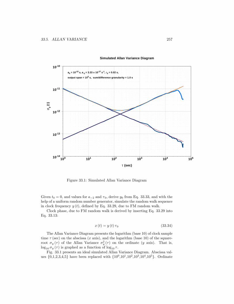
33.5. ALLAN VARIANCE 257
100 101 102 103 104 105
τ (sec)
1014
1013
1012
1011
1010
σ y (τ)
Simulated Allan Variance Diagram
a0 = 1022 s, a2 = 3.33 x 1027 s1, τ0 = 0.02 s,
output span = 105 s, sum/difference granularity = 1.0 s
Figure 33.1: Simulated Allan Variance Diagram
Given t0 = 0, and values for a�2 and �0, derive y0 from Eq. 33.33, and with thehelp of a uniform random number generator, simulate the random walk sequencein clock frequency y (t), de�ned by Eq. 33.29, due to FM random walk.Clock phase, due to FM random walk is derived by inserting Eq. 33.29 into
Eq. 33.13:
x (t) = y (t) �0 (33.34)
The Allan Variance Diagram presents the logarithm (base 10) of clock sampletime � (sec) on the abscissa (x axis), and the logarithm (base 10) of the square-root �y (�) of the Allan Variance �2y (�) on the ordinate (y axis). That is,log10 �y (�) is graphed as a function of log10 � .Fig. 33.1 presents an ideal simulated Allan Variance Diagram. Abscissa val-
ues {0,1,2,3,4,5} have been replaced with {100,101,102,103,104,105}. Ordinate
258 CHAPTER 33. CLOCK MODELING
values {�10,�11,�12,�13,�14} have been replaced with {10�10,10�11,10�12,10�13,10�14}. The Allan root-variance graph approximation from Fig. 33.1 isde�ned by the sum of the two straight lines. Frequency white noise (for a0) isassociated with the straight line with negative slope (�1=2). Frequency randomwalk (for a�2) is associated with the straight line with positive slope (1=2). Thewiggly overlaid functions are reconstructions from simulated data �they becomepoorer approximations as � increases because the sample ensemble is exhausted(becomes smaller) as � increases.
33.5.3 Filter Time Update for Clock
Let tk and tk+1 > tk de�ne the time update interval [tk; tk+1]. Let us denotethe clock �lter transition function �k+1;k, and the clock �lter process noisecovariance Qk+1;k.
State Estimate
State estimate propagation for the clock:
Xk+1jk = �k+1;kXkjk (33.35)
where:
�k+1;k =
�1 (tk+1 � tk)0 1
�(33.36)
Error Covariance
Error covariance propagation for the clock:
Pk+1jk = �k+1;kPkjk�Tk+1;k +Qk+1;k (33.37)
where:
Qk+1;k =
24 ha0 (tk+1 � tk) + a�2 (tk+1 � tk)3i h�a0 + 3a�2 (tk+1 � tk)2
�=2ih�
a0 + 3a�2 (tk+1 � tk)2�=2i
[(a0= (tk+1 � tk)) + 3a�2 (tk+1 � tk)]
35(33.38)
Pjjk =
"P xjjk P xyjjkP yxjjk P yjjk
#, j 2 fk; k + 1g (33.39)
33.5.4 State Estimate Parameters
The fractional frequency y (t) and its generalized integral x (t) is estimated forthe clock.

33.6. ZUCCA-TAVELLA CLOCK MODEL 259
33.6 Zucca-Tavella Clock Model
Following ZT [104] Eq. (19), de�ne
�Y =1
�
Z tk+1
tk
y (t) dt (33.40)
Let E f�g denote the expectation operator, and let �2y (�) denote the Allan Vari-ance, de�ned by (ZT [104] Eq. (18))
�2y (�) =1
2En��Yk+1 � �Yk
�2o(33.41)
Let X1 (t) denote clock phase deviation, let X2 (t) denote the random walkcomponent of clock frequency deviation, and in part, let X3 (t) denote clockfrequency drift (aging). Then
X (t) =
24 X1 (t)X2 (t)X3 (t)
35 (33.42)
Denote initial conditions with
X (0) =
24 X1 (0)X2 (0)X3 (0)
35 =24 c1c2c3
35 (33.43)
Let �1 denote the constant initial frequency o¤set, let a denote deterministicconstant frequency drift, let �2 = a � c3 denote the constant deterministicfrequency aging, and let �3 denote the linear coe¢ cient of the time variationof the frequency drift a. The ZT three-state clock model is de�ned by thestochastic di¤erential equation (ZT [104] Eq. (1))24 dX1 (t)
dX2 (t)dX3 (t)
35 =24 [X2 (t) + �1] dt+ �1dW1 (t)[X3 (t) + �2] dt+ �2dW2 (t)
�3dt+ �3dW3 (t)
35 (33.44)
where t � 0 andW1 (t),W2 (t), andW3 (t) are three independent one-dimensionalstandard Wiener processes. The closed form solution is given by ZT ([104] Equa-tion 5, page 290)
X (t) = � (t; t0)X (t0) +G (t) (33.45)
where
� (t; t0) =
24 1 t� t0 (t� t0)2 =20 1 t� t00 0 1
35 (33.46)

260 CHAPTER 33. CLOCK MODELING
G (t) =
264 �1W1 (t) + �2R t0(t� s) dW2 (t) + �3
R t0
�(t� s)2 =2
�dW3 (s)
�2W2 (t) + �3R t0(t� s) dW3 (s)
�3W3 (t)
375(33.47)
B (t) =
24 t t2=2 t3=60 t t2=20 0 t
35 (33.48)
The error covariance matrix associated with X (t) was presented in Equation33.6 (given initially by ZT ([104] Equation (9) page 290))
Qk+1;k =
264 �21� + �22�3
3 + �23�5
20 �22�2
2 + �23�4
8 �23�3
6
�22�2
2 + �23�4
8 �22� + �23�3
3 �23�2
2
�23�3
6 �23�2
2 �23�
375 (33.49)
ZT derived the Allan Variance �2y (tk; �) of Equation 33.50 (or ZT [104] Equation35) from the Equations above to �nd that the Allan Variance is a function oftk as well as �
�2y (tk; �) =
��21�+�22�
3+�23�
3
20
�+ �23
��3
3+�2tk2
�+�2
2[c3 + �3 [� + tk]]
2
(33.50)The estimation of X3 (t) absorbs �3 and c3. In this sense �3 and c3 are ignorablefor �lter-smoother estimation, and Equation 33.50 becomes
�2y (tk; �) =�21�+�22�
3+23�23�
3
60+�23�
2tk2
(33.51)
But �2y (tk; �), according to Equation 33.51, goes in�nite with increasing tk > 0.ZT have demonstrated that �2y (tk; �) is a useless measure of clock Ci fractionalfrequency stability when �3 > 0. In this case one can use the Hadamard vari-ance, de�ned in ZT Equation (44) and demonstrated to be free of tk in ZTEquation (45), for assessment of clock Ci fractional frequency stability.The ODTK �lter-smoother estimates the 3� 1 matrix clock state X (t) for
each clock Ci according to Equations 33.42 through 33.49, where Qk+1;k is usedfor clock Ci �lter process noise covariance, and the estimation of X3 (t) (aging)is user optional. Allan parameter values for a0, a�2, and ZT di¤usion coe¢ cient�3 are input to the �lter by the user. Allan parameter values for a0 and a�2 canbe determined by the user by inspection of user Allan variance diagram for eachclock Ci. The mapping between ZT di¤usion coe¢ cients, Allan parameters, andGEONS parameters is presented in Table 33.1. The GEONS[31] deterministicrelativistic clock phase drift �dnRRe l
for each satellite clock is modeled in ODTKwith user option selection.

Part VIII
Least Squares (LS)
261


Chapter 34
LS Inputs
34.1 Input Values
Let yj denote a K � 1 column matrix of new measurement values yij , withK measurement types i 2 f1; 2; : : : ;Kg, at measurement time tj , where j 2f1; 2; : : : ;Mg. Thus:
yj =
26664y1jy2j...yKj
37775 (34.1)
Let y denote a KM � 1 column matrix with matrix elements yj :
y =
26664y1y2...yM
37775 (34.2)
Let Wj denote a K � K diagonal matrix of measurement weights at time tj ,where again, superscripts denote measurement types:
Wj =
26664W 1j 0
W 2j
. . .0 WK
j
37775 (34.3)
where:
W ij =
1��ij�2 (34.4)
263
264 CHAPTER 34. LS INPUTS
and where �ij is the error sigma on measurement type i at time tj . Let Wdenote a KM �KM diagonal matrix with diagonal matrix elements Wj :
W =
26664W1 0
W2
. . .0 WM
37775 (34.5)
Let X0jm denote the a priori n�1 matrix state estimate at epoch time t0, wherem denotes the time tm of last measurement used, and the state estimate sizeis n � 6. If t0 = tm, then X0jm = Xmjm = X0j0. Since one can always makethis happen with a state estimate propagation there is no loss of generality inassuming it is true. The state estimate X0j0 always contains a 6�1 matrix orbitestimate Z0j0.
We are given numerical values for the initial state estimate matrix X0j0,measurement matrix y, and measurement weight matrices W . Note: It is oper-ationally conventional to specify Wj as a constant for all tj .
34.2 Initial Calculated Values
34.2.1 Measurement Residuals
Let yi�Xjj0
�denote the nonlinear scalar measurement representation for mea-
surement type i at measurement time tj . Let y�Xjj0
�denote a K � 1 column
matrix of measurement representations yi�Xjj0
�at time tj :
y�Xjj0
�=
26666664y1�Xjj0
�y2�Xjj0
�...
yK�Xjj0
�
37777775 (34.6)
Let �y�Xjj0
�denote the K � 1 column matrix of measurement residuals for
time tj de�ned by:
�y�Xjj0
�= yj � y
�Xjj0
�(34.7)
and adopt the notation:
�yj = �y�Xjj0
�(34.8)
Let �y denote the KM � 1 matrix with matrix elements �yj :

34.2. INITIAL CALCULATED VALUES 265
�y =
26664�y1�y2...
�yM
37775 (34.9)
34.2.2 Partial Derivatives
Let Hij denote the 1 � n measurement-state Jacobian of partial derivatives for
time tj and measurement type i:
Hij =
@yij@Xj
(34.10)
Let �j;0 denote the n�n state-transition matrix Jacobian of partial derivativesfor times t0 and tj :
�j;0 =@Xj
@X0(34.11)
De�ne the 1� n matrix Aij :
Aij = Hij�j;0 (34.12)
Form the K � n matrix Aj :
Aj =
26664A1jA2j...AKj
37775 (34.13)
Form the KM � n matrix A:
A =
26664A1A2...
AM
37775 (34.14)

266 CHAPTER 34. LS INPUTS

Chapter 35
Least Squares Solutions
35.1 LS Normal Equation and Solution
Let X0 denote the true unknown state, let y (X0) denote the unknown measure-ment representation of y as a function of X0, and de�ne a performance functionJ :
J = (y � y (X0))TW (y � y (X0)) : (35.1)
Expand y (X0) about the known state estimate X0j0 in a multi-dimensionalTaylor�s series:
y (X0) = y�X0j0
�+
�@y (X)
@X
�X0j0
�X0 � X0j0
�+ fhigher order termsg (35.2)
De�ne:
A =
�@y (X)
@X
�X0j0
(35.3)
�X0 =hX0 � X0j0
i(35.4)
35.1.1 Linearization
Insert Eq. 35.2 into Eq. 35.1, ignoring higher order terms, to get:
J =�hy � y
�X0j0
�i�A�X0
�TW�hy � y
�X0j0
�i�A�X0
�(35.5)
De�ne:
�y =hy � y
�X0j0
�i(35.6)
267

268 CHAPTER 35. LEAST SQUARES SOLUTIONS
to write:
J (�X0) = (�y �A�X0)TW (�y �A�X0) : (35.7)
Di¤erentiate J with respect to �X0:
@J
@�X0= 2
�ATWA �X0 �ATW�y
�(35.8)
and set the gradient @J=@�X0 equal to zero to �nd extrema. This yields:
ATWA �X0jM = ATW�y; (35.9)
where the use of �X0jM denotes the value of �X0 that extremalizes J (�X0).See Appendix A for details on calculation of the derivative @ ~J=@�X0. Eq. 35.9is called the least squares normal equation. If ATWA is non-singular, the leastsquares solution is obtained by solving Eq. 35.9 for �X0jM , and adding �X0jMto X0j0. Thus:
�X0jM =�ATWA
��1 �ATW�y
�(35.10)
X0jM = X0j0 +�X0jM (35.11)
35.2 Remove the Squaring Operation
Let W 1=2 denote the square root matrix to the diagonal matrix W . That is:W = W 1=2W 1=2. De�ne B = W 1=2A, and b = W 1=2�y. Then Eq. 35.9 can bewritten:
�BTB
��X0jM = BT b (35.12)
Consider the equation:
B �X0jM = b (35.13)
Notice that Eq. 35.12 is rigorously derived from Eq. 35.13 by multiplicationwith BT . These equations are theoretically equivalent. But given a �xed lengthcomputer mantissa, they are not numerically equivalent. This is because the
squaring operation BTB halves the signi�cance of �X0jM
�=�BTB
��1BT b
�relative to the �xed length computer mantissa. A solution of Eq. 35.13 directlyfor �X0jM can recover the lost numerical signi�cance.

35.3. SOLUTION BY TRIANGULARIZATION OF B 269
35.3 Solution by Triangularization of B
The least squares equation:
B �X0jM = b (35.14)
must be solved for �X0jM , where B is a KM�n matrix with rank n, KM � n,and b is an KM � 1 matrix. The solution seems trivial when KM = n:
�X0jM = B�1b (35.15)
ForKM > n, the solution of Eq. 35.14 with greatest numerical stability requiresthe use of orthogonal Householder transformations (Lawson & Hanson [65], page121) for triangularization of matrix B. Our problem is to calculate an acceptablesolution of Eq. 35.14 when KM > n.
35.3.1 Solution Overview
A KM � KM orthogonal matrix T is calculated such that the upper n � nmatrix of the KM � n matrix TB is upper triangular. Then:
TB �X0jM = Tb (35.16)
is easily solved for �X0jM with back substitutions because TB is upper trian-gular.

270 CHAPTER 35. LEAST SQUARES SOLUTIONS

Chapter 36
Least Squares Inadequacies
36.1 LS Measurement Residuals
A fundamental hypothesis for the least squares algorithm says that measure-ment residuals are white noise. This is desireable because white noise residualsdemonstrate the extraction of all information from the measurements. Butanyone performing orbit determination who has examined least squares mea-surement residuals due to processing real data knows that they are seriallycorrelated, not white. This glaring contradiction demonstrates the inadequacyof the least squares algorithm for performing orbit determination.
36.2 Incomplete LS Model
The LS model equation has no structure to account for serially correlated ran-dom gravity modeling errors, serially correlated random air-drag modeling er-rors, and serially correlated random solar pressure modeling errors. These er-rors are absent in the LS state error transition function. The least squaresstate estimate structure is necessarily incomplete because least squares cannotaccomodate random state errors (Bucy and Joseph [9], page 140); e.g., the LSestimated drag coe¢ cient and range bias parameters are necessarily modeled astime constants.
36.3 Least Squares State Error Covariance
The LS state error covariance matrix�ATWA
��1is a function only of the
measurement error covariance matrix W�1. There is no structure here for forcemodeling errors.
271

272 CHAPTER 36. LEAST SQUARES INADEQUACIES
Fit Span T
Position Error
Fit Span T
Position Error
Figure 36.1: Position Error vs Least Squares Fit Span
36.4 Batch Simultaneity
Physically, the alternating e¤ects of force modeling errors on the state estimateand the collection of measurement information for the state estimate evolvessequentially with time. But the least squares algorithm maps measurementinformation at distinct times simultaneously to the state estimate. This providesno time-sequential structure to accomodate force modeling errors.
36.5 Schmidt�s Analysis of Least Squares
Figure 36.1 illustrates Stan Schmidt�s[99] analysis of the ephemeris predictedposition error magnitude in one position component (e.g., intrack), at an arbi-trarily selected �xed prediction time, due to variations in the least squares �tspan T (units time). The green colored function (always decreasing with LS �tspan) is due to measurement error, the red colored function (always increasingwith LS �t span) is due to force model error, and the heavy black function(superposition) is due to the sum of measurement error and force model error.
36.5.1 A Practical Experiment
Figure 36.1 has practical utility. A sample superposition function can be con-structed using real data. Let tBD and tED denote the times of beginning and

36.6. GIBB�S EFFECT 273
end of the tracking data span, let tED be the �xed least squares epoch, and lettP denote a �xed prediction time, where tBD < tED < tP . With tED �xed thepropagation time tP � tED is also �xed. The �t span T = tED� tBD is variable,and thus tBD is variable.First perform a least squares �t with conjectured �t span TC centered on
�xed time tP , and save the resulting ephemeris across time tP . Call this thereference ephemeris. Then perform a sequence j 2 f1; 2; 3; : : :g of least squares�ts where each �t span Tj is distinct, but terminates at the �xed time tED.For each �t propagate an ephemeris across tP , and di¤erence the propagatedephemeris with the reference ephemeris at time tP . Graph the magnitude ofthis di¤erence as a function of Tj to form the superposition from measurementerrors and force modeling errors. If variations in Tj are su¢ ciently small andsu¢ ciently large, the implied superposition function will have negative slope tothe left and positive slope to the right with a unique minimum. Let TBESTdenote the �t span associated with the superposition minimum. Now replaceTC with TBEST and repeat the experiment. Operationally, one must identifythe superposition minimum in order to �optimize� least squares performancefor operational use. The �nal reference ephemeris will have errors, but theirmagnitudes will be small, relative to the errors in the ephemerides used todetermine the "optimal" �t span, if tP � tED is su¢ ciently long.All three functions (red, green, and black) can be graphed quantitatively
using realistic simulated tracking data.
An Unwanted Surprise
Least squares orbit determination has the surprizing property that when oneadds more information (after the resultant superposition minimum) the LS ac-curacy performance gets worse! Generally, LS accuracy performance dependson both data span and data density with time. Performance will also su¤er dueto non-uniform data density with time! Recall Eqs. 35.7, 35.8, and 35.9: Leastsquares chooses a state estimate that minimizes the sum of squares of weightedtracking data residuals. It would be preferable to minimize state estimate errorvariances.
36.6 Gibb�s E¤ect
Our presentation of the Gibbs� e¤ect1 is mentioned here so as to distinguishit from Stan Schmidt�s analysis. Consider �tting any engineering data withuniform density and uniform weight to any appropriate smooth approximatingfunction using a least squares curve �t, where the number of data points isgreater than the number of degrees of freedom in the smooth function.Willard Gibbs noticed that the expected curve �t error magnitudes inside
the data span are always greatest near both ends of the data span. That is,
1An appropriate discussion of the Gibbs E¤ect relating to least squares estimation is pre-sented in a paper by Foster and Richards[24].

274 CHAPTER 36. LEAST SQUARES INADEQUACIES
data neighborhoods containing the points of initiation and termination of dataproduce degraded estimates as compared to data neighborhoods interior to thedata span. The best least squares estimate is at the center of the data span.The least squares signed error envelope can be visualized as a bow tie. TheGibbs�e¤ect contains no notion of force model, and no notion of an arbitrarilyselected �xed prediction point.This is useful for least squares error analysis, but should not be confused
with Stan Schmidt�s analysis. Schmidt refers to a �xed prediction time for leastsquares orbit determination, and compares the e¤ects of measurement error andforce model error due to data span length at that �xed prediction time.

Chapter 37
Tracking Data Editing
One of the most di¢ cult problems in the use of iterated least squares correctionsfor operational orbit determination derives from outliers in the tracking data.Thus tracking data editing is particularly a least squares related problem. Anyleast squares measurement residual variance is useless for tracking data editingbecause the state estimate error variance contribution is always signi�cantlytoo small � due to the absence of a mechanism to represent spacecraft forcemodeling error covariance.
Re�ned least squares tracking data editing is typi�ed by an algorithm toidentify measurement residual magnitudes that are large with respect to theroot mean square (RMS) on the total collection of measurement residuals usedin the least squares batch. This approach is e¤ective when most of the dataare not outliers and when the a priori orbit estimate error magnitudes are suf-�ciently small to enable iterative reduction in the residual RMS. Iterated leastsquares corrections are intended to cope simultaneously with nonlinearities (i.e.,large error magnitudes in the a priori orbit estimate) and with tracking dataediting. When the iterative relative RMS ratio magnitude is reduced to belowan a priori de�ned epsilon, then the iteration is terminated � some say con-verged. But when tracking data are removed from the batch, the residual RMSis rede�ned together with the e¤ective editing policy. Thus the e¤ective editingpolicy is rede�ned on each iteration. It is thus not surprizing that operationalleast squares methods employ a capability to terminate the iterative correctionsarbitrarily after an a priori de�ned maximum iteration count.
Democracy rules: e.g., Given a batch of measurements where seventy percent of the data are biased outliers, the RMS residual editor will throw out thegood data to derive a least squares �t to the outliers.
We shall use the iterative least squares RMS editing method for least squaresorbit determination, but only after the application of every other e¤ective dataeditor. We should note that our autonomous optimal �lter editor should be usedin preference to the iterative least squares RMS editor. Unfortunately, we onlyuse the least squares estimate as a bridge between IOD and �lter initialization.
275

276 CHAPTER 37. TRACKING DATA EDITING
37.1 Tracking Data Editor Identi�cation
Editors are applied to each station pass. Let m denote the number of datasets initially given in the station pass, each at a distinct time, say tk, k 2f1; 2; 3; : : :mg. Each editor will potentially reduce the value of m as outliers arediscarded. In order to complete the station pass editing, a minimum number ofmeasurement sets must survive initial editors.In order to support a successful least squares correction the measurements
must span a particular orbit-period dependent time span. For otherwise, theorbit estimate will be unobservable to the batch of measurements used.The editors identi�ed below are to be applied in the order given.
1. Minimum Number of Data Sets Editor
2. Minimum Time Span Editor
3. Tracking Loop Flag Editor
4. Repeat: Minimum Number of Data Sets Editor
5. Repeat: Minimum Time Span Editor
6. Gross Raw Data Editor
7. Repeat: Minimum Number of Data Sets Editor
8. Repeat: Minimum Time Span Editor
9. Minimum Elevation Editor
10. Repeat: Minimum Number of Data Sets Editor
11. Repeat: Minimum Time Span Editor
12. Sliding Raw Data Polynomial Editor
13. Repeat: Minimum Number of Data Sets Editor
14. Repeat: Minimum Time Span Editor
15. IOD Sliding Fit Kepler Element Editor
16. Repeat: Minimum Time Span Editor
17. Second Di¤erence Editor Using IOD
18. Repeat: Minimum Time Span Editor
19. Residual RMS Editor Criterion Using IOD
20. Repeat: Minimum Time Span Editor
21. Least Squares Solution Attempt

37.2. MINIMUM NUMBER OF DATA SETS EDITOR 277
22. Iterative RMS convergeance
23. Exceed Maximum Iteration Count Editor
24. Manual Editor
25. Select A New Station Pass
26. Measurement Bias Estimate/Guess
27. Call an Orbit Analyst
28. Call AGI
37.2 Minimum Number of Data Sets Editor
Let Tm denote the minimum number of measurement data sets required perstation pass. Let m denote the number of data sets surviving for the stationpass, each at a distinct time, say tk, where k 2 f1; 2; 3; : : :mg.If m < Tm, (default 3) then discard the given station pass, select another,
and begin editing again.
37.3 Minimum Time Span Editor
With some measurement sets the least squares orbit solution is not observablewithout measurements that span a time interval de�ned by multiple orbit pe-riods. Provide a user de�ned constant TMT for minimum time span assoicatedwith each measurement type and assumed orbit class.Let [tB ; tE ] denote the measurement batch time-span currently available. If
jtE � tB j < TMT , acquire more tracking data so as to satisfy the requirement:jtE � tB j � TMT .Note that multiple station passes will probably be required to satisfy this
requirement.
37.4 Tracking Loop Flag Editor
If the measurement �le includes a tracking loop �ag that is set FALSE by sensorhardware, then discard the measurement.
37.5 Gross Raw Data Editor
Let � denote a measurement value of a particular type from a particular mea-surement set. An orbit class, tracking system, and scale factor value S� > 1 areselected by the user for input to the gross editor algorithm. The gross editoralgorithm uses these inputs to de�ne a gross threshold value T� > 0 for each

278 CHAPTER 37. TRACKING DATA EDITING
measurement type �. Let ��f > 0 denote the class dependent, tracking systemdependent, and measurement type dependent upper bound for the error-freecomponent of �. The white noise and bias on � are negligible as compared to��f . Then T� is de�ned by:
T� = S���f
Edit Test: Compare each measurement value magnitude j�j with T�. If j�j < T�,accept measurement � (t). Otherwise discard � (t) and the entire measurementset associated with � (t) at time t.Example: Let � (t) = � (t) denote a range measurement for the SCF tracking
system and a LEO spacecraft. Then � (t) is a two-way range. If the orbitclass is LEO and the spacecraft position vector length rLEO < 1:3er, then��f = 2
p1:32 � 12er = 1:66er. If S� = 1:1, then T� = 1:1 � 1:66er = 1:826er.
Edit test: Given a range measurement � (t), if j� (t)j < 1:826er, accept rangevalue � (t) for processing, otherwise discard � (t) and associated measurementsat time t.Rede�ne m to denote the number of surviving data sets.
37.6 Minimum Elevation Editor
If elevation values Ej are given in the raw data, then reject all surviving mea-surement sets for which Ej < TEL, where
TEL is a user de�ned quantitiy. Default: TEL = 15deg.
37.7 Sliding Raw Data Polynomial Editor
Provide user de�ned constants for polynomial order OP , minimum number ofmeasurements Nm, and RMS epsilon �RMSpoly. Perform a linear least squares �tof an N th order polynomial to an overlapping sliding batch of Nm measurementsfor each measurement type. Calculate a polynomial residual �yj RMS foreach measurement of each �t, then discard each measurement whose residualmagnitude exceeds �RMSpoly. See de�nitions for the polynomial least squaresmethod in the IOD section herein.
37.8 Kepler Element Editor
Perform an IOD sliding �t to all m surviving measurement sets, with each setassociated with a time, say tk, k 2 f1; 2; 3; : : :mg.Example: If IOD is Herrick-Gibbs, then three measurement sets of range,
azimuth, and elevation are required, say at times tj , tj+1, and tj+2, for eachsolution. The �rst Herrick-Gibbs solution for position and velocity componentsat time t2 use measurement sets at times t1, t2, and t3. The second Herrick-Gibbs solution for position and velocity components at time t3 use measurement

37.8. KEPLER ELEMENT EDITOR 279
sets at times t2, t3, and t4. The jth Herrick-Gibbs solution for position andvelocity components at time tj+1 use measurement sets at times tj , tj+1, andtj+2. And the mth Herrick-Gibbs solution for position and velocity componentsat time tm�1 use measurement sets at times tm�2, tm�1, and tm.Transform each solution for position and velocity to Kepler elements.
37.8.1 Kepler Element Bounds Criterion
Check each IOD solution to see that each Kepler element within each solutionis within its formal bound. The following orbit bound de�nitions values shouldbe made consistent with the existing orbit class de�nitions.
LEO 266666641:01er � a < 1:30er
0 � e < 0:10 deg � u < 360 deg0 deg � i � 180 deg0 deg � < 360 deg0 deg � ! < 360 deg
37777775MEO 26666664
1:3er � a < 4:0er0 � e � 0:1
0 deg � u < 360 deg0 deg � i � 180 deg0 deg � < 360 deg0 deg � ! < 360 deg
37777775GPS 26666664
4:0er � a < 4:4er0 � e � 0:1
0 deg � u < 360 deg53 deg � i � 57 deg0 deg � < 360 deg0 deg � ! < 360 deg
37777775SUB-GEO 26666664
4:0er � a < 6:4er0 � e � 0:1
0 deg � u < 360 deg0 deg � i � 180 deg0 deg � < 360 deg0 deg � ! < 360 deg
37777775

280 CHAPTER 37. TRACKING DATA EDITING
GEO 266666646:4er � a � 6:8er0 � e � 0:1
0 deg � u < 360 deg0 deg � i � 180 deg0 deg � < 360 deg0 deg � ! < 360 deg
37777775SUPER-GEO 26666664
6:8er � a � 1000er0 � e � 0:1
0 deg � u < 360 deg0 deg � i � 180 deg0 deg � < 360 deg0 deg � ! < 360 deg
37777775MOLNIYA
266666644:0er � a � 4:4er0:65 � e � 0:75
0 deg � u < 360 deg62 deg � i � 66 deg0 deg � < 360 deg260 deg � ! < 280 deg
37777775HEO 26666664
1:3er � a � 5:0er0:1 � e � 0:999
0 deg � u < 360 deg0 deg � i � 180 deg0 deg � < 360 deg0 deg � ! < 360 deg
37777775OTHER 26666664
?er � a �?er? � e �?
0 deg � u < 360 deg0 deg � i � 180 deg0 deg � < 360 deg0 deg � ! < 360 deg
37777775

37.8. KEPLER ELEMENT EDITOR 281
Measurement Set Selection
Continuing with the Herrick-Gibbs example, Let m � 3 denote a given num-ber of measurement sets within the same tracking station pass, where each setconsists of range, azimuth, and elevation measurements, and each set is asso-ciated with a distinct time tag. Each execution of the Herrick-Gibbs methodrequires the input of three distinct sets of range, azimuth, elevation, and timetag. Transform each solution from position and velocity components to Keplerelements.
37.8.2 m =M = 3
Calculate one Herrick-Gibbs solution for the Kepler element bounds check.
37.8.3 m =M = 4
With m = 4, we can calculate exactly 4 distinct Herrick-Gibbs solutions:�43
�=
4!
3! (4� 3)! = 4
Notice that all four solutions are correlated because at least one of the mea-surement sets used in each solution is also contained in each of the other threesolutions. Name the four measurement sets a; b; c; d, and identify the four solu-tions with: 2664
S1 abcS2 bcdS3 abdS4 acd
3775Each measurement set occurs in exactly three solutions. It is logically impossi-ble that three solutions could succeed and one solution could fail, or that twosolutions could succeed and two solutions could fail. For if two solutions succeed,then measurement sets a; b; c; d are good.Given that all four solutions succeed, then all four measurement sets are
accepted. If exactly three solutions succeed and one solution fails, then rejectall four measurement sets. If exactly two solutions succeed and two fail, thenreject all four measurement sets.Given that one solution succeeds but the other three fail, then three of the
four measurement sets are accepted and one set is discarded. Example: Supposeno bound is violated for solution S1, but violations are incurred for solutionsS2, S3, and S4. Then measurement sets a, b, and c are accepted, and d isdiscarded.
37.8.4 m =M = 5
With m = 5, we can calculate exactly 10 distinct Herrick-Gibbs solutions:

282 CHAPTER 37. TRACKING DATA EDITING
�53
�=
5!
3! (5� 3)! = 10
Name the �ve measurement sets a; b; c; d; e, and identify the ten solutions with:
2666666666666664
S1 abcS2 abdS3 abeS4 acdS5 aceS6 adeS7 bcdS8 bceS9 bdeS10 cde
3777777777777775Each measurement set occurs in exactly six solutions. Given that all ten
solutions succeed, then all ten measurement sets are accepted. Given that foursolutions succeed and six solutions fail, then the one measurement set commonto the six failures is discarded, and the other four measurement sets are ac-cepted. Given that one solution succeeds and nine fail, then accept the threemeasurement sets associated with the successful solution and reject the othertwo measurement sets. For any other combination of success and failures, rejectall �ve measurement sets.
37.8.5 m � 6Process all measurement sets in an overlapping sliding group of �ve, using thelast proceedure for M = 5.Note: We could generalize the combinatorials for any �nite integer m, but
this might be an unusual expense in programming and CPU.
37.8.6 Kepler Element Statistics Criterion
Provide user inputs for constant thresholds Ta, Te, and Ti, with default valuesset to 3. Consider the measurement sets that survive the Kepler Element BoundsCriterion. For each station pass calculate the sample mean �� and sample vari-ance �2� about the mean for Kepler orbit elements � 2 fa; e; ig. Compare eachelement value di¤erence magnitude
��� � ���� with the product of its thresholdwith �� . If
��� � ���� < T��� , then retain the measurement set associated with�, where � 2 fa; e; ig. Otherwise discard the measurement set associated with�. Use the same logic for identi�cation of the measurement set to discard asused for the Kepler Element Bounds Criterion .

37.9. SECOND DIFFERENCE EDITOR USING IOD 283
37.9 Second Di¤erence Editor Using IOD
Calculate measurement residuals (�rst di¤erences) using one orbit estimate fromIOD. See Attachment A for second di¤erence editing.
37.10 Convergence Criteria
37.10.1 Residual RMS Convergence Criterion Using IOD
Provide two user de�ned small positive constants: �RMS (epsilon for root meansquare) and �RRMS (epsilon for relative root mean square).Given measurements yj , j 2 f1; 2; 3; : : : ;mg, calculate measurement residu-
als �yj by propagating one IOD orbit estimate X(0)0 from t0 to tj to get X
(0)j for
each j, by calculating the measurement representation y�X(0)j
�, and by forming
the di¤erences �yj = yj � y�X(0)j
�. De�ne:
Aj =@yj@Xj
@Xj
@X0=
@yj@Xj
�j;0
where theoretically:
�Xj =@Xj
@X0�X0
and de�ne:
�y =
26664�y1�y2...
�ym
37775
A =
26664A1A2...Am
37775Then the root mean square (RMS(k)) on the measurement residuals for iterationk, k 2 f1; 2; : : : ; Lg, is de�ned with:
RMS(k) =1
m
��yT�y
�1=2=
1pm
0@ mXj=1
�y2j
1A1=2
Using least squares, an orbit estimate correction �X(k)0 is derived for iteration
k. Given the orbit estimate correction �X(k)0 , the predicted root mean square
(PRMS) for iteration k = 1 is de�ned by:

284 CHAPTER 37. TRACKING DATA EDITING
PRMS(k) =1pm
���X
(k)0
�TATA
��X
(k)0
�+�yT
��y � 2A�X(k)
0
��1=2If: ��PRMS(k) �RMS(k)
��RMS(k)
< �RRMS
or if:
RMS(k) < �RMS
de�ne convergeance. Otherwise, iterate.
PRMS Derivation
The least squares solution for an iterative linear correction �X0 is derived fromthe approximation:
A�X0�= �y
which has an error �y:
�y = �y �A�X0
De�ne the conditional variance on �y:
�2�y = E
���yj�X0
�T ��yj�X0
��to get:
�2�y =1
m
���X0
�TATA
��X0
�+�yT
��y � 2A�X0
��and assign:
PRMS = ��y
37.10.2 Residual RMS Convergence Criterion After FirstCorrection
If: ��RMS(k+1) �RMS(k)��
RMS(k)< �RRMS
or if:
RMS(k+1) < �RMS
de�ne convergeance. Otherwise, keep iterating.

37.11. RESIDUAL EDITOR 285
37.11 Residual Editor
Compare the magnitude of each measurement residual j�yj j to the product ofa scale factor N (default N = 3) with its unweighted RMS. If:
j�yj j < N RMS, accept the measurement
j�yj j � N RMS, reject the measurement
The RMS is used for editing prior to making each iterative least squares cor-rection.
37.12 Least Squares Solution
Given the application of Editors (1) through (12), attempt a least squares solu-tion with RMS residual editing.
37.12.1 Exceed Maximum Iteration Count Editor
Provide a user de�ned positive constant integer Nmax, to de�ne maximum it-eration count. If the least squares iterations exceed Nmax, then terminate theiterations and invoke the manual editor.
37.13 Manual Editor
Present the user with a graphical display of measurement residuals, and a ca-pability to manually discard each associated measurement.
37.14 Select A New Station Pass
Provide a user de�ned positive constant integer Pmax. Having attempted everyuseful tracking data editing algorithm with subsequent failure in a least squaresattempt on a particular station pass, it is time to discard the entire station pass,select a new station pass, and try again. Discontinue after Pmax station passfailures.
37.15 Measurement Biases
It is possible that all measurements of a particular type are signi�cantly biased;e.g., range transponder bias. If there is a resource available from which to obtaina bias estimate, try that. If not, guess a bias estimate, and try again. Finally,call an orbit analyst for help.

286 CHAPTER 37. TRACKING DATA EDITING

Part IX
Initial Orbit Determination
287


Chapter 38
IOD Methods
Existing validated initial orbit determination (IOD) methods are typically de-pendent on three measurement subsets at three distinct times, where each sub-set contains the same measurement types. From the measurement type set{range, range-rate, azimuth , elevation}, where azimuth and elevation neveroccur separately, there are two subsets of three measurement types: {range,azimuth, elevation}, {range-rate, azimuth, elevation}; there are two subsets oftwo measurement types: {azimuth, elevation}, {range, range-rate}; and thereare two subsets of one measurement type: {range} and {range-rate}. For opera-tional geocentric orbits, validated methods exist for {range, azimuth, elevation},{range-rate, azimuth, elevation}, and {azimuth, elevation}. Two methods areproposed for {range} with six range values. There exist no methods for {range-rate}.Two successfully tested methods are available in ODTK: The Herrick-Gibbs
IOD method[32] for three sets of {range, azimuth, elevation}, and Robert Good-ing�s method[29] for three sets of {azimuth, elevation}.
38.1 Common Modeling Limitations
38.1.1 Two-Body Dynamics
In common, all IOD problems are six-dimensional and nonlinear, and all IODsolutions use two-body gravitational accelerations for orbit propagation. If themeasurement error magnitudes are signi�cant, then the orbit estimate derivedtherefrom with two-body dynamics may be poor.
38.1.2 Measurement Outliers
IOD methods present a measurement editing problem. Gross editing is per-formed on raw tracking data, but exposure to data outliers remains. E¤ectiveand re�ned measurement editing depends on the use of an existing orbit esti-mate, and that does not exist. Thus measurement residuals cannot be formed,
289

290 CHAPTER 38. IOD METHODS
and measurement residual editing is not possible. The success of IOD can bejudged by the success of a subsequent least squares attempt for di¤erential cor-rection to the IOD estimate. Fortunately, with multiple data time points andmultiple IOD data sets, the user is able to attempt an IOD solution many timeswith independent data sets. IOD editing requires manual interaction betweenprogram response and the user.
38.2 Common Equations for IOD
38.2.1 Equation of Motion
The two-body vector equation of motion is given by:
�r = � �
r3r (38.1)
38.2.2 Triangle Geometry
Let us denote the Earth-centered tracking station vector with s. De�ne theinstantaneous range vector � with the vector triangle:
� = r� s (38.2)
de�ne its length � with:
� =p� � � (38.3)
and de�ne the instantaneous unit range vector L with:
L = �=� (38.4)
Then:
r =�L+ s (38.5)
and:
r � r =r2 = �2 + 2�L � s+ s2 (38.6)

Chapter 39
Herrick-Gibbs
Given three distinct sets of range, azimuth and elevation measurements, space-craft position and velocity vectors are calculated according to the method ofGibbs as extended by Herrick [32].
39.1 Position Vectors
Unit range vectors Li with their times ti, for i f1; 2; 3g, are derived directly fromthe three sets of azimuth and elevation measurements, as in the section hereinon station kinematics. Use Eq. 38.5 to form three spacecraft position vectors rifrom measured range measurements �i, station position vectors si, and the Li.
39.1.1 Taylor�s Series
Treat time t2 as �xed so that r2, _r2,. . . are vector time constants. Expand r1and r3 in Taylor�s series about r2:
rj = r2+_r2 (tj � t2)+1
2�r2 (tj � t2)2+
1
3!
...r 2 (tj � t2)3+
1
4!
....r 2 (tj � t2)4+O
�(tj � t2)5
�(39.1)
where j 2 f1; 3g. Ignore O�(tj � t2)5
�to write:
rj = r2+ _r2 (tj � t2)+1
2�r2 (tj � t2)2+
1
3!
...r 2 (tj � t2)3+
1
4!
....r 2 (tj � t2)4 (39.2)
where j 2 f1; 3g. Di¤erentiate Eq. 39.2 twice with respect to tj :
�rj = �r2 +...r 2 (tj � t2) +
1
2
....r 2 (tj � t2)2 (39.3)
Insert Eq. 38.1 twice into Eq. 39.3:
291

292 CHAPTER 39. HERRICK-GIBBS
� �rjr3j= ��r2
r32+...r 2 (tj � t2) +
1
2
....r 2 (tj � t2)2 (39.4)
where j 2 f1; 3g. Solve these two vector equations for ...r 2 and....r 2:
� ...r 2....r 2
�=�
�
�(t3 � t2)2 =2 � (t1 � t2)2 =2� (t3 � t2) (t1 � t2)
� �r2=r
32 � r1=r31
r2=r32 � r3=r33
�(39.5)
where:
� = (t1 � t2) (t3 � t2) (t3 � t1) =2 (39.6)
Insert Eq. 39.5 into Eq. 39.2 to solve for _r2 and �r2 in terms of ri for i 2 f1; 2; 3g.Evaluate the two equations of 39.2 (in terms of _r2, �r2,
...r 2, and
....r 2) as functions
of ri for i 2 f1; 2; 3g. Add these two equations appropriately to get:
r2 = c1r1 + c3r3 (39.7)
_r2 = �d1r1 + d2r2 + d3r3 (39.8)
where:
cj = Aj�1 +Bj=r
3j
�=�1�B2=r32
�, j 2 f1; 3g (39.9)
A1 =t23t13, A3 =
t12t13
(39.10)
B1 = ��t212 + t12t23 � t223
�=12 (39.11)
B2 = ��t212 + 3t12t23 + t
223
�=12 (39.12)
B3 = ���t212 + t12t23 + t223
�=12 (39.13)
t12 = t2 � t1, t13 = t3 � t1, t23 = t3 � t2 (39.14)
and where:
di = Gi +Hi=r3i , i 2 f1; 2; 3g (39.15)
G1 =t223
t12t23t13, G3 =
t212t12t23t13
, G2 = G1 �G3 (39.16)
H1 = �t23=12, H3 = �t12=12, H2 = H1 �H3 (39.17)

39.1. POSITION VECTORS 293
Note: we use r2 as initially derived from Eq. 38.5, rather than from Eq. 39.7.This proves to be successful for radar range measurements and geocentric orbits.Herrick argues that r1; r2; r3 must be forced to be coplanar according to Eq.39.7. Of course r1; r2; r3 are not coplanar due to non two-body perturbativeforces.

294 CHAPTER 39. HERRICK-GIBBS

Chapter 40
Gooding
40.1 Description
40.1.1 Guess Range Values
Given tracking platform positions, GoodingIOD calculates orbit solutions thatcomplete the �rst and third unit range vectors for which pairs of angles areknown but ranges are missing. From each such solution the inertial componentsof position and velocity are automatically implied.Components of unambiguous unit range vector estimates L1, L2 and L3 are
calculated directly from measured angles pairs at times t1, t2, and t3. Unitvectors Lj , j 2 f1; 2; 3g, are accurate three-dimensional direction pointers fromtracking platform to spacecraft, but values for the lengths (ranges) �j of the
range vectors �j = �jLj are unknown. Initial guesses �(0)1 and �(0)3 are de�ned
by the user, or by program default. Vectors L1 and L3 are then multipliedby initial range value guesses �(0)1 and �(0)3 respectively to derive range vectorestimates �(0)1 and �(0)3 at times t1 and t3. Vectors �
(0)1 and �(0)3 are correctly
directed, but their length estimates may be poor. Vectors �(0)1 and �(0)3 areadded to known and accurate platform position vectors s1 and s3 respectivelyat times t1 and t3 to provide spacecraft position vector estimates r
(0)1 = s1+�
(0)1
and r(0)3 = s3 + �(0)3 at times t1 and t3. Errors in the spacecraft position vector
estimates r(0)1 and r(0)3 may be large, in both direction and size. Even so, wehave two spacecraft position vector estimates r(0)1 and r(0)3 at two distinct timest1 and t3.
40.1.2 Lambert
The unknown central angle � between true position vectors r1 and r3, in theplane of r1 and r3, is related to the orbit period P , and measurement time-tagdi¤erence (t3 � t1). For each value of �, and for integers k 2 f0; 1; 2; 3; : : :g,de�ne k such that (k)� < � � (k + 1)�.
295

296 CHAPTER 40. GOODING
Examples: When 0 < � � �, then k = 0, and the central angle � is completelycontained within the �rst one-half orbit. When � < � � 2�, then k = 1, and thecentral angle � is completely contained within one orbit. Thus k is the numberof half-orbits for which the central angle �, between position vectors r1 and r3, iscompletely contained. When the orbit is circular, the relation between (t3 � t1),orbit period P , and k is simple, and the user can make a good guess for k (seeTable 40.2). But when the orbit is highly eccentric, this relation is not obvious.
Lambert Problem
Given values for components of any two distinct spacecraft position vectors r1and r3, and their times t1 and t3, calculate the spacecraft velocity _r1 at timet1, or calculate the spacecraft velocity _r3 at time t3.
Multiple Solutions
When k = 0 or k = 1, Lambert�s Problem has exactly one solution, but whenk � 2, Lambert�s Problem, like a quadratic equation, has two solutions, nosolution, or one solution in a limiting case that occurs with probability zero.Indicator i = 0 if k 2 f0; 1g, but i 2 f0; 1g if k � 2. This Indicates which of twoLambert solutions are to be used, if there are two.
Universal Variables
Gooding�s implementation of the Lambert Problem solution is an accurate, two-iteration universal one, valid for all conic orbits: ellipse, parabola, and hyper-bola.
40.1.3 Gooding
The GoodingIOD algorithm submits r(0)1 and r(0)3 , with times t1 and t3, to theLambert algorithm to calculate velocity _r(0)1 . Although the velocity vector _r(0)1is likely a poor estimate of _r1, at least we have a complete orbit estimate fromr(0)1 and _r(0)1 . This enables the propagation of r(0)1 and _r(0)1 to time t2 to obtainestimates r(0)2 (and _r(0)2 ). Calculate �(0)2 = r
(0)2 � s2, an erroneous estimate of
the true range vector �2. Recall that L2 (from angles data) is a good estimateof the unit range vector at time t2, so project �
(0)2 onto a plane orthogonal to
L2 to de�ne two components of the error in �(0)2 . Now correct �(0)1 and �(0)3 to
reduce the two components of error in �(0)2 , and generate improved estimates�(1)1 and �(1)3 of range, thereby also calculating improved estimates r(1)1 and _r(1)1of position and velocity. This procedure is iterated on integer i so as to drivethe two components of error in �(i)2 to zero, thereby deriving best estimates of�1, �3, r2, and _r2.When the embedded Lambert algorithm provides a solution for the space-
craft velocity _r1 at time t1, then GoodingIOD converges to a local solution for

40.2. A PRIORI ORBIT INFORMATION 297
r2 and _r2. But the price for extraordinary initial errors in �(0)1 and �(0)3 is that
the local solution for r2 and _r2 may not be useful.
Multiple Solutions
When k = 0, there do formally exist either 0, 1, 2, or 3 distinct solutions to theGoodingIOD problem. Unfortunately, there is no sure technique to identify thenumber of distinct solutions a priori. When there are 2 or 3 distinct solutions,only one of them is useful, but we have found that in the large majority of casestested, that one is found. When there are formally 3 distinct solutions, two ofthem may be complex, and will not be found, because the algorithm is restrictedto the real domain.As k is increased, the number of solutions also increases, though only up to
some maximum value. If the value of k is not known in advance, therefore, thesearch for the useful solution can get increasingly complicated.
40.2 A Priori Orbit Information
When there are multiple distinct solutions, only one of them will be useful �associated with the true orbit. It is necessary to correctly couple the selectionsof the three measurement pair time-tags t1, t2, and t3 with the HalfRevEstimate= k from the set f0; 1; 2; 3; : : :g in order to �nd the useful solution. One way todo this is to search through k 2 f0; 1; 2; 3; : : :g beginning with k = 0. But whenthe user has useful a priori information (e.g., orbit class LEO, MEO, GEO,HEO, orbit period P , semi-major axis a, or eccentricity e), then the seach forthe useful solution may be simpli�ed. Table 40.1 correlates orbit class roughlywith P (min), P (sec), a (km), and e.
40.2.1 Near-Circular Orbits
With eccentricity zero (or near zero), any uniform partition of orbit period Pmaps uniformly (or almost uniformly) to increments in central angle � trueargument of latitude di¤erences. This enables association of orbit period Pwith the measurement time-tag di¤erence t3� t1 and the HalfRevEstimate = k.For single-station IOD1 , the simplest approach is to choose k = 0, then selectmeasurements such that 0 < t3 � t1 < P=2, but such that as much of theinterval [t1; t3] is used as possible in this selection so as to attenuate the e¤ectsof measurement white noise. Table 40.2 correlates k with P and t3 � t1.
1Double-station IOD is preferred for accuracy.

298 CHAPTER 40. GOODING
40.2.2 High Eccentricity Orbits
Given an a priori estimate for orbit period P , and knowing that the eccentricitye is large (e.g., e > 0:7), one may choose time-tags t1, t2, and t3 such that0 < t3� t1 < P . Then one must perform two sets of tests with HalfRevEstimate= k, for k = 0, and for k = 1.
40.3 White Noise
Gauss[25] discovered white noise2 on telescopic angles measurements in right as-cension and declination in 1795, while performing orbit determination. All realangles measurements have white noise3 that degrades all algorithms4 for angles-only IOD. For single-station single-pass LEO tracking GoodingIOD overcomesthe white-noise problem when t3 � t1 > 0 is su¢ ciently large. For two-stationLEO tracking, GoodingIOD signi�cantly reduces position and velocity errorsdue to white-noise, relative to single-station tracking, if all measurements areselected from a common six minute time interval and t3 � t1 = 1min approxi-mately.
40.4 Tropospheric E¤ects
Degrading e¤ects of the troposphere, from ground based platforms, can be sig-ni�cantly reduced by selecting measurements whose elevations are greater than10 deg.
40.5 Inspection of Kepler Orbit Element Values
Given a priori information regarding the orbit, and given multiple solutions fromthe same measurement set, the user can frequently eliminate useless solutionsby inspection of the Kepler orbit elements, particularly the semi-major axis andeccentricity.
40.6 Multiple Solutions from Each Set of Dis-tinct Measurement Sets
Comparison of sets of multiple solutions from distinct measurement sets may,or may not, identify the useful solution.
2Gauss[25] invoked the normal density function to model white noise, and invented theiterative least squares algorithm (1795) to perform orbit determination on an overdeterminedset of telescopic measurements in right ascension and declination.
3Practically, a realizable white noise time sequence may be visualized as a random normalsequence where every component is independent of all others (no serial correlation), and wherethe ensemble variance is �nite.
4The classical LaPlace IOD method is destroyed by white noise if its RMS is signi�cant,when applied to geocentric orbits .

40.7. LEAST SQUARES 299
40.7 Least Squares
Given multiple solutions from the same measurement set, the user can test eachsolution by running least squares on it with an overdetermined set (more thanthree) of angles measurements. Least squares will converge only on the usefulsolution.

300 CHAPTER 40. GOODING
Orbit Class P (min) P (sec) a (km) eLEO 100 6000 7137 0:000 < e < 0:050GEO 1436 86169 42163 0:000 < e < 0:001GPS (MEO) 718 43080 26560 0:000 < e < 0:001HEO 718 43080 26561 0:7 (Molniya)
Table 40.1: Mean Orbit Period vs Orbit Class
t3 � t1 vs P k0 < t3 � t1 < P=2 0P=2 < t3 � t1 < P 1P < t3 � t1 < (3=2)P 2(3=2)P < t3 � t1 < 2P 3...
...
Table 40.2: Orbit Period Relations

Part X
Tracking and Data RelaySatellite System (TDRSS)
301


Chapter 41
TDRSS Range and Doppler
Simultaneous orbit determination of multiple TDRS (GEO) orbits and multi-ple LEOs and/or MEOs is enabled with the implementation of capabilities toprocess four-legged range and �ve legged Doppler measurements for NASA�sTelemetry and Data Relay Satellite System (TDRSS). NASA�s associated Bi-lateral Ranging Transponder System (BRTS) range and Doppler measurementscan also be processed to perform orbit determination on each TDRS separately,or on all TDRS� simultaneously by fusing BRTS measurements with TDRSSmeasurements. Radio signals for measurements in the same round-trip linkare all generated by the same atomic ground clock, and are said to be coher-ent because the e¤ects of clock phenomenology and relativity are subtractedout. That is, the four-legged range and �ve legged Doppler measurements aretwo-way measurements.Both of the two time-varying transponder biases in the four legged range link
may be estimated, separately1 or simultaneously, with ground station rangebiases. Also, time-varying range-sum biases can be estimated to include thesummed e¤ects of transponder biases and ground station biases.
41.1 TDRSS Range Vectors
TDRS refers to a Tracking and Data Relay Satellite. The Tracking and DataRelay Satellite System (TDRSS) consists of a constellation of geosynchronousTDRS, a constellation of LEO spacecraft, the White Sands Ground Terminal(WSGT), associated hardware and software, and personnel. Fig. 41.1 depictsthe Earth centered positions of the WSGT at times t0 and t4 with positionvectors S0 and S4. Consider a radio plane wave that is emitted from the WSGTat time t0, received and retransmitted by a TDRS transponder at time t1,received and retransmitted by a LEO spacecraft transponder at time t2, receivedand retransmitted by the TDRS transponder at time t3, and received by the
1Time-constant values for the two transponder biases in the four legged range link wereshown to be simultaneously observable when ground station range biases are known a priori.
303

304 CHAPTER 41. TDRSS RANGE AND DOPPLER
t0 t4
t2
t1t3
C
ρ34
ρ12
ρ23
ρ01
S0S4
Figure 41.1: Four TDRSS Range Vectors
WSGT at time t4. Fig. 41.1 identi�es associated range vectors �01, �12, �23,and �34. Let us denote TDRS position vectors by Rj at tj , and LEO spacecraftposition vectors by rj at tj , for j 2 f1; 2; 3g. De�ne spacecraft position vectors:
R1 = S0 + �01 (41.1)
r2 = R1 + �12 (41.2)
R3 = r2 + �23 (41.3)
and the WSGT vector constraint:
S4 = R3 + �34 (41.4)
41.2 Range Sum
The following construction assumes that all range e¤ects associated with cabledelay, electromagnetic phase center, Faraday rotation, relative rotation betweenantennas, transponders, troposphere, and ionosphere are addressed elsewhere.
41.2. RANGE SUM 305
41.2.1 Range Elements
De�ne:
t(j)(j+1) = tj+1 � tj , tj < tj+1, j 2 f0; 1; 2; 3g (41.5)
De�ne range elements:
�01 =p�01 � �01 = ct01 (41.6)
�12 =p�12 � �12 = ct12 (41.7)
�23 =p�23 � �23 = ct23 (41.8)
�34 =p�34 � �34 = ct34 (41.9)
Each range element is de�ned by two expressions, a geometric expression and aradio wave propagation time delay expression.
41.2.2 Range Sum De�nition
Let us denote the two-way range sum with �0L, and de�ne it with:
�0L = �01 + �12 + �23 + �34 = ct0L (41.10)
where:
L = 4 (41.11)
41.2.3 Range Sum Time Tag
The range sum time tag is de�ned by tL = t4.
41.2.4 Construction of the Range Sum Representation
Range Iterations
Given the time-tag tL = t4, we wish to calculate a �rst approximation ~�34 for�34. Evaluate S4 at tL = t4. Let us denote a �rst approximation for timedi¤erence t34 with ~t34 and set ~t34 = 0:133s. Then from Eq. 41.5:
~t3 = t4 � ~t34Evaluate ~R3 at ~t3. Rearrange Eq. 41.4 to approximate the range vector �34:
~�34 = S4 � ~R3
Use Eq. 41.9 to calculate the range approximation:

306 CHAPTER 41. TDRSS RANGE AND DOPPLER
~�34 =p~�34 � ~�34
and use Eq. 41.9 again to calculate a second approximation for t3;4:
�t3;4 = ~�34=c
Set ~t3;4 = �t3;4 and iterate on the above sequence until:��~t3;4 � �t3;4�� < �3;4
to yield t3, t34, and �34. Three iterations are usually su¢ cient.Given the time t3, calculate t2, t23, and �23 as above. Given the time t2,
calculate t1, t12, and �12 as above. Given the time t1, calculate t0, t01, and �01as above.
Range Sum
Now use Eq. 41.10 to calculate the range sum �0L.
41.3 Range Sum Partial Derivatives
41.3.1 Eliminate Light-Time
Simple and su¢ cient measurement to state partial derivative approximationsare achieved by eliminating light-time e¤ects:
�1 � �01 = ��34 (41.12)
�2 � �12 = ��23 (41.13)
S � S0 = S4 (41.14)
R � R1 = R3 (41.15)
r � r2 (41.16)
�1 =p�1 � �1 (41.17)
�2 =p�2 � �2 (41.18)
all de�ned at the same epoch t = t4.

41.3. RANGE SUM PARTIAL DERIVATIVES 307
41.3.2 Simpli�ed Expressions
Then:
r = S+ �1 + �2 = R+ �2 (41.19)
R = S+ �1 (41.20)
De�ne the one-way range sum approximation with:
� = �1 + �2 =p�1 � �1 +
p�2 � �2 (41.21)
41.3.3 Di¤erentials
Di¤erentiate Eqs. 41.19 and 41.20:
�r = �S+ ��1 + ��2 = �R+ ��2 (41.22)
�R = �S+ ��1 (41.23)
Di¤erentiate Eq. 41.21:
�� = �1 � ��1 + �2 � ��2 (41.24)
where:
�1 = �1=�1 (41.25)
�2 = �2=�2 (41.26)
41.3.4 LEO Satellite Range Sum Partials
Vary r, but with S and R held �xed. Then:
�S =�R = 0 (41.27)
And from Eq. 41.23:
��1 = 0 (41.28)
According to Eq. 41.22:
�r = ��2 (41.29)
and from Eq. 41.24:
�� = �2 � �r (41.30)
Now �r has the decomposition on the inertial frame:

308 CHAPTER 41. TDRSS RANGE AND DOPPLER
�r =3Xj=1
(�r � ij) ij =3Xj=1
�zjij (41.31)
where:
�zj = �r � ij (41.32)
Note that:
�� =3Xj=1
@�
@zj�zj (41.33)
So insert Eq. 41.31 into Eq. 41.30:
�� =3Xj=1
(�2 � ij) �zj =3Xj=1
@�
@zj�zj (41.34)
from which:
@�
@zj= �2 � ij , j 2 f1; 2; 3g (41.35)
The LEO position partials are just the inertial components of the unit rangevector �2, where from Eq. 41.19:
�2 = r�R (41.36)
�2 = �2=�2 (41.37)
De�ne the 1� 3 matrix @�=@z:
@�
@z=h
@�@z1
@�@z2
@�@z3
i(41.38)
Instantaneously, variations in _r leave r invariant, thus:
@�
@ _z= 01�3 (41.39)
For LEO, de�ne:
Z =
�z_z
�(41.40)
Then the 1 � 6 matrix of range sum with respect to LEO ECI postion andvelocity partials is de�ned by:
@�
@Z=�@�@z
@�@ _z
�(41.41)
41.3. RANGE SUM PARTIAL DERIVATIVES 309
41.3.5 TDRS Range Sum Partials
Vary R, but with S and r held �xed. Then:
�S =�r = 0 (41.42)
and from Eq. 41.23:
��1=�R (41.43)
From Eq. 41.22:
��2=� ��1 (41.44)
So:
��2=� �R (41.45)
Then from Eq. 41.24:
�� = (�1 � �2) � �R (41.46)
Now �R has the decomposition on the inertial frame:
�R =
3Xj=1
(�R � ij) ij =3Xj=1
�z0
jij (41.47)
where:
�z0
j = �R � ij (41.48)
Note that:
�� =
3Xj=1
@�
@z0j
�z0
j (41.49)
So insert Eq. 41.47 into Eq. 41.46:
�� =3Xj=1
[(�1 � �2) � ij ] �z0
j =3Xj=1
@�
@z0j
�z0
j (41.50)
from which:
@�
@z0j
= (�1 � �2) � ij , j 2 f1; 2; 3g (41.51)
The TDRS position partials are just the inertial components of the range vectordi¤erence (�1 � �2). De�ne the 1� 3 matrix @�=@z
0:
@�
@z0=h
@�
@z01
@�
@z02
@�
@z03
i(41.52)

310 CHAPTER 41. TDRSS RANGE AND DOPPLER
Instantaneously, variations in _R leave R invariant, thus:
@�
@ _z0= 01�3 (41.53)
For TDRS, de�ne:
Z0=
�z0
_z0
�(41.54)
Then the 1 � 6 matrix of range sum with respect to TDRS ECI postion andvelocity partials is de�ned by:
@�
@Z 0 =h
@�
@z0@�
@ _z0
i(41.55)
41.4 Doppler Measurements
De�ne symbols:
fT reference transmit frequencyfD instantaneous Doppler frequencyfP pilot tone frequencyc speed of light in vacua_�01 leg 1 instantaneous range-rate_�12 leg 2 instantaneous range-rate_�23 leg 3 instantaneous range-rate_�34 leg 4 instantaneous range-rate_�P instantaneous pilot tone range-rate
Table 41.1: Doppler Measurement Symbol De�nitions
The Doppler frequency fD extracted from the TDRSS receiver hardware hasthe form:
fD = �1
c
24fT 4Xj=1
_�(j�1)(j) + fP _�P
35 (41.56)
Integrate Eq. 41.56 across the carrier phase integration interval [tL; tL+1], thendivide through by (tL+1 � tL), to de�ne the TDRSS Doppler measurement rep-resentation �fD:
�fD � �1
tL+1 � tL
Z tL+1
tL
fDdt

41.5. DOPPLERPARTIALS 311
= � 1
c (tL+1 � tL)
24fT 4Xj=1
Z tL+1
tL
_�(j�1)(j)dt+ fP
Z tL+1
tL
_�P dt
35 (41.57)
Each integral on the right hand side has the form:Z tL+1
tL
_�dt =
Z tL+1
tL
d� = � (tL+1)� � (tL) (41.58)
With these integrations, the TDRSS Doppler measurement representation �fD(Eq. 41.57) becomes:
�fD = �1
c (tL+1 � tL)
24fT 4Xj=1
��(j�1)(j) + fP��P
35 (41.59)
where:
��(j�1)(j) = �(j�1)(j) (tL+1)� �(j�1)(j) (tL) (41.60)
��P = �p (tL+1)� �p (tL) (41.61)
41.5 DopplerPartials
The time tags for Doppler measurements are at tL+1, and the orbit estimate:
Z (tL+1) =
�z (tL+1)_z (tL+1)
�will sit nominally at tL+1. Thus the �rst term in the �rst and second terms ofEqs. 41.63 and 41.64 is already calculated for range sum partials. The secondterm in the �rst and second terms of Eqs. 41.63 and 41.64 will require the useof the linear transition function � (tL; tL+1) to move the calculation of the 1�6matrix @� (tL) =@Z (tL) from time tL to time tL+1:
@� (tL)
@Z (tL+1)=@� (tL)
@Z (tL)
@Z (tL)
@Z (tL+1)=@� (tL)
@Z (tL)� (tL; tL+1) (41.62)
41.5.1 LEO Satellite Doppler Partials
Di¤erentiate Eq. 41.59:
@ �fD@z
= � 1
c (tL+1 � tL)
24fT 4Xj=1
@�(j�1)(j) (tL+1)� �(j�1)(j) (tL)@z (tL+1)
+ fP@�p (tL+1)� �p (tL)
@z (tL+1)
35(41.63)

312 CHAPTER 41. TDRSS RANGE AND DOPPLER
41.5.2 TDRS Doppler Partials
Di¤erentiate Eq. 41.59:
@ �fD@z0
=
� 1
c (tL+1 � tL)
24fT 4Xj=1
@�(j�1)(j) (tL+1)� �(j�1)(j) (tL)@z0 (tL+1)
+ fP@�p (tL+1)� �p (tL)
@z0 (tL+1)
35(41.64)

Chapter 42
One-Way Return-LinkDoppler
The TDRSS one-way return-link three-legged Doppler measurement �lter capa-bility has been implemented according to GSFC documentation.
313

314 CHAPTER 42. ONE-WAY RETURN-LINK DOPPLER

Part XI
Global Positioning System(GPS) Low Earth Orbit
(LEO) Receivers
315


Chapter 43
Pseudo-Range Filtering
43.1 Introduction
The USER spacecraft pseudo-range measurement representation chain (Eq. 43.1)is adopted from JPL[130], but the components in that chain are inappropriate,in part, due to JPL modeling of the USER clock as a ground �xed clock. Also,the JPL document does not derive relativistic expressions from �rst principles.This makes it di¢ cult to validate the JPL equations. We have derived appropri-ate expressions from the Schwarzschild metric that enable the reader to validatethe equations we have provided.Measurement-to-state analytical partial derivative approximations for USER
GPS psuedo-range measurements are derived and given by Eqs. 43.81 through43.86.The USER stochastic clock model is derived from Allan[1]. From this clock
model, the �lter GPS USER clock propagation, transition, covariance propaga-tion, and process noise covariance functions are derived and given in Eqs. 33.35,33.36, 33.37, and 33.38 respectively.The synchronization of USER spacecraft clock to NAVSTAR SV clock is
discussed.
43.1.1 Pseudo-Range Option
�A properly equipped receiver will detect amplitude, pseudo-range and phasemeasurements for each of the C/A, L1 P-code (P1) and L2 P-code (P2) sig-nals. The C/A and P1 measurements essentially contain identical information,however C/A is preferred over P1 because its power is stronger by 3 dB andis not encrypted. Therefore, the basic observables used during an occultationexperiment are the C/A phase and the P2 phase measurements between the low-Earth orbit (LEO) satellite and the occulting GPS satellite� (Kursinski [56]).This conclusion applies as well to orbit determination. Therefore, we shouldprovide an option to remove ionosphere with either {P1,P2} or {C/A,P2}.
317

318 CHAPTER 43. PSEUDO-RANGE FILTERING
43.2 USER GPS Pseudo-Range
43.2.1 Pseudo-Range
Let us denote the pseudo-range measurement representation by �, and de�ne itwith:
� = c��T 3 � �3
�+��3 � t3
�+�t3 � t2
�+�t2 � �2
�+��2 � T 2
��+ �
= c�T 3 � T 2
�+ � (43.1)
where c is speed of light in vaccuo, � is a stored constant (range bias), and timenotations are identi�ed below.
43.2.2 Range Measurement Time Notation
T 3 receiver time tag�3 receiver proper timet3 receiver coordinate time (TDT)t2 transmitter coordinate time (TDT)�2 transmitter proper timeT 2 transmitter time tag
43.2.3 Time Di¤erencesT 3 � �3 receiver clock error (user spacecraft clock)�3 � t3 receiver proper time - receiver coordinate timet3 � t2 receiver coordinate time - transmitter coordinate timet2 � �2 transmitter coordinate time - transmitter proper time�2 � T 2 transmitter clock error (GPS NAVSTAR clock)
43.2.4 Receiver Clock Errors
The receiver clock error T 3 � �3 will be composed of two additive components:a stored constant bias scalar �x and a clock phase state estimate parameterx, de�ned by Eqs. 33.23 and 33.13. The generalized derivative y = dx=dt,de�ned by Eqs. 33.29 and 33.13, will also be estimated, and is associated withan additive constant bias scalar �y. The coupled errors in the two-parameterclock state estimate will be accounted for with a 2x2 state estimate clock errorcovariance. The 2x2 clock transition matrix function is de�ned by Eq. 33.36,and the 2x2 clock process error covariance matrix function is de�ned by Eq.33.37.Any long term estimated constant biases (e.g., clock synchronization error
and drift) in x and y will be transferred manually to the unestimated parameters�x and �y.The state estimate is composed of clock modeling e¤ects, and non-clock
modeling e¤ects �non-separable from clock modeling e¤ects.

43.2. USER GPS PSEUDO-RANGE 319
Clock modeling e¤ects
� Synchonization error between receiver clock and transmitter clock (as-sumed here to be due to the receiver clock)
� Stochastic phenomenology of the receiver clock (assumed here to be infe-rior to the NAVSTAR clock)
� NAVSTAR transmitter clock error due to modeling and propagation errorsin the coe¢ cients downlinked in the navigation message
Non-clock modeling e¤ects due to modeling errors
� NAVSTAR propagation errors in position
� Antenna multipath (spacecraft body speci�c)
� Antenna phase center location
� Mutual rotations of transmitting and receiving antennas
� Troposhere
� Ionosphere
� Faraday rotation
� Unmodeled cable lengths in the hardware
43.2.5 Receiver Proper Time less Receiver Coordinate Time(User Spacecraft)
For this subsection we shall drop the superscript 3 that identi�es the receiverand add a subscript j that distinguishes time. Thus: �3 = � j and t3 = tj , forj 2 fk; k + 1g. From 43.28, de�ne the sequential �lter time-update calculation:
(�k+1 � tk+1) = (�k � tk)� (tk+1 � tk)3�
2ac2� 2
c2�rk+1 _rk+1 � rk _rk
�(43.2)
where k 2 f0; 1; 2; : : :g. The relation between �0 and t0 is arbitrary. For initial-ization1 we choose to de�ne:
�0 = t0 (43.3)
The relativistic constant clock phase bias, in the User spacecraft clock, is con-tained in its proper time �0 at initialization of sequential orbit determination.
1The JPL initialization convention is de�ned by:
�0 � t0 = � [(TAI � UTC) + (TDT � TAI)]

320 CHAPTER 43. PSEUDO-RANGE FILTERING
This is of course relevant only for receivers that do not perform clock steering.For in this case, GPS range measurements from di¤erent receiver channels mustbe di¤erenced at the same instant to remove the e¤ects of clock steering, andthus remove all User clock e¤ects for orbit determination.
43.2.6 Coordinate Time Di¤erence
Coordinate times are in TDT. The coordinate time di¤erence�t3 � t2
�is asso-
ciated with the positional coordinate di¤erences of ECI ICRF ephemerides, andis given:
t3 � t2 = r32c+2�
c3ln
�r3 + r2 + r32r3 + r2 � r32
�(43.4)
This light-time equation is due to Holdridge[36]. The unknown quantitiy t2
(coordinate time of transmission) can be calculated by Newton-Raphson ([130]Eq. 4.2.3.1.19 �note mislabel here):
t2(i+1) = t2(i)+
"t3 � t2(i) �
2�
c3ln
r3 + r
(i)2 + r
(i)32
r3 + r(i)2 � r(i)32
!!#=h1� r(i)32 � _r
(i)2 =
�cr(i)32
�i(43.5)
where for i = 0, and t2(i) = t2(0):
t2(0) = t3
43.2.7 Transmitter Coordinate Time less Transmitter ProperTime (NAVSTAR)
For this subsection we shall drop the superscript 2 that identi�es the transmitterand add a subscript j that distinguishes time. Thus: �2 = � j and t2 = tj , forj 2 fk; k + 1g. The following equations (derived below) are equivalent:
(tk+1 � �k+1) = (tk � �k) + (�k+1 � �k)3�
2ac2+2
c2�rk+1 _rk+1 � rk _rk
�(43.6)
(tk+1 � �k+1) = (tk � �k) + (�k+1 � �k)3�
2ac2+2ep�a
c2(sinEk+1 � sinEk)
(43.7)The constant clock rate 3�=
�2ac2
�is accounted for by o¤setting the frequency
of the onboard NAVSTAR oscillator. So set:
(�k+1 � �k)3�
2ac2= 0 (43.8)

43.2. USER GPS PSEUDO-RANGE 321
43.2.8 Transmitter Clock Error
This section identi�es the term��2 � T 2
�for the range representation de�ned
by Eq. 43.1.Each NAVSTAR Space Vehicle (SV) keeps its own SV Time with its own
SV clock. SV Time is a proper time. According to ICD-GPS-200C, paragraph20.3.3.3.3.1, page 88, the user transforms SV Time to GPS Time2 t using equa-tions given there, together with clock values given in each HANU message. GPSTime t is a coordinate time. Given the evaluation of ICD Eq. (1):
t = tSV ��t (43.9)
and ICD Eq. (2):
�tSV = af0 + af1 (t� t0c) + af2 (t� t0c)2 +�tr (43.10)
then time of radio wave front emission from the NAVSTAR SV in coordinatetime is t (GPS Time). There are two signi�cant facts to note here: (i) SV Timeis a NAVSTAR clock proper time, and (ii) GPS Time is a relativistic coordinatetime. Note that there are no leap seconds in GPS Time. As noted in the ICD,ICD Eqs. (1) and (2) are coupled: Approximate t by tSV in ICD Eq. (2).ICD-GPS-200C, presents three relativistic expressions:
�tr = Fe�A1=2
�sinEk (43.11)
F =�2�1=2c2
(43.12)
�tr = �2~R � ~Vc2
(43.13)
The right-hand side of Eq. 43.11, using Eq. 43.12, is found in the derivationof Eqs. 43.30 and 43.32. The right-hand side of Eq. 43.13, is found in thederivation of Eqs. 43.28 and 43.29. Thus the use of �tr converts SV Time (aproper time) to GPS Time (a coordinate time). Therefore use Eq. 43.29 orEq. 43.31 to explain the conversion of NAVSTAR proper time to NAVSTARcoordinate time. It is clear that the ICD expressions must be applied twice: attk and at tk+1. ICD-GPS-208, Section 20.1, presents a related discussion forthe HANU.The frequency of each NAVSTAR SV clock is physically o¤set to negate
the e¤ect of the rate 3�=�2ac2
�in the term (�k+1 � �k)
�3�=
�2ac2
��in Eqs.
43.29 and 43.31. ICD-GPS-200C, Section 20.3.3.3.3.1, page 11, states that theNAVSTAR transmitted frequency is biased (for general relativity) by �f=f =�4:464 � 10�10 with �f = �4:5674 � 10�3Hz so that the nominal frequencyto a user on the ground is 10:23MHz. Note: Each NAVSTAR orbit hasaNAV STAR = 4:2er. If the bias is designed for the USER at aUSER = 1:0er,
2The ICD uses t for GPS Time. I use t for TDT Time. Distinguish them by context.

322 CHAPTER 43. PSEUDO-RANGE FILTERING
there is an obvious error for a USER orbit with a > 1:0er. But this will perfectlyalias into the phase rate estimate.
43.3 Schwarzschild Metric
Einstein�s gravitational �eld equation (1916):
G�� = 8�T��
with second order tensors G�� and T�� , is a simple and beautiful expressionto physicists, but is di¢ cult to apply to solutions of real problems �by math-ematicians and engineers. Time and space are coupled on a four-dimensionalhypersurface (manifold). After selection of coordinates, this equation generatesa second order nonlinear partial di¤erential equation in four dimensions. Toapply this equation, one must �nd an appropriate metric that is consistent withit. Two exact metric solutions (line elements) have been found, one by KarlSchwarzschild (1916) and one by Roy Kerr (1963), and a host of approximatesolutions, referred to as Post-Newtonian approximations, are in use. Each metricis a scalar nonlinear ordinary �rst order di¤erential equation. The Schwarzschildmetric refers to a static non-rotating mass distributed in spherical concentriclayers3 . The Kerr metric refers to a rotating mass, and models its quadrapole(J2). There exists a small group of relativists who have been seeking other exactsolutions for many years. The Schwarzschild metric is su¢ cient (TBR) for ourmodeling of GPS clocks.The Schwarzschild metric can be found multiple times with a WEB search,
and is given by several authors of books on general relativity; e.g., Moller[83],Moller Eqs 11.83 and 11.88. The Schwarzschild metric can be written in severalforms, one of which is:
ds2 =
�1� 2�
c2r
�c2dt2 �
�1� 2�
c2r
��1dr2 � r2
�d�2 + sin2 �d'2
�(43.14)
where:
c speed of light� gravitational constantds interval in 4d (like distance in 3d)dt coordinate time intervald� proper time intervalr radial distance from Earth CM to clock� codeclination of clock' right ascension of clock
ds = cd� (43.15)
3This is a crude model for our earth.

43.3. SCHWARZSCHILD METRIC 323
and the 3�1 matrix of inertial Earth centered position components for the clockare de�ned: 24 x1
x2x3
35 =24 r sin � cos'r sin � sin'r cos �
35 (43.16)
43.3.1 Proper Time vs Coordinate Time
De�ne clock speed squared with _s2:
_s2 =3Xj=1
_x2j (43.17)
to �nd:
_s2 = _r2 + r2�_�2+ _'2 sin2 �
�(43.18)
Expand�1� 2�=
�c2r���1
, retain terms to O(c�2), and insert into Eq. 43.14:
ds = cdt
�1� 1
c2
�2�
r+ _r2 + r2
�_�2+ _'2 sin2 �
���1=2(43.19)
Insert Eqs. 43.15 and 43.18 into Eq. 43.19:
d� = dt
s1� 1
c2
�2�
r+ _s2
�(43.20)
Expand the radical and truncate to order O�c�4�to get:
d� = dt
�1� 1
c2
��
r+_s2
2
��(43.21)
dt = d�
�1 +
1
c2
��
r+_s2
2
��(43.22)
Potential energy �=r captures general relativity, and kinetic energy _s2=2 cap-tures special relativity, according to the Schwarzschild metric.
43.3.2 Time Integrals
De�nite time integrals of Eqs. 43.21 and 43.22 provide transformations be-tween proper time � and coordinate time t. Our use of tk and tk+1 refers toour ODTK �lter time-update function. For implementation, we require stateestimate values at both tk and tk+1, in coordinate time TDT. Thus:
(�k+1 � �k) = (tk+1 � tk)�1� 3�
2ac2
��2ep�a
c2(sinEk+1 � sinEk) (43.23)

324 CHAPTER 43. PSEUDO-RANGE FILTERING
(tk+1 � tk) = (�k+1 � �k)�1 +
3�
2ac2
�+2ep�a
c2(sinEk+1 � sinEk) (43.24)
where classical expressions from two-body astrodynamics have been used:
r = a (1� e cosE)
M =M0 + n (t� t0) = E � e sinE
_M = n = _E (1� e cosE)
dt =
�a3=2p�
�(1� e cosE) dE
n2a3 = �
Since:
p�ae sinE = r _r = r � _r (43.25)
then equivalently:
(�k+1 � �k) = (tk+1 � tk)�1� 3�
2ac2
�� 2
c2�rk+1 _rk+1 � rk _rk
�(43.26)
(tk+1 � tk) = (�k+1 � �k)�1 +
3�
2ac2
�+2
c2�rk+1 _rk+1 � rk _rk
�(43.27)
Rearrange the last two equations:
(�k+1 � tk+1) = (�k � tk)� (tk+1 � tk)3�
2ac2� 2
c2�rk+1 _rk+1 � rk _rk
�(43.28)
(tk+1 � �k+1) = (tk � �k) + (�k+1 � �k)3�
2ac2+2
c2�rk+1 _rk+1 � rk _rk
�(43.29)
or, using Eq. 43.25 again:
(�k+1 � tk+1) = (�k � tk)� (tk+1 � tk)3�
2ac2�2ep�a
c2(sinEk+1 � sinEk)
(43.30)

43.4. GROUP DELAY DIFFERENTIAL 325
(tk+1 � �k+1) = (tk � �k) + (�k+1 � �k)3�
2ac2+2ep�a
c2(sinEk+1 � sinEk)
(43.31)Add (tk+1 � �k+1), according to Eqs. 43.29 or 43.31, to proper time �k+1 toget coordinate time tk+1. Add (�k+1 � tk+1), according to Eqs. 43.28 or 43.30,to coordinate time tk+1 to get proper time �k+1.Run a minus sign through Eq. 43.28:
(tk+1 � �k+1) = (tk � �k) + (tk+1 � tk)3�
2ac2+2
c2�rk+1 _rk+1 � rk _rk
�(43.32)
and compare Eq. 43.32 to Eq. 43.29. They are di¤erent; i.e., we have implicitlyassumed that (tk+1 � tk) 3�
2ac2 is negligibly di¤erent than (�k+1 � �k)3�2ac2 . This
is due to the above truncation to order O�c�4�(TBR).
43.3.3 JPL Model
Comparison of the equations above to those of JPL[130] enables identi�cationof terms for a USER ground clock in the JPL document, inappropriate for aUSER spacecraft clock in free-fall.
43.4 Group Delay Di¤erential
From paragraph 3.3.1.7.2 of the ICD-GPS-200C[40], there exists a NAVSTARdependent group delay di¤erential between the radiated L1 and L2 signals whosemagnitude can be as large as 15ns; i.e., 15ft. From paragraph 20.3.3.3.1.8:"Bits 17 through 24 of word seven contain the L1-L2 correction term, TGD, forthe bene�t of "L1 only" or "L2 only" users. The related user algorithm is givenin paragraph 20.3.3.3.The NAVSTAR dependent group delay di¤erential between the radiated L1
and L2 signals should be applied for both cases; i.e., for users of both L1 andL2, and for the bene�t of "L1 only" or "L2 only" users (TBR).
43.5 Remove Ionospheric Range
Let � (t) denote GPS pseudo-range at time-tag t, free of (�rst-order) ionosphericdelay. Given P-Code psuedo-range values �1 (t) and �2 (t) on L1 and L2, thenaccording to Section 20.3.3.3.3.3 of ICD-GPS-200C[40]:
� (t) =�2 (t)� �1 (t)
1� (43.33)
where:
= (f1=f2)2 (43.34)

326 CHAPTER 43. PSEUDO-RANGE FILTERING
and f1 and f2 are carrier frequencies for L1 and L2.ICD-GPS-200C is short on de�nition. What is meant by � (t), free of �rst-
order ionospheric delay? Let i denote frequency for Li, where i 2 f1; 2g. Thenfor �1 (t) and �2 (t) on L1 and L2:
�i (t) = �R (t) + �Ii (t) + �O (t) (43.35)
where �R (t) is due to relativistic time delay, �Ii (t) is the frequency dependentionospheric range, �O (t) is due to all range components other than �R (t) and�Ii (t), and:
�Ii (t) =aNTf2i
, where a is a constant (43.36)
NT = TEC, Total Electron Content (43.37)
Then by de�nition:
� (t) = �R (t) + �O (t) (43.38)
43.5.1 Proof
ICD-GPS-200 does not provide a proof, so here is mine. Start with the numer-ator on the right-hand side of Eq. 43.33:
�2 (t)� �1 (t) =��R (t) + �I2 (t) + �
O (t)���f21f22
���R (t) + �I1 (t) + �
O (t)�
=��R (t) + �O (t)
�(1� ) + aNT
f22� aNT
f22(43.39)
So:
�2 (t)� �1 (t)(1� ) = �R (t) + �O (t) = � (t) (43.40)
satis�es the de�ning Eq. 43.38.
43.5.2 Phase Count
Run a di¤erential operator through Eq. 43.33 to get:
�� (t) =��2 (t)� ��1 (t)
1� (43.41)
and interpret ��1 (t), ��2 (t), and �� (t) as range di¤erences. If ionosphericrange di¤erences can be related linearly to phase count, then Eq. 43.41 providesa convenient mechanism to convert values of frequency dependent phase countsto a phase count with �rst order ionosphere removed.

43.6. GPS RANGE FIRST-DIFFERENCES 327
43.6 GPS Range First-Di¤erences
43.6.1 Notation
Symbol Descriptioni NAVSTAR SV subscript index: i 2 f1; 2; : : : ; 27gu USER spacecraft subscript identi�ert coordinate time (TDT)ti coordinate time (TDT) of radio wave front transmission from NAVSTAR i
ti erroneous estimate of ti by NAVSTAR SV clocktu coordinate time (TDT) of radio wave front reception at USER user utu erroneous estimate of tu by USER clockc speed of light in vaccua�ui (t) one-way GPS range representation: NAVSTAR to USER�Rui (t) relativistic range (geometric range): NAVSTAR to USER�Xi (t) range variation incurred due to orbit propagation error for NAVSTAR i�Iui (t) ionospheric range: NAVSTAR to USER�ti (t) NAVSTAR SV clock error�tu (t) USER clock errorwu (t) sum of other USER dependent range errorswi (t) sum of other NAVSTAR SV dependent range errorsZ (t) 6x1 USER orbit estimate��ij (t) range di¤erence between ranges from NAVSTAR SVs i and j at time t
Table 43.1: Notation
43.6.2 C/A Code Range Representation
The one-way GPS C/A code range representation �ui (t) from NAVSTAR trans-mitting antenna phase center to USER receiving antenna phase center is de�nedhere by:
�ui (t) = �Rui (t) + �Xi (t) + �
Iui (t) + c�tu (t)� c�ti (t) +wu (t)�wi (t) (43.42)
where:
�ti (t) = ti � ti
�tu (t) = tu � tu
43.6.3 First Di¤erence
Assume the USER spacecraft uses a JPL designed GPS BlackJack receiver.The GPS BlackJack receiver clock is autonomously steered, using BlackJack

328 CHAPTER 43. PSEUDO-RANGE FILTERING
on-board navigation solutions, to within 1�s (300m) (Montenbruck[85]) of GPStime. GPS time is also a coordinate time, distinct from TDT. Apparently,this clock steering is never turned o¤. Woodburn has demonstrated that theBlackJack clock steering errors are eliminated by forming range di¤erence mea-surements for distinct NAVSTAR SVs from the C/A code range measurements.De�ne the di¤erence ��ij (t) for distinct SVs i and j at time t:
��ij (t) = �ui (t)� �uj (t) (43.43)
Apply Eq. 43.42 to get:
��ij (t) =��Rui (t)� �Ruj (t)
�+��Xi (t)� �Xj (t)
�+��Iui (t)� �Iuj (t)
�� c [�ti (t)��tj (t)]� [wi (t)� wj (t)] (43.44)
where the USER clock error c�tu (t), and sum of other USER-dependent rangeerrors wu (t), have been di¤erenced out. The term
��Rui (t)� �Ruj (t)
�contains
the orbit information we wish to extract from the range measurement di¤erenceto calculate the USER orbit estimate Z (t).The other terms in Eq. 43.44 will degrade the USER orbit estimate Z (t) if
the state estimate has no parameters to absorb them. The term��Xi (t)� �Xj (t)
�is due to NAVSTAR orbit estimation and propagation errors for SVs i and j, theterm
��Iui (t)� �Iuj (t)
�is due to ionospheric perturbation to the range measure-
ments, the term c [�ti (t)��tj (t)] is due to NAVSTAR clock estimation andpropagation errors for SVs i and j, and the term [wi (t)� wj (t)] is due to otherNAVSTAR-dependent e¤ects for SVs i and j, or NAVSTAR/USER-dependente¤ects.
43.7 Partial Derivatives for HANU
43.7.1 ICD-GPS-208 18 April 1983
Refer to ICD-GPS-208 18 April 1983[41].Let us denote the 8x8 HANU covariance as P , and the 8x8 uppertriangular
ECSRM as R. According to page I-10 Table 10.1-6, R provides covariance squareroot position and velocity in RAC components in units meters and seconds, andthen covariance square root clock bias (sec) and drift (sec/sec (unitless)), where:
P = RRT (43.45)
43.7.2 Partials
Di¤erentiate Eq. 43.43:
@��ij (t)
@Z (t)=@�ui (t)
@Z (t)�@�uj (t)
@Z (t)(43.46)

43.7. PARTIAL DERIVATIVES FOR HANU 329
The right-hand terms are given elsewhere.
43.7.3 Map HANU Covariance P to GPS MeasurementCovariance Py
Let �y denote a 2x1 matrix on USER-NAVSTAR pseudo-range and pseudo-range-rate measurement errors. Let Py denote a 2x2 covariance matrix on �y.Let �X denote a 3�1 matrix for NAVSTAR position error in inertial compo-nents, and let � _X denote a 3�1 matrix for NAVSTAR velocity error in inertialcomponents. Let �� denote NAVSTAR clock phase error, and let �_� denoteNAVSTAR clock drift error. And let �H denote an 8x1 matrix for the NAVS-TAR orbit and clock error:
�H =
2664�X
� _X���_�
3775 (43.47)
Let @y=@H denote a 2x8 Jacobian matrix on partial derivatives to map NAVS-TAR orbit and clock error �H to pseudo-range and pseudo-range-rate measure-ment error �y :
�y =
�@y
@H
��H (43.48)
Then:
Py =
�@y
@H
�P
�@y
@H
�T(43.49)
where: �@y
@H
�=
"@�@X
@�
@ _X
@�@�
@�@ _�
@ _�@X
@ _�
@ _X
@ _�@�
@ _�@ _�
#(43.50)
Calculate the partials in @y=@H according to Eqs. 43.89 through 43.88.Instantaneous vector relations are su¢ cient for analytic measurement partial
derivatives.Let r denote the USER spacecraft position vector with 3�1 matrix of inertial
components x, R denote the NAVSTAR position vector with 3�1 matrix ofinertial components X, and � denote the NAVSTAR to USER range vector, allat the same time t. De�ne:
r = R+ � (43.51)
in agreement with Fig. 43.1. Di¤erentiate with time to get inertial velocity _r:
_r = _R+ _� (43.52)
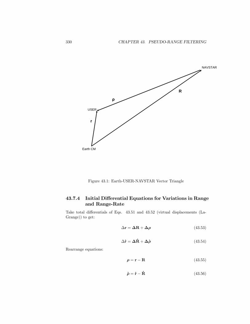
330 CHAPTER 43. PSEUDO-RANGE FILTERING
R
ρ
r
Earth CM
NAVSTAR
USER
Figure 43.1: Earth-USER-NAVSTAR Vector Triangle
43.7.4 Initial Di¤erential Equations for Variations in Rangeand Range-Rate
Take total di¤erentials of Eqs. 43.51 and 43.52 (virtual displacements (La-Grange)) to get:
�r =�R+�� (43.53)
�_r =� _R+�_� (43.54)
Rearrange equations:
� = r�R (43.55)
_� = _r� _R (43.56)

43.7. PARTIAL DERIVATIVES FOR HANU 331
�� =�r��R (43.57)
�_� =�_r�� _R (43.58)
De�ne the instantaneous range � (length of vector �) with:
� =p� � � (43.59)
De�ne the instantaneous unit range vector L with:
� = �L (43.60)
Di¤erentiate with time to get:
_� =_�L+ � _L (43.61)
Also, take total di¤erentials to get:
�� = ��L+��L (43.62)
where _� is the instantaneous range-rate. Then:
� = L � � (43.63)
_� = L � _� (43.64)
because L � L =1 and L � _L = 0. Also:
� _� = � � _� (43.65)
Take total di¤erentials of Eq. 43.65 for:
�� _�+ ��_� = �� � _�+ ��� _�
from which:
��_� = _����+ ��� _���� _� (43.66)
Take total di¤erentials of Eq. 43.63 to get:
�� = L��� (43.67)
because �L� (�L) = 0. Insert Eq. 43.57 into Eq. 43.67 to get:
�� = L��r� L ��R (43.68)
Insert Eqs. 43.68, 43.57, and 43.58 into Eq. 43.66 to show:
��_� = _�� (�r��R)� _� (L��r� L ��R)+����_r�� _R
�

332 CHAPTER 43. PSEUDO-RANGE FILTERING
= ( _�� _�L) ��r+ ���_r� ( _�� _�L) ��R� � �� _R
from which:
�_� = ~� ��r+ L��_r� ~� ��R� L �� _R (43.69)
where:
~� =( _�� _�L) =� (43.70)
Eqs. 43.68 and 43.69 are my initial vector di¤erential equations for variationsin instantaneous range and range-rate.
43.7.5 Position and Velocity Variations in Inertial Com-ponent Matrices
Let x and X denote the 3�1 matrices of inertial components of the USER posi-tion vector r and NAVSTAR position vector R. Let [i] denote the conventional3�1 matrix of orthonormal inertial vectors. Then:
L = LT [i] (43.71)
~� = ~�T [i] (43.72)
�r = [i]T�x (43.73)
�_r = [i]T� _x (43.74)
�R = [i]T�X (43.75)
� _R = [i]T� _X (43.76)
43.7.6 Partials
Insert Eqs. 43.73, 43.74, 43.75, 43.76, 43.71, and 43.72 into Eqs. 43.68 and43.69 to get:
�� =�LT��x+
��LT
��X (43.77)
�_� =�~�T��x+
�LT�� _x+
��~�T
��X +
��LT
�� _X (43.78)
The above two expressions are complete due to use of total di¤erentials. For-mally:

43.7. PARTIAL DERIVATIVES FOR HANU 333
�� =
�@�
@x
��x+
�@�
@ _x
�� _x+
�@�
@X
��X +
�@�
@ _X
�� _X (43.79)
�_� =
�@ _�
@x
��x+
�@ _�
@ _x
�� _x+
�@ _�
@X
��X +
�@ _�
@ _X
�� _X (43.80)
Compare terms to derive the desired 1x3 matrices of partial derivative Jacobians:
@�
@x= LT , range with respect to USER position (43.81)
@�
@ _x= 01x3, range with respect to USER velocity (43.82)
@ _�
@x= ~�T , range-rate with respect to USER position (43.83)
@ _�
@ _x= LT , range-rate with respect to USER velocity (43.84)
@�
@�= c, range with respect to USER clock phase (light speed) (43.85)
@�
@ _�= 0, range with respect to USER clock drift (43.86)
@ _�
@�= 0, range-rate with respect to USER clock phase (43.87)
@ _�
@ _�= 1, range-rate with respect to USER clock drift (43.88)
@�
@X= �LT , range with respect to NAVSTAR position (43.89)
@�
@ _X= 01x3, range with respect to NAVSTAR velocity (43.90)
@ _�
@X= �~�T , range-rate with respect to NAVSTAR position (43.91)
@ _�
@ _X= �LT , range-rate with respect to NAVSTAR velocity (43.92)
where ~�T is the 1x3 row matrix of inertial components of vector ~� =( _�� _�L) =�.The subset of partials referred to the USER position and velocity may be checkedagainst those given by Koskela (page 138). The NAVSTAR partials could havebeen derived from the USER partials by skew-symmetry. But we feel moresecure to explicitly derive them all.

334 CHAPTER 43. PSEUDO-RANGE FILTERING

Chapter 44
GPS Carrier Phase Count
44.1 Introduction
My purpose here is to derive and present:
� a representation for the GPS Doppler phase count measurement for ageneric USER spacecraft GPS receiver
� instructions for implementation of GPS Doppler phase count measure-ments
� state parameters to be estimated
� expressions for required partial derivatives
Optimal orbit determination requires the identi�cation and estimation of allobservable unknown serially-correlated stochastic variables. The USER space-craft GPS receiver clock produces an observable unknown serially-correlated sto-chastic variable; viz, the frequency random walk variable identi�ed by Allan[1].Eqs. 44.11, 44.12, and 44.13 explicitly de�ne this variable �fUn , and its rela-tion to the GPS Doppler phase count measurement representation. An explicitrepresentation of �fUn is required for phase count measurement simulation, forsequential �lter design, for construction and analysis of a measurement �rstdi¤erence model, and for the associated optimal orbit determination from realdata.Eqs. 44.72 and 44.73, together with the sequence of bullets that follow,
present the frequency dependent Doppler phase count measurement representa-tion Nni
j for a particular USER-NAVSTAR pair. These equations are inclusiveof an ionosphere model, rigorously derived, that requires the evaluation of TECat beginning and end of the phase count time interval.Eq. 44.86 de�nes construction of the ionosphere-free measurement NEi
j , andits proof follows immediately. The single di¤erence �NE
j de�ned by Eq. 44.118is shown to cancel all USER clock e¤ects.
335

336 CHAPTER 44. GPS CARRIER PHASE COUNT
44.1.1 BlackJack GPS Receiver
Cal Tech�s BlackJack GPS receiver1 recovers a modi�ed form of both L1 P-code(P1) and L2 P-code (P2) ranging2 , in addition to C/A ranging, and providescarrier phase-count measurements on L1, L2, and C/A. According to Kerric Hill(Bruce Haines (JPL)):
� The BlackJack clock frequency is steered so that its phase is always within1�s of GPS time.
� The BlackJack GPS receiver does not provide P1 and P2 pseudo-rangemeasurements directly, but rather, provides measurements that have been"smoothed" using the phase count measurements.
We are not in possession of the BlackJack clock frequency steering algo-rithm. Unfortunately, all measurements are corrupted by the frequency steering.Constructed �rst di¤erence measurements, referred to distinct NAVSTARs, arerequired to remove the e¤ects of USER BlackJack clock frequency steering onboth range and phase count measurements.The BlackJack pseudo-range measurements are signi�cantly improved due to
phase count measurement "polynomial smoothing"; i.e., the BlackJack P1 andP2 pseudo-range measurements are superpositions of pseudo-range and phasecount Doppler. But this generates a problem for those who would process bothsets of measurements: Pseudo-range "measurements" are correlated with thephase count measurements, and this destroys the ability to model their statisticsappropriately. A Hofmann-Wellenhof et. al. smoothing algorithm is presentedat http://www.gmat.unsw.edu.au/snap/gps/gps_survey/chap6/6411.htm. Wecannot con�rm that this is the BlackJack algorithm.
44.2 Implementation
44.2.1 Estimation of Clock Parameters
The sampled frequency sequence of every clock contains both additive whitenoise and additive random walk sequences. The generalized integrals INij andIUij de�ned by Eqs. 44.27 and 44.28 contain both integral white noise (randomwalk) and integral random walk sequences. Thus the sampled phase sequence ofevery clock contains both random walk and integral random walk sequences. Inaddition, the sampled phase sequence of every clock contains a �icker noise se-quence. Flicker noise is important for NAVSTAR atomic clocks, but is relativelyunimportant for USER crystal clocks.An option is required to estimate two clock parameters, phase and frequency,
for each NAVSTAR clock with every GPS measurement combination. An op-tion is required to estimate two clock parameters, phase and frequecy, for each
1BlackJack is available commercially from Spectrum Astro.2US Patent 6,061,390, CIT, Meehan, Thomas, Brooks, Young, and Lawrence, May 9, 2000.

44.3. NOTATION 337
USER spacecraft when single measurement di¤erencing is not used. The exist-ing stochastic crystal clock model is to be used for both NAVSTAR clocks andUSER clocks. A �icker noise model will be added later for NAVSTAR atomicclocks. Estimate random walk and integral random walk sequences in phaseaccording to Eqs. 44.172 through 44.175 in the �lter implementation.
44.2.2 L1 Phase Count Measurements
Eq. 44.73 presents the frequency-dependent NAVSTAR-dependent Dopplerphase count representation Nni
j in �nal form, at time tag tj .
44.2.3 L1, L2 Phase Count Measurements
Remove Ionosphere Perturbations
The Doppler phase count measurement representation NEij over [tj ��t; tj ] is
given by Eq. 44.86, where is de�ned by Eq. ??. This measurement repre-sentation combines the two phase-count measurements N1i
j and N2ij to remove
�rst order ionosphere e¤ects. USER clock e¤ects and NAVSTAR clock e¤ectsremain.
Single Di¤erenced Phase Count Measurements
Given simultaneous phase count measurements NEpj and NEq
j on independentreceiver channels, where p and q refer to distinct NAVSTARS, they can bedi¤erenced to form �NE
j = NEpj �NEq
j , according to Eq. 44.118. The derivedmeasurement �NE
j is then free of all USER clock e¤ects, as demonstrated.
44.2.4 Partial Derivatives
See Section 44.4.7 for orbit partials, and Section 44.10 for non-orbit partials.The phase count measurement has a range di¤erence representation, so partialsof phase count with respect to position and velocity are reduced to the di¤erenceof partials of range with respect to position and velocity.
44.3 Notation
44.3.1 Time
Proper Time � refers to the phase of some clock, or to the mean phase of anensemble of clocks. Coordinate Time t is the fourth relativistic coordinate,where the �rst three coordinates are used to denote a clock position referred toan inertial frame. Proper time and coordinate time are related approximatelywith the di¤erential equation:

338 CHAPTER 44. GPS CARRIER PHASE COUNT
d� = dt
s1�
�2�
c2r+_s2
c2
�(44.1)
derived from the Schwarzschild metric, where � refers to the two-body geocentricgravitational constant, r and _s are spacecraft position and velocity magnitudes,and c is the speed of light in vaccua. Proper Time is associated with clocks,and Coordinate Time is associated with spacecraft position and velocity. Eq.44.1 provides the bridge. Given an epoch, say t0, where the relation between�0 and t0 is estimated or otherwise known, then Eq. 44.1 can be integrated topropagate the relation.
44.3.2 Oscillator and Clock
Every clock is an artifact with two parts, an oscillator and a counter of oscil-lations or phase referred an origin. Some clocks employ "gears" to transformphase count to hours, minutes, and seconds.The TAI (International Atomic Time) second is de�ned: 1 secTAI = 9; 192; 631; 770
cycles3 between two hyper�ne levels of the ground state of cesium at geoid meansea level. The number of seconds after any origin refers to an associated numberof oscillator cycles after that origin. So time refers to the accumulated phase(number of cycles) of a clock.The phase of one oscillator can be physically compared and di¤erenced with
that of another oscillator. Phase is physically measurable only in this sense,but frequency is not physically measureable in any sense. Frequency is derivedby calculating the change in phase with time, where time is the phase of anindependent clock.
44.3.3 Generalized Integral
Stochastic sequences cannot be di¤erentiated4 or integrated, but they can bedi¤erenced and summed. We will refer to these di¤erences and sums as gener-alized derivatives and generalized integrals5 , or just derivatives and integrals.
44.3.4 Doppler Phase Count
The symbol Nnij denotes the Doppler phase count measurement representation:
� referred to the USER spacecraft oscillator
� over time interval [tj ��t; tj ]
� with time tag at tj3The mean value from an ensemble of oscillators is used.4By de�nition, the derivative requires application of a limit that does not exist for stochastic
sequences.5My use of generalized integral is conventional.

44.3. NOTATION 339
� on L-BAND frequency Ln, n 2 f1; 2g
� for NAVSTAR i, i 2 f1; 2; : : : ; 27g
Nnij is inclusive of:
� an integral on Doppler frequency
� an integral on random USER clock e¤ects
� an integral on random NAVSTAR clock e¤ects
� USER receiver PLL (Phase Lock Loop) thermal noise
� ionospheric e¤ects
When there is no need to identify frequency fn or NAVSTAR i, we shallreplace Nni
j with Nj .
44.3.5 Two Types of Phase Count Error
We are interested here in distinguishing phase count measurement errors ac-cording to two types.
Type 1 Error
Let us denote a Type 1 error in Nk with random variable �N (1)k , for k 2
f1; 2; 3; : : :g. According to Kaplan[49], Type 1 errors are dominated by ther-mal noise. Then Type 1 errors are dominantly Gaussian white noise6 , are notobservable from Doppler phase count measurements, cannot be estimated, butmust be accounted for statisically in the sequential �lter for orbit determination.
Type 2 Error
Let us denote a Type 2 error in Nk with random variable �N (2)k , for k 2
f1; 2; 3; : : :g. Let us denote USER receiver clock time with tj , and USER receiverclock timing error with random variable �tk, for k 2 f1; 2; 3; : : :g.De�ne:
�N(2)k = fk�tk (44.2)
Both �tk and �N(2)k are composed of sequences in random walk and integral
random walk. Hence they are serially correlated. Therefore the observable partof �N (2)
k must be estimated and removed.
6All thermal noise is Gaussian and white[15].

340 CHAPTER 44. GPS CARRIER PHASE COUNT
44.4 Receiver Doppler Algorithm
44.4.1 NAVSTAR Frequencies
Nominal GPS NAVSTAR L-BAND frequencies �fNn , n 2 f1; 2g, are de�ned by:
L1 : �fN1 = (154) �fN0 (44.3)
L2 : �fN2 = (120) �fN0 (44.4)
where7 :
�fN0 = (10:23 MHz)�1� 4:4647� 10�10
�(44.5)
The transmitter on each GPS NAVSTAR emits radio signals:
fN1 = �fN1 + �fN1 = (154) fN0 (44.6)
fN2 = �fN2 + �fN2 = (120) fN0 (44.7)
where:
fN0 = �fN0 + �fN0 (44.8)
�fN1 = (154) �fN0 (44.9)
�fN2 = (120) �fN0 (44.10)
where fN0 is generated by the NAVSTAR oscillator, and where �fN0 is a randomperturbation on the nominal frequency �fN0 .
44.4.2 Doppler Frequency
A USER spacecraft receives a Doppler shifted NAVSTAR signal, contaminatedby additive ionospheric e¤ects, with frequency8 �ijf
Nn + �f IONn , where �ij and
�f IONn denote Doppler shift and ionospheric e¤ect. This is subtracted9 fromfrequency fUn , generated by the USER spacecraft oscillator, to de�ne the in-stantaneous Doppler frequency fDn :
7The perturbation is de�ned such that a ground receiver will believe that the fundamentalfrequency f0 = 10:23 MHz.
8The received carrier frequency is not directly measured. Rather, the GPS receiver mea-sures phase, and derives frequency as the change in phase with time, according to the USERclock. The phase measurement is performed using closed-loop feedback control systems, re-ferred to as frequency locked loop (FLL) and Costas Phase Locked Loop (PLL). On signalacquisition[49], an FLL is employed with carrier tracking loop bandwidth wide, followed by aPLL with carrier tracking loop bandwidth as narrow as possible.
9The subtraction order is de�ned by each actual receiver, and so my representation heremay need a sign change for some receivers.

44.4. RECEIVER DOPPLER ALGORITHM 341
fDn = fUn ���ijf
Nn + �f IONn
�(44.11)
NAVSTAR clock phenomenology is embedded in fNn , and USER clock phe-nomenology is embedded in fUn . USER clock phenomenology is assumed todominate NAVSTAR clock phenomenology. Then the di¤erence
�fUn � fNn
�,
captures USER clock phenomenology most signi�cantly:
�fUn = fUn � fNn (44.12)
Solve Eq. 44.12 for fUn , and insert into Eq. 44.11 to get:
fDn = fNn�1� �ij
�+ �fUn � �f IONn (44.13)
Eqs. 44.6 and 44.7 can be written:
fNn = �fNn + �fNn (44.14)
where �fNn is known and de�ned by Eqs. 44.3 and 44.4. �fNn is due to unknownNAVSTAR clock phenomenology. Insert Eq. 44.14 into Eq. 44.13 to get:
fDn =��fNn + �fNn
� �1� �ij
�+ �fUn � �f IONn (44.15)
Eq. 44.15 presents the USER clock phenomenology term �fUn unscaled bythe Doppler shift �ij , and the NAVSTAR clock phenomenology �fNn scaledby�1� �ij
�. The product �fNn
�1� �ij
�is a very complicated random function
of time. The random frequency scalar �f on every clock has two signi�cantadditive components, white noise and random walk.
44.4.3 De�ne Phase Count
Positive zero crossings (cycles) of fDn are counted and accumulated (integrated)by the USER receiver, inclusive of a partial cycle, across a USER de�ned phasecount interval10 [tj ��t; tj ], to construct a rational phase count number Nni
j ,time-tag tj for j 2 f1; 2; : : :g, NAVSTAR i 2 f1; 2; : : : ; 27g. Nni
j consists ofthe sum of an integer number of cycles and a partial cycle. The GPS receiverCostas Phase Lock Loop (PLL) incurs thermal noise[49] �Nni
j , independent foreach NAVSTAR link i. Thus Nni
j has the representation with the generalizedintegral:
Nnij =
Z tj
tj��tfDn dt+ �N
nij (44.16)
When fDn has units cycles/s, and t has units s, then Nnij has units cycles.
10 tj is a relativistic coordinate time; e.g., TCG or GPS Time.

342 CHAPTER 44. GPS CARRIER PHASE COUNT
Begin
Questions:
� Are thermal noise phase components �N1ij and �N2i
j frequency dependent?
� Does there exist �N0j in the GPS receiver such that we can write:
�N1ij = 154 �N0
j
�N2ij = 120 �N0
j
where in the NAVSTAR GPS transmitter we know:
fN1 = (154) fN0
fN2 = (120) fN0
End
44.4.4 Doppler Shift
Consider an L-BAND wave front emitted from a NAVSTAR spacecraft at timeti and received by the USER spacecraft at time tj > ti. The unitless Dopplershift � can be approximated11 to order O
�c�3�with:
�ij = 1�1
c_�ij +
�
c2
�1
rj� 1
Ri
�+
1
2c2
h_s2j � _S2i
i(44.17)
where:
� c is speed of light in vaccua
� � is the geocentric two-body gravitational constant
� rj and _sj are magnitudes of USER spacecraft position and velocity vectorsat time tj
� Ri and _Si are magnitudes of NAVSTAR spacecraft position and velocityvectors at time ti
� _�ij is the range-rate _�ij = d�ij=dt at time t = tj
� �ij is the range between NAVSTAR spacecraft at time ti and USER space-craft at time tj
11This approximation derives from the use of the Schwarzschild metric, derived from Eq. ??.Appendix D herein provides a derivation of this expression, given the Schwarzschild metric.

44.4. RECEIVER DOPPLER ALGORITHM 343
Approximately: Z tj
tj��t_�ijdt = �ij (tj)� �ij (tj ��t) (44.18)
De�ne:
��ij = �ij (tj)� �ij (tj ��t) (44.19)
�ij =
Z tj
tj��t
��
c2
�1
rj� 1
Ri
�+
1
2c2
h_s2j � _S2i
i�dt (44.20)
�ij = ��ij=c� �ij (44.21)
where ��ij has distance units, �ij has time units, and �ij has time units. Then:
�ij =
Z tj
tj��t(1� �) dt (44.22)
Relativity
Eq. 44.17 has two relativistic terms: �c2
h1rj� 1
Ri
iis due to general relativity and
12c2
h_s2j � _S2i
iis due to special relativity. This is important for one-way Doppler
measurements. Position magnitudes Ri and rj refer to NAVSTAR and USER
spacecraft clock positions. Since Ri 6= rj , then�c2
h1rj� 1
Ri
imust be modeled.
Velocity magnitudes _Si and _sj refer to NAVSTAR and USER spacecraft clock
inertial speeds. Since _Si 6= _sj , then 12c2
h_s2j � _S2i
imust be modeled. On the
other hand, if the same ground-�xed clock is used for transmitter and receiverin a two-way Doppler measurement, then Ri = rj and _Si = _sj , and relativityvanishes.
44.4.5 Phase Count Representation
Insert Eq. 44.15 into Eq. 44.16 to get:
Nnij =
Z tj
tj��t
���fNn + �fNn
� �1� �ij
�+ �fUn � �f IONn
�dt+ �Nni
j (44.23)
The nominal frequency �fNn is a time constant. Then:
Nnij = �fNn
Z tj
tj��t
�1� �ij
�dt+
Z tj
tj��t�fNn
�1� �ij
�dt+
Z tj
tj��t�fUn dt�
Z tj
tj��t�f IONn dt+�Nni
j
(44.24)

344 CHAPTER 44. GPS CARRIER PHASE COUNT
Let us denote clock phase phenomenology of NAVSTAR and USER clocks withInNij and IUj , with time-tags tj , where I
nNij is referred to NAVSTAR i. De�ne
InNij and IUj with:
Z tj
tj��t�fNn
�1� �ij
�dt = �fNn
Z tj
tj��t
��fNn�fNn
� �1� �ij
�dt = �fNn I
nNij (44.25)
Z tj
tj��t�fUn dt =
�fUn
Z tj
tj��t
��fUn�fUn
�dt = �fUn I
nUj (44.26)
That is:
InNij =
Z tj
tj��t
��fNn�fNn
� �1� �ij
�dt (44.27)
InUj =
Z tj
tj��t
��fUn�fUn
�dt (44.28)
where �fNn = �fNn and �fUn = �f
Un are fractional frequencies on NAVSTAR and USER
clocks. Eq. 44.24 becomes:
Nnij = �fNn
Z tj
tj��t
�1� �ij
�dt+ �fNn I
nNij + �fUn I
nUj �
Z tj
tj��t�f IONn dt+ �Nni
j
(44.29)Insert Eq. 44.22 into Eq. 44.29:
Nnij = �fNn �ij +
�fNn InNij + �fUn I
nUj �
Z tj
tj��t�f IONn dt+ �Nni
j (44.30)
44.4.6 Approximations for �ijThe integral for Eq. 44.20 can be approximated. De�ne:
� =�
c2
�1
rj� 1
Ri
�+
1
2c2
h_s2j � _S2i
i(44.31)
�USER =�
c2rj+
_s2j2c2
(44.32)
�NAV =�
c2Ri+
_S2i2c2
(44.33)
Then:
� = �USER + �NAV (44.34)

44.4. RECEIVER DOPPLER ALGORITHM 345
De�ne:
�USERij =
Z tj
tj��t
(�
c2rj+
_s2j2c2
)dt (44.35)
�NAVij = �Z tj
tj��t
(�
c2Ri+
_S2i2c2
)dt (44.36)
Then:
�ij = �USERij + �NAVij (44.37)
Use the symbol over-bar to denote mean values: ��USER, ��NAV , ��, ��USERij ,��NAVij , and ��ij . Then:
�� = ��USER + ��NAV (44.38)
��ij = ��USERij + ��NAVij (44.39)
NAVSTAR orbits are near circular, so mean values can be used for Ri, _Si, �NAV
and �NAVij . When USER spacecraft orbits are near circular, mean values for rj ,_sj , �USER, and �USERij can be used. Then from Eq. 44.20:
��ij = ���t (44.40)
When the USER orbit is eccentric, then a running approximation �USERij for�USERij is required to calculate ��ij :
��ij = �USERij + ��NAVij (44.41)
44.4.7 USER Orbit Partial Derivatives
From Eqs. 44.19 and 44.21:
�ij =��ij (tj)� �ij (tj ��t)
�=c� �ij (44.42)
where �ij has time tag-tag at tj . Di¤erentiate �ij with respect to z and _z, theUSER spacecraft position and velocity 3� 1 component matrices:
@�ij@zj
=@�ij (tj)
@zj�@�ij (tj ��t)
@zj�@�ij@zj
(44.43)
@�ij@ _zj
=@�ij (tj)
@ _zj�@�ij (tj ��t)
@ _zj�@�ij@ _zj
(44.44)
where @�ij=@zj and @�ij=@ _zj are 1� 3 matrices, and where:

346 CHAPTER 44. GPS CARRIER PHASE COUNT
@�ij (tj ��t)@zj
=@�ij (tj ��t)@z (tj ��t)
@z (tj ��t)@z (tj)
(44.45)
@�ij (tj ��t)@ _zj
=@�ij (tj ��t)@ _z (tj ��t)
@ _z (tj ��t)@ _z (tj)
(44.46)
The transition matrix � (tj ��t; tj) on Z = (z; _z)T has the form:
� (tj ��t; tj) ="
@z(tj��t)@z(tj)
@z(tj��t)@ _z(tj)
@ _z(tj��t)@z(tj)
@ _z(tj��t)@ _z(tj)
#(44.47)
so calculate � (tj ��t; tj), then extract @z (tj ��t) =@z (tj) and @ _z (tj ��t) =@ _z (tj)as needed. The range partials algorithm is available from the GPS range algo-rithm document. The �ij partials can probably be ignored due to their deweight-ing by c�2:
@�ij@zj
=
Z tj
tj��t
1
c2
(�
"@r�1j@zj
#+1
2
"@ _s2j@zj
#)dt
@�ij@ _zj
=
Z tj
tj��t
1
c2
(�
"@r�1j@ _zj
#+1
2
"@ _s2j@ _zj
#)dt
The 1� 3 matrices of frequency-dependent phase count partial derivatives withrespect to USER position and velocity are calculated with:
@Nnj
@zj=�fUn � �fUn
� @�ij@zj
(44.48)
@Nnj
@ _zj=�fUn � �fUn
� @�ij@ _zj
(44.49)
44.5 Ionosphere
44.5.1 Physics
Let us denote the ionospheric refractive index by nPH , the group refractiveindex by nGD, radio frequency by f , and electron density (units: number ofelectrons/m3) by Ne. From �rst principles[11], it is shown that:
nPH = 1�A�Nef2
�(44.50)
nGD = 1 +A
�Nef2
�(44.51)
where A is de�ned by:

44.5. IONOSPHERE 347
A =e2
8�2�0me(44.52)
with constants:
Symbol Name Constant Valuee electron charge 1:6021892� 10�19C�0 electric permitivity 8:854187818� 10�12F=mme electron mass 10�31kg
Table 44.1: Elements of A
Notation for variables:
� NTEC : total electron content
� �PH : ionospheric phase range
� �GD: ionospheric group delay range
� �tPH : ionospheric phase advance
� �tGD ionospheric group delay
� 'ION : ionospheric phase
From Eq. 44.52:
A = 40:30816�m3Hz2/electron
�(44.53)
44.5.2 Total Electron Content
The total electron content NTEC is the integral of electron density Ne along thepath of the radio signal from transmitter to receiver. NTEC values from groundto spacecraft are bounded[53]: 1016 electrons/m2 < NTEC < 1019 electrons/m2.From Eqs. 44.50 and 44.51:
�PH = �A�NTECf2
�(44.54)
�GD = +A
�NTECf2
�(44.55)
�tPH =�PHc
= �A�NTECcf2
�(44.56)

348 CHAPTER 44. GPS CARRIER PHASE COUNT
�tGD =�GDc
= +A
�NTECcf2
�(44.57)
'ION = f�tPH = �A�NTECcf
�(44.58)
�f ION = d'=dt = ��A
cf
� �dNTECdt
�(44.59)
Ionospheric group delay range �GD, de�ned by Eq. 44.55, is inversely propor-tional to frequency-squared f2. But ionospheric phase delay frequency �f ION ,de�ned by Eq. 44.59, is inversely proportional to frequency f .
Units
Conventionally, there are two sets of units used in the literature for NTEC :Natural units TECN:
TECN =1 electronm2
(44.60)
in which case:
A = 40:30816�(m)(Hz2)/TECN
�(44.61)
and scaled units TECU:
TECU =1� 1016 electrons
m2(44.62)
in which case:
A = 40:30816� 104�(m)(MHz2)/TECU
�(44.63)
where 1 MHz = 1� 106 Hz. Then:
�tGD =�40:30816
�(m)(Hz2)/TECN
���NTECcf2
�(44.64)
�tGD =�40:30816� 104
�(m)(MHz2)/TECU
���NTECcf2
�(44.65)
'ION = ��40:30816
�(m)(Hz2)/TECN
���NTECcf
�(44.66)
'ION = ��40:30816� 104
�(m)(MHz2)/TECU
���NTECcf
�(44.67)

44.6. FINAL FORMS FOR PHASE COUNT 349
�f ION = �
2440:30816�(m)(Hz2)/TECN
�cf
35�dNTECdt
�(44.68)
�f ION = �
2440:30816� 104�(m)(MHz2)/TECU
�cf
35�dNTECdt
�(44.69)
44.5.3 Validation
Sections 10.8 and 10.9 of The Handbook of Geophysics and the Space Envi-ronment [53], by Klobuchar, presents expressions for comparison. Validate Eq.44.64 by comparison to Klobuchar Eq. 10.70.Insert
�c = 2:99792458� 108 m/s
�into Eq. 44.68 to get:
�f ION = ��1:344536� 10�7
f
�(Hz)(cycles)TECN
���dNTECdt
�(44.70)
If f is evaluated in units Hz and dNTEC=dt is evaluated in units TECN/s, then�f IONn will have units Hz. Validate Eq. 44.70 by comparison to Klobuchar Eq.10.78, noting Klobuchar�s sign error.
44.6 Final Forms for Phase Count
Insert Eq. 44.59 into Eq. 44.30 to get:
Nnij = �fNn �ij +
�fNn InNij + �fUn I
nUj +
�A
c �fNn
� Z tj
tj��t
�dNTECdt
�dt+ �Nni
j (44.71)
De�ne:
�NTEC = NTEC (tj)�NTEC (tj ��t) (44.72)
Then Eq. 44.71 becomes:
Nnij = �fNn �ij +
�fNn InNij + �fUn I
nUj +A�NTEC=
�c �fNn
�+ �Nni
j (44.73)
Eq. 44.73 presents the frequency-dependent NAVSTAR-dependent Dopplerphase count representation Nni
j in �nal form, at time tag tj . Terms on theright-hand side can be described:
� �fNn �ij is the deterministic phase e¤ect, where �ij = ��ij=c� �ij , and �ijis the integral of the relativistic expression

350 CHAPTER 44. GPS CARRIER PHASE COUNT
� InUj is the random frequency dependent phase phenomenology in theUSER GPS receiver clock
� InNij is the random frequency dependent phase phenomenology in theNAVSTAR transmitter clock
� A�NTEC=�c �fNn
�is the random frequency dependent ionospheric e¤ect on
phase
� �Nnij is the USER receiver Costas Phase Lock Loop thermal noise, inde-
pendent for each NAVSTAR link i.
44.6.1 Alternate Representation
GPS carrier phase measurements residuals, intrinsically de�ned in units cycles,are frequently expressed in the distance units of range; e.g., centimeters or mil-limeters. There does not exist a mapping from carrier phase to range, but theredoes exist a mapping from carrier phase to range di¤erence. But in so doing,one must be careful to avoid a fundamental change in semantics. Eq. 44.73de�nes the phase measurement Nni
j as a sum of noise-free signal �fNn �ij , clocknoise �fNn I
nNij + �fUn I
nUj , uncertain ionosphere perturbation A�NTEC=
�c �fNn
�,
and thermal noise �Nnij . Eq. 44.75 represents signal component range di¤er-
ence ��ij as a sum of scaled measurement �Nn Nnij , noise-free signal component
c�ij , clock noise �fNn I
nNij + �fUn I
nUj , ionosphere perturbation A�NTEC=
�c �fNn
�,
and thermal noise �Nnij . It is clear that range di¤erence ��ij is a signal compo-
nent of the measurement Nnij , and in no way can be identi�ed as a measurement
�without a fundamental change in semantics.Let �n denote wave length for carrier frequency �fNn . Then:
�n �fNn = c (44.74)
where for L1 and L2:
�1 = 19:029367cmcycle
�2 = 24:42102cmcycle
From Nnij to ��ij
Insert Eqs. 44.74 and 44.21 into Eq. 44.73:
��ij = �Nn Nnij + c�ij � c
�InNij + InUj
�� A�NTEC�
�fNn�2 � �Nn �Nni
j (44.75)
where �ij , de�ned by Eq. 44.20, is the time integral of contributions due tospecial and general relativity, and where we have assumed:

44.7. IONOSPHERE REMOVAL 351
�Nn c
�Un= 1 (44.76)
44.7 Ionosphere Removal
Consider every linear weighted combination:
NEij = aN1i
j + bN2ij (44.77)
to �nd expressions for undetermined unitless constants a and b, such that: (i)NEij is free of the ionospheric term A�NTEC=
�c �fNn
�of Eq. 44.73, and (ii) the
sum Sab of measurement weights a and b is unity:
Sab = a+ b = 1 (44.78)
Insert phase count measurement representations N1ij and N2i
j of Eq. 44.73 intoEq. 44.77 to get:
NEij =
�a �fN1 + b �fN2
��ij+
�A�NTEC
c
��a�fN1+
b�fN2
�+(3 other terms) (44.79)
Set: �a�fN1+
b�fN2
�= 0 (44.80)
to free NEij of the ionospheric term A�NTEC=
�c �fNn
�in Eq. 44.79 and satisfy
the �rst constraint on Eq. 44.77. Then Eqs. 44.80 and 44.78 yield:
b = �� �fN2�fN1
�a (44.81)
and:
Sab =
� �fN1 � �fN2�fN1
�a (44.82)
Then from Eqs. 44.78 and 44.81, expressions for the measurement weights aand b are found:
a =�fN1
�fN1 � �fN2(44.83)
b = ��fN2
�fN1 � �fN2(44.84)
Then from Eq. 44.77:

352 CHAPTER 44. GPS CARRIER PHASE COUNT
NEij =
�fN1 N1ij � �fN2 N
2ij
�fN1 � �fN2(44.85)
or:
NEij =
N1ij �N2i
j
� 1 (44.86)
where:
= �fN1 =�fN2 (44.87)
Refer to NEij as the ionosphere-free carrier-phase measurement. Insert Eq. 44.73
into Eq. 44.86 to get the measurement representation �NEij to be used in the
�lter:
�NEij =
�fN1 H1ij � �fN2 H
2ij
�fN1 � �fN2(44.88)
where ionosphere e¤ects vanish, and where:
Hnij = �fNn �ij + I
nNij + InUj + �Nni
j (44.89)
De�ne:
JnNij = �fNn �ij + InNij + InUj (44.90)
so that:
Hnij = JnNij + �Nni
j (44.91)
Then the ionosphere-free carrier-phase measurement can be written:
�NEij = SNij +WNi
j (44.92)
where the measurement signal SNij is given by:
SNij =�fN1 J
1Nij � �fN2 J
2Nij
�fN1 � �fN2(44.93)
and measurement white noise WNij is given by:
WNij =
�fN1 �N1ij � �fN2 �N
2ij
�fN1 � �fN2(44.94)
De�ne:
F1 =�fN1
�fN1 � �fN2(44.95)
F2 =�fN2
�fN1 � �fN2(44.96)
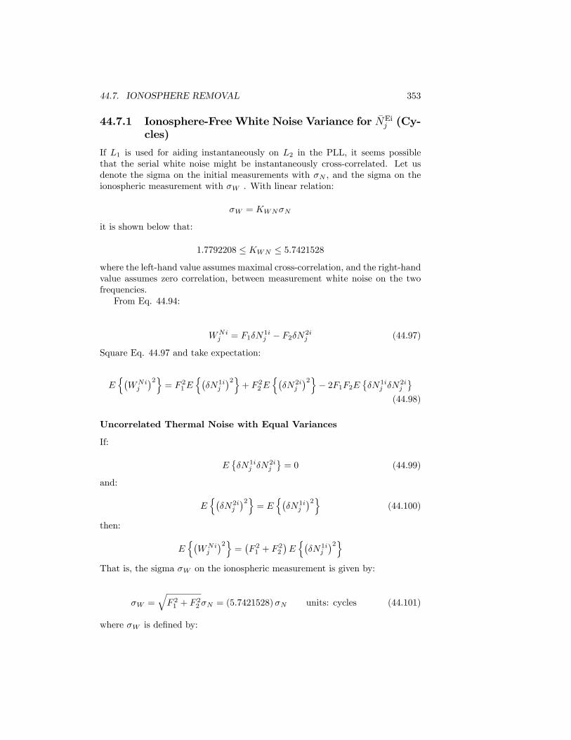
44.7. IONOSPHERE REMOVAL 353
44.7.1 Ionosphere-Free White Noise Variance for �NEij (Cy-
cles)
If L1 is used for aiding instantaneously on L2 in the PLL, it seems possiblethat the serial white noise might be instantaneously cross-correlated. Let usdenote the sigma on the initial measurements with �N , and the sigma on theionospheric measurement with �W . With linear relation:
�W = KWN�N
it is shown below that:
1:7792208 � KWN � 5:7421528
where the left-hand value assumes maximal cross-correlation, and the right-handvalue assumes zero correlation, between measurement white noise on the twofrequencies.From Eq. 44.94:
WNij = F1�N
1ij � F2�N2i
j (44.97)
Square Eq. 44.97 and take expectation:
En�WNij
�2o= F 21E
n��N1i
j
�2o+ F 22E
n��N2i
j
�2o� 2F1F2E ��N1ij �N
2ij
(44.98)
Uncorrelated Thermal Noise with Equal Variances
If:
E��N1i
j �N2ij
= 0 (44.99)
and:
En��N2i
j
�2o= E
n��N1i
j
�2o(44.100)
then:
En�WNij
�2o=�F 21 + F
22
�En��N1i
j
�2oThat is, the sigma �W on the ionospheric measurement is given by:
�W =qF 21 + F
22 �N = (5:7421528)�N units: cycles (44.101)
where �W is de�ned by:

354 CHAPTER 44. GPS CARRIER PHASE COUNT
�W =
rEn�WNij
�2ounits: cycles (44.102)
and where �N , the sigma on the initial measurements, is de�ned by:
�N =
rEn��N1i
j
�2ounits: cycles (44.103)
Correlated Thermal Noise
Assume there exist �N0j in the GPS receiver such that:
�N1ij = 154�N0i
j =
�f1f0
��N0i
j (44.104)
�N2ij = 120�N0i
j =
�f2f0
��N0i
j (44.105)
where in the NAVSTAR GPS transmitter we know:
fN1 = (154) fN0
fN2 = (120) fN0
Then:
�N0ij =
�f0f1
��N1i
j =
�f0f2
��N2i
j
and:
En�WNij
�2o=(f1 + f2)
2
f20En��N0i
j
�2o(44.106)
or:
�W =
�f1 + f2f0
��N0 units: cycles (44.107)
f1 + f2f0
= 274
where:
�W =
rEn�WNij
�2ounits: cycles
�N0 =
rEn��N0i
j
�2ounits: cycles
Since:

44.7. IONOSPHERE REMOVAL 355
�N0ij =
�f0f1
��N1i
j =
�f0f2
��N2i
j
then:
rEn��N0i
j
�2o=
�1
154
�rEn��N1i
j
�2o=
�1
120
�rEn��N2i
j
�2oTherefore:
�W =��N1154
�=��N2120
�units: cycles
where:
�N1 =
rEn��N1i
j
�2ounits: cycles
�N2 =
rEn��N2i
j
�2ounits: cycles
44.7.2 Ionosphere-Free White Noise Variance for �� (cm)
Eq. 44.85 can be written:
NEij =
�2N1ij � �1N2i
j
�2 � �1(44.108)
where �nfn = c. Insert Eq. 44.75 into Eq. 44.108 to get:
��ij = �SNEij +c�ij�c�1
�I1Nij + I1Uj
�+c�2
�I2Nij + I2Uj
���W1�N
1ij +�W2�N
2ij
(44.109)where the wave-length coe¢ cients are de�ned and evaluated:
�W1 =�1�
22
�22 � �21= 48:443594 cm/cycle; thermal noise L1 (44.110)
�W2 =�21�2
�22 � �21= 37:748257 cm/cycle; thermal noise L2 (44.111)
�S =�1�2�2 + �1
= 10:695338 cm/cycle; signal (44.112)
�1 =�22
�22 � �21= 2:5457281 (unitless); clocks L1 (44.113)

356 CHAPTER 44. GPS CARRIER PHASE COUNT
�2 =�21
�22 � �21= 1:5457281 (unitless); clocks L2 (44.114)
and where ionospheric terms subtract out12 . Note that NEij and �ij are de-
terministic signals. Thermal noises �N2ij and �N1i
j are independent of clocknoises InNij and InUj (derived from oscillators) because thermal noise is whitenoise. The sizes of white noise coe¢ cients �W1 = 48:443594 cm/cycle and�W2 = 37:748257 cm/cycle, relative to signal �S = 10:695338 cm/cycle, aresomewhat alarming.De�ne:
W = �W2�N2ij � �W1�N
1ij (44.115)
Then:
E�W 2=
��1�
22
�22 � �21
�2En��N1i
j
�2o+
��21�2
�22 � �21
�2En��N2i
j
�2o
� 2�
�1�22
�22 � �21
���21�2
�22 � �21
�E��N1i
j �N2ij
(44.116)
Uncorrelated Thermal Noise with Equal Variances
If:
E��N1i
j �N2ij
= 0
and:
En��N2i
j
�2o= E
n��N1i
j
�2othen:
E�W 2=��2W1 + �
2W2
�En��N1i
j
�2oand:
�W =q�2W1 + �
2W2�Nq
�2W1 + �2W2 = 61:414271 cm/cycle
where:12The equation above was derived in mid 2004, and then rederived on 21 Mar 05 � with
same result.

44.7. IONOSPHERE REMOVAL 357
�W =pE fW 2g
�N =
rEn��N1i
j
�2oCorrelated Thermal Noise
E�W 2=
��1�
22
�22 � �21
�2En��N1i
j
�2o+
��21�2
�22 � �21
�2En��N2i
j
�2o�2�
�1�22
�22 � �21
���21�2
�22 � �21
�E��N1i
j �N2ij
Now �N1i
j and �N2ij denote thermal noise, in units cycles, on L1 and L2,
and W denotes thermal noise after ionosphere combination in units cm.
W = �W2�N2ij � �W1�N
1ij
= ��ij ���SN
Eij + c�ij � c�1
�I1Nij + I1Uj
�+ c�2
�I2Nij + I2Uj
��N1i
j = 154 �N0j
�N2ij = 120 �N0
j
E�W 2== �20E
n��N0
j
�2oThus:
�W = �0 �N0
where:
�0 = 2930:522 cm/cycle
�W =pE fW 2g
�N0 =
rEn��N0
j
�2oNow:
�0 = 154 �1 = 120 �2

358 CHAPTER 44. GPS CARRIER PHASE COUNT
and:
�N1ij = 154 �N0
j
�N2ij = 120 �N0
j
So:
En��N0
j
�2o=
�1
154
�2En��N1i
j
�2o=
�1
120
�2En��N2i
j
�2oand:
rEn��N0
j
�2o=
�1
154
�rEn��N1i
j
�2o=
�1
120
�rEn��N2i
j
�2o
�N0 =
�1
154
��N1 =
�1
120
��N2
Therefore:
�W = �1�N1 = �2�N2 (44.117)
�W = (19:029367 cm/cycle)�N1 = (24:42102 cm/cycle)�N2
where:
�N1 =
rEn��N1i
j
�2o
�N2 =
rEn��N2i
j
�2o
44.8 First Di¤erences on NEij
44.8.1 Remove USER Clock Phase Perturbations
De�ne:
�NEj = NEp
j �NEqj (44.118)
where p and q refer to distinct NAVSTARS. Insert Eq. 44.88 into Eq. 44.118to get:
��fN1 � �fN2
��NE
j =h�fN1 H
1pj � �fN2 H
2pj
i�h�fN1 H
1qj � �fN2 H
2qj
i(44.119)
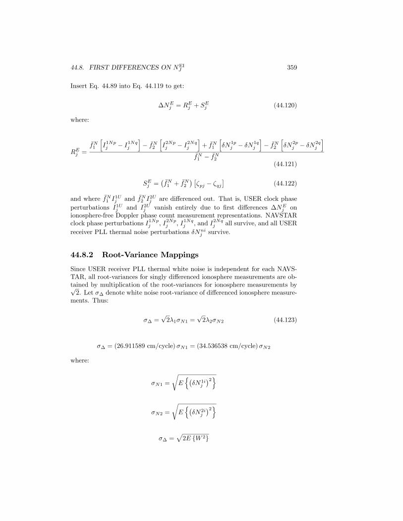
44.8. FIRST DIFFERENCES ON NEIJ 359
Insert Eq. 44.89 into Eq. 44.119 to get:
�NEj = REj + S
Ej (44.120)
where:
REj =
�fN1
hI1Npj � I1Nqj
i� �fN2
hI2Npj � I2Nqj
i+ �fN1
h�N1p
j � �N1qj
i� �fN2
h�N2p
j � �N2qj
i�fN1 � �fN2
(44.121)
SEj =��fN1 + �fN2
� ��pj � �qj
�(44.122)
and where �fN1 I1Uj and �fN2 I
2Uj are di¤erenced out. That is, USER clock phase
perturbations I1Uj and I2Uj vanish entirely due to �rst di¤erences �NEj on
ionosphere-free Doppler phase count measurement representations. NAVSTARclock phase perturbations I1Npj , I2Npj , I1Nqj , and I2Nqj all survive, and all USERreceiver PLL thermal noise perturbations �Nni
j survive.
44.8.2 Root-Variance Mappings
Since USER receiver PLL thermal white noise is independent for each NAVS-TAR, all root-variances for singly di¤erenced ionosphere measurements are ob-tained by multiplication of the root-variances for ionosphere measurements byp2. Let �� denote white noise root-variance of di¤erenced ionosphere measure-
ments. Thus:
�� =p2�1�N1 =
p2�2�N2 (44.123)
�� = (26:911589 cm/cycle)�N1 = (34:536538 cm/cycle)�N2
where:
�N1 =
rEn��N1i
j
�2o
�N2 =
rEn��N2i
j
�2o
�� =p2E fW 2g

360 CHAPTER 44. GPS CARRIER PHASE COUNT
44.9 Example
Suppose:
�� = 1 cm
Then:
�N1 =1 cm
26:911589 cm/cycle= 0:0371587 cycles
�N2 =1 cm
34:536538 cm/cycle= 0:0289548 cycles
44.10 Partials and Covariance
In symmetry with Eqs. 44.5 through 44.10, de�ne:
�fN0 = (10:23 MHz)�1� 4:4647� 10�10
�(44.124)
USER clock frequencies can be su¢ ciently approximated with:
fU1 =�fU1 + �f
U1 = (154) f
U0 (44.125)
fU2 =�fU2 + �f
U2 = (120) f
U0 (44.126)
where:
fU0 =�fU0 + �f
U0 (44.127)
�fU1 = (154) �fU0 (44.128)
�fU2 = (120) �fU0 (44.129)
where fU0 is generated by the USER spacecraft oscillator, and where �fU0 is arandom perturbation on the nominal frequency �fU0 .
44.10.1 Single Frequency
Recall Eq. 44.73:
Nnij =
��fNn + �fNn
��ij + �f
Un �t+ �N
nij +A�NTEC=
�cfNn
�

44.10. PARTIALS AND COVARIANCE 361
Partials
@Nnij
@�fUn= �t (44.130)
@Nnij
@�fNn= �ij (44.131)
Covariance
PNnij= E
n�Nnij
�2o
PNnij=��ij�2En��fNn
�2o+ (�t)
2En��fUn
�2o+ E
n��Nni
j
�2o(44.132)
44.10.2 Two-Frequency Ionosphere Removal
Insert Eqs. 44.125 and 44.126 into Eq. 44.88, and then use Eq. 44.89 and Eqs.44.128 and 44.129 to get:
NEij =
�1
34
�h�(154)
2 � (120)2� ��t�fU0 +
��fN0 + �fN0
��ij�+�(154) �N1i
j � (120) �N2ij
�i(44.133)
Partials
De�ne unitless constant B:
B =
h(154)
2 � (120)2i
(34)= 274 (44.134)
Estimate USER clock frequency perturbation �fU0 :
@NEij
@�fU0= B�t (44.135)
Estimate NAVSTAR clock frequency perturbation �fN0 :
@NEij
@�fN0= B�ij (44.136)

362 CHAPTER 44. GPS CARRIER PHASE COUNT
Covariance
De�ne:
PEi j = En�NEij
�2o(44.137)
Insert Eq. 44.133 into Eq. 44.137. Then:
PEi j = B2 (�t)2En��fU0
�2o+B2�2ijE
n��fN0
�2o
+
�154
34
�2En��N1i
j
�2o+
�120
34
�2En��N2i
j
�2o(44.138)
44.10.3 First Di¤erences on NEij
�NEj =
��fN1 + �fN2
� ��pj � �qj
�+��Ej (44.139)
��Ej =�B��pj � �qj
� ��fN0
�+�WE
j
�(44.140)
�WEj =
�154
34
���N1p
j � �N1qj
���120
34
���N2p
j � �N2qj
�(44.141)
Partials
@�NEj
@�fN0= B
��pj � �qj
�(44.142)
Covariance
En��NE
j
�2o= E
����Ej
�2�(44.143)
E
����Ej
�2�= B2
��pj � �qj
�2En��fN0
�2o+ E
n��WE
j
�2o(44.144)
En��WE
j
�2o=
�154
34
�2 �E
���N1p
j
�2�+ E
���N1q
j
�2��
+
�120
34
�2 �E
���N2p
j
�2�+ E
���N2q
j
�2��(44.145)

44.11. RECEIVER CLOCK ERROR MODEL 363
44.11 Receiver Clock Error Model
We shall assume that the receiver clock is a state-of-the-art oven-controlledcrystal clock.AGI resources have been applied to simulate and graph appropriate ensem-
bles of clock modeling stochastic sequences in clock phase xj and fractional fre-quency �yj , and overlay the graphs with associated two-sigma boundary curves.Mutual validation of simulations and covariance calculations has been achievedwith a demonstration of consistency between an ensemble of simulations and itstwo-sigma boundaries.
44.11.1 Covariance on Clock Phase
Our physical clock model derives from Allan[1], Table II, page 651. Values forclock dependent parameter constants a0 and a�2 de�ne selected models for com-position of the Allan variance �2y (�) according to Eqs. 44.151 and 44.154. Weassume that the receiver clock can be su¢ ciently characterized13 by frequencymodulated (FM) white noise and frequency modulated random walk. Thenclock phase modulation (PM) will be driven by their generalized integrals.Let x (t) denote clock time deviation (or clock phase deviation) and let y (t)
denote clock frequency deviation. Formally, Allan[1] presents the (generalized14)integral:
x (t) =
Z t
0
y (�) d� (44.146)
Let � denote clock sample time. The sample Allan variance is de�ned by:
�2y (�) = limn!1
1
2n
nXj=1
(�yj+1 � �yj)2 (44.147)
where:
�yj =xj+1 � xj
�(44.148)
� = tj+1 � tj (44.149)
xj = x (tj) (44.150)
13This assumption is supported by Allan: "Note that the quadratic D term occurs becausex (t) is the integral of y (t), the fractional frequency, and is often the predominant cause oftime deviation."14Allan does not distinguish between integrals and generalized integrals in his paper refer-
enced above. But the standard calculus does not work for the "integration" of white noise andrandom walk sequences. These sequences are summable and di¤erenceable, but they are notintegrable and di¤erentiable. It is nonetheless helpful to communicate the relation betweenx and y by analogy to the standard calculus in the absence of measure theory and Lebesgueintegration tools.

364 CHAPTER 44. GPS CARRIER PHASE COUNT
Frequency White Noise
The physical Allan variance for FM white noise is given by:
�2y (�) = a0��1, FM white noise (44.151)
Compare Eqs. 44.147 and 44.151 to write:
a0��1 = lim
n!1
1
2n
nXj=1
(�yj+1 � �yj)2 (44.152)
From this equation derive:
E fx (tk)x (tj)g = (a0) (min [tj ; tk]) (44.153)
A candidate value: a0 = 10�23s.
Frequency Random Walk
The physical Allan variance for FM random walk is given by:
�2y (�) = a�2� , FM random walk (44.154)
Compare Eqs. 44.147 and 44.154 to write:
a�2� = limn!1
1
2n
nXj=1
(�yj+1 � �yj)2 (44.155)
Adopt the reset to zero condition:
yj = 0, tj = 0 (44.156)
Then derive:
En(y (t))
2o= 3a�2t (44.157)
A candidate value: a�2 =�10�25=500
�s�1.
Superposition
Ignoring FM �icker noise and phase modulated (PM) sequences given by Allan,then:
�2y (�) = a0��1 + a�2� (44.158)
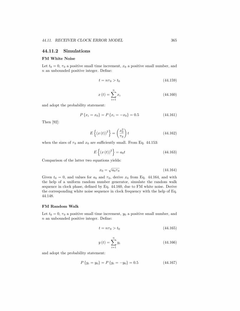
44.11. RECEIVER CLOCK ERROR MODEL 365
44.11.2 Simulations
FM White Noise
Let t0 = 0, �0 a positive small time increment, x0 a positive small number, andn an unbounded positive integer. De�ne:
t = n�0 > t0 (44.159)
x (t) =nXi=1
xi (44.160)
and adopt the probability statement:
P fxi = x0g = P fxi = �x0g = 0:5 (44.161)
Then [92]:
En(x (t))
2o=
�x20�0
�t (44.162)
when the sizes of �0 and x0 are su¢ ciently small. From Eq. 44.153:
En(x (t))
2o= a0t (44.163)
Comparison of the latter two equations yields:
x0 =pa0�0 (44.164)
Given t0 = 0, and values for a0 and �0, derive x0 from Eq. 44.164, and withthe help of a uniform random number generator, simulate the random walksequence in clock phase, de�ned by Eq. 44.160, due to FM white noise. Derivethe corresponding white noise sequence in clock frequency with the help of Eq.44.148.
FM Random Walk
Let t0 = 0, �0 a positive small time increment, y0 a positive small number, andn an unbounded positive integer. De�ne:
t = n�0 > t0 (44.165)
y (t) =nXi=1
yi (44.166)
and adopt the probability statement:
P fyi = y0g = P fyi = �y0g = 0:5 (44.167)
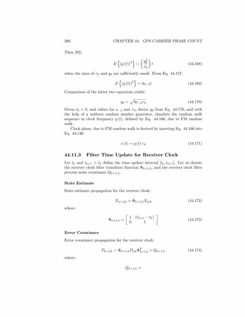
366 CHAPTER 44. GPS CARRIER PHASE COUNT
Then [92]:
En(y (t))
2o=
�y20�0
�t (44.168)
when the sizes of �0 and y0 are su¢ ciently small. From Eq. 44.157:
En(y (t))
2o= 3a�2t (44.169)
Comparison of the latter two equations yields:
y0 =p3a�2�0 (44.170)
Given t0 = 0, and values for a�2 and �0, derive y0 from Eq. 44.170, and withthe help of a uniform random number generator, simulate the random walksequence in clock frequency y (t), de�ned by Eq. 44.166, due to FM randomwalk.Clock phase, due to FM random walk is derived by inserting Eq. 44.166 into
Eq. 44.146:
x (t) = y (t) �0 (44.171)
44.11.3 Filter Time Update for Receiver Clock
Let tk and tk+1 > tk de�ne the time update interval [tk; tk+1]. Let us denotethe receiver clock �lter transition function �k+1;k, and the receiver clock �lterprocess noise covariance Qk+1;k.
State Estimate
State estimate propagation for the receiver clock:
Xk+1jk = �k+1;kXkjk (44.172)
where:
�k+1;k =
�1 (tk+1 � tk)0 1
�(44.173)
Error Covariance
Error covariance propagation for the receiver clock:
Pk+1jk = �k+1;kPkjk�Tk+1;k +Qk+1;k (44.174)
where:
Qk+1;k =

44.11. RECEIVER CLOCK ERROR MODEL 367
�a0 (tk+1 � tk) + a�2 (tk+1 � tk)3 3a�2 (tk+1 � tk)2 =2
3a�2 (tk+1 � tk)2 =2 3a�2 (tk+1 � tk)
�(44.175)
Pjjk =
"P xjjk P xyjjkP yxjjk P yjjk
#, j 2 fk; k + 1g (44.176)
44.11.4 State Estimate Parameters
We shall estimate the fractional frequency y (t) and its generalized integral x (t)for the user spacecraft clock.

368 CHAPTER 44. GPS CARRIER PHASE COUNT

Chapter 45
GPS Navigation Solution
45.1 Introduction
ODTK can convert GPS pseudorange observations into so-called "navigationsolutions." A navigation solution is the estimated position and clock o¤set of aGPS receiver based on four (4) or more pseudoranges at a single epoch. The nav-igation solutions of the USER spacecraft receiver can be used as an alternativemeasurement type and are akin to "normal places" for GPS measurements. Ad-vantages of navigation solutions are that they are faster and simpler to processfor orbit determination purposes; disadvantages are that some information maybe inherently lost as a result of the combination and their observational uncer-tainty may be harder to characterize.Bancroft [4] introduced an analytic method of navigation solution that pro-
vides position and clock o¤set given four (4) pseudoranges at the same time.Yang and Chen [131] provided an extension to Bancroft�s method so that morethan four pseudoranges may be used. This latter algorithm has been adoptedfor use in ODTK.
45.2 Algorithm
Let n � 4 be the number of GPS space-vehicle transmitters observed at the timeof the navigation solution. Let B be a matrix having four columns and n rows.Let the �rst three elements of each row of B contain the position of the ith GPSspace vehicle, and let the fourth element contain the corrected pseudorange �i(c.f. Eq. (43.1)) corresponding with the ith space vehicle, e.g.,
B =
2666664x1 y1 z1 �1x2 y2 z2 �2x3 y3 z3 �3...
......
...xn yn zn �n
3777775 . (45.1)
369

370 CHAPTER 45. GPS NAVIGATION SOLUTION
De�ne the M matrix as
M =
26641 0 0 00 1 0 00 0 1 00 0 0 �1
3775 (45.2)
and generally de�ne the Lorentz inner product for two 4-space vectors a and bas
ha; bi = aTMb = a1b1 + a2b2 + a3b3 � a4b4. (45.3)
Let the USER location and ranging bias of the receiver be represented bythe column vector r =
�x y z c�t
�T, where c is the speed of light and �t
is the receiver clock o¤set relative to GPS system time. The navigation solutionis therefore computed as
r =MB-1 (�� + �) , (45.4)
where � =�1 1 1 � � � 1
�Tis a column vector of length n. Each element
of the vector � is computed from the Lorentz inner product (Eq. (45.3)) of eachof the 4-space row vectors in B (Eq. 45.1) with itself, such that
� =1
2
2666664x1x1 + y1y1 + z1z1 � �1�1x2x2 + y2y2 + z2z2 � �2�2x3x3 + y3y3 + z3z3 � �3�3
...xnxn + ynyn + znzn � �n�n
3777775 . (45.5)
Finally, the scalar � in Eq. 45.4 is a root of the quadratic equation
0 = E�2 + 2F� +G, (45.6)
where
E =D�BTB
�-1BT� ;
�BTB
�-1BT�
E, (45.7)
F =D�BTB
�-1BT� ;
�BTB
�-1BT�
E� 1, (45.8)
G =D�BTB
�-1BT�;
�BTB
�-1BT�
E(45.9)
The solution of � is therefore
� =�F �
pF 2 � 4EG2E
, (45.10)
However, only one of the two roots results in a correct location. Presently,ODTK chooses the root that minimizes the magnitude of the computed clocko¤set, i.e., j�tj.

45.2. ALGORITHM 371
A detailed explanation and justi�cation of the methodology can be found in[4] and [131].

372 CHAPTER 45. GPS NAVIGATION SOLUTION

Part XII
Global Positioning System(GPS) Ground Receivers
373


Chapter 46
GPS Composite Clock
46.1 GOMA-E
The GPS Composite Clock Model has been implemented in ODTK accordingto GOMA-E[109], Section 10.3.2.3.5.10. The GPS clock steering algorithm hasbeen implemented in ODTK according to GOMA-E, Section 10.3.2.3.5.11. Dis-tribution of GOMA-E is authorized for US DOD and its contractors only.The Zucca-Tavella[104] three-state clock model was used in place of the two-
state model referenced in GOMA-E.
46.2 Tutorial
The GPS Composite Clock model derives from a paper by Kenneth Brown[10].This paper is very di¢ cult to read. Therefore I have prepared a tutorial, derivedfrom simulations, to aid in understanding the GPS Composite Clock.
46.2.1 Simulation Narrative
Simulate Random Clock Deviations
First three random clock parameter deviation functionals were simulated foreach of four clocks across an eight-day interval using the Zucca-Tavella[104]clock model. This simulation embedded the evaluation of Wiener processes andthe evaluation of stochastic integrals on Wiener process di¤erentials accordingto Zucca-Tavella.See Fig. 46.1 for an overlay of simulations of clock phase deviations for the
four clocks. Clocks S1 and S2 are GPS ground station clocks, and clocks N1and N2 are spaceborne GPS NAVSTAR clocks.
375

376 CHAPTER 46. GPS COMPOSITE CLOCK
Simulate GPS Range Measurements
Then GPS range1 measurements were simulated using the simulated randomclock phase2 deviation functionals.
Estimate Random Clock Deviations with KF1
I estimated the three random clock parameter deviation functionals from simu-lated GPS range measurements for each of the four clocks using a Kalman �lter,call it KF1, with a 12 � 1 matrix clock state estimate structure. Also, I simu-lated �lter initial condition errors. See Fig. 46.2 for an overlay of simulated andestimated phase deviation functionals for the four clocks. Visual inspection ofFig. 46.2 reveals simulated and estimated phase deviation patterns with de�nitesymmetries.The clock parameter deviation functionals are not observable from the GPS
range measurements �after �lter initialization. That is, the error variance oneach clock parameter deviation is never reduced due to processing a GPS rangemeasurement �after �lter initialization. See Fig. 46.5 for a demonstration ofnon-observability and unboundedness of clock phase deviation for clock S1, andnotice that the phase deviation estimate is consistent with its error covariance.Related graphs for the other three clocks present the same behavior.
Form Clock Variations
I formed di¤erence time functionals by subtracting the estimated clock para-meter deviation functionals from the simulated clock parameter deviation func-tionals. I refer to these di¤erences as clock parameter variations.
46.2.2 Similarity in Clock Parameter Variations
A remarkable phenomenum is observed: The clock parameter variations of eachclock are similar to those of all other clocks in:
� phase
� frequency
� frequency drift
See Figs. 46.3 and 46.4 for a demonstration of clock phase variation similaritywith �lter initial condition errors simulated. Identify each of the four clockparameter variations as an estimate of the Unobserved Variation Commonto all Clocks �the UVCC3 . The Kalman �lter KF1, applied to simulated GPSrange measurements, has enabled the calculation of four estimates of the UVCC.
1 I use GPS range for GPS pseudo-range for clarity in the sequel.2Phase deviation is the �rst of the three random clock parameter deviations.3Ken Brown[10] refers to the UVCC as the Implicit Ensemble Mean (IEM).
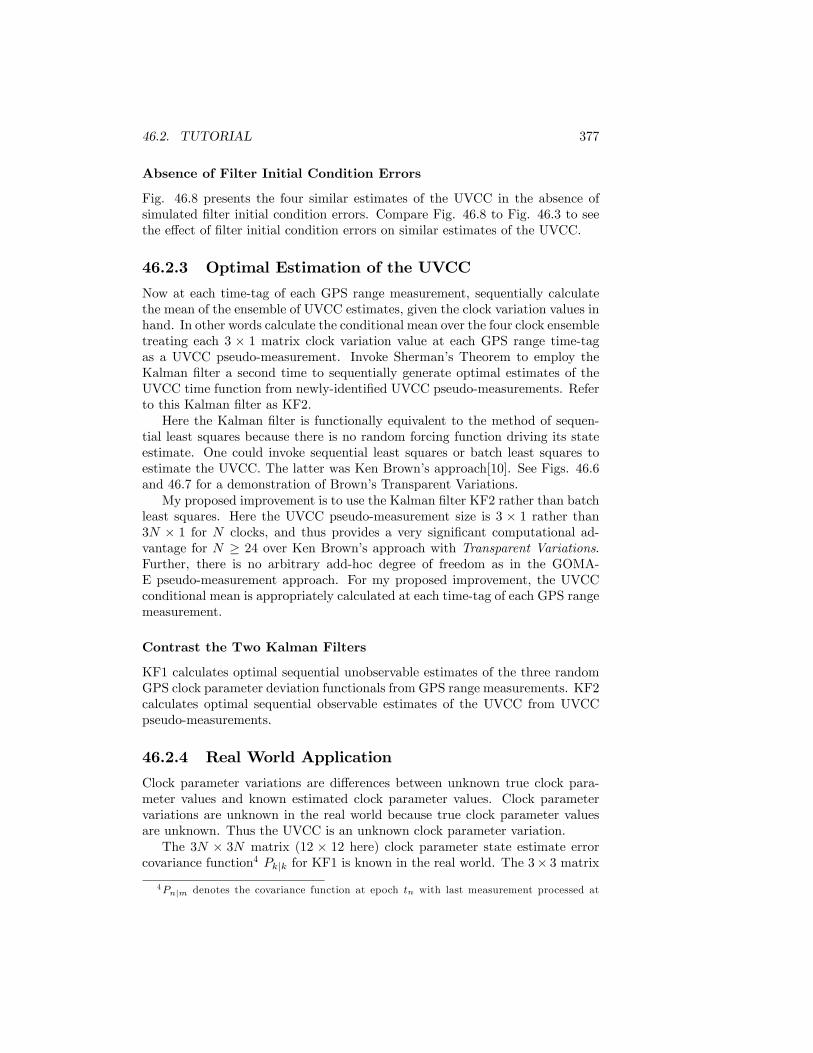
46.2. TUTORIAL 377
Absence of Filter Initial Condition Errors
Fig. 46.8 presents the four similar estimates of the UVCC in the absence ofsimulated �lter initial condition errors. Compare Fig. 46.8 to Fig. 46.3 to seethe e¤ect of �lter initial condition errors on similar estimates of the UVCC.
46.2.3 Optimal Estimation of the UVCC
Now at each time-tag of each GPS range measurement, sequentially calculatethe mean of the ensemble of UVCC estimates, given the clock variation values inhand. In other words calculate the conditional mean over the four clock ensembletreating each 3 � 1 matrix clock variation value at each GPS range time-tagas a UVCC pseudo-measurement. Invoke Sherman�s Theorem to employ theKalman �lter a second time to sequentially generate optimal estimates of theUVCC time function from newly-identi�ed UVCC pseudo-measurements. Referto this Kalman �lter as KF2.Here the Kalman �lter is functionally equivalent to the method of sequen-
tial least squares because there is no random forcing function driving its stateestimate. One could invoke sequential least squares or batch least squares toestimate the UVCC. The latter was Ken Brown�s approach[10]. See Figs. 46.6and 46.7 for a demonstration of Brown�s Transparent Variations.My proposed improvement is to use the Kalman �lter KF2 rather than batch
least squares. Here the UVCC pseudo-measurement size is 3 � 1 rather than3N � 1 for N clocks, and thus provides a very signi�cant computational ad-vantage for N � 24 over Ken Brown�s approach with Transparent Variations.Further, there is no arbitrary add-hoc degree of freedom as in the GOMA-E pseudo-measurement approach. For my proposed improvement, the UVCCconditional mean is appropriately calculated at each time-tag of each GPS rangemeasurement.
Contrast the Two Kalman Filters
KF1 calculates optimal sequential unobservable estimates of the three randomGPS clock parameter deviation functionals from GPS range measurements. KF2calculates optimal sequential observable estimates of the UVCC from UVCCpseudo-measurements.
46.2.4 Real World Application
Clock parameter variations are di¤erences between unknown true clock para-meter values and known estimated clock parameter values. Clock parametervariations are unknown in the real world because true clock parameter valuesare unknown. Thus the UVCC is an unknown clock parameter variation.The 3N � 3N matrix (12 � 12 here) clock parameter state estimate error
covariance function4 Pkjk for KF1 is known in the real world. The 3� 3 matrix4Pnjm denotes the covariance function at epoch tn with last measurement processed at

378 CHAPTER 46. GPS COMPOSITE CLOCK
pseudo-measurement residual covariance function, denoted here by CUV CCkjk , foreach KF2 UVCC pseudo-measurement is given by a 3�3 sub-matrix from Pkjk.This is all that is required to calculate the 3� 3 state estimate error covariancePUV CCkjk for the UVCC estimate. Thus PUV CCkjk is also known in the real world.
The evaluation of PUV CCkjk statistically quanti�es the di¤erence between eachKF1 estimate of UVCC and the unknown UVCC.Unbounded eigenvalues of Pkjk would eventually destroy KF1. Simulated
UVCC pseudo-measurements, observable to the KF1 state, could be processedwith GPS range measurements by KF1 so as to produce an appropriatelybounded covariance matrix ~Pkjk function for use in KF1. But it is su¢ cientto perform the measurement update on the KF1 state estimate error covariancePkjk using the pseudo-measurement residual covariance function CUV CCkjk , with-out actually simulating a UVCC measurement. Recursively applied, this wouldgenerate a bounded ~Pkjk for real world application.
Figure 46.1: Sim Phase Dev (units: 1� 10�7s) vs Time (0 - 8) d
time tm.

46.2. TUTORIAL 379
Figure 46.2: Sim & Est Phase Dev (units: 1� 10�7s) vs Time (0 - 8) d
Figure 46.3: 4 Similar Phase Var (units: 1� 10�7s) vs Time (0 - 8) d
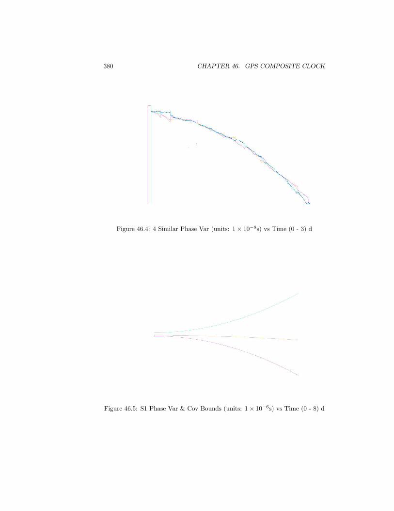
380 CHAPTER 46. GPS COMPOSITE CLOCK
Figure 46.4: 4 Similar Phase Var (units: 1� 10�8s) vs Time (0 - 3) d
Figure 46.5: S1 Phase Var & Cov Bounds (units: 1� 10�6s) vs Time (0 - 8) d

46.2. TUTORIAL 381
Figure 46.6: S1 Phase Var Reduced Cov (units: 1� 10�7s) vs Time (0 - 8) d
Figure 46.7: S1 Phase Var Reduced Cov (units: 1� 10�9s) vs Time (0 - 8) d

382 CHAPTER 46. GPS COMPOSITE CLOCK
Figure 46.8: 4 Similar Phase Var no IC (units: 1� 10�8s) vs Time (0 - 8) d

Part XIII
Appendices
383


A. The Least SquaresQuadratic
Given:
~J (�X0) = (�y �A�X0)TW (�y �A�X0)
one can derive:
@ ~J
@�X0= 2
�ATWA �X0 �ATW�y
�by di¤erentiating ~J (�X0) as though its elements were scalars but inserting thematrix transpose operator to obtain consistent matrix dimensionality. Note �rstthat:
@�y
@�XT0
= 0m�n
and:
@�X0
@�XT0
= In�n:
Then:
@ ~J
@�X0=
�@�y
@�XT0
�A @�X0
@�XT0
�TW (�y �A�X0)+
�(�y �A�X0)
TW
�@�y
@�XT0
�A @�X0
@�XT0
��T= �ATW�y +ATWA�X0 +
���yTWA+�XT
0 ATWA
�T= 2
�ATWA �X0 �ATW�y
�:
385

386 A. THE LEAST SQUARES QUADRATIC

B. Sequential Least Squares
The sequential least squares algorithm derives from the batch least squaresalgorithm, and is essentially equivalent to it given the least squares hypothesis.We are given an a priori state estimate n�1matrix X0j0 and mmeasurements
yj , where j 2 f1; 2; : : : ;mg. The iterative least squares normal equation is givenby Eq. 35.9: �
ATWA��X0jm = ATW�y (1)
where matrix A is an m�n (m > n) matrix, W is an m x m diagonal matrix ofmeasurement weights, �X0jm is an n � 1 state correction estimate at time t0,and �y is an m � 1 matrix of measurement residuals. The subscript notation0jm denotes epoch at time t0, and the inclusion of measurements through timetm.Eq. 1 can also be written:0@ mX
j=1
ATj WjAj
1A�X0jm =
0@ mXj=1
ATj Wj�yj
1A (2)
To see this, insert:
A =
26664A1A2...Am
37775
W =
26664W1 0
W2
. . .0 Wm
37775
�y =
26664�y1�y2...�ym
37775387

388 B. SEQUENTIAL LEAST SQUARES
into Eq. 1. Aj is 1 x n, Wj is 1 x 1, and:
�yj = yj � y�Xjj0
�(3)
is 1 x 1. yj is a measurement value, and the measurement representation
y�Xjj0
�is a nonlinear function of Xjj0. Measurement weight Wj is the recip-
rocal of white noise measurement error variance �2y;j :
�2y;j = 1=Wj : (4)
If the n� n matrix ATWA is non-singular (has no zero eigenvalues), then it isinverted to produce the state correction:
�X0jm =�ATWA
��1 �ATW�y
�(5)
The correction �X0jm is added to the a priori state estimate X0j0 at time t0,and Eq. 5 is iterated recursively until the sum of squares of weighted measure-ment residuals �yTW �y (weighted RMS squared) is less than some preassignedpositive small number, or until the iterative relative weighted RMS magnitudeon measurement residuals is less than some preassigned positive number. Itis important to note that the least squares algorithm is derived by minimizing�yTW�y.Matrix Aj is constructed from the product:where yj is the measurement representation for time tj , and the linear state
error transition matrix �j;0 moves state information from epoch at time t0 totime of measurement tj .It is well known by users of batch least squares orbit determination that
the best accuracy prediction performance is obtained empirically by �nding abatch time interval which is long enough to capture su¢ cient measurement in-formation, and is short enough to avoid the e¤ects of random force modelingerrors. Suppose here that m measurements requires an excessive batch measure-ment time interval, and that p < m measurements does satisfy the time intervalrequirement.Partition the batch of m measurements into two batches of sizes p and q: m
= p + q. Then tq = tm and equation 2 can be written:
0@ pXj=1
ATj WjAj +
p+qXj=p+1
ATj WjAj
1A�X0jq =
0@ pXj=1
ATj Wj�yj +
p+qXj=p+1
ATj Wj�yj
1A :
(6)Now suppose in real time that the last measurement we have received is at timetp. We do not yet have the measurement at time tp+1. The least squares normalequation can be written:0@ pX
j=1
ATj WjAj
1A�X0jp =
0@ pXj=1
ATj Wj�yj
1A ; (7)

389
similar to Eq. 2. The state correction estimate can then be calculated:
�X0jp =
0@ pXj=1
ATj WjAj
1A�10@ pXj=1
ATj Wj�yj
1A (8)
together with the least squares state error covariance matrix:
P0jp =
0@ pXj=1
ATj WjAj
1A�1
(9)
if the information matrix�Pp
j=1ATj WjAj
�is non-singular. Iterative di¤erential
corrections are performed as de�ned above. Now insert Eq. 9 into Eq. 6:
0@P�10jp + p+qXj=p+1
ATj WjAj
1A�X0jq =
0@ pXj=1
ATj Wj�yj +
p+qXj=p+1
ATj Wj�yj
1A :
(10)Suppose we have just received the second batch of q measurements. How shallwe use Eq. 10? Note that the n � 1 matrix
Ppj=1A
Tj Wj�yj is presumably
negligible due to minimizing �yTW�y over the �rst batch of p measurements.Then Eq. 10 can be written:0@P�10jp + p+qX
j=p+1
ATj WjAj
1A�X0jq =
0@ p+qXj=p+1
ATj Wj�yj
1A (11)
and the correction:
�X0jq =
0@P�10jp + p+qXj=p+1
ATj WjAj
1A�10@ p+qXj=p+1
ATj Wj�yj
1A (12)
can be calculated together with the least squares covariance matrix:
P0jq =
0@P�10jp + p+qXj=p+1
ATj WjAj
1A�1
(13)
if the least squares information matrix�P�10jp +
Pp+qj=p+1A
Tj WjAj
�is non-singular.
Given the least squares hypothesis, we note that �X0jq is essentially the samecorrection obtained in Eq. 5, but here we have obtained it sequentially in twomeasurement batches rather then one.Important: As Jim Woodburn emphatically notes, �X0jq is not the same
correction obtained in Eq. 5 when processing real data. This is due to existence

390 B. SEQUENTIAL LEAST SQUARES
of force modeling errors and the nonlinearty produced by iterative least squarescorrections.Recall from above we have assumed that the simultaneous processing of m
measurements requires an excessive batch measurement time interval [t1; tm];i.e., random force modeling errors are hurting us. Then Eq. 13 needs to bemodi�ed to decrease the in�uence of the a priori information matrix P�10jp =�Pp
j=1ATj WjAj
�on the state error correction estimate �X0jq of Eq. 12.
This is equivalent to increasing variances of the a priori covariance matrix
P0jp =�Pp
j=1ATj WjAj
��1. When this is performed the a priori information
matrix P�10jp is said to be deweighted and the batch least squares algorithm istransformed into a batch �lter.
C. Ad-Hoc Batch Filter
We have derived the batch least squares algorithm and the sequential leastsquares algorithm above. The batch �lter algorithm is derived below, ad hoc,from the sequential least squares algorithm.Swerling [103] derived a version of the batch �lter from the maximum like-
lihood quadratic form in 1958. This unitless quadratic form J has two terms:J = �yTW�y + �XT
0 P�10 �X0. The �rst term is the least squares quadratic
form and the second term is a quadratic form on the di¤erence �X0 between theprevious state estimate and the new state estimate, both at �xed epoch t0, andweighted by an a priori positive de�nite state error covariance matrix P0. Themaximum likelihood algorithm, derived by minimization of J , can be viewed asminimizing the sum of squares of measurement residuals while simultaneouslyconstraining the new state estimate to the previous state estimate. The batch�lter is an intermediate method that has characteristics of both a least squaresalgorithm and a �lter. From a user perspective, the maximum liklihood algo-rithm is distinguished from least squares in that it enables the speci�cation ofan a priori state error covariance matrix to constrain the new state estimate tothe previous state estimate. The user typically speci�es a positive diagonal apriori covariance matrix, with large values to free the new state estimate fromthe a priori state estimate, and/or small values to bind the new state estimate tothe a priori state estimate. Swerling did not discover Schur�s matrix identities(inversion lemma, see Meditch [76]), and was thereby blocked from removingthe debilitating n � n matrix inverse with state size n, associated with leastsquares and the batch �lter. The inversion lemma is required to convert fromsimultaneous measurement batch processing to sequential processing withoutthe n � n matrix inverse. Sequential processing is a necessary condition foroptimal estimation. It was left to Kalman to discover Sherman�s theorem andthereby introduce a stochastic performance functional for optimal estimation.Recall Eq. 34.11, and de�ne:
�j;i =@Xj
@Xi(14)
for any times ti and tj . Insert Aj = Hj�j;0 and Wj = R�1j (recall Eqs. 34.13and ??) into Eqs. 9, 12 and 13 to get:
391

392 C. AD-HOC BATCH FILTER
P0jp =
0@ pXj=1
(Hj�j;0)TR�1j (Hj�j;0)
1A�1
(15)
�X0jq = P0jq
0@ p+qXj=p+1
(Hj�j;0)TR�1j �yj
1A (16)
P0jq =
0@P�10jp + p+qXj=p+1
(Hj�j;0)TR�1j (Hj�j;0)
1A�1
: (17)
Our least squares epoch was arbitrarily selected to be time t0. We could justas easily have selected time tq for epoch. In this case the above three equationsbecome:
Pqjp =
0@ pXj=1
(Hj�j;q)TR�1j (Hj�j;q)
1A�1
(18)
�Xqjq = Pqjq
0@ p+qXj=p+1
(Hj�j;q)TR�1j �yj
1A (19)
and:
Pqjq =
0@P�1qjp + p+qXj=p+1
(Hj�j;q)TR�1j (Hj�j;q)
1A�1
: (20)
Premultiply Eq 18 by �p;q, post multiply it by �Tp;q, and use the transitiveproperty �r;p = �r;q�q;p with r = p and �p;p = I to get �p;q = ��1q;p and:
Ppjp =
0@ pXj=1
(Hj�j;p)TR�1j (Hj�j;p)
1A�1
(21)
to see that Eq. 18 can be written:
Pqjp = �q;pPpjp�Tq;p: (22)
Eqs. 19, 20, 22, and 21 de�ne the exact same sequential least squares algorithmderived in Appendix B, but with di¤erent epoch placement. With these changesin epoch placement, the last paragraph of Appendix B reads: Then Eq. 22 needsto be modi�ed to decrease the in�uence of the a priori information matrix P�1pjpon the state error correction estimate �Xqjq of Eq. 19. This is equivalent toincreasing variances of the a priori covariance matrix Ppjp, embedded in Eq. 22.

393
Thus the conversion of this sequential least squares algorithm to a batch �lteris achieved by replacing, ad hoc, covariance matrix Pqjp = �q;pPpjp�Tq;p with:
Pqjp = �q;pPpjp�Tq;p +Qq;p: (23)
For each measurement batch recursion, the batch �lter algorithm executionconsists of a time update and a measurement update. Assume that we havejust �nished processing the measurement batch at time tp, and that the nextmeasurement batch time is tq > tp. Given the state estimate Xpjp at time tp,it is numerically integrated to time tq to obtain Xqjp, the state estimate timeupdate. Then the state error covariance time update is de�ned by Eq. 23. Thenthe state error covariance measurement update is de�ned by Eq 20. Then thestate estimate measurement update is de�ned by Eq. 19 and:
Xqjq = Xqjp +�Xqjq: (24)
Given the next measurement batch time at tr > tq, then repeat the aboveprocedure with p! q and q ! r.The sums
Pp+qj=p+1 (Hj�j;q)
TR�1j �yj and
Pp+qj=p+1 (Hj�j;q)
TR�1j (Hj�j;q)
of Eqs. 19 and 20 are processed simultaneously, they de�ne the measurementbatch in �batch �lter�. Simultaneous batch processing is obviously faster thanindividual measurement processing.It must be noted that any optimal physically connected sequential �lter
processes each measurement separately, folding in measurement information�yj and force modeling error covariance Qj sequentially as they occur. Theoptimal real time �lter does not process any batch of measurements simulta-neously, for this destroys both optimal estimate accuracy and the autonomousmeasurement residual editor.Finally, given a rigorous derivation of an optimal physically connected se-
quential �lter from the fundamental theorem of estimation theory [76], one can�derive� the batch �lter from it with a degrading ad-hoc replacement: Ar-bitrarily replace any sequence of measurement/deweighting calculations witha simultaneous batch calculation (thereby ignoring all random force modelingerrors between measurement times) and retain deweighting at times betweenbatches.

394 C. AD-HOC BATCH FILTER

D. Kalman�s ModelEquation
Calculus provides the de�nition:
dX
dt= lim
�t!0
X (t+�t)�X (t)�t
= lim�t!0
�X
�t(25)
Thus the deterministic linear di¤erential equation:
dX
dt= A (t)X +B (t)! (26)
can be written:
lim�t!0
�X
�t= A (t)X +B (t)! (27)
Undo the calculus (remove the limit) to write:
�X = A (t)X�t+B (t)!�t (28)
Transform this deterministic equation to a stochastic equation with the whitenoise assignment:
! =��
�t(29)
according to Eq. 12.95, where � is Brownian motion. Thus:
�X = A (t)X�t+B (t)�� (30)
provides a well-de�ned linear ordinary stochastic di¤erential equation wherevariations �X in the state are driven by independent increments (white noise)�� of Brownian motion. See Bucy [9] page 24 Eq. 2.5 for comparison.
.0.5 Measurements at tj = tk+1; tk+2; : : :
In the section Measurement at tj = tk+1 above, replace tk+1 with tk+2 for themeasurement yj = yk+2 at time tj = tk+2. When tj = tk+h, replace tk+1 withtk+h for the measurement yj = yk+h at time tj = tk+h.
395

396 D. KALMAN�S MODEL EQUATION

Bibliography
[1] Allan, D.W., Time and Frequency Characterization, Estimation, and Pre-diction of Precision Clocks and Oscillators, NIST Technical Note 1337,1990
[2] Antreasian, Peter Garo, Precision Radiation Force Modeling for theTOPEX/POSEIDON Mission, Phd Thesis, University of Colorado, 1992
[3] Baker, Robert M.L., Astrodynamics: Applications and Advanced Topics,Academic Press, New York, 1967
[4] Bancroft, Stephen, "An Algebraic Solution of the GPS Equations." IEEETransactions on Aerospace and Electronic Systems, Vol. AES-21, No. 7,January, 1985.
[5] Bar-Sever, Y., Kuang, D., "New Empirically Derived Solar RadiationPressure Model for Global Positioning System Satellites", IPN ProgressReport 42-159, November 15, 2004.
[6] Bar-Sever, Y., Kuang, D., "New Empirically Derived Solar RadiationPressure Model for Global Positioning System Satellites During EclipseSeasons", IPN Progress Report 42-160, February 15, 2005.
[7] Adi Ben-Israel, Thomas N. E. Greville, Generalized Inverses: Theory andApplication, Wiley, New York, 1974
[8] Gerald J Bierman, Factorization Methods for Discrete Sequential Estima-tion, Academic Press, New York, 1977
[9] Bucy, Richard S., Joseph, Peter D., Filtering for Stochastic Processes withApplications to Guidance, Interscience Publishers, John Wiley & Sons,New York, 1968
[10] Brown, Kenneth R., The Theory of the GPS Composite Clock, Proc. Inst.Navig.�Global Posit. Syst., 1991, pp. 223-241
[11] Budden, K., G., The Propagation of Radio Waves, Cambridge UniversityPress,England, 1972
397

398 BIBLIOGRAPHY
[12] The Committee for the COSPAR International Reference Atmosphere(CIRA) of COSPAR Working Group 4, Committee On Space Research(COSPAR), CIRA 1972, Akademie-Verlag, Berlin, 1972
[13] Collins, J. Paul, An Overview of GPS Inter-Frequency Carrier Phase Com-binations, UNB/GSD, October 1999 (WEB)
[14] R. K. Crane, M. L. Meeks, "Refraction E¤ects in the Neutral At-mosphere", Methods of Experimental Physics: Astrophysics 12B, Acad-emic Press, 1976
[15] Davenport, Wilbur B., Root, William L., An Introduction to RandomSignals and Noise, McGraw-Hill, New York, 1958
[16] J. L. Davis, T. A. Herring, I. I. Shapiro, A. E. E. Rogers, G. Elgered,Geodesy by Radio Interferometry: E¤ects of Atmospheric Modeling Errorson Estimates of Baseline Length, Radio Science, vol. 20, 1985.
[17] Daniel N. Lapedes, McGraw-Hill Dictionary of Physics and Mathematics,McGraw-Hill Book Company, New York, 1978
[18] Doob, J. L., Stochastic Processes, John Wiley & Sons, New York, 1953.
[19] Paul Dyer and Stephen McReynolds, Extension of Square Root Filteringto Include Process Noise, J. Ops. Theory and Appl. 3, No. 6, 444-459,1969
[20] Feller, W., An Introduction to Probability Theory and its Applications,Vol. 1, John Wiley & Sons, New York, 1950.
[21] Feller, W., An Introduction to Probability Theory and its Applications,Vol. 2, John Wiley & Sons, New York, 1970, pp. 262-3.
[22] Fliegel, H.F., Gallini, T.E., Swift, E.R., "Global Positioning System Ra-diation Force Model for Geodetic Applications", Journal of GeophysicalResearch, Volume 97, No. B1, January 1992.
[23] Fliegel, H.F., Gallini, T.E., "Solar Force Modeling of Block IIR GlobalPositioning System Satellites", Journal of Spacecraft and Rockets, Volume33, No. 6, November-December 1996.
[24] Foster, J., Richards, F. B., The Gibbs Phenomenon for Piecewise-LinearApproximations, The American Mathematical Monthly, Vol. 98, No. 1.Jan., 1991, pp. 47-49
[25] Gauss, K. F., Theoria Motus Corporum Coelestium (Theory of the Motionof the Heavenly Bodies Moving about the Sun in Conic Sections), Little,Brown, and Co., 1857, republished by Dover, 1963
[26] J. Willard Gibbs, Vector Analysis, Dover Edition, 1960, from CharlesScribner�s & Sons, 1909

BIBLIOGRAPHY 399
[27] Paul Glasserman, Monte Carlo Methods in Financial Engineering,Springer, 2004
[28] Gene H. Golub, Charles F. Van Loan, Matrix Computations, Johns Hop-kins Press, 1989
[29] Gooding, R. H., A New Procedure for Orbit Determination Based on ThreeLines of Sight (Angles Only), Technical Report 93004, Defense ResearchAgency (GU14 6TD UK), Farnborough, Hampshire, April 1993
[30] Gooding, R. H., On the Solution of Lambert�s Orbital Boundary-ValueProblem, Technical Report 88027, Royal Aerospace Establishment, Pro-curement Executive, Minister of Defence, Farnborough, Hants, 1988
[31] GEONS Time Bias Propagation, GSFC, FDSS-14-0006, pages 4-36through 4-39
[32] Herrick, Samuel, Astrodynamics, Vol 1, Van Nostrand, London, 1971
[33] Herrick, Samuel, Astrodynamics, Vol 2, Van Nostrand, London, 1972
[34] T. A. Herring, Modeling Atmospheric Delays in the Analysis of SpaceGeodetic Data, Proceedings of the Symposium on Refraction of Transat-mospheric Signals in Geodesy, Netherlands, Delft, No. 36, New Series, pp157-164, 1992.
[35] Ho, Y.C., The Method of Least Squares and Optimal Filtering Theory,Rand Corporation, Oct 1962
[36] D. B. Holdridge, An Alternate Expression for Light Time Using GeneralRelativity, JPL Space Program Summary 37-48, III, pp. 2-4. This referenceis given in McCarthy[70].
[37] A. S. Householder, Unitary Triangularization of a Nonsymmetric Matrix,J. Ass. Comp. Mach. 5, 205-243, 1958
[38] Hughes, Peter C., Spacecraft Attitude Dynamics, JohnWiley & Sons, 1988.pp. 522-34.
[39] Hujsak, R.S., Solar Pressure, Proceedings of the Arti�cial Satellite TheoryWorkshop, Edited by P. Kenneth Seidelmann and Bernard Kaufman, U.S.Naval Observatory, Washington DC, Nov 8,9, 1993
[40] GPS NAVSTAR JPO, ICD-GPS-200, REV. C, 10 October 1993, NAVS-TAR GPS Space Segment/Navigation User Interface, IRN-200C-004, 12April 2000
[41] GPS NAVSTAR JPO, ICD-GPS-208, 5 June 1987, Auxilary User Inter-faces
400 BIBLIOGRAPHY
[42] I. M. Ifadis, Space to Earth Geodetic Observations: Approaching the At-mospheric E¤ect, Aristotle University, (1999 - latest reference)
[43] I. M. Ifadis, A New Approach to Mapping the Atmospheric E¤ect for GPSObservations, Aristotle University, Earth Planets Space, 52, 703-708, 2000
[44] I. Ifadis, The Atmospheric Delay of Radio Waves: Modelling the ElevationDependence on a Global Scale, Licentiate Thesis, Technical Report No.38L, Gothburg, Sweden, 1986
[45] I. Ifadis, Contribution to the Study of the Atmospheric Refraction, on Ra-dio Waves Used in Modern Geodetic Techniques in Long Distance Mea-surements, Thesis Report, vol. IA�.6, School of Engineering, Faculty ofCivil Engineering, Thessalonika, 1987.
[46] Eugene Jahnke, Fritz Emde, Tables of Functions with Formulae andCurves, Dover, New York, 1945
[47] Johnson, N.J., S. Kotz, N. Balakrishnan (1994), Continuous UnivariateDistributions, Vol. 1, 2nd ed., John Wiley & Sons, New York. p. 91.
[48] Kalman, R. E., New Methods in Wiener Filtering Theory, Proceedings ofthe First Symposium on Engineering Applications of Random FunctionTheory and Probability, edited by J. L. Bogdano¤ and F. Kozin, JohnWiley & Sons, New York, 1963.
[49] Kaplan, Elliott D. (editor), Ward, Phillip (Chapter 5), UnderstandingGPS, Artech House, Boston, 1996E.
[50] Kaula, William M., Theory of Satellite Geodesy, Blaisdell Pub., Mass.,1966
[51] Kaula, William M., Statistical and Harmonic Analysis of Gravity, Journalof Geophysical Research, Vol. 64, Dec. 1959, pp. 2411, 2412, 2418.
[52] King-Hele, Desmond, Theory of Satellite Orbits in an Atmosphere, But-terworths, London, 1964
[53] Klobuchar, J. A., The Handbook of Geophysics and the Space Environ-ment, Air Force Geophysics Laboratory, 1985
[54] Konopliv, A.S., S.W. Asmar, E. Carranza, W.L. Sjogren, and D.N. Yuan(2001), "Recent Gravity Models as a Result of the Lunar Prospector Mis-sion", Icarus, Volume 150, Issue 1, March 2001, Pages 1-18.
[55] Paul E. Koskela (L. G. Walters, C. G. Hilton, J. L. Arsenault, R. G.Schinnerer, Chela Varrentzo¤, K. C. Ford), Astrodynamic Analysis forthe Advanced Orbit/Ephemeris Subsystem, Aeronutronic Pub. No. U-4180,DDI Subcontract No. 66-1, AF 04(695)-976, Philco-Ford AeronutronicDiv, 1 Sep., 1967

BIBLIOGRAPHY 401
[56] Kursinski et. al., The GPS Radio Occultation Technique, TAO, Vol. 11,No. 1, 53-114, March, 2000.
[57] Lancaster, E. R., Blanchard, R. C., A Uni�ed Form of Lambert�s Theorem,NASA TN D-5368, Sept. 1969
[58] Richard B. Langley, Wendy Wells, Virgilio de Brito Mendes, TroposphericPropagation Delay: a Bibliography, Geodetic Research Library, De-partment of Geodesy and Geomatics Engineering, University of NewBrunswick, 2nd Edition, 22 April 1995
[59] Harry Lass, Vector and Tensor Analysis, McGraw-Hill, New York, 1950
[60] Larson, Kristine, Levine, Judah, Time Transfer Using the Phase of theGPS Carrier, IEEE Transactions on Ultrasonics, Ferroelectrics, and Fre-quency Control, Vol. 46, No. 4, July 1999
[61] Larson, Kristine, Levine, Judah, Carrier Phase Time Transfer, IEEETransactions on Ultrasonics, Ferroelectrics, and Frequency Control, Vol.47, No. 2, March 2000
[62] Link, F., Lunar Eclipses, Physics and Astronomy of the Moon, edited byKopal, Academic Press, New York, 1962
[63] Larson, Kristine, Levine, Judah, Nelson, Lisa M., Parker, Thomas E.,Assessment of GPS Carrier-Phase for Time-Transfer Applications, IEEETransactions on Ultrasonics, Ferroelectrics, and Frequency Control, Vol.46, No. 4, July 1999
[64] Larson, Kristine, Private Communication (e-mail), 9 July 2007
[65] Charles L. Lawson, Richard J. Hanson, Solving Least Squares Problems,Prentice-Hall, 1974
[66] Robert G. Lorenz (Assignee: Ashtech Telesis, Inc.), GPS CommercialReceiver Patent Number 5,134,407, U. S. Patent Documents, 28 July 1992.
[67] Robert G. Lorenz (Assignee: Ashtech Telesis, Inc.), GPS CommercialReceiver Patent Number 5,293,170, U. S. Patent Documents, 8 March1994.
[68] J. W. Marini, Correction of Satellite Tracking Data for an arbitrary At-mospheric Pro�le, Radio Science, vol. 7, pp223-231, 1972.
[69] McCarthy, D., IERS Standards, IERS Technical Note 13, 1992
[70] Dennis D. McCarthy, IERS Technical Note 21, US Naval Observatory,July 1996. See Eq. 17 therein.
[71] McCarthy, Dennis D., IERS TECHNICAL NOTE 32, US Naval Observa-tory, Nov., 2003

402 BIBLIOGRAPHY
[72] Stephen McReynolds, Private Communications, 1980 to 1998.
[73] Stephen McReynolds, Editing Data Using Sequential Smoothing Tech-niques for Discrete Systems, AIAA/AAS Astrodynamics Conference, Au-gust 20-22, 1984, Seattle, WA.
[74] Stephen McReynolds, Filter-Smoother Consistency Test, Intero¢ ceMemo, Martin Marietta, 21 Feb., 1995
[75] McReynolds, S.R. "Multipoint Smoothing Algorithm Systems", Journalof Guidance, Control, and Dynamics, Vol. 12, Number 6, Nov-Dec 1989,pages 920-924.
[76] Meditch, J. S., Stochastic Optimal Linear Estimation and Control,McGraw-Hill, New York, 1969.
[77] Meditch, J. S., Orthogonal Projection and Discrete Optimal LinearSmoothing, SIAM J. Control, vol. 5, p. 74, 1967
[78] Meditch, J. S., A Survey of Data Smoothing for Linear and NonlinearDynamic Systems, Automatica, Vol. 9, pp. 151-162, 1973
[79] Meditch, J. S., Personal Communications, The Aerospace Corporation,1974.
[80] Meditch, J. S., Personal Communications, 1974.
[81] Thomas K. Meehan, Jess Brooks, Lawrence E. Young (Assignee: Califor-nia Institute of Technology), GPS Receiver Patent Number 6,061,390, U.S. Patent Documents, 9 May 2000.
[82] V. B. Mendes, R. B. Langley, A Comprehensive Analysis of Mapping Func-tions Used in Modeling Tropospheric Propagation Delay in Space GeodeticData, Paper at KIS94, Ban¤, Aug 30 �Sep 2, 1994
[83] C. Moller, The Theory of Relativity, Oxford University Press, Delhi, 1952,Clarendon Press 1972
[84] Anderson, Brian D. O., Moore, John B., Optimal Filtering, Prentice-Hall,New Jersy, 1979.
[85] Oliver Montenbruck, Remco Kroes, In-Flight Performance Analysis of theCHAMP Blackjack GPS Receiver, Rev. 1, 31 March 2003.
[86] Moyer, Theodore D., �Formulation for Observed and Computed Valuesof Deep Space Network Data Types for Navigation�, Monograph 2, DeepSpace Communications and Navigation Series.
[87] A. E. Niell, Improved Global Atmospheric Mapping Functions for VLBIand GPS, URSI/IAU Symposium on VLBI Technology � Progress andFuture Observational Possibilities, Kyoto, Japan, 6-10 Sepyrmber 1993.

BIBLIOGRAPHY 403
[88] A. E. Niell, Global Mapping Functions for the Atmospheric Delay at RadioWavelengths, J. Geophys. Res., 101(B2), 3227-3276, 1996
[89] A. Niell, The IMF Mapping Functions, 15 Aug 2002. This paper wasdownloaded from the WEB.
[90] O�Toole, James W., "Mathematical Description of the OMNIS SatelliteOrbit Generation Program (OrbGen)", NSWCDD/TR-02/118, May 2004.
[91] J. S. Owens, Optical Refractive Index of Air: Dependence on Pressure,Temperature, and Composition, Applied Optics, vol. 6, No. 1, pp 51-59,1967.
[92] Papoulis, A., Probability, Random Variables, and Stochastic Processes,McGraw-Hill, New York, 1965.
[93] Parker, Thomas E., Private Communication (Geneva), 30 May 2007
[94] Pechenick, K. R., Solar Radiation Pressure on Satellites and Other RelatedE¤ects, The General Electric Company, 1983
[95] Pechenick, K. R., A Derivation of the Gravity Error Covariance FormulasIncluding the O¤-Diagonal Components, Applied Technology Associates(ATA), GSFC Contract No. NAS5-29417, September 1988
[96] Rauch, H. E., Solutions to the Linear Smoothing Problem, IEEETrans.Autom. Control, vol. AC-8, p. 371, 1963
[97] Rauch, H. E., Tung, F., Striebel, C. T., Maximum Likelihood Estimatesof Linear Dynamical Systems, AIAA J., vol 3, p. 1445, 1965
[98] Davenport, Wilbur B., Root, William L., An Introduction to the Theoryof Random Signals and Noise, McGraw-Hill, New York, 1958.
[99] Schmidt, Stanley F., Compensation for Modeling Errors in Orbit Deter-mination Problems (Interim Report), Report No. 67-16, Contract NAS5-11048, November 1967, Analytical Mechanics Associates, Inc., 57 OldCountry Rd, Westbury, NY, 11590
[100] Sherman, S., A Theorem on Convex Sets with Applications, Ann. Math.Stat., 26, 763-767, 1955.
[101] Sherman, S., Non-Mean-Square Error Criteria, IRE Transactions on In-formation Theory, Vol. IT-4, 1958.
[102] Digital Systems Section Code 531, Tracking and Acquisition Handbookfor the Spacecraft Tracking and Data Network, 450-TAH-STDN, October1994, Section 4.2.2.3 Data Reduction Algorithms, subsection c. ObservedRange-Rate.

404 BIBLIOGRAPHY
[103] Swerling, P. A Proposed Stagewise Di¤erential Correction Procedure forSatellite Tracking and Prediction, P-1292, Rand Corporation, 8 Jan 1958
[104] Zucca, Cristina; Tavella, Patricia, The Clock Model and Its Relationshipwith the Allan and Related Variances, IEEE Transactions on Ultrasonics,Ferroelectrics, and Frequency Control, Vol. 52, No. 2, Feb. 2005
[105] A. M. Smith, REFRACTION CORRECTION, �RC, TM-(L)-5048/492/01, System Development Corporation, 11 August, 1978
[106] Phung, P. B., Guedeney, V. S., Teles, J., Tracking and Data Relay SatelliteSystem (TRDSS) Range and Doppler Tracking System Observation Mea-surement and Modeling, X-572-80-26, NASA GSFC, Sept. 1980, Equation4-2 and its derivation.
[107] Thayer, G. D., An Improved Equation for the Radio Refractive Index ofAir, Radio Science, vol. 9, pp. 803-807, 1974.
[108] Thode, Henry C. Jr.Testing for Normality, CRC Press, 2002.
[109] U.S. Air Force by Boeing Navigation Systems, GPS Operational ControlSystem Mathematical Algorithms Document, Volume GOMA-E, 27 Sep.,2005. Distribution authorized to US DOD and its contractors only.
[110] O. A. Vasicek, An Equilibrium Characterization of the Term Structure,Journal of Financial Economics, 5:177-188
[111] Vokrouhlicky, D., Farinella, P., Mignard, F., Solar Radiation Pres-sure Perturbations for Earth Satellites, I: A Complete Theory IncludingPenumbra Transitions, Astronomy and Astrophysics, 17.3, 1993
[112] Benton, William (publisher), Webster�s Third New International Dictio-nary of the English Language Unabridged, Encyclopaedia Britannica, Inc,Chicago, 1966
[113] Mark L. Wencek, The Hydrosphere, www.cmmp.ucl.ac.uk~jhh/2B27/water.rtf
[114] Wiberg, D. M., Theory and Problems of State Space and Linear Systems,Schaum�s Outline Series, McGraw-Hill, New York, 1971.
[115] J. H. Wilkinson, The Algebraic Eigenvalue Problem, Clarendon Press, Ox-ford, 1965
[116] Jacob Williams, E. Glenn Lightsey, SungPil Yoon, Robert E. Shutz, Test-ing of the ICESat Blackjack GPS Receiver Engineering Model, Center forSpace Research, The University of Texas at Austin, downloaded fromWEB, no date given.
[117] Wright, J. R., Sequential Orbit Determination with Auto-Correlated Grav-ity Modeling Errors, AIAA, Journal of Guidance and Control, Vol 4, No.2, May-June 1981, page 304.

BIBLIOGRAPHY 405
[118] Wright, J. R., Orbit Determination Solution to the Non-Markov GravityError Problem, AAS/AIAA Paper AAS 94-176, AAS/AIAA Space�ightMechanics Meeting, Cocoa Beach, FLA, Feb., 1994
[119] Wright, James R., Optimal Orbit Determination, Paper AAS 02-192,AAS/AIAA Space Flight Mechanics Meeting, San Antonio, Texas, 27-30Jan., 2002
[120] Wright, James R., Real-Time Estimation of Local Atmospheric Density,Paper AAS 03-164, 13th AAS/AIAA Space Flight Mechanics Meeting,Ponce, Puerto Rico, 9-13 Feb., 2003
[121] Wright, James R., Woodburn, James, Simultaneous Real-Time Estimationof Atmospheric Density and Ballistic Coe¢ cient, Paper AAS 04-175, 14thAAS/AIAA Space Flight Mechanics Conference, Maui, Hawaii, 8-12 Feb.,2004
[122] Wright, James R., Tanygin, Sergei, Removal of Arbitrary Discontinu-ities in Atmospheric Density, Paper AAS 04-176, 14th AAS/AIAA SpaceFlight Mechanics Conference, Maui, Hawaii, 8-12 Feb., 2004
[123] Wright, James R., Sherman�s Theorem, The Malcolm D. Shuster Astro-nautics Symposium, The Journal of the Astronautical Sciences, Vol. 54,Nos. 3 and 4, July - December 2006, pp. 299 - 319
[124] Wright, James R, Woodburn, James, Truong, Son, Chuba, William, OrbitGravity Error Covariance, Paper AAS 08-157, 18th AAS/AIAA SpaceFlight Mechanics Meeting, Galveston, Texas, January 2008
[125] Wright, James R, Woodburn, James, Truong, Son, Chuba, William, Sam-ple Orbit Covariance Function and Filter-Smoother Consistency Tests,Paper AAS 08-159, 18th AAS/AIAA Space Flight Mechanics Meeting,Galveston, Texas, January 2008
[126] Wright, James R, Woodburn, James, Truong, Son, Chuba, William, OrbitCovariance Inner Integrals with Polynomials, Paper AAS 08-161, 18th
AAS/AIAA Space Flight Mechanics Meeting, Galveston, Texas, January2008
[127] Wright, James R, GPS Composite Clock Analysis (two-state clocks), Hin-dawi Publishing Corporation, International Journal of Navigation and Ob-servation, Volume 2008, Article ID 261384
[128] Wright, James R, Composite Clocks with Three-State Models, Paper 33,Thirty-Ninth Annual Precise Time and Time Interval (PTTI) Systemsand Applications Meeting, Hyatt Regency, Long Beach, CA, November2007

406 BIBLIOGRAPHY
[129] Wright, James R, Woodburn, James, Nonlinear Variable Lag Smoother,F. Landis Markley Astronautics Symposium, American Astronautical So-ciety, Cambridge, Maryland, July 2, 2008
[130] Wu, S. C., et. al, Global Positioning System (GPS) Precision Orbit De-termination (POD) Software Design, TOPEX/Poseidon Project, JPL D-7275, March 9, 1990.
[131] Ming YANG and Kuo-Hwa CHEN, "Performance Assessment of a Nonit-erative Algorithm for GPS Absolute Positioning", Proc. Natl. Sci. Counc.ROC(A) Vol. 25, No. 2, 2001, pp. 102-106.