October 2013MSc SAI - Parallel & Concurrent (J Paul Gibson) Parallel and Concurrent Programming...
208
October 2013 MSc SAI - Parallel & Concurrent (J Paul Gibson) rallel and Concurrent Programming Motivation (General): •Multicore Architectures •Systems that require High Performance Computing (HPC) services •Systems that provide HPC services •Science and Engineering moving towards simulation (requiring HPC) Motivation (Software Engineering): •Understanding the interaction between hardware and software is key to making architectural tradeoffs during design (for HPC) •It is also important to understand the need to balance potential gains in performance versus additional programming effort involved. 1
-
date post
19-Dec-2015 -
Category
Documents
-
view
241 -
download
2
Transcript of October 2013MSc SAI - Parallel & Concurrent (J Paul Gibson) Parallel and Concurrent Programming...

MSc SAI - Parallel & Concurrent (J Paul Gibson) 1October 2013
Parallel and Concurrent Programming
Motivation (General):
•Multicore Architectures
•Systems that require High Performance Computing (HPC) services
•Systems that provide HPC services
•Science and Engineering moving towards simulation (requiring HPC)
Motivation (Software Engineering):
•Understanding the interaction between hardware and software is key to making architectural tradeoffs during design (for HPC)
•It is also important to understand the need to balance potential gains in performance versus additional programming effort involved.
MSc SAI - Parallel & Concurrent (J Paul Gibson) 2October 2013
Multi-Core

MSc SAI - Parallel & Concurrent (J Paul Gibson) 3October 2013
Multi-Core

MSc SAI - Parallel & Concurrent (J Paul Gibson) 4October 2013
Multi-Core
MSc SAI - Parallel & Concurrent (J Paul Gibson) 5October 2013
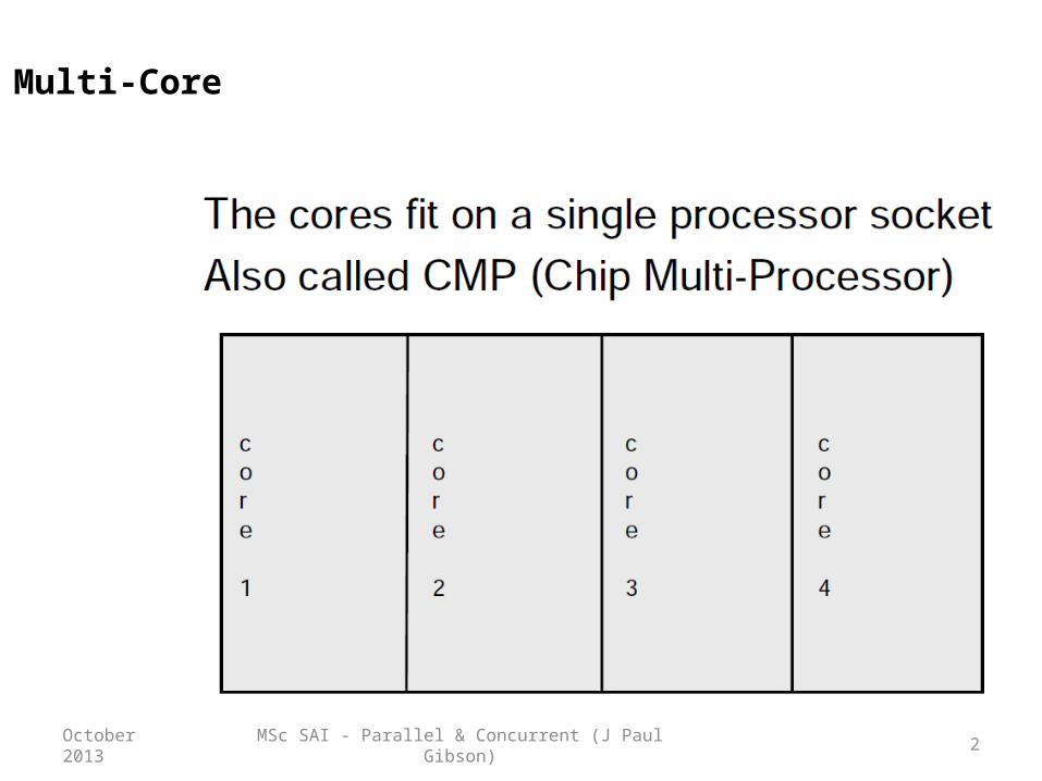
Multi-Core
Multi-core processors are MIMD:Different cores execute different threads(Multiple Instructions), operating on differentparts of memory (Multiple Data).
Multi-core is a shared memory multiprocessor:All cores share the same memory

MSc SAI - Parallel & Concurrent (J Paul Gibson) 6October 2013
Multi-Core
Interaction with the Operating System:
• OS perceives each core as a separate processor• OS scheduler maps threads/processes to different cores• Most major OS support multi-core today: Windows, Linux, Mac OS X, …
Why multi-core ?• Difficult to make single-core clock frequencies even higher• Deeply pipelined circuits:
– heat problems– speed of light problems– difficult design and verification– large design teams necessary– server farms need expensive air-conditioning
• Many new applications are multithreaded• General trend in computer architecture (shift towards more parallelism)
MSc SAI - Parallel & Concurrent (J Paul Gibson) 7October 2013
Multi-Core
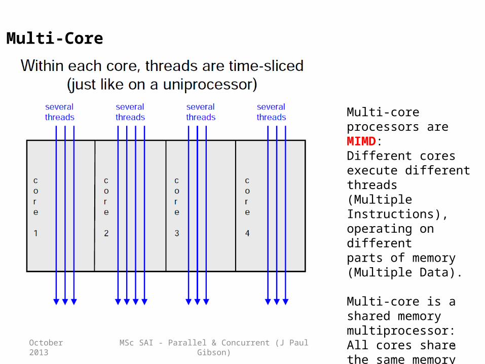
Instruction-level parallelism:
• Parallelism at the machine-instruction level• The processor can re-order, pipeline instructions, split them into microinstructions, do aggressive branch prediction, etc.• Instruction-level parallelism enabled rapid increases in processor speeds over the last 15 years
Thread-level parallelism (TLP):
• This is parallelism on a more coarser scale• Server can serve each client in a separate thread (Web server, database server)• A computer game can do AI, graphics, and physics in three separate threads• Single-core superscalar processors cannot fully exploit TLP• Multi-core architectures are the next step in processor evolution: explicitly exploiting TLP
MSc SAI - Parallel & Concurrent (J Paul Gibson) 8October 2013
Multi-Core
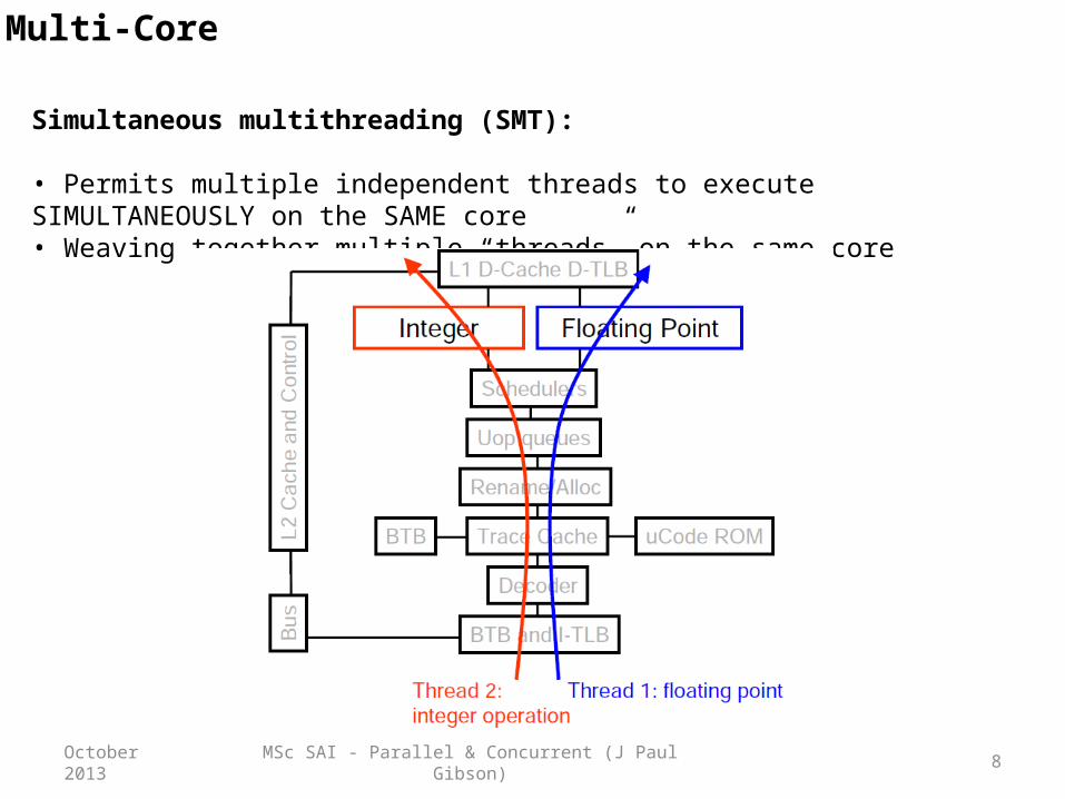
Simultaneous multithreading (SMT):
• Permits multiple independent threads to execute SIMULTANEOUSLY on the SAME core• Weaving together multiple “threads” on the same core
MSc SAI - Parallel & Concurrent (J Paul Gibson) 9October 2013
Multi-Core
Combining Multi-core and SMT
• Cores can be SMT-enabled (or not)
• The different combinations:– Single-core, non-SMT: standard uniprocessor– Single-core, with SMT– Multi-core, non-SMT– Multi-core, with SMT:
• The number of SMT threads:2, 4, or sometimes 8 simultaneous threads
• Intel calls them “hyper-threads”
MSc SAI - Parallel & Concurrent (J Paul Gibson) 10October 2013
Parallel and Concurrent Programming
There is a confusing use of terminology:
•Parallel – "The simultaneous use of more than one computer to solve a problem“
•Concurrent – "Concurrent computing is a form of computing in which programs are designed as collections of interacting computational processes that may be executed in parallel "
•Distributed – "A collection of (probably heterogeneous) automata whose distribution is transparent to the user so that the system appears as one local machine."
•Cluster – "Multiple servers providing the same service"
•Grid – “ A form of distributed computing whereby a “super virtual computer” is composed of many networked loosely coupled computers acting together to perform very large tasks. "
•Cloud – "System providing access via the Internet to processing power, storage, software or other computing services."
•Multitasking – "sharing a single processor between several independent jobs"
•Multithreading - "a kind of multitasking with low overheads and no protection of tasks from each other, all threads share the same memory."

MSc SAI - Parallel & Concurrent (J Paul Gibson) 11October 2013
Parallel and Concurrent Programming
Some Quick Revision Topics
•Dynamic Load Balancing•Combinational Circuits•Interconnection Networks•Shared Memory•Message Passing•Classification of Parallel Architectures•Introducing MPI•Sequential to Parallel•Mathematical Analysis - Amdahl’s Law•Compiler Techniques•Development Tools/Environments/Systems
MSc SAI - Parallel & Concurrent (J Paul Gibson) 12October 2013
Dynamic Load Balancing
The primary sources of inefficiency in parallel code:
•Poor single processor performanceTypically in the memory system
•Too much parallelism overheadThread creation, synchronization, communication
•Load imbalanceDifferent amounts of work across processors
Computation and communicationDifferent speeds (or available resources) for the processors
Possibly due to load on the machine•How to recognizing load imbalance
Time spent at synchronization is high and is uneven acrossprocessors, but not always so simple …
MSc SAI - Parallel & Concurrent (J Paul Gibson) 13October 2013
Dynamic Load Balancing
Static load balancing --- when the amount of work allocated to each processor is calculated in advance.
Dynamic load balancing --- when the loads are re-distributed at run-time.
The static method is simpler to implement and is suitable when the underlying processor architecture is static. The dynamic method is more difficult to implement but is necessary when the architecture can change during run-time.
When it is difficult to analyse the processing requirements of an algorithm in advance then the static method becomes less feasible.
When processor speeds (allocated to the algorithm) can vary dynamically then the static approach may be very inefficient … depending on variation types.
MSc SAI - Parallel & Concurrent (J Paul Gibson) 14October 2013
Dynamic Load Balancing
Load balancing differs with properties of the tasks:
• Tasks costs• Do all tasks have equal costs?• If not, when are the costs known?
Before starting, when task created, or only when task ends• Task dependencies
• Can all tasks be run in any order (including parallel)?• If not, when are the dependencies known?
Before starting, when task created, or only when task ends• Locality
• Is it important for some tasks to be scheduled on the sameprocessor (or nearby) to reduce communication cost?• When is the information about communication known?
MSc SAI - Parallel & Concurrent (J Paul Gibson) 15October 2013
Dynamic Load Balancing
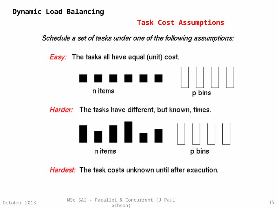
Task Cost Assumptions

MSc SAI - Parallel & Concurrent (J Paul Gibson) 16October 2013
Dynamic Load Balancing
Task Dependencies

MSc SAI - Parallel & Concurrent (J Paul Gibson) 17October 2013
Dynamic Load Balancing
Task Locality and Communication

MSc SAI - Parallel & Concurrent (J Paul Gibson) 18October 2013
Dynamic Load Balancing
Load balancing is well understood for parallel systems (message passing and shared memory) and there exists a wide range of solutions (both specific and generic).
You should know (at the minimum) about the simplest solutions One of the most common applications of load balancing is to provide a single Internet service from multiple servers, sometimes known as a server farm.
Commonly, load-balanced systems include popular web sites, large Internet Relay Chat networks, high-bandwidth File Transfer Protocol sites, Network News Transfer Protocol (NNTP) servers and Domain Name System (DNS) servers.
There are many open questions concerning load balancing for the cloud and for grids.

MSc SAI - Parallel & Concurrent (J Paul Gibson) 19October 2013
Static Load Balancing Problems --- Example 1
There is a 4 processor system where you have no prior knowledge of processor speeds.
You have a problem which is divided into 160 equivalent tasks.
Initial load balancing: distribute tasks evenly among processors.
After 10 seconds:• Processor 1 (P1) has finished• Processor P2 has 20 tasks completed• Processor P3 has 10 tasks completed• Processor P4 has 5 tasks complete
Question: what should we do?

MSc SAI - Parallel & Concurrent (J Paul Gibson) 20October 2013
Example 1 continued ...
We can do nothing ---
• Advantage: the simplest approach, just wait until all tasks are complete
• Disadvantage: P1 will remain idle until all other tasks are complete (and other processes may become idle)
Rebalance by giving some of the remaining tasks to P1 ---
• Advantage: P1 will no longer be idle
• Disadvantage: How do we rebalance in the best way?
Note: this question is not as simple as it first seems
MSc SAI - Parallel & Concurrent (J Paul Gibson) 21October 2013
Example 1 continued … some analysis
If we do not rebalance then we can predict execution time (time to complete all tasks) using the information we have gained through analysis of the execution times of our processors ---
P4 appears to be the slowest processor and data suggests that it completes 1 task every 2 seconds
Without re-balancing, we have to wait until the slowest processor (P4) has finished … 80 seconds in total.
Question: what fraction of total execution time is idle time?
Note: Without re-balancing we have too much idle time and have not reached optimum speed-up

MSc SAI - Parallel & Concurrent (J Paul Gibson) 22October 2013
Example 1 continued … some more analysis
The simplest re-balance:
when 1 processor has become idle then evenly distribute all tasks amongst all processors
So, in our example, after 10 seconds there are 85 tasks left to be completed (P2 has 20, P3 has 30, P4 has 35).
We divide evenly (or as evenly as possible) --- 85 = 4*21 +1
Thus, 3 processes take 21 tasks and 1 process takes 22 tasks.
Question: if we re-balance this time (but no other time) then what is the total execution time?

MSc SAI - Parallel & Concurrent (J Paul Gibson) 23October 2013
Example 1 continued … some more analysis
The simplest re-balance is therefore an improvement. However, we should be able to do better:•Why redistribute evenly?
• The processor speeds may vary greatly over time• The calculation is simple and no resources needed to store processor
history•Why not rebalance more than once?
• Re-balancing usually costs something• When only a few tasks are left its not worth the effort
Question: in the example, assuming the processors continue at the same speed, what is total execution time if we keep on re-balancing evenly when P1 becomes idle?

MSc SAI - Parallel & Concurrent (J Paul Gibson) 24October 2013
Re-balance Costs … example 1 revisited.
Question: If re-balancing costs:
• a) 50 seconds
• b) 20 seconds
• c) 5 seconds
then how many re-balancing operations should be performed in order to maximise the speed-up?
Re-balancing is an intuitive concept: if it is cheap do it, if it is expensive then don’t bother.
It is open to rigorous mathematical analysis: formalising the notion of cheap and expensive!

MSc SAI - Parallel & Concurrent (J Paul Gibson) 25October 2013
General re-balancing decision procedure
Based on a re-balancing graph, it is simple to automate the decision making process:
time
Tasks remaining
p1,p2,p3
p1,p2,p3
p1,p2,p3
balance balance balance balance
p1p1 p1
Here, p1 is the fastest processor and we perform 3 re-balances, which are very cheap!
We stop when re-balancing costs more than the time we gain!
MSc SAI - Parallel & Concurrent (J Paul Gibson) 26October 2013
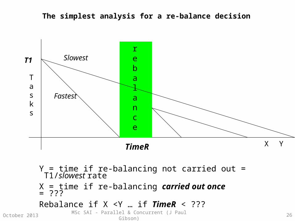
The simplest analysis for a re-balance decision
rebalance
TimeR
Fastest
Slowest
X Y
Y = time if re-balancing not carried out = T1/slowest rateX = time if re-balancing carried out once = ???Rebalance if X <Y … if TimeR < ???
Tasks
T1

MSc SAI - Parallel & Concurrent (J Paul Gibson) 27October 2013
The complete analysis for a re-balance decision
rebalance
TimeR
Fastest
Slowest
Y
Y = time if re-balancing not carried out = T1/slowest rateX = time if re-balancing carried out until (number of tasks < number of processes) = ???Rebalance if X <Y … if TimeR < ???
Tasks
T1rebalance
norebalance
X
MSc SAI - Parallel & Concurrent (J Paul Gibson) 28October 2013
Dynamic Load Balancing: Some further reading
Vipin Kumar, Ananth Y. Grama, and Nageshwara Rao Vempaty. 1994. Scalable load balancing techniques for parallel computers. J. Parallel Distrib. Comput. 22, 1 (July 1994)
M. H. Willebeek-LeMair and A. P. Reeves. 1993. Strategies for Dynamic Load Balancing on Highly Parallel Computers. IEEE Trans. Parallel Distrib. Syst. 4, 9 (September 1993)
G. Cybenko. 1989. Dynamic load balancing for distributed memory multiprocessors. J. Parallel Distrib. Comput. 7, 2 (October 1989)
Valeria Cardellini, Michele Colajanni, and Philip S. Yu. 1999. Dynamic Load Balancing on Web-Server Systems. IEEE Internet Computing 3, 3 (May 1999)
MSc SAI - Parallel & Concurrent (J Paul Gibson) 29October 2013
Parallelism Using Combinational Circuits
A combinational circuit is a family of models of computation –
• Number of inputs at one end• Number of outputs at the other end• Internally – a number of interconnected components arranged in columns
called stages• Each component can be viewed as a single processor with constant fan-in and
constant fan-out.• Components synchronise their computations (input to output) in a constant
time unit (independent of the input values)• Computations are usually simple logical operations (directly implementable in
hardware for speed!)• There must be no feedback

MSc SAI - Parallel & Concurrent (J Paul Gibson) 30October 2013
Combinational Circuits For List Processing
The best known examples of CCs are those for direct hardware implementation of list processing functions.
Fundamental operations of these hardware computers correspond to fundamental components.
Processing tasks which are non-fundamental on a standard single processor architecture can be parallelised (to reduce their complexity) by implementing them on a different parallel machine using a number of components set up in a combinational circuit.
Classic processing examples – searching, sorting, permuting, ….
But what are the useful components for implementation in a CC?
Parallelism Using Combinational Circuits
MSc SAI - Parallel & Concurrent (J Paul Gibson) 31October 2013
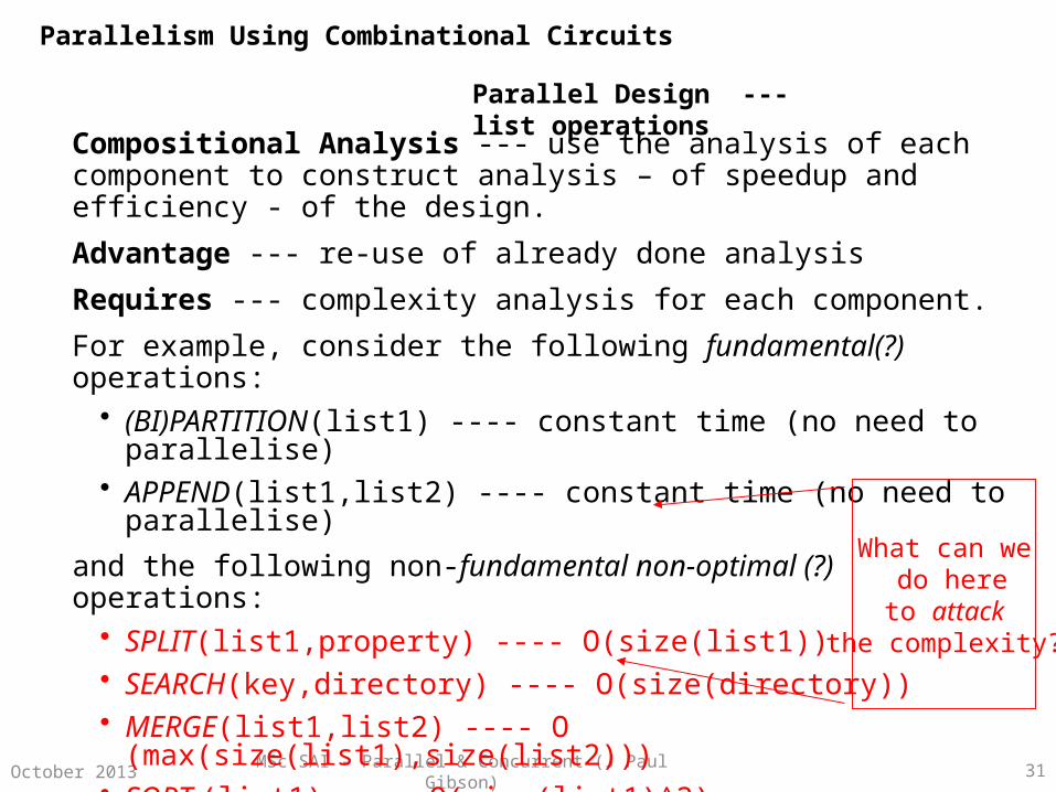
Parallel Design --- list operations
Compositional Analysis --- use the analysis of each component to construct analysis – of speedup and efficiency - of the design.
Advantage --- re-use of already done analysis
Requires --- complexity analysis for each component.
For example, consider the following fundamental(?) operations:• (BI)PARTITION(list1) ---- constant time (no need to parallelise)• APPEND(list1,list2) ---- constant time (no need to parallelise)
and the following non-fundamental non-optimal (?) operations:• SPLIT(list1,property) ---- O(size(list1)) • SEARCH(key,directory) ---- O(size(directory))• MERGE(list1,list2) ---- O (max(size(list1),size(list2)))• SORT (list1) ---- O(size(list1)^2)
What can we do here
to attack the complexity?
Parallelism Using Combinational Circuits

MSc SAI - Parallel & Concurrent (J Paul Gibson) 32October 2013
Parallel Design ---the split operation
Question: how to parallelise the split operation?
Answer: depends if the property is structured!
Consider:
SPLIT(property)
Where: split partitions L into M and N -
•Forall Mx, Property(Mx)
•Forall Ny, Not(Property(Ny))
•Append(M,N) is a permutation of L
Question: Can we use the structure in the Property to help parallelise the design? EXAMPLE: A ^ B, A v B, ‘any boolean expression’
L1
.
.
.
Ln
M1
.
.
Mp
N1..Nq
Parallelism Using Combinational Circuits

MSc SAI - Parallel & Concurrent (J Paul Gibson) 33October 2013
Example: Splitting on property A ^ B
app
SPLIT(B)SPLIT(A)
BIP
SPLIT(B)
appapp
SPLIT(A)
app
Question: what do/could we gain?
Question: what about splitting on property AVB?
bipartitionappend
Parallelism Using Combinational Circuits
MSc SAI - Parallel & Concurrent (J Paul Gibson) 34October 2013
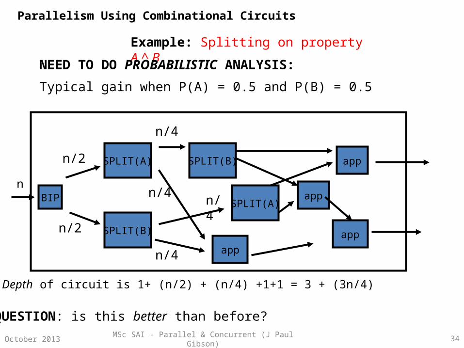
Example: Splitting on property A ^ B
app
SPLIT(B)SPLIT(A)
BIP
SPLIT(B)
appapp
SPLIT(A)
app
NEED TO DO PROBABILISTIC ANALYSIS:
Typical gain when P(A) = 0.5 and P(B) = 0.5
n
n/2
n/2
n/4
n/4 n/4
n/4
Depth of circuit is 1+ (n/2) + (n/4) +1+1 = 3 + (3n/4)
QUESTION: is this better than before?
Parallelism Using Combinational Circuits

MSc SAI - Parallel & Concurrent (J Paul Gibson) 35October 2013
Split example on non-structured property
EXAMPLE: Split an input integer list into evens and odds
Question: what is average speedup for the following design?
BIP
SPLIT
SPLIT
app
app
Parallelism Using Combinational Circuits

MSc SAI - Parallel & Concurrent (J Paul Gibson) 36October 2013
Split example on non-structured property
Question: what is average speedup for the following design?
ANSWER: do Probabilistic Analysis as before … Depth = 2+ n/2
BIP
SPLIT(even/odd)
SPLIT(even/odd)
app
appn
n/2
n/2n/4
n/4
n/4
n/4
n/2
n/2
Parallelism Using Combinational Circuits
MSc SAI - Parallel & Concurrent (J Paul Gibson) 37October 2013
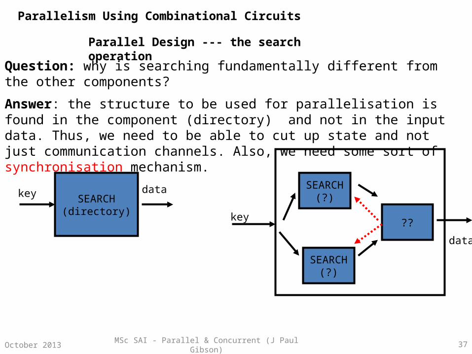
Parallel Design --- the search operation
Question: why is searching fundamentally different from the other components?
Answer: the structure to be used for parallelisation is found in the component (directory) and not in the input data. Thus, we need to be able to cut up state and not just communication channels. Also, we need some sort of synchronisation mechanism.
SEARCH(directory)
SEARCH(?)
??
SEARCH(?)key data
key
data
Parallelism Using Combinational Circuits
MSc SAI - Parallel & Concurrent (J Paul Gibson) 38October 2013
Sorting by Merging
•A good example of recursively constructing combinational circuits(CC)
•The same technique can be applied to all CC’s synthesis and analysis
•Requires understanding of a standard non-parallel (sequential) algorithm
•Shows that some sequential algorithms are better suited to parallel
implementation than others
•Best suited to formal reasoning (preconditions, invariants, induction …)
Parallelism Using Combinational Circuits

MSc SAI - Parallel & Concurrent (J Paul Gibson) 39October 2013
Merging --- the base case
Merge 2 sorted sequences of equal length m = 2^n.
Base case, n=0 => m = 1.
Precondition is met since a list with only 1 element is already sorted!
The component required is actually a comparison operator
Merge(1) = Compare
C (or CAE)
X= [x1]
Y = [y1]
[min (x1,y1)]
[max (x1,y1)]
M1
Uesful Measures: Width = 1 Depth = 1 Size = 1
Parallelism Using Combinational Circuits

MSc SAI - Parallel & Concurrent (J Paul Gibson) 40October 2013
Merge --- the first recursive composition
QUESTION:
Using only component M1 (the comparison C), how can we construct a circuit for merging lists of length 2 (M2)?
ANALYSIS:
•How many M1s … the size … are needed in total?
•What is the complexity … based on the depth?
•During execution what is our most efficient use of parallel resources … based on width?
Parallelism Using Combinational Circuits
MSc SAI - Parallel & Concurrent (J Paul Gibson) 41October 2013
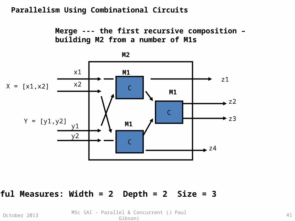
Merge --- the first recursive composition – building M2 from a number of M1s
C
C
C
X = [x1,x2]
x1
x2
y1y2
Y = [y1,y2]
z1
z2
z3
z4
Useful Measures: Width = 2 Depth = 2 Size = 3
M2
M1
M1
M1
Parallelism Using Combinational Circuits

MSc SAI - Parallel & Concurrent (J Paul Gibson) 42October 2013
Proving M2 to be correct
Validation ---We can test the circuit with different input values for X and YBut, this does not prove that the circuit is correct for all possible casesClearly, there are equivalence classes of testsWe want to identify all such classes and prove correctness for the classes.As the number of classes are finite, we can use an automated prover to do thisComplete proof of all equivalence classes => system is verified.Here we have 6 equivalence classes (or 3,if we note the symmetry in swapping X and Y)
DISJOINT OVERLAP CONTAINMENT
x1 x2 y1 y2x1
y1
x2
y2
x1
y1 y2
x2
Parallelism Using Combinational Circuits
MSc SAI - Parallel & Concurrent (J Paul Gibson) 43
M2
The next recursive step --- M4
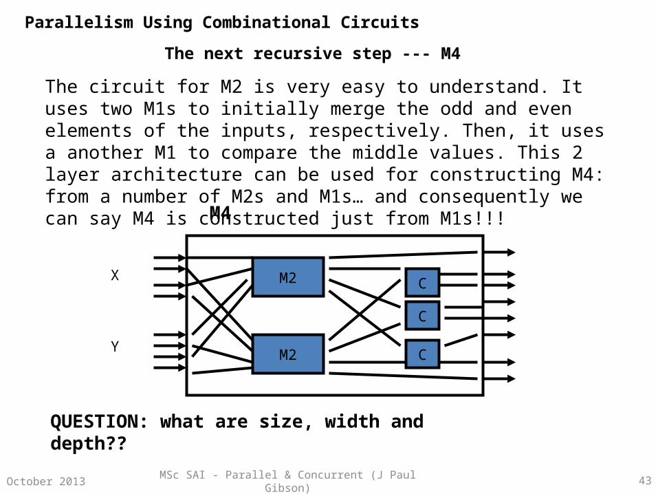
The circuit for M2 is very easy to understand. It uses two M1s to initially merge the odd and even elements of the inputs, respectively. Then, it uses a another M1 to compare the middle values. This 2 layer architecture can be used for constructing M4: from a number of M2s and M1s… and consequently we can say M4 is constructed just from M1s!!!
M2
C
C
C
X
Y
QUESTION: what are size, width and depth??
M4
October 2013
Parallelism Using Combinational Circuits

MSc SAI - Parallel & Concurrent (J Paul Gibson) 44October 2013
M2
The next recursive step --- M4
M2
C
C
C
X
Y
Depth = 3 Width = 4 Size = 9
M4
Depth (M4) = Depth (M2) +1Width (M4) = Max (2*Width(M2), 3)Size (M4) = 2*Size(M2) + 3
Parallelism Using Combinational Circuits
MSc SAI - Parallel & Concurrent (J Paul Gibson) 45October 2013
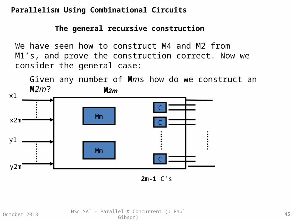
The general recursive construction
We have seen how to construct M4 and M2 from M1’s, and prove the construction correct. Now we consider the general case:
Given any number of Mms how do we construct an M2m?
Mm
Mm
M2m
C
C
C
2m-1 C’s
x1
x2m
y1
y2m
Parallelism Using Combinational Circuits
MSc SAI - Parallel & Concurrent (J Paul Gibson) 46October 2013
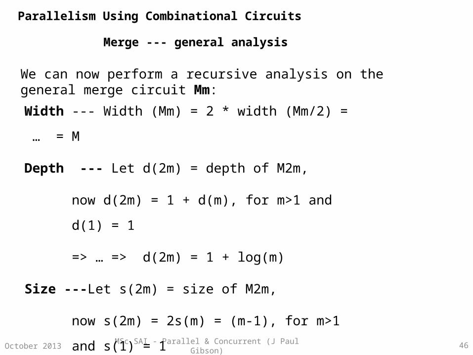
Merge --- general analysis
We can now perform a recursive analysis on the general merge circuit Mm:
Width --- Width (Mm) = 2 * width (Mm/2) = … = M
Depth --- Let d(2m) = depth of M2m,
now d(2m) = 1 + d(m), for m>1 and d(1) = 1
=> … => d(2m) = 1 + log(m)
Size ---Let s(2m) = size of M2m,
now s(2m) = 2s(m) = (m-1), for m>1 and s(1) = 1
=> … => s(2m) = 1 + mlog(m)
Parallelism Using Combinational Circuits

MSc SAI - Parallel & Concurrent (J Paul Gibson) 47October 2013
Sorting by Merging
We can use the merge circuits to sort arrays ---
For example, sorting an array of 8 numbers:
M1
M1
M1
M1
M2
M2
M4
Proof of correctness --- try to sketch the proof in your own time
S8
Parallelism Using Combinational Circuits

MSc SAI - Parallel & Concurrent (J Paul Gibson) 48October 2013
Sorting by Merging – the analysis
•Analyse the base case for sorting a 2 integer list (S2).
•Synthesise and analyse S4
•What are the width, depth and size of Sn?
•What about cases when n is not a power of 2?
Question: is there a more efficient means of sorting using the merge components? If so, why?
To DO: Look for information on parallel sorting on the web
Parallelism Using Combinational Circuits

MSc SAI - Parallel & Concurrent (J Paul Gibson) 49October 2013
Permutation Circuits
An important function in computer science is to apply an arbitrary permutation to an array.
We consider arrays of length m (m = 2^n) and perform a recursive composition.
First, an example:Permute x1,x2,x3,x4,x5,x6,x7,x8 to x5,x4,x3,x1,x8,x7,x6,x2
The circuit can be shown as the following box:x1
x8
Question:
what goes inside?
x5x4x3x1x8x7x6x2
Parallelism Using Combinational Circuits

MSc SAI - Parallel & Concurrent (J Paul Gibson) 50October 2013
The simplest permutation --- a switchThe base case is to permute an input array of 2 elements
(a wire suffices for 1 element!)
SWITCH
A switch has two possible states --- off or on.
A switch is therefore a programmable permutation circuit for input arrays of length 2.
We use the notation P2 to denote a switch.
Question: how can we re-use the switch to produce a a P4?
Question: how can we re-use a Pn to produce a P2n?
Parallelism Using Combinational Circuits

MSc SAI - Parallel & Concurrent (J Paul Gibson) 51October 2013
Constructing P4 from P2s
The following circuit implements a P4 ---
P2
P2
P2
P2
P2
Input Centre Output
Question:
can you verify that this is correct?
Parallelism Using Combinational Circuits

MSc SAI - Parallel & Concurrent (J Paul Gibson) 52October 2013
Programming the P4
•To program P4 we just start at the required ouputs and hardwire the
switches to give correct paths.
•Note, programming is not unique for all permutations.
•N=4 => number of permutations = 4! = 24
•Number of switches = 5 =>2 ^5 (=32) different programs.
•Thus , the number of programs is more than the number of permutations.
•Can we prove that the P4 is complete --- all permutations are
programmable
•Since the number (in P4) is finite, we can prove it exhaustively with a tool.
•We can use induction to prove it in the general case.
Parallelism Using Combinational Circuits

MSc SAI - Parallel & Concurrent (J Paul Gibson) 53October 2013
Programming P4 to give permutation 2,1,4,3
The following program (see right) implements a P4 (2,1,4,3) ---
S1
S2
S4
S3
S5
Input Centre Output
12
3
4
2
1
4
3
S1 = on
S2 = on
S3 = off
S4 = off
S5 = off
Question: is this a unique program? If not, find a permutation which is.
Parallelism Using Combinational Circuits
MSc SAI - Parallel & Concurrent (J Paul Gibson) 54October 2013
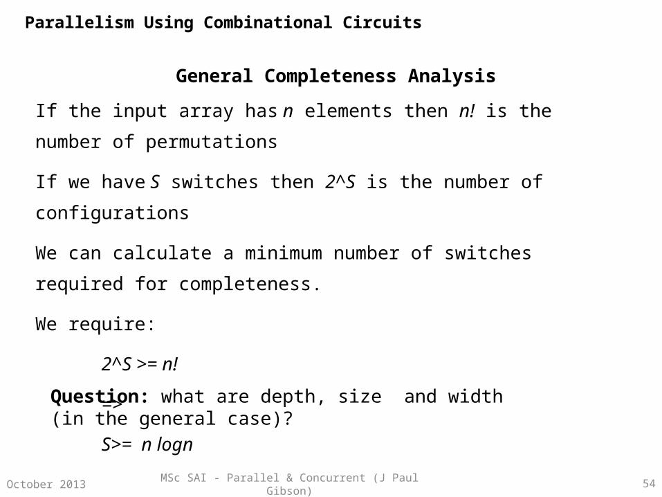
General Completeness Analysis
If the input array has n elements then n! is the number of permutations
If we have S switches then 2^S is the number of configurations
We can calculate a minimum number of switches required for completeness.
We require:
2^S >= n!
=>
S>= n logn
Question: what are depth, size and width (in the general case)?
Parallelism Using Combinational Circuits

MSc SAI - Parallel & Concurrent (J Paul Gibson) 55October 2013
Constructing a P8 using 2 P4s and some switches (P2s)
Input Centre Output
Parallelism Using Combinational Circuits
MSc SAI - Parallel & Concurrent (J Paul Gibson) 56October 2013
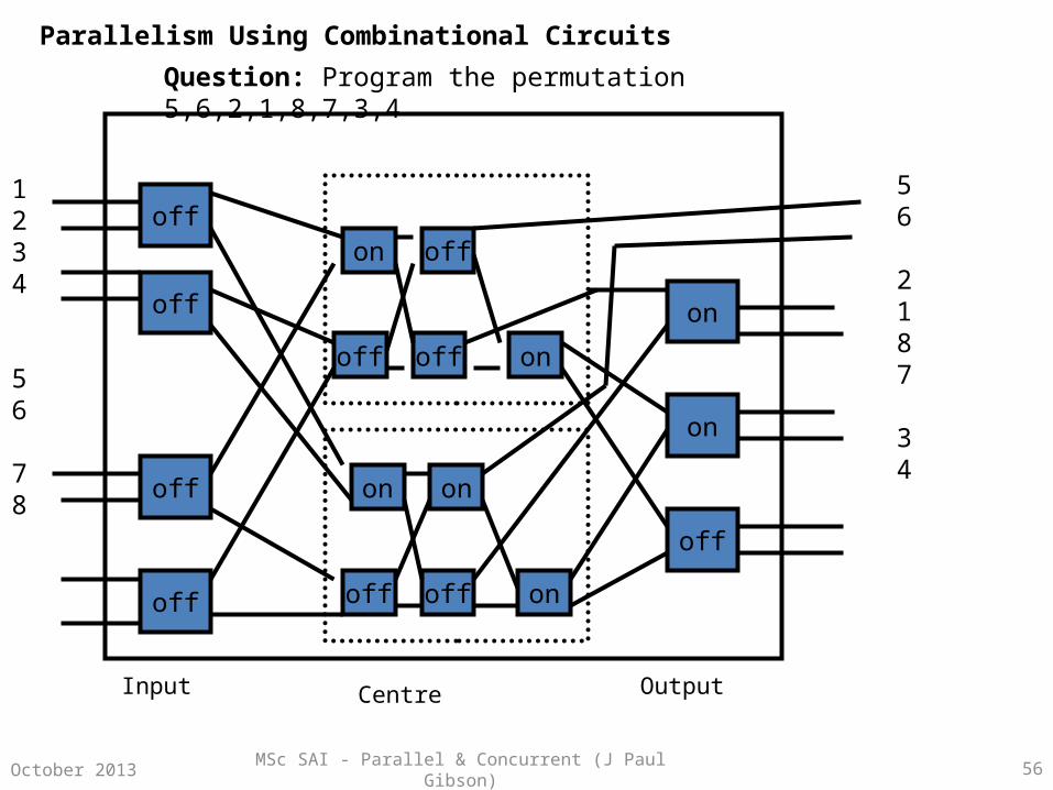
Question: Program the permutation 5,6,2,1,8,7,3,4
off
off
off
off
off
on
on
on
off off on
off
on
off off on
on
Input Centre Output
1234
56
78
56
2187
34
Parallelism Using Combinational Circuits
MSc SAI - Parallel & Concurrent (J Paul Gibson) 57October 2013
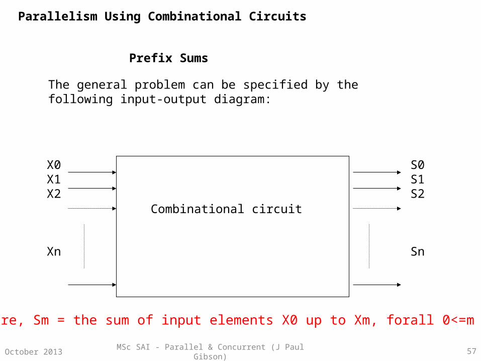
Prefix Sums
The general problem can be specified by the following input-output diagram:
X0X1X2
Xn
S0S1S2
Sn
Combinational circuit
Where, Sm = the sum of input elements X0 up to Xm, forall 0<=m <= n
Parallelism Using Combinational Circuits

MSc SAI - Parallel & Concurrent (J Paul Gibson) 58October 2013
Prefix Sums
X0X1X2
Xn
S0S1S2
Sn
Combinational circuit
Question: what is the fundamental building block?
FOR YOU TO TRY – Design a recursive combinational circuit and analyse complexity issues.
Question: is your design optimal?
Parallelism Using Combinational Circuits

MSc SAI - Parallel & Concurrent (J Paul Gibson) 59October 2013
Parallelism Using Combinational Circuits: Further Reading
C. D. Thompson. 1983. The VLSI Complexity of Sorting. IEEE Trans. Comput. 32, 12 (December 1983)
Richard E. Ladner and Michael J. Fischer. 1980. Parallel Prefix Computation. J. ACM 27, 4 (October 1980)
R. P. Brent and H. T. Kung. 1982. A Regular Layout for Parallel Adders. IEEE Trans. Comput. 31, 3 (March 1982)
MSc SAI - Parallel & Concurrent (J Paul Gibson) 60October 2013
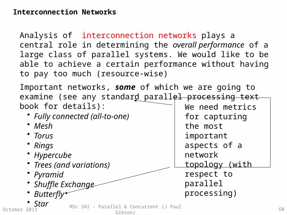
Interconnection Networks
Analysis of interconnection networks plays a central role in determining the overall performance of a large class of parallel systems. We would like to be able to achieve a certain performance without having to pay too much (resource-wise)
Important networks, some of which we are going to examine (see any standard parallel processing text book for details):
• Fully connected (all-to-one)• Mesh• Torus• Rings• Hypercube• Trees (and variations)• Pyramid• Shuffle Exchange• Butterfly• Star
We need metrics for capturing the most important aspects of a network topology (with respect to parallel processing)

MSc SAI - Parallel & Concurrent (J Paul Gibson) 61October 2013
Metrics for Interconnection Networks
•Degree: The degree of a processor is the number of its (direct) neighbours in the network. The degree of a network is the maximum of all processor degrees in the network. A high degree has high theoretical power but a low degree is more practical.
•Connectivity: Network nodes and links sometimes fail and must be removed from service for repair. When components fail the network should continue to function with reduced capacity. The node connectivity is the minimum number of nodes that must be removed in order to partition (divide) the network. The link connectivity is the minimum number of links that must be removed in order to partition the network
•Diameter: The diameter of a network is the maximum inter-node distance -- the maximum number of nodes that must be traversed to send a message to any node along a shortest path. Lower diameter implies shorter time to send messages across network.
Interconnection Networks

MSc SAI - Parallel & Concurrent (J Paul Gibson) 62October 2013
Metrics for Interconnection Networks (continued)
•Narrowness: This is a measure of (potential) congestion.
Partition the network into 2 groups of processors (A and B, say). In each group the number of processors is noted as Na and Nb (Nb<=Na). Count the number of interconnections between A and B (call this I). The maximum value of Nb/I for all possible partitions is the narrowness.
•Expansion increments: This is a measure of (potential) expansion
A network should be expandable --- it should be possible to create larger systems (of the same topology) by simply adding new nodes. It is better (why?) to have the option of small increments.
Interconnection Networks
MSc SAI - Parallel & Concurrent (J Paul Gibson) 63October 2013
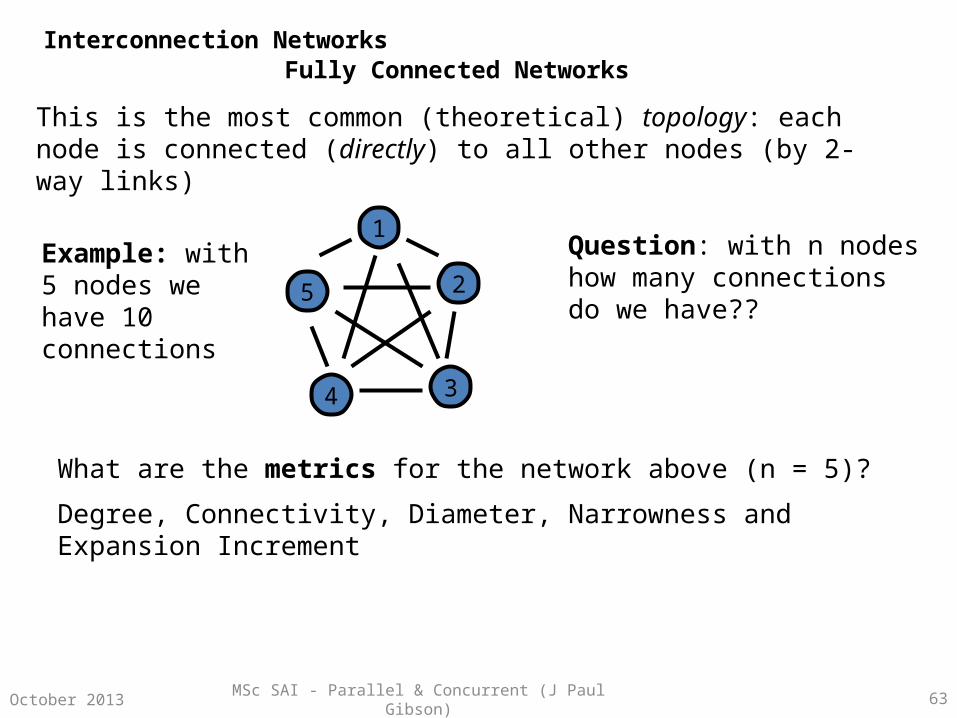
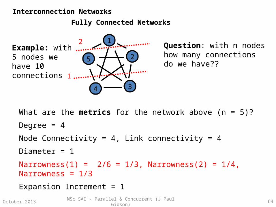
Fully Connected Networks
This is the most common (theoretical) topology: each node is connected (directly) to all other nodes (by 2-way links)
1
2
34
5
Example: with 5 nodes we have 10 connections
Question: with n nodes how many connections do we have??
What are the metrics for the network above (n = 5)?
Degree, Connectivity, Diameter, Narrowness and Expansion Increment
Interconnection Networks
MSc SAI - Parallel & Concurrent (J Paul Gibson) 64October 2013
Fully Connected Networks
1
2
34
5
Example: with 5 nodes we have 10 connections
Question: with n nodes how many connections do we have??
What are the metrics for the network above (n = 5)?
Degree = 4
Node Connectivity = 4, Link connectivity = 4
Diameter = 1
Narrowness(1) = 2/6 = 1/3, Narrowness(2) = 1/4, Narrowness = 1/3
Expansion Increment = 1
1
2
Interconnection Networks
MSc SAI - Parallel & Concurrent (J Paul Gibson) 65October 2013
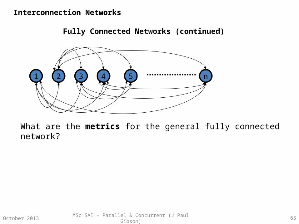
Fully Connected Networks (continued)
41 52 3
What are the metrics for the general fully connected network?
n
Interconnection Networks
MSc SAI - Parallel & Concurrent (J Paul Gibson) 66October 2013
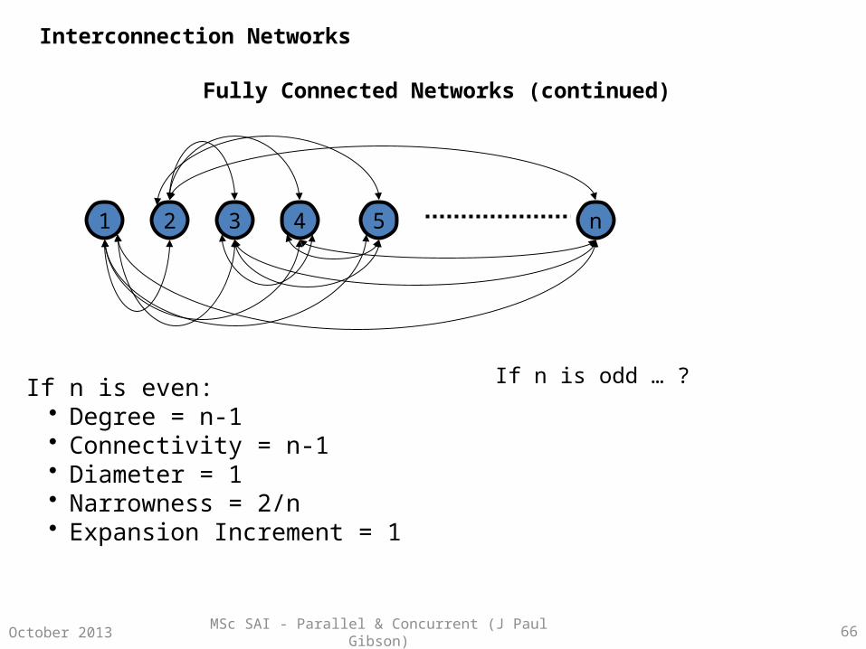
Fully Connected Networks (continued)
41 52 3 n
If n is even:• Degree = n-1• Connectivity = n-1• Diameter = 1• Narrowness = 2/n• Expansion Increment = 1
If n is odd … ?
Interconnection Networks
MSc SAI - Parallel & Concurrent (J Paul Gibson) 67October 2013
A Mesh Network
One of the most common topologies
In a mesh, the nodes are arranged in a k-dimensional lattice of width w, giving a total of w^k nodes.
Usually,
• k =1 …giving a linear array, or
• k =2 …. Giving a 2-dimensional matrix
Communication is allowed only between neighbours (no ‘diagonal connections’)
A mesh with wraparound is called a torus
Interconnection Networks

MSc SAI - Parallel & Concurrent (J Paul Gibson) 68October 2013
A linear array
Example: a 1-D mesh of width 4 with no wraparound on ends
Question: what are degrees of centre and end nodes?
Question: what are the metrics for the linear array, above?
Question: what are the metrics in the general case?
Interconnection Networks
MSc SAI - Parallel & Concurrent (J Paul Gibson) 69October 2013
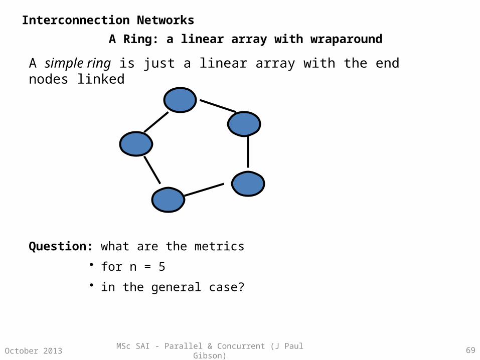
A Ring: a linear array with wraparound
A simple ring is just a linear array with the end nodes linked
Question: what are the metrics
• for n = 5
• in the general case?
Interconnection Networks
MSc SAI - Parallel & Concurrent (J Paul Gibson) 70October 2013
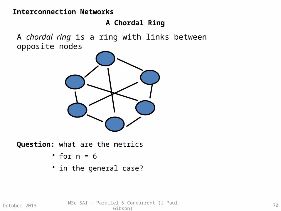
A Chordal Ring
A chordal ring is a ring with links between opposite nodes
Question: what are the metrics
• for n = 6
• in the general case?
Interconnection Networks
MSc SAI - Parallel & Concurrent (J Paul Gibson) 71October 2013
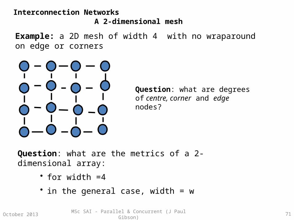
A 2-dimensional mesh
Example: a 2D mesh of width 4 with no wraparound on edge or corners
Question: what are degrees of centre, corner and edge nodes?
Question: what are the metrics of a 2-dimensional array:
• for width =4
• in the general case, width = w
Interconnection Networks

MSc SAI - Parallel & Concurrent (J Paul Gibson) 72October 2013
A 2-dimensional torus (mesh with wraparound)
Example: a 2D mesh of width 4 with wraparound on opposite corners
Question: what are the metrics of such an 2-dimensional torus:
• for width =4
• in the general case, width = w
Interconnection Networks

MSc SAI - Parallel & Concurrent (J Paul Gibson) 73October 2013
A 3-dimensional torus (width =3)
Example:
Question: what are the metrics of such an 3-dimensional torus:
Interconnection Networks
MSc SAI - Parallel & Concurrent (J Paul Gibson) 74October 2013
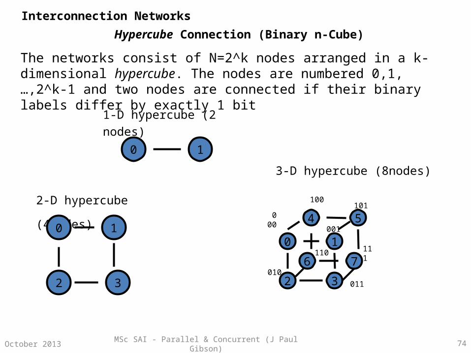
Hypercube Connection (Binary n-Cube)
The networks consist of N=2^k nodes arranged in a k-dimensional hypercube. The nodes are numbered 0,1,…,2^k-1 and two nodes are connected if their binary labels differ by exactly 1 bit
2-D hypercube (4nodes)
0 1
00
1
32
1
2 3
6
4 5
7
000
010011
111
101100
001
110
1-D hypercube (2 nodes)
3-D hypercube (8nodes)
Interconnection Networks

MSc SAI - Parallel & Concurrent (J Paul Gibson) 75October 2013
4-D HyperCube (binary 4 cube)
A K-dimensional hypercube is formed by combining two K-1 dimensional hypercubes and connecting corresponding nodes (recursively).
Question: what are the metrics of an n-dimensional hypercube?
Interconnection Networks
MSc SAI - Parallel & Concurrent (J Paul Gibson) 76October 2013
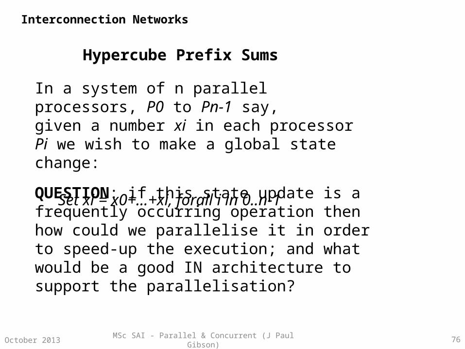
Hypercube Prefix Sums
In a system of n parallel processors, P0 to Pn-1 say,given a number xi in each processor Pi we wish to make a global state change:
Set xi = x0+…+xi, forall i in 0..n-1
QUESTION: if this state update is a frequently occurring operation then how could we parallelise it in order to speed-up the execution; and what would be a good IN architecture to support the parallelisation?
Interconnection Networks
MSc SAI - Parallel & Concurrent (J Paul Gibson) 77October 2013
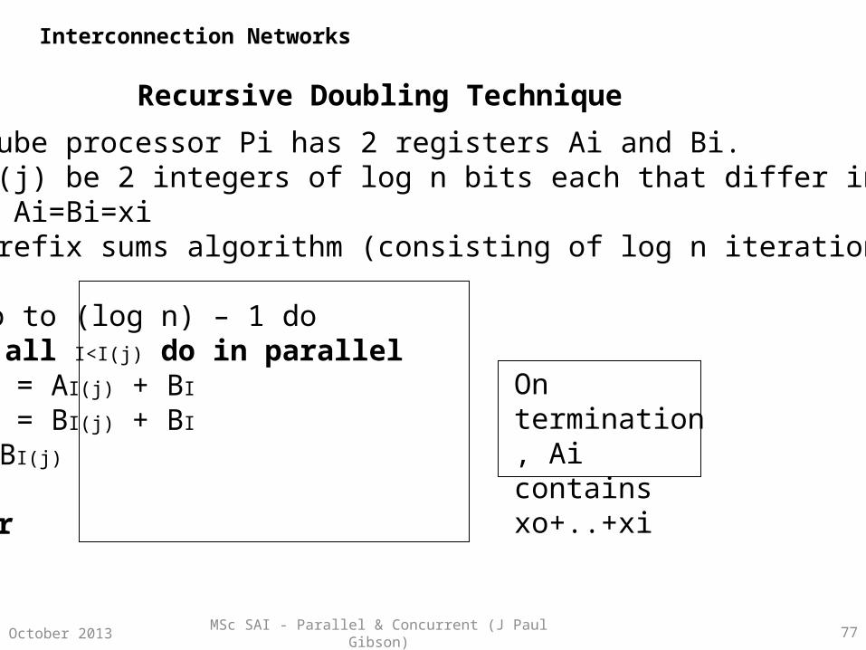
Recursive Doubling Technique
Each hypercube processor Pi has 2 registers Ai and Bi.Let I and I(j) be 2 integers of log n bits each that differ in the jth bitInitialise, Ai=Bi=xiApply the prefix sums algorithm (consisting of log n iterations):
for j = o to (log n) – 1 do for all I<I(j) do in parallel
AI(j) = AI(j) + BI
BI(j) = BI(j) + BI
BI = BI(j) endfor
endfor
On termination, Ai contains xo+..+xi
Interconnection Networks
MSc SAI - Parallel & Concurrent (J Paul Gibson) 78October 2013
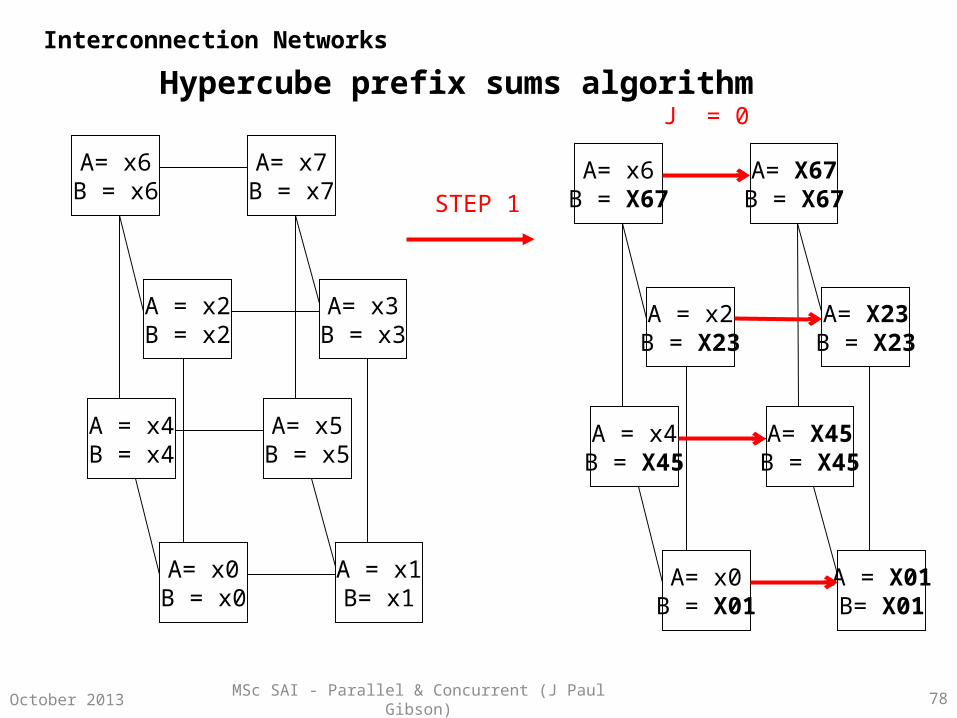
Hypercube prefix sums algorithm
A= x6B = x6
A= x7B = x7
A = x2B = x2
A= x3B = x3
A = x4B = x4
A= x5B = x5
A= x0B = x0
A = x1B= x1
A= x6B = X67
A= X67B = X67
A = x2B = X23
A= X23B = X23
A = x4B = X45
A= X45B = X45
A= x0B = X01
A = X01B= X01
STEP 1
J = 0
Interconnection Networks

MSc SAI - Parallel & Concurrent (J Paul Gibson) 79October 2013
A= X46B = X47
A= X47B = X47
A = X02B = X03
A= X03B = X03
A = x4B = X47
A= X45B = X47
A= x0B = X03
A = X01B= X03
STEP 2
A= x6B = X67
A= X67B = X67
A = x2B = X23
A= X23B = X23
A = x4B = X45
A= X45B = X45
A= x0B = X01
A = X01B= X01
J = 0 J = 1
Interconnection Networks
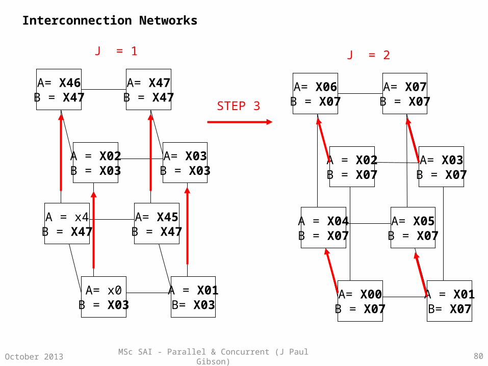
MSc SAI - Parallel & Concurrent (J Paul Gibson) 80October 2013
A= X06B = X07
A= X07B = X07
A = X02B = X07
A= X03B = X07
A = X04B = X07
A= X05B = X07
A= X00B = X07
A = X01B= X07
J = 1 J = 2
A= X46B = X47
A= X47B = X47
A = X02B = X03
A= X03B = X03
A = x4B = X47
A= X45B = X47
A= x0B = X03
A = X01B= X03
STEP 3
Interconnection Networks
MSc SAI - Parallel & Concurrent (J Paul Gibson) 81October 2013
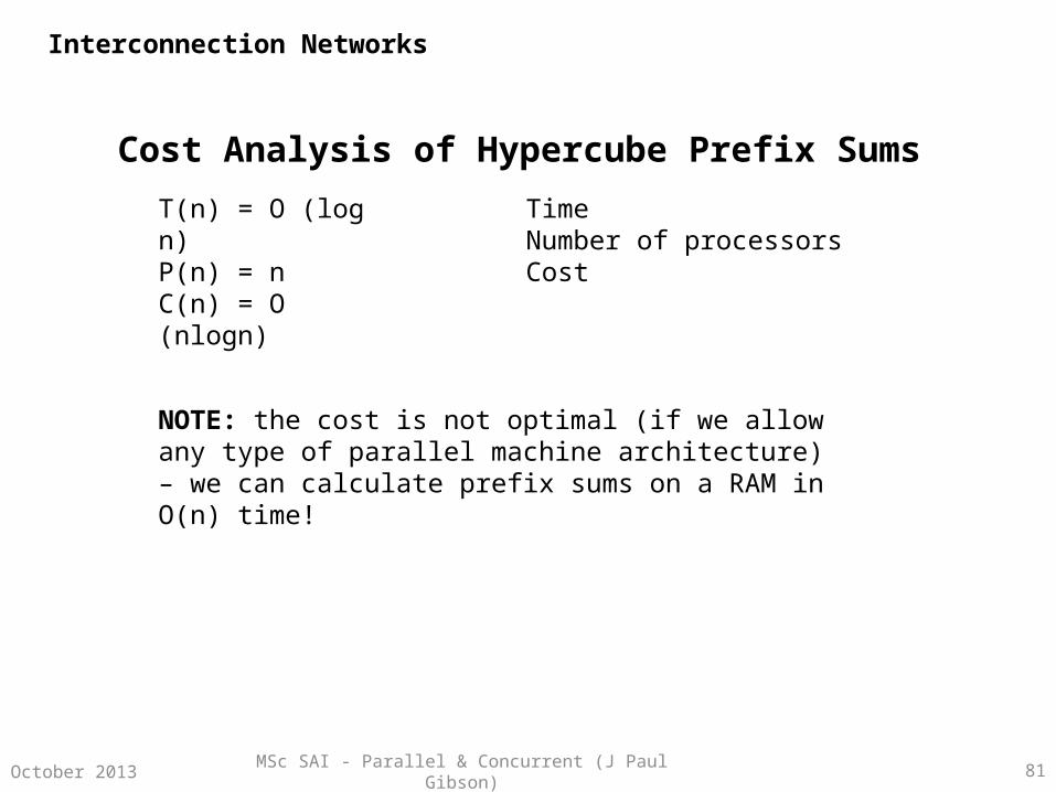
Cost Analysis of Hypercube Prefix Sums
T(n) = O (log n) P(n) = nC(n) = O (nlogn)
TimeNumber of processorsCost
NOTE: the cost is not optimal (if we allow any type of parallel machine architecture) – we can calculate prefix sums on a RAM in O(n) time!
Interconnection Networks

MSc SAI - Parallel & Concurrent (J Paul Gibson) 82October 2013
Processor TreeThe standard model is for the processors to form a complete binary tree:
• has d levels (0 .. d-1)
• Number of nodes = 2^d -1
• metrics = ...? Level
2
1
0
root
leaves
Interconnection Networks

MSc SAI - Parallel & Concurrent (J Paul Gibson) 83October 2013
Tree variationsThere are many variations on the tree topology:
• mesh of trees
• tree of meshes
• tree of rings
• ring of trees
• etc ...
Note: you will be expected to be able to formulate the metrics for these types of synthesised topologies
Interconnection Networks

MSc SAI - Parallel & Concurrent (J Paul Gibson) 84October 2013
Pyramid Construction
A 1-dimensional pyramid parallel computer is obtained by adding 2-way links connecting processors at the same level in a binary tree, thus forming a linear array at each level.
Question: what are metrics of such a pyramid of dimension = 1?
A 2-dimensional pyramid consists of (4^(d+1)-1)/ 3 processors distributed among d+1 levels. All processors at the same level are connected together to form a mesh. At level d, there is 1 processor -- the apex. In general, a processor at level I, in addition to being connected to its four neighbours at the same level, has connections to four children at level I-1 (provided I>=1) and to one parent at level I+1 (provided I<=d-1).
Question: what are metrics for a pyramid (d=2)? …
what does it look like???
Interconnection Networks

MSc SAI - Parallel & Concurrent (J Paul Gibson) 85October 2013
Shuffle Exchange
Question: can you reverse engineer the definition of a perfect shuffle exchange from looking at the one above??
p0 p2 p5p1 p3 p4 p6 p7
This is a perfect 8-processor shuffle exchange
Interconnection Networks

MSc SAI - Parallel & Concurrent (J Paul Gibson) 86October 2013
Shuffle Exchange
p0 p2 p5p1 p3 p4 p6 p7
A 1-way communication line links PI to PJ, where:
• J= 2I for 0<=I<=4-1,
• J = 2I+1-8 for 4<=I<=N-1
2-way links are added to every even numbered processor and its successor
Interconnection Networks

MSc SAI - Parallel & Concurrent (J Paul Gibson) 87October 2013
Shuffle Exchange
p0 p2 p5p1 p3 p4 p6 p7
This corresponds to a perfect shuffle (like a deck of cards)
Reversing the direction of the links gives a perfect-unshuffle
Question: what are metrics for
• case n=8 and general case for any n which is a power of 2?
Interconnection Networks
MSc SAI - Parallel & Concurrent (J Paul Gibson) 88October 2013
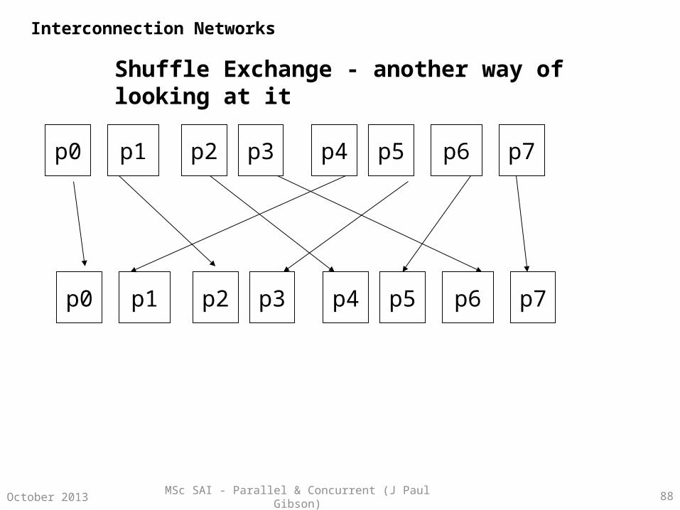
Shuffle Exchange - another way of looking at it
p0 p2 p5p1 p3 p4 p6 p7
p0 p2 p5p1 p3 p4 p6 p7
Interconnection Networks
MSc SAI - Parallel & Concurrent (J Paul Gibson) 89October 2013
Cube-connected cycles
Begin with a q-dim hypercube and replace each of its 2^q corners with a ring of q processors.
Each processor in a ring is connected to a processor in a neighbouring ring in the same dimension
Number of processors is N = 2^q * q.
QUESTION: can you draw this for q = 3 ???
QUESTION: can you calculate the network metrics??
Interconnection Networks

MSc SAI - Parallel & Concurrent (J Paul Gibson) 90October 2013
3-dim cube connected cycle
Interconnection Networks

MSc SAI - Parallel & Concurrent (J Paul Gibson) 91October 2013
StarSize property:
for any given integer m, each processor corresponds to a distinct permutation of m symbols.
Thus, the network connects N=m! processors.
Connection property:
Pv is connected to Pu iff the index u can be obtained from v by exchanging the first symbol with the ith symbol, where 2 <=i<=m
Example:
m=4, if v = 2134 and u = 3124 then Pu and Pv are connected by a 2-way link since 3124 and 2134 can be obtained from one another by exchanging the 1st and 3rd symbols
QUESTION: can you draw this for m = 4 ??
Interconnection Networks

MSc SAI - Parallel & Concurrent (J Paul Gibson) 92October 2013
Star: m = 41234
2314 3124
21343214
1324
4231
2341 3421
24313241
4321
2413
1243 4123
14234213
2143
3412
1342 4132
14324312
3142
Question:
•diameter
•connectivity
•narrowness
•expansion increment??
Interconnection Networks

MSc SAI - Parallel & Concurrent (J Paul Gibson) 93October 2013
Designing an Interconnection Network
Typically, requirements will be specified as bounds on a subset of metrics, eg:
• minn < number nodes < maxn
• minl < number links < maxl
• connectivity > cmin
• diameter < dmax
• narrowness < nmax
Normally, your experience will tell you if a classic IN fits the bill. Otherwise you will refine an IN which is close to meeting the requirements; or combine 2 (or more) in a complementary fashion… This is not always easy/possible!
Interconnection Networks

MSc SAI - Parallel & Concurrent (J Paul Gibson) 94October 2013
Algorithms and Interconnection Networks
The applications to which a parallel computer is destined – as well as the metrics – also play an important role in its selection:
• Meshes for matrices• Trees for data search• Hypercube for flexibility
To understand the engineering choices and compromises we really need to look at other examples.
Interconnection Networks

MSc SAI - Parallel & Concurrent (J Paul Gibson) 95October 2013
Some Further ReadingInterconnection Networks
Tse-yun Feng. 1981. A Survey of Interconnection Networks. Computer 14, 12 (December 1981), 12-27.
William J. Dally and Brian Towles. 2001. Route packets, not wires: on-chip inteconnection networks. In Proceedings of the 38th annual Design Automation Conference (DAC '01). ACM, New York, NY, USA, 684-689.
D. P. Agrawal. 1983. Graph Theoretical Analysis and Design of Multistage Interconnection Networks. IEEE Trans. Comput. 32, 7 (July 1983), 637-648.
MSc SAI - Parallel & Concurrent (J Paul Gibson) 96October 2013
Some More FundamentalsWith N processors, each with its own data stream it isusually necessary to communicate results between processors.
Two standard methods ---Shared memory ----> communication by shared variablesInterconnection Network ---> communication by message passing
Hybrid Designs --- combine the 2 standard methods
Question: why do we say usually ??
Question: is there any theoretic difference between the 2 methods ---
can we implement each method using the other? What about complexity rather than computability?
Shared Memory

MSc SAI - Parallel & Concurrent (J Paul Gibson) 97October 2013
Shared Memory
Pn
P1
P2P3
P4 Memory
Global address space is accessible by all processors
Communication Pi ---> Pj ???
Pi writes to address(x) and Pj reads from address(x)
Advantages --- communication is simple
Disadvantages --- introduces non-determinism from race conditions

MSc SAI - Parallel & Concurrent (J Paul Gibson) 98October 2013
Shared Memory: More General Model
Pm
P1
P2P3
P4 Memory
There is a structure to sharing, enforcing scope like in programming languages
Pm
Pm+1
Pm+2Pm+3
Pm+4Memory
Memory

MSc SAI - Parallel & Concurrent (J Paul Gibson) 99October 2013
Non-determinism Example ---
Shared memory x=0
P1: x:=x+1 P2: x:= x+2
Process Q = P1¦¦¦ P3 ---
P1 and P2 running in parallel with no synchronisation
Question: x = ??? when Q has finished execution
Answer: x can be 1,2 or 3 depending on interleaving of read/write events during assignment to variable x.
Problem occurs because, in general, assignment is not an atomic event
Shared Memory
MSc SAI - Parallel & Concurrent (J Paul Gibson) 100October 2013
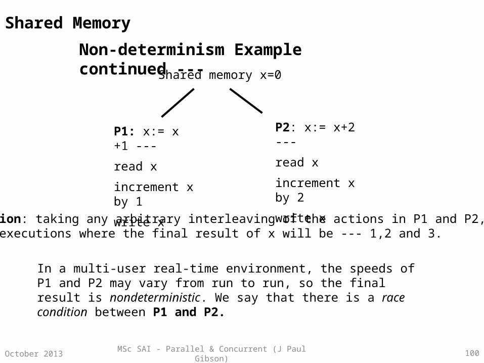
Non-determinism Example continued ---Shared memory x=0
P1: x:= x +1 ---
read x
increment x by 1
write x
P2: x:= x+2 ---
read x
increment x by 2
write x
Question: taking any arbitrary interleaving of the actions in P1 and P2,find executions where the final result of x will be --- 1,2 and 3.
In a multi-user real-time environment, the speeds of P1 and P2 may vary from run to run, so the final result is nondeterministic. We say that there is a race condition between P1 and P2.
Shared Memory

MSc SAI - Parallel & Concurrent (J Paul Gibson) 101October 2013
Solving the problem of non-determinism ---
The only way to solve this problem is to synchronise the use of shared data.
In this case we have to make the 2 assignment statements mutually exclusive --- 1 cannot start until the other has finished.
You have (?) already seen this in the operating systems world --- c.f. Semaphores, monitors etc ….
Shared Memory

MSc SAI - Parallel & Concurrent (J Paul Gibson) 102October 2013
How to implement a shared memory computer?
P1 P2 Pn
•Advantages --- easy to understand and control mutual exclusion
•Disadvantages --- finite bandwidth => as n increases then there is bus contention
Conclusion --- not as generally applicable as distributed memory with message passing
Use a fast bus …
Shared Memory
MSc SAI - Parallel & Concurrent (J Paul Gibson) 103October 2013
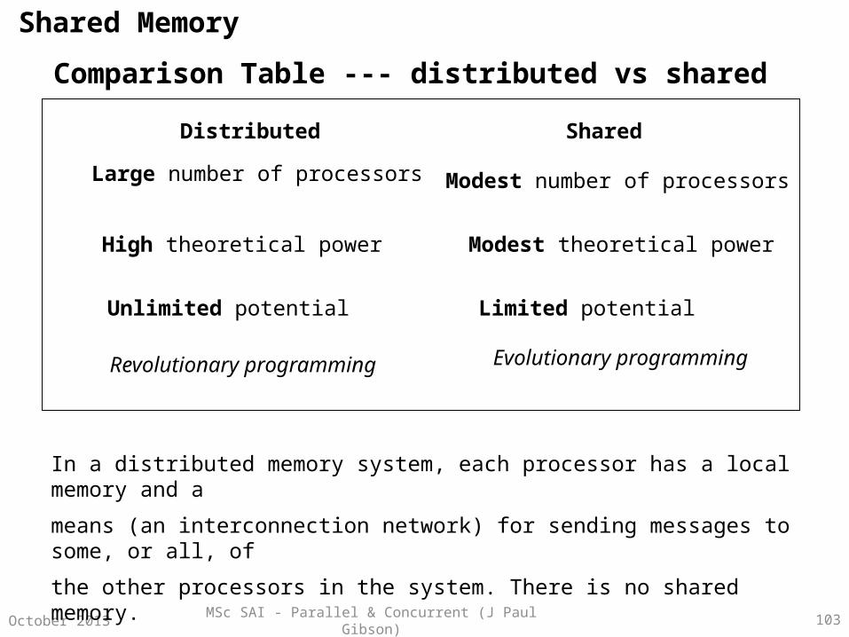
Comparison Table --- distributed vs shared
Distributed Shared
Large number of processors Modest number of processors
High theoretical power Modest theoretical power
Unlimited potential Limited potential
Revolutionary programming Evolutionary programming
In a distributed memory system, each processor has a local memory and a
means (an interconnection network) for sending messages to some, or all, of
the other processors in the system. There is no shared memory.
All synchronisation is done through message passing.
Shared Memory
MSc SAI - Parallel & Concurrent (J Paul Gibson) 104October 2013
Message passing
•With message passing, sometimes a lot of data needs to be sent from process to process. This may cause a lot of communication overhead and cost a lot of time.•With message passing, sometimes messages have to go through intermediate nodes.•With message passing we have to worry about synchronising transmission.•Sometimes, with message passing, processes have to wait for information from other processes before they can continue.•What happens if we have circular waits between processes --- deadlock … nothing can happen
But,it is a much more flexible and powerful means of utilising parallel processes…. Although, is it parallel processing?

MSc SAI - Parallel & Concurrent (J Paul Gibson) 105October 2013
Hybrid Architectures ---
mixing shared and distributed
A good example, often found in the real world, are clusters of processors, where a high speed bus serves for intra cluster communication, and an interconnection network is used for inter cluster communication.

MSc SAI - Parallel & Concurrent (J Paul Gibson) 106October 2013
•Shared memory ---???--- use mutual exclusion mechanism
•Distributed memory ---???--- use synchronisation mechanism
•Sequentially
sum := A[0]
For I := 1 to m-1
sum := sum+A[I]
To parallelise: if we have n processors then we can calculate the sum of m/nnumbers on each, and the sum of these partial sums gives the result … easy?
Example --- summing m numbers
NOTE: Comparative analysis between distributed, shared and hybrid architectures can be more difficult than this simple example.
Shared Memory vs Message Passing vs Hybrid
MSc SAI - Parallel & Concurrent (J Paul Gibson)October 2013 107
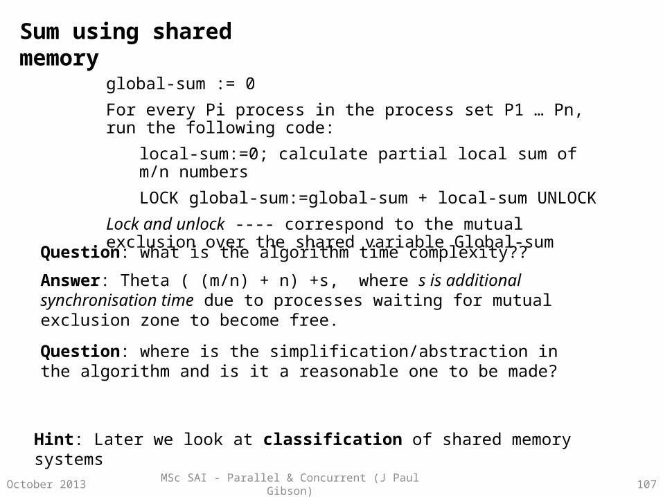
Sum using shared memory
global-sum := 0
For every Pi process in the process set P1 … Pn, run the following code:
local-sum:=0; calculate partial local sum of m/n numbers
LOCK global-sum:=global-sum + local-sum UNLOCK
Lock and unlock ---- correspond to the mutual exclusion over the shared variable Global-sum
Question: where is the simplification/abstraction in the algorithm and is it a reasonable one to be made?
Hint: Later we look at classification of shared memory systems
Question: what is the algorithm time complexity??
Answer: Theta ( (m/n) + n) +s, where s is additional synchronisation time due to processes waiting for mutual exclusion zone to become free.

MSc SAI - Parallel & Concurrent (J Paul Gibson) 108October 2013
Sum using distributed memory
We have to map onto a particular communication architecture to be able to control/program the synchronisation. For simplicity, we chose a 3*3 array of processors in a square mesh architecture:
P11
P21
P31
P12
P22
P32
P13
P23
P33
Algorithm --- each processor finds the sum of its m/n numbers. Then it passes this value to another processor which sums all its input (see the solid lines in the diagram), until finally P11 contains the result.
NOTE: we studied this – including complexity analysis - previously
MSc SAI - Parallel & Concurrent (J Paul Gibson) 109October 2013
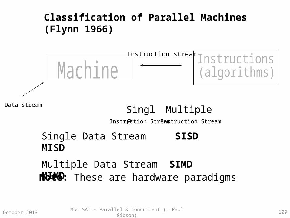
Classification of Parallel Machines (Flynn 1966)
Single Data Stream SISD MISD
Multiple Data Stream SIMD MIMD
Single
Note: These are hardware paradigms
Instruction Stream Instruction Stream
Multiple
Instruction stream
Data stream

MSc SAI - Parallel & Concurrent (J Paul Gibson) 110October 2013
SISD --- Standard Sequential Computer
Examples: •1 Sum n numbers a1…an -- n memory reads, n-1 additions => O(n)
•2 Sort n numbers a1… an -- O(??)
•3 Sort n numbers a1…an and m numbers b1…bm -- O(??)
Instructions
Data Stream

MSc SAI - Parallel & Concurrent (J Paul Gibson) 111October 2013
MISD (n processors)
Parallelism: Processors do different things at the same time on the same datum
Example: check if Z is prime, if n=Z-2 then what can we do?
Answer: Each Pm checks if m-2 divides evenly into Z
IS1
ISn
Single DS
MSc SAI - Parallel & Concurrent (J Paul Gibson) 112October 2013
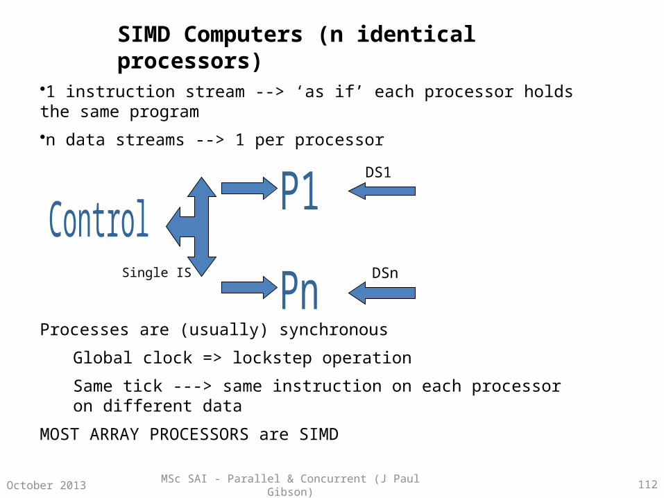
SIMD Computers (n identical processors)
•1 instruction stream --> ‘as if’ each processor holds the same program
•n data streams --> 1 per processor
Processes are (usually) synchronous
Global clock => lockstep operation
Same tick ---> same instruction on each processor on different data
MOST ARRAY PROCESSORS are SIMD
Single IS
DS1
DSn
MSc SAI - Parallel & Concurrent (J Paul Gibson) 113October 2013
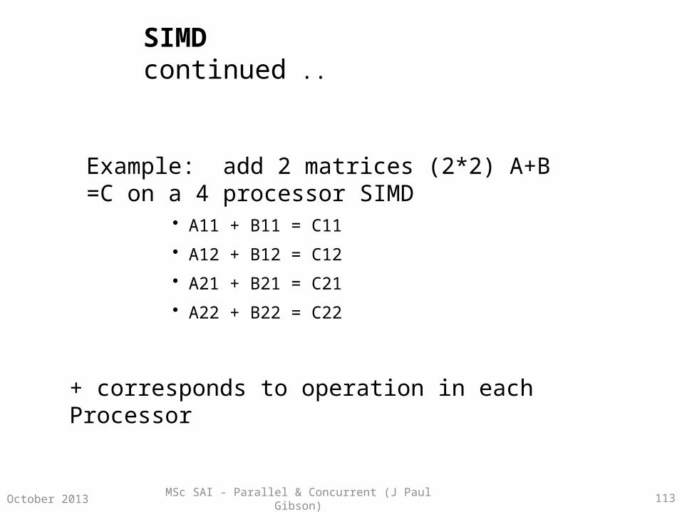
SIMD continued ..
Example: add 2 matrices (2*2) A+B =C on a 4 processor SIMD
• A11 + B11 = C11
• A12 + B12 = C12
• A21 + B21 = C21
• A22 + B22 = C22
+ corresponds to operation in each Processor
MSc SAI - Parallel & Concurrent (J Paul Gibson) 114October 2013
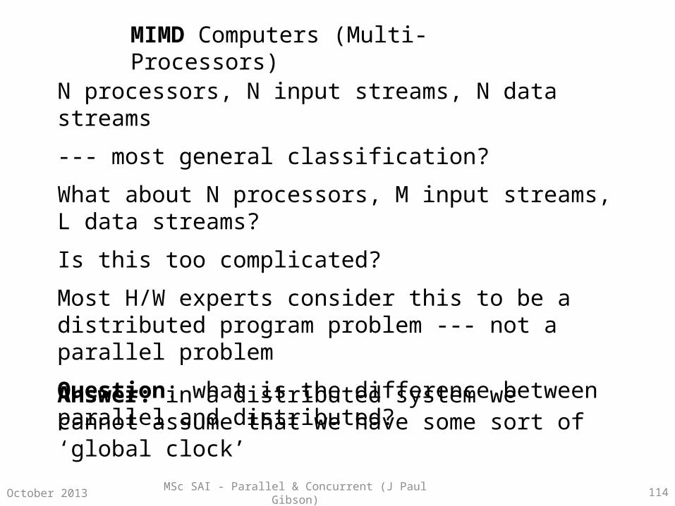
MIMD Computers (Multi-Processors)
N processors, N input streams, N data streams
--- most general classification?
What about N processors, M input streams, L data streams?
Is this too complicated?
Most H/W experts consider this to be a distributed program problem --- not a parallel problem
Question: what is the difference between parallel and distributed?
Answer: in a distributed system we cannot assume that we have some sort of ‘global clock’

MSc SAI - Parallel & Concurrent (J Paul Gibson) 115October 2013
MIMD continued
•Processes are typically asynchronous•MIMDs with shared memory are tightly coupled machines•MIMDs on an interconnection network are loosely coupled machines
IS1
ISn
DS1
DSn

MSc SAI - Parallel & Concurrent (J Paul Gibson) 116October 2013
MIMD continued ...
Architecture with most potential
Example: Calculate (A+B)-(C*D) for 2*2 matrices A,B,C and D
With the following number of processors:
3, 8, 12 and n.
Question: What about this 3 Processor Architecture?
A+B C*D ??

MSc SAI - Parallel & Concurrent (J Paul Gibson) 117October 2013
Shared memory computer classification
Depending on whether 2 or more processors are allowed to simultaneously read from or write to the same location simultaneously, we have 4 classes of shared memory computers:
•Exclusive Read, Exclusive Write (EREW) SM --- access to memory is exclusive, so that no two processors are allowed to simultaneously read or write to same location.
•Concurrent Read, Exclusive Write (CREW) --- multiple processors are allowed to read simultaneously.
•Exclusive Read, Concurrent Write (ERCW) --- read remain exclusive but writes can be concurrent
•Concurrent Read, Concurrent Write (CRCW) --- both reading and writing can be done simultaneously.
MSc SAI - Parallel & Concurrent (J Paul Gibson) 118October 2013
Write Conflicts in shared memory
If several processors are trying to simultaneously store (potentially different) data at the same address, which of them should succeed? … We need a deterministic way of specifying the contents of a memory location after a concurrent write:
• Assign priorities to the processors• All processors can write, provided they attempt to write the same thing, otherwise
all access is denied• The max/min/sum/average of the value is stored (for numeric data)• The closest/best result is stored (depending on problem to be solved)
But, it is only feasible (on a fast bus) for P processors to write simultaneously for small P (<30, eg). Usually the cost of communication hardware is too high.

MSc SAI - Parallel & Concurrent (J Paul Gibson) 119October 2013
Shared memory consequences
on multiple data machines
Generally, SIMD machines typically need a large number of processors.
Question: why??
Answer: because there is no control unit, and each of the processors is very simple
In MIMD machines, which use much more powerful processors, shared memory systems are found with small numbers of processors
MSc SAI - Parallel & Concurrent (J Paul Gibson) 120October 2013
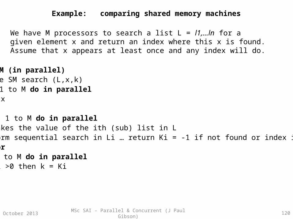
Example: comparing shared memory machines
We have M processors to search a list L = l1,…ln for a given element x and return an index where this x is found. Assume that x appears at least once and any index will do.
ALGORITHM (in parallel)Procedure SM search (L,x,k)For I = 1 to M do in parallel
read xEndfor
For I 1 to M do in parallelLi takes the value of the ith (sub) list in Lperform sequential search in Li … return Ki = -1 if not found or index if foundEndfor
For I =1 to M do in parallelif Ki >0 then k = Ki
Endfor

MSc SAI - Parallel & Concurrent (J Paul Gibson)October 2013 13.121
Comparing shared memory machines continued...
•EREW
•ERCW
•CREW
•CRCW
•O(M) for M reads •O(n/M) for reading list and sequential search•O(M) for M writes
•O(M)•O(n/M)•Constant time
•Constant time•O(n/M)•O(N) time
•Constant time•O(n/M) time•Constant time
Question: what are the time complexities of the algorithm on each of our 4 shared memory computers (EREW,ERCW,CREW,CRCW)??
MSc SAI - Parallel & Concurrent (J Paul Gibson) 122October 2013
Parallel Architectures – Further Reading
Michael J. Flynn. 1972. Some computer organizations and their effectiveness. IEEE Trans. Comput. 21, 9 (September 1972), 948-960
Ralph Duncan. 1990. A Survey of Parallel Computer Architectures. Computer 23, 2 (February 1990), 5-16.
John M. Mellor-Crummey and Michael L. Scott. 1991. Algorithms for scalable synchronization on shared-memory multiprocessors. ACM Trans. Comput. Syst. 9, 1 (February 1991), 21-65.
MSc SAI - Parallel & Concurrent (J Paul Gibson) 123October 2013
An Introduction to MPI
• Message Passing Interface (MPI)• Computation is made of:
– One or more processes– Communicate by calling
library routines• MIMD programming model• SPMD most common.

MSc SAI - Parallel & Concurrent (J Paul Gibson) 124October 2013
An Introduction to MPI
•Processes use point-to-point communication operations•Collective communication operations are also available.•Communication can be modularized by the use of communicators.
MPI_COMM_WORLD is the base. Used to identify subsets of processors

MSc SAI - Parallel & Concurrent (J Paul Gibson) 125October 2013
An Introduction to MPI
•Complex, but most problems can be solved using the 6 basic functions.
MPI_Init MPI_Finalize MPI_Comm_size MPI_Comm_rank MPI_Send MPI_Recv

MSc SAI - Parallel & Concurrent (J Paul Gibson) 126October 2013
An Introduction to MPI
Most calls require a communicator handle as an argument.
MPI_COMM_WORLD
MPI_Init and MPI_Finalize don’t require a communicator handle used to begin and end an MPI program MUST be called to begin and end

MSc SAI - Parallel & Concurrent (J Paul Gibson) 127October 2013
An Introduction to MPI
MPI_Comm_size determines the number of processors
in the communicator group
MPI_Comm_rank determines the integer identifier
assigned to the current process

MSc SAI - Parallel & Concurrent (J Paul Gibson) 128October 2013
An Introduction to MPI
// MPI1.cc#include "mpi.h"#include <stdio.h>
int main( argc, argv )int argc;char **argv;{
MPI_Init( &argc, &argv );printf( "Hello world\n" );MPI_Finalize();return 0;
}

MSc SAI - Parallel & Concurrent (J Paul Gibson) 129October 2013
An Introduction to MPI
// MPI2.cc#include <stdio.h>#include <mpi.h>
main(int argc, char *argv[]){
int iproc, nproc;MPI_Init(&argc, &argv);MPI_Comm_size(MPI_COMM_WORLD, &nproc);MPI_Comm_rank(MPI_COMM_WORLD, &iproc);printf("I am processor %d of %d\n", iproc, nproc);MPI_Finalize();
}
MSc SAI - Parallel & Concurrent (J Paul Gibson) 130October 2013
An Introduction to MPI
MPI Communication
• MPI_Send– Sends an array of a given type– Requires a destination node, size, and type
• MPI_Recv– Receives an array of a given type– Same requirements as MPI_Send– Extra parameter
• MPI_Status variable.
MSc SAI - Parallel & Concurrent (J Paul Gibson) 131October 2013
An Introduction to MPI
• Made originally for both FORTRAN and C (and C++)• Standards for C
– MPI_ prefix to all calls– First letter of function name is capitalized– Returns MPI_SUCCESS or error code– MPI_Status structure– MPI data types for each C type
There is also mpiJava: http://www.hpjava.org/mpiJava.html
Also take a look at Open MPI http://www.open-mpi.org/

MSc SAI - Parallel & Concurrent (J Paul Gibson) 132October 2013
An Introduction to MPI
• Message Passing programs are non-deterministic because of concurrency– Consider 2 processes sending messages to third
• MPI does guarantee that 2 messages sent from a single process to another will arrive in order.
• It is the programmer's responsibility to ensure computation determinism

MSc SAI - Parallel & Concurrent (J Paul Gibson) 133October 2013
An Introduction to MPI
• MPI & Determinism – A Process may specify the source of the message– A Process may specify the type of message
• Non-Determinism– MPI_ANY_SOURCE or MPI_ANY_TAG
MSc SAI - Parallel & Concurrent (J Paul Gibson) 134October 2013
An Introduction to MPI
Global Operations
• Coordinated communication involving multiple processes.• Can be implemented by the programmer using sends and
receives• For convenience, MPI provides a suite of collective
communication functions.

MSc SAI - Parallel & Concurrent (J Paul Gibson) 135October 2013
An Introduction to MPI
Collective Communication
• Barrier– Synchronize all processes
• Broadcast• Gather
– Gather data from all processes to one process• Scatter• Reduction
– Global sums, products, etc.

MSc SAI - Parallel & Concurrent (J Paul Gibson) 136October 2013
An Introduction to MPI
MSc SAI - Parallel & Concurrent (J Paul Gibson) 137October 2013
An Introduction to MPI
Other MPI Features
• Asynchronous Communication– MPI_ISend– MPI_Wait and MPI_Test– MPI_Probe and MPI_Get_count
• Modularity– Communicator creation routines
• Derived Datatypes
MSc SAI - Parallel & Concurrent (J Paul Gibson) 138October 2013
An Introduction to MPI
Getting to compile, execute and profile/analyse programs using MPI on any ‘parallel’ computer seems to require a very steep learning curve:
• Non-standard installs
• Architecture issues
• OS issues
• Support issues
NOTE: There are alternatives like PVM - http://www.csm.ornl.gov/pvm/
MSc SAI - Parallel & Concurrent (J Paul Gibson) 139October 2013
How to Use MPI on a Unix cluster
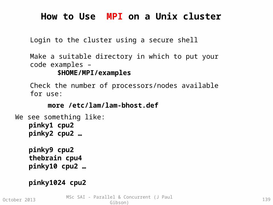
Login to the cluster using a secure shell
Make a suitable directory in which to put your code examples –$HOME/MPI/examples
Check the number of processors/nodes available for use:
more /etc/lam/lam-bhost.def
We see something like:pinky1 cpu2pinky2 cpu2 …
pinky9 cpu2thebrain cpu4pinky10 cpu2 …
pinky1024 cpu2
MSc SAI - Parallel & Concurrent (J Paul Gibson) 140October 2013
How to Use MPI on our cluster
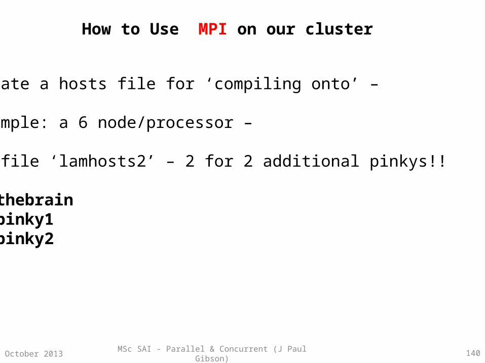
Create a hosts file for ‘compiling onto’ –
Example: a 6 node/processor –
In file ‘lamhosts2’ – 2 for 2 additional pinkys!!
thebrainpinky1pinky2

MSc SAI - Parallel & Concurrent (J Paul Gibson)October 2013 9.141
How to Use MPI on our cluster
$ recon -v lamhosts2
recon: -- testing n0 (thebrain)
recon: -- testing n1 (pinky1)
pgibson@pinky1's password:
recon: -- testing n2 (pinky2)
pgibson@pinky2's password:
$
--------------------------------------------------Woo hoo!
recon has completed successfully. This means that you will most likelybe able to boot LAM successfully with the lamboot" command (but this is not a guarantee). See the lamboot(1) manual page for more Information on the lamboot command….
Use the recon tool to verify that the cluster is bootable:

MSc SAI - Parallel & Concurrent (J Paul Gibson) 142October 2013
How to Use MPI on our cluster
Use the lamboot tool to start LAM on the specified cluster$ lamboot -v lamhosts2
LAM (Local Area Multicomputer) is an MPI programming environment and development system for heterogeneous computers on a network. With LAM, a dedicated cluster or an existing network computing infrastructure can act as one parallel computer solving one problem.
LAM features extensive debugging support in the application development cycle and peak performance for production applications. LAM features a full implementation of the MPI communication standard.
Executing hboot on n0 (thebrain - 1 CPU)...Executing hboot on n1 (pinky1 - 1 CPU)...pgibson@pinky1's password: pgibson@pinky1's password: Executing hboot on n2 (pinky2 - 1 CPU)...pgibson@pinky2's password: pgibson@pinky2's password: topology done

MSc SAI - Parallel & Concurrent (J Paul Gibson) 143October 2013
How to Use MPI on a cluster
// MPI1.cc#include "mpi.h“// or include <mpi.h>
#include <stdio.h>
int main( int argc, char** argv )
{MPI_Init( &argc, &argv );printf( "Hello world\n" );MPI_Finalize();return 0;}
Compiling and running MPI1.cc
$ mpicc -o mpi1 mpi1.cc
$ lslamhosts2 mpi1 mpi1.cc
$ mpirun -v -np 1 mpi1
343 mpi1 running on n0 (o)Hello world

MSc SAI - Parallel & Concurrent (J Paul Gibson) 144October 2013
How to Use MPI on a clusterCompiling and running the same code on multiple ‘processors’:
$mpirun –v –np 10 mpi1395 mpi1 running on n0 (o)10659 mpi1 running on n110908 mpi1 running on n2396 mpi1 running on n0 (o)10660 mpi1 running on n110909 mpi1 running on n2397 mpi1 running on n0 (o)10661 mpi1 running on n110910 mpi1 running on n2398 mpi1 running on n0 (o)Hello worldHello worldHello worldHello worldHello worldHello worldHello worldHello worldHello worldHello world

MSc SAI - Parallel & Concurrent (J Paul Gibson) 145October 2013
How to Use MPI on a cluster
OTHER IMPORTANT TOOLS –
mpitask - for monitoring mpi applications
lamclean – for cleaning LAM
lamhalt – for terminating LAM
wipe – when lamhalt hangs and you need to pull the plug!!

MSc SAI - Parallel & Concurrent (J Paul Gibson) 146October 2013
How to Use MPI on a cluster
#include <stdio.h>
#include <mpi.h>
main(int argc, char *argv[])
{
int iproc, nproc;
MPI_Init(&argc, &argv);
MPI_Comm_size(MPI_COMM_WORLD, &nproc);
MPI_Comm_rank(MPI_COMM_WORLD, &iproc);
printf("I am processor %d of %d\n", iproc, nproc);
MPI_Finalize();
}
How do we run this on a number of different processors?

MSc SAI - Parallel & Concurrent (J Paul Gibson) 147October 2013
How to Use MPI on the cluster
[pgibson@TheBrain examples]$ mpirun -np 1 mpi2I am processor 0 of 1[pgibson@TheBrain examples]$ mpirun -np 2 mpi2I am processor 0 of 2I am processor 1 of 2[pgibson@TheBrain examples]$ mpirun -np 3 mpi2I am processor 0 of 3I am processor 1 of 3I am processor 2 of 3[pgibson@TheBrain examples]$ mpirun -np 4 mpi2I am processor 0 of 4I am processor 3 of 4I am processor 1 of 4I am processor 2 of 4

MSc SAI - Parallel & Concurrent (J Paul Gibson) 148October 2013
How to Use MPI on the cluster
[pgibson@TheBrain examples]$ mpirun -np 20 mpi2I am processor 0 of 20I am processor 6 of 20I am processor 12 of 20I am processor 9 of 20I am processor 3 of 20I am processor 15 of 20I am processor 18 of 20I am processor 1 of 20I am processor 4 of 20I am processor 2 of 20I am processor 16 of 20I am processor 5 of 20I am processor 8 of 20I am processor 13 of 20I am processor 10 of 20I am processor 7 of 20I am processor 19 of 20I am processor 14 of 20I am processor 17 of 20I am processor 11 of 20

MSc SAI - Parallel & Concurrent (J Paul Gibson) 149October 2013
MPI – further reading
William Gropp, Ewing Lusk, Nathan Doss, and Anthony Skjellum. 1996. A high-performance, portable implementation of the MPI message passing interface standard. Parallel Comput. 22, 6 (September 1996), 789-828.
Edgar Gabriel and Graham E. Fagg and George Bosilca and Thara Angskun and Jack Dongarra and Jeffrey M. Squyres and Vishal Sahay and Prabhanjan Kambadur and Brian Barrett and Andrew Lumsdaine and Ralph H. Castain and David J. Daniel and Richard L. Graham and Timothy S. Woodall , Open MPI: Goals, Concept, and Design of a Next Generation MPI Implementation. In Recent Advances in Parallel Virtual Machine and Message Passing Interface, 11th European PVM/MPI Users' Group Meeting, Budapest, Hungary, September 19-22, 2004, Proceedings PVM/MPI 2004
MSc SAI - Parallel & Concurrent (J Paul Gibson) 150October 2013
Sequential to parallel ---specification to implementation
Often a piece of sequential code defines the functional requirements of a system
However, these functional requirements do not address resource issues:• speed requirements• space requirements• cost requirements• efficiency requirements, etc …
A lot of work may have gone into proving the functional requirements correct ---• validation• verification
How can we re-use this work when developing a system which meets the functional
and non-functional needs?
We transform the sequential code to make it parallel. This parallel code can• automatically meet functional requirements if the transformation is correct• be shown to meet the non-functional requirements using analysis techniques
MSc SAI - Parallel & Concurrent (J Paul Gibson) 151October 2013
Sequential to parallel ---
specification to implementation
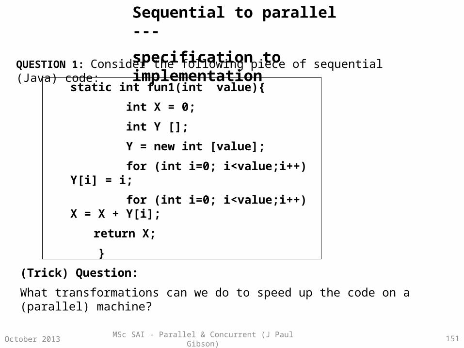
static int fun1(int value){
int X = 0;
int Y [];
Y = new int [value];
for (int i=0; i<value;i++) Y[i] = i;
for (int i=0; i<value;i++) X = X + Y[i];
return X;
}
QUESTION 1: Consider the following piece of sequential (Java) code:
(Trick) Question:
What transformations can we do to speed up the code on a (parallel) machine?

MSc SAI - Parallel & Concurrent (J Paul Gibson) 152October 2013
static int fun1(int value){
int X = 0;
int Y [];
Y = new int [value];
for (int i=0; i<value;i++) Y[i] = i;
for (int i=0; i<value;i++) X = X + Y[i];
return X;
}
Need to first ask – what is it doing … ?
class example1 {
public static void main(String [] args){ for (int i=0; i< 6;i++) System.out.println("fun1("+i+") = " + fun1(i) ); }
Write some test code !!fun1(0) = 0
fun1(1) = 0fun1(2) = 1fun1(3) = 3fun1(4) = 6fun1(5) = 10
And examine output
Sequential to parallel

MSc SAI - Parallel & Concurrent (J Paul Gibson)October 2013 12.153
static int fun1(int value){
// int X = 0;
//int Y [];
//Y = new int [value];
// for (int i=0; i<value;i++) Y[i] = i;
//for (int i=0; i<value;i++) X = X + i;
return (value*(value-1)/2);
}
Need to then ask – how is it doing it … ‘foolishly’?
class example1 {
public static void main(String [] args){ for (int i=0; i< 6;i++) System.out.println("fun1("+i+") = " + fun1(i) ); }
Transformoriginal function
fun1(0) = 0fun1(1) = 0fun1(2) = 1fun1(3) = 3fun1(4) = 6fun1(5) = 10
And examine output
Sequential to parallel

MSc SAI - Parallel & Concurrent (J Paul Gibson) 154October 2013
static int fun1(int value){
int X = 0;
int Y [];
Y = new int [value];
// for (int i=0; i<value;i++) Y[i] = i;
for (int i=0; i<value;i++) X = X + i;
return X;
}
Need to then ask – how is it doing it… ?
class example1 {
public static void main(String [] args){ for (int i=0; i< 6;i++) System.out.println("fun1("+i+") = " + fun1(i) ); }
Transformoriginal function
fun1(0) = 0fun1(1) = 0fun1(2) = 1fun1(3) = 3fun1(4) = 6fun1(5) = 10
And examine output
Sequential to parallel
MSc SAI - Parallel & Concurrent (J Paul Gibson) 155October 2013
Lessons to learn
• Sometimes ‘transforming out’ the poor sequential code – without thinking about a parallel implementation – is all that is required to improve performance
•Do not underestimate the poor quality of the original code
•Be careful not to change the behaviour
•Reason in small (incremental) steps that functional behaviour is maintained
•Sometimes simple mathematical analysis is enough – in example1 a simple proof by induction
•Sometimes testing is easier than a fully formal proof … but beware that testing is usually incomplete.
Sequential to parallel
MSc SAI - Parallel & Concurrent (J Paul Gibson) 156October 2013
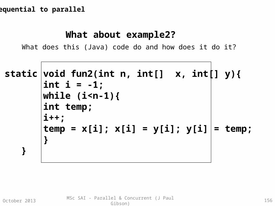
What about example2?
static void fun2(int n, int[] x, int[] y){ int i = -1; while (i<n-1){ int temp; i++; temp = x[i]; x[i] = y[i]; y[i] = temp; } }
What does this (Java) code do and how does it do it?
Sequential to parallel
MSc SAI - Parallel & Concurrent (J Paul Gibson) 157October 2013
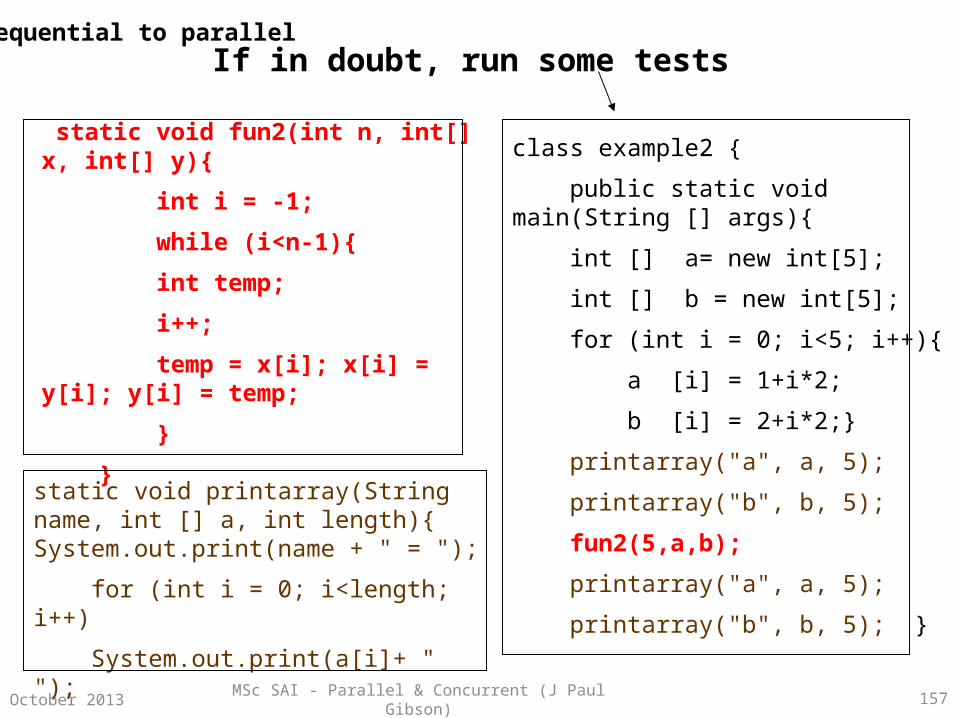
static void fun2(int n, int[] x, int[] y){
int i = -1;
while (i<n-1){
int temp;
i++;
temp = x[i]; x[i] = y[i]; y[i] = temp;
}
}
If in doubt, run some tests
class example2 {
public static void main(String [] args){
int [] a= new int[5];
int [] b = new int[5];
for (int i = 0; i<5; i++){
a [i] = 1+i*2;
b [i] = 2+i*2;}
printarray("a", a, 5);
printarray("b", b, 5);
fun2(5,a,b);
printarray("a", a, 5);
printarray("b", b, 5); }
static void printarray(String name, int [] a, int length){ System.out.print(name + " = ");
for (int i = 0; i<length; i++)
System.out.print(a[i]+ " ");
System.out.println();};
Sequential to parallel

MSc SAI - Parallel & Concurrent (J Paul Gibson) 158October 2013
Examine/Analyse results of test(s)
a = 1 3 5 7 9b = 2 4 6 8 10a = 2 4 6 8 10b = 1 3 5 7 9
Attempt to find/ reverse engineer a statement of the functional behaviour –
It appears to swap elements between arrays
Verify model by running more tests and/or formal reasoning …
Transform code to make it more efficient: 1) Change the data structure to ‘pointers’ and swapping whole array means just swapping 2 pointers!, or2) Identify that swaps can be done in parallel (any arbitrary interleaving is correct!)
Sequential to parallel
MSc SAI - Parallel & Concurrent (J Paul Gibson) 159October 2013
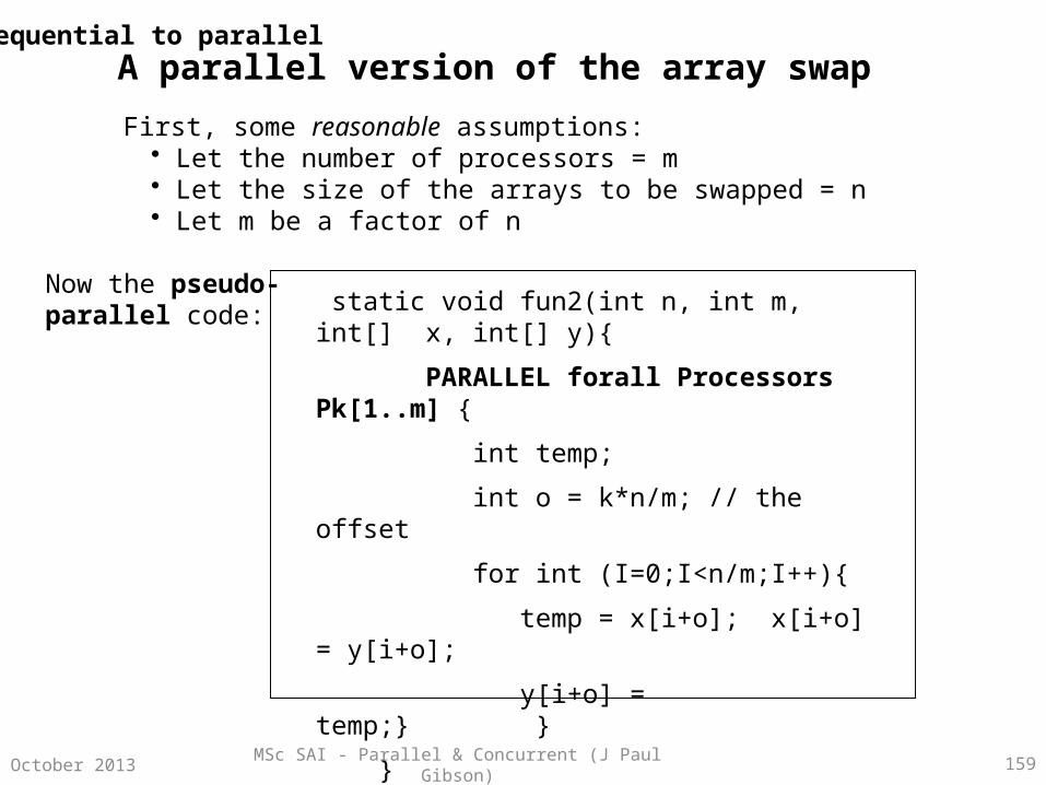
A parallel version of the array swap
First, some reasonable assumptions:• Let the number of processors = m• Let the size of the arrays to be swapped = n• Let m be a factor of n
Now the pseudo-parallel code: static void fun2(int n, int m, int[] x, int[] y){
PARALLEL forall Processors Pk[1..m] {
int temp;
int o = k*n/m; // the offset
for int (I=0;I<n/m;I++){
temp = x[i+o]; x[i+o] = y[i+o];
y[i+o] = temp;} }
}
Sequential to parallel
MSc SAI - Parallel & Concurrent (J Paul Gibson) 160October 2013
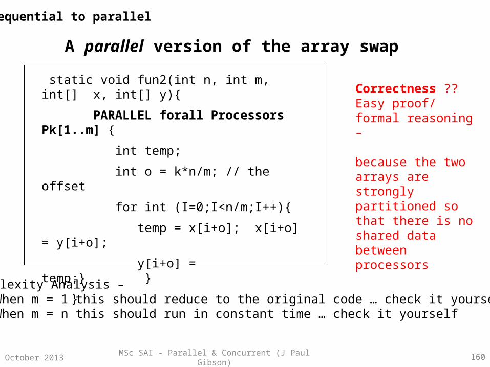
A parallel version of the array swap
static void fun2(int n, int m, int[] x, int[] y){
PARALLEL forall Processors Pk[1..m] {
int temp;
int o = k*n/m; // the offset
for int (I=0;I<n/m;I++){
temp = x[i+o]; x[i+o] = y[i+o];
y[i+o] = temp;} }
}
Complexity Analysis –1) When m = 1 this should reduce to the original code … check it yourself2) When m = n this should run in constant time … check it yourself
Correctness ??Easy proof/ formal reasoning –
because the two arrays are strongly partitioned so that there is no shared data between processors
Sequential to parallel

MSc SAI - Parallel & Concurrent (J Paul Gibson) 161October 2013
What about example3?
What does this (Java) code do and how does it do it?
static int fun3(int n, int [] X){ int sum, mid; sum = 0; for (int i = 0; i<n; i++) sum = X[i]+sum; mid = sum/2; sum = 0; int i =0; do{sum = sum+X[i];i++; } while (sum<mid); return i; }
Sequential to parallel

MSc SAI - Parallel & Concurrent (J Paul Gibson) 162October 2013
If in doubt, run some tests
class example3 {
public static void main(String [] args){
int [] a= new int[15];
int [] b = new int[15];
for (int i = 0; i<15; i++){
a [i] = 10/(i+1);
b [i] = i*i*i;}
printarray("a", a, 15); \\ see defn before
System.out.println( fun3(15,a) );
printarray("b", b, 15); \\ see defn before
System.out.println( fun3(15,b) );
}
QUESTION: What is the output?
Can youreverse engineer a statement of the functional behaviour?
Sequential to parallel
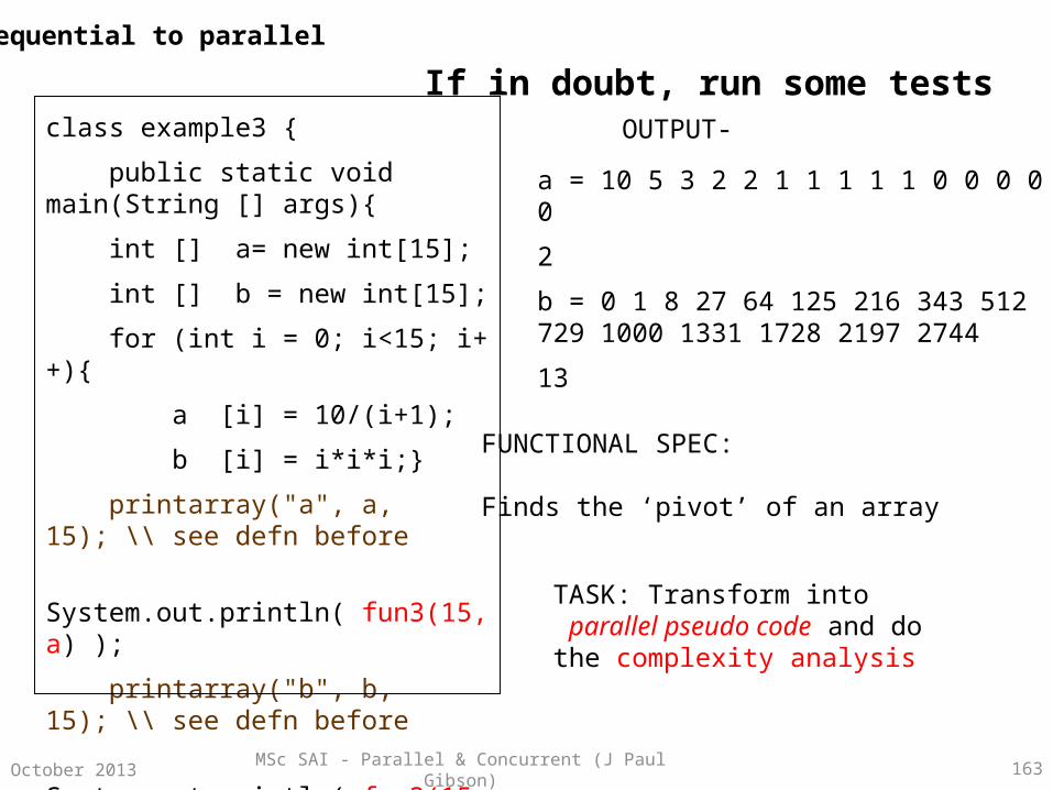
MSc SAI - Parallel & Concurrent (J Paul Gibson) 163October 2013
If in doubt, run some testsclass example3 {
public static void main(String [] args){
int [] a= new int[15];
int [] b = new int[15];
for (int i = 0; i<15; i++){
a [i] = 10/(i+1);
b [i] = i*i*i;}
printarray("a", a, 15); \\ see defn before
System.out.println( fun3(15,a) );
printarray("b", b, 15); \\ see defn before
System.out.println( fun3(15,b) );
}
a = 10 5 3 2 2 1 1 1 1 1 0 0 0 0 0
2
b = 0 1 8 27 64 125 216 343 512 729 1000 1331 1728 2197 2744
13
OUTPUT-
FUNCTIONAL SPEC:
Finds the ‘pivot’ of an array
TASK: Transform into parallel pseudo code and do the complexity analysis
Sequential to parallel
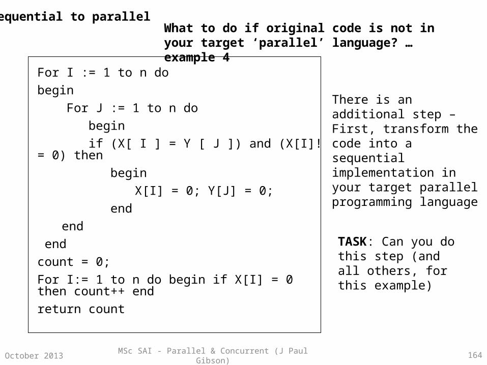
MSc SAI - Parallel & Concurrent (J Paul Gibson) 164October 2013
For I := 1 to n dobegin For J := 1 to n do begin if (X[ I ] = Y [ J ]) and (X[I]!= 0) then
beginX[I] = 0; Y[J] = 0;
endend
endcount = 0;For I:= 1 to n do begin if X[I] = 0 then count++ endreturn count
What to do if original code is not in your target ‘parallel’ language? … example 4
There is an additional step –First, transform the code into a sequential implementation in your target parallel programming language
TASK: Can you do this step (and all others, for this example)
Sequential to parallel

MSc SAI - Parallel & Concurrent (J Paul Gibson) 165October 2013
QUESTION 5: A classic parallelisation example
For I := 1 to n do
begin
temp := X[ I ]
X[ I ] := X [ n+1- I ]; X [n+1 - I ] := temp
end
Sequential to parallel

MSc SAI - Parallel & Concurrent (J Paul Gibson) 166October 2013
QUESTION 6: A more difficult classic parallelisation example
Int big = X[1];Int smallest = Y[1];For j := 1 to n dobeginFor I := j to n dobegin if X[I] > big then begin big = X[I]; swap (X[j], X[I]) end if Y[I] < smallest then begin smallest = Y[I]; swap (Y[j], Y[I]) endendX[j] = biggest+smallestend

MSc SAI - Parallel & Concurrent (J Paul Gibson) 167October 2013
Mathematical Models for Analysing Parallel Systems
A parallel algorithm is an algorithm for the execution of a program which involves the running of two or more processes on two or more processors simultaneously.
Two important measures of the quality of parallelism are:
• speedup, and
• efficiency
If Ts is the time taken to run the fastest serial algorithm on one process and if Tp is the time taken by the parallel algorithm on N processors then:
Speedup = S(N) = Ts/Tp, and
Efficiency = E(N) = S(N)/N
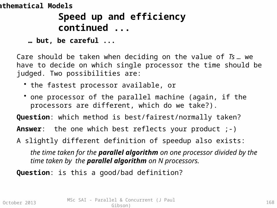
MSc SAI - Parallel & Concurrent (J Paul Gibson) 168October 2013
Speed up and efficiency continued ...
Care should be taken when deciding on the value of Ts … we have to decide on which single processor the time should be judged. Two possibilities are:
• the fastest processor available, or
• one processor of the parallel machine (again, if the processors are different, which do we take?).
Question: which method is best/fairest/normally taken?
Answer: the one which best reflects your product ;-)
A slightly different definition of speedup also exists:
the time taken for the parallel algorithm on one processor divided by the time taken by the parallel algorithm on N processors.
Question: is this a good/bad definition?
… but, be careful ...
Mathematical Models

MSc SAI - Parallel & Concurrent (J Paul Gibson) 169October 2013
Fibonacci 0.90 1.35 1.35 1.35 1.35Pyramid 0.90 1.32 1.30 1.30 1.30Mat Mult 1.21 1.76 1.80 1.77 1.62Dual Dag 1.94 1.65 1.45 1.45 1.45Whetstone 1.37 1.40 1.67 1.47 1.47FFT 1.69 2.56 2.52 2.55 2.55
We are going to see that throwing more and more processors at a problem does not always yield more and more speed-up.
Today, we will look at the formal reasoning which explains why …
Speed-up has its limits!
PREVIOUS LIMIT EXAMPLES FROM REAL DATA ANALYSIS
Mathematical Models

MSc SAI - Parallel & Concurrent (J Paul Gibson) 170October 2013
Factors that limit speedup
The ideal is to produce linear speedup, i.e produce a speedup of N using N processors, and thus have an efficiency of 1 (100%).However, in practice the speedup is reduced from its ideal because of:•Software Overhead --- Even with a completely equivalent algorithm, software overhead arises in the concurrent implementation (e.g. an additional index calculation required for splitting up data). In general, the parallel code will contain more lines of code!•Load Balancing ---Speedup is generally limited by the speed of the slowest node. Thus we try to ensure that each node performs the same amount of work, i.e. is load balanced.•Communication Overhead ---Assuming that communication and calculation cannot be overlapped, then any time spent communicating the data between processors directly degrades the speedup. Goal --- make the grain size (relative amount of work done between synchronisation-communication) as large as possible, whilst keeping the processors busy.
Mathematical Models

MSc SAI - Parallel & Concurrent (J Paul Gibson) 171October 2013
Amdahl’s Law
The speedup of a parallel algorithm is effectively limited by the number of operations which must be performed sequentially, i.e. its Serial Fraction
Let
S be the amount of time spent (by 1 processor) on serial parts of the program, and
P be the amount of time spent (by 1 processor) on parts that could be done in parallel.
Then:
Tseq = S+P, and
Tpar = S + P/N, where N = number of processors.
Thus, speedup = Tseq/Tpar
= (S+P) / (S+P/N)
Mathematical Models

MSc SAI - Parallel & Concurrent (J Paul Gibson) 172October 2013
Amdahl’s Law continued...
Example:
A program with 100 operations, each taking 1 time unit.
80 operations in parallel => P =80
20 operations in sequence => S = 20
Then, using 80 processors, we have:
Speedup = 100/(20+80/80) = 100/21 <5
Thus, a speedup of only 5 is possible no matter how many processors N !!
Mathematical Models
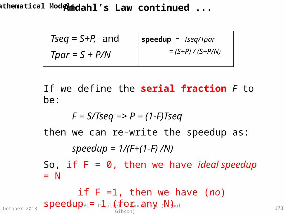
MSc SAI - Parallel & Concurrent (J Paul Gibson) 173October 2013
Amdahl’s Law continued ...
If we define the serial fraction F to be:
F = S/Tseq => P = (1-F)Tseq
then we can re-write the speedup as:
speedup = 1/(F+(1-F) /N)
So, if F = 0, then we have ideal speedup = N
if F =1, then we have (no) speedup = 1 (for any N)
Tseq = S+P, and
Tpar = S + P/N
speedup = Tseq/Tpar
= (S+P) / (S+P/N)
Mathematical Models
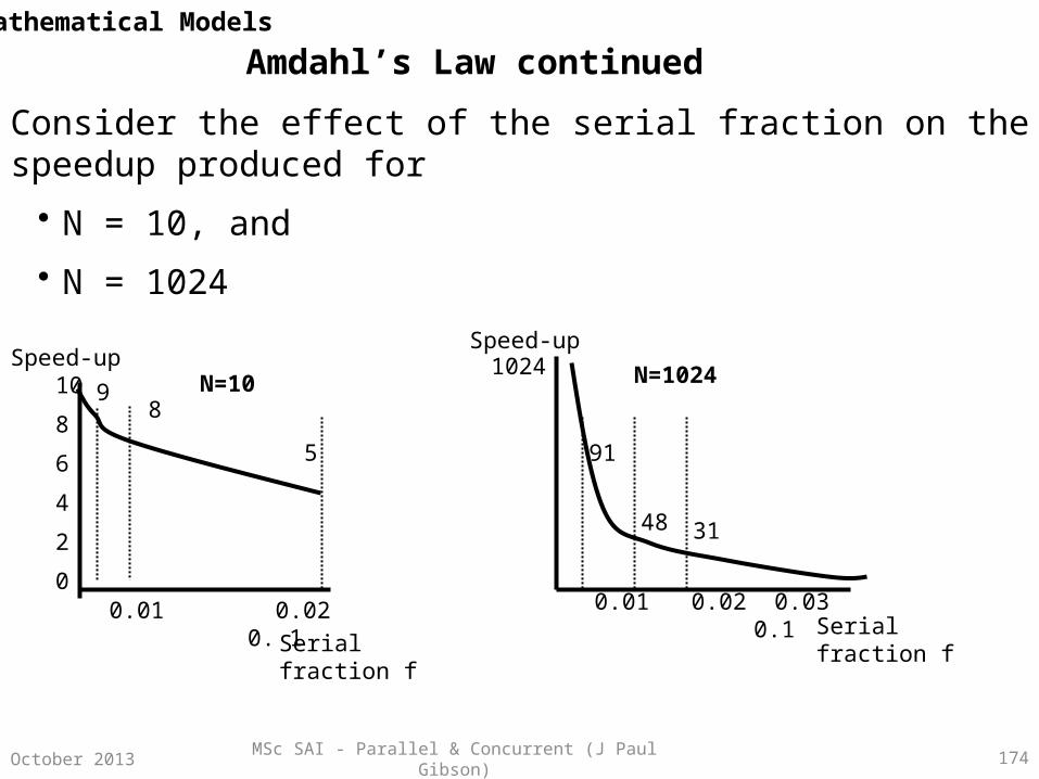
MSc SAI - Parallel & Concurrent (J Paul Gibson) 174October 2013
Amdahl’s Law continued
Consider the effect of the serial fraction on the speedup produced for
• N = 10, and
• N = 1024
0.01 0.02 0. 1Serial fraction f
Serial fraction f 0.01 0.02 0.03 0.1
10
8
6
4
2
0
1024
5
89 N=10 N=1024
91
48 31
Speed-upSpeed-up
Mathematical Models

MSc SAI - Parallel & Concurrent (J Paul Gibson) 175October 2013
Amdahl’s Law continued…
Amdahl’s law tells us that the serial fraction F places a severe constraint on the speedup as the number of processors increase.
Since most parallel programs contain a certain amount of sequential code, a possible conclusion of Amdahl’s Law is that it is not cost effective to build systems with large numbers of processors
However, most of the important applications that need to be parallelised contain very small fractions (<0.001)
From the graphs on the previous slide we see that:
• If 1% of a parallel program involves serial code, the maximum speedup that can be obtained is 9 using 10 processors, but only 91 using 1024 processors.
Mathematical Models

MSc SAI - Parallel & Concurrent (J Paul Gibson) 176October 2013
Using the serial fraction to measure performanceGiven the idealised serial fraction f, and N processors, we can calculate predicted speedup
speedup = 1/f +(1-f)/N
So, if we run the program and find the actual speedup,
Speedup =(Tseq/Tpar), then we can calculate
the actual serial fraction:
F = (1/Speedup -1/N)/ (1-1/N)
This F value is useful because it is not idealised. The idealised f assumes that all processors
compute for the same amount of time (i.e. are perfectly load balanced). Furthermore, the
idealised value does ignores communication and synchronisation overheads.
Note: load balancing effects are likely to result in irregular changes in F as N increases.
Mathematical Models
MSc SAI - Parallel & Concurrent (J Paul Gibson) 177October 2013
Measuring Performance (Example)
Say we have 12 tasks each requiring the same time. We have perfect load balancing for N = 2,3,4,6 and 12; but not for N = 5,7,8,9,10,11
Since a larger load imbalance results in a larger F, problems can be identified not apparent from speedup or efficiency.
Communication and synchronisation overhead tends to increase as N increases
Since increased overhead => decreased speedup, the value of F increases smoothly as N increases.
Note: a smoothly increasing F is a warning that grain size is too small. … think about this … we will come back to it!!
Mathematical Models

MSc SAI - Parallel & Concurrent (J Paul Gibson) 178October 2013
Measuring Performance (Example)
N Speed-Up EfficiencyF2 1.95 97 0.0243 2.88 96 0.0214 3.76 94 0.0218 6.96 87 0.021
Without looking at the serial fraction we cannot tell if the results are good. For example,why does the efficiency decrease? Since F is almost constant, we can conclude it is due to limited parallelism of the program.
Consider the following table of measurements:
Mathematical Models

MSc SAI - Parallel & Concurrent (J Paul Gibson) 179October 2013
Grain Size and Speedup (Example)
Consider adding m numbers using N processors. Processors 1…N-1 compute the partial sum of m/N-1 numbers. These are passed on to processor Pn to calculate the final sum.
P1 P2 Pn-1
Pn
There are N-1 communications
Each + takes 1 unit
100 units to pass partial sums
Assumptions
Question: what is speed-up (in terms of m and N)?
Mathematical Models

MSc SAI - Parallel & Concurrent (J Paul Gibson) 180October 2013
Grain Size and Speedup (Example)
P1 P2 Pn-1
Pn
There are N-1 communications
Each + takes 1 unit
100 units to pass partial sums
Assumptions
Parallel time = (M/(N-1))+(100)+(N-1)
We re-write as TP = (M+N*N+98N-99)/(N-1)
Sequential time TS = m ; thus speedup = Ts/Tp …=
(MN-M)/(M+N^2+98N-99)
Consider now the grain size … the amount of work done in each processor between synchronisations, in this case the size of M.
Question: what happens if M = 1000?
Mathematical Models

MSc SAI - Parallel & Concurrent (J Paul Gibson) 181October 2013
Grain Size and Speedup (Example) continued ...If M = 1000 and we use 10 processors thenspeedup = (10,000-1000)/(1000+100+980-99) =… = 4.54, andefficiency = 4.54 /10 = 45%
If m =10,000 and we use 10 processors thenspeedup = …. = 8.20efficiency = 82%
Thus, increasing grain size increases speedup and improves efficiency
Question: how would we take into account that some machines are better at calculating whilst others are better at data transfer?Answer: use the machine dependent ratio in our analysis
Mathematical Models

MSc SAI - Parallel & Concurrent (J Paul Gibson) 182October 2013
Using the machine dependent ratio
The machine dependent ratio is defined as Tcomm/Tcalc, where:
• Tcomm is the time to transfer a single word between nodes, and
• Tcalc is the time to perform some floating point calculation.
We can now generalise the example to obtain:
Tp = ((m/N-1)+N-1)Tcalc + Tcomm
Ts = m Tcalc
We can re-arrange to calculate the grain size required (size of m) for different machines (with different machine dependent ratios) in order to meet a certain level of efficiency.
For example, we require 80% efficiency (at least) on
• machine A with md ratio = 1 --- thus we need m>720
• machine B with md ratio = 10 --- thus we need m >1368
Mathematical Models

MSc SAI - Parallel & Concurrent (J Paul Gibson) 183October 2013
Amdahl’s Law : Further Reading
Gene M. Amdahl. 1967. Validity of the single processor approach to achieving large scale computing capabilities. In Proceedings of the April 18-20, 1967, spring joint computer conference (AFIPS '67 (Spring)). ACM, New York, NY, USA, 483-485.
John L. Gustafson. 1988. Reevaluating Amdahl's law. Commun. ACM 31, 5 (May 1988), 532-533.
Mark D. Hill and Michael R. Marty. 2008. Amdahl's Law in the Multicore Era. Computer 41, 7 (July 2008), 33-38

MSc SAI - Parallel & Concurrent (J Paul Gibson) 184October 2013
Compiler Techniques forScheduling Programs on
Asynchronous Multiprocessors
Based on work by: Brian Malloy et. al. (1999)

MSc SAI - Parallel & Concurrent (J Paul Gibson) 185October 2013
Compiler phases: front end
source
Lexical analysis
Semantic analysis
Intermediatecode
parser
Compiler Techniques

MSc SAI - Parallel & Concurrent (J Paul Gibson) 186October 2013
Compiler phases: back end
Intermediatecode
Compiler Techniques
MSc SAI - Parallel & Concurrent (J Paul Gibson) 187October 2013
Asynchronous multiprocessors
• processors proceed at their own rate;• lightweight threads;• > 1 processor;• shared memory.
Compiler Techniques
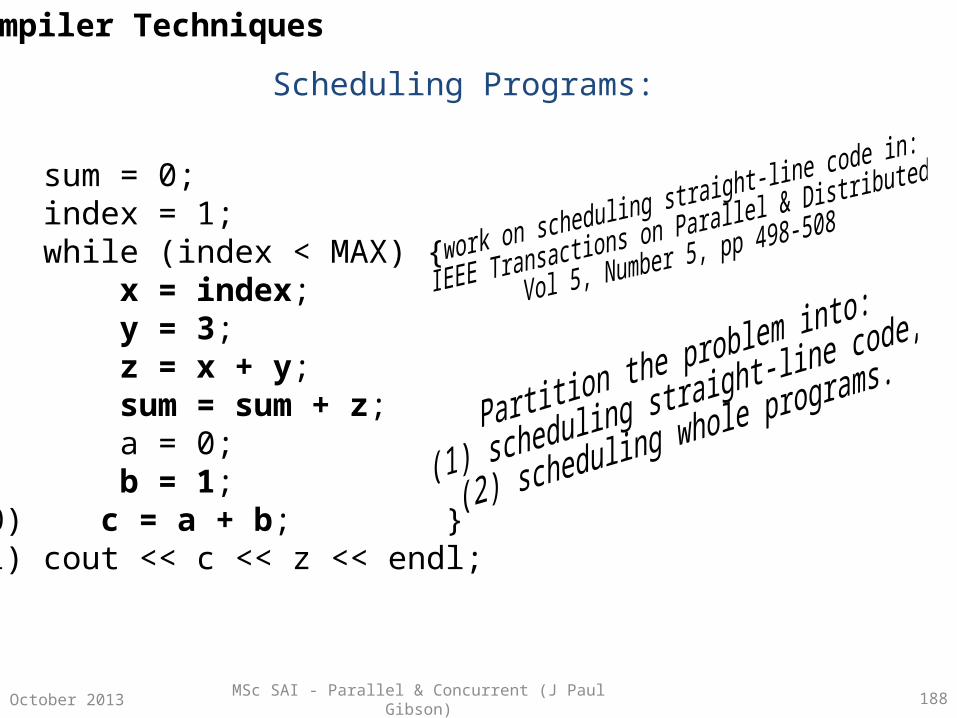
MSc SAI - Parallel & Concurrent (J Paul Gibson) 188October 2013
Scheduling Programs:
(1) sum = 0;(2) index = 1;(3) while (index < MAX) {(4) x = index;(5) y = 3;(6) z = x + y;(7) sum = sum + z;(8) a = 0;(9) b = 1;(10) c = a + b; }(11) cout << c << z << endl;
Compiler Techniques

MSc SAI - Parallel & Concurrent (J Paul Gibson) 189October 2013
Scheduling straight-line code for asynchronous execution is NP-Complete:
• First proven by B. Malloy– reduction from 3-SAT– 10 pages
• improved by E. Lloyd– reduction from 3-SAT– 5 pages
• reviewer– reduction from knapsack– 1 1/2 pages
Compiler Techniques
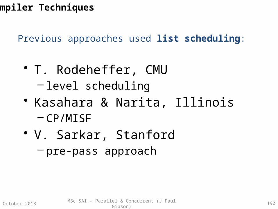
MSc SAI - Parallel & Concurrent (J Paul Gibson) 190October 2013
Previous approaches used list scheduling:
• T. Rodeheffer, CMU– level scheduling
• Kasahara & Narita, Illinois– CP/MISF
• V. Sarkar, Stanford– pre-pass approach
Compiler Techniques

MSc SAI - Parallel & Concurrent (J Paul Gibson) 191October 2013
Use a DAG to represent the code:
(4) x = index;(5) y = 3;(6) z = x + y;(7) sum = sum + z;(8) a = 0;(9) b = 1;(10) c = a + b;
= = sum
+
+
= =
+
Compiler Techniques

MSc SAI - Parallel & Concurrent (J Paul Gibson) 192October 2013
DAG: just the operations
(4) x = index;(5) y = 3;(6) z = x + y;(7) sum = sum + z;(8) a = 0;(9) b = 1;(10) c = a + b; 4 5 7.2
7.1
6
8 9
10
Compiler Techniques

MSc SAI - Parallel & Concurrent (J Paul Gibson) 193October 2013
Previous approaches used list scheduling:
• put all nodes into a list• schedule the list
• list construction
Compiler Techniques

MSc SAI - Parallel & Concurrent (J Paul Gibson) 194October 2013
List schedule the DAG;use level scheduling:
4 5 7.2
7.1
6
8 9
10
Compiler Techniques
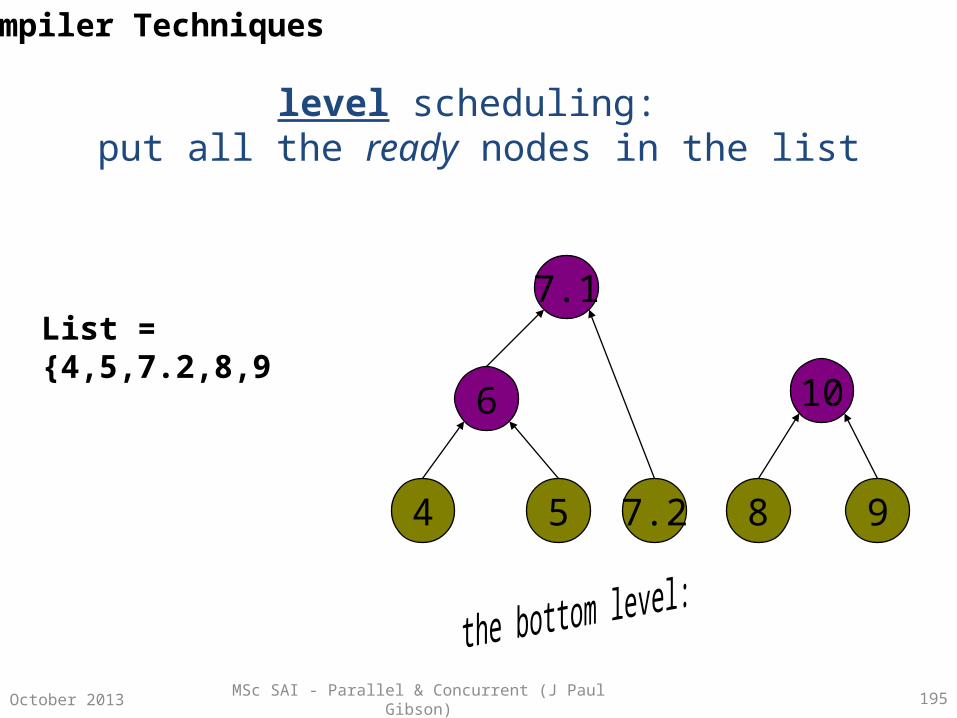
MSc SAI - Parallel & Concurrent (J Paul Gibson) 195October 2013
level scheduling: put all the ready nodes in the list
4 5 7.2
7.1
6
8 9
10
List = {4,5,7.2,8,9
Compiler Techniques
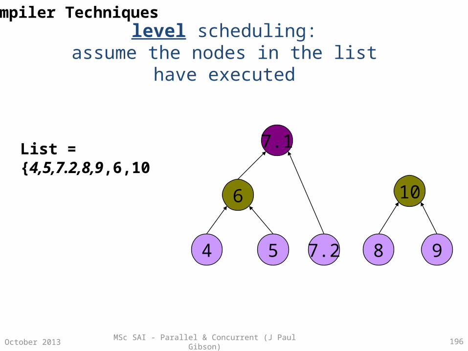
MSc SAI - Parallel & Concurrent (J Paul Gibson) 196October 2013
level scheduling:assume the nodes in the list have executed
4 5 7.2
7.1
6
8 9
10
List = {4,5,7.2,8,9,6,10
Compiler Techniques

MSc SAI - Parallel & Concurrent (J Paul Gibson) 197October 2013
level scheduling: get the last node
4 5 7.2
7.1
6
8 9
10
List = {4,5,7.2,8,9,6,10,7.1}
Compiler Techniques

MSc SAI - Parallel & Concurrent (J Paul Gibson) 198October 2013
assign nodes to processors:
List = {4,5,7.2,8,9,6,10,7.1}
p1 ={4,7.2,9,10}
p2 = {5,8,6,7.1}
Compiler Techniques

MSc SAI - Parallel & Concurrent (J Paul Gibson) 199October 2013
Assuming UET, construct schedule:
4 5 7.2
7.1
6
8 9
10
p1 ={4,7.2,9,10}
p2 = {5,8,6,7.1}
5 8 S8 W4 6 W7.2 7.1
4 S4 7.2 S7.2 9 W8 10
Compiler Techniques
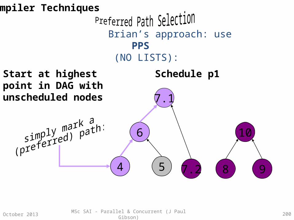
MSc SAI - Parallel & Concurrent (J Paul Gibson) 200October 2013
Brian’s approach: use PPS (NO LISTS):
Start at highest point in DAG with unscheduled nodes
Schedule p1
4 5 7.2
7.1
6
8 9
10
Compiler Techniques

MSc SAI - Parallel & Concurrent (J Paul Gibson) 201October 2013
PPS: choose a second preferred path
Schedule p2
Start at highest point in DAG with unscheduled nodes
4 5 7.2
7.1
6
8 9
10
Compiler Techniques
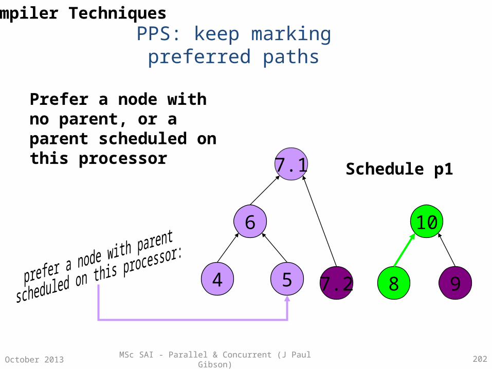
MSc SAI - Parallel & Concurrent (J Paul Gibson) 202October 2013
PPS: keep marking preferred paths
Prefer a node with no parent, or a parent scheduled on this processor
Schedule p1
4 5 7.2
7.1
6
8 9
10
Compiler Techniques

MSc SAI - Parallel & Concurrent (J Paul Gibson) 203October 2013
PPS: keep marking preferred paths
Prefer a node with no parent, or a parent scheduled on this processor
Schedule p2
4 5 7.2
7.1
6
8 9
10
Compiler Techniques

MSc SAI - Parallel & Concurrent (J Paul Gibson) 204October 2013
PPS: keep marking preferred paths
Prefer a node with no parent, or a parent scheduled on this processor
Schedule p1
4 5 7.2
7.1
6
8 9
10
Compiler Techniques

MSc SAI - Parallel & Concurrent (J Paul Gibson) 205October 2013
PPS: traverse DAG, build schedule;insert signal/wait if necessary:
4 5 7.2
7.1
6
8 9
10
4 5 7.2 6 7.1
8 9 10
Compiler Techniques
Results show technique scales reasonably well up to 8-16 processors/cores.
MSc SAI - Parallel & Concurrent (J Paul Gibson) 206October 2013
Compiler Techniques: Further Reading
B. A. Malloy, E. L. Lloyd, and M. L. Soffa. 1994. Scheduling DAG's for Asynchronous Multiprocessor Execution. IEEE Trans. Parallel Distrib. Syst. 5, 5 (May 1994)
Georgios Tournavitis, Zheng Wang, Bjorn Franke, and Michael F.P. O'Boyle. 2009. Towards a holistic approach to auto-parallelization: integrating profile-driven parallelism detection and machine-learning based mapping. SIGPLAN Not. 44, 6 (June 2009), 177-187
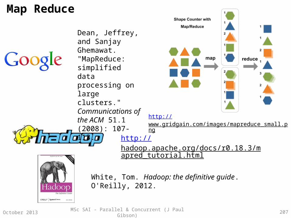
MSc SAI - Parallel & Concurrent (J Paul Gibson) 207October 2013
Map Reduce
http://hadoop.apache.org/docs/r0.18.3/mapred_tutorial.html
Dean, Jeffrey, and Sanjay Ghemawat. "MapReduce: simplified data processing on large clusters." Communications of the ACM 51.1 (2008): 107-113.
http://www.gridgain.com/images/mapreduce_small.png
White, Tom. Hadoop: the definitive guide. O'Reilly, 2012.
MSc SAI - Parallel & Concurrent (J Paul Gibson) 208October 2013
Development Tools/Environments/Systems
Open MPI - http://www.open-mpi.org/
Open MP - http://openmp.org/wp/
mpiJava - http://aspen.ucs.indiana.edu/pss/HPJava/mpiJava.html
SWARM - http://multicore-swarm.sourceforge.net/
See also:
java.util.concurrent for Java 7http://download.oracle.com/javase/7/docs/api/java/util/concurrent/package-summary.html
The Caml Hump: System :: Distributed and parallel programminghttp://caml.inria.fr/cgi-bin/hump.en.cgi?sort=0&browse=77