October 12, 2018 Mr. Brent J. Fields, - SEC.gov | HOME · fraction of the votes, but whether this...
47
October 12, 2018 Mr. Brent J. Fields, Secretary Securities and Exchange Commission 100 F Street, NE Washington, DC 20549-1090 via SEC internet submission form Re: File No. 4-725 -SEC Staff Roundtable on the Proxy Process Dear Mr. Fields, We are Nadya Malenko, Associate Professor of Finance at Boston College, Carroll School of Management, and Yao Shen, Assistant Professor of Finance at Baruch College, Zicklin School of Business. We are aware that the SEC is seeking responses on the role of proxy advisors in the proxy voting process. Motivated by multiple discussions and controversy about the influence of proxy advisory firms, and ISS in particular, we have written a research article titled “The role of proxy advisory firms: Evidence from a regression-discontinuity design,” published in the Review of Financial Studies in 2016. In our paper, we examine the effect of ISS recommendations on shareholder voting outcomes. There has been considerable disagreement about the extent of proxy advisors’ influence on shareholder votes. While the literature finds a strong positive correlation between proxy advisors’ recommendations and voting outcomes, estimating the true causal influence of proxy advisors is difficult. This is because if a proxy advisor recommends voting against a proposal, and that proposal is subsequently defeated, it does not necessarily imply that the proxy advisor’s negative recommendation was the reason for the defeat. Instead, it may be that the proposal is inherently detrimental to the firm, leading, simultaneously, to shareholders voting against it and to a negative recommendation from the proxy advisor. This difficulty in distinguishing correlation from causality has been widely recognized both in the academic literature and among industry participants, and was discussed at the SEC roundtable on proxy advisors in December 2013. As a result, many observers believe that the influence of proxy advisors is significantly overstated. In our paper, we provide causal estimates of the effect of ISS on voting outcomes for say-on-pay proposals over 2010-2011. Our empirical design uses a well-known econometric technique called Regression Discontinuity, by exploiting a cutoff rule that was used by ISS in its recommendations on say-on-pay proposals. The logic behind the Regression Discontinuity approach in our paper is the following: When analyzing say-on-pay proposals over 2010-2011, ISS used a cutoff rule to perform an initial screen: if a firm’s 1-year and 3-year Total Shareholder Return (TSR) were below certain cutoffs (industry median TSRs), ISS performed a deeper analysis of the firm’s compensation practices and, as a result,
Transcript of October 12, 2018 Mr. Brent J. Fields, - SEC.gov | HOME · fraction of the votes, but whether this...

October 12, 2018
Mr. Brent J. Fields,
Secretary Securities and Exchange Commission
100 F Street, NE Washington, DC 20549-1090
via SEC internet submission form
Re: File No. 4-725 -SEC Staff Roundtable on the Proxy Process
Dear Mr. Fields,
We are Nadya Malenko, Associate Professor of Finance at Boston College, Carroll School of
Management, and Yao Shen, Assistant Professor of Finance at Baruch College, Zicklin School of
Business.
We are aware that the SEC is seeking responses on the role of proxy advisors in the proxy voting process.
Motivated by multiple discussions and controversy about the influence of proxy advisory firms, and ISS
in particular, we have written a research article titled “The role of proxy advisory firms: Evidence from
a regression-discontinuity design,” published in the Review of Financial Studies in 2016.
In our paper, we examine the effect of ISS recommendations on shareholder voting outcomes. There has
been considerable disagreement about the extent of proxy advisors’ influence on shareholder votes.
While the literature finds a strong positive correlation between proxy advisors’ recommendations and
voting outcomes, estimating the true causal influence of proxy advisors is difficult. This is because if a
proxy advisor recommends voting against a proposal, and that proposal is subsequently defeated, it does
not necessarily imply that the proxy advisor’s negative recommendation was the reason for the defeat.
Instead, it may be that the proposal is inherently detrimental to the firm, leading, simultaneously, to
shareholders voting against it and to a negative recommendation from the proxy advisor.
This difficulty in distinguishing correlation from causality has been widely recognized both in the
academic literature and among industry participants, and was discussed at the SEC roundtable on proxy
advisors in December 2013. As a result, many observers believe that the influence of proxy advisors is
significantly overstated.
In our paper, we provide causal estimates of the effect of ISS on voting outcomes for say-on-pay
proposals over 2010-2011. Our empirical design uses a well-known econometric technique called
Regression Discontinuity, by exploiting a cutoff rule that was used by ISS in its recommendations on
say-on-pay proposals. The logic behind the Regression Discontinuity approach in our paper is the
following:
When analyzing say-on-pay proposals over 2010-2011, ISS used a cutoff rule to perform an initial
screen: if a firm’s 1-year and 3-year Total Shareholder Return (TSR) were below certain cutoffs (industry
median TSRs), ISS performed a deeper analysis of the firm’s compensation practices and, as a result,

was more likely to give a negative recommendation. In general, whether TSR is above or below the
cutoff could be correlated with the quality of the firm’s compensation practices: for example, poorly performing firms could be more likely to have poor compensation contracts. However, whether a firm
is just above the cutoff (i.e., in the 51st percentile of TSR) or just below the cutoff (i.e., in the 49th
percentile of TSR) is essentially random and is uncorrelated with proposal quality. This randomness
introduces an exogenous shock to ISS recommendations and allows us to provide a causal estimate of
ISS influence. We therefore compare firms that were just above the cutoff to those that were just below,
leading to the following main findings:
Relative to a positive recommendation, a negative ISS recommendation leads to a 25 percentage
point decrease in voting support for say-on-pay proposals over 2010-2011. In other words, ISS
moves about a quarter of the votes in our sample.
The influence of ISS is stronger in firms in which institutional ownership is larger and less
concentrated and in which there are more institutions that have high turnover or small positions. This
evidence is consistent with the idea that smaller and more short-term shareholders have stronger
incentives to rely on ISS instead of performing independent governance research.
We discuss the generalizability of our causal estimates beyond our sample and discuss that, under
certain assumptions, the 25% effect could be generalized to other firms and to subsequent years.
Overall, our findings indicate that ISS recommendations have a strong effect on voting outcomes,
especially in firms whose shareholders do not have incentives to conduct independent governance
research. While our paper does not evaluate whether this influence is good or bad, it emphasizes that,
contrary to frequent claims, the influence of ISS does not seem overstated, suggesting that the
consideration of various regulatory proposals is warranted.
We attach a copy of our paper, which contains the research underlying the above conclusions.
Sincerely,
Nadya Malenko Yao Shen
Associate Professor of Finance Assistant Professor of Finance
and Giuriceo Family Faculty Fellow Zicklin School of Business
Boston College, Carroll School of Management Baruch College, CUNY

The Role of Proxy Advisory Firms:
Evidence from a Regression-Discontinuity Design∗
Nadya Malenko Yao Shen
Boston College Baruch College
Review of Financial Studies, Vol. 29, No. 12, December 2016
Abstract
Proxy advisory firms have become important players in corporate governance, but the
extent of their influence over shareholder votes is debated. We estimate the effect of Insti-
tutional Shareholder Services (ISS) recommendations on voting outcomes by exploiting
exogenous variation in ISS recommendations generated by a cutoff rule in ISS voting
guidelines. Using a regression discontinuity design, we find that from 2010 to 2011, a
negative ISS recommendation on a say-on-pay proposal leads to a 25 percentage point
reduction in say-on-pay voting support, suggesting a strong influence over shareholder
votes. We also use our setting to examine the informational role of ISS recommendations.
(JEL G34, D72, J33, M12)
∗We are grateful to Itay Goldstein (the editor), two anonymous referees, Bernard Black, Mary Ellen Carter, Sudheer Chava, Alan Crane (discussant), Fabrizio Ferri (discussant), Cesare Fracassi, Mariassunta Giannetti, Amy Hutton, Dirk Jenter, Oguzhan Karakas, Darren Kisgen, Camelia Kuhnen, Doron Levit, Michelle Lowry, Andrey Malenko, Gregor Matvos (discussant), Anna Mikusheva, Jordan Nickerson, Jeffrey Pontiff, Jonathan Reuter, Miriam Schwartz-Ziv, Philip Strahan, Jerome Taillard, and Eric Zitzewitz (discussant) and participants at the 2015 Texas Finance Festival, the 2015 Ohio State University Corporate Finance Conference, the 2015 SFS Finance Cavalcade, the 2015 University of Oregon Summer Finance Conference, and seminar participants at Boston College, McGill University, University of California, Davis, and University of Pennsylvania for helpful comments and discussions. We are also grateful to Fabrizio Ferri for providing us with the data and to Jun Crystal Yang and Pouyan Foroughi for research assistance. Send correspondence to Nadya Malenko, Boston College, Fulton Hall 332, 140 Commonwealth Avenue, Chestnut Hill, MA 02467; telephone: (617) 552-2178. E-mail: [email protected].
1

Shareholder voting plays a key role in corporate governance. It has become especially important
because of the increase in institutional ownership, the rise in shareholder activism, the shift to
majority voting for director elections, and the introduction of mandatory say-on-pay. A significant
development in recent years has been the growth of proxy advisory firms. Proxy advisors counsel
investors on how to vote their shares on major corporate decisions, such as mergers and acquisitions,
director elections, executive compensation, and corporate governance policies. The largest proxy
advisor, Institutional Shareholder Services (ISS), covers almost 40,000 meetings in 115 countries and
has over 1,600 institutional clients.
Over time, regulators and market participants have become increasingly concerned with the influ-
ence proxy advisors allegedly have on investors’votes. According to the SEC commissioner Michael
Piwowar, at the 2013 SEC roundtable on proxy advisors, “proxy advisory firms may exercise out-
sized influence on shareholder voting” and the “Dodd-Frank provisions, such as mandatory say-on-
pay votes, make proxy advisory firms potentially even more influential.”Proxy advisors’ influence
is potentially concerning because their recommendations are frequently criticized for inaccuracies, a
one-size-fits-all approach to governance matters, and conflicts of interest stemming from the consult-
ing services to corporations.
Motivated by these concerns, the SEC has held several discussions about the role of proxy advisors;
these discussions culminated in the release of Staff Legal Bulletin No. 20 (SLB 20) in June 2014.
The main goal of the bulletin has been to provide guidance on investment advisors’ use of proxy
advisors and on proxy advisors’responsibilities in dealing with conflicts of interest. However, many
market participants, including regulators themselves, feel that the guidance provided by SLB 20 is
insuffi cient and that more stringent regulation may be necessary.1
To understand whether increased regulation is warranted, we must ultimately understand the
extent of proxy advisors’influence over shareholder votes. There is disagreement about whether the
impact of their recommendations is as strong as is sometimes claimed. On the one hand, regula-
tors’concerns about proxy advisors’, and especially ISS’s, outsized influence are consistent with the
1For example, the SEC commissioner Daniel Gallagher writes “While these reforms are much-needed, I am concerned that the guidance does not go far enough” (Gallagher 2014). See the Online Appendix for a more detailed discussion of the regulatory debate on proxy advisors.
2
strong positive correlation observed between ISS recommendations and voting outcomes. On the
other hand, assessing the actual influence of ISS has been diffi cult because of the omitted variable
problem: the same unobservable firm and management characteristics that lead ISS to give a negative
recommendation can also lead shareholders to withdraw their support for the proposal, leading to an
upward bias in the estimates of the ISS effect. This issue has been widely recognized in the academic
literature and by many industry participants and has been discussed at the SEC roundtable on proxy
advisors in December 2013. Prior literature concludes that ISS recommendations move at least some
fraction of the votes, but whether this fraction is large or small remains unclear (e.g., Iliev and Lowry
2015; Ertimur, Ferri, and Oesch 2013; Larcker, McCall, and Ormazabal 2015).2 As a result, many
observers believe that the influence of proxy advisors is significantly overstated and hence believe
that stringent regulation may do more harm than good (e.g., Edelman 2013). Even ISS itself has
used this argument to alleviate regulators’concerns about its oversized influence and prevent further
regulation (ISS 2012): “As many investors can be expected to share a general approach to assessing
corporate governance practices, it is perhaps not surprising that correlations can be found between
ISS recommendations and shareholder voting outcomes. However, this does not prove causality, nor
are those correlations consistent. In our view, it is more logical to interpret broad correlation as
indicating that ISS policies, analyses and recommendations are based on principles and approaches
which are shared by many investors.”
In this paper, we address this empirical challenge and quantify the causal effect of ISS by ex-
ploiting exogenous variation in ISS recommendations due to a cutoff rule employed by ISS in its
2010-2011 guidelines on say-on-pay proposals. Specifically, ISS used to conduct an initial screen of
companies focusing on their one- and three-year total shareholder returns (TSRs) relative to certain
cutoffs and only performed a deeper analysis of the company’s executive compensation practices for
companies below the cutoff. For example, the ISS 2012 white paper “Evaluating Pay for Performance
Alignment” notes “In the last few years, the approach has utilized a quantitative methodology to
2For example, Iliev and Lowry (2015), Ertimur, Ferri, and Oesch (2013), and Larcker, McCall, and Ormaz-abal (2015) show that sensitivity to ISS recommendations is weaker for shareholders that are larger and have lower turnover, and Ertimur, Ferri, and Oesch (2013) use this differential sensitivity to put a lower bound on the causal effect of ISS.
3

identify underperforming companies — i.e., those with both 1- and 3-year total shareholder return
(TSR) below the median of peers in their 4-digit Global Industry Classification Standard (GICS)
group. Underperforming companies then received an in-depth qualitative review, focused primarily
on factors such as the year-over-year change in the CEO’s total pay, the 5-year trend in CEO pay
versus company TSR, and the strength of performance-based pay elements.”More specifically, as we
discuss in Section 2.1, the cutoff for a given company is calculated as the median TSR of all firms
that are both in the company’s four-digit GICS industry group and in Russell 3000, where the TSRs
are computed on the last day of the calendar quarter closest to the company’s fiscal year-end. In the
rest of the paper, we refer to this rule as the ISS “cutoff rule”.
The ISS cutoff rule allows us to use a regression discontinuity (RD) design to estimate the causal
effect of ISS recommendations on say-on-pay voting outcomes. Specifically, the rule implies that firms
below the cutoff undergo more scrutiny to achieve a positive recommendation from ISS than firms
above the cutoff, and hence the probability of a negative ISS recommendation should increase discon-
tinuously just below the cutoff. Indeed, we show that relative to firms just above the cutoff, there is a
15% increase (from 10% to 25%) in the probability of a negative say-on-pay recommendation for firms
just below the cutoff. This jump is large given that the average probability of a negative say-on-pay
recommendation in our sample is 12.7%. At the same time, the somewhat arbitrary nature of the ISS
cutoff suggests that being just above or below the cutoff is locally random, that is, firms around the
cutoff are similar across all characteristics, except for, potentially, the ISS recommendation. Thus,
any discontinuous decrease in voting support below the cutoff can be attributed to the discontinuity
in ISS recommendations; this allows us to implement a fuzzy RD design to estimate the causal effect
of ISS (Imbens and Lemieux 2008; Roberts and Whited 2012).
Our analysis shows a strong effect of ISS recommendations on say-on-pay voting outcomes: we
find that relative to positive recommendations, negative ISS recommendations lead to a 25 percentage
point decrease in voting support for say-on-pay proposals from 2010 to 2011. In other words, ISS
moves about a quarter of the votes in our sample. This effect is economically significant: dissent
above 20% is viewed as an indication of substantial dissatisfaction (e.g., Del Guercio, Seery, and
Woidtke 2008; Ferri and Maber 2013) and leads companies to change their compensation practices
4

(Ferri and Maber 2013; Ertimur, Ferri, and Oesch 2013). Our main specification is a local linear
regression estimated on a 5% bandwidth, and our estimates are robust to using multiple bandwidths
and flexible polynomial functions and to controlling for various firm characteristics. We also show
that the influence of ISS is stronger in firms in which institutional ownership is larger and less
concentrated and in which there are more institutions that have high turnover or small positions,
consistent with the hypothesis that such shareholders have stronger incentives to rely on ISS instead
of performing independent governance research (e.g., Iliev and Lowry 2015).
The key assumption of our RD design is that whether a firm falls just above or below the cutoff is
locally random. We perform several tests to verify this assumption and show that our results are not
driven by differences in firm characteristics around the cutoff. First, we redo our analysis on several
samples for which the ISS cutoff rule does not apply: say-on-pay voting in 2012 (the year in which
ISS stopped using this rule), voting for the board as a whole, and voting for compensation committee
members. In all these samples, voting support is continuous around the cutoff, suggesting that the
discontinuity in votes in our main sample exists because of the corresponding discontinuity in ISS
recommendations. Second, we show that the distribution of various elements of CEO compensation
and other firm characteristics is smooth around the cutoff. Third, we alleviate the concern that
firms manipulate their TSRs to move above the cutoff by performing the McCrary (2008) test and
showing that the density of the forcing variable is smooth around the cutoff. Such manipulation is
indeed unlikely, given that the cutoff depends on the TSRs of all firms in the industry and the TSRs
are determined by stock price movements. Fourth, we consider several placebo cutoffs and show
continuity in voting support around them.
We also use our results to discuss the informativeness of ISS recommendations relative to the
information that shareholders possess independently. To study this question, we compare our esti-
mates of ISS’s influence to the estimates obtained via ordinary least squares (OLS) and find that
the two are very close to each other. As we discuss in Section 5.1, this result suggests that if large
long-term shareholders perform their own governance research and vote based on it (as prior liter-
ature suggests), then ISS recommendations are uncorrelated with these shareholders’ information.
For example, this could be the case if large shareholders perform firm-specific research, while ISS
5
follows a one-size-fits-all approach to governance matters.
Finally, we discuss the generalizability of our results beyond our sample. The RD design does not
allow us to estimate the causal effect of ISS for other types of proposals or for firms away from the
cutoff and after 2011, so one should be cautious in extrapolating our estimates to the general effect
of ISS recommendations. However, we examine the OLS estimates of the ISS effect on say-on-pay
voting outcomes and find that they are very stable across different subsamples from 2010 to 2011
(ranging between 23% and 25%) and over time (ranging between 25% and 29%). Assuming that the
omitted variable bias in OLS estimates remains small in these other samples, this suggests that the
25% effect could be generalized to other firms and to subsequent years.
Our paper contributes to the literature on shareholder activism and the role of institutional
investors in firms’corporate governance.3 In particular, it is related to the literature on shareholder
voting. Prior research shows that shareholder voting has a significant impact on firms’policies and
value, even when votes are nonbinding.4 Cuñat, Gine, and Guadalupe (2012, 2015) find that relative
to proposals that fail by a small margin, proposals that pass by a small margin yield an abnormal
return between 1.3% and 2.4%, depending on the proposal type. In the context of say-on-pay voting,
Ferri and Maber (2013) show that about 80% of U.K. firms with substantial voting dissent respond
by removing controversial compensation practices, and Ertimur, Ferri, and Oesch (2013) find similar
evidence for U.S. firms.5 Given the significance of shareholder voting, it is important to understand
which factors affect investors’voting decisions. Our paper shows that the recommendations of proxy
advisory firms are a major factor affecting shareholder votes.
The literature on proxy advisors documents a significant positive association between ISS rec-
ommendations and shareholder support on various voting issues.6 Many papers point out that the
3For example, Hartzell and Starks (2003), Aghion, Van Reenen, and Zingales (2013), Mullins (2014), Boone and White (2015), Appel, Gormley, and Keim (2016), and Crane, Michenaud, and Weston (2016). See Karpoff (2001), Gillan and Starks (2007), and Brav, Jiang, and Kim (2009) for reviews of the literature on shareholder activism.
4See Ferri (2012) for a survey of nonbinding voting and Levit and Malenko (2011) for a theoretical analysis. 5Relatedly, Schwartz-Ziv and Wermers (2015) show that low say-on-pay support is followed by a decrease
in excess compensation and better selection of peer firms when ownership is relatively concentrated. See also Ertimur, Ferri, and Muslu (2011) and Cai and Walkling (2011).
6See, for example, Alexander et al. (2010), Bethel and Gillan (2002), Cai, Garner, and Walking (2009), Morgan et al. (2011), Ertimur, Ferri, and Oesch (2013, 2015), Aggarwal, Erel, and Starks (2015), Iliev and Lowry (2015), and Larcker, McCall, and Ormazabal (2015).
6

association between recommendations and vote outcomes might not be causal and might be ex-
plained by shareholders and ISS independently reaching the same conclusions and/or by ISS being
influenced by institutional investors’opinions. To assess causality, Iliev and Lowry (2015), Ertimur,
Ferri, and Oesch (2013), and Larcker, McCall, and Ormazabal (2015) show that sensitivity to ISS
recommendations is stronger for shareholders that are smaller and have higher turnover, consistent
with these shareholders having weaker incentives to perform independent research. Using this differ-
ential sensitivity to ISS, Ertimur, Ferri, and Oesch (2013) estimate that, under certain assumptions
on blockholder versus nonblockholder voting, the lower bound on the causal effect of ISS is 5.7%,
while the upper bound is 25%, their OLS estimate.7 Thus, prior literature suggests that ISS moves
at least some fraction of the votes, but it is unknown whether this effect is small (in the order of
magnitude of 5%) or large (in the order of magnitude of 25%). Our main contribution to this liter-
ature is to estimate the magnitude of the causal effect of ISS. We show that ISS recommendations
move 25% of say-on-pay votes; this is evidence of rather strong influence. In addition, this effect is
similar to the estimates obtained via OLS, suggesting that at least based on our sample of 2010-2011
say-on-pay votes, the influence of ISS does not seem overstated. In a contemporaneous study, Bach
and Metzger (2015) use the passing of shareholder proposals as an instrument for ISS recommenda-
tions on directors and estimate the ISS effect to be 25% as well. Motivated by the evidence on ISS’s
influence, Malenko and Malenko (2016) provide a theoretical analysis of the effect of proxy advisors
on voting outcomes.
1 Methodology
In this section, we discuss how we use the regression discontinuity design to estimate the causal effect
of ISS recommendations on say-on-pay voting outcomes.
According to the ISS cutoff rule, companies identified as “underperforming”, that is, whose both
7The lower bound is calculated under the assumptions that all institutional blockholders do their own research and cast votes independently of ISS and that all shareholders (blockholders and nonblockholders) doing their own research reach, on average, the same conclusions. In a similar spirit, Choi, Fisch, and Kahan (2010) study the interaction terms between ISS recommendations and individual and institutional investor holdings. Assuming that voting of individual investors is a perfect proxy for how institutions would vote if ISS did not exist, they conclude that the causal effect of ISS is between 6% and 10%.
7

one- and three-year TSRs are below the respective median TSRs of their four-digit GICS groups,
receive an in-depth qualitative review of their compensation practices from ISS. This rule suggests
that ISS is likely to give a positive say-on-pay recommendation without conducting deep analysis if
the firm is not identified as “underperforming”, but will carefully scrutinize the firm’s compensation
practices before giving it a positive recommendation if the firm is “underperforming”. As we show
in Section 3.1, this leads to a discrete jump in the probability of a negative recommendation for
“underperforming” firms. We therefore implement a fuzzy RD design by instrumenting a negative
ISS recommendation with an indicator variable BelowCutoff , which equals one if the firm’s one- and
three-year TSRs both fall below their respective industry medians, and zero otherwise (Imbens and
Lemieux 2008; Roberts and Whited 2012). Formally, for firm i in year t, BelowCutoff it is given by
⎧ ⎪⎨ 1 if MaxT SRit < 0, BelowCutoff it = (1)⎪⎩ 0 otherwise,
where MaxT SR is the forcing variable, measured in percentage points and defined as
MaxT SRit = max(TSR(1) − MedianTSR(1) , TSR(3) − MedianTSR(3)), (2)it it it it
(n) (n)TSR is the n-year TSR of firm i computed in year t, and MedianT SR is the median n-year it it
TSR in year t computed across all Russell 3000 firms in the same four-digit GICS group as firm i.
The identification assumption is local continuity, which implies that firms around the cutoff are
comparable, so that the relation between voting support and the variable MaxT SR would be smooth
around the cutoff in the absence of differential ISS recommendations. This assumption is plausible
because the cutoff used by ISS is somewhat arbitrary. First, it is based on the TSRs of a specific
group of firms (those both in Russell 3000 and in the firm’s four-digit GICS group), and second,
the TSRs are calculated on a specific date (the last day of the quarter closest to the firm’s fiscal
year-end). We further discuss and formally test this identification assumption in Sections 4.2-4.4.
We conduct the two-stage least-squares (2SLS) procedure by estimating the following two-equation
8

system. The first (second) equation corresponds to the first (second) stage:
NegRec = γ0 + γ1BelowCutoff + f1(MaxTSR) + BelowCutoff · f2(MaxTSR) + γX + u, (3)
\Votes = α0 + α1NegRec + g1(MaxTSR) + BelowCutoff · g2(MaxTSR) + αX + ε,
where Votes is the percentage of votes in favor of a say-on-pay proposal; NegRec is an indicator
variable equal to one if the ISS recommendation is negative and zero if positive; \NegRec is the
fitted value of NegRec from the first-stage regression; f1, f2, g1, and g2 are continuous functions of
MaxT SR; and X is a vector of control variables. As is standard in the literature (e.g., Imbens and
Lemieux 2008), we estimate a linear probability model for the first stage. The key coeffi cient of
interest is α1, which captures the local average treatment effect of a negative ISS recommendation
on voting support. Standard errors are computed as the usual 2SLS standard errors.
Our main specification is a local linear regression, that is, fi and gi are linear functions, and the
regressions are estimated on a small bandwidth around the cutoff, −h < MaxTSR < h. Section
4.1 shows that results are robust to including higher-order polynomials. Following the practical
considerations in Imbens and Lemieux (2008), we focus on the rectangular kernel and use the same
bandwidth for both stages. The trade-off in choosing the bandwidth is that a larger bandwidth
increases precision by including more observations, but introduces an additional bias. In the main
analysis, we use the bandwidth of 5%. Section 4.1 shows that our estimates are robust to bandwidth
choice. We also apply the cross-validation procedure, which is commonly used to determine the
optimal bandwidth (see the Online Appendix for details). The cross-validation procedure yields the
optimal bandwidth between 4% and 5%, consistent with our baseline bandwidth of 5%.
In model 1 of Tables 2 and 3, we restrict the slope of the linear regression so that it is the same on
the two sides of the cutoff, and in models 2-5, we allow for different slopes around the cutoff. Note
that as long as the covariates are continuous around the cutoff (the assumption that we verify for
various firm characteristics in Section 4.3), fuzzy RD design does not require the inclusion of control
variables other than the forcing variable to produce consistent estimates (Imbens and Lemieux 2008).
Nevertheless, we include several firm characteristics that may affect support for say-on-pay proposals,
such as characteristics of the executive pay package, the firm’s ownership structure, and other firm
9
characteristics, as well as year and industry fixed effects, and show the robustness of our results.
2 Data and Variable Construction
The data on ISS recommendations and voting outcomes come from the ISS Voting Analytics database,
which covers Russell 3000 firms. For each firm and each proposal on the agenda, the database provides
the ISS recommendation, the percentage of votes for, votes against, and abstentions, and whether
the proposal passed or failed. There is variation across firms in the way voting support is calculated.
While the numerator is always the number of votes in favor of the proposal, the denominator, captured
by the variable “base”, is different across firms. Base can be the sum of the votes in favor and against
(51.83% of the sample), the sum of the votes in favor and against plus the number of abstentions
(47.77% of the sample), or the number of shares outstanding (0.40% of the sample). We use the
appropriate denominator to calculate Votes, the percentage voting support for each company.
We obtain the data on TSRs and firm characteristics from Compustat, the data on institutional
ownership from Thomson Reuters 13F, the data on executive compensation and insider ownership
from GMI Ratings (formerly Corporate Library), and the list of Russell 3000 firms from Bloomberg.
We first match the ISS sample to Compustat and CRSP by ticker and company name.8 We then
merge the sample with GMI Ratings by ticker and name, and with Thomson Reuters 13F by CUSIP,
name, and ticker. The Appendix contains the definitions of the variables used in the paper.
For most of the analysis, except for the falsification tests in Section 4.4, we focus on say-on-pay
proposals voted on in 2010 and 2011, the years in which ISS applied its cutoff rule. Even though
the cutoff rule might have been used prior to 2010, we did not find a formal mention of this rule in
the 2007-2009 ISS guidelines. We do not lose many observations by excluding prior years because
say-on-pay proposals were relatively rare before 2011, at which point they were made mandatory by
the Dodd-Frank Act. 8We conduct two rounds of matching to ensure that the match is correct. The first approach is to merge
the data with Compustat to obtain GVKEY (and CUSIP) and then merge with the CRSP/COMPUSTAT Merged link table to get PERMNO (and CUSIP). The second approach is to first merge the data with the stock names file from CRSP to get PERMNO and then merge with the link table to obtain GVKEY. We cross-check the observations after the two rounds of matching.
10

2.1 Constructing the TSR cutoffs
The Online Appendix presents a detailed description of the ISS cutoff rule, and we summarize the
relevant information here.
According to the ISS guidelines, “ISS utilizes S&P’s Compustat database for TSR calculated
values. The Total Return concepts are annualized rates of return reflecting price appreciation plus
reinvestment of dividends (calculated monthly) and the compounding effect of dividends paid on
reinvested dividends.”We therefore also use Compustat’s Total Return concept to calculate TSRs. In
particular, we multiply the current month’s adjusted close price by the current month’s Total Return
Factor provided by Compustat, divide the result by the product of the adjusted close price multiplied
by the Total Return Factor from the prior period (one or three prior years for T SR(1) and T SR(3),
respectively), and annualize the three-year return. The Total Return Factor is a multiplication factor
that reflects monthly price appreciation and reinvestment of monthly dividends and cash equivalent
distributions and the compounding effect of dividends paid on reinvested dividends.
The one-year (three-year) TSR cutoff for each firm is calculated as the median one-year (three-
year) TSR of Russell 3000 firms in the same four-digit GICS industry. ISS guidelines specify the
following dates to compute TSRs. TSRs are downloaded at the end of each calendar quarter, that is,
on the last day of March, June, September, and December. For a given firm and year, the relevant
download date is the last day of the calendar quarter closest to the fiscal year-end of the subject firm.
For example, if a firm’s fiscal year-end is March 31, TSRs for firms in the same industry group are
calculated on March 31. Besides manually calculating the median industry TSRs, we obtain the list
of median TSRs from the ISS Web site. For illustration, the Online Appendix presents a screenshot
of the Web page with median TSRs for each industry group downloaded from 2014 to 2015. We
obtain similar tables for most periods in our sample and find that they mostly match our manually
calculated cutoffs. Because the medians from the ISS Web site more precisely capture the cutoffs
used by ISS, we use these medians for all quarters for which they were available on the ISS Web site
and use our manually calculated medians for the remaining quarters. For robustness, we repeated
the analysis using the manually calculated medians for all quarters and obtained similar results.
11

ISS guidelines do not specify whether a given firm’s TSR, which is compared to the industry
median cutoff, is downloaded on the firm’s fiscal year-end date or, similarly to the corresponding
industry median, at the end of the calendar quarter closest to its fiscal year-end. The two approaches
coincide for firms whose fiscal year-end falls on the end of the calendar quarter; this constitutes
90% of the sample. To follow the ISS methodology precisely, we restrict our sample to these 90% of
firms. We also note that regardless of the company’s TSRs, ISS always gives it a positive say-on-pay
recommendation if the total dollar value of CEO compensation is suffi ciently small, in particular,
below the fifth percentile of firms in that year. This implies that the fuzzy RD setting is not directly
applicable for this group of firms, so we restrict our sample to observations with the total value of
CEO compensation above the fifth percentile in that year. Our results are very close if we keep these
observations, and the only difference is that at the first stage, the discontinuity in the probability of
a negative ISS recommendation is slightly smaller.
2.2 Descriptive statistics
Our final sample covers 1,932 firms and 2,020 say-on-pay proposals in 2010 and 2011: 106 in 2010
and 1,914 in 2011, when say-on-pay became mandatory for a large number of firms.9 The number
of observations below the ISS cutoff (that is, with MaxT SR < 0) is 613; this constitutes 30% of the
sample. Panel A of Table 1 presents descriptive statistics of the sample firms. The average market
capitalization is $5.5 billion; the average institutional ownership is 72%; and the average value of
executive compensation is $4.8 million. Panel A also presents descriptive statistics for our main
subsample of firms in a 5% bandwidth around the cutoff (we discuss the comparison between the two
samples in Section 4.6). Panel B presents voting outcomes depending on the ISS recommendation.
The probability that ISS gives a negative recommendation is 12.7% (256 observations out of 2,020).
The average voting support is 93.2% if ISS gives a positive recommendation, and 68.9% if ISS
gives a negative recommendation. While all 1,764 proposals with a positive ISS recommendation
received more than 50% voting support and thus passed, 29 out of 256 proposals with a negative
9Say-on-pay proposals were not mandatory in 2010, but this does not affect our methodology: the factors that lead a say-on-pay proposal to be included in the agenda do not invalidate the RD design as long as they are continuous around the cutoff.
12

recommendation failed. These statistics are consistent with the strong positive association between
ISS recommendations and voting outcomes documented in prior studies. Next, we use the RD
approach to examine which part of this association is causal.
[TABLE 1 HERE]
3 Effect of ISS on Voting Outcomes
We first present the graphical analysis and then the results of the 2SLS estimation. Figure 1 plots
the distribution of ISS recommendations and voting support for say-on-pay proposals on a 10%
bandwidth around the cutoff. Visual inspection of the graphs reveals a discontinuity in both variables
around the cutoff: there is about a 20 percentage point increase in the probability of a negative ISS
recommendation and about a 5 percentage point decrease in say-on-pay voting support for firms
just below the cutoff relative to firms just above the cutoff. Given the identification assumption, we
attribute the discontinuity in votes to the causal effect of ISS recommendations. For comparison, we
find no similar discontinuity in votes for samples in which the ISS cutoff rule is not used, suggesting
that shareholders do not use the same cutoff for their voting decisions (see Section 4.4).
In a fuzzy RD design, the estimate of the causal effect of treatment is the ratio of the two
discontinuities, that is, the difference in expected outcomes around the cutoff divided by the difference
in the probability of treatment around the cutoff. Hence, our rough estimate of the causal effect of
5%ISS based on the graphical analysis is , or 25 percentage points. In the next sections, we formally20%
estimate the effect of ISS by conducting the 2SLS analysis in a narrow bandwidth.
[FIGURE 1 HERE]
3.1 Discontinuity of ISS recommendations around the cutoff
We start by formally showing the discontinuity in the probability of a negative ISS recommendation.
Table 2 reports the first-stage regression estimated on a 5% bandwidth. This sample contains 403
observations, with 175 of them corresponding to firms below the cutoff. Models 1 and 2 control for
13

the forcing variable with and without the interaction term, and model 3 adds year and industry fixed
effects. In models 4 and 5, we add additional control variables that have been used in the literature
on say-on-pay and proxy advisors (e.g., Ertimur, Ferri, and Oesch 2013). Specifically, in model 4, we
control for governance characteristics that are likely to affect ISS recommendations and say-on-pay
support: several characteristics of the executive compensation package, as well as institutional and
insider ownership.10 In model 5, we control for other firm characteristics, such as firm size, return on
assets (ROA), and market-to-book ratio. In all specifications, the coeffi cient on BelowCutoff is about
0.15, that is, the probability of a negative ISS recommendation for firms just below the cutoff is 15
percentage points higher than for firms just above the cutoff. In unreported results, we also estimate
the probit model for the first-stage regression. The marginal effect of the coeffi cient on BelowCutoff
is 0.13, which is consistent with the estimates from the linear probability model.
[TABLE 2 HERE]
The magnitude of the first-stage discontinuity is substantial. Indeed, negative ISS recommen-
dations are relatively rare: according to Table 1, the sample average probability of a negative rec-
ommendation is 12.7%. Therefore, the 15% jump around the cutoff is economically significant. In
Section 4.5, we examine the strength of this instrument in more detail.
3.2 Effect of ISS recommendations on voting support
By using the discontinuity in ISS recommendations as an instrument, we next analyze the effect
of ISS on voting outcomes. Table 3 presents the second-stage estimates for several specifications
corresponding to those in Table 2. Importantly, our estimates are not biased by any omitted variables
as long as these variables are continuous around the cutoff.
In models 1 and 2, the coeffi cient on NegRec is about -25 and is significant at the 5% level,
suggesting that relative to a positive recommendation, a negative ISS recommendation reduces say-
on-pay voting support by 25 percentage points. As expected under the identification assumption,
10 Since the say-on-pay vote is to approve executive compensation over the preceding fiscal year, we use compensation variables from the fiscal year preceding the fiscal year of the shareholder meeting.
14

the effect is quantitatively similar and remains significant once we include year and industry fixed
effects and other control variables: the coeffi cient on NegRec in model 5 is -26.6 and is significant at
the 5% level. In Section 4.1, we verify the robustness of this effect to the choice of the bandwidth
and the inclusion of higher-order polynomial controls.
It is instructive to compare the RD coeffi cients on NegRec to the coeffi cients from the corre-
sponding OLS regressions of Votes on NegRec. We present the OLS estimates, standard errors, and
p-values of the Durbin-Wu-Hausman test in the last three rows of Table 3. Interestingly, the OLS
estimates are very close to the RD estimates: they are about 25% across all specifications, which is
similar to the estimate in Ertimur, Ferri, and Oesch (2013) for say-on-pay proposals during the same
time period. The Durbin-Wu-Hausman test does not reject the hypothesis that the RD and OLS
estimates are equal. Thus, our estimate of the causal effect of ISS is very close to the upper bound
of 25% that was proposed by Ertimur, Ferri, and Oesch (2013) based on their evidence. We discuss
the implications of this finding in Section 5.1.
[TABLE 3 HERE]
The 25% effect is economically important. Indeed, practitioners and prior academic studies con-
sider voting dissent of above 20% to be an indication of strong shareholder dissatisfaction (e.g., Del
Guercio, Seery, and Woidtke 2008; Ferri and Maber 2013). According to a 2011 investor survey, 72%
of investor respondents believe that voting dissent above 30% warrants an explicit response from the
board regarding improvements in pay practices, and 20% is the most commonly cited dissent level
that should trigger such a response (see “2011-2012 Policy Survey Summary of Results” by ISS).
Accordingly, say-on-pay dissent above 20%-30% prompts most firms to change their compensation
policies. Ferri and Maber (2013) examine U.K. firms and show that about 80% of firms with more
than 20% say-on-pay dissent remove controversial pay practices, such as generous severance contracts
and problematic performance-based vesting conditions in equity grants. Similarly, Ertimur, Ferri,
and Oesch (2013) find that more than 70% of U.S. firms with at least 30% voting dissent change their
compensation policies following the vote. Schwartz-Ziv and Wermers (2015) find that companies with
low say-on-pay support are likely to decrease excessive compensation and pick peer firms that more
15

closely resemble their own company when ownership is concentrated.
Why do firms respond to low say-on-pay support? In the past, low support levels, and especially
failed votes, have led to shareholder lawsuits, negative media attention, and damage to firms’repu-
tation. In its guidelines, ISS notes that if a company fails to “adequately respond to the company’s
previous say-on-pay proposal that received the support of less than 70 percent of votes cast,” ISS
may recommend to vote against the members of the compensation committee and potentially the
full board. Similarly, Glass Lewis places extra scrutiny on firms with less than 75% approval. These
consequences, combined with the strong influence of ISS on voting outcomes that we document,
suggest that proxy advisors play an important role in firms’governance practices.
3.2.1 Variation in the effect of ISS across firms
The 25% estimate captures the impact of ISS on aggregate shareholder support and does not dis-
tinguish between different shareholders. In this section, we examine whether ISS has a particularly
strong influence on certain types of investors by studying how the effect of ISS varies with the firm’s
ownership structure. Of course, because ownership structure is determined endogenously, we should
be cautious about the interpretation of the cross-sectional results in this section.
We start by examining whether ISS has a smaller effect on shareholders that are ex ante more
likely to perform independent governance research. Iliev and Lowry (2015), Ertimur, Ferri, and Oesch
(2013), and Larcker, McCall, and Ormazabal (2015) show that sensitivity to ISS recommendations is
weaker for institutions that are larger, have a larger stake in the firm, and have lower turnover, con-
sistent with these investors having particularly strong incentives to invest in independent research.
To study similar questions in our data, we examine how the effect of ISS varies with several ownership
structure characteristics. First, in models 1-3 of Table 4, we look at several variables that measure
shareholder size or concentration: institutional ownership Herfindahl-Hirschman index, defined as
the sum of squared share ownership over all institutional investors; ownership by institutional block-
holders (that is, institutions with more than a 5% stake); and ownership by the top ten institutional
shareholders. The larger each of these variables is, the more likely that many shareholders have
incentives to perform independent research, so we expect the impact of ISS to be smaller. Second,
16

we follow Larcker, McCall, and Ormazabal (2015), who use the Bushee and Noe (2000) classification
of institutional investors into three types —“transient”, “quasi-indexer”, and “dedicated”. Larcker,
McCall, and Ormazabal (2015) hypothesize that “dedicated”institutions have stronger incentives to
acquire their own information, because of their large ownership blocks and low turnover, compared
with the two other institution types. They thus define an institution as “passive”(in its reliance on
ISS) if it is either “transient”or a “quasi-indexer”and, consistent with their hypothesis, show that
the effect of ISS is stronger when the ownership by “passive” institutions is higher. Therefore, we
also calculate the percentage of shares held by “passive”institutions and study its effect in model 4
of Table 4.
For each ownership characteristic, we restrict the sample to observations in a bandwidth around
the cutoff and calculate the median value of this ownership characteristic in the resulting sample.
Next, we divide this sample into two subsamples, based on whether the ownership characteristic falls
below or above the median, and repeat the RD analysis on each subsample. Because the sample size
drops twice when we cut the sample into these subsamples, we focus on a 10% bandwidth to avoid
losing power and to keep the size of each subsample similar to the sample size in our main tests. The
results are presented in Table 4. The coeffi cient on BelowCutoff in the first stage is consistent across
subsamples and is close to the 15% coeffi cient in Table 2. This is expected, given that the ISS cutoff
rule does not vary with the firm’s ownership structure. In contrast, the coeffi cient on NegRec in the
second stage is quite different across subsamples and is consistent with the hypothesis that ISS has a
weaker effect on shareholders who are more likely to do independent research. For example, the effect
of ISS is 41% and 21% for the subsamples with low and high institutional ownership concentration,
respectively. Similarly, the effect of ISS is 38% and 19% for firms with high and low ownership by
“passive” institutions, respectively. These results are in line with the findings of Iliev and Lowry
(2015), Ertimur, Ferri, and Oesch (2013), and Larcker, McCall, and Ormazabal (2015).
Finally, in model 5 of Table 4, we examine the difference between institutional investors and
other types of shareholders, such as retail investors or insiders. We expect ISS to have a particularly
strong influence on the votes of institutional investors, who are its main clients. Consistent with this
hypothesis, the coeffi cient on NegRec is -24.1 and -32.3 for the low and high institutional ownership
17

subsamples, respectively.
[TABLE 4 HERE]
4 Validity of the RD Design and Robustness
In this section, we perform additional tests to show the validity of our RD setting. Section 4.1
analyzes the robustness of the estimates, Sections 4.2—4.4 present tests of internal validity, Section
4.5 examines the strength of the instrument, and Section 4.6 discusses external validity.
4.1 Robustness
We start by showing the robustness of our results to alternative bandwidths and specifications. The
first two rows of Table 5 present the estimate and standard error of the coeffi cient on BelowCutoff
in the first-stage regression, and the third and fourth rows present the estimate and standard error
of the coeffi cient on NegRec in the second-stage regression. In columns 1-8, we repeat the analysis of
the third specification from Tables 2 and 3 on bandwidths ranging between 3% and 10% and show
that the estimates for both the first and second stages are quantitatively similar across bandwidths
(results for other specifications are similar and omitted for brevity). An alternative to estimating
a local linear regression on a narrow bandwidth is to use a larger sample but include higher-order
polynomials of the forcing variable (e.g., Roberts and Whited 2012). Hence, in columns 9-11, we
estimate regressions with different degree polynomials of MaxT SR on a 20% bandwidth. The table
shows that using higher-order polynomials does not affect our estimates either.
[TABLE 5 HERE]
4.2 No manipulation of the forcing variable
Our approach relies on the assumption that whether a firm is just above or just below the cutoff is
random. In particular, we assume that firms do not manipulate their TSRs in a way that pushes
them just above the cutoff. This assumption is plausible: it is not that easy for a firm to manipulate
18
its TSR on a specific date given that it depends on stock price movements. Moreover, the cutoff for
a given firm is a function of TSRs of all other firms in the industry; this cutoff is diffi cult to predict.
To verify the assumption of no manipulation formally, we perform the procedure proposed by
McCrary (2008); the procedure tests for a discontinuity in the density of the forcing variable. Figure
2 plots the estimated density of MaxT SR in a 5% bandwidth and shows that the distribution is
smooth. The absolute value of the McCrary test statistic is 0.84, which is not statistically significantly
different from zero at any conventional level. Thus, we cannot reject the null hypothesis that the
density of the forcing variable is smooth around the cutoff.
[FIGURE 2 HERE]
4.3 Continuity of covariates
To further test the assumption of random assignment to treatment, we examine the distribution of
ex ante firm characteristics around the cutoff. Under the null hypothesis of random assignment,
the distribution of characteristics unaffected by ISS recommendations should be continuous. We
look both at general firm characteristics, such as size, market-to-book ratio, ROA, leverage, and
institutional and insider ownership, and at various characteristics of the executive compensation
package, such as its total value, its percentile in the industry, its growth over the previous year and
over the previous three years, and several measures of its pay-performance sensitivity. By analyzing
executive compensation characteristics, we can also examine whether firms below the cutoff are more
likely to preemptively change their compensation practices if they realize that they face a higher
probability of an in-depth ISS review (e.g., Larcker, McCall, and Ormazabal 2015).
We perform two sets of tests, which are summarized in Table 6. First, we perform the RD
analysis using each firm characteristic as the outcome variable and regressing it on BelowCutoff and
control variables. For each characteristic, BelowCutoff is not statistically significant, consistent with
the distribution being smooth around the cutoff. Second, we compare the average value of each
characteristic in two narrow intervals: −5% < MaxTSR < 0 and 0 < MaxTSR < 5%. The p-values
for the difference in means test confirm that the means of each firm characteristic on the two sides
19
of the cutoff are not statistically significantly different. Table A.1 in the Online Appendix repeats
both sets of tests for several additional characteristics and shows similar results.
Finally, in unreported results, we verify continuity in the recommendations of Glass Lewis for
2010-2011 say-on-pay proposals around the cutoff. Thus, our estimates should be attributed to the
causal effect of ISS, rather than to the combined effect of both proxy advisory firms.
[TABLE 6 HERE]
4.4 Tests on alternative samples and placebo cutoffs
We further confirm the validity of our RD setting by repeating the analysis on several alternative
samples. In particular, instead of looking at say-on-pay proposals in 2010-2011, which is our main
sample, we study say-on-pay proposals in 2012 and director elections. (Other types of proposals are
much less common and hence do not provide enough observations in a narrow bandwidth around
the cutoff.) The rationale for these falsification tests is that, as discussed below, the ISS cutoff rule
does not apply to these samples, that is, the probability of a negative recommendation is continuous
around the cutoff. Hence, if our exclusion restriction is valid and being above or below the cutoff only
affects 2010-2011 say-on-pay voting outcomes through ISS recommendations, then voting outcomes
for these alternative samples should be continuous around the cutoff.
First, as we discuss in the Online Appendix, ISS significantly changed its say-on-pay guidelines
in 2012 and, among other things, stopped using its 2010-2011 cutoff methodology. We formally
confirm this in Table A.2 of the Online Appendix by repeating the first-stage estimation on the 2012
say-on-pay sample and showing that the coeffi cient in the regression of NegRec on BelowCutoff is
insignificant. Accordingly, Figure 3A below shows that voting support for the 2012 say-on-pay sample
is smooth around the cutoff. The results of the regression analysis verify the absence of discontinuity
in votes at any conventional level of significance and are omitted for brevity.
Similarly, ISS does not apply its cutoff rule for director elections: the 2010-2012 guidelines that
describe ISS policies on director elections do not mention the use of the cutoff rule for those recommen-
dations. We verify this in Tables A.3-A.5 of the Online Appendix by looking at ISS recommendations
20

for directors in general (both from 2010 to 2011 and in 2012), and for members of the compensation
committee in particular, and showing continuity around the cutoff.11 Accordingly, Figures 3B, 3C,
and 3D show that voting support for the corresponding samples is also continuous around the cutoff.
Moreover, when we examine the 2010-2011 director elections in Figures 3B and 3C, we restrict atten-
tion to those firms in each year that had a say-on-pay proposal in that year and hence are included
in our main sample of say-on-pay votes. In this way, we ensure that our say-on-pay sample and the
sample of 2010-2011 director elections feature the exact same investors voting in the exact same firms
and at the same points in time, just for different proposals. Hence, continuity of voting outcomes in
Figures 3B and 3C provides strong evidence that the only reason for the discontinuity in 2010-2011
say-on-pay voting outcomes is the discontinuity in ISS recommendations.
These findings suggest that investors do not independently react to the same cutoff as ISS when
making their voting decisions. This is plausible, given that the cutoff used by ISS is somewhat
arbitrary. First, all TSRs are calculated on the last day of the calendar quarter closest to the
company’s fiscal year-end, which is a reasonable date, but is not the only reasonable choice. More
importantly, the cutoff is based on a rather specific set of firms, which is the intersection of two sets
—the firm’s four-digit GICS group and the Russell 3000 index. According to the investor survey by
Bew and Fields (2012), investors use different peer groups from those used by proxy advisors. One
reason for that is that ISS’s peer group selection has been criticized for including firms engaged in a
different business than the company and not including the company’s publicly recognized competitors
(see, e.g., the proxy statement amendment of Allegheny Technologies on April 29, 2011).
[FIGURE 3 HERE]
Finally, we repeat the analysis on our original sample of 2010-2011 say-on-pay proposals, but use
several placebo cutoffs: MaxT SR = c for c = −3%, 3%, −5%, and 5%. The results, presented in
the Online Appendix, show continuity in voting support around these placebo cutoffs.
11 Negative say-on-pay recommendations likely do not translate into negative director recommendations because ISS seems to give the boards a “grace period” of one year to respond to the say-on-pay vote. For example, its 2012 guidelines explicitly state that after giving a negative say-on-pay recommendation, ISS may recommend against the company’s board or compensation committee members one year later if the company does not make adequate changes to its compensation package.
21

4.5 Instrument strength
Next, we analyze the strength of the instrument BelowCutoff in the first-stage regression. The
jump around the cutoff is quite large economically, but it is important to understand whether the
instrument is also strong statistically. We start by analyzing the first-stage F-statistic. Because
our main specification features one endogenous regressor and one instrument, we use the Staiger and
Stock (1997) rule of thumb and compare the F-statistic to 10. As the last row of Table 2 demonstrates,
the F-statistic for the 5% bandwidth is only around 4.5, suggesting that the null hypothesis that the
instrument is weak is not rejected. Given that the magnitude of the first-stage jump is rather large,
this small F-statistic could be due to the small sample size for the 5% bandwidth. We therefore also
examine the F-statistic for larger bandwidths, where the magnitude of the first-stage jump is very
similar, but the sample is slightly larger. Table 7 shows that the F-statistic for all bandwidths starting
with 7% exceeds 10, and thus the test rejects the presence of weak instruments. Recall that according
to Section 4.1, both the estimates of the first-stage jump and, importantly, the 2SLS estimates of
the ISS effect are quite similar between the 5%-6% bandwidths and the 7%-10% bandwidths. Thus,
while the low value of the F-statistic for smaller bandwidths is a potential concern, the fact that
our results for these bandwidths are similar to the results for larger bandwidths, where the weak
instrument problem is less likely, is reassuring.
We also follow Stock, Wright, and Yogo (2002) and perform the Anderson and Rubin (1949) test,
which is robust to the presence of weak instruments.12 Table 7 reports the p-values of the Anderson-
Rubin statistic for various bandwidths; the 5% and 6% bandwidths are particularly important given
the low values of the F-statistic. The results show that even according to fully robust inference, the
second-stage coeffi cient is significant at the 5% level for the 6% bandwidth and at the 10% level for
the 5% bandwidth, which provides further support for our estimates. Finally, Table 7 also presents
the reduced-form estimates and shows that the magnitude of the jump in voting support around the
12 The estimate of the ISS effect from the second stage of the 2SLS estimation remains the same, but the Anderson-Rubin test allows us to correctly analyze the significance of this second-stage estimate even when instruments are potentially weak. In particular, while the standard inference used in Table 3 is based on the asymptotic normal approximation of the t-statistic, which is not valid if instruments are weak, the inference based on the Anderson-Rubin statistic is valid even under weak instruments.
22
cutoff is similar across bandwidths and is statistically significant.
[TABLE 7 HERE]
4.6 External validity
In this section, we discuss whether we can extrapolate our findings to the general effect of ISS
recommendations. While the RD design has strong internal validity, its external validity is usually
limited because the estimation is based on a narrow bandwidth around the cutoff. Unfortunately, our
empirical design does not allow us to estimate the causal effect of ISS for firms away from the cutoff.
We can, however, check whether the OLS estimate of the ISS effect is stable across subsamples.
Imbens and Lemieux (2008) point out that if the RD and OLS estimates are close, and if the OLS
estimate is relatively stable across subsamples, one would be more confident in both estimates. This
is what we observe in the data. First, as shown in Table 3, the RD estimate of the ISS effect is very
close to its OLS estimate. Second, Table A.6 in the Online Appendix shows that the OLS estimate
is, in turn, very stable: it varies between 23% and 25% across various subsamples. As long as the
OLS estimate remains close to the causal effect in these other subsamples, this suggests that our
results are generalizable to other firms.
Another way to examine the generalizability of the results is to compare firms around the cutoff to
those further from the cutoff. By construction, the cutoff for a given firm is calculated as the median
TSR in the firm’s industry, and hence each firm close to the cutoff has similar stock performance to
a median industry firm. Thus, the sample of firms in a narrow bandwidth around the cutoff is likely
representative of the whole sample of firms. This conjecture is consistent with panel A of Table 1,
which presents the distribution of ex ante characteristics for firms in the full sample and in the 5%
bandwidth: firms around the cutoff are similar to the full sample across a number of characteristics,
including operating performance, leverage, institutional ownership, ownership concentration, and
the proportion of stock-based compensation. There are some systematic differences as well: firms
around the cutoff are on average larger (and, accordingly, have higher executive compensation) and
have lower market-to-book ratios. To understand how the differences in these characteristics could
23

affect the results, we perform the cross-sectional RD analysis of Section 3.2.1 for market-to-book
and firm size. Table A.6 of the Online Appendix shows that the effect of ISS is slightly stronger for
firms that are larger and have higher market-to-book ratios, but the differences are not statistically
significant. Importantly, the ISS effect is at least 24.6% in each of these subsamples, suggesting that
the 25% estimate is unlikely to significantly underestimate the influence of ISS for an average firm.
Nevertheless, these differences need to be taken into account when extrapolating our estimates to a
broader sample of firms.
It is also useful to understand whether the results can be generalized to other time periods.
The majority of our sample is in 2011, the first year when say-on-pay votes became mandatory.
Hence, shareholders’sensitivity to ISS could potentially change in subsequent years, when say-on-
pay became a more routine issue. While we cannot repeat the RD analysis after 2011 because ISS
stopped using its cutoff methodology, we can, again, analyze the OLS estimates of the ISS effect
after 2011. In addition, we can examine other characteristics of say-on-pay votes to see whether
there were important structural changes after 2011. Table A.6 of the Online Appendix shows that
the distributions of say-on-pay voting support and ISS recommendations are similar between 2011
and 2012, and that the OLS estimates of the ISS effect for 2012 are very similar to those in Table 3
for 2010-2011. In unreported results, we also examine 2013 and 2014 and find that the OLS estimate
of the ISS effect is quite persistent: it is 28.7% in 2013 and 27.7% in 2014. Assuming that the omitted
variable bias in OLS estimates remains small in subsequent years, this suggests that the effect of ISS
from 2012 to 2014 is close to the 25% effect estimated on the 2011 sample.
Finally, it is important to note that our results cannot be easily generalized to issues other than
say-on-pay. Even those shareholders who follow ISS on executive compensation issues, could be more
active and perform independent research for other types of proposals. Thus, the 25% of say-on-pay
votes moved by ISS are not necessarily coming from passive voters, who blindly follow ISS in all
cases.
24

5 Additional Analyses
In this section, we perform additional analyses to study the informational role of ISS and to under-
stand its effect on ex post outcomes, such as price reaction to the vote and compensation practices.
5.1 Implications for the informational role of ISS
We start by examining the informativeness of ISS recommendations for the investors. The results so
far show that ISS has a strong influence on shareholders’voting decisions, but this influence does not
necessarily imply that ISS recommendations are informative. Indeed, even if ISS recommendations
are not very informative, shareholders may have incentives to follow them if they are concerned about
potential litigation or would like to coordinate their votes with other shareholders. For example, the
2003 SEC rule, which requires mutual funds to vote in their clients’best interests, explicitly states
that an institution “could demonstrate that the vote was not a product of a conflict of interest if it
voted client securities in accordance with a pre-determined policy, based upon the recommendations
of an independent third party.”Therefore, following ISS could allow shareholders to defend against
potential criticism or litigation for their voting practices. In addition, Matvos and Ostrovsky (2010)
show that mutual funds have a preference to vote similarly to other shareholders. If this preference
is strong, ISS recommendations could serve as a coordination device, which would further encourage
shareholders to follow them.
These arguments imply that estimating the effect of ISS on voting outcomes is not suffi cient to
understand its informational role. Recall, however, that our estimates of the ISS effect are very close
to those obtained from the OLS analysis (Table 3). This finding turns out to be useful to derive
implications for the informational role of ISS. To see this, consider the following stylized model.
Consider a shareholder deciding how to vote on a proposal and suppose that the shareholder
and ISS each get a signal about the effect of the proposal: SignalSH and Signal ISS , respectively,
where each of the signals could be potentially uninformative. The signal of ISS affects whether or
not it gives a negative recommendation on the proposal: NegRec. The shareholder makes his voting
decision based on the combination of his signal and the ISS recommendation. For simplicity, suppose
25

that the shareholder’s voting decision is given by a linear model
Vote = β0 + β1NegRec + β2SignalSH + ε, (4)
where β1 captures the causal effect of ISS on the shareholder’s vote. Because the shareholder’s
signal is unobserved by the econometrician, it is omitted from the OLS regression Vote = β0,OLS +
β1,OLSNegRec + u. The omitted variable bias formula (e.g., Roberts and Whited 2012) implies that
the OLS estimate converges to β1 + BiasOLS , where the omitted variable bias is given by
Std.Dev.(SignalSH )BiasOLS = β2 × Corr(NegRec,SignalSH ) × . (5)Std.Dev.(NegRec)
The similarity between the RD and OLS estimates in our sample implies that the omitted variable
bias appears to be small. To simplify the subsequent discussion, suppose that it is exactly zero,
BiasOLS = 0. Expression (5) implies that this is consistent with two possibilities. The first is that
the shareholder’s signal SignalSH is uninformative about the value of the proposal. In this case,
SignalSH is uncorrelated with the ISS recommendation and hence BiasOLS is indeed zero.13 The
second possibility is that the shareholder has an informative signal about the proposal and at least
partly votes based on it. This implies β2 > 0 and Std.Dev.(SignalSH ) > 0 (if the standard deviation
is zero, the signal does not vary with the state and hence is uninformative). In this case, BiasOLS
can only be zero if Corr(NegRec,SignalSH ) = 0, that is, if the ISS recommendation is uncorrelated
with the shareholder’s signal. This implies that either the ISS recommendation is uninformative, or
that ISS and the shareholder acquire information about different aspects of the proposal.
We conclude that the small omitted variable bias in OLS estimates is consistent with two alter-
natives. One is that few shareholders vote based on their independent research about the proposal
value. The other is that many shareholders vote based on their independent research, but ISS rec-
ommendations are only weakly correlated with their research. Our evidence alone does not allow us
to distinguish between these two alternatives. Note, however, that Iliev and Lowry (2015), Ertimur,
13 This alternative also includes the case in which the shareholder is biased and votes based on his preferences rather than to maximize firm value, for example, if he always votes with management.
26
Ferri, and Oesch (2013), and Larcker, McCall, and Ormazabal (2015) show that the association be-
tween ISS recommendations and shareholder votes is weaker for shareholders that are larger, have
a larger stake, and lower turnover (Section 3.2.1 shows similar patterns in our data as well). These
papers conclude that their evidence is consistent with the hypothesis that larger and more long-term
shareholders perform independent research and vote based on their private information. If, indeed,
many large shareholders have informative private signals and vote based on them, then the second
alternative above is more likely. In other words, either ISS and shareholders acquire information
about unrelated issues, or ISS recommendations must be relatively uninformative. For example,
proxy advisors are frequently criticized for following a one-size-fits-all approach to corporate gover-
nance, without taking into account the specifics of the company.14 If votes of large shareholders are
company-specific, while the recommendations of ISS are not, then the correlation between the two is
likely to be small. This interpretation is consistent with Iliev and Lowry (2015), who conclude that
ISS’s one-size-fits-all approach contributes to the observed differences between their recommendations
and the votes of actively voting funds.
Note also that our conclusions from the OLS-RD comparison are confirmed by an additional test,
which focuses on firms with a positive ISS recommendation. For brevity, we present the details of
this test in the Online Appendix and only briefly describe our findings here. According to the ISS
cutoff rule, firms below the cutoff receive “an in-depth qualitative review” and only get a positive
recommendation if the review shows that their compensation practices are appropriate. In contrast,
firms above the cutoff are likely to get a positive recommendation without going through such a
review. Consider two firms that both receive a positive recommendation, but one falls just below
and the other just above the cutoff. If the in-depth review by ISS is effective at screening firms based
on the quality of their compensation packages and if many shareholders do independent research,
we would expect to see greater say-on-pay voting support for the firm below the cutoff, where the
positive recommendation is more informative. Focusing on the subsample of firms with a positive
14 In addition, proxy advisors are frequently criticized for basing their recommendations on materially false or inaccurate information. See, for example, Gallagher (2014) and the comment letter to the SEC from the Shareholder Communications Coalition on December 4, 2013. According to PwC’s 2014 Annual Corporate Directors Survey, more than 80% of directors believe that proxy advisory firms use a one-size-fits-all approach to governance and that their policies do not align with company needs or investors’best interests.
27

ISS recommendation, we do not find differences between voting support for firms just above and just
below the cutoff. This suggests that either the ISS in-depth review is not very informative or that
most shareholders do not perform independent research and simply follow ISS recommendations,
that is, the two alternatives that also follow from the comparison of OLS and RD estimates.
Two important caveats are in order here. First, even if ISS recommendations are not correlated
with large shareholders’ information, it may still be optimal for small uninformed shareholders to
follow them: this may be more effi cient than to always support management or to vote randomly.
Second, our results are based on the sample of say-on-pay proposals in 2010-2011. It could be the
case that ISS recommendations are more correlated with large shareholders’ information for other
types of proposals or for say-on-pay proposals in later years, when this issue became more routine.15
5.2 Ex post outcomes
Given that falling below the cutoff increases a firm’s likelihood of receiving a negative ISS recommen-
dation and low say-on-pay support, it is interesting to compare firms around the cutoff in terms of the
ex-post outcomes. For example, is the market reaction to voting outcomes different for firms around
the cutoff? Or are firms below the cutoff more likely to change their compensation practices after
the vote? We examine these questions in Tables A.7 and A.8 of the Online Appendix. In particular,
the outcome variables in Table A.7 are the cumulative abnormal returns calculated over one-day
and three-day windows around the voting date. The outcome variables in Table A.8 are the level of
executive compensation and the percentage of stock-based compensation in the two years following
the vote (results for other aggregate measures, such as the proportion of compensation represented
by incentive pay, are similar and omitted for brevity). The key explanatory variables are whether the
firm is below the cutoff, the percentage of say-on-pay voting support, and the interaction between the
two. Depending on the specification, we also control for the ISS recommendation and characteristics
of the compensation package being voted on.
Across all specifications, the market reaction around the voting date is similar for firms above
15 For example, in the context of proxy contests, Alexander et al. (2010) find evidence that ISS recommen-dations are informative about the ability of dissidents to add value.
28

and below the cutoff. There are two potential explanations for this similarity. First, the abnormal
return around the shareholder meeting date reflects the market reaction to multiple pieces of news,
which include, besides the say-on-pay vote, director elections and votes for various shareholder and
management proposals. Second, because ISS gives its recommendation a few weeks before the share-
holder meeting, and because some shareholders announce in advance how they plan to vote, there is
often substantial anticipation of the voting outcome by the market.
Likewise, we do not see a significant coeffi cient on either BelowCutoff or Votes·BelowCutoff for
any of the compensation characteristics in subsequent years. On the one hand, this could mean that
firms do not react to negative ISS recommendations or low say-on-pay voting support. However, this
is less likely given the results of Ertimur, Ferri, and Oesch (2013): the authors examine the 2012 proxy
statements of firms with a negative ISS recommendation in 2011 and find that 55% of these firms, as
well as more than 70% of firms with at least 30% voting dissent, changed their compensation policies
after the vote. The more likely explanation is that firms tend to change more specific provisions of
their compensation packages, which are not captured by our aggregate compensation measures. For
example, according to Ertimur, Ferri, and Oesch (2013), the most frequent changes made in response
to low say-on-pay support are introducing performance-based vesting conditions in equity grants,
toughening of performance goals in incentive plans, reducing perks and tax gross-ups on perks, and
modifying change-in-control severance agreements.16
6 Conclusion
Proxy advisory firms and ISS, in particular, have emerged as prominent players in the proxy voting
process, but their role is highly controversial. Many market participants are concerned about the
outsized influence ISS recommendations allegedly have on shareholder voting outcomes and call for
increased regulation of proxy advisors. Others argue that stringent regulation can do more harm
than good because the influence of proxy advisors is overstated: the strong correlation between ISS
16 The absence of significant effects on aggregate compensation measures is consistent with Cuñat, Gine, and Guadalupe (2015), who compare firms in which proposals to adopt a say-on-pay policy barely passed versus barely failed. While they find a significant difference in stock price reactions to the vote, they do not find systematic differences in the level or structure of executive pay following the vote.
29

recommendations and shareholder votes could be due to ISS and shareholders relying on the same
information and independently reaching the same conclusions.
In this paper, we analyze the effect of ISS on voting outcomes by using exogenous variation in
ISS recommendations due to a cutoff rule in the ISS voting guidelines. Specifically, when giving
recommendations on say-on-pay proposals, ISS used to conduct an initial screen of firms based on
their one- and three-year TSRs and performed a deeper analysis of a firm’s compensation policies if
both TSRs fell below certain industry-related cutoffs. This rule leads to a discontinuous increase in
the probability of a negative ISS recommendation for firms just below the cutoff. We therefore use a
fuzzy regression discontinuity design to estimate the causal effect of ISS recommendations on 2010-
2011 say-on-pay voting outcomes. We find that ISS has a strong effect on shareholder votes: relative
to positive recommendations, negative ISS recommendations reduce the percentage of votes in favor
of say-on-pay proposals by about 25 percentage points. The influence of ISS is particularly strong
in firms with large institutional ownership, firms where institutional ownership is more dispersed,
and where a larger fraction of shares is held by institutions with small stakes or high turnover. Our
findings contribute to the ongoing debate on the role and economic impact of proxy advisory firms.
30
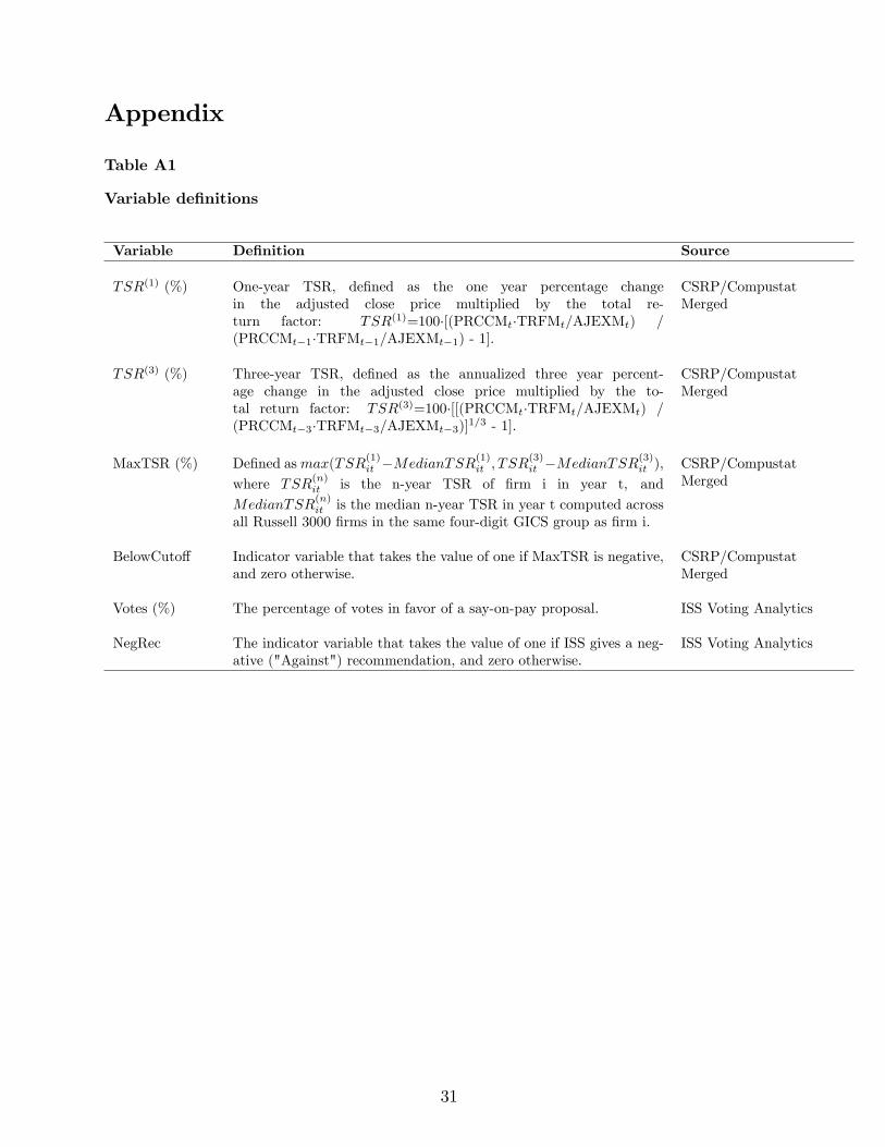
Appendix
Table A1
Variable definitions
Variable Definition Source
T SR(1) (%) One-year TSR, defined as the one year percentage change in the adjusted close price multiplied by the total re-turn factor: T SR(1)=100·[(PRCCMt ·TRFMt/AJEXMt) / (PRCCMt−1 ·TRFMt−1/AJEXMt−1) - 1].
CSRP/Compustat Merged
T SR(3) (%) Three-year TSR, defined as the annualized three year percent-age change in the adjusted close price multiplied by the to-tal return factor: T SR(3)=100·[[(PRCCMt ·TRFMt/AJEXMt) / (PRCCMt−3 ·TRFMt−3/AJEXMt−3)]1/3 - 1].
CSRP/Compustat Merged
MaxTSR (%) (1) (1) (3) (3)Defined as max(T SR −MedianT SR , T SR −MedianT SR ),it it it it (n)where T SR is the n-year TSR of firm i in year t, andit (n)
MedianT SR is the median n-year TSR in year t computed acrossit all Russell 3000 firms in the same four-digit GICS group as firm i.
CSRP/Compustat Merged
BelowCutoff Indicator variable that takes the value of one if MaxTSR is negative, and zero otherwise.
CSRP/Compustat Merged
Votes (%) The percentage of votes in favor of a say-on-pay proposal. ISS Voting Analytics
NegRec The indicator variable that takes the value of one if ISS gives a neg-ative ("Against") recommendation, and zero otherwise.
ISS Voting Analytics
31

Variable Definition Source
Market Value of Equity Market value of equity, which is calculated by multiplying Compustat (in $ billion) the company’s stock price by its number of outstanding
shares as of its fiscal-year-end.
M/B The ratio of the market value of assets (equity market cap- Compustat italization plus the book value of other liabilities) to the book value of assets.
ROA Net income divided by total assets. Compustat
Leverage (Long-term debt + Debt in current liabilities)/Total assets. Compustat
CEO Total Compensation The total compensation of the CEO (variable CEOTotSum- GMI Ratings (in $ million) Comp from GMI Ratings) as reported in the company’s
proxy statement. It equals the aggregate total dollar value of each form of compensation quantified in the summary compensation table, including base salary, bonus, stock awards, option awards, non-equity incentive plan, change in pension value and nonqualified deferred compensation, and all other compensation.
Proportion of Stock-Based The sum of stock and option awards divided by CEO GMI Ratings Compensation total compensation: (CEOOptionAwards + CEOStock-
Awards)/CEOTotSumComp from GMI Ratings.
Growth in CEO Total Defined as (CEO Total Compensation in year t - CEO Total GMI Ratings Compensation Compensation in year t-1)/CEO Total Compensation in
year t-1.
Institutional Ownership Total institutional ownership in fraction of shares outstand- Thomson Reuters 13F ing (Instown_perc from Thomson Reuters 13F).
Institutional Ownership Institutional ownership Herfindahl-Hirschman index, i.e., Thomson Reuters 13F HHI the sum of squared share ownership over all institutional
investors (Instown_HHI from Thomson Reuters 13F).
Insider Ownership The estimated fraction of shares held by top management GMI Ratings and directors, as reported in the firm’s most recent proxy statement (InsidersPctg from GMI Ratings).
Industry dummies Industry fixed effects are based on four-digit GICS classi- Compustat fication to make the definition of the industry consistent with that used by ISS.
32

References
Aggarwal, R., I. Erel, and L. Starks. 2015. Influence of public opinion on investor voting and proxy advisors. Working Paper, Fisher College of Business.
Aghion, P., J. Van Reenen, and L. Zingales. 2013. Innovation and institutional ownership. American Economic Review 103:277—304.
Alexander, C. R., M. A. Chen, D. J. Seppi, and C. S. Spatt. 2010. Interim news and the role of proxy voting advice. Review of Financial Studies 23:4419—54.
Anderson, T. W., and H. Rubin. 1949. Estimation of the parameters of a single equation in a complete system of stochastic equations. Annals of Mathematical Statistics 20:46—63.
Appel, I. R., T. A. Gormley, and D. B. Keim. 2016. Passive investors, not passive owners. Journal of Financial Economics 121:111—41.
Bach, L., and D. Metzger. 2015. Why do shareholder votes matter? Swedish House of Finance Research Paper No. 13-01.
Bethel, J. E., and S. L. Gillan. 2002. The impact of the institutional and regulatory environment on shareholder voting. Financial Management 31:29—54.
Bew, R., and R. Fields. 2012. Voting decisions at US mutual funds: How investors really use proxy advisers. IRRC Institute.
Boone, A. L., and J. T. White. 2015. The effect of institutional ownership on firm transparency and information production. Journal of Financial Economics 117:508—33.
Brav, A., W. Jiang, and H. Kim. 2009. Hedge fund activism: A review. Foundations and Trends in Finance 4:185—246.
Bushee, B., and C. Noe. 2000. Corporate disclosure practices, institutional investors, and stock return volatility. Journal of Accounting Research 38:171—202.
Cai, J., J. L. Garner, and R. A. Walkling. 2009. Electing directors. Journal of Finance 64:2389—421.
Cai, J., and R. A. Walkling. 2011. Shareholders’ say on pay: Does it create value? Journal of Financial and Quantitative Analysis 46:299—339.
Choi, S., J. Fisch, and M. Kahan. 2010. The power of proxy advisors: myth or reality? Emory Law Journal 59:869—918.
Crane, A. D., S. Michenaud, and J. Weston. 2016. The effect of institutional ownership on payout policy: Evidence from index thresholds. Review of Financial Studies 29:1377—408.
Cuñat, V., M. Gine, and M. Guadalupe. 2012. The vote is cast: the effect of corporate governance on shareholder value. Journal of Finance 67:1943—77.
– – – . 2015. Say pays! Shareholder voice and firm performance. Review of Finance. Advance Access published November 28, 2015, 10.1093/rof/rfv056.
Del Guercio, D., L. Seery, and T. Woidtke. 2008. Do boards pay attention when institutional investor activists “just vote no”? Journal of Financial Economics 90:84—103.
Edelman, S. 2013. Proxy advisory firms: a guide for regulatory reform. Emory Law Journal 62:1369— 409.
33

Ertimur, Y., F. Ferri, and V. Muslu. 2011. Shareholder activism and CEO pay. Review of Financial Studies 24:535—92.
Ertimur, Y., F. Ferri, and D. Oesch. 2013. Shareholder votes and proxy advisors: Evidence from say on pay. Journal of Accounting Research 51:951—96.
– – – . 2015. Understanding uncontested director elections: determinants and consequences. Work-ing Paper, Columbia Business School.
Ferri, F. 2012. ‘Low cost’ shareholder activism: A review of the evidence. In Research Handbook on the Economics of Corporate Law. Eds. C. Hill and B. McDonnell. Cheltenham, UK: Elgar Publishers.
Ferri, F., and D. A. Maber. 2013. Say on pay votes and CEO compensation: Evidence from the UK. Review of Finance 17:527—63.
Gallagher, D. M. 2014. Outsized power & influence: The role of proxy advisers. Working Paper Series, Critical Legal Issues.
Gillan, S. L., and L. T. Starks. 2007. The evolution of shareholder activism in the United States. Journal of Applied Corporate Finance 19:55—73.
Hartzell, J. C., and L. T. Starks. 2003. Institutional investors and executive compensation. Journal of Finance 58:2351—74.
Iliev, P., and M. Lowry. 2015. Are mutual funds active voters? Review of Financial Studies 28:446— 85.
Imbens, G. W., and T. Lemieux. 2008. Regression discontinuity designs: A guide to practice. Journal of Econometrics 142:615—35.
Institutional Shareholder Services (ISS). 2012. ISS Responses to ESMA Discussion Paper “An Overview of the Proxy Advisory Industry. Considerations on Possible Policy Options.” Jun 21, 2012.
Karpoff, J. M. 2001. The impact of shareholder activism on target companies: A survey of empirical findings. Working Paper, University of Washington.
Larcker, D. F., A. L. McCall, and G. Ormazabal. 2015. Outsourcing shareholder voting to proxy advisory firms. Journal of Law and Economics 58:173—204.
Levit, D., and N. Malenko. 2011. Nonbinding voting for shareholder proposals. Journal of Finance 66:1579—614.
Malenko, A., and N. Malenko. 2016. Proxy advisory firms: The economics of selling information to voters. Working Paper, MIT.
Matvos, G., and M. Ostrovsky. 2010. Heterogeneity and peer effects in mutual fund proxy voting. Journal of Financial Economics 98:90—112.
McCrary, J. 2008. Manipulation of the running variable in the regression discontinuity design: A density test. Journal of Econometrics 142:698—714.
Morgan, A., A. Poulsen, J. Wolf, and T. Yang. 2011. Mutual funds as monitors: Evidence from mutual fund voting. Journal of Corporate Finance 17:914—28.
Mullins, W. 2014. The governance impact of index funds: Evidence from regression discontinuity.
34

Working Paper, University of Maryland.
Roberts, M. R., and T. M. Whited. 2012. Endogeneity in empirical corporate finance. In Handbook of the Economics of Finance, Volume 2. Eds. G. Constantinides, M. Harris, and R. Stulz. New York City: Elsevier.
Schwartz-Ziv, M., and R. Wermers. 2015. Do small or large shareholders govern their companies through public votes? Evidence from say on pay. Robert H. Smith School Research Paper No. RHS 2510442.
Staiger, D., and J. H. Stock. 1997. Instrumental variables regression with weak instruments. Econo-metrica 65:557—86.
Stock, J. H., J. H. Wright, and M. Yogo. 2002. A survey of weak instruments and weak identification in generalized method of moments. Journal of Business & Economic Statistics 20:518—29.
35

Figures and tables
Figure 1: Probability of a negative ISS recommendation and voting support
(a) (b)
0.1
.2.3
.4
10 8 6 4 2 0 2 4 6 8 10MaxTSR
Probability of a Negative ISS Recommendation
8085
9095
10 8 6 4 2 0 2 4 6 8 10MaxTSR
Percent of Votes in Favor
The figure plots the distribution of negative ISS recommendations and say-on-pay voting support around the cutoff. The x-axis presents the forcing variable MaxT SR, measured in percentage points, in a 10% bandwidth around the cutoff. The y-axis of Figure 1a corresponds to the probability of a negative ISS recommendation, measured in absolute values (from 0 to 1). The y-axis of Figure 1b corresponds to Votes, the percentage of votes in favor of the say-on-pay proposal, measured in percentage points. Each dot in Figure 1a (1b) represents the average probability of a negative ISS recommendation (percentage of votes in favor of the say-on-pay proposal) in bins of 1%. The solid lines represent the fitted values of a third-degree polynomial of MaxT SR estimated on the interval −10% < MaxTSR < 10%.
36

Figure 2: Density of the forcing variable
0.0
5.1
.15
.2
5 0 54 3 2 1 1 2 3 4MaxTSR
Density of MaxTSR
The figure confirms that firms do not manipulate their TSRs to push themselves above the cutoff by showing that the density of the forcing variable is continuous. The x-axis presents the forcing variable MaxT SR, measured in percentage points, in a 5% bandwidth around the cutoff. The y-axis corresponds to the density of MaxT SR, measured in absolute values. The figure shows the histogram, estimated density, and 95% confidence intervals of MaxT SR in a 5% bandwidth. The absolute value of the McCrary (2008) test statistic is 0.84, which is not statistically significantly different from zero at any conventional level. Both the figure and the McCrary test statistic were generated using the code provided by J. McCrary on his website: http://eml.berkeley.edu/~jmccrary/DCdensity/.
37

Figure 3: Falsification tests on alternative samples
(a) Say-on-pay proposals in 2012 (b) Director elections in 2010-2011
8085
9095
100
5 4 3 2 1 0 1 2 3 4 5MaxTSR
Percent of Votes in Favor
9092
9496
98
5 4 3 2 1 0 1 2 3 4 5MaxTSR
Percent of Votes in Favor
(c) Compensation committee elections in 2010-2011 (d) Director elections in 2012
8590
9510
0
5 4 3 2 1 0 1 2 3 4 5MaxTSR
Percent of Votes in Favor85
9095
100
5 4 3 2 1 0 1 2 3 4 5MaxTSR
Percent of Votes in Favor
The figure shows that voting support is continuous for samples where the cutoff rule does not apply. Figure 3a considers say-on-pay proposals in 2012. Figure 3b considers director elections in 2010-2011, where to match our main sample, we restrict attention to those firms in each year that had a say-on-pay vote in that year. Figure 3c restricts the sample in Figure 3b to the elections of compensation committee members. Figure 3d considers director elections in 2012. Because each firm has many directors but only one say-on-pay proposal, we aggregate director election observations by firm-year-recommendation to make the sample consistent with our main sample: for each firm-year, we calculate the average voting support for all directors who received a positive (negative) recommendation. Samples a-d have 289, 470, 263, and 332 observations, respectively.
38

Table 1: Descriptive statistics
Panel A Full sample 5% bandwidth Diff. in
means Mean 25th 50th 75th SD Mean 25th 50th 75th SD p-val
Market Value of Equity 5.53 0.44 1.15 3.50 17.78 7.97 0.64 1.64 4.37 26.47 0.08
ROA 0.02 0.00 0.03 0.07 0.15 0.03 0.01 0.03 0.07 0.12 0.19
Leverage 0.20 0.04 0.16 0.31 0.20 0.22 0.06 0.18 0.32 0.19 0.15
Market-to-Book 1.90 1.04 1.35 2.06 1.68 1.59 1.02 1.26 1.78 0.92 0.00
Institutional Ownership 0.72 0.58 0.76 0.89 0.23 0.71 0.57 0.75 0.88 0.22 0.65
Inst. Ownership HHI 0.06 0.04 0.05 0.07 0.06 0.06 0.04 0.05 0.06 0.07 0.62
CEO Total Comp. 4.76 1.46 3.00 6.20 4.96 5.44 1.73 3.64 6.93 5.17 0.01
% of Stock-Based Comp. 0.40 0.23 0.42 0.57 0.27 0.42 0.27 0.45 0.57 0.23 0.29
Growth in CEO Comp. 0.47 -0.07 0.18 0.59 1.62 0.42 -0.10 0.12 0.48 1.55 0.58
Panel B Number of observations
Voting support by voting outcome
ISS recommendation Mean 10th 50th 90th SD Fail Pass Total
Against 68.9% 48.5% 68.9% 88.7% 15.2% 29 227 256
For 93.2% 83.3% 95.6% 99.1% 7.0% 0 1,764 1,764
Total (Against and For) 90.1% 73.5% 94.9% 99.0% 11.7% 29 1,991 2,020
Panel A presents the summary statistics of the variables used in the study for the full sample of 2,020 say-on-pay proposals in 2010-2011 and for the 404 observations in the 5% bandwidth around the cutoff. The last column in Panel A shows the p-values for the difference in means test between the full sample and the 5% bandwidth. Panel B presents the distribution of voting support and the number of fail vs. pass voting outcomes depending on the ISS recommendation, where a proposal fails if it receives less than 50% support. The last column presents the total number of observations with a given ISS recommendation. Variable definitions are provided in the appendix.
39

Table 2: Probability of a negative ISS recommendation (first stage) (1) (2) (3) (4) (5)
NegRec NegRec NegRec NegRec NegRec
BelowCutoff 0.145** 0.146** 0.146** 0.148** 0.142**
(0.068) (0.069) (0.070) (0.067) (0.067)
MaxTSR -0.008 -0.010 -0.017 -0.012 -0.014
(0.012) (0.016) (0.016) (0.016) (0.016)
BelowCutoff·MaxTSR 0.004 0.013 0.009 0.010
(0.024) (0.024) (0.023) (0.023)
CEO Total Compensation 0.007* 0.018***
(0.004) (0.006)
Growth in CEO Total Compensation 0.062*** 0.061***
(0.012) (0.012)
Proportion of Stock-Based Compensation -0.064 -0.060
(0.093) (0.095)
Institutional Ownership -0.007 0.004
(0.096) (0.096)
Insider Ownership 0.412*** 0.360***
(0.125) (0.127)
Log(Market Value of Equity) -0.043**
(0.020)
ROA -0.133
(0.172)
M/B 0.024
(0.023)
Year FE No No Yes Yes Yes
Industry FE No No Yes Yes Yes
Observations 403 403 403 394 393
R2 0.062 0.062 0.076 0.184 0.198
F-statistic 4.49 4.52 4.33 4.85 4.45
The table presents the first-stage estimates and shows that the probability of a negative ISS recom-mendation increases discontinuously for firms below the ISS cutoff. All specifications are estimated on a 5% bandwidth. The outcome variable is NegRec, which equals one if ISS gives a negative recom-mendation, and zero otherwise. The main variable of interest is BelowCutoff , which equals one if the firm is below the cutoff (MaxT SR < 0), and zero otherwise. We estimate a linear probability model, and hence the coeffi cient on BelowCutoff measures the difference in the probability of a negative recommendation between firms just below and just above the cutoff. Standard errors are reported in parentheses. *, **, and *** represent significance at the 10%, 5%, and 1% levels, respectively.
40

Table 3: Effect of ISS recommendations on voting outcomes (second stage)
(1) (2) (3) (4) (5)
Votes Votes Votes Votes Votes
NegRec -24.620** -25.111** -29.001** -28.717*** -26.555**
(11.210) (11.160) (11.588) (10.655) (10.853)
MaxTSR 0.045 0.175 0.129 0.125 0.226
(0.358) (0.450) (0.531) (0.455) (0.463)
BelowCutoff·MaxTSR -0.294 -0.302 -0.198 -0.277
(0.560) (0.585) (0.544) (0.534)
CEO Total Compensation -0.273** -0.677***
(0.120) (0.241)
Growth in CEO Total Compensation 0.261 0.167
(0.720) (0.717)
Proportion of Stock-Based Compensation -0.047 -0.210
(2.228) (2.218)
Institutional Ownership -5.597** -6.009***
(2.246) (2.186)
Insider Ownership 13.023** 14.370***
(5.292) (4.861)
Log(Market Value of Equity) 1.658**
(0.665)
ROA 5.750
(4.247)
M/B 0.353
(0.585)
Year FE No No Yes Yes Yes
Industry FE No No Yes Yes Yes
Observations 403 403 403 394 393
R2 0.547 0.547 0.536 0.605 0.628
OLS coeffi cient on NegRec -25.339*** -25.338*** -25.052*** -26.070*** -25.443***
(1.185) (1.186) (1.227) (1.234) (1.222)
Durbin-Wu-Hausman test p-value 0.949 0.984 0.720 0.795 0.915
The table shows that a negative ISS recommendation causes a significant decline in say-on-pay voting support. The outcome variable is Votes, the percentage of votes in favor of a say-on-pay proposal, measured in percentage points. The main explanatory variable is NegRec, which equals one if ISS gives a negative recommendation, and zero otherwise. Estimation is conducted via 2SLS, where NegRec is the instrumented variable, the first stage is estimated in Table 2, and the second stage is estimated in this table. The last three rows present the coeffi cient and standard error on NegRec in the OLS regression of Votes on NegRec with the same set of regressors as in the corresponding 2SLS regression, and the p-value of the Durbin-Wu-Hausman test for equality of the OLS and IV estimates. All specifications are estimated on a 5% bandwidth. Standard errors are reported in parentheses. *, **, and *** represent significance at the 10%, 5%, and 1% levels, respectively.
41

Table 4: Variation in the effect of ISS across firms
42
BelowCutoff
(First Stage)
(1)
Inst.Ownership HHI
Low High
0.164** 0.158**
(0.071) (0.066)
(2)
% Inst.Blockholders
Low High
0.126* 0.169**
(0.070) (0.073)
(3)
% Top 10 Institutions
Low High
0.163** 0.156**
(0.070) (0.066)
(4)
% Passive Institutions
Low High
0.201*** 0.159**
(0.070) (0.066)
(5)
Inst.Ownership
Low High
0.176** 0.187***
(0.068) (0.069)
NegRec
(Second Stage)
-41.12***
(12.07)
-21.27*
(11.04)
-35.72**
(16.33)
-25.56**
(11.95)
-37.48***
(11.20)
-23.38**
(11.21)
-18.87**
(7.78)
-38.20***
(11.76)
-24.08***
(8.65)
-32.30***
(10.19)
MaxTSR controls
Year FE
Industry FE
Observations
Yes
Yes
Yes
386
Yes
Yes
Yes
386
Yes
Yes
Yes
337
Yes
Yes
Yes
336
Yes
Yes
Yes
385
Yes
Yes
Yes
387
Yes
Yes
Yes
384
Yes
Yes
Yes
384
Yes
Yes
Yes
388
Yes
Yes
Yes
389
The table shows how the effect of ISS varies with the firm’s ownership structure. Inst.Ownership HHI is the Herfindahl-Hirschman index, defined as the sum of squared share ownership over all institutional investors. % Inst.Blockholders is the percent of institutional shares held by blockholders, defined as the ratio of total ownership by institutional blockholders to total institutional ownership (instblockown/instown from Thomson Reuters). % Top 10 Institutions is the percent of institutional shares held by the top 10 largest institutions, defined as the ratio of ownership by the top 10 institutional investors to total institutional ownership (top10instown/instown from Thomson Reuters). % Passive Institutions is the percent of shares held by “transient”and “quasi-index”institutional investors in the classification of Bushee and Noe (2000). Inst.Ownership is total institutional ownership in fraction of shares outstanding. For each ownership characteristic, we first restrict the sample to observations with MaxT SR within a 10% bandwidth and calculate the median value of the ownership characteristic in the resulting sample. Next, we divide this sample into two subsamples, based on whether the corresponding ownership characteristic falls below or above the median, and refer to the first and second subsample as the “Low”and “High” subsample, respectively. We then repeat the 2SLS procedure on each of the two subsamples. Each specification controls for MaxT SR, BelowCutoff ·MaxT SR, and year and industry fixed effects. *, **, and *** represent significance at the 10%, 5%, and 1% levels, respectively.

43
Table 5: Robustness
(1) (2) (3) (4) (5) (6) (7) (8) (9) (10) (11)
3% 4% 5% 6% 7% 8% 9% 10% 20% Quadratic
20% Cubic
20% Quartic
BelowCutoff 0.18** 0.17** 0.15** 0.19*** 0.19*** 0.19*** 0.20*** 0.18*** 0.19*** 0.19*** 0.21***
(0.09) (0.08) (0.07) (0.06) (0.06) (0.05) (0.05) (0.05) (0.05) (0.07) (0.08)
NegRec -20.33* -24.68** -29.00** -27.99*** -21.09*** -23.47*** -23.29*** -28.56*** -22.38*** -23.62*** -23.91**
(12.01) (10.26) (11.59) (8.33) (7.81) (7.08) (6.37) (6.93) (7.07) (9.16) (10.18)
Observations 238 313 403 490 574 651 717 785 1,244 1,244 1,244
The table shows robustness to the choice of the bandwidth and the degree of the polynomial. The first two rows present the estimate and standard error of the coeffi cient on BelowCutoff in the first-stage regression. The third and fourth rows present the estimate and standard error of the coeffi cient on NegRec in the second-stage regression. Columns 1-8 present the linear specification on bandwidths between 3% and 10%. Columns 9-11 present the estimation of the second, third, and fourth-order polynomial functions of MaxT SR on a 20% bandwidth, allowing for different functional forms around the cutoff. All specifications control for year and industry fixed effects. For example, the regressors in column 9 include BelowCutoff , MaxT SR, MaxT SR2 , BelowCutoff ·MaxT SR, BelowCutoff ·MaxT SR2 , and year and industry fixed effects. *, **, and *** represent significance at the 10%, 5%, and 1% levels, respectively.

Table 6: Distribution of firm characteristics around the cutoff
RD coeff. on (-5%, 0) (0, 5%) Diff. in means
BelowCutoff Mean Obs Mean Obs p-val
Log(Market Value of Equity) -0.02
(0.29) 0.71 173 0.58 230 0.39
M/B -0.10
(0.15) 1.56 173 1.62 229 0.49
ROA -0.03
(0.02) 0.03 173 0.03 230 0.82
Leverage 0.00
(0.04) 0.21 165 0.22 216 0.74
CEO Total Compensation 0.06
(0.96) 5.81 173 5.17 230 0.22
CEO Compensation Percentile 1.29
(5.21) 60.3 173 57.9 230 0.38
Proportion of Stock-Based Compensation 0.06
(0.04) 0.42 173 0.42 230 0.91
Proportion of Incentive Pay 0.02
(0.05) 0.53 170 0.55 226 0.51
1-year growth in CEO Total Compensation 0.06
(0.29) 0.44 172 0.41 227 0.85
3-year growth in CEO Total Compensation -0.03
(0.04) 0.05 154 0.05 207 0.91
Institutional Ownership -0.03
(0.04) 0.72 173 0.71 230 0.62
Insider Ownership 0.01
(0.03) 0.12 169 0.09 226 0.12
The table shows that the distribution of firm characteristics is smooth around the cutoff. For each characteristic in the first column, column “RD coeff. on BelowCutoff” presents the results of a local linear regression of this characteristic on BelowCutoff , MaxT SR, BelowCutoff ·MaxT SR, and year and industry fixed effects using a 5% bandwidth. The estimated coeffi cients on BelowCutoff are reported in the first row, and standard errors are reported in parentheses. Subsequent columns present the means of each characteristic in two intervals: −5% < MaxTSR < 0 and 0 < MaxTSR < 5%, as well as the number of observations in these intervals. The last column presents the p-values for the difference in means test. CEO Compensation Percentile is the percentile of CEO Total Compensation in the firm’s four-digit GICS group in that year. Proportion of Incentive Pay is the proportion of total compensation represented by incentive pay (variable CEOVariableTPM from GMI Ratings). 3-year growth in CEO Total Compensation is defined as (CEO Total Compensationt − CEO Total Compensationt−3)/CEO Total Compensationt. Other variable definitions are provided in the appendix.
44

Table 7: Instrument strength
5% 6% 7% 8% 9% 10%
First-stage F-statistic 4.33 8.55 10.46 12.71 16.06 14.32
Anderson-Rubin p-value 0.086 0.018 0.055 0.018 0.009 0.003
Reduced form regression -4.22*
(2.42)
-5.20**
(2.17)
-3.91**
(1.99)
-4.45**
(1.84)
-4.63***
(1.74)
-5.07***
(1.65)
Observations 403 490 574 651 717 785
The first row presents the first-stage F-statistic for bandwidths ranging between 5% and 10%. The second row presents the p-value of the Anderson-Rubin statistic for the second-stage coeffi cient on NegRec, which is obtained using the Stata package condivreg. The third and fourth rows present the estimate and standard error of the coeffi cient on BelowCutoff in the reduced form regression of Votes on BelowCutoff . In all the tests and for all bandwidths, we control for MaxT SR, BelowCut-off ·MaxT SR, and year and industry fixed effects. *, **, and *** represent significance at the 10%, 5%, and 1% levels, respectively.
45