Oct. 6, 2010 1

Lecture 9

Population Ecology

Oct. 6, 2010 2

Today’s topics

• What is population ecology?• Population change and regulation

– Density independence– Density dependence

• Life history traits• Alaska example

– Predator control

Oct. 6, 2010 3

Population-groups of organisms of the same species, present at the same place and time

• Population ecologists are often concerned with population dynamics: the changes that occur over time and what causes those changes.

Oct. 6, 2010 4

Population ecology questions…

• What is the the size of the population?– Census – try to count every individual– Estimate – survey a portion of the population and

extrapolate.

Oct. 6, 2010 5

Caribou census – aerial photographs

Oct. 6, 2010 6

Moose estimate – aerial surveys

Oct. 6, 2010 7

Deer estimate - DNA

Oct. 6, 2010 8

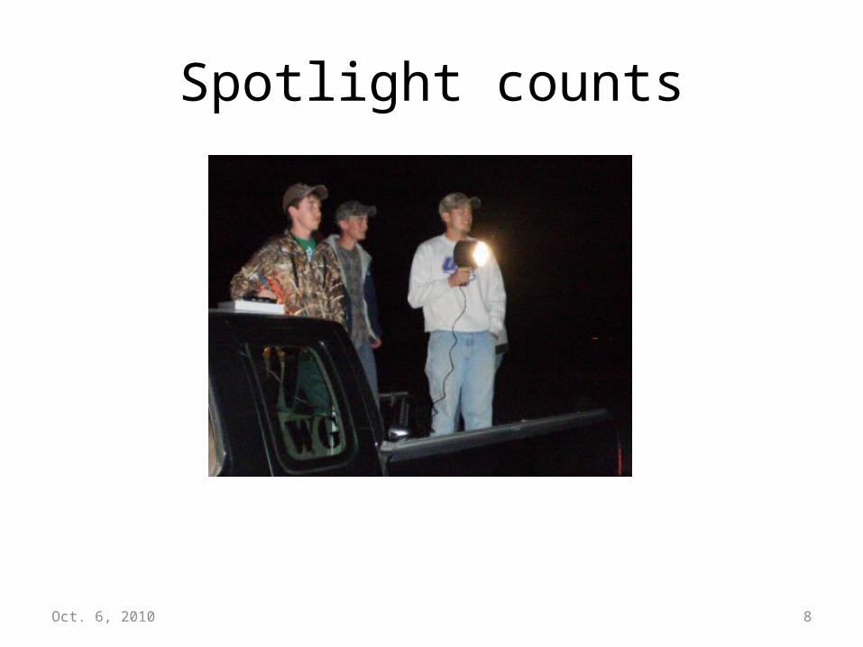
Spotlight counts

Oct. 6, 2010 9

Population ecology questions…

• Is the population increasing or decreasing?– Birth rates – individuals added per unit time– Death rates – individuals deleted per unit time– Immigration rates – individual moving in per unit

time– Emigration rates – individuals moving out per unit

time

Oct. 6, 2010 10

Not all individual are identical• For instance, birth rates, death rates, and

movement rates depend on age, sex, and many other characteristics of an individual and the environment.

Oct. 6, 2010 11

Senescence – decrease in fecundity and increase in mortality rate resulting from deterioration

in physiological function with age.

Age

Offspring per individual female

Oct. 6, 2010 12

Life tables – summary by age of survivorship of an individual in a population (simple version)

• Need to know how many are dying in each age interval.

• For example:

Age interval, years, x Number dying, dx

0-1 10

1-2 6

2-3 2

3-4 1

Oct. 6, 2010 13

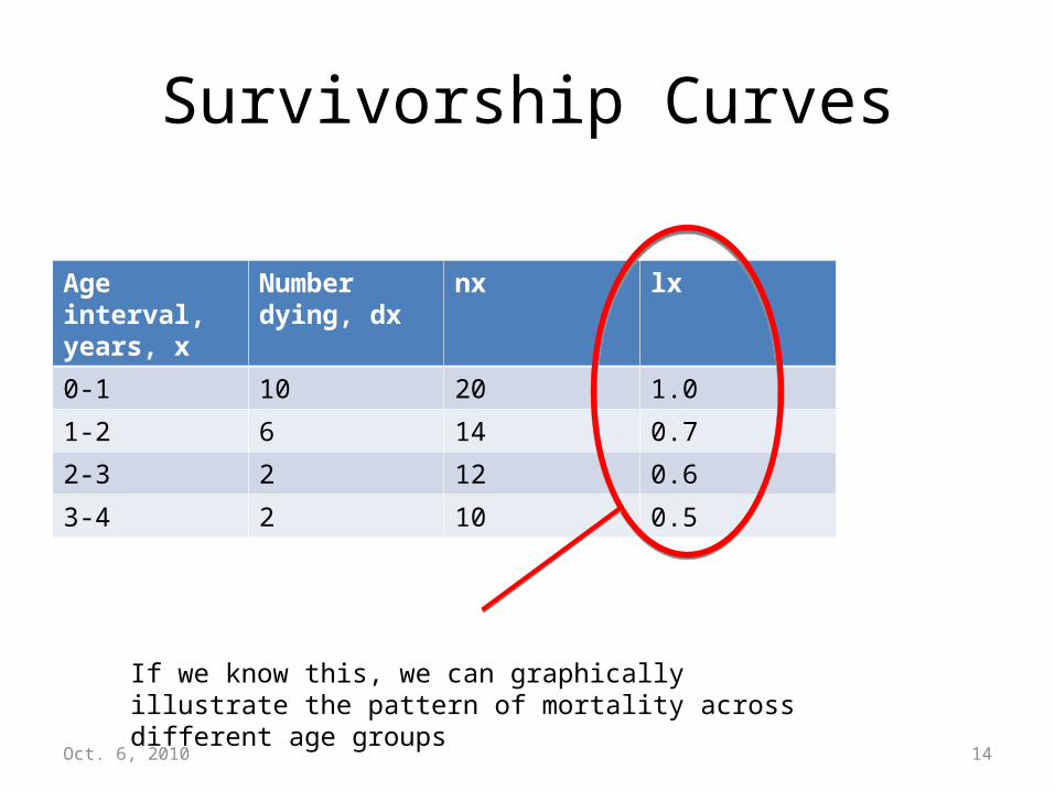
From there, we can compute number surviving (nx) and cumulative survival

rate from birth until age x (lx)

Age interval, years, x

Number dying, dx

nx lx

0-1 10 20 1.0

1-2 6 14 0.7

2-3 2 12 0.6

3-4 2 10 0.5

Oct. 6, 2010 14

Survivorship Curves

Age interval, years, x

Number dying, dx

nx lx

0-1 10 20 1.0

1-2 6 14 0.7

2-3 2 12 0.6

3-4 2 10 0.5

If we know this, we can graphically illustrate the pattern of mortality across different age groups

Oct. 6, 2010 15

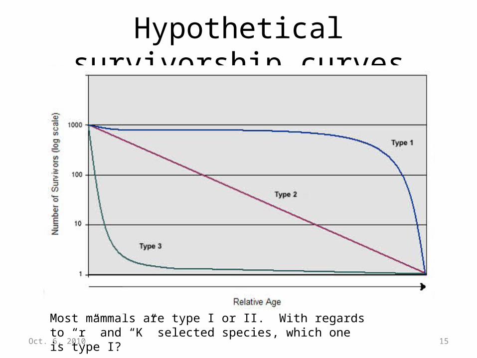
Hypothetical survivorship curves

Most mammals are type I or II. With regards to “r” and “K” selected species, which one is type I?

Oct. 6, 2010 16

More complex life tables

• Fecundity (mx) = number of offspring produced by an average female of age x during that age period

• Survival rate (sx) = survival rate at age x• Mortality rate (qx) = mortality rate at age x

Oct. 6, 2010 17

If we know change over time, then we can compute λ (lamda)

• λ = population growth rate from one point in time (t) to some future time (t + 1)

• For example, if there is 100 individuals in the population one year ago and there is 110 now, then..

N(t+1) = λN(t)

110 = λ100

λ = 1.1

λ sometimes called finite rate of population increase

Oct. 6, 2010 18

Assuming λ is constant over time

• How much will the population grow in 10 years?

Nt = λtN0

Nt = 1.110*100

Nt = ?

Important note = this equation assumes unimpeded growth (no density dependence factors operating on population)

Oct. 6, 2010 19

Populations increase exponentially rather than arithmetically

Oct. 6, 2010 20

Density Dependence• It is impossible for an population to continue

to grow indefinitely at a constant rate.• Growth will slow as limiting factors exert

influence– Food supply– Shelter– Predators– Competitors– Parasites– Disease

• The influence often increases as the size and density of the population increases

Oct. 6, 2010 21

With density dependence

• As density increases, birth rates decrease, death rates increase, and/or emigration increases

• The logistic curve represents population change over time in a density dependent system.

• “K” plays a key role the logistic curve model.

Oct. 6, 2010 22

Logistic curve

Oct. 6, 2010 23

Logistic Equation

dN

dtrN 1

N

K

dN/dt = Population growth rateK = carrying capacity of the populationr = growth rate per individual or intrinsic rate of natural increase“r” can be calculated as individual birth rate minus individual death rate

Oct. 6, 2010 24

Logistic Equation

dN

dtrN 1

N

K

The term in parenthesis is a density dependent term that ranges from 0 to 1.

As N approaches K, then the density dependent term approaches 0.

As the density dependent term approaches 0, the growth rate slows.

Oct. 6, 2010 25

Logistic Equation

dN

dtrN 1

N

K

Simply, as the size of a mammal population approaches the maximum number that the habitat can support, the growth rate of the population slows..

Oct. 6, 2010 26

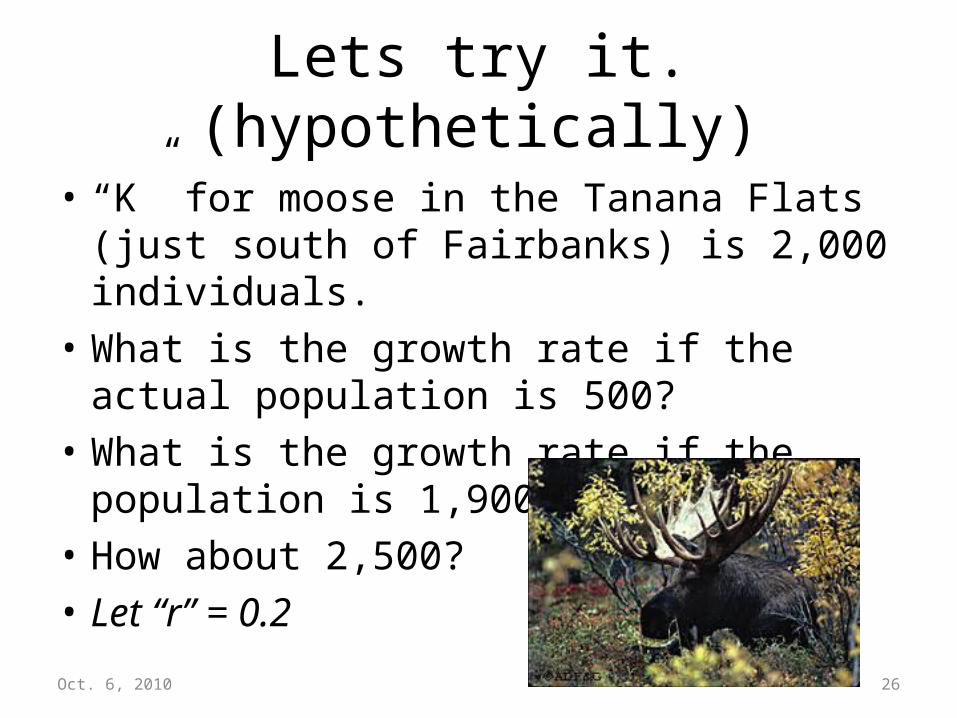
Lets try it. (hypothetically)

• “K” for moose in the Tanana Flats (just south of Fairbanks) is 2,000 individuals.

• What is the growth rate if the actual population is 500?

• What is the growth rate if the population is 1,900?

• How about 2,500?• Let “r” = 0.2

Oct. 6, 2010 27

Oct. 6, 2010 28

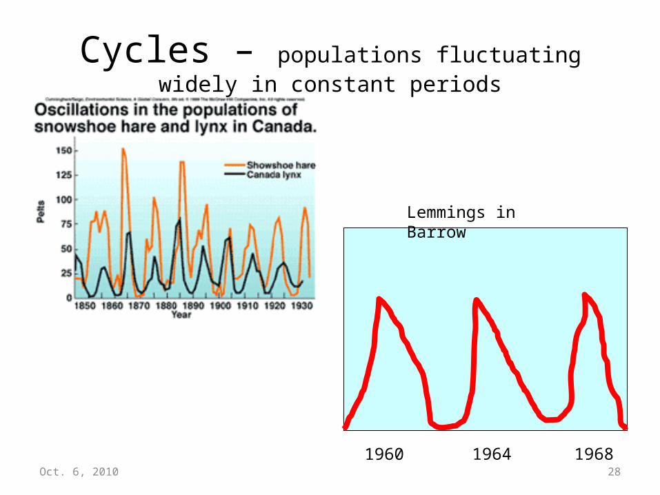
Cycles – populations fluctuating widely in constant periods

1960 1964 1968

Lemmings in Barrow

Oct. 6, 2010 29

Alaska Example• Intensive Management (i.e., predator control)

Oct. 6, 2010 30

Increase in moose, caribou, and wolves following wolf control in Alaska (Boertje et al. 1996)

14 wolves/1,000 km2Before 1975

1975

1975-1982 4-5 wolves/1,000 km2

Predator control for 7 years

1982Stop predator control

1986 15-16 wolves/1,000 km2

Oct. 6, 2010 31

How did moose respond183 moose/1,000 km2Before 1975

1975

1975-1982 481 moose/1,000 km2

Predator control for 7 years

1982Stop predator control

λ = 1.15

1982-1994 λ = 1.051,020 moose/1,000 km2

Oct. 6, 2010 32

Why did killing wolves increase the wolf population?

Why did the moose population continue to increase after the wolf

population recovered?

Oct. 6, 2010 33

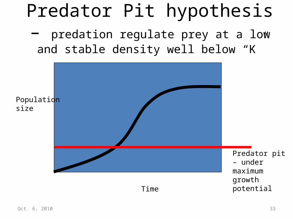
Predator Pit hypothesis – predation regulate prey at a low and stable density well below “K”

Time

Population size

Predator pit – under maximum growth potential

Oct. 6, 2010 34

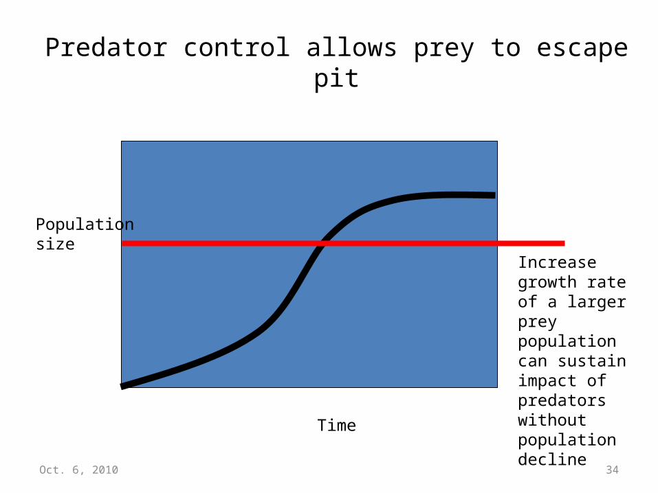
Predator control allows prey to escape pit

Time

Population size

Increase growth rate of a larger prey population can sustain impact of predators without population decline

Oct. 6, 2010 35

Danger! Knowing “K” is important

Time

Population size

K

Unsustainable level

Oct. 6, 2010 36

Elevating prey base above “K” may result in habitat damage, crash the population, and potential reduce

future “K”.

Time

K

Pop

Time

K

Time

KPop

Pop

Oct. 6, 2010 37

The story gets even more ecologically complex and political.

• Maybe a report topic???