![From Lattice Boltzmann Method to Lattice Boltzmann Flux … · From Lattice Boltzmann Method to Lattice Boltzmann Flux Solver Yan Wang 1, ... flows [8,13–15], compressible flows](https://static.fdocuments.in/doc/165x107/5cadf91b88c9938f4d8c0cd6/from-lattice-boltzmann-method-to-lattice-boltzmann-flux-from-lattice-boltzmann.jpg)
Ocneanu cells and Boltzmann weights for ... - uni … · Ocneanu cells and Boltzmann weights for...
48
M¨ unster J. of Math. 2 (2009), 95–142 M¨ unster Journal of Mathematics urn:nbn:de:hbz:6-10569512950 c M¨ unster J. of Math. 2009 Ocneanu cells and Boltzmann weights for the SU (3) ADE graphs David E. Evans and Mathew Pugh (Communicated by Siegfried Echterhoff) Dedicated to Joachim Cuntz on the occasion of his 60th birthday Abstract. We determine the cells, whose existence has been announced by Ocneanu, on all the candidate nimrep graphs except E (12) 4 proposed by di Francesco and Zuber for the SU (3) modular invariants classified by Gannon. This enables the Boltzmann weights to be computed for the corresponding integrable statistical mechanical models and provide the framework for studying corresponding braided subfactors to realize all the SU (3) modular invariants as well as a framework for a new SU (3) planar algebra theory. 1. Introduction In the last twenty years, a very fruitful circle of ideas has developed link- ing the theory of subfactors with modular invariants in conformal field theory. Subfactors have been studied through their paragroups, planar algebras and have serious contact with free probability theory. The understanding and clas- sification of modular invariants is significant for conformal field theory and their underlying statistical mechanical models. These areas are linked through the use of braided subfactors and α-induction which in particular for SU (2) subfactors and SU (2) modular invariants invokes ADE classifications on both sides. This paper is the first of our series to study more precisely these con- nections in the context of SU (3) subfactors and SU (3) modular invariants. The aim is to understand them not only through braided subfactors and α- induction but introduce and develop a pertinent planar algebra theory and free probability. A group acting on a factor can be recovered from the inclusion of its fixed point algebra. A general subfactor encodes a more sophisticated symmetry or a way of handling non group like symmetries including but going beyond quan- tum groups [18]. The classification of subfactors was initiated by Jones [29]
Transcript of Ocneanu cells and Boltzmann weights for ... - uni … · Ocneanu cells and Boltzmann weights for...

Munster J. of Math. 2 (2009), 95–142 Munster Journal of Mathematics
urn:nbn:de:hbz:6-10569512950 c© Munster J. of Math. 2009
Ocneanu cells and Boltzmann weights for the
SU(3) ADE graphs
David E. Evans and Mathew Pugh
(Communicated by Siegfried Echterhoff)
Dedicated to Joachim Cuntz on the occasion of his 60th birthday
Abstract. We determine the cells, whose existence has been announced by Ocneanu, on
all the candidate nimrep graphs except E(12)4 proposed by di Francesco and Zuber for the
SU(3) modular invariants classified by Gannon. This enables the Boltzmann weights to becomputed for the corresponding integrable statistical mechanical models and provide theframework for studying corresponding braided subfactors to realize all the SU(3) modularinvariants as well as a framework for a new SU(3) planar algebra theory.
1. Introduction
In the last twenty years, a very fruitful circle of ideas has developed link-ing the theory of subfactors with modular invariants in conformal field theory.Subfactors have been studied through their paragroups, planar algebras andhave serious contact with free probability theory. The understanding and clas-sification of modular invariants is significant for conformal field theory andtheir underlying statistical mechanical models. These areas are linked throughthe use of braided subfactors and α-induction which in particular for SU(2)subfactors and SU(2) modular invariants invokes ADE classifications on bothsides. This paper is the first of our series to study more precisely these con-nections in the context of SU(3) subfactors and SU(3) modular invariants.The aim is to understand them not only through braided subfactors and α-induction but introduce and develop a pertinent planar algebra theory and freeprobability.
A group acting on a factor can be recovered from the inclusion of its fixedpoint algebra. A general subfactor encodes a more sophisticated symmetry ora way of handling non group like symmetries including but going beyond quan-tum groups [18]. The classification of subfactors was initiated by Jones [29]

96 David E. Evans and Mathew Pugh
who found that the minimal symmetry to understand the inclusion is throughthe Temperley-Lieb algebra. This arises from the representation theory ofSU(2) or dually certain representations of Hecke algebras. All SU(2) modularinvariant partition functions were classified by Cappelli, Itzykson and Zuber[11, 12] using ADE Coxeter-Dynkin diagrams and their realization by braidedsubfactors is reviewed and referenced in [15]. There are a number of invari-ants (encoding the symmetry) one can assign to a subfactor, and under certaincircumstances they are complete at least for hyperfinite subfactors. Popa [39]axiomatized the inclusions of relative commutants in the Jones tower, andJones [30] showed that this was equivalent to his planar algebra description.Here one is naturally forced to work with nonamenable factors through freeprobabilistic constructions e.g. [27]. In another vein, Banica and Bisch [3]understood the principal graphs, which encode only the multiplicities in theinclusions of the relative commutants, and more generally nimrep graphs interms of spectral measures, and so provide another way of understanding thesubfactor invariants.
In our series of papers we will look at this in the context of SU(3), throughthe subfactor theory and their modular invariants, beginning here and contin-uing in [20, 21, 22, 23, 24]. The SU(3) modular invariants were classified byGannon [26]. Ocneanu [37] announced that all these modular invariants wererealized by subfactors, and most of these are understood in the literature andwill be reviewed in the sequel [20]. A braided subfactor automatically givesa modular invariant through α-induction. This α-induction yields a represen-tation of the Verlinde algebra or a nimrep - which yields multiplicity graphsassociated to the modular invariants (or at least associated to the inclusion,as a modular invariant may be represented by wildly differing inclusions andso may possess inequivalent but isospectral nimreps, as is the case for E(12)).In the case of the SU(3) modular invariants, candidates of these graphs wereproposed by di Francesco and Zuber [14] by looking for graphs whose spectrumreproduced the diagonal part of the modular invariant, aided to some degreeby first listing the graphs and spectra of fusion graphs of the finite subgroupsof SU(3). In the SU(2) situation there is a precise relation between the ADECoxeter-Dynkin graphs and finite subgroups of SU(2) as part of the McKaycorrespondence. However, for SU(3), the relation between nimrep graphs andfinite subgroups of SU(3) is imprecise and not a perfect match. For SU(2), anaffine Dynkin diagram describing the McKay graph of a finite subgroup givesrise to a Dynkin diagram describing a nimrep or the diagonal part of a modularinvariant by removing the vertex corresponding to the identity representation.Di Francesco and Zuber found graphs whose spectrum described the diagonalpart of a modular invariant by taking the list of McKay graphs of finite sub-groups of SU(3) and removing vertices. Not every modular invariant couldbe described in this way, and not every finite subgroup yielded a nimrep for amodular invariant. In higher rank SU(N), the number of finite subgroups willincrease but the number of exceptional modular invariants should decrease, so
Munster Journal of Mathematics Vol. 2 (2009), 95–142

Ocneanu cells and Boltzmann weights for SU(3) ADE graphs 97
this procedure is even less likely to be accurate. Evans and Gannon have sug-gested an alternative way of associating finite subgroups to modular invariants,by considering the largest finite stabilizer groups [16].
A modular invariant which is realized by a subfactor will yield a graph. Toconstruct these subfactors we will need some input graphs which will actu-ally coincide with the output nimrep graphs - SU(3) ADE graphs. The aimof this series of papers is to study the SU(3) ADE graphs, which appear inthe classification of modular invariant partition functions from numerous view-points including the determination of their Boltzmann weights in this paper,representations of SU(3)-Temperley-Lieb or Hecke algebra [20], a new notionof SU(3)-planar algebras [21] and their modules [22], and spectral measures[23, 24].
As pointed out to us by Jean-Bernard Zuber, there is a renewal of interest(by physicists) in these SU(3) and related theories, in connection with topo-logical quantum computing [1] and by Joost Slingerland in connection withcondensed matter physics [2] where we see that α-induction is playing a keyrole.
We begin however in this paper by computing the numerical values of theOcneanu cells, and consequently representations of the Hecke algebra, for theADE graphs. These cells give numerical weight to Kuperberg’s [32] diagramof trivalent vertices—corresponding to the fact that the trivial representationis contained in the triple product of the fundamental representation of SU(3)through the determinant. They will yield in a natural way, representations ofan SU(3)-Temperley-Lieb or Hecke algebra. (For SU(2) or bipartite graphs,the corresponding weights (associated to the diagrams of cups or caps), arisein a more straightforward fashion from a Perron-Frobenius eigenvector, givinga natural representation of the Temperley-Lieb algebra or Hecke algebra). We
have been unable thus far to compute the cells for the exceptional graph E(12)4 .
This graph is meant to be the nimrep for the modular invariant conjugate to
the Moore-Seiberg invariant E(12)MS [33]. However we will still be able to realize
this modular invariant by subfactors in [20] using [19]. For the orbifold graphs
D(3k), k = 2, 3, . . . , orbifold conjugate D(n)∗, n = 6, 7, . . . , and E(12)1 we
compute solutions which satisfy some additional condition, but for the othergraphs we compute all the Ocneanu cells, up to equivalence. The existenceof these cells has been announced by Ocneanu (e.g. [36, 37]), although thenumerical values have remained unpublished. Some of the representations ofthe Hecke algebra have appeared in the literature and we compare our results.
For the A graphs, our solution for the Ocneanu cells W gives an identicalrepresentation of the Hecke algebra to that of Jimbo et al. [28] given in (21).Our cells for the A(n)∗ graphs give equivalent Boltzmann weights to thosegiven by Behrend and Evans in [4]. In [14], di Francesco and Zuber give arepresentation of the Hecke algebra for the graphs D(6)∗ and E(8), whilst in
[41] a representation of the Hecke algebra is computed for the graphs E(12)1 and
E(24). Our solutions for the cells W give an identical Hecke representation for
Munster Journal of Mathematics Vol. 2 (2009), 95–142

98 David E. Evans and Mathew Pugh
E(8) and an equivalent Hecke representation for E(12)1 . However, for E(24), our
cells give inequivalent Boltzmann weights. In [25], Fendley gives Boltzmannweights for D(6) which are not equivalent to those we obtain, but which areequivalent if we take one of the weights in [25] to be the complex conjugate ofwhat is given.
Subsequently, we will use these weights, their existence and occasionallymore precise use of their numerical values. Here we outline some of the flavorof these applications. We use these cells to define an SU(3) analogue of theGoodman-de la Harpe Jones construction of a subfactor, where we embedthe SU(3)-Temperley-Lieb or Hecke algebra in an AF path algebra of theSU(3) ADE graphs. Using this construction, we realize all the SU(3) modularinvariants by subfactors [20].
We will then [21, 22] look at the SU(3)-Temperley-Lieb algebra and theSU(3)-GHJ subfactors from the viewpoint of planar algebras. We give a di-agrammatic representation of the SU(3)-Temperley-Lieb algebra, and showthat it is isomorphic to Wenzl’s representation of a Hecke algebra. Generaliz-ing Jones’s notion of a planar algebra, we construct an SU(3)-planar algebrawhich will capture the structure contained in the SU(3) ADE subfactors. Weshow that the subfactor for an ADE graph with a flat connection has a de-scription as a flat SU(3)-planar algebra. We introduce the notion of modulesover an SU(3)-planar algebra, and describe certain irreducible Hilbert SU(3)-TL-modules. A partial decomposition of the SU(3)-planar algebras for theADE graphs is achieved. Moreover, in [23, 24] we consider spectral measuresfor the ADE graphs in terms of probability measures on the circle T. We gen-eralize this to SU(3), and in particular obtain spectral measures for the SU(3)graphs. We also compare various Hilbert series of dimensions associated toADE models for SU(2), and compute the Hilbert series of certain q-deformedCalabi-Yau algebras of dimension 3.
In Section 2, we specify the graphs we are interested in, and in Section3 recall the notion of cells due to Ocneanu which we will then compute inSections 4 - 14.
2. ADE Graphs
We enumerate the graphs we are interested in. These will eventually providethe nimrep classification graphs for the list of SU(3) modular invariants, but atthis point, they will only provide a framework for some statistical mechanicalmodels with configurations spaces built from these graphs together with someBoltzmann weights which we will need to construct. However, for the sake ofclarity of notation, we start by listing the SU(3) modular invariants. Thereare four infinite series of SU(3) modular invariants: the diagonal invariants,labelled by A, the orbifold invariants D, the conjugate invariants A∗, and theorbifold conjugate invariants D∗. These will provide four infinite families ofgraphs, written as A, the orbifold graphs D, the conjugate graphs A∗, and theorbifold conjugate graphs D∗, shown in Figures 4, 7, 10, 11 and 12. There
Munster Journal of Mathematics Vol. 2 (2009), 95–142
Ocneanu cells and Boltzmann weights for SU(3) ADE graphs 99
are also exceptional SU(3) modular invariants, i.e. invariants which are notdiagonal, orbifold, or their conjugates, and there are only finitely many of
these. These are E(8) and its conjugate, E(12), E(12)MS and its conjugate, and
E(24). The exceptional invariants E(12) and E(24) are self-conjugate.The modular invariants arising from SU(3)k conformal embeddings are:
• D(6): SU(3)3 ⊂ SO(8)1, also realized as an orbifold SU(3)3/Z3,• E(8): SU(3)5 ⊂ SU(6)1, plus its conjugate,• E(12): SU(3)9 ⊂ (E6)1,
• E(12)MS : Moore-Seiberg invariant, an automorphism of the orbifold in-
variant D(12) = SU(3)9/Z3, plus its conjugate,• E(24): SU(3)21 ⊂ (E7)1.
These modular invariants will be associated with graphs, as follows. Therewill be one graph E(8) for the E(8) modular invariant and its orbifold graph
E(8)∗ for its conjugate invariant as in Figure 13. The modular invariants E(12)MS
and its conjugate will be associated to the graphs E(12)5 and E(12)
4 respectively
as in Figure 15. The exceptional invariant E(12) is self-conjugate but has as-
sociated to it two isospectral graphs E(12)1 and E(12)
2 as in Figure 14. The
invariant E(24) is also self-conjugate and has associated to it one graph E(24)
as in Figure 16. The modular invariants themselves play no role in this pa-per other than to help label these graphs. In the sequel to this paper [20] wewill use the Boltzmann weights obtained here to construct braided subfactors,which via α-induction [5, 6, 7, 8, 9, 10] will realize the corresponding modularinvariants. Furthermore, α-induction naturally provides a nimrep or repre-sentation of the original fusion rules or Verlinde algebra. The correspondingnimreps will then be computed and we will recover the original input graph.The theory of α-induction will guarantee that the spectra of these graphs aredescribed by the diagonal part of the corresponding modular invariant. Thusdetailed information about the spectra of these graphs will naturally followfrom this procedure and does not need to be computed at this stage. Many ofthese modular invariants are already realized in the literature and this will bereviewed in the sequel to this paper [20].
3. Ocneanu Cells
Let Γ be SU(3) and Γ its irreducible representations. One can associateto Γ a McKay graph GΓ whose vertices are labelled by the irreducible repre-
sentations of Γ, where for any pair of vertices i, j ∈ Γ the number of edgesfrom i to j are given by the multiplicity of j in the decomposition of i ⊗ ρinto irreducible representations, where ρ is the fundamental irreducible rep-resentation of SU(3), and which, along with its conjugate representation ρ,
generates Γ. The graph GΓ is made of triangles, corresponding to the factthat the fundamental representation ρ satisfies ρ⊗ ρ⊗ ρ ∋ 1. We define mapss, r from the edges of GΓ to its vertices, where for an edge γ, s(γ) denotesthe source vertex of γ and r(γ) its range vertex. For the graph GΓ, a triangle
Munster Journal of Mathematics Vol. 2 (2009), 95–142

100 David E. Evans and Mathew Pugh
△(αβγ)ijk = i
α- j
β- k
γ- i is a closed path of length 3 consisting of edges
α, β, γ of GΓ such that s(α) = r(γ) = i, s(β) = r(α) = j and s(γ) = r(β) = k.
For each triangle △(αβγ)ijk , the maps α, β and γ are composed:
iid⊗det∗
- i ⊗ ρ ⊗ ρ ⊗ ργ⊗id
- k ⊗ ρ ⊗ ρβ⊗id
- j ⊗ ρα⊗id
- i,
and since i is irreducible, the composition is a scalar. Then for every suchtriangle on GΓ there is a complex number, called an Ocneanu cell. There isa gauge freedom on the cells, which comes from a unitary change of basis inHom[i ⊗ ρ, j] for every pair i, j.
These cells are axiomatized in the context of an arbitrary graph G whoseadjacency matrix has Perron-Frobenius eigenvalue [3] = [3]q, although in prac-tice it will be one of the ADE graphs. Note however we do not require Gto be three-colorable (e.g. the graphs A∗ which will be associated to theconjugate modular invariant). Here the quantum number [m]q be defined as[m]q = (qm − q−m)/(q− q−1). We will frequently denote the quantum number[m]q simply by [m], for m ∈ N. Now [3]q = q2 + 1 + q−2, so that q is easilydetermined from the eigenvalue of G. The quantum number [2] = [2]q is thensimply q + q−1. If G is an ADE graph, the Coxeter number n of G is thenumber in parentheses in the notation for the graph G, e.g. the exceptionalgraph E(8) has Coxeter number 8, and q = eπi/n. With this q, the quantumnumbers [m]q satisfy the fusion rules for the irreducible representations of thequantum group SU(2)n, i.e.
(1) [a]q [b]q =∑
c
[c]q,
where the summation is over all integers |b − a| ≤ c ≤ min(a + b, 2n − a − b)such that a + b + c is even.
We define a type I frame in an arbitrary G to be a pair of edges α, α′ whichhave the same start and endpoint. A type II frame will be given by four edgesαi, i = 1, 2, 3, 4, such that s(α1) = s(α4), s(α2) = s(α3), r(α1) = r(α2) andr(α3) = r(α4).
Definition 3.1 ([37]). Let G be an arbitrary graph with Perron-Frobeniuseigenvalue [3] and Perron-Frobenius eigenvector (φi). A cell system W on
G is a map that associates to each oriented triangle △(αβγ)ijk in G a complex
number W(△(αβγ)
ijk
)with the following properties:
(i) for any type I frame in G we have
(2)
Munster Journal of Mathematics Vol. 2 (2009), 95–142
Ocneanu cells and Boltzmann weights for SU(3) ADE graphs 101
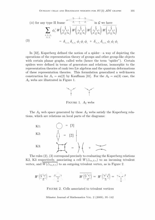
(ii) for any type II frame in G we have
(3)
In [32], Kuperberg defined the notion of a spider—a way of depicting theoperations of the representation theory of groups and other group-like objectswith certain planar graphs, called webs (hence the term “spider”). Certainspiders were defined in terms of generators and relations, isomorphic to therepresentation theories of rank two Lie algebras and the quantum deformationsof these representation theories. This formulation generalized a well-knownconstruction for A1 = su(2) by Kauffman [31]. For the A2 = su(3) case, theA2 webs are illustrated in Figure 1.
Figure 1. A2 webs
The A2 web space generated by these A2 webs satisfy the Kuperberg rela-tions, which are relations on local parts of the diagrams:
K1:
K2:
K3:
The rules (2), (3) correspond precisely to evaluating the Kuperberg relationsK2, K3 respectively, associating a cell W (△α,β,γ) to an incoming trivalent
vertex, and W (△α,β,γ) to an outgoing trivalent vertex, as in Figure 2.
Figure 2. Cells associated to trivalent vertices
Munster Journal of Mathematics Vol. 2 (2009), 95–142
102 David E. Evans and Mathew Pugh
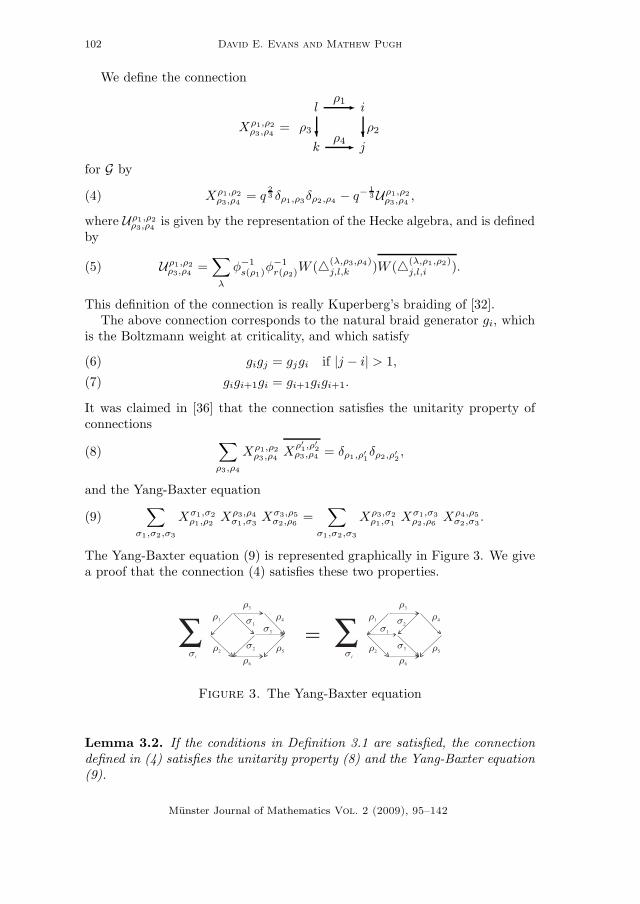
We define the connection
Xρ1,ρ2ρ3,ρ4
=
lρ1- i
k
ρ3 ? ρ4- j
ρ2?
for G by
(4) Xρ1,ρ2ρ3,ρ4
= q23 δρ1,ρ3δρ2,ρ4 − q−
13Uρ1,ρ2
ρ3,ρ4,
where Uρ1,ρ2ρ3,ρ4
is given by the representation of the Hecke algebra, and is definedby
(5) Uρ1,ρ2ρ3,ρ4
=∑
λ
φ−1s(ρ1)φ
−1r(ρ2)
W (△(λ,ρ3,ρ4)j,l,k )W (△(λ,ρ1,ρ2)
j,l,i ).
This definition of the connection is really Kuperberg’s braiding of [32].The above connection corresponds to the natural braid generator gi, which
is the Boltzmann weight at criticality, and which satisfy
gigj = gjgi if |j − i| > 1,(6)
gigi+1gi = gi+1gigi+1.(7)
It was claimed in [36] that the connection satisfies the unitarity property ofconnections
(8)∑
ρ3,ρ4
Xρ1,ρ2ρ3,ρ4
Xρ′
1,ρ′
2ρ3,ρ4 = δρ1,ρ′
1δρ2,ρ′
2,
and the Yang-Baxter equation
(9)∑
σ1,σ2,σ3
Xσ1,σ2ρ1,ρ2
Xρ3,ρ4σ1,σ3
Xσ3,ρ5σ2,ρ6
=∑
σ1,σ2,σ3
Xρ3,σ2ρ1,σ1
Xσ1,σ3ρ2,ρ6
Xρ4,ρ5σ2,σ3
.
The Yang-Baxter equation (9) is represented graphically in Figure 3. We givea proof that the connection (4) satisfies these two properties.
Figure 3. The Yang-Baxter equation
Lemma 3.2. If the conditions in Definition 3.1 are satisfied, the connectiondefined in (4) satisfies the unitarity property (8) and the Yang-Baxter equation(9).
Munster Journal of Mathematics Vol. 2 (2009), 95–142
Ocneanu cells and Boltzmann weights for SU(3) ADE graphs 103
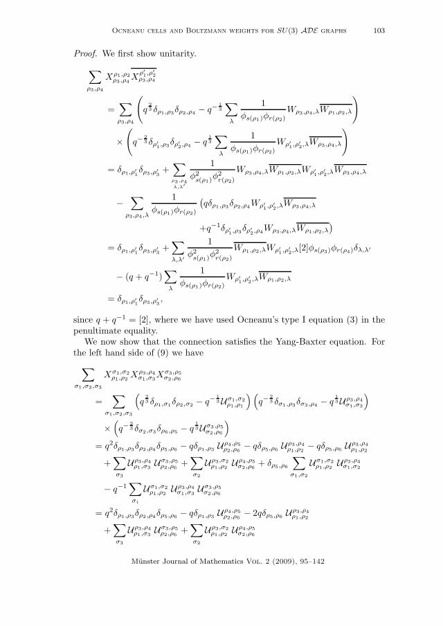
Proof. We first show unitarity.
∑
ρ3,ρ4
Xρ1,ρ2ρ3,ρ4
Xρ′
1,ρ′
2ρ3,ρ4
=∑
ρ3,ρ4
(q
23 δρ1,ρ3δρ2,ρ4 − q−
13
∑
λ
1
φs(ρ1)φr(ρ2)Wρ3,ρ4,λWρ1,ρ2,λ
)
×(
q−23 δρ′
1,ρ3δρ′
2,ρ4− q
13
∑
λ
1
φs(ρ1)φr(ρ2)Wρ′
1,ρ′
2,λWρ3,ρ4,λ
)
= δρ1,ρ′
1δρ3,ρ′
3+∑
ρ3,ρ4λ,λ′
1
φ2s(ρ1)φ
2r(ρ2)
Wρ3,ρ4,λWρ1,ρ2,λWρ′
1,ρ′
2,λWρ3,ρ4,λ
−∑
ρ3,ρ4,λ
1
φs(ρ1)φr(ρ2)
(qδρ1,ρ3δρ2,ρ4Wρ′
1,ρ′
2,λWρ3,ρ4,λ
+q−1δρ′
1,ρ3δρ′
2,ρ4Wρ3,ρ4,λWρ1,ρ2,λ
)
= δρ1,ρ′
1δρ3,ρ′
3+∑
λ,λ′
1
φ2s(ρ1)φ
2r(ρ2)
Wρ1,ρ2,λWρ′
1,ρ′
2,λ[2]φs(ρ3)φr(ρ4)δλ,λ′
− (q + q−1)∑
λ
1
φs(ρ1)φr(ρ2)Wρ′
1,ρ′
2,λWρ1,ρ2,λ
= δρ1,ρ′
1δρ3,ρ′
3,
since q + q−1 = [2], where we have used Ocneanu’s type I equation (3) in thepenultimate equality.
We now show that the connection satisfies the Yang-Baxter equation. Forthe left hand side of (9) we have
∑
σ1,σ2,σ3
Xσ1,σ2ρ1,ρ2
Xρ3,ρ4σ1,σ3
Xσ3,ρ5σ2,ρ6
=∑
σ1,σ2,σ3
(q
23 δρ1,σ1δρ2,σ2 − q−
13Uσ1,σ2
ρ1,ρ1
)(q−
23 δσ1,ρ3δσ3,ρ4 − q
13Uρ3,ρ4
σ1,σ3
)
×(q−
23 δσ2,σ3δρ6,ρ5 − q
13Uσ3,ρ5
σ2,ρ6
)
= q2δρ1,ρ3δρ2,ρ4δρ5,ρ6 − qδρ1,ρ3 Uρ4,ρ5ρ2,ρ6
− qδρ5,ρ6 Uρ3,ρ4ρ1,ρ2
− qδρ5,ρ6 Uρ3,ρ4ρ1,ρ2
+∑
σ3
Uρ3,ρ4ρ1,σ3
Uσ3,ρ5ρ2,ρ6
+∑
σ2
Uρ3,σ2ρ1,ρ2
Uρ4,ρ5σ2,ρ6
+ δρ5,ρ6
∑
σ1,σ2
Uσ1,σ2ρ1,ρ2
Uρ3,ρ4σ1,σ2
− q−1∑
σi
Uσ1,σ2ρ1,ρ2
Uρ3,ρ4σ1,σ3
Uσ3,ρ5σ2,ρ6
= q2δρ1,ρ3δρ2,ρ4δρ5,ρ6 − qδρ1,ρ3 Uρ4,ρ5ρ2,ρ6
− 2qδρ5,ρ6 Uρ3,ρ4ρ1,ρ2
+∑
σ3
Uρ3,ρ4ρ1,σ3
Uσ3,ρ5ρ2,ρ6
+∑
σ2
Uρ3,σ2ρ1,ρ2
Uρ4,ρ5σ2,ρ6
Munster Journal of Mathematics Vol. 2 (2009), 95–142

104 David E. Evans and Mathew Pugh
+ δρ5,ρ6
∑
σ1,σ2λ,λ′
1
φs(ρ1)φr(ρ2)φs(ρ3)φr(ρ4)Wρ1,ρ2,λWσ1,σ2,λWσ1,σ2,λ′Wρ3,ρ4,λ′
− q−1∑
σi,λ
λ′,λ′′
1
φ2s(ρ1)φr(ρ2)φr(ρ4)φs(σ2)φr(ρ6)
Wρ1,ρ2,λWρ3,ρ4,λ′
× Wσ1,σ2,λWσ1,σ3,λ′Wσ2,ρ6,λ′′Wσ1,ρ5,λ′′
= q2δρ1,ρ3δρ2,ρ4δρ5,ρ6 − qδρ1,ρ3 Uρ4,ρ5ρ2,ρ6
− 2qδρ5,ρ6 Uρ3,ρ4ρ1,ρ2
+∑
σ3
Uρ3,ρ4ρ1,σ3
Uσ3,ρ5ρ2,ρ6
+∑
σ2
Uρ3,σ2ρ1,ρ2
Uρ4,ρ5σ2,ρ6
+ δρ5,ρ6
∑
λ,λ′
1
φs(ρ1)φr(ρ2)φs(ρ3)φr(ρ4)Wρ1,ρ2,λWρ3,ρ4,λ′ [2]φr(ρ2)φs(ρ1)δλ,λ′
− q−1∑
λ,λ′
1
φ2s(ρ1)φr(ρ2)φr(ρ4)φr(ρ6)
Wρ1,ρ2,λWρ3,ρ4,λ′
×(δλ,ρ6δλ′,ρ5φr(ρ2)φr(ρ6)φr(ρ4) + δλ,λ′δρ5,ρ6φs(ρ1)φr(ρ2)φr(ρ6)
)
= q2δρ1,ρ3δρ2,ρ4δρ5,ρ6 − qδρ1,ρ3 Uρ4,ρ5ρ2,ρ6
− qδρ5,ρ6 Uρ3,ρ4ρ1,ρ2
+∑
σ3
Uρ3,ρ4ρ1,σ3
Uσ3,ρ5ρ2,ρ6
+∑
σ2
Uρ3,σ2ρ1,ρ2
Uρ4,ρ5σ2,ρ6
− q−1 1
φs(ρ1)Wρ1,ρ2,ρ6Wρ3,ρ4,ρ5 .
Computing the right hand side of (9) in the same way, we arrive at the sameexpression. �
4. Computation of the cells W for ADE graphs
In the remaining sections we will compute cells systems W for each ADEgraph G, with the exception of the graph E(12)
4 .
Let △(α,β,γ)i,j,k be the triangle i
α- j
β- k
γ- i in G. For most of the
ADE graph, using the equations (2) and (3) only, we can compute the cells
up to choice of phase W (△(α,β,γ)i,j,k ) = λα,β,γ
i,j,k |W (△(α,β,γ)i,j,k )| for some λα,β,γ
i,j,k ∈ T,
and also obtain some restrictions on the values which the phases λα,β,γi,j,k may
take. However, for the graph D(n)∗, n = 5, 6, . . . , we impose a Z3 symmetry
on our solutions, whilst for the graphs D(3k), k = 2, 3, . . . , and E(12)1 we seek
an orbifold solution obtained using the identification of the graphs D(3k), E(12)1
as Z3 orbifolds of A(3k), E(12)2 respectively. There is still much freedom in the
actual choice of phases, so that the cell system is not unique. We thereforedefine an equivalence relation between two cell systems:
Definition 4.1. Two families of cells W1, W2 which give a cell system forG are equivalent if, for each pair of adjacent vertices i, j of G, we can find afamily of unitary matrices (u(σ1, σ2))σ1,σ2 , where σ1, σ2 are any pair of edges
Munster Journal of Mathematics Vol. 2 (2009), 95–142

Ocneanu cells and Boltzmann weights for SU(3) ADE graphs 105
from i to j, such that
(10) W1(△(σ,ρ,γ)i,j,k ) =
∑
σ′,ρ′,γ′
u(σ, σ′)u(ρ, ρ′)u(γ, γ′)W2(△(σ′,ρ′,γ′)i,j,k ),
where the sum is over all edges σ′ from i to j, ρ′ from j to k, and γ′ from k toi.
Lemma 4.2. Let W1, W2 be two equivalent families of cells, and X(1), X(2)
the corresponding connections defined using cells W1, W2 respectively. ThenX(1) and X(2) are equivalent in the sense of [18, p.542], i.e. there exists a setof unitary matrices (u(ρ, σ))ρ,σ such that
X(1)ρ1,ρ2ρ3,ρ4
=∑
σi
u(ρ3, σ3)u(ρ4, σ4)u(ρ1, σ1)u(ρ2, σ2)X(2)σ1,σ2σ3,σ4
.
Let Wl(△(σ,ρ,γ)i,j,k ) = λ
(l)σ,ρ,γi,j,k |Wl(△(σ,ρ,γ)
i,j,k )|, for l = 1, 2, be two families of
cells which give cell systems. If |W1(△(σ,ρ,γ)i,j,k )| = |W2(△(σ,ρ,γ)
i,j,k )|, so that W1
and W2 differ only up to phase choice, then the equation (10) becomes
(11) λ(1)σ,ρ,γi,j,k =
∑
σ′,ρ′,γ′
u(σ, σ′)u(ρ, ρ′)u(γ, γ′)λ(2)σ,ρ,γi,j,k .
For graphs with no multiple edges we write △i,j,k for the triangle △(α,β,γ)i,j,k .
For such graphs, two solutions W1 and W2 differ only up to phase choice, and(11) becomes
(12) λ(1)i,j,k = uσuρuγλ
(2)i,j,k,
where uσ, uρ, uγ ∈ T and σ is the edge from i to j, ρ the edge from j to k andγ the edge from k to i.
We will write U (x,y) for the matrix indexed by the vertices of G, with entriesgiven by Uρ1,ρ2
ρ3,ρ4for all edges ρi, i = 1, 2, 3, 4 on G such that s(ρ1) = s(ρ3) = x,
r(ρ2) = r(ρ4) = y, i.e. [U (s(ρ1),r(ρ2))]r(ρ1),r(ρ3) = Uρ1,ρ2ρ3,ρ4
.We first present some relations that the quantum numbers [a]q satisfy, which
are easily checked:
Lemma 4.3.
(i) If q = exp(iπ/n) then [a]q = [n − a]q, for any a = 1, 2, . . . , n − 1,(ii) For any q, [a]q − [a − 2]q = [2a − 2]q/[a − 1]q, for any a ∈ N,(iii) For any q, [a]2q−[a−1]q[a+1]q = 1 and [a]q[a+b]q−[a−1]q[a+b+1]q =
[b + 1]q, for any a ∈ N.
5. A graphs
The infinite graph A(∞) is illustrated in Figure 4, whilst for finite n, thegraphs A(n) are the subgraphs of A(∞), given by all the vertices (λ1, λ2) suchthat λ1 + λ2 ≤ n − 3, and all the edges in A(∞) which connect these ver-tices. The apex vertex (0, 0) is the distinguished vertex. For the triangle△(i1,j1)(i2,j2)(i3,j3) = (i1, j1) - (i2, j2) - (i3, j3) - (i1, j1) in A(n) we
Munster Journal of Mathematics Vol. 2 (2009), 95–142

106 David E. Evans and Mathew Pugh
Figure 4. The infinite graph A(∞)
will use the notation W△(i,j) for the cell W (△(i,j)(i+1,j)(i,j+1)) and W∇(i,j) forthe cell W (△(i+1,j)(i,j+1)(i+1,j+1)).
Theorem 5.1. There is up to equivalence a unique set of cells for A(n), n <∞, given by
W△(k,m) =√
[k + 1][k + 2][m + 1][m + 2][k + m + 1][k + m + 2]/[2],(13)
W∇(k,m) =√
[k + 1][k + 2][m + 1][m + 2][k + m + 2][k + m + 3]/[2],(14)
for all k, m ≥ 0. For the graph A(∞) with Perron-Frobenius eigenvalue α ≥ 3,there is a solution given by replacing [j] by [j]q where q = ex for any x ∈ R
such that α = [3]q.
Proof. Let n < ∞. We first prove the equalities
|W△(k,m)| =√
[k + 1][k + 2][m + 1][m + 2][k + m + 1][k + m + 2]/[2],(15)
|W∇(k,m)| =√
[k + 1][k + 2][m + 1][m + 2][k + m + 2][k + m + 3]/[2],(16)
by induction on k, m. The Perron-Frobenius eigenvector for A(n) is [13]:
(17) φλ =[λ1 + 1]q[λ2 + 1]q[λ1 + λ2 + 2]q
[2].
For the type I frame(0,0)• -
(1,0)• equation (2) gives |W△(0,0)|2 = [2][3],
whilst from the type I frame(1,0)• -
(0,1)• we obtain |W△(0,0)|2+|W∇(0,0)|2 =
[2][3]2, giving |W∇(0,0)|2 = [3][4]. We assume (15) and (16) are true for (k, m) =(p, q). We first show (15) is true for (k, m) = (p + 1, q) and (k, m) = (p, q + 1)
(see Figure 5). From the type I frame(p+1,q+1)• -
(p+1,q)• we get
|W△(p+1,q)|2 + |W∇(p,q)|2 = [p + 2]2[q + 1][q + 2][p + q + 2][p + q + 3]/[2],
Munster Journal of Mathematics Vol. 2 (2009), 95–142

Ocneanu cells and Boltzmann weights for SU(3) ADE graphs 107
and substituting in for |W∇(p,q)|2 we obtain
|W△(p+1,q)|2
= [p + 2][q + 1][q + 2][p + q + 2][p + q + 3]([2][p + 2] − [p + 1])/[2]2
= [p + 2][p + 2][q + 1][q + 2][p + q + 2][p + q + 3]/[2]2.
Similarly, from the type I frame(p,q+1)• -
(p+1,q+1)• we get
|W△(p,q+1)|2 = [p + 1][p + 2][q + 2][q + 3][p + q + 2][p + q + 3]/[2]2,
as required.
Figure 5. Triangles in A(n)
For k, m ≥ 0, the equality in (16) follows from (15) by considering the type
I frame(k+1,m)• -
(k,m+1)• . We get
|W△(k,m)|2 + |W∇(k,m)|2 = [k + 1][k + 2][m + 1][m + 2][k + m + 2]2/[2],
and substituting in for |W△(k,m)|2 we obtain
|W∇(k,m)|2 = [k + 1][k + 2][m + 1][m + 2][k + m + 2]
× ([2][k + m + 2] − [k + m + 1])/[2]2
= [k + 1][k + 2][m + 1][m + 2][k + m + 2][k + m + 3]/[2]2.
Hence (15) and (16) are true for all k, m ≥ 0.There is no restriction on the choice of phase for A(n), so any choice is a so-
lution. We now turn to the uniqueness of these cells. Let W ♯ be another family
of cells, with W ♯△(k,m) = λ(k,m)|W△(k,m)| and W ♯
∇(k,m) = λ′(k,m)|W∇(k,m)| (any
other solution must be of this form since there are no double edges on A(n)).
We label the edges of A(n) by σ(j)i , ρ
(j)i , γ
(j)i , j = 1, . . . , n − 3, i = 1, . . . , j, as
shown in Figure 6.Let us start with the triangle △(0,0)(1,0)(0,1). By (12) we require 1 =
uσ
(1)1
uρ(1)1
uγ(1)1
λ(0,0). Choose uσ
(1)1
= uγ(1)1
= 1 and uρ(1)1
= λ(0,0).
Next consider the triangle △(1,0)(0,1)(1,1). We have 1 = uσ
(2)2
uγ(2)1
λ(0,0)λ′(0,0),
so choose uσ
(2)2
= 1 and uγ(2)1
= λ(0,0)λ′(0,0). Similarly, setting u
σ(2)1
= uγ(2)2
= 1,
Munster Journal of Mathematics Vol. 2 (2009), 95–142

108 David E. Evans and Mathew Pugh
Figure 6. Labels for the vertices and edges of A(n)
uρ(2)1
= λ′(0,0)λ(0,0)λ(1,0) and u
ρ(2)2
= λ(0,1) then (12) is satisfied for the triangles
△(1,0)(2,0)(1,1) and △(0,1)(1,1)(0,2).
Continuing in this way we set uγ(k)k
= 1, uγ(k)i
= uρ(k−1)i
λ′(k−i−1,i−1), for
i = 1, . . . , k − 1, and uσ
(k)i
= 1, uρ(k)i
= uρ(k−1)i
λ′(k−i−1,i−1)λ(k−i,i−1), for i =
1, . . . , k, for each k ≤ n−3. Hence, any choice of λ and λ′ will give an equivalentsolution to (13), (14).
For A(∞), we have Perron-Frobenius eigenvectors φ = (φλ1,λ2) given by
φ(λ1,λ2) =[λ1 + 1]q[λ2 + 1]q[λ1 + λ2 + 2]q
[2]q.
Then the rest of the proof follows as for finite n. �
Using these cells W we obtain the following representation of the Heckealgebra for A(n). We have written the label for the rows (and columns) infront of each matrix.
U ((λ1,λ2),(λ1,λ2+1)) =(λ1+1,λ2)
(λ1−1,λ2+1)
[λ1+2][λ1+1]
√[λ1][λ1+2]
[λ1+1]√[λ1][λ1+2]
[λ1+1][λ1]
[λ1+1]
,(18)
U ((λ1,λ2),(λ1−1,λ2)) =(λ1−1,λ2+1)
(λ1,λ2−1)
[λ2+2][λ2+1]
√[λ2][λ2+2]
[λ2+1]√[λ2][λ2+2]
[λ2+1][λ2]
[λ2+1]
,(19)
U ((λ1,λ2),(λ1+1,λ2−1))(20)
=(λ1+1,λ2)
(λ1,λ2−1)
[λ1+λ2+3][λ1+λ2+2]
√[λ1+λ2+1][λ1+λ2+3]
[λ1+λ2+2]√[λ1+λ2+1][λ1+λ2+3]
[λ1+λ2+2][λ1+λ2+1][λ1+λ2+2]
.
Munster Journal of Mathematics Vol. 2 (2009), 95–142

Ocneanu cells and Boltzmann weights for SU(3) ADE graphs 109
Let e1, e2, e3 be vectors in the direction of the edges from vertex (λ1, λ2) tothe vertices (λ1 +1, λ2), (λ1−1, λ2 +1), (λ1, λ2−1) respectively, and define aninner-product by ej · ek = δj,k − 1/N . Wenzl [42] constructed representationsof the Hecke algebra, which are given in [14] as:
(21)
λ - λ + ek
λ + ej
?
- λ + ej + ek
?= (1 − δjl)
√sjl(λ′ + ej)sjl(λ′ + ek)
sjl(λ′),
where λ = (λ1, λ2) is a vertex on A(n), λ′ = (λ1 + 1, λ2 + 1), and sjl(λ) =sin((π/n)(ej − el) · λ). Note that this weight is 0 when j = l.
Lemma 5.2. The weights in the representation of the Hecke algebra givenabove for A(n) are identical to those in (21).
Proof. For j = l the result is immediate since there is no triangle λ - λ +ej
- λ + 2ej- λ on A(n), and hence the weight in our representation
of the Hecke algebra will be zero also. For an arbitrary vertex λ = (λ1, λ2)of A(n), sjl(λ
′) = sin((π/n)(ej − el) · ((λ1 + 1)e1 − (λ2 + 1)e3)). We willshow the result for j = 1, l = 2 (the other cases follow similarly). We haves12(λ
′) = sin((λ1 + 1)π/n) and s12(λ′ + ej) = s12(λ
′ + e1) = sin((λ1 + 2)π/n).We also have s12(λ
′ + e2) = sin(λ1π/n). Then for k = 1, (21) becomes√
sin2((λ1 + 2)π/n)
sin((λ1 + 1)π/n)=
[λ1 + 2]
[λ1 + 1],
whilst for k = 2, (21) becomes√
sin((λ1 + 2)π/n) sin(λ1π/n)
sin((λ1 + 1)π/n)=
√[λ1][λ1 + 2]
[λ1 + 1],
as required. �
6. D graphs
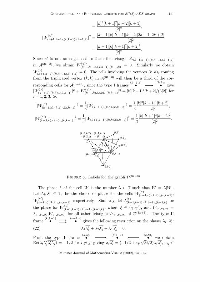
The Perron-Frobenius weights for the vertices of A(n) are invariant underthe Z3 symmetry given by rotation by 2π/3. The graph D(n) is obtained fromthe graph A(n) by taking its Z3 orbifold, as illustrated in Figure 7 for n = 9[17]. The Perron-Frobenius weights for the vertices of D(n) are equal to thecorresponding weights in A(n), except that for n = 3k + 3, for integer k ≥ 1,the vertices (k, k)1, (k, k)2 and (k, k)3 (see Figure 8) which come from the fixedpoint (k, k) of A(3k+3) under the rotation whose Perron-Frobenius weights area third of the weight for the vertex (k, k) of A(3k+3). The absolute values |WA|of the cells for A(n) are also invariant under the rotation.
Let n ≥ 5, n 6≡ 0 mod 3. We will find one solution (up to a choice ofphase) for the cells of D(n) by identifying the absolute values |W (A)| for thecells in A(n) with the absolute values |W (D)| for the corresponding cells in D(n)
when taking the orbifold. Each type I frame in D(n) has a corresponding type Iframe in A(n), and similarly for the type II frames. Since the Perron-Frobenius
Munster Journal of Mathematics Vol. 2 (2009), 95–142

110 David E. Evans and Mathew Pugh
Figure 7. A(9) and its Z3 orbifold D(9)
weights are the same for A(n) and D(n), these |WD| will certainly satisfy (2)and (3) since the |WA| do. As in the case of A(n), there are no restrictions onthe choice of phase. Then we have the following theorem:
Theorem 6.1. Every orbifold solution for the cells of D(n), n 6≡ 0 mod 3, isequivalent to the solution for which the cells in D(n) are equal to the corre-sponding cells in A(n) given in (13), (14).
Proof. The unitaries ui,j ∈ T, for i, j vertices on D(n), may be chosen systemat-ically as in the proof of Theorem 5.1, beginning with u(k,k),(k,k) =
λ(k,k),(k,k),(k,k)1/3
if n = 3k + 4 or u(k+1,k),(k+1,k) = λ(k+1,k),(k+1,k),(k+1,k)1/3
if n = 3k + 5, and proceeding triangle by triangle. �
Now let n = 3k + 3 for some integer k ≥ 1. For q = eiπ/(3k+3), we have[(3k + 3)/2 + i]q = [(3k + 3)/2− i]q where i ∈ Z for k even and i ∈ Z + 1
2 for kodd. In particular we will use [2k + 2 + j] = [k + 1− j] for j ∈ Z. The Perron-Frobenius weights φ(k,k)i
= φ(k,k)/3 = [k + 1]2[2k + 2]/(3[2]) = [k + 1]3/(3[2]),
i = 1, 2, 3. We again find an orbifold solution for the cells for D(3k+3), exceptfor those which involve the vertices (k, k)i, i = 1, 2, 3, which correspond tothe fixed point (k, k) on the graph A(3k+3). Let γ, γ′ be the two edges inthe double edge of D(3k+3), where γ is the edge from (k, k − 1) to (k − 1, k)and γ′ is the edge from (k, k − 1) to (k + 1, k − 1) in A(3k+3) (see Figure 7).
We will use the notation W(ξ)v,(k,k−1),(k−1,k) to denote the cell for the triangle
△v,(k,k−1),(k−1,k) where the edge ξ ∈ {γ, γ′} is used, for v = (k − 1, k − 1),(k + 1, k − 2) or (k, k)i, i = 1, 2, 3. Then in particular we have the following:
|W (γ)(k−1,k−1),(k,k−1),(k−1,k) |2 =
[k]2[k + 1]2[2k][2k + 1]
[2]2
Munster Journal of Mathematics Vol. 2 (2009), 95–142
Ocneanu cells and Boltzmann weights for SU(3) ADE graphs 111
=[k]2[k + 1]2[k + 2][k + 3]
[2]2,
|W (γ′)(k+1,k−2),(k,k−1),(k−1,k) |2 =
[k − 1][k][k + 1][k + 2][2k + 1][2k + 2]
[2]2
=[k − 1][k][k + 1]2[k + 2]2
[2]2.
Since γ′ is not an edge used to form the triangle △(k−1,k−1),(k,k−1),(k−1,k)
in A(3k+3), we obtain W(γ′)(k−1,k−1),(k,k−1),(k−1,k) = 0. Similarly we obtain
W(γ)(k+1,k−2),(k,k−1),(k−1,k) = 0. The cells involving the vertices (k, k)i coming
from the triplicated vertex (k, k) in A(3k+3) will then be a third of the cor-
responding cells for A(3k+3), since the type I frames(k−1,k)• -
(k,k)i• give
|W (γ)(k−1,k),(k,k)i ,(k,k−1)|2 + |W (γ′)
(k−1,k),(k,k)i ,(k,k−1)|2 = [k][k + 1]4[k + 2]/(3[2]) for
i = 1, 2, 3. So
|W (γ)(k−1,k),(k,k)i,(k,k−1)|
2 =1
3|W(k−1,k),(k,k),(k,k−1) |2 =
1
3
[k]2[k + 1]3[k + 2]
[2]2,
|W (γ′)(k−1,k),(k,k)i,(k,k−1)|2 =
1
3|W(k+1,k−1),(k,k),(k,k−1) |2 =
1
3
[k][k + 1]3[k + 2]2
[2]2.
Figure 8. Labels for the graph D(3k+3)
The phase λ of the cell W is the number λ ∈ T such that W = λ|W |.Let λi, λ
′i ∈ T, be the choice of phase for the cells W
(γ)(k−1,k),(k,k)i,(k,k−1),
W(γ′)(k−1,k),(k,k)i ,(k,k−1) respectively. Similarly, let λ
(ξ)(k−1,k−1),(k,k−1),(k−1,k) be
the phase for W(ξ)(k−1,k−1),(k,k−1),(k−1,k) , where ξ ∈ {γ, γ′}, and Wv1,v2,v3 =
λv1,v2,v3 |Wv1,v2,v3 | for all other triangles △v1,v2,v3 of D(3k+3). The type II
frame(k,k−1)• -
-
(k−1,k)• gives the following restriction on the phases λi, λ′i:
(22) λ1λ′1 + λ2λ′
2 + λ3λ′3 = 0.
From the type II frame(k,k)i• -
(k,k−1)• �(k,k)j• we obtain
Re(λiλ′jλ
′iλj) = −1/2 for i 6= j, giving λiλ′
i = (−1/2 + εij
√3i/2)λjλ′
j , εij ∈
Munster Journal of Mathematics Vol. 2 (2009), 95–142

112 David E. Evans and Mathew Pugh
{±1}. Note that εji = −εij , and substituting for λiλ′i with j = i + 1 into (22)
we find ε12 = ε23 = ε31. Then we have
(23) λiλ′i = (−1
2+ ε
√3i
2)λi+1λ′
i+1,
for ε ∈ {±1}, i = 1, 2, 3 (mod 3). Then there are two solutions for the cells ofD(3k+3), W and its complex conjugate W . The solution W is the solution tothe graph where we switch vertices (k, k)2 �- (k, k)3.
Theorem 6.2. Every orbifold solution for the cells of D(3k+3) is given, upto equivalence, by the inequivalent solutions W or its complex conjugate W ,where W is given by
W(γ)(k−1,k),(k,k)i,(k,k−1) = ǫi
[k]√
[k + 1]3[k + 2]√3 [2]
,
W(γ′)(k−1,k),(k,k)i,(k,k−1) = ǫi
[k + 2]√
[k][k + 1]3√3 [2]
,
W(γ)(k−1,k−1),(k,k−1),(k−1,k) =
[k][k + 1]√
[k + 2][k + 3]]
[2],
W(γ′)(k+1,k−2),(k,k−1),(k−1,k) =
[k + 1][k + 2]√
[k − 1][k]
[2],
W(γ′)(k−1,k−1),(k,k−1),(k−1,k) = W
(γ)(k+1,k−2),(k,k−1),(k−1,k) = 0,
where ǫ1 = 1, ǫ2 = e2πi/3 = ǫ3, and all other cells are equal to the correspondingcells in A(3k+3) given in (13), (14).
Proof. Let W ♯ be any orbifold solution for the cells of D(3k+3). Then W ♯ isgiven, for i = 1, 2, 3, by
W♯(γ)(k−1,k),(k,k)i,(k,k−1) = λ♯
i |W(γ)(k−1,k),(k,k)i ,(k,k−1)|,
W♯(γ′)(k−1,k),(k,k)i,(k,k−1) = λ♯
i′|W (γ′)
(k−1,k),(k,k)i ,(k,k−1)|,
W♯(ξ)(k−1,k−1),(k,k−1),(k−1,k) =
λ♯(ξ)(k−1,k−1),(k,k−1),(k−1,k) |W
♯(ξ)(k−1,k−1),(k,k−1),(k−1,k) |,
where ξ ∈ {γ, γ′}, and W ♯v1,v2,v3
= λ♯v1,v2,v3
|Wv1,v2,v3 | for all other triangles
△v1,v2,v3 of D(3k+3), and where the choice of λ♯i , λ♯
i′ satisfy condition (23)
with ε = 1. We need to find a family of unitaries {uρ} for edges ρ 6= γ′ of
D(3k+3), where uγ = (uγ(ξ, ξ′)), ξ, ξ′ ∈ {γ, γ′}, is a 2 × 2 unitary matrix, anduρ ∈ T for all other ρ. These unitaries must satisfy (11) and (12), i.e. ǫl =
uµluµ′
l(uγ(γ, γ)λ♯
l + uγ(γ, γ′)λ♯l′) and ǫl = uµl
uµ′
l(uγ(γ′, γ)λ♯
l + uγ(γ′, γ′)λ♯l′),
for l = 1, 2, 3, and
1 = uσ1uσ2
∑
ξ′
u(ξ, ξ′)λ♯(ξ′)(k−1,k−1),(k,k−1),(k−1,k) ,
Munster Journal of Mathematics Vol. 2 (2009), 95–142

Ocneanu cells and Boltzmann weights for SU(3) ADE graphs 113
1 = uσ′
1uσ′
2
∑
ξ′
u(ξ, ξ′)λ♯(ξ′)(k+1,k−2),(k,k−1),(k−1,k) .
For all other triangles △(ρ1,ρ2,ρ3)p1,p2,p3 of D(3k+3) we require 1 = uρ1uρ2uρ3λ
♯p1,p2,p3
.For uγ we choose uγ(γ, γ) = 1, uγ(γ, γ′) = uγ(γ′, γ) = 0 and uγ(γ′γ′) =
λ♯1λ
♯1. We set uµ′
l= 1 and uµl
= ǫlλ♯l , for l = 1, 2, 3, and uσ1 = uσ′
1= 1,
uσ2 = λ♯(γ)(k−1,k−1),(k,k−1),(k−1,k) and uσ′
2= λ
♯(γ′)(k+1,k−2),(k,k−1),(k−1,k) .
Figure 9. Triangles △(ρ(1),ρ(2),ρ(3))(i,j),(i−1,j+1),(i,j+1) and △(ρ(1)′,ρ(2)′,ρ(3)′)
(i−1,j),(i,j),(i−1,j+1)
For the remaining triangles we proceed as follows. Let m = 2k − 2. For
each triangle △(ρ(1),ρ(2),ρ(3))(i,j),(i−1,j+1),(i,j+1) as in Figure 9 (and similarly for triangles
△(i,j),(i−1,j+1),(i,j+1)) such that i+j = m, if either uρ(1) or uρ(2) hasn’t yet been
assigned a value we set it to be 1, and set uρ(3) = uρ(1)uρ(2)λ♯(i,j),(i−1,j+1),(i,j+1) .
Next, for each triangle △(ρ(1)′,ρ(2)′,ρ(3)′)(i−1,j),(i,j),(i−1,j+1) as in Figure 9 (and similarly
for triangles △(i+1,j−1),(i,j),(i+1,j)) such that i + j = m, if either uρ(1)′ oruρ(2)′ hasn’t yet been assigned a value we set it to be 1, and set uρ(3)′ =
uρ(1)′uρ(2)′λ♯(i−1,j),(i,j),(i−1,j+1) . We then set m = 2k − 3 and repeat the above
steps. Continuing in this way, for m = 2k − 4, . . . , 3, we find the required uni-taries {uρ}. The proof for the uniqueness of the complex conjugate solutioncan be shown similarly.
For the solutions W and W to be equivalent, we require unitaries as abovesuch that
ǫl = uµluµ′
l(uγ(γ, γ)ǫl +
√[k + 2]√
[k]uγ(γ, γ′)ǫl),
ǫl = uµluµ′
l(
√[k]√
[k + 2]uγ(γ′, γ)ǫl + uγ(γ′, γ′)ǫl),
for l = 1, 2, 3. This forces uγ(γ, γ) = uγ(γ′, γ′) = 0, uγ(γ, γ′) =√
[k]/√
[k + 2]
and uγ(γ′, γ) =√
[k + 2]/√
[k]. But then uγ is not a unitary. �
Using the cells W we obtain the following representation of the Hecke alge-bra for D(3k+3), we use the notation v(γ) if the path uses the edge γ, where v
Munster Journal of Mathematics Vol. 2 (2009), 95–142

114 David E. Evans and Mathew Pugh
is a vertex of D(3k+3):
U ((k−1,k−1),(k−1,k)) =
(k,k−1)(γ)
(k,k−1)(γ′)
(k−2,k)
[k+1][k] 0
√[k−1][k+1]
[k]
0 0 0√[k−1][k+1]
[k] 0 [k−1][k]
= U ((k,k−1),(k−1,k−1)) with rows labelled by (k − 1, k)(γ), (k − 1, k)(γ′),
U ((k+1,k−2),(k−1,k)) =
(k,k−1)(γ)
(k,k−1)(γ′)
(k−2,k)
0 0 0
0 [k+1][k+2]
√[k+1][k+3]
[k+2]
0
√[k+1][k+3]
[k+2][k+3][k+2]
= U ((k,k−1),(k+1,k−2)) with rows labelled by (k − 1, k)(γ), (k − 1, k)(γ′),
(k, k − 2),
U ((k,k−1),(k,k)i) =(k−1,k)(γ)
(k−1,k)(γ′)
[k][k+1] ǫi
√[k][k+2]
[k+1]
ǫi
√[k][k+2]
[k+1][k+2][k+1]
,
= U ((k,k)i,(k−1,k)) with rows labelled by (k, k − 1)(γ), (k, k − 1)(γ′),
U ((k−1,k),(k,k−1)) =
(k,k)1
(k,k)2
(k,k)3
(k−1,k−1)
(k+1,k−2)
[2][k + 1]a ǫa ǫa b c
ǫa [2][k + 1]a ǫa ǫ2b ǫ2c
ǫa ǫa [2][k + 1]a ǫ2b ǫ2c
b ǫ2b ǫ2b[k+3][k+2] 0
c ǫ2c ǫ2c 0 [k−1][k]
,
where ǫ = ǫ2[k] + ǫ2[k + 2] and
a =[k + 1]
3[k][k + 2], b =
√[k + 1][k + 3]√
3 [k + 2], c =
√[k − 1][k + 1]√
3 [k].
Another representation of the Hecke algebra is given by taking the complexconjugates of the weights in the representation above.
In [25], Fendley gives Boltzmann weights for D(6), which at criticality andwith the parameter u = 1, give a representation of the Hecke algebra. Howeverthese Boltzmann weights are not equivalent to the representation of the Heckealgebra using the cells W or W . To see this, we use a similar labelling for thegraph D(6) as in [25]- see Figure 10.
Consider the weight [U(3r,2)
]γ,γ′ , where we label the rows and columns byγ, γ′ to denote which edge from 1 to 2 is used for the path of length 2 from3r to 2, r = 0, 1, 2, and the weight U is the complex conjugate of that givenabove, i.e. it is the weight given by the solution W for the cells of D(6). Then
Munster Journal of Mathematics Vol. 2 (2009), 95–142

Ocneanu cells and Boltzmann weights for SU(3) ADE graphs 115
Figure 10. Labelling the graph D(6)
for equivalence we require a unitary u3r,1 ∈ T and a 2 × 2 unitary matrix uγ
such that
ǫr2
√[3]
[2]= |u3r,1|2
(uγ(γ, γ)uγ(γ′, γ)
1
[2]+ uγ(γ, γ)uγ(γ′, γ′)ǫr
2
√[3]
[2]
+uγ(γ, γ′)uγ(γ′, γ)ǫr2
√[3]
[2]+ uγ(γ, γ′)uγ(γ′, γ′)
[3]
[2]
).(24)
Since uγ is independent of r, for (24) to be satisfied for each r = 0, 1, 2, we
require uγ(γ, γ)uγ(γ′, γ′) = 1 and the other terms to be zero, which givesuγ(γ, γ′) = uγ(γ′, γ) = 0 and uγ(γ′, γ′) = (uγ(γ, γ))−1. But now if we consider
the weight [U(1,3r)
]γ,γ′ , with u2,3r∈ T, we have
ǫr2
√[3]
[2]= |u2,3r
|2(
uγ(γ, γ)uγ(γ′, γ)1
[2]+ uγ(γ, γ)uγ(γ′, γ′)ǫr
2
√[3]
[2]
+uγ(γ, γ′)uγ(γ′, γ)ǫr2
√[3]
[2]+ uγ(γ, γ′)uγ(γ′, γ′)
[3]
[2]
),
but [U(1,3r)
]γ,γ′ = ǫr2
√[3]
[2] , for r = 0, 1, 2. We obtain a similar contradiction
when considering the weights U defined using the solution W for the cells.
Suppose however that the Boltzmann weight denoted by W(e1,f3r)e2,e2 in [25] is
the complex conjugate of that given. Then the Boltzmann weights at criticalityof Fendley [25] are equivalent to the representation of the Hecke algebra givenby the solution W for the cells of D(6). We choose a family of unitaries u0,1 =u2,0 = u2,3r
= 1, u3r,1 = ǫr2, r = 0, 1, 2, and choose uγ to be the 2 × 2 identity
matrix.
7. A∗ graphs
The infinite series of graphs A(n)∗ are illustrated in Figure 11. The graphsA(2n+1)∗ and A(2n)∗ are slightly different.
First we consider the graphs A(2n+1)∗. The Perron-Frobenius weights onthe vertices are given by φi = [2i − 1], i = 1, . . . , n.
Munster Journal of Mathematics Vol. 2 (2009), 95–142

116 David E. Evans and Mathew Pugh
Figure 11. A(n)∗ for n = 4, 5, 6, 7, 8, 9
Theorem 7.1. There is up to equivalence a unique set of cells for A(2n+1)∗,n < ∞, given by
Wi−1,i,i =
√[i][2i − 3][2i − 1]√
[i − 1], i = 2, . . . , n,
Wi,i,i+1 =
√[i − 1][2i − 1][2i + 1]√
[i], i = 2, . . . , n − 1,
Wi,i,i = (−1)i+1 [2i − 1]√[i − 1][i]
, i = 2, . . . , n.
Proof. Using (2), (3) we obtain
|Wi−1,i,i|2 =[i][2i − 3][2i − 1]
[i − 1], i = 2, . . . , n,(25)
|Wi,i,i+1|2 =[i − 1][2i − 1][2i + 1]
[i], i = 2, . . . , n − 1,(26)
|Wi,i,i|2 =[2i − 1]2
[i − 1][i], i = 2, . . . , n.(27)
Let Wi,j,k = λi,j,k|Wi,j,k| for λi,j,k ∈ T. From type II frames we have therestriction
(28) λ3i,i,i+1λi+1,i+1,i+1 = −λ3
i,i+1,i+1λi,i,i,
for i = 2, . . . , n − 1. Let W ♯i,j,k = λ♯
i,j,k|Wi,j,k| be any other solution to
the cells, where the λ♯ satisfy (28). We need to find a family of unitaries{ui,j}, where ui,j is the unitary for the edge from vertex i to vertex j on
A(2n+1)∗, which satisfy (12), i.e. −1 = u32l,2lλ
♯2l,2l,2l for l = 1, . . . , ⌊n/2⌋,
and 1 = uiujukλ♯i,j,k for all other triangles △i,j,k. We choose u1,2 = 1,
u2,1 = −(λ♯2,2,2)
1/3λ♯1,2,2, u2,2 = −(λ♯
2,2,2)1/3, and for i = 2, . . . , n−1, ui,i+1 = 1
ui+1,i = −(λ♯2,2,2)
1/3λ♯2,3,3λ
♯3,4,4 · · ·λ♯
i−1,i,iλ♯2,2,3λ
♯3,3,4 · · ·λ♯
i,i,i+1, and ui+1,i+1 =
−(λ♯2,2,2)
1/3λ♯2,2,3λ
♯3,3,4 · · ·λ♯
i,i,i+1λ♯2,3,3λ
♯3,4,4 · · ·λ♯
i,i+1,i+1. �
For A(2n+1)∗, the above cells W give the following representation of theHecke algebra:
U (i,i+1) =i
i+1
[i−1][i]
√[i−1][i+1]
[i]√[i−1][i+1]
[i][i+1][i]
,
Munster Journal of Mathematics Vol. 2 (2009), 95–142

Ocneanu cells and Boltzmann weights for SU(3) ADE graphs 117
U (i,i−1) =i−1
i
[i−2][i−1]
√[i−2][i]
[i−1]√[i−2][i]
[i−1][i]
[i−1]
,
U (i,i) =
i−1
i
i+1
[i][2i−3][i−1][2i−1]
(−1)i+1√
[2i−3]
[i−1]√
[2i−1]
√[2i−3][2i+1]
[2i−1]
(−1)i+1√
[2i−3]
[i−1]√
[2i−1]
1[i−1][i]
(−1)i+1√
[2i+1]
[i]√
[2i−1]√[2i−3][2i+1]
[2i−1]
(−1)i+1√
[2i+1]
[i]√
[2i−1]
[i−1][2i+1][i][2i−1]
.
In [4], Behrend and Evans give Boltzmann weights
W
(a d
b c
∣∣∣∣∣u)
,
which at criticality, with u = 1, give a representation of the Hecke algebra.(Note, these Boltzmann weights are not to be confused with the Ocneanu cellsW .)
Lemma 7.2. The weights in the representation of the Hecke algebra givenabove for A(2n+1)∗ are equivalent to the Boltzmann weights at criticality givenby Behrend-Evans in [4].
Proof. To make our notation the same as that of [4] one replaces i with (a +1)/2. Then it is easily checked that the absolute values of our weights givenabove are equal to those for the Boltzmann weights in [4], setting q = 0, in allbut a few cases. We will show that the absolute values in these other cases arealso equal. For [U (i,i)]i+1,i+1, the Boltzmann weight in [4] is
[a + 2] − [a + 2]/[a]
[a + 1]=
[a + 2]
[a][a + 1]([a] − [1]) =
[a + 2]
[a][a + 1]
[ 12 (a − 1)][a + 1]
[ 12 (a + 1)],
which is equal to our weight, and similarly for [U (i,i)]i−1,i−1. For [U (i,i)]i,i wehave to do the most work. From [4] its value is
(29)1
[3]
([2] − [a + 2][12 (a − 5)]
[a][12 (a + 1)]− [a − 2][12 (a + 5)]
[a][12 (a − 1)]
).
Writing this expression over a common denominator, and using (1), we canwrite the numerator as
[2][a]([2] + [4] + · · · + [a − 1]) − [a + 2]([3] + [5] + · · · + [a − 4])
− [a − 2]([3] + [5] + · · · + [a + 2])
= [a]([1] + [3] + [3] + [5] + · · · + [a − 2] + [a])
− ([a + 2] + [a − 2])([3] + [5] + · · · + [a − 4])
− [a − 2]([a − 2] + [a] + [a + 2])
= [a] + (2[a] − [a + 2] − [a − 2])([3] + [5] + · · · + [a − 4] + [a − 2])
+ [a]2 − [a − 2][a]
Munster Journal of Mathematics Vol. 2 (2009), 95–142

118 David E. Evans and Mathew Pugh
= [a] + ([a] − [a + 2])([3] + [5] + · · · + [a − 2])
+ ([a] − [a − 2])([3] + [5] + · · · + [a − 2] + [a])
= [a] + [(a − 3)/2][(a + 1)/2]([a] − [a + 2])
+ [(a − 1)/2][(a + 3)/2]([a] − [a − 2]).
Now
[(a − 3)/2][(a + 1)/2]([a] − [a + 2])
= [(a − 3)/2]([(a + 1)/2] + [(a + 5)/2] + · · · + [(3a − 1)/2]
− [(a + 5)/2] − [(a + 9)/2]− · · · − [(3a + 3)/2])
= [(a − 3)/2]([(a + 1)/2] − [(3a + 3)/2])
= [3] + [5] + · · · + [a − 2] − [a + 4] − [a + 6] − · · · − [2a − 1],
and
[(a − 1)/2][(a + 3)/2]([a] − [a − 2])
= [(a − 1)/2]([(a + 1)/2] + [(a + 3)/2] + · · · + [(3a + 1)/2]
− [(a − 5)/2] − [(a − 1)/2]− · · · − [(3a − 3)/2])
= [(a − 1)/2]([(3a + 1)/2]− [(a − 5)/2])
= [a + 2] + [a + 4] + · · · + [2a − 1] − [3] − [5] − · · · − [a − 4].
Then we find that the numerator is given by [a] + [a− 2]+ [a +2] = [3][a], and(29) becomes
[3][a]
[3][a][12 (a − 1)][12 (a + 1)]=
1
[ 12 (a − 1)][12 (a + 1)]
as required. To show equivalence, we need unitaries ui,j ∈ T, for vertices i, j
of A(n)∗ such that
1 = ui,iui+1,i+1, 1 = ui,iui−1,i−1, −1 = ui,i−1ui−1,iui,i+1ui+1,i,
(−1)i = u2i,iui,i+1ui+1,i, (−1)i+1 = u2
i,iui,i−1ui−1,i.
Then we set ui,i = 1 for all i, and for m = 0, . . . , (n − 2)/2, u2m+1,2m =u2m,2m+1 = u2m+2,2m+1 = 1 and u2m+1,2m+2 = −1. �
For the graphsA(4n)∗ (illustrated in Figure 11) the Perron-Frobenius weightson the vertices are given by φi = [2i]/[2], i = 1, . . . , 2n − 1. There are nowtwo solutions W+, W− for the cells for A(4n)∗, which are not equivalent since|W+| 6= |W−| and the graph A(4n)∗ does not contain any multiple edges.
Theorem 7.3. The cells for A(4n)∗, n < ∞, are given, up to equivalence, bythe inequivalent solutions W+, W−:
W±i,i,i+1 =
√[2i][2i + 2]
[2]√
[2i + 1]
√[2i]∓ [1], i = 1, . . . , 2n− 2,
Munster Journal of Mathematics Vol. 2 (2009), 95–142

Ocneanu cells and Boltzmann weights for SU(3) ADE graphs 119
W±i,i+1,i+1 =
√[2i][2i + 2]
[2]√
[2i + 1]
√[2i + 2] ± [1], i = 1, . . . , 2n − 2,
W±i,i,i =
(−1)i+1
√[2i]
[2]√
[2i − 1][2i + 1]
√[2][2i] ± [4i], i = 1, . . . , n − 1,
(−1)n+1 [2n]√[2][2n− 1][2n + 1]
, i = n,
(−1)i+1
√[2i]
[2]√
[2i − 1][2i + 1]
√[2][2i] ∓ [8n− 4i],
i = n + 1, . . . , 2n − 1.
Proof. The proof follows in a similar way to the A(2n+1)∗ case. �
For the graphs A(4n+2)∗ (illustrated in Figure 11) the Perron-Frobeniusweights on the vertices are again given by φi = [2i]/[2], i = 1, . . . , 2n. Thereare again two inequivalent solutions W+, W− for the cells of A(4n+2)∗.
Theorem 7.4. The cells for A(4n+2)∗, n < ∞, are given, up to equivalence,by the inequivalent solutions W+, W−:
W±i,i,i+1 =
√[2i][2i + 2]
[2]√
[2i + 1]
√[2i] ∓ [1], i = 1, . . . , 2n− 1,
W±i,i+1,i+1 =
√[2i][2i + 2]
[2]√
[2i + 1]
√[2i + 2] ± [1], i = 1, . . . , 2n − 1,
W±i,i,i =
(−1)i+1
√[2i]
[2]√
[2i − 1][2i + 1]
√[2][2i]± [4i], i = 1, . . . , n,
(−1)i+1
√[2i]
[2]√
[2i − 1][2i + 1]
√[2][2i]∓ [8n + 4 − 4i],
i = n + 1, . . . , 2n.
Proof. The proof again follows in a similar way to the A(2n+1)∗ case. �
For A(2n)∗, the cells W+ above give the following representation of the Heckealgebra:
U (i,i+1) =i
i+1
[2i]−[1][2i+1]
√([2i]−[1])([2i+2]+[1])
[2i+1]√([2i]−[1])([2i+2]+[1])
[2i+1][2i+2]+[1]
[2i+1]
,
U (i,i−1) =i−1
i
[2i−2]−[1][2i−1]
√([2i−2]−[1])([2i]+[1])
[2i−1]√([2i−2]−[1])([2i]+[1])
[2i−1][2i]+[1][2i−1]
,
Munster Journal of Mathematics Vol. 2 (2009), 95–142

120 David E. Evans and Mathew Pugh
U (i,i) =
i−1
i
i+1
[2i−2]([2i]+[1])[2i][2i+1] (−1)i+1√xa+
√[2i−2][2i−1][2i+2]
[2i]√
[2i+1]
(−1)i+1√xa+ x (−1)i+1√xa−√[2i−2][2i−1][2i+2]
[2i]√
[2i+1](−1)i+1√xa−
[2i+2]([2i]−[1])[2i][2i+1]
,
where, a± = [2i ∓ 2]([2i]± [1])/[2i][2i + 1], and for m > 0, if n = 2m,
x =
[2][2i]+[4i][2i−1][2i][2i+1] for i = 1, . . . , m − 1,
[2][2m−1]2 for i = m,
[2][2i]−[4n−4i][2i−1][2i][2i+1] for i = m + 1, . . . , 2m − 1,
,
and if n = 2m + 1,
x =
[2][2i]+[4i][2i−1][2i][2i+1] for i = 1, . . . , m,
[2][2i]−[4n−4i][2i−1][2i][2i+1] for i = m + 1, . . . , 2m,
.
Lemma 7.5. The weights in the representation of the Hecke algebra givenabove for A(2n)∗ are equivalent to the Boltzmann weights at criticality given byBehrend-Evans in [4].
Proof. To make our notation the same as that of [4] one replaces i with a/2. Tosee that the absolute values of our weights are equal to those of the Boltzmannweights in [4] one needs the following relations on the quantum numbers:
[2i] + [1] =[2i + 1]q′ [4i + 2]q′
[2i − 1]q′
, [2i] − [1] =[2i − 1]q′ [4i + 2]q′
[2i + 1]q′
,
where q′ =√
q (q = eiπ/n). Again, a bit more work is required for [U (i,i)]i,i.
For equivalence we make the same choice of (ui,j)i,j as for A(2n+1)∗. �
8. D∗ graphs
The graphs D(n)∗ are illustrated in Figure 12. We label its vertices by il, jl
and kl, l = 1, . . . , ⌊(n−1)/2⌋, which we have illustrated in Figure 12 for n = 9.We consider first the graphs D(2n+1)∗. The Perron-Frobenius weights are
φil= φjl
= φkl= [2l − 1], l = 1, . . . , n. Since the graph has a Z3 symmetry,
we will seek Z3-symmetric solutions (up to choice of phase), i.e. |Wip,jq,kr|2 =
|Wiq ,jr ,kp|2 = |Wir ,jp,kq
|2 =: |Wp,q,r|2, p, q, r ∈ {1, . . . , n}. Using this notation,we have the following equations from type I frames:
|W1,2,2|2 = [2][3],(30)
|Wl,l,l+1|2 + |Wl,l+1,l+1|2 = [2][2l − 1][2l + 1], l = 2, . . . , n − 1,(31)
|Wl−1,l,l|2 + |Wl,l,l|2 + |Wl,l,l+1|2 = [2][2l − 1]2, l = 2, . . . , n − 1,(32)
|Wn−1,n,n|2 + |Wn,n,n|2 = [2]3,(33)
Munster Journal of Mathematics Vol. 2 (2009), 95–142

Ocneanu cells and Boltzmann weights for SU(3) ADE graphs 121
Figure 12. D(n)∗ for n = 6, 7, 8, 9
and from type II frames we have:
(34) |Wl−1,l,l|2|Wl,l,l+1|2 = [2l − 3][2l − 1]2[2l + 1],
for l = 2, . . . , n − 1, and
(35) |Wl−1,l,l|2(1
[2l − 3]|Wl−1,l−1,l|2 +
1
[2l − 1]|Wl,l,l|2) = [2l − 3][2l − 1]2,
for l = 2, . . . , n, which are exactly those for the type I and type II frames forthe graph A(2n+1)∗. Since the Perron-Frobenius weights and Coxeter numberare also the same as for A(2n+1)∗, the cells |Wp,q,r,| follow.
From the type II frame consisting of the vertices il, jl, il+1 and jl+1 we havethe following restriction on the choice of phase
λil,jl,kl+1λil,jl+1,kl
λil+1,jl,klλil+1,jl+1,kl+1
(36)
= −λil,jl,klλil,jl+1,kl+1
λil+1,jl,kl+1λil+1,jl+1,kl
.
Theorem 8.1. Every Z3-symmetric solution for the cells W of D(2n+1)∗, n <∞, is equivalent to the solution
Wi1,j2,k2 = Wi2,j1,k2 = Wi2,j2,k1 =√
[2][3],
Wil,jl+1,kl+1= Wil+1,jl,kl+1
= Wil+1,jl+1,kl=
√[l + 1][2l − 1][2l + 1]√
[l],
Wil,jl,kl+1= Wil,jl+1,kl
= Wil+1,jl,kl=
√[l − 1][2l − 1][2l + 1]√
[l],
Wil,jl,kl= (−1)l+1 [2l − 1]√
[l − 1][l], Win,jn,kn
= (−1)n+1 [2n− 1]√[n − 1][n]
,
for l = 2, . . . , n − 1.
Proof. Let W ♯ be any Z3-symmetric solution for the cells of D(2n+1)∗, wherethe choice of phase satisfies the condition (36). Since D(2n+1)∗ does not contain
any multiple edges, we must have |W ♯ijk | = |Wijk | for every triangle △ijk of
Munster Journal of Mathematics Vol. 2 (2009), 95–142

122 David E. Evans and Mathew Pugh
D(2n+1)∗. We need to find a family of unitaries {up,q}, where up,q is the uni-
tary for the edge from vertex p to vertex q on D(2n+1)∗, which satisfy (12), i.e.
−1 = ui2l,j2luj2l,k2l
uk2l,i2lλ♯
i2l,j2l,k2lfor the triangle △i2l,j2l,k2l
, l = 1, . . . , ⌊n/2⌋,and 1 = up1up2up3λp1,p2,p3 for all other triangles on D(2n+1)∗. For triangles
involving the outermost vertices, we require that 1 = ui1,j2uj2,k2uk2,i1λ♯i1,j2,k1
,
1 = ui2,j1uj1,k2uk2,i2λ♯i2,j1,k2
, 1 = ui2,j2uj2,k1uk1,i2λ♯i2,j2,k1
and also −1 =
ui2,j2uj2,k2uk2,i2λ♯i2,j2,k2
. So we choose ui1,j2 = uj1,k2 = uk1,i2 = uj2,k2 =
uk2,i2 = 1, ui2,j1 = λ♯i2,j1,k2
, uk2,i1 = λ♯i1,j2,k2
, ui2,j2 = −λ♯i2,j2,k2
and uj2,k1 =
−λ♯i2,j2,k2
λ♯i2,j2,k1
. Next consider the equations 1 = ui2,j3uj3,k2uk2,i2λ♯i2,j3,k2
,
1 = ui3,j2uj2,k2uk2,i3λ♯i3,j2,k2
and 1 = ui2,j2uj2,k3uk3,i2λ♯i2,j2,k3
. We make the
following choices: ui2,j3 = uj2,k3 = uk2,i3 = 1, ui3,j2 = λ♯i3,j2,k2
, uj3,k2 =
λ♯i2,j3,k2
and uk3,i2 = −λ♯i2,j2,k2
λ♯i2,j2,k3
. Next we consider the equations
1 = ui2,j3uj3,k3uk3,i2λ♯i2,j3,k3
= −uj3,k3λ♯i2,j2,k2
λ♯i2,j2,k3
λ♯i2,j3,k3
,
1 = ui3,j2uj2,k3uk3,i3λ♯i3,j2,k3
= uk3,i3λ♯i3,j2,k2
λ♯i3,j2,k3
,
1 = ui3,j3uj3,k2uk2,i3λ♯i3,j3,k2
= ui3,j3λ♯i2,j3,k2
λ♯i3,j3,k2
.
We make the choices ui3,j3 = λ♯i2,j3,k2
λ♯i3,j3,k2
, uk3,i3 = λ♯i3,j2,k2
λ♯i3,j2,k3
and
uj3,k3 = −λ♯i2,j2,k3
λ♯i2,j2,k2
λ♯i2,j3,k3
. Then ui3,j3uj3,k3uk3,i3λ♯i3,j3,k3
=
−λ♯i2,j3,k2
λ♯i3,j3,k2
λ♯i2,j2,k3
λ♯i2,j2,k2
λ♯i2,j3,k3
λ♯i3,j2,k2
λ♯i3,j2,k3
= −1, by (36), as re-quired. Continuing in this way we are done. �
For D(2n+1)∗, the Hecke representation for the cells W above is given bythe Hecke representation for A(2n+1)∗, where [U (il,kr)]jm,jp
= [U (jl,ir)]km,kp=
[U (kl,jr)]im,ipare given by the weights [U (l,r)]m,p for A(2n+1)∗, for any l, m, p, r
allowed by the graph.We now consider the graphs D(2n)∗. The Perron-Frobenius weights are
φil= φjl
= φkl= [2l]/[2], and we again assume |Wip,jq,kr
|2 = |Wiq ,jr,kp|2 =
|Wir ,jp,kq|2 =: |Wp,q,r|2, where p, q, r ∈ {1, . . . , n − 1}. Then as for D(2n+1)∗,
the Z3-symmetric solution for the cells follows from the solution for A(2n)∗,and we have the same restriction (36) on the choice of phase. So we have
Theorem 8.2. For n < ∞, the Z3-symmetric solution for the cells of D(4n)∗
are given by
W±il,jl,kl+1
= W±il,jl+1,kl
= W±il+1,jl,kl
=
√[2l][2l + 2]
[2]√
[2l + 1]
√[2l] ∓ [1],
l = 2, . . . , 2n − 2,
Munster Journal of Mathematics Vol. 2 (2009), 95–142

Ocneanu cells and Boltzmann weights for SU(3) ADE graphs 123
W±il,jl+1,kl+1
= W±il+1,jl,kl+1
= W±il+1,jl+1,kl
=
√[2l][2l + 2]
[2]√
[2l + 1]
√[2l + 2] ± [1],
l = 1, . . . , 2n − 2,
W±il,jl,kl
=
(−1)l+1
√[2l]
[2]√
[2l − 1][2l + 1]
√[2][2l]± [4l], l = 1, . . . , n − 1,
(−1)n+1 [2n]√[2][2n− 1][2n + 1]
, l = n,
(−1)l+1
√[2l]
[2]√
[2l − 1][2l + 1]
√[2][2l]∓ [8n − 4l],
l = n + 1, . . . , 2n − 1,
and the Z3-symmetric solution for the cells of D(4n+2)∗ are
W±il,jl,kl+1
= W±il,jl+1,kl
= W±il+1,jl,kl
=
√[2l][2l + 2]
[2]√
[2l + 1]
√[2l]∓ [1],
l = 2, . . . , 2n − 1,
W±il,jl+1,kl+1
= W±il+1,jl,kl+1
= W±il+1,jl+1,kl
=
√[2l][2l + 2]
[2]√
[2l + 1]
√[2l + 2] ± [1],
l = 1, . . . , 2n − 1,
W±il,jl,kl
=
(−1)l+1
√[2l]
[2]√
[2l − 1][2l + 1]
√[2][2l]± [4l], l = 1, . . . , n,
(−1)l+1
√[2l]
[2]√
[2l − 1][2l + 1]
√[2][2l]∓ [8n + 4 − 4l],
l = n + 1, . . . , 2n.
The uniqueness of these solutions follows in the same way as for D(2n+1)∗.If W+ is a solution for the cells of D(2n)∗, then W− is a solution for the cells ofthe graph where we switch vertices il �- in−l, jl
�- jn−l and kl�- kn−l,
for all l = 1, . . . , n − 1.For D(2n)∗, the Hecke representation for the cells W+ above is given by
the Hecke representation for A(2n)∗, where [U (il,kr)]jm,jp= [U (jl,ir)]km,kp
=
[U (kl,jr)]im,ipare given by the weights [U (l,r)]m,p for A(2n)∗, for any l, m, p, r
allowed by the graph.In [14], di Francesco and Zuber gave a representation of the Hecke algebra
for the graph D(6)∗, with the absolute values of the weights there equal to thosefor our weights given above. The two Hecke representations are not identicalas the weights in [14] involve the complex variable i. However it has not beenpossible to determine whether or not the two representations are equivalent asthere are known to be a number of typographical errors in the representationin [14].
Munster Journal of Mathematics Vol. 2 (2009), 95–142

124 David E. Evans and Mathew Pugh
9. E(8)
We will label the vertices of the exceptional graph E(8) in the following way.We will label the six outmost vertices by il and the six inmost vertices byjl, l = 1, . . . , 6, such that there are edges from il to jl and from jl to il+1.The Perron-Frobenius weights on the vertices are φil
= 1, φjl= [3]. With
[a] = [a]q, q = eiπ/8, we have [4]/[2] =√
2.
Figure 13. E(8) and its Z3 orbifold E(8)∗
We will again use the notation Wi,j,k for W (△i,j,k). Then from the type Iframes on the graph we have the following equations:
|Wil,jl,jl−1|2 = [2]φil
φjl= [2][3],
|Wil,jl,jl−1|2 + |Wjl+1,jl,jl−1
|2 + |Wjl,jl−1,jl−2|2 = [2]φjl
φjl−1= [2][3]2.
Then |Wjl+1,jl,jl−1|2 + |Wjl,jl−1,jl−2
|2 = [3][4]. Since there is a Z6 symmetry of
E(8) we assume |Wjl+1,jl,jl−1|2 = |Wjk+1,jk,jk−1
|2 for all k, l, giving
|Wjl+1,jl,jl−1|2 =
1
2[3][4] =
[2]2[3]
[4].
The Z6 symmetry of the cells can be deduced from equation (37). Finally, for
the type I framesjl• -
jl+2• we have |Wjl+2,jl+1,jl|2 + |Wjl,jl+2,jl+4
|2 = [2][3]2
giving
|Wjl,jl+2,jl+4|2 = [2][3]2 − [2]2[3]
[4]=
[2]2[3]2
[4].
Let
Wil,jl,jl−1= λil
√[2][3], l = 1, . . . , 6,
Wjl,jl−1,jl−2= λ
(1)jl
[2]√
[3]√[4]
, l = 1, . . . , 6,
Wjl,jl+2,jl+4= λ
(2)jl
[2][3]√[4]
, l = 1, 2.
Munster Journal of Mathematics Vol. 2 (2009), 95–142

Ocneanu cells and Boltzmann weights for SU(3) ADE graphs 125
The only type II frames that yield anything new are those for the frameinvolving the vertices jl−2, jl−3(= jl+3), jl+1 and jl:
0 = φ−1jl−1
Wjl−2,jl−1,jlWjl+1,jl,jl−1
Wjl−1,jl+1,jl+3Wjl−1,jl−2,jl−3
+ φ−1jl+2
Wjl−2,jl,jl+2Wjl+2,jl+1,jl
Wjl+3,jl+2,jl+1Wjl−2,jl−3,jl+2
=[2]4√
[3]3
[4]2λ
(1)jl
λ(1)jl+2
λ(1)jl+4
λ(2)jl−1
+[2]4√
[3]3
[4]2λ
(1)jl−1
λ(1)jl+1
λ(1)jl+3
λ(2)jl
,(37)
which for any l = 1, . . . , 6 gives
(38) λ(1)j1
λ(1)j3
λ(1)j5
λ(2)j2
= −λ(1)j2
λ(1)j4
λ(1)j6
λ(2)j1
.
From the type II frame above we see that there must be a Z6 symmetry onthe cells, |Wjl+1,jl,jl−1
|2 = |Wjk+1,jk,jk−1|2 for all k, l, is correct since otherwise
the coefficients of the two terms in equation (37) would be different, and (38)would be
λ(1)j1
λ(1)j3
λ(1)j5
λ(2)j2
= −cλ(1)j2
λ(1)j4
λ(1)j6
λ(2)j1
,
for some constant c ∈ R with |c| 6= 1, which is impossible.
Theorem 9.1. There is up to equivalence a unique set of cells for E(8) given by
Wil,jl,jl−1=√
[2][3], Wjl,jl−1,jl−2=
[2]√
[3]√[4]
, l = 1, . . . , 6,
Wj1,j3,j5 =[2][3]√
[4], Wj2,j4,j6 = − [2][3]√
[4].
Proof. Let W ♯ be any solution for the for the cells for E(8), where the choiceof phase satisfies the condition (38). We need to find a family of unitaries{up,q}, where up,q is the unitary for the edge from vertex p to vertex q on E(8),
which satisfy (12), i.e. −1 = uj2,j4uj4,j6uj6,j2λ(2)j2
for the triangle △j2,j4,j6 ,and 1 = up1up2up3λp1,p2,p3 for all other triangles, where λp1,p2,p3 is the phase
associated to triangle △p1,p2,p3 . We make the choices uil,jl= ujl,jl−1
λil,
ujl,jl+1= 1 for l = 1, . . . , 6, uj2,j1 = uj5,j4 = 1, uj1,j6 = λ
(1)j2
, uj3,j2 =
λ(1)j2
λ(1)j6
λ(2)j1
λ(1)j1
λ(1)j3
, uj4,j3 = λ(1)j5
, uj6,j5 = λ(1)j6
, uj3,j5 = uj4,j6 = uj6,j2 = 1,
uj1,j3 = λ(1)j2
λ(1)j2
λ(1)j6
λ(2)j1
, uj2,j4 = λ(1)j2
λ(1)j3
λ(1)j5
λ(1)j2
λ(1)j4
λ(1)j6
λ(2)j1
and uj5,j1 =
λ(1)j2
λ(1)j6
λ(1)j1
. �
For E(8), the above cells W give the following representation of the Heckealgebra:
U (il,jl−1) = U (jl,il) = [2],
U (jl,jl−2) =jl−1
jl+2
1[2]
(−1)l+1√
[3]
[2]
(−1)l+1√
[3]
[2][3][2]
,
Munster Journal of Mathematics Vol. 2 (2009), 95–142

126 David E. Evans and Mathew Pugh
U (jl,jl+1) =
jl−1
jl+2
il+1
1[2]
1[2]
1√[3]
1[2]
1[2]
1√[3]
1√[3]
1√[3]
[2][3]
,
for l = 1, . . . , 6 (mod 6). This representation is identical to that given by diFrancesco-Zuber in [14]. (The representation in [14] is given for the graphE(8)∗, and the representation for E(8) is obtained by an unfolding of the graphE(8)∗.)
10. E(8)∗
We will label the vertices of the graph E(8)∗ as in Figure 13. The Perron-Frobenius weights for E(8)∗ are φ1 = φ4 = 1, φ2 = φ3 = [3]. As with thegraphs A(n) and E(8) we easily find |W123|2 = [2][3] and |W234|2 = [2][3]. Then
by the type II frame1• -
2• �2• we have [3]−1|W123|2|W223|2 = [3]2,
and so |W223|2 = [3]2/[2]. Similarly |W233|2 = [3]2/[2]. From the type I frame2• -
2• we get |W222|2 + |W223|2 = [2][3]2, giving |W222|2 = [3]3/[2], andsimilarly |W333|2 = [3]3/[2]. Let Wijk = λijk|Wijk |. Then from the type IIframe consisting of the vertices 2,2,3,3 we obtain the following restriction onthe choice of phase:
(39) λ222λ3233 = −λ333λ
3223.
Theorem 10.1. There is up to equivalence a unique set of cells for E(8)∗ givenby
W123 = W234 =√
[2][3],
W223 = W233 =[3]√[2]
,
W222 =
√[3]3√[2]
, W333 = −√
[3]3√[2]
.
Proof. Let W ♯ be any solution for the cells for E(8)∗, where the choice of phasesatisfies the condition (39). We need to find a family of unitaries {up,q}, where
up,q is the unitary for the edge from vertex p to vertex q on E(8)∗, which satisfy(12), i.e. −1 = u3
3,3λ333 for the triangle △3,3,3, and 1 = ui,juj,kuk,iλijk forall other triangles, where λijk is the phase associated to triangle △i,j,k. We
choose u3,1 = u3,2 = u4,3 = 1, u2,4 = λ234, u3,3 = −λ333
13 , u2,3 = −λ
13333λ233,
u1,2 = −λ233λ123λ333
13 and u2,2 = −λ233λ223λ333
13 . �
For E(8)∗, the above cells W give the following Hecke representation:
U (1,3) = U (2,1) = U (3,4) = U (4,2) = [2],
Munster Journal of Mathematics Vol. 2 (2009), 95–142
Ocneanu cells and Boltzmann weights for SU(3) ADE graphs 127
U (2,2) =3
2
1[2]
√[3]
[2]√[3]
[2][3][2]
,
U (3,3) =2
3
1[2] −
√[3]
[2]
−√
[3]
[2][3][2]
,
U (2,3) =
2
3
4
1[2]
1[2]
1√[3]
1[2]
1[2]
1√[3]
1√[3]
1√[3]
[2][3]
.
= U (3,2) with rows labelled by 2, 3, 1.
This representation is identical to that given by di Francesco-Zuber in [14].
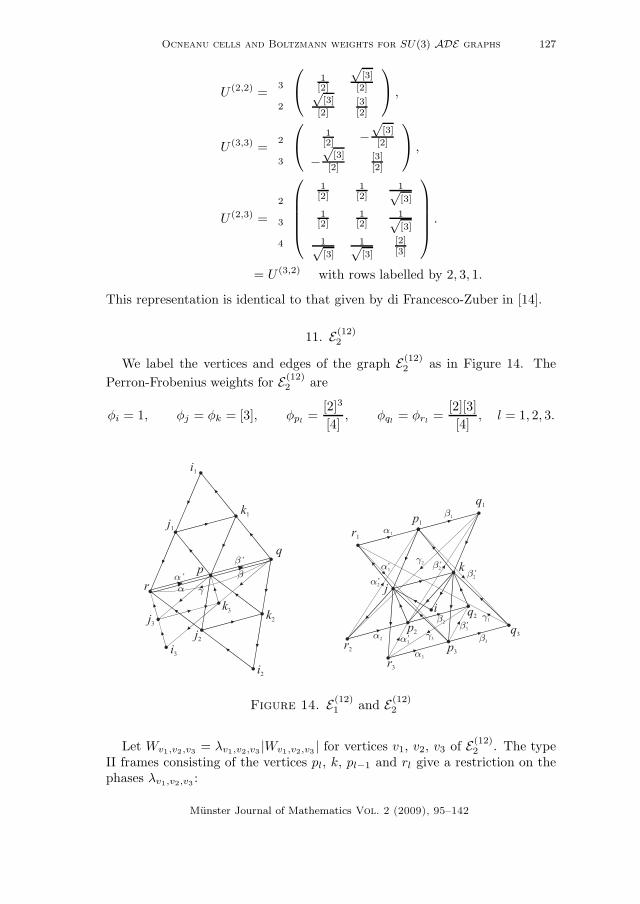
11. E(12)2
We label the vertices and edges of the graph E(12)2 as in Figure 14. The
Perron-Frobenius weights for E(12)2 are
φi = 1, φj = φk = [3], φpl=
[2]3
[4], φql
= φrl=
[2][3]
[4], l = 1, 2, 3.
Figure 14. E(12)1 and E(12)
2
Let Wv1,v2,v3 = λv1,v2,v3 |Wv1,v2,v3 | for vertices v1, v2, v3 of E(12)2 . The type
II frames consisting of the vertices pl, k, pl−1 and rl give a restriction on thephases λv1,v2,v3 :
Munster Journal of Mathematics Vol. 2 (2009), 95–142

128 David E. Evans and Mathew Pugh
0 = φ−1ql−1
Wpl−1,ql−1,rlWpl−1,ql−1,kWpl,ql−1,kWpl,ql−1,rl
+ φ−1j Wpl−1,j,rl
Wpl−1,j,kWpl,j,kWpl,j,rl
=
√[2]9[3]3
[4]5λpl−1,ql−1,rl
λpl,ql−1,kλpl−1,ql−1,kλpl,ql−1,rl
+
√[2]9[3]3
[4]5λpl−1,j,rl
λpl,j,kλpl−1,j,kλpl,j,rl,
so we have, for l = 1, 2, 3,(40)
λpl−1,ql−1,rlλpl,ql−1,kλpl−1,ql−1,kλpl,ql−1,rl
= −λpl−1,j,rlλpl,j,kλpl−1,j,kλpl,j,rl
.
Then there are two solutions W+, W− for the cell system for E(12)2 .
Theorem 11.1. Every solution for the cells of E(12)2 is either equivalent to the
solution W+ or the inequivalent conjugate solution W−, given by
W±i,j,k =
√[2][3], W±
pl,j,k=
[2]√
[3]√[4]
,
W±pl,ql−1,rl
=
√[2]
3
[4]
√[2]2 ±
√[2][4], W±
pl,ql,rl+1= −
√[2]
3
[4]
√[2]2 ∓
√[2][4],
W±pl,ql,k
= W±pl,j,rl+1
=
√[2]
3
[4]
√[2][4] ±
√[2][4],
W±pl,ql−1,k = W±
pl,j,rl=
√[2]
3
[4]
√[2][4] ∓
√[2][4],
for l = 1, 2, 3.
Proof. Let W ♯ be another solution for the cells of E(12)2 , which must be given
by W ♯v1,v2,v3
= λ♯v1,v2,v3
|W+v1,v2,v3
| where the λ♯’s satisfy the condition (40).
We need to find unitaries uv1,v2 ∈ T, for v1, v2 vertices of E(12)2 , such that
upl,qluql,rl+1
url+1,plλ♯
pl,ql,rl+1= −1, l = 1, 2, 3, and uv1,v2uv2,v3uv3,v1λ
♯v1,v2,v3
=
1 for all other triangles △v1,v2,v3 on E(12)2 . We make the following choices:
uj,k = uk,i = uj,rl= uql,k = url+1,pl
= 1, ui,j = λ♯i,j,k, upl,j = λ♯
pl,j,rl+1,
uk,pl= λ♯
pl,j,rl+1λ♯
pl,j,k, url,pl
= λ♯pl,j,rl+1
λ♯pl,j,rl
, upl,ql= λ♯
pl,j,kλ♯
pl,ql,kλ♯
pl,j,rl+1,
upl,ql−1= λ♯
pl,j,kλ♯
pl,ql−1,kλ♯pl,j,rl+1
, uql,rl+1= −λ♯
pl,j,rl+1λ♯
pl,ql,kλ♯
pl,j,kλ♯
pl,j,rl+1,
for l = 1, 2, 3.Similarly, for any solution W ♯♯ with |W ♯♯
v1,v2,v3| = |W−
v1,v2,v3|.
The solutions W+ and W− are not equivalent since |W+| 6= |W−|, and there
are no double edges on E(12)2 . We remark that the complex conjugate solutions
W± are equivalent to the solutions W∓: we choose a family of unitaries whichsatisfy (10) by uil,jl
= ujl,kl= ukl,il
= up,jl= ujl,r = uq,kl
= ukl,p = 1,
Munster Journal of Mathematics Vol. 2 (2009), 95–142

Ocneanu cells and Boltzmann weights for SU(3) ADE graphs 129
uq,r = −1, and 2 × 2 unitary matrices uα = uβ = u where u is given byu(i, j) = 1 − δi,j . �
For E(12)2 , the cells W+ above give the following representation of the Hecke
algebra, where l = 1, 2, 3 (mod 3):
U (i,k) = U (j,i) = [2],
U (k,j) =i
pl
[2][3]
√[2]3
[3]√
[4]√[2]3
[3]√
[4]
[2]2
[3][4]
,
U (rl,j) =pl−1
pl
[2]2([2][4]+√
[2][4])
[3]2[4]
√[2]3√[3][4]√
[2]3√[3][4]
[2]2([2][4]−√
[2][4])
[3]2[4]
,
= U (k,ql) with rows labelled by p,pl+1,
U (ql,pl) =k
rl+1
[2][4]+√
[2][4]
[2][3]
−
q[2][4]−
√[2][4]
[2]√
[3]
−
q[2][4]−
√[2][4]
[2]√
[3]
[2]2−√
[2][4]
[2][3]
,
= U (pl,rl+1) with rows labelled by j, ql,
U (pl,rl) =j
ql−1
[2][4]−√
[2][4]
[2][3]
q[2][4]−
√[2][4]
[2]√
[3]q[2][4]−
√[2][4]
[2]√
[3]
[2]2+√
[2][4]
[2][3]
,
= U (ql−1,pl) with rows labelled by k, rl,
U (rl+1,ql) =pl
pl+1
[2]([2]2−√
[2][4])
[3]2−[2]√
[6]
−[2]√[6]
[2]([2]2+√
[2][4])
[3]2
,
U (pl,k) =
j
ql−1
ql
1[2]
q[2][4]−
√[2][4]√
[2][3][4]
q[2][4]+
√[2][4]√
[2][3][4]q[2][4]−
√[2][4]√
[2][3][4]
[2][4]−√
[2][4]
[3][4]
√[6]√
[3][4]q[2][4]+
√[2][4]√
[2][3][4]
√[6]√
[3][4]
[2][4]+√
[2][4]
[3][4]
.
12. E(12)1
For the graph E(12)1 (illustrated in Figure 14), we will use the notation
W(1)v1,v2,v3 for the cell of the triangle △v1,v2,v3 where there are no double edges
between any of the vertices v1, v2, v3. For triangles that involve the doubleedges α, α′ or β, β′ we will specify which of the double edges is used by the
Munster Journal of Mathematics Vol. 2 (2009), 95–142
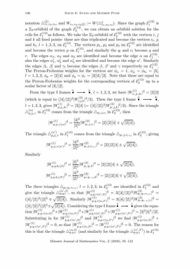
130 David E. Evans and Mathew Pugh
notation △(ξ)v1,v2,v3 , and Wv1,v2,v3(ξ) := W (△ξ
v1,v2,v3). Since the graph E(12)
1 is
a Z3-orbifold of the graph E(12)2 , we can obtain an orbifold solution for the
cells for E(12)1 as follows. We take the Z3-orbifold of E(12)
2 with the vertices i, jand k all fixed points- these are thus triplicated and become the vertices il, jl
and kl, l = 1, 2, 3, on E(12)1 . The vertices p1, p2 and p3 on E(12)
2 are identified
and become the vertex p on E(12)1 , and similarly the ql and rl become q and
r. The edges α1, α2 and α3 are identified and become the edge α on E(12)1 ,
also the edges α′1, α′
2 and α′3 are identified and become the edge α′. Similarly
the edges βl, β′l and γl become the edges β, β′ and γ respectively on E(12)
1 .The Perron-Frobenius weights for the vertices are φil
= 1, φjl= φkl
= [3],l = 1, 2, 3, φp = [2][4] and φq = φr = [3][4]/[2]. Note that these are equal to
the Perron-Frobenius weights for the corresponding vertices of E(12)2 up to a
scalar factor of [4]/[2].
From the type I framesil• -
jl•, l = 1, 2, 3, we have |W (1)il,jl,kl
|2 = [2][3]
(which is equal to ([4]/[2])2|W (2)i,j,k|2/3). Then the type I frame
jl• -kl• ,
l = 1, 2, 3, gives |W (1)p,jl,kl
|2 = [3][4] (= ([4]/[2])2|W (2)pl,j,k
|2/3). Since the triangle
△(α)p,jl,r
in E(12)1 comes from the triangle △pl,j,rl
in E(12)2 , then
|W (1)p,jl,r(α)|
2 =[4]2
[2]2|W (2)
pl,j,rl|2 = [2]([2][4]∓
√[2][4]).
The triangle △(α′)p,jl,r
in E(12)1 comes from the triangle △pl,j,rl+1
in E(12)2 , giving
|W (1)p,jl,r(α′)|2 =
[4]2
[2]2|W (2)
pl,j,rl+1|2 = [2]([2][4] ±
√[2][4]).
Similarly
|W (1)p,q,kl(β)|
2 =[4]2
[2]2|W (2)
pl,ql,k|2 = [2]([2][4] ±
√[2][4]),
|W (1)p,q,kl(β′)|2 =
[4]2
[2]2|W (2)
pl,ql−1,k|2 = [2]([2][4]∓√
[2][4]).
The three triangles △pl,ql,rl+1, l = 1, 2, 3, in E(12)
2 are identified in E(12)1 and
give the triangle △(α′,β)p,q,r , so that |W (1)
p,q,r(α′,β)|2 = 3([4]/[2])2|W (2)pl,ql,rl+1 |2 =
([4]/[2])2([2]2 ∓√
[2][4]). Similarly |W (1)p,q,r(α,β′)|2 = 3([4]/[2])2|W (2)
pl,ql−1,rl|2 =
([4]/[2])2([2]2±√
[2][4]). Considering the type I frameq• -
r• gives the equa-
tion |W (1)p,q,r(α,β)|2+|W (1)
p,q,r(α,β′)|2+|W (1)p,q,r(α′,β)|2+|W (1)
p,q,r(α′,β′)|2 = [3]2[4]2/[2].
Substituting in for |W (1)p,q,r(α′,β)|2 and |W (1)
p,q,r(α,β′)|2 we find |W (1)p,q,r(α,β)|2 +
|W (1)p,q,r(α′,β′)|2 = 0, so that |W (1)
p,q,r(α,β)|2 = |W (1)p,q,r(α′,β′)|2 = 0. The reason for
this is that the triangle △(α,β)p,q,r (and similarly for the triangle △(α′,β′)
p,q,r ) in E(12)1
Munster Journal of Mathematics Vol. 2 (2009), 95–142

Ocneanu cells and Boltzmann weights for SU(3) ADE graphs 131
comes from the paths pl- ql
- rl+1- pl+1 in E(12)
2 , which do notform a closed triangle.
From the type I framesr• -
-p• and
p• --
q•, we obtain the equations
λ1(α)λ1(α′) + λ2(α)λ2(α′) + λ3(α)λ3(α′) = 0,(41)
λ1(β)λ1(β′) + λ2(β)λ2(β′) + λ3(β)λ3(β′) = 0,(42)
where Wp,jl,r(ξ) = λl(ξ)|Wp,jl,r(ξ)|, for ξ ∈ {α, α′, β, β′}, l = 1, 2, 3. Anotherrestriction on the choice of phase is found by considering the type II framesjl• -
r• �jm• , for l 6= m, Re(λl(α)λm(α′)λl(α′)λm(α)) = −1/2, and
similarly for the type II frameskl• -
p• �km• , l 6= m, giving
λl(α)λm(α′)λl(α′)λm(α) = −1
2+ εl,m
√3
2i,(43)
λl(β)λm(β′)λl(β′)λm(β) = −1
2+ ε′l,m
√3
2i,(44)
where εl,m, ε′l,m ∈ {±1}. Lastly, from the type II frame consisting of the
vertices jl, kl, q and r (l = 1, 2, 3) we have
(45) λl(α)λl(β′)λl(α′)λl(β) = −λ(αβ′)λ(α′β),
where Wp,q,r(ξ1,ξ2) = λ(ξ1,ξ2)|Wp,q,r(ξ1,ξ2)|, for ξ1 ∈ {α, α′}, ξ2 ∈ {β, β′}, l =1, 2, 3. Then for l 6= m,
λl(α)λm(α′)λl(α′)λm(α) = λl(β)λm(β′)λl(β′)λm(β),
and, from (43) and (44) we find εl,m = ε′l,m. Substituting in for λl(α)λl(α′)
from (43) into (41), we see that εl,l+1 = εm,m+1 for all l, m = 1, 2, 3, and thatεl,l−1 = −εl,l+1. Then the restrictions for the choice of phase are (45) and(46)
λl(α)λl+1(α′)λl(α′)λl+1(α) = λl(β)λl+1(β′)λl(β′)λl+1(β) = −1
2+ ε
√3
2i = eε 2πi
3 ,
where ε ∈ {±1}.Then we have obtained two orbifold solutions for the cell system for E(12)
1 :W+, W−.
Theorem 12.1. The following solutions W+, W− for the cells of E(12)1 are
inequivalent:
W±il,jl,kl
=√
[2][3], W±p,jl,kl
=√
[3][4],
W±p,jl,r(α) = ǫl
√[2]
√[2][4]±
√[2][4], W±
p,jl,r(α′) = ǫl
√[2]
√[2][4] ∓
√[2][4],
W±p,q,kl(β) = ǫl
√[2]
√[2][4]∓
√[2][4], W±
p,q,kl(β′) = ǫl
√[2]
√[2][4] ±
√[2][4],
W±p,q,r(αβ′) =
[4]√[2]
√[2]2 ∓
√[2][4], W±
p,q,r(α′β) = − [4]√[2]
√[2]2 ±
√[2][4],
W±p,q,r(αβ) = W±
p,q,r(α′β′) = 0,
Munster Journal of Mathematics Vol. 2 (2009), 95–142

132 David E. Evans and Mathew Pugh
for l = 1, 2, 3, where ǫ1 = 1 and ǫ2 = e2πi/3 = ǫ3.
Proof. The solutions W+, W− are not equivalent, as can be seen by considering(10) for the triangle △p,jl,r. We have the following two equations, for l = 1, 2, 3:
W+p,jl,r(α) = up,jl
ujl,r
(uα(α, α)W−
p,jl ,r(α) + uα(α, α′)W−p,jl ,r(α′)
),
W+p,jl,r(α′) = up,jl
ujl,r
(uα(α′, α)W−
p,jl,r(α) + uα(α′, α′)W−p,jl,r(α′)
).
So we require up,jl, ujl,r ∈ T and a 2 × 2 unitary matrix uα such that, for
l = 1, 2, 3,
ǫl
√[2]x+ = up,jl
ujl,r
(uα(α, α)ǫl
√[2]x− + uα(α, α′)ǫl
√[2]x+
),(47)
ǫl
√[2]x− = up,jl
ujl,r
(uα(α′, α)ǫl
√[2] x− + uα(α′, α′)ǫl
√[2]x+
).(48)
where x± =√
[2][4] ±√
[2][4]. Equation (47) must hold for each l = 1, 2, 3.
On the left hand side we have ǫl, hence we require uα(α, α′) = 0 becauseuα does not depend on l, and the difference in phase between ǫl and ǫl is 0,e−2πi/3, e2πi/3 respectively for l = 1, 2, 3 respectively. This difference in phasefor each l cannot come from up,jl
ujl,r (although up,jl, ujl,r do depend on l)
since in (48) the difference in phase is now 0, e2πi/3, e−2πi/3 respectively forl = 1, 2, 3 respectively, so we would need up,jl
ujl,r to take care of the phasedifference here, not up,jl
ujl,r. Then we have uα(α, α) = up,jlujl,r x+/x−, and
similarly uα(α′, α) = 0 and uα(α′, α′) = up,jlujl,r x−/x+. But now uα is not
unitary. �
For E(12)1 , the cells W+ above give the following representation of the Hecke
algebra, where l = 1, 2, 3 (mod 3):
U (il,kl) = U (jl,il) = [2],
U (kl,jl) =il
p
[2][3]
√[2][4]
[3]√[2][4]
[3][4][3]
,
U (r,jl) =p(α)
p(α′)
[2]2([2][4]+√
[2][4])
[3]2[4]
ǫl
√[2]3√
[3][4]
ǫl
√[2]3√
[3][4]
[2]2([2][4]−√
[2][4])
[3]2[4]
= U (kl,q) with rows labelled by p(β′), p(β),
U (jl,p) =
kl
r(α)
r(α′)
1[2]
ǫl
q[2][4]+
√[2][4]√
[2][3][4]
ǫl
q[2][4]−
√[2][4]√
[2][3][4]
ǫl
q[2][4]+
√[2][4]√
[2][3][4]
[2][4]+√
[2][4]
[3][4]
ǫl
√[6]√
[3][4]
ǫl
q[2][4]−
√[2][4]√
[2][3][4]
ǫl
√[6]√
[3][4]
[2][4]−√
[2][4]
[3][4]
= U (p,kl) with rows labelled by jl, q(β′), q(β),
Munster Journal of Mathematics Vol. 2 (2009), 95–142
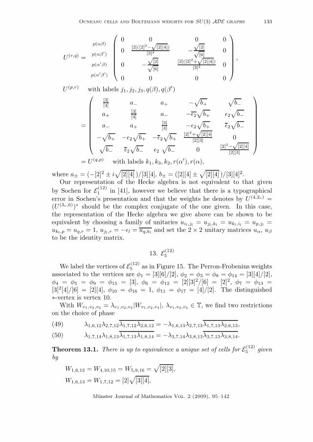
Ocneanu cells and Boltzmann weights for SU(3) ADE graphs 133
U (r,q) =
p(αβ)
p(αβ′)
p(α′β)
p(α′β′)
0 0 0 0
0[2]([2]2−
√[2][4])
[3]2 −√
[2]√[6]
0
0 −√
[2]√[6]
[2]([2]2+√
[2][4])
[3]2 0
0 0 0 0
,
U (p,r) with labels j1, j2, j3, q(β), q(β′)
=
[3][4] a− a+ −
√b+
√b−
a+[3][4] a− −ǫ2
√b+ ǫ2
√b−
a− a+[3][4] −ǫ2
√b+ ǫ2
√b−
−√
b+ −ǫ2√
b+ −ǫ2√
b+[2]2+
√[2][4]
[2][3] 0√
b− ǫ2√
b− ǫ2√
b− 0[2]2−
√[2][4]
[2][3]
= U (q,p) with labels k1, k3, k2, r(α′), r(α),
where a± = (−[2]2 ± i√
[2][4] )/[3][4], b± = ([2][4] ±√
[2][4] )/[3][4]2.Our representation of the Hecke algebra is not equivalent to that given
by Sochen for E(12)1 in [41], however we believe that there is a typographical
error in Sochen’s presentation and that the weights he denotes by U (4,2r) =(U (3r ,6))∗ should be the complex conjugate of the one given. In this case,the representation of the Hecke algebra we give above can be shown to beequivalent by choosing a family of unitaries uil,jl
= ujl,kl= ukl,il
= up,jl=
ukl,p = uq,r = 1, ujl,r = −ǫl = uq,kland set the 2 × 2 unitary matrices uα, uβ
to be the identity matrix.
13. E(12)5
We label the vertices of E(12)5 as in Figure 15. The Perron-Frobenius weights
associated to the vertices are φ1 = [3][6]/[2], φ2 = φ3 = φ8 = φ14 = [3][4]/[2],φ4 = φ5 = φ9 = φ15 = [3], φ6 = φ12 = [2][3]2/[6] = [2]2, φ7 = φ13 =[3]2[4]/[6] = [2][4], φ10 = φ16 = 1, φ11 = φ17 = [4]/[2]. The distinguished∗-vertex is vertex 10.
With Wv1,v2,v3 = λv1,v2,v3 |Wv1,v2,v3 |, λv1,v2,v3 ∈ T, we find two restrictionson the choice of phase
λ1,6,12λ2,7,12λ1,7,12λ2,6,12 = −λ1,6,13λ2,7,13λ1,7,13λ2,6,13,(49)
λ1,7,14λ1,8,13λ1,7,13λ1,8,14 = −λ3,7,14λ3,8,13λ3,7,13λ3,8,14.(50)
Theorem 13.1. There is up to equivalence a unique set of cells for E(12)5 given
by
W1,6,12 = W4,10,15 = W5,9,16 =√
[2][3],
W1,6,13 = W1,7,12 = [2]√
[3][4],
Munster Journal of Mathematics Vol. 2 (2009), 95–142

134 David E. Evans and Mathew Pugh
Figure 15. Labelled graph E(12)5
W1,7,13 = W3,7,14 = W3,8,13 = W3,8,17 = W3,11,14 = W2,7,15 = W2,9,13
= W4,7,14 = W5,8,13 =[4]√
[3]√[2]
,
W1,8,14 =[4]√
[3][6]√[2]
, W1,7,14 = W1,8,13 =
√[3][4][6]√
[2],
W2,6,12 = [4]√
[2], W2,6,13 = W2,7,12 = [2]√
[4],
W2,7,13 = −[4]√
[2], W3,7,13 = −[4]√
[6],
W3,8,14 =[4]√
[6]
[2], W4,7,15 = W5,9,13 =
√[3][4].
Proof. Let W ♯ be any other solution for the cells of E(12)5 . Then we have
W ♯v1,v2,v3
= λ♯v1,v2,v3
|Wv1,v2,v3 |, where the λ♯’s satisfy the conditions (49) and
(50). We need to find unitaries uv1,v2 ∈ T which satisfy u7,13u13,2u2,7λ♯2,7,13 =
−1, u7,13u13,3u3,7λ♯3,7,13 = −1 and uv1,v2uv2,v3uv3,v1λ
♯v1,v2,v3
= 1 for all other
triangles △v1,v2,v3 on E(12)5 . We set u2,7 = u2,9 = u3,8 = u3,11 = u6,13 = u7,13 =
u7,14 = u8,13 = u8,17 = u9,16 = u10,15 = u12,1 = u12,2 = u13,5 = u14,7 =
u15,2 = 1, u5,8 = λ♯5,8,13, u7,12 = λ♯
2,7,12, u7,15 = λ♯2,7,15, u11,14 = −λ♯
3,11,14,
u13,1 = λ♯1,6,13, u13,2 = −λ♯
2,7,13, u13,3 = λ♯3,8,13, u14,4 = λ♯
4,7,14, u17,3 =
λ♯3,8,17, u1,7 = λ♯
2,7,12λ♯1,7,12, u2,6 = −λ♯
2,7,13λ♯2,6,13, u3,7 = −λ♯
3,8,13λ♯3,7,13,
u9,13 = −λ♯2,7,13λ
♯2,9,13, u15,4 = λ♯
2,7,15λ♯4,7,15, u4,10 = λ♯
4,7,15λ♯2,7,15λ
♯4,10,15,
u5,9 = −λ♯2,9,13λ
♯2,7,13λ
♯5,9,13, u6,12 = −λ♯
2,6,13λ♯2,6,12λ
♯2,7,13,
u14,1 = λ♯1,7,12λ
♯1,7,14λ
♯2,7,12, u14,3 = −λ♯
3,7,13λ♯3,7,14λ
♯3,8,13,
Munster Journal of Mathematics Vol. 2 (2009), 95–142

Ocneanu cells and Boltzmann weights for SU(3) ADE graphs 135
u1,6 = −λ♯2,6,12λ
♯2,7,13λ
♯1,6,12λ
♯2,6,13, u1,8 = λ♯
1,7,12λ♯1,7,13λ
♯1,8,13λ
♯2,7,12,
u8,14 = λ♯1,7,14λ
♯1,8,13λ
♯1,7,13λ
♯1,8,14 and u16,5 = −λ♯
2,7,13λ♯5,9,13λ
♯2,9,13λ
♯5,9,16. �
For E(12)5 , we have the following representation of the Hecke algebra:
U (5,16) = U (16,9) = U (10,4) = U (15,10) = [2],
U (3,17) = U (17,8) = U (11,3) = U (14,11) =[2]
[4],
U (2,15) = U (4,14) = U (8,5) = U (9,2) =[4]
[3],
U (14,8) =3
1
1[2]
√[3]√[2]√
[3]√[2]
[3]
U (12,7) =2
1
1[2]
√[3]
[2]√[3]
[2][3][2]
= U (13,6) with rows labelled by 2, 1
U (3,13) =8
7
1[2] −
√[3]
[2]
−√
[3]
[2][3][2]
= U (7,3) with rows labelled by 14, 13
U (5,13) =9
8
1[2]
√[4]√[2]3√
[4]√[2]3
[4][2]2
= U (13,9) with labels 5,2
= U (7,4) with labels 15,14 = U (15,7) with labels 4,2
U (2,12) =7
6
[2][3]
√[2][4]
[3]√[2][4]
[3][4][3]
= U (6,2) with labels 13,12
= U (4,15) with labels 10,7 = U (9,5) with labels 16,13
U (1,14) =7
8
[2][3]
[2]√
[4]
[3]
[2]√
[4]
[3][2][4][3]
= U (8,1) with labels 13,14
U (12,6) =1
2
[3][2]3
[4]√
[3]
[2]3
[4]√
[3]
[2]3[4]2
[2]3
U (1,12) =6
7
1[6]
√[2][4]
[6]√[2][4]
[6][2][4][6]
= U (6,1) with labels 12,13
Munster Journal of Mathematics Vol. 2 (2009), 95–142

136 David E. Evans and Mathew Pugh
U (13,8) =
5
3
1
1[2]
1[2]
√[6]
[2]√
[4]
1[2]
1[2]
√[6]
[2]√
[4]√[6]
[2]√
[4]
√[6]
[2]√
[4]
[6][2][4]
= U (14,7) with labels 4,3,1
U (3,14) =
8
7
11
1[2]
1√[3]
1√[3]
1√[3]
[2][3]
[2][3]
1√[3]
[2][3]
[2][3]
= U (8,3) with labels 14,13,17
U (2,13) =
9
7
6
1[2] − 1√
[3]
√[2]√
[3][4]
− 1√[3]
[2][3] −
√[2]3
[3]√
[4]√[2]√
[3][4]−
√[2]3
[3]√
[4]
[2]2
[3][4]
= U (7,2) with labels 15,13,12,
U (1,13) =
8
7
6
1[2]
√[4]
[2]√
[6]
√[2]3√[6]√
[4]
[2]√
[6]
[4][2][6]
√[2]3[4]
[6]√[2]3√[6]
√[2]3[4]
[6][2]2
[6]
= U (7,1) with labels 14,13,12
U (13,7) =
2
3
1
1[2]
√[6]√[2]3
−√
[3]
[2]2√[6]√[2]3
[6][2]2 −
√[3][6]√[2]5
−√
[3]
[2]2 −√
[3][6]√[2]5
[3][2]3
.
14. E(24)
We label the vertices of the graph E(24) as in Figure 16. The Perron-Frobenius weights are: φ1 = φ8 = 1, φ2 = φ7 = [2][4], φ3 = φ6 = [4][5]/[2],φ4 = φ5 = [4][7]/[2], φ9 = φ16 = φ17 = φ24 = [3], φ10 = φ15 = φ18 = φ23 =[3][4]/[2], φ11 = φ14 = φ19 = φ22 = [3][5] and φ12 = φ13 = φ20 = φ21 = [9].With [a] = [a]q, q = eiπ/24, we have the relation [4]2 = [2][10].
The following cells follow from the A case: |W1,9,17|2 = |W8,16,24|2 = [2][3],|W2,9,17|2 = |W7,16,24|2 = [3][4], |W2,9,18|2 = |W2,10,17|2 = |W7,15,24|2 =|W7,16,23|2 = [3]2[4], |W2,10,19|2 = |W2,11,18|2 = |W7,14,23|2 = |W7,15,22|2 =[3][4][5], |W2,11,19|2 = |W7,14,22|2 = [3]2[4][5] and |W3,10,19|2 = |W3,14,23|2 =|W6,11,18|2 = |W6,15,22|2 = [3][4]2[5]/[2].
Munster Journal of Mathematics Vol. 2 (2009), 95–142
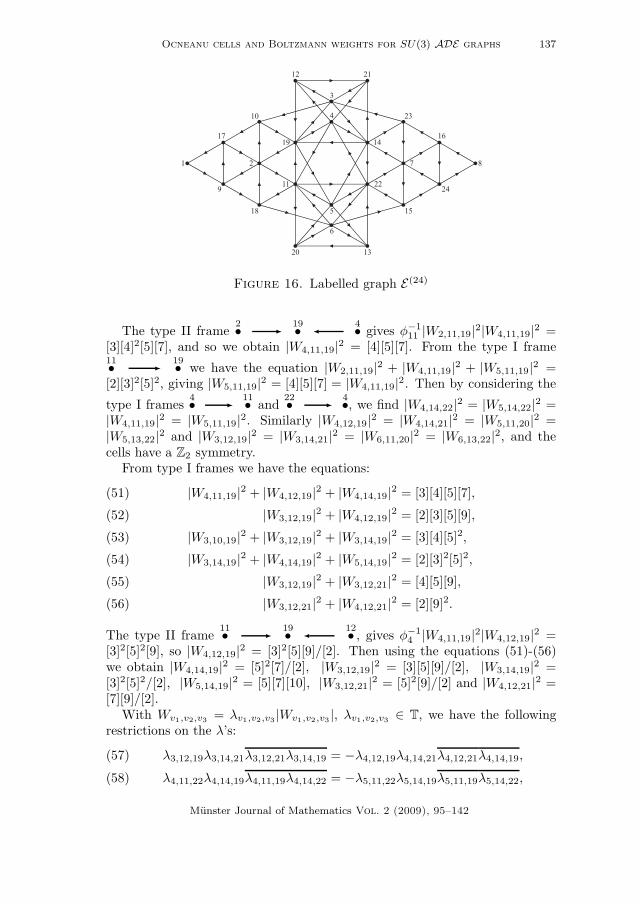
Ocneanu cells and Boltzmann weights for SU(3) ADE graphs 137
Figure 16. Labelled graph E(24)
The type II frame2• -
19• �4• gives φ−1
11 |W2,11,19|2|W4,11,19|2 =[3][4]2[5][7], and so we obtain |W4,11,19|2 = [4][5][7]. From the type I frame11• -
19• we have the equation |W2,11,19|2 + |W4,11,19|2 + |W5,11,19|2 =[2][3]2[5]2, giving |W5,11,19|2 = [4][5][7] = |W4,11,19|2. Then by considering the
type I frames4• -
11• and22• -
4•, we find |W4,14,22|2 = |W5,14,22|2 =|W4,11,19|2 = |W5,11,19|2. Similarly |W4,12,19|2 = |W4,14,21|2 = |W5,11,20|2 =|W5,13,22|2 and |W3,12,19|2 = |W3,14,21|2 = |W6,11,20|2 = |W6,13,22|2, and thecells have a Z2 symmetry.
From type I frames we have the equations:
|W4,11,19|2 + |W4,12,19|2 + |W4,14,19|2 = [3][4][5][7],(51)
|W3,12,19|2 + |W4,12,19|2 = [2][3][5][9],(52)
|W3,10,19|2 + |W3,12,19|2 + |W3,14,19|2 = [3][4][5]2,(53)
|W3,14,19|2 + |W4,14,19|2 + |W5,14,19|2 = [2][3]2[5]2,(54)
|W3,12,19|2 + |W3,12,21|2 = [4][5][9],(55)
|W3,12,21|2 + |W4,12,21|2 = [2][9]2.(56)
The type II frame11• -
19• �12• , gives φ−1
4 |W4,11,19|2|W4,12,19|2 =[3]2[5]2[9], so |W4,12,19|2 = [3]2[5][9]/[2]. Then using the equations (51)-(56)we obtain |W4,14,19|2 = [5]2[7]/[2], |W3,12,19|2 = [3][5][9]/[2], |W3,14,19|2 =[3]2[5]2/[2], |W5,14,19|2 = [5][7][10], |W3,12,21|2 = [5]2[9]/[2] and |W4,12,21|2 =[7][9]/[2].
With Wv1,v2,v3 = λv1,v2,v3 |Wv1,v2,v3 |, λv1,v2,v3 ∈ T, we have the followingrestrictions on the λ’s:
λ3,12,19λ3,14,21λ3,12,21λ3,14,19 = −λ4,12,19λ4,14,21λ4,12,21λ4,14,19,(57)
λ4,11,22λ4,14,19λ4,11,19λ4,14,22 = −λ5,11,22λ5,14,19λ5,11,19λ5,14,22,(58)
Munster Journal of Mathematics Vol. 2 (2009), 95–142

138 David E. Evans and Mathew Pugh
λ5,11,20λ5,13,22λ5,11,22λ5,13,20 = −λ6,11,20λ6,13,22λ6,11,22λ6,13,20.(59)
Theorem 14.1. There is up to equivalence a unique set of cells for E(24) givenby
W1,9,17 = W8,16,24 =√
[2][3], W2,9,17 = W7,16,24 =√
[3][4],
W2,9,18 = W2,10,17 = W7,15,24 = W7,16,23 = [3]√
[4],
W2,10,19 = W2,11,18 = W7,14,23 = W7,15,22 =√
[3][4][5],
W2,11,19 = W7,14,22 = [3]√
[4][5],
W3,10,19 = W3,14,23 = W6,11,18 = W6,15,22 =[4]√
[3][5]√[2]
,
W4,11,19 = W4,14,22 = W5,11,19 = W5,14,22 =√
[4][5][7],
W4,12,19 = W4,14,21 = W5,11,20 = W5,13,22 =[3]√
[5][9]√[2]
,
W3,12,19 = W3,14,21 = W6,11,20 = W6,13,22 =
√[3][5][9]√
[2],
W3,14,19 = W6,11,22 =[3][5]√
[2], W4,14,19 = W5,11,22 =
[5]√
[7]√[2]
,
W5,14,19 =√
[5][7][10], W4,11,22 = −√
[5][7][10],
W3,12,21 = W6,13,20 = − [5]√
[9]√[2]
, W4,12,21 = W5,13,20 =
√[7][9]√[2]
.
Proof. Let W ♯ be any solution for the cells of E(24). Then W ♯v1,v2,v3
=
λ♯v1,v2,v3
|Wv1,v2,v3 |, where the λ♯’s satisfy the conditions (57), (58) and (59).
We need to find unitaries uv1,v2 ∈ T such that u12,21u21,3u3,12λ♯3,12,21 = −1,
u13,20u20,6u6,13λ♯6,13,20 = −1, u11,22u22,4u4,11λ
♯4,11,22 = −1, and for all other
triangles △v1,v2,v3 on E(24) we require uv1,v2uv2,v3uv3,v1λ♯v1,v2,v3
= 1. We makethe following choices for the uv1,v2 :
u3,12 = u3,14 = u4,11 = u5,13 = u5,14 = u11,20
= u14,19 = u20,6 = u21,3 = u21,4 = u22,6 = 1,
u12,21 = −λ♯3,12,21, u14,21 = λ♯
3,14,21, u19,3 = λ♯3,14,19, u19,5 = −λ♯
5,14,19,
u4,12 = −λ♯3,12,21λ
♯4,12,21, u4,14 = λ♯
3,14,21λ♯4,14,21, u6,11 = λ♯
5,14,22λ♯6,11,20,
u12,19 = λ♯3,14,19λ
♯3,12,19, u11,22 = λ♯
6,11,20λ♯5,14,22λ
♯6,11,22,
u19,4 = λ♯4,14,21λ
♯3,14,21λ
♯4,14,19, u22,4 = −λ♯
5,14,22λ♯6,11,22λ
♯4,11,22λ
♯6,11,20,
u5,11 = −λ♯4,11,22λ
♯4,14,21λ
♯5,14,22λ
♯3,14,21λ
♯4,14,22λ
♯5,11,22,
u11,19 = −λ♯3,12,21λ
♯3,14,19λ
♯4,12,19λ
♯3,12,19λ
♯4,11,19λ
♯4,12,21,
Munster Journal of Mathematics Vol. 2 (2009), 95–142
Ocneanu cells and Boltzmann weights for SU(3) ADE graphs 139
u20,5 = −λ♯3,14,21λ
♯4,14,22λ
♯5,11,22λ
♯4,11,22λ
♯4,14,21λ
♯5,11,20,
u22,5 = −λ♯3,14,21λ
♯4,14,22λ
♯6,11,22λ
♯4,11,22λ
♯4,14,21λ
♯6,11,20,
u13,22 = −λ♯4,11,22λ
♯4,14,21λ
♯6,11,20λ
♯3,14,21λ
♯4,14,22λ
♯5,13,22λ
♯6,11,22,
u14,22 = −λ♯4,11,22λ
♯4,14,21λ
♯6,11,20λ
♯3,14,21λ
♯4,14,22λ
♯5,14,22λ
♯6,11,22,
u6,13 = −λ♯3,14,21λ
♯4,14,22λ
♯5,13,22λ
♯6,11,22λ
♯4,11,22λ
♯4,14,21λ
♯6,11,20λ
♯6,13,22,
u13,20 = λ♯4,11,22λ
♯4,14,21λ
♯6,11,20λ
♯6,13,22λ
♯3,14,21λ
♯4,14,22λ
♯5,13,22λ
♯6,11,22λ
♯6,13,20.
The uv1,v2 involving the vertices 1, 2, 7, 8, 9, 10, 15, 16, 17, 18, 23 and 24are chosen in the same way as in the proof of uniqueness of the cells for the Agraphs. �
For E(24), we have the following representation of the Hecke algebra (weomit those weights which come from the A(24) graph):
U (3,21) =12
14
[5][4] −
√[3][5]
[4]
−√
[3][5]
[4][3][4]
= U (12,3) with labels 21,19
= U (6,20) with labels 13,11 = U (13,6) with labels 20,22
U (19,12) =3
4
1[2]
√[3]
[2]√[3]
[2][3][2]
= U (21,14) with labels 3,4
= U (20,11) with labels 6,5 = U (22,13) with labels 6,5,
U (5,19) =11
14
[2][3]
√[2][4]
[3]√[2][4]
[3][4][3]
= U (14,5) with labels 22,19
U (4,22) =14
11
[2][3] −
√[2][4]
[3]
−√
[2][4]
[3][4][3]
= U (11,4) with labels 19,22,
U (20,13) =6
5
[5]2
[2][9] − [5]√
[7]
[2][9]
− [5]√
[7]
[2][9][7]
[2][9]
= U (21,12) with labels 3,4
U (4,21) =12
14
1[4]
[3]√
[5]
[4]√
[7]
[3]√
[5]
[4]√
[7]
[3]2[5][4][7]
= U (12,4) with labels 21,19
= U (5,20) with labels 13,11 = U (13,5) with labels 20,22
Munster Journal of Mathematics Vol. 2 (2009), 95–142

140 David E. Evans and Mathew Pugh
U (19,14) =
3
4
5
1[2]
√[7]
[2][3]
√[7][10]
[3]√
[2][5]√[7]
[2][3][7]
[2][3]2[7]√
[10]
[3]2√
[2][5]√[7][10]
[3]√
[2][5]
[7]√
[10]
[3]2√
[2][5]
[7][10][3]2[5]
U (22,11) =
6
5
4
1[2]
√[7]
[2][3] −√
[7][10]
[3]√
[2][5]√[7]
[2][3][7]
[2][3]2 − [7]√
[10]
[3]2√
[2][5]
−√
[7][10]
[3]√
[2][5]− [7]
√[10]
[3]2√
[2][5]
[7][10][3]2[5]
U (19,11) =
2
4
5
[4][5]
[4]√
[7]
[3][5]
[4]√
[7]
[3][5]
[4]√
[7]
[3][5][4][7][3]2[5]
[4][7][3]2[5]
[4]√
[7]
[3][5][4][7][3]2[5]
[4][7][3]2[5]
= U (22,14) with labels 7,4,5
U (3,19) =
10
14
12
[4][5]
√[3]√[5]
√[9]
[5]√[3]√[5]
[3][4]
√[3][9]
[4]√
[5]√[9]
[5]
√[3][9]
[4]√
[5]
[9][4][5]
= U (14,3) with labels 23,19,21
= U (6,22) with labels 15,11,13 = U (11,6) with labels 18,22,20
U (4,19) =
11
14
12
[2][3]
√[2][5]
[3]√
[4]
√[2][9]√[4][7]√
[2][5]
[3]√
[4]
[5][3][4]
√[5][9]
[4]√
[7]√[2][9]√[4][7]
√[5][9]
[4]√
[7]
[3][9][4][7]
= U (14,4) with labels 22,19,21 = U (5,22) with labels 14,11,13
= U (11,5) with labels 19,22,20.
The Hecke representation given above cannot be equivalent to that given bySochen in [41] for E(24) as our weights [U (14,4)]19,19, [U (14,4)]21,21, [U (11,5)]20,20,
[U (11,5)]22,22 and [U (19,11)]2,2 (as well as the corresponding weights under thereflection of the graph which sends vertices 1 �- 8) have different absolutevalues to those given by Sochen (and there are no double edges on the graph).We do not believe that there exists two inequivalent solutions for the Heckerepresentation for E(24), and that the differences must be due to typographicalerrors in [41].
Acknowledgements. This paper is based on work in [40]. The first author waspartially supported by the EU-NCG network in Non-Commutative Geometry
Munster Journal of Mathematics Vol. 2 (2009), 95–142

Ocneanu cells and Boltzmann weights for SU(3) ADE graphs 141
MRTN-CT-2006-031962, and the second author was supported by a scholarshipfrom the School of Mathematics, Cardiff University.
References
[1] E. Ardonne and K. Schoutens, Wavefunctions for topological quantum registers, Ann.Physics 322 (2007), no. 1, 201–235. MR2286783 (2008d:81276)
[2] F. A. Bais and J. K. Slingerland, Condensate-induced transitions between topologicallyordered phases, Phys. Rev. B 79 (2009), 045316 (27 pages).
[3] T. Banica and D. Bisch, Spectral measures of small index principal graphs, Comm.Math. Phys. 269 (2007), no. 1, 259–281. MR2274471 (2008f:46078)
[4] R. E. Behrend and D. E. Evans, Integrable lattice models for conjugate A(1)n , J. Phys.
A 37 (2004), no. 8, 2937–2947. MR2021644 (2004m:82027)[5] J. Bockenhauer and D. E. Evans, Modular invariants, graphs and α-induction for nets of
subfactors. I, Comm. Math. Phys. 197 (1998), no. 2, 361–386. MR1652746 (2000c:46121)[6] J. Bockenhauer and D. E. Evans, Modular invariants, graphs and α-induction for nets of
subfactors. II, Comm. Math. Phys. 200 (1999), no. 1, 57–103. MR1671970 (2000c:46122)[7] J. Bockenhauer and D. E. Evans, Modular invariants, graphs and α-induction for
nets of subfactors. III, Comm. Math. Phys. 205 (1999), no. 1, 183–228. MR1706884(2000j:46118)
[8] J. Bockenhauer and D. E. Evans, Modular invariants from subfactors: Type I couplingmatrices and intermediate subfactors, Comm. Math. Phys. 213 (2000), no. 2, 267–289.MR1785458 (2001g:46142)
[9] J. Bockenhauer, D. E. Evans and Y. Kawahigashi, On α-induction, chiral generatorsand modular invariants for subfactors, Comm. Math. Phys. 208 (1999), no. 2, 429–487.MR1729094 (2001c:81180)
[10] J. Bockenhauer, D. E. Evans and Y. Kawahigashi, Chiral structure of modular in-variants for subfactors, Comm. Math. Phys. 210 (2000), no. 3, 733–784. MR1777347(2001k:46097)
[11] A. Cappelli, C. Itzykson and J.-B. Zuber, Modular invariant partition functions in twodimensions, Nuclear Phys. B 280 (1987), no. 3, 445–465. MR0881119 (88i:81132)
[12] A. Cappelli, C. Itzykson and J.-B. Zuber, The A-D-E classification of minimal and A(1)1
conformal invariant theories, Comm. Math. Phys. 113 (1987), no. 1, 1–26. MR0918402(89b:81178)
[13] P. Di Francesco, Integrable lattice models, graphs and modular invariant conformal fieldtheories, Internat. J. Modern Phys. A 7 (1992), no. 3, 407–500. MR1142944 (93d:82027)
[14] P. Di Francesco and J.-B. Zuber, SU(N) lattice integrable models associated withgraphs, Nuclear Phys. B 338 (1990), no. 3, 602–646. MR1063590 (91i:82005)
[15] D. E. Evans, Critical phenomena, modular invariants and operator algebras, in Oper-ator algebras and mathematical physics (Constanta, 2001), 89–113, Theta, Bucharest.MR2018226 (2005e:46117)
[16] D. E. Evans and T. Gannon, Modular Invariants and Twisted Equivariant K-theory. Toappear in Commun. Number Theory Phys. arXiv:0807.3759.
[17] D. E. Evans and Y. Kawahigashi, Orbifold subfactors from Hecke algebras, Comm.Math. Phys. 165 (1994), no. 3, 445–484. MR1301620 (96c:46059)
[18] D. E. Evans and Y. Kawahigashi, Quantum symmetries on operator algebras, OxfordUniv. Press, New York, 1998. MR1642584 (99m:46148)
[19] D. E. Evans and P. R. Pinto, Subfactor realisation of modular invariants, Comm. Math.Phys. 237 (2003), no. 1-2, 309–363. MR2007185 (2005k:46166)
[20] D. E. Evans and M. Pugh, SU(3)-Goodman-de la Harpe-Jones subfactors and the re-alisation of SU(3) modular invariants. To appear in Rev. Math. Phys. arXiv:0906.4252[math.OA]
[21] D. E. Evans and M. Pugh, A2-planar algebras I. arXiv:0906.4225 [math.OA]
Munster Journal of Mathematics Vol. 2 (2009), 95–142

142 David E. Evans and Mathew Pugh
[22] D. E. Evans and M. Pugh, A2-planar algebras II: Planar modules. arXiv:0906.4311[math.OA]
[23] D. E. Evans and M. Pugh, Spectral measures and generating series for nimrep graphsin subfactor theory. To appear in Comm. Math. Phys. arXiv:0906.4314 [math.OA]
[24] D. E. Evans and M. Pugh, Spectral measures and generating series for nimrep graphsin subfactor theory II. In preparation.
[25] P. Fendley, New exactly solvable orbifold models, J. Phys. A 22 (1989), no. 21, 4633–4642. MR1022137 (91d:81092)
[26] T. Gannon, The classification of affine SU(3) modular invariant partition functions,Comm. Math. Phys. 161 (1994), no. 2, 233–263. MR1266482 (95b:81072)
[27] A. Guionnet, V. F. R. Jones and D. Shlyakhtenko, Random Matrices, Free Probability,Planar Algebras and Subfactors. Preprint 2008. arXiv:0712.2904.
[28] M. Jimbo, T. Miwa and M. Okado, Solvable lattice models whose states are dominant
integral weights of A(1)n−1, Lett. Math. Phys. 14 (1987), no. 2, 123–131. MR0908997
(89e:82017)[29] V. F. R. Jones, Index for subfactors, Invent. Math. 72 (1983), no. 1, 1–25. MR0696688
(84d:46097)[30] V. F. R. Jones, Planar algebras. I, New Zealand J. Math. (to appear)[31] L. H. Kauffman, State models and the Jones polynomial, Topology 26 (1987), no. 3,
395–407. MR0899057 (88f:57006)[32] G. Kuperberg, Spiders for rank 2 Lie algebras, Comm. Math. Phys. 180 (1996), no. 1,
109–151. MR1403861 (97f:17005)[33] G. Moore and N. Seiberg, Naturality in conformal field theory, Nuclear Phys. B 313
(1989), no. 1, 16–40. MR0984288 (90f:81119)[34] A. Ocneanu, Quantized groups, string algebras and Galois theory for algebras, in Op-
erator algebras and applications, Vol. 2, 119–172, Cambridge Univ. Press, Cambridge.MR0996454 (91k:46068)
[35] A. Ocneanu, Paths on Coxeter diagrams: from Platonic solids and singularities to mini-mal models and subfactors. (Notes recorded by S. Goto), in Lectures on operator theory,(ed. B. V. Rajarama Bhat et al.), The Fields Institute Monographs, 243–323, Amer.Math. Soc., Providence, R.I., 2000.
[36] A. Ocneanu, Higher Coxeter Systems (2000). Talk given at MSRI.http://www.msri.org/publications/ln/msri/2000/subfactors/ocneanu.
[37] A. Ocneanu, The classification of subgroups of quantum SU(N), in Quantum sym-metries in theoretical physics and mathematics (Bariloche, 2000), 133–159, Contemp.Math., 294, Amer. Math. Soc., Providence, RI. MR1907188 (2003h:81101)
[38] V. B. Petkova and J.-B. Zuber, From CFT to graphs, Nuclear Phys. B 463 (1996),no. 1, 161–193. MR1385649 (97a:81212)
[39] S. Popa, An axiomatization of the lattice of higher relative commutants of a subfactor,Invent. Math. 120 (1995), no. 3, 427–445. MR1334479 (96g:46051)
[40] M. Pugh, The Ising Model and Beyond, PhD thesis, Cardiff University, 2008.[41] N. Sochen, Integrable models through representations of the Hecke algebra, Nuclear
Phys. B 360 (1991), no. 2-3, 613–640. MR1118801 (92i:82037)[42] H. Wenzl, Hecke algebras of type An and subfactors, Invent. Math. 92 (1988), no. 2,
349–383. MR0936086 (90b:46118)
Received February 2, 2009; accepted May 25, 2009
David E. Evans and Mathew PughSchool of Mathematics, Cardiff UniversitySenghennydd Road, Cardiff, CF24 4AG, Wales, UKE-mail: {evansde,pughmj}@cardiff.ac.uk
Munster Journal of Mathematics Vol. 2 (2009), 95–142