OceanView Installation and Operation Manual - Ocean … · OceanView Installation and Operation...
118
OceanView Installation and Operation Manual For Products: OceanView Document: 000-20000-310-02-201602c
Transcript of OceanView Installation and Operation Manual - Ocean … · OceanView Installation and Operation...

OceanView Installation and Operation Manual
For Products: OceanView
Document: 000-20000-310-02-201602c

AMERICAS & WORLD HEADQUARTERS
Phone: +1 727-733-2447 Fax: +1 727-733-3962 Sales: [email protected] Orders: [email protected] Support: [email protected]
EUROPE, MIDDLE EAST & AFRICA
Phone: +31 26-319-0500 Fax: +31 26-319-0505 Email: [email protected] Germany : +49 711-341696-0
UK : +44 1865-811118 France : +33 442-386-588
ASIA
Phone: +86 21-6295-6600 Fax: +86 21-6295-6708 Email: [email protected]
Japan & Korea: +82 10-8514-3797
www.oceanoptics.com
Copyright © 2013 Ocean Optics, Inc. All rights reserved. No part of this publication may be reproduced, stored in a retrieval system, or transmitted, by any means, electronic, mechanical, photocopying, recording, or otherwise, without written permission from Ocean Optics, Inc.
Trademarks
All products and services herein are the trademarks, service marks, registered trademarks or registered service marks of their respective owners.
Limit of Liability Every effort has been made to make this manual as complete and as accurate as possible, but no warranty or fitness is implied. The information provided is on an “as is” basis. Ocean Optics, Inc. shall have neither liability nor responsibility to any person or entity with respect to any loss or damages arising from the information contained in this manual.
Ocean Optics, Inc. 830 Douglas Ave. Dunedin, FL 34698 USA Manufacturing & Logistics 4301 Metric Dr. Winter Park, FL 32792 USA
Ocean Optics Asia 666 Gubei Road Kirin Tower Suite 601B Changning District Shanghai PRC, 200336
Sales & Support Geograaf 24 6921 EW Duiven The Netherlands Manufacturing & Logistics Maybachstrasse 11 73760 Ostfildern Germany
000-20000-310-02-201602c i
Table of Contents
About This Manual ................................................................................................................... vii
Document Purpose and Intended Audience .......................................................................... vii
What’s New in this Document .............................................................................................. vii
Document Summary ............................................................................................................. vii
Product-Related Documentation ........................................................................................... vii
Chapter 1: Introduction ............................................................................ 1
Product Overview ....................................................................................................................... 1
USB Spectrometer and Device Control ...................................................................................... 1
Features ....................................................................................................................................... 2
Spectroscopic Functions ............................................................................................................. 4
Getting Updates .......................................................................................................................... 4
Chapter 2: Installation .............................................................................. 5
Overview ..................................................................................................................................... 5
OceanView Minimum System Requirements ............................................................................. 5
Installation................................................................................................................................... 5
Installing on a Windows Platform .......................................................................................... 6
Installing on a Macintosh Platform ......................................................................................... 7
Installing on a Linux Platform ................................................................................................ 8
Retrieving from a CD.............................................................................................................. 9
Product Activation .................................................................................................................... 10
Licensing ............................................................................................................................... 10
Starting Your 10 Day Free Trial ........................................................................................... 10
Using Your Product Key to Activate Your Software ........................................................... 10
Deactivating Your Product Key for Software Installation on Another Computer ................ 11
Table of Contents
ii 000-20000-300-02-201602c
Connecting Your Spectrometer................................................................................................. 11
Chapter 3: User Interface ....................................................................... 13
Launching OceanView.............................................................................................................. 13
Welcome Screen ....................................................................................................................... 13
Quick View ........................................................................................................................... 14
Spectroscopy Application Wizards ....................................................................................... 14
Load a Saved Project ............................................................................................................ 15
Restore Last Session ............................................................................................................. 15
Views ........................................................................................................................................ 16
Graph View ........................................................................................................................... 16
Schematic View .................................................................................................................... 16
Online Help ............................................................................................................................... 17
Main Window Controls............................................................................................................. 18
Creating a New Spectroscopy Application ........................................................................... 18
Opening a Project .................................................................................................................. 18
Saving a Project .................................................................................................................... 18
Removing a Project ............................................................................................................... 19
Using the Device Manager.................................................................................................... 19
Start All File Writers ............................................................................................................. 19
Control All Acquisitions ....................................................................................................... 20
Acquisition Parameter Controls ................................................................................................ 20
Main Controls Tab ................................................................................................................ 22
Flame Direct-Attach Accessories ......................................................................................... 26
Add/Remove Controls Tab ................................................................................................... 28
GPIO Function ...................................................................................................................... 28
Graph View Controls ................................................................................................................ 29
Configure Graph Saving ....................................................................................................... 31
Saved Data Panel .................................................................................................................. 33
Graph Layer Options Window .............................................................................................. 34
Menus ........................................................................................................................................ 39
File Menu .............................................................................................................................. 39
Table of Contents
000-20000-310-02-201602c iii
Window Menu ...................................................................................................................... 42
Help Menu ............................................................................................................................ 46
Chapter 4: Wizards ................................................................................. 47
Overview ................................................................................................................................... 47
Select Data Source Wizard ....................................................................................................... 47
Set Acquisition Parameters Wizard .......................................................................................... 47
Select Spectroscopy Wizard ..................................................................................................... 48
Peak Metrics Wizard ............................................................................................................. 56
Strip Chart Wizard ................................................................................................................ 58
Splicing Spectral Data............................................................................................................... 60
Chpater 5: Schematic View .................................................................... 63
Overview ................................................................................................................................... 63
Using the Schematic View ........................................................................................................ 63
Spectrometers ........................................................................................................................ 63
Acquisitions .......................................................................................................................... 64
Displaying the Schematic View ................................................................................................ 64
Sizing the Schematic View ................................................................................................... 64
Schematic Icons ........................................................................................................................ 69
Devices .................................................................................................................................. 69
Nodes .................................................................................................................................... 70
Creating a Schematic View ....................................................................................................... 70
Order of Operations .............................................................................................................. 73
Icon Definitions ........................................................................................................................ 73
Absolute Value (Abs) ........................................................................................................... 73
Acquisition (Acquire) ........................................................................................................... 74
Add Color View (Color) ....................................................................................................... 74
Add Graph View (View) ....................................................................................................... 74
Add Scalar View (Scalar) ..................................................................................................... 75
Add (Add) ............................................................................................................................. 75
Table of Contents
iv 000-20000-300-02-201602c
Aggregate (Aggregate).......................................................................................................... 75
Average (Avg) ...................................................................................................................... 76
Background Estimation (Bk Est) .......................................................................................... 76
Blackbody (Blkbdy) .............................................................................................................. 77
Boxcar Filter (Bxcr) .............................................................................................................. 77
Ceiling (Ceiling) ................................................................................................................... 77
CIE L*a*b* (L*a*b*) ........................................................................................................... 78
CIE u'v'w' (u'v'w') ................................................................................................................. 78
CIE uv (uv) ........................................................................................................................... 78
CIE xyz (xyz) ........................................................................................................................ 79
CIE XYZ (XYZ) ................................................................................................................... 79
Color Rendering Index (CRI) ............................................................................................... 79
Constant (Const) ................................................................................................................... 80
Correlated Color Temperature (CCT) ................................................................................... 80
Cosine (Cos).......................................................................................................................... 80
Data Property (DataProp) ..................................................................................................... 81
Data Source (Outdated)......................................................................................................... 81
Data Source (DataSource) ..................................................................................................... 81
Delta x (Delta x).................................................................................................................... 82
Derivative -- spatially based (Deriv)..................................................................................... 83
Divide (Div) .......................................................................................................................... 83
Dominant Wavelength & Purity (Purity) .............................................................................. 83
Emissive Color (Emiss Color) .............................................................................................. 84
Energy, Power, Photons (EPP) ............................................................................................. 84
Evaluate Function (FnEval) .................................................................................................. 84
Exponential (Exp) ................................................................................................................. 85
File (File) .............................................................................................................................. 85
File Writer ............................................................................................................................. 85
Floor (Floor).......................................................................................................................... 86
Hunter Lab (Lab) .................................................................................................................. 86
Integral (Integr) ..................................................................................................................... 86
Interpolation (Interp) ............................................................................................................. 87
Table of Contents
000-20000-310-02-201602c v
Linear Regression (Reg) ....................................................................................................... 87
Logarithm - base 10 (Log10) ................................................................................................ 88
Maximum Value (Max) ........................................................................................................ 88
Minimum Value (Min) .......................................................................................................... 88
Multiply (Mult) ..................................................................................................................... 89
Natural Logarithm -- base e (Ln) .......................................................................................... 89
Negate (Neg) ......................................................................................................................... 89
Output Control (Output Control) .......................................................................................... 89
Peak Metrics (Metrics) .......................................................................................................... 90
Peaks (Peaks) ........................................................................................................................ 91
Photometry (Phtmet) ............................................................................................................. 91
Power (Pwr) .......................................................................................................................... 92
Reflective Color (Refl Color) ............................................................................................... 92
Round (Round)...................................................................................................................... 93
Running Average (RunAvg) ................................................................................................. 93
Savitzky-Golay Filter (SGolayFilt)....................................................................................... 93
Selector (Select) .................................................................................................................... 94
Simulated Spectrometer ........................................................................................................ 94
Sine (sine) ............................................................................................................................. 95
Spectral Overlay (Capt) ........................................................................................................ 95
Spectrometer ......................................................................................................................... 96
Splice (Splice) ....................................................................................................................... 96
Square Root (SqRt) ............................................................................................................... 97
Standard Deviation (StdDev) ................................................................................................ 97
SubRange (SubRng).............................................................................................................. 97
Subtract (Subt) ...................................................................................................................... 98
Tangent (tan) ......................................................................................................................... 98
Time Derivative (Dx/Dt)....................................................................................................... 99
Time Trend (Trend) .............................................................................................................. 99
Unit Labels (Units) ............................................................................................................... 99
Update Rate (Rate) .............................................................................................................. 100
Whiteness (Whiteness)........................................................................................................ 100

Table of Contents
vi 000-20000-300-02-201602c
Index ...................................................................................................... 101
000-20000-310-02-201602c vii
About This Manual
Document Purpose and Intended Audience
This document provides you with an installation and configuration instructions to get your system up and
running.
What’s New in this Document
This version of the OceanView Spectrometer Operating Software Installation and Operation Manual
updates the Open Project procedure for Version 1.5.2.
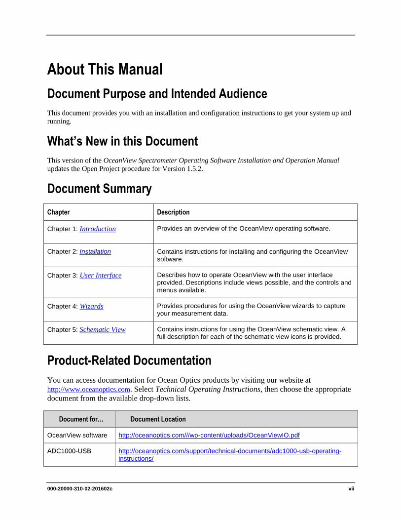
Document Summary
Chapter Description
Chapter 1: Introduction Provides an overview of the OceanView operating software.
Chapter 2: Installation Contains instructions for installing and configuring the OceanView software.
Chapter 3: User Interface Describes how to operate OceanView with the user interface provided. Descriptions include views possible, and the controls and menus available.
Chapter 4: Wizards Provides procedures for using the OceanView wizards to capture your measurement data.
Chapter 5: Schematic View Contains instructions for using the OceanView schematic view. A full description for each of the schematic view icons is provided.
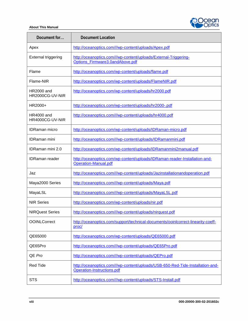
Product-Related Documentation
You can access documentation for Ocean Optics products by visiting our website at
http://www.oceanoptics.com. Select Technical Operating Instructions, then choose the appropriate
document from the available drop-down lists.
Document for… Document Location
OceanView software http://oceanoptics.com///wp-content/uploads/OceanViewIO.pdf
ADC1000-USB http://oceanoptics.com/support/technical-documents/adc1000-usb-operating-instructions/
About This Manual
viii 000-20000-300-02-201602c
Document for… Document Location
Apex http://oceanoptics.com///wp-content/uploads/Apex.pdf
External triggering http://oceanoptics.com///wp-content/uploads/External-Triggering-Options_Firmware3.0andAbove.pdf
Flame http://oceanoptics.com/wp-content/uploads/flame.pdf
Flame-NIR http://oceanoptics.com/wp-content/uploads/FlameNIR.pdf
HR2000 and HR2000CG-UV-NIR
http://oceanoptics.com/wp-content/uploads/hr2000.pdf
HR2000+ http://oceanoptics.com/wp-content/uploads/hr2000-.pdf
HR4000 and HR4000CG-UV-NIR
http://oceanoptics.com///wp-content/uploads/hr4000.pdf
IDRaman micro http://oceanoptics.com/wp-content/uploads/IDRaman-micro.pdf
IDRaman mini http://oceanoptics.com///wp-content/uploads/IDRamanmini.pdf
IDRaman mini 2.0 http://oceanoptics.com/wp-content/uploads/IDRamanmini2manual.pdf
IDRaman reader http://oceanoptics.com/wp-content/uploads/IDRaman-reader-Installation-and-Operation-Manual.pdf
Jaz http://oceanoptics.com///wp-content/uploads/Jazinstallationandoperation.pdf
Maya2000 Series http://oceanoptics.com///wp-content/uploads/Maya.pdf
MayaLSL http://oceanoptics.com///wp-content/uploads/MayaLSL.pdf
NIR Series http://oceanoptics.com/wp-content/uploads/nir.pdf
NIRQuest Series http://oceanoptics.com///wp-content/uploads/nirquest.pdf
OOINLCorrect http://oceanoptics.com/support/technical-documents/ooinlcorrect-linearity-coeff-proc/
QE65000 http://oceanoptics.com/wp-content/uploads/QE65000.pdf
QE65Pro http://oceanoptics.com///wp-content/uploads/QE65Pro.pdf
QE Pro http://oceanoptics.com///wp-content/uploads/QEPro.pdf
Red Tide http://oceanoptics.com///wp-content/uploads/USB-650-Red-Tide-Installation-and-Operation-Instructions.pdf
STS http://oceanoptics.com///wp-content/uploads/STS-Install.pdf
About This Manual
000-20000-310-02-201602c ix
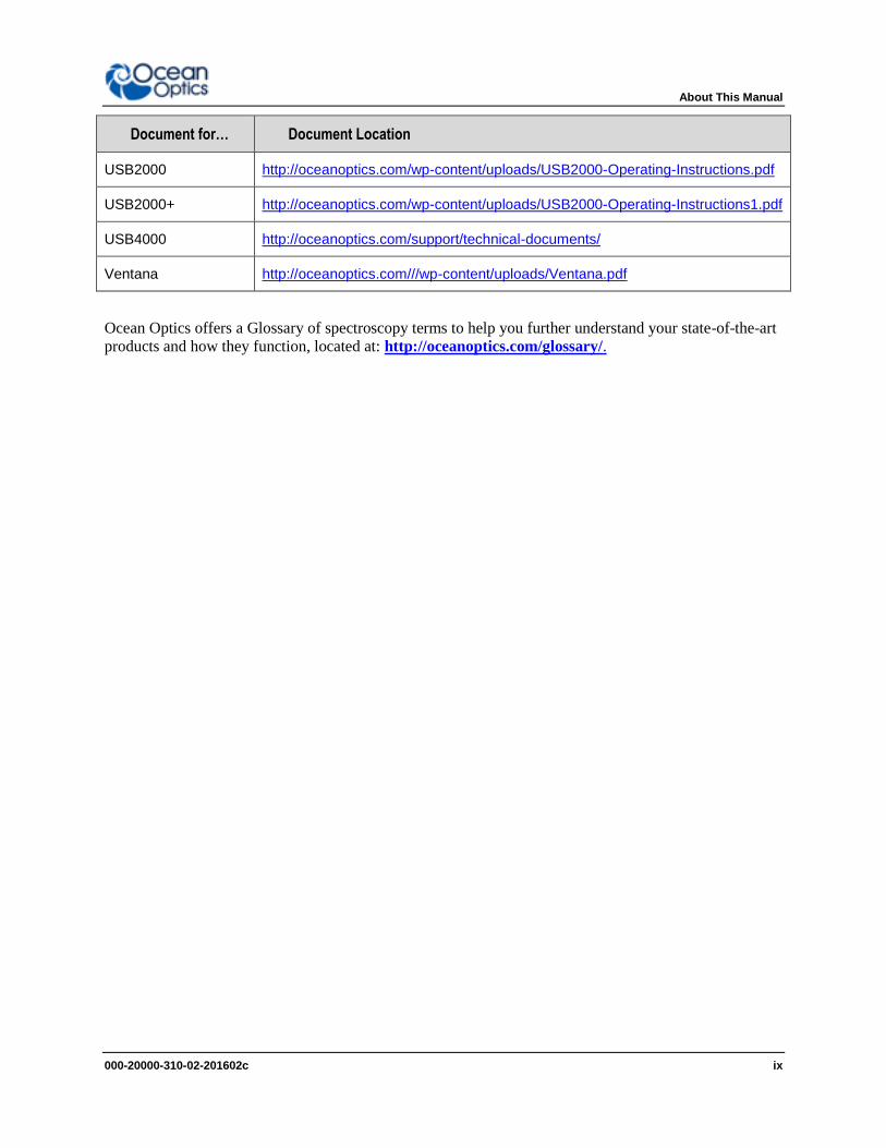
Document for… Document Location
USB2000 http://oceanoptics.com/wp-content/uploads/USB2000-Operating-Instructions.pdf
USB2000+ http://oceanoptics.com/wp-content/uploads/USB2000-Operating-Instructions1.pdf
USB4000 http://oceanoptics.com/support/technical-documents/
Ventana http://oceanoptics.com///wp-content/uploads/Ventana.pdf
Ocean Optics offers a Glossary of spectroscopy terms to help you further understand your state-of-the-art
products and how they function, located at: http://oceanoptics.com/glossary/.

About This Manual
x 000-20000-300-02-201602c
000-20000-310-02-201602c 1
Chapter 1
Introduction
Product Overview Ocean Optics has taken Java-based spectroscopy software to the next level with OceanView. This next
logical step in the evolution of spectrometer software provides good stability, persistence of user settings,
a broad scope of device features, and consistent file saving and loading procedures.
OceanView operates on 32- and 64-bit Windows, Macintosh and Linux operating systems. The software
can control any Ocean Optics USB spectrometer.
For the latest release notes, see OceanView on our Software Downloads page.
USB Spectrometer and Device Control OceanView easily manages multiple USB communication spectrometers – each with different acquisition
parameters – in multiple windows, and provides graphical and numeric representation of spectra from
each spectrometer. Using OceanView, you can combine data from multiple sources for applications that
include upwelling/downwelling measurements, dual-beam referencing and process monitoring.
OceanView can be used with the following Ocean Optics spectrometers when they are interfacing to a
computer through their USB port:
Apex 785 Raman Spectrometer
Flame -S and Flame-T Spectrometers
HR2000 High-resolution Spectrometer
HR2000+High-resolution Spectrometer
HR4000 High-resolution Spectrometer
Jaz System
Maya 2000 and Maya2000-Pro Spectrometers
Maya LSL Spectrometer
NIR-512 Near-IR Spectrometer
NIR256-2.1 and NIR256-2.5 Near-IR Spectrometers
NIRQuest512-1.7, NIRQuest512-1.9, 512-2.2 and 512-2.5 Near-IR Spectrometers
NIRQuest256-2.1 and 256-2.5 Near-IR Spectrometers
1: Introduction
2 000-20000-300-02-201602c
QE65000 Scientific-grade Spectrometer
QE65 Pro Scientific-grade Spectrometer
QE Pro Spectrometer
STS Micro Spectrometers
Torus Spectrometer
USB650 Spectrometer
USB2000 Spectrometer
USB2000+ Spectrometer
USB2000-FLG Spectrometer
USB4000 Spectrometer
Ventana High Sensitivity Spectrometers
OceanView also supports the following USB devices:
ADC1000-USB A/D Converter
Flame Direct Attach UV-VIS Integrated Sampling System
Flame Direct Attach VIS-NIR Integrated Sampling System
IDRaman micro
IDRaman mini
IDRaman mini 2.0
IDRaman reader
ISS-UV-VIS
USB-AOUT Analog Output Module
Features Customizable user-interface that allows you to choose what data you want to display and which
items to display on the toolbars and menus.
Persistence of user settings including:
- File locations
- Acquisition parameters
- Menu settings (hiding/showing of menu items)
- Graph view customization
Capability of manually saving project settings (source, processing type, acquisition parameters, data
view customization) and reloading them again later.
Ability to perform specialized calculations on spectral and other measurement data, including:
- Derivatives and integrals of spectral data
2: Introduction
000-20000-310-02-201602c 3
- Spectral arithmetic
- Ratiometric on the same spectrum or between 2 different spectra
- Interpolation, subsetting and concatenation of a spectrum
Support of the following experiments/processing modes:
- Quick View (formerly Scope Mode)
- Quick View Minus Background
- Absorbance
- Reflection
- Fluorescence
- Transmission
- Raman
- Quick View Fluorescence
- Relative Irradiance
- Absolute Irradiance
- Color
- Photometry
- Concentration
- Energy, Power, Photons
- Strip Charts
- Spectral Math/Arithmetic
- Spectral Splicing
- Color
- Photometry
- Peak metrics
Schematic view for processing spectral data on the fly and for customizing your experiment (data
acquisition)
1: Introduction
4 000-20000-300-02-201602c
Spectroscopic Functions OceanView allows you to perform the three basic spectroscopic experiments – absorbance, reflectance
and emission, as well as absolute irradiance and Raman. Signal-processing functions such as electrical
dark-signal correction, boxcar pixel smoothing and signal averaging are also included. Scope mode, the
spectrometer operating mode in which raw data (signal) is acquired by the detector, allows you to
establish these signal-conditioning parameters. The basic concept for the software is that real-time display
of data allows users to evaluate the effectiveness of their experimental setups and data processing
selections, make changes to these parameters, instantly see the effects and save the data. Most
spectrometer-system operating software does not allow such signal-conditioning flexibility.
With OceanView, you can perform time-acquisition experiments for kinetics applications. As part of the
time-acquisition function (strip charts), you can monitor and report single wavelengths, and you can
average between wavelengths and find the integral between two wavelengths. In addition, you can
perform reference monitoring in a variety of ways: single wavelength (1 or 2 channels), integrated
intensity (starting and ending wavelengths for 1 or 2 channels) and wavelength-by-wavelength (2
channels).
OceanView gives you complete control of setting the parameters for all system functions such as
acquiring data, designing the graph display, and using spectra overlays. OceanView has the benefit of
providing various software-controlled triggering options for external events such as laser firing or light
source pulsing.
Other advanced features give you several data-collection options. You can independently store and
retrieve dark, reference, sample and processed spectra. All data can be saved to disk using
autoincremented filenames. You can save data as ASCII files. One feature prints the spectra and another
copies spectral data into other software such as Excel and Word.
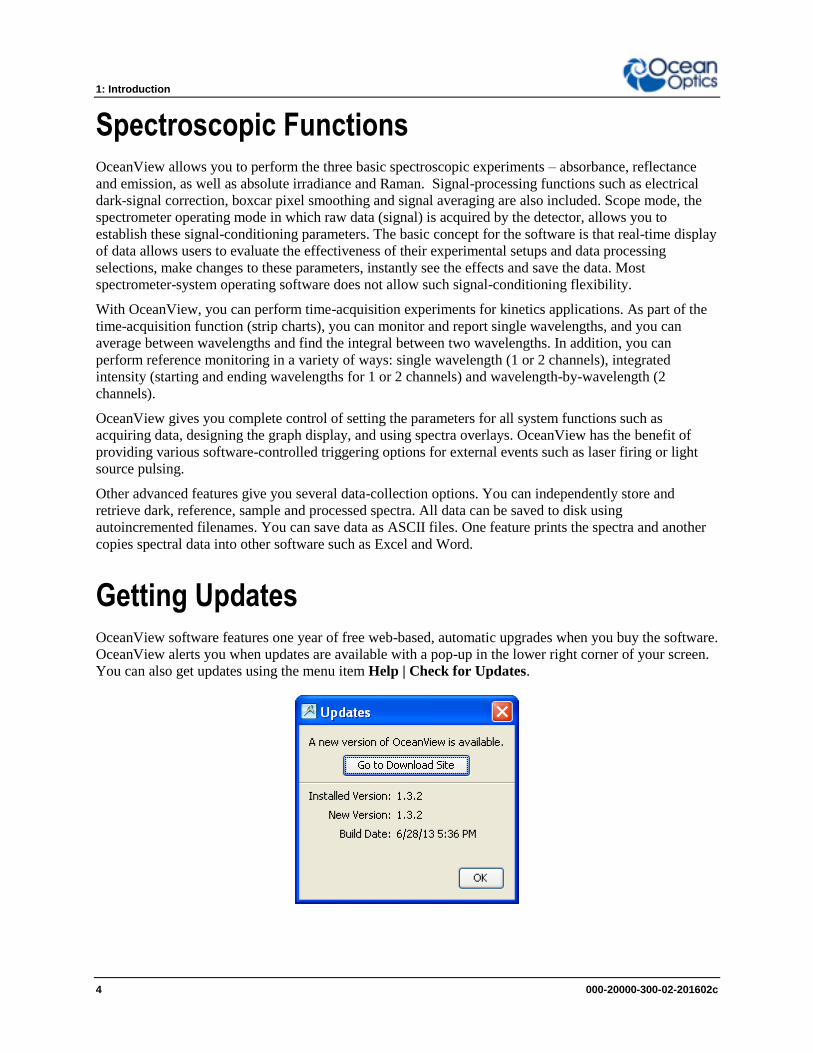
Getting Updates OceanView software features one year of free web-based, automatic upgrades when you buy the software.
OceanView alerts you when updates are available with a pop-up in the lower right corner of your screen.
You can also get updates using the menu item Help | Check for Updates.
000-20000-310-02-201602c 5
Chapter 2
Installation
Overview The following sections will guide you in installing OceanView on a Windows, Macintosh or Linux
operating system.
Caution Do NOT connect the spectrometer to the computer until you install the OceanView
software. Follow the instructions below to properly connect and configure your
system.
OceanView Minimum System Requirements Monitor resolution: 1024 X 768 or higher
RAM: 1.5 GB or higher
Processor: Intel Core II Duo @ 1.4 GHz or better
Intel Core Duo @ 2.0 GHz or better
AMD Athlon Neo X2 @ 1.6 GHz or better
Intel Atom @ 2.13 GHz or better
AMD Athlon 64 x2 @ 1.7 GHz or better
HD Space: 300 MB free space
Note
Most processors produced in 2010 and later should work well with OceanView. OceanView does
not run on tablets with ARM processors.
Installation Download OceanView from the link you received in your e-mail. If you have purchased a CD, download
the file appropriate for your computer system from the CD.
Installation instructions are included below for installing OceanView on each of the following operating
systems:
Microsoft Windows – XP, Vista, 7, 8, 8.1, 10; 32-bit and 64-bit

2: Installation
6 000-20000-300-02-201602c
Note
Do not install OceanView on a Windows 32-bit computer that is currently running SpectraSuite
or OmniDriver (and using EZUSB).
Apple Macintosh – OSX 10.5 or higher on Intel processor
Linux – Any version released for an x86 or amd64 platform since 2010
Example: CentOS(Version 5.5), and Ubuntu (version 10.4LTS)
Installing on a Windows Platform
Total download is approximately 64 MB (32-bit) or 71 MB (64-bit).
► Procedure
1. Close all other applications running on the computer.
2. Start Internet Explorer.
3. Navigate to the link you received to the OceanView software in your email and click on
the OceanView software appropriate for your Windows operating system.
4. Save the software to the desired location. The default installation directory is \Program
Files\Ocean Optics\OceanView.
5. The installer wizard guides you through the installation process. The OceanView icon
location is Start | Programs | Ocean Optics | OceanView | OceanView and the current
user’s desktop.
Device Driver Issues
Hardware device driver installation is seamless on Microsoft Windows operating systems when you
connect your spectrometer to your computer. However, some Windows systems can require a bit more
care when connecting your spectrometer for the first time.
If your spectrometer is not recognized by OceanView running on your computer, you need to manually
install the spectrometer drivers using the procedure below.
Windows Driver Manual Installation Process
Use the following procedure when connecting your spectrometer to a Windows system. Steps may vary
slightly depending on the version of Windows.
► Procedure
1. Open the Control Panel and click Device Manager.
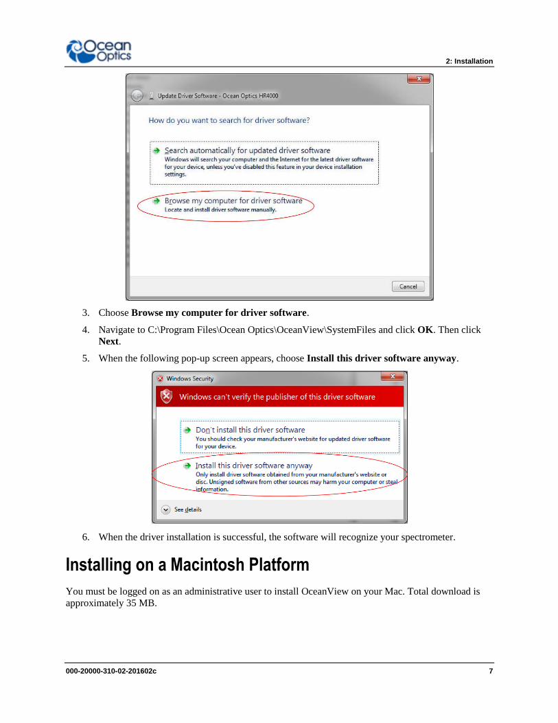
2. Under Other devices, right-click on the Ocean Optics spectrometer and choose update driver
software. The following screen appears:
2: Installation
000-20000-310-02-201602c 7
3. Choose Browse my computer for driver software.
4. Navigate to C:\Program Files\Ocean Optics\OceanView\SystemFiles and click OK. Then click
Next.
5. When the following pop-up screen appears, choose Install this driver software anyway.
6. When the driver installation is successful, the software will recognize your spectrometer.
Installing on a Macintosh Platform
You must be logged on as an administrative user to install OceanView on your Mac. Total download is
approximately 35 MB.
2: Installation
8 000-20000-300-02-201602c
Note
Newer versions of MacOSX do not ship with Java so you may need to manually install a recent
Java release before installing OceanView. Instructions to download a recent Java release for
different versions of OSX can be found at: http://support.apple.com/kb/HT5648
There is also a direct link for the Java for OSX 10.7.3 and newer at:
http://www.java.com/en/download/manual.jsp#mac
► Procedure
1. Navigate to the link you received to the OceanView software and download the installer
(OceanViewSetup_Mac.dmg).
2. Double-click the OceanViewSetup_Mac.dmg file to mount the disk image. A new OceanView
icon resembling a disk drive appears on your desktop. The new icon should open automatically (if
it doesn’t, double-click it).
3. Drag the OceanView.app icon to the Applications folder icon to install. OceanView can then be
launched from the Applications folder. If desired, double-click the Applications folder and drag
the OceanView icon from Applications to the Dock to be able to launch it more conveniently.
4. When the installation is complete, drag the OceanView drive icon to the trash can.
Installing on a Linux Platform
Total download is approximately 75 MB (32-bit) or 67 MB (64-bit).
► Procedure
1. Navigate to the link you received to the OceanView software in your email and download the
appropriate Linux OceanView installer.
Note
The example below is for a 64 bit installer downloaded to the desktop. Change 64 to 32 and the
file location as needed for your installation.
2. Start a terminal window and enter the following commands:
chmod 755 ~/Desktop/OceanViewSetup_Linux64.bin
gksudo ~/Desktop/OceanViewSetup_Linux64.bin
You are prompted for your password, which allows you to execute the setup as root. Contact your
system administrator if you do not have the password. If the gksudo command does not work (it
may not be set up for your user account), then enter the following:
su
(enter password for root)
~/Desktop/OceanViewSetup_Linux64.bin
2: Installation
000-20000-310-02-201602c 9
The Linux version of OceanView requires some libraries that may not be installed by default,
depending on the Linux distribution. The following are libraries are required and are not provided
as part of OceanView:
- libstdc++ version 6 or newer
- libXp version 6 or newer
- libusb version 0.1.10 or newer (should be provided in a libusb package or can be
downloaded from http://libusb.sourceforge.net/download.html#stable)
3. It may be necessary to modify SELinux (Security Enhanced Linux) restrictions before
OceanView will run. It is possible to remove SELinux auditing by running 'setenforce Permissive'
as root or by customizing your SELinux policies. The OceanView installer does not modify
system security settings.
Note
The default installation directory is /usr/local/OceanOptics/OceanView.
A symbolic link is put in /usr/bin so that you can enter OceanView on any command line to start
the program.
The OceanView icon location varies by installation, but will be under either Applications or
Other under the Application Launcher menu.
Retrieving from a CD
If you purchased a CD for OceanView, use this procedure to retrieve the installation files.
► Procedure
1. Insert the CD that you received containing your OceanView software into your computer.
2. Select the OceanView software for your computer’s operating platform via the CD interface.
Then follow the prompts in the installation wizard.
--OR--
Browse to the appropriate OceanView set-up file for your computer and double-click it to start the
software installation. Set-up files are as follows:
Windows 32-bit: OceanViewSetup_Windows32.exe
Windows 64-bit: OceanViewSetup_Windows64.exe
Mac: OceanViewSetup_Mac.dmg
Linux 32-bit: OceanViewSetup_Linux32.bin
Linux 64-bit: OceanViewSetup_Linux64.bin
2: Installation
10 000-20000-300-02-201602c
Product Activation
Licensing
You can activate your OceanView software conveniently online by selecting Help --> Licensing and
entering the product key in the OceanView Licensing dialog box that you received when you purchased
the software when you first install the software.
If you do not have an Internet connection, click Offline Registration to display the Product Activation
wizard. Using this wizard, you can then save an activation request file and send it to Ocean Optics via an
Internet-connected device. Ocean Optics will then reply with your Activation Request file that you must
apply using Step 3 of the Product Activation wizard.
The OceanView Licensing dialog box also allows you to deactivate your software license.
Starting Your 10 Day Free Trial
If you have downloaded OceanView with the 10-day free trial, you will have access to full functionality
when you activate your license. All data and projects saved during your 10 day free trial will be available
when the software is activated using a valid product key. Contact [email protected] to purchase
OceanView licenses.
► Procedure
1. Double-click the OceanView icon on your Desktop to start the software.
2. Click the Cancel button in the OceanView Product Activation dialog box that opens to start your
10 day free trial with a fully functional version of OceanView.
Using Your Product Key to Activate Your Software
Note
An Internet connection is required to activate your software using a valid product key. If an
Internet connection is not available, contact [email protected] for the offline activation
procedure.
► Procedure
1. Double-click the OceanView icon ( ) on your Desktop to start the software.
2. Click Next in the OceanView Product Activation dialog box to enter your product key.
3. Copy the product key from the email you received and paste it into the product key box.
4. Click the Register Software button to validate your product key.
5. Click Finish to complete the software registration.

2: Installation
000-20000-310-02-201602c 11
If you see the message below, check your Internet connection and click the Register Software button
again. If the computer is connected to the Internet and you still cannot register your software, contact
[email protected] for assistance.
Deactivating Your Product Key for Software Installation on Another Computer With the exception of multi-license packs, your product key is only valid for use on two computers at a
time. A deactivation option is available in OceanView if you want to deactivate your product key on one
computer so you can use it on another computer.
► Procedure
1. Go to Help | Licensing.
2. Click Deactivate. The following warning will appear:
3. Click Yes to deactivate the license. OceanView closes and the license will be available for use on
another computer.
Connecting Your Spectrometer Once you have installed OceanView, you can install your spectrometer. Most Ocean Optics spectrometers
connect to your computer using a USB cable. However, refer to your spectrometer manual for specific
spectrometer installation instructions (see Product-Related Documentation). Be sure to allow sufficient
time for the drivers to install before starting OceanView.

2: Installation
12 000-20000-300-02-201602c
000-20000-310-02-201602c 13
Chapter 3
User Interface
Launching OceanView Once you have installed your software and connected your spectrometer, you are ready start using
OceanView. Launching OceanView differs, depending on your operating system and where you have
placed your OceanView program files.
For PCs running Microsoft Windows, the default location is Start | Programs | Ocean Optics |
OceanView | OceanView.
For Mac computers, the default location is the Applications folder.
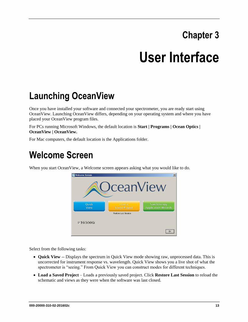
Welcome Screen When you start OceanView, a Welcome screen appears asking what you would like to do.
Select from the following tasks:
Quick View -- Displays the spectrum in Quick View mode showing raw, unprocessed data. This is
uncorrected for instrument response vs. wavelength. Quick View shows you a live shot of what the
spectrometer is “seeing.” From Quick View you can construct modes for different techniques.
Load a Saved Project – Loads a previously saved project. Click Restore Last Session to reload the
schematic and views as they were when the software was last closed.
3: User interface
14 000-20000-300-02-201602c
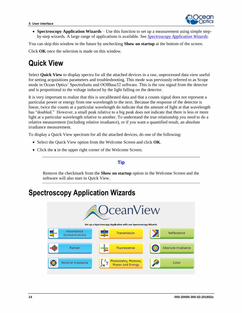
Spectroscopy Application Wizards – Use this function to set up a measurement using simple step-
by-step wizards. A large range of applications is available. See Spectroscopy Application Wizards.
You can skip this window in the future by unchecking Show on startup at the bottom of the screen.
Click OK once the selection is made on this window.
Quick View
Select Quick View to display spectra for all the attached devices in a raw, unprocessed data view useful
for setting acquisitions parameters and troubleshooting. This mode was previously referred to as Scope
mode in Ocean Optics’ SpectraSuite and OOIBase32 software. This is the raw signal from the detector
and is proportional to the voltage induced by the light falling on the detector.
It is very important to realize that this is uncalibrated data and that a counts signal does not represent a
particular power or energy from one wavelength to the next. Because the response of the detector is
linear, twice the counts at a particular wavelength do indicate that the amount of light at that wavelength
has “doubled.” However, a small peak relative to a big peak does not indicate that there is less or more
light at a particular wavelength relative to another. To understand the true relationship you need to do a
relative measurement (including relative irradiance), or if you want a quantified result, an absolute
irradiance measurement.
To display a Quick View spectrum for all the attached devices, do one of the following:
Select the Quick View option from the Welcome Screen and click OK.
Click the x in the upper right corner of the Welcome Screen.
Tip
Remove the checkmark from the Show on startup option in the Welcome Screen and the
software will also start in Quick View.
Spectroscopy Application Wizards
3: User Interface
000-20000-310-02-201602c 15
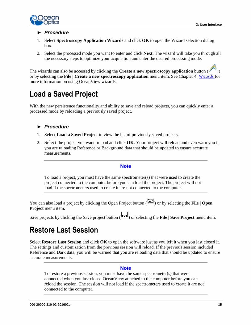
► Procedure
1. Select Spectroscopy Application Wizards and click OK to open the Wizard selection dialog
box.
2. Select the processed mode you want to enter and click Next. The wizard will take you through all
the necessary steps to optimize your acquisition and enter the desired processing mode.
The wizards can also be accessed by clicking the Create a new spectroscopy application button ( )
or by selecting the File | Create a new spectroscopy application menu item. See Chapter 4: Wizards for
more information on using OceanView wizards.
Load a Saved Project
With the new persistence functionality and ability to save and reload projects, you can quickly enter a
processed mode by reloading a previously saved project.
► Procedure
1. Select Load a Saved Project to view the list of previously saved projects.
2. Select the project you want to load and click OK. Your project will reload and even warn you if
you are reloading Reference or Background data that should be updated to ensure accurate
measurements.
Note
To load a project, you must have the same spectrometer(s) that were used to create the
project connected to the computer before you can load the project. The project will not
load if the spectrometers used to create it are not connected to the computer.
You can also load a project by clicking the Open Project button ( ) or by selecting the File | Open
Project menu item.
Save projects by clicking the Save project button ( ) or selecting the File | Save Project menu item.
Restore Last Session
Select Restore Last Session and click OK to open the software just as you left it when you last closed it.
The settings and customization from the previous session will reload. If the previous session included
Reference and Dark data, you will be warned that you are reloading data that should be updated to ensure
accurate measurements.
Note To restore a previous session, you must have the same spectrometer(s) that were
connected when you last closed OceanView attached to the computer before you can
reload the session. The session will not load if the spectrometers used to create it are not
connected to the computer.
3: User interface
16 000-20000-300-02-201602c
Views OceanView offers two different views: Graph View and Schematic View.
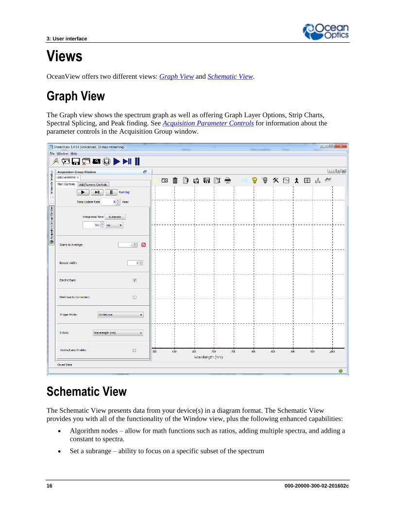
Graph View
The Graph view shows the spectrum graph as well as offering Graph Layer Options, Strip Charts,
Spectral Splicing, and Peak finding. See Acquisition Parameter Controls for information about the
parameter controls in the Acquisition Group window.
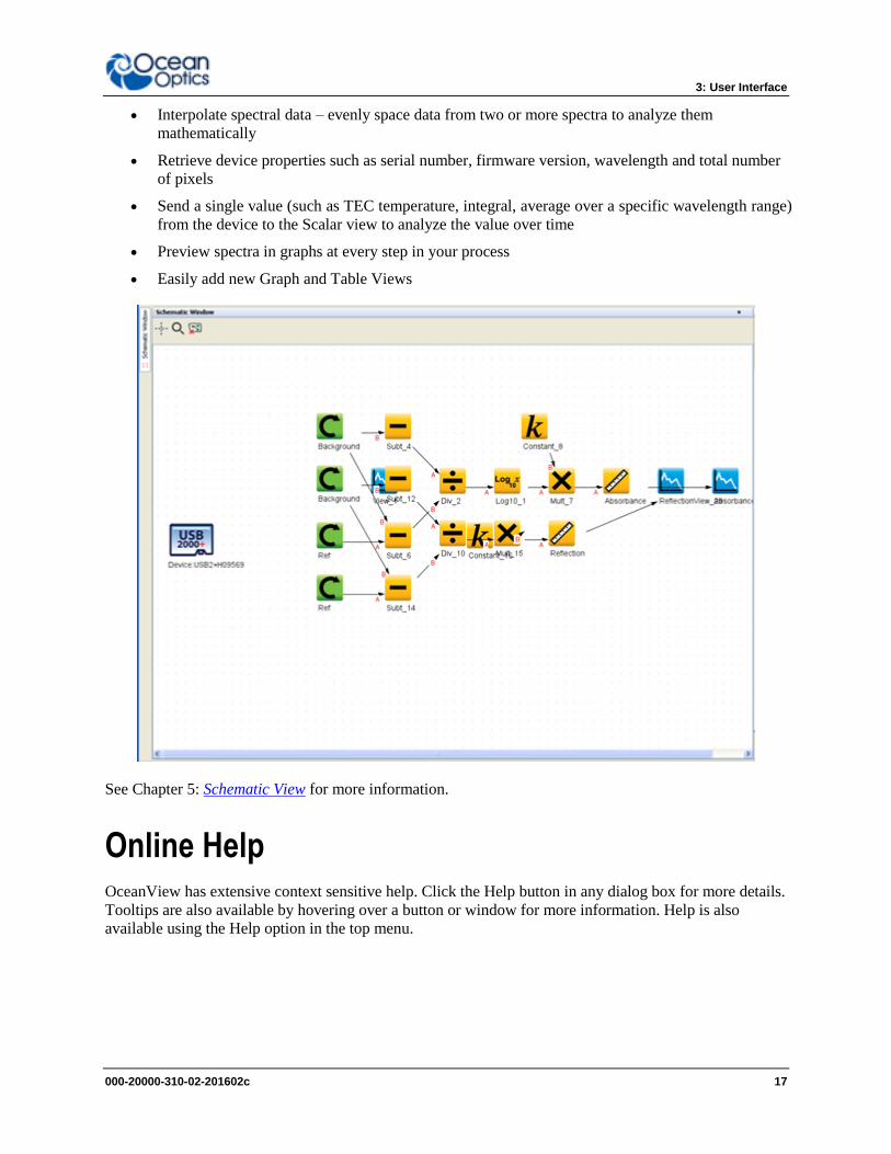
Schematic View
The Schematic View presents data from your device(s) in a diagram format. The Schematic View
provides you with all of the functionality of the Window view, plus the following enhanced capabilities:
Algorithm nodes – allow for math functions such as ratios, adding multiple spectra, and adding a
constant to spectra.
Set a subrange – ability to focus on a specific subset of the spectrum
3: User Interface
000-20000-310-02-201602c 17
Interpolate spectral data – evenly space data from two or more spectra to analyze them
mathematically
Retrieve device properties such as serial number, firmware version, wavelength and total number
of pixels
Send a single value (such as TEC temperature, integral, average over a specific wavelength range)
from the device to the Scalar view to analyze the value over time
Preview spectra in graphs at every step in your process
Easily add new Graph and Table Views
See Chapter 5: Schematic View for more information.
Online Help OceanView has extensive context sensitive help. Click the Help button in any dialog box for more details.
Tooltips are also available by hovering over a button or window for more information. Help is also
available using the Help option in the top menu.
3: User interface
18 000-20000-300-02-201602c
Main Window Controls
Note
Different types of acquisitions are available for different devices including Spectrometer, I²C,
SPI, Board Temperature, Thermo-Electric Cooling and Analog In. The controls available in the
Acquisition Parameters Controls vary based on the type of acquisition is selected.
The Main Window controls at the top of the OceanView screen allow you to perform the following tasks:
Creating a New Spectroscopy Application
Opening a Project
Saving a Project
Removing a Project
Using the Device Manager
Creating a New Spectroscopy Application
Click to choose the application to build. This function is also available from the File Menu.
Absorbance
Raman
Relative Irradiance
Transmission
Fluorescence
Photometry, Photons, Power and Energy
Reflectance
Absolute Irradiance
Color
Opening a Project
Click to navigate to and open a previously stored project. You can also type the shortcut Ctrl + O.
This function is also available from the File Menu.
Saving a Project
Click to save a project in a location that you specify. A single ACII file of that acquisition is saved to
the folder specified; this folder then persists as the default save location every time you use OceanView.
3: User Interface
000-20000-310-02-201602c 19
The icon turns red while the save is in progress. When saving a continuous series of acquisitions, all
spectra are saved starting when you first click this icon until you click it again. Configre the save options
using (see Configure Graph Saving).
Removing a Project
Click to delete a previously stored project. You can also type the shortcut Ctrl + X. This function is
also available from the File Menu.
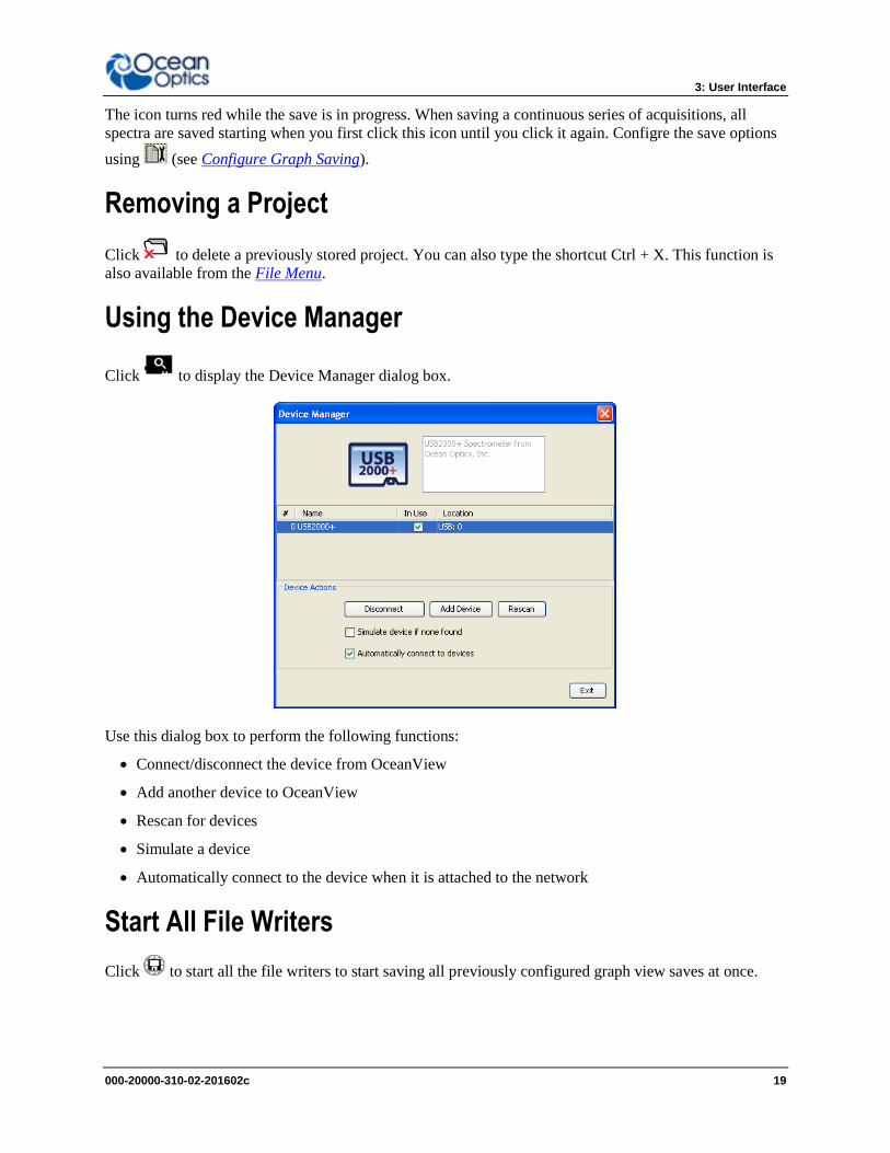
Using the Device Manager
Click to display the Device Manager dialog box.
Use this dialog box to perform the following functions:
Connect/disconnect the device from OceanView
Add another device to OceanView
Rescan for devices
Simulate a device
Automatically connect to the device when it is attached to the network
Start All File Writers
Click to start all the file writers to start saving all previously configured graph view saves at once.
3: User interface
20 000-20000-300-02-201602c
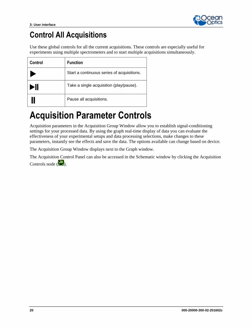
Control All Acquisitions
Use these global controls for all the current acquisitions. These controls are especially useful for
experiments using multiple spectrometers and to start multiple acquisitions simultaneously.
Control Function
Start a continuous series of acquisitions.
Take a single acquisition (play/pause).
Pause all acquisitions.
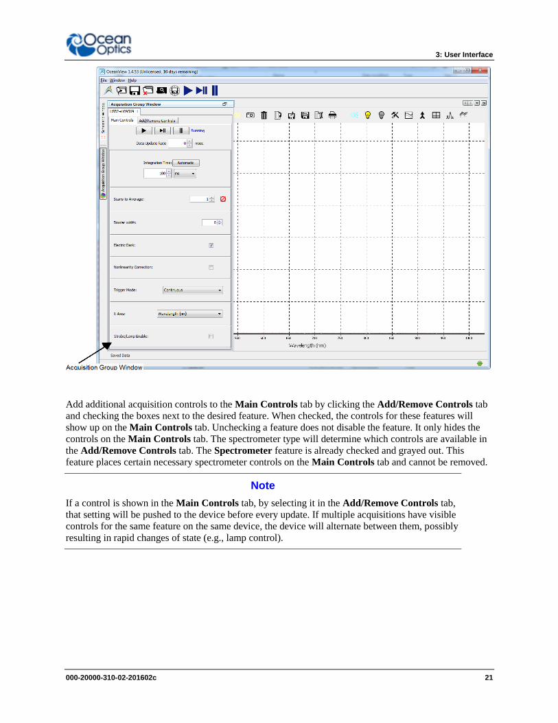
Acquisition Parameter Controls Acquisition parameters in the Acquisition Group Window allow you to establish signal-conditioning
settings for your processed data. By using the graph real-time display of data you can evaluate the
effectiveness of your experimental setups and data processing selections, make changes to these
parameters, instantly see the effects and save the data. The options available can change based on device.
The Acquisition Group Window displays next to the Graph window.
The Acquisition Control Panel can also be accessed in the Schematic window by clicking the Acquisition
Controls node ( ).
3: User Interface
000-20000-310-02-201602c 21
Add additional acquisition controls to the Main Controls tab by clicking the Add/Remove Controls tab
and checking the boxes next to the desired feature. When checked, the controls for these features will
show up on the Main Controls tab. Unchecking a feature does not disable the feature. It only hides the
controls on the Main Controls tab. The spectrometer type will determine which controls are available in
the Add/Remove Controls tab. The Spectrometer feature is already checked and grayed out. This
feature places certain necessary spectrometer controls on the Main Controls tab and cannot be removed.
Note
If a control is shown in the Main Controls tab, by selecting it in the Add/Remove Controls tab,
that setting will be pushed to the device before every update. If multiple acquisitions have visible
controls for the same feature on the same device, the device will alternate between them, possibly
resulting in rapid changes of state (e.g., lamp control).
3: User interface
22 000-20000-300-02-201602c
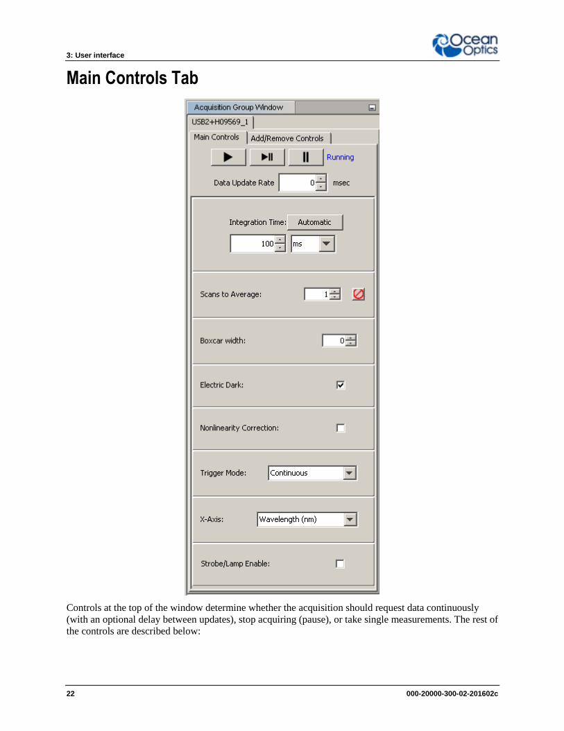
Main Controls Tab
Controls at the top of the window determine whether the acquisition should request data continuously
(with an optional delay between updates), stop acquiring (pause), or take single measurements. The rest of
the controls are described below:
3: User Interface
000-20000-310-02-201602c 23
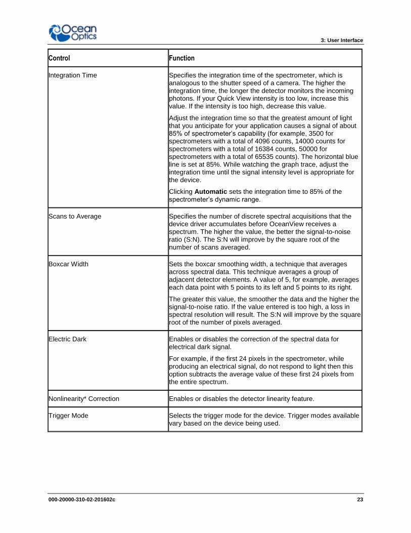
Control Function
Integration Time
Specifies the integration time of the spectrometer, which is analogous to the shutter speed of a camera. The higher the integration time, the longer the detector monitors the incoming photons. If your Quick View intensity is too low, increase this value. If the intensity is too high, decrease this value.
Adjust the integration time so that the greatest amount of light that you anticipate for your application causes a signal of about 85% of spectrometer’s capability (for example, 3500 for spectrometers with a total of 4096 counts, 14000 counts for spectrometers with a total of 16384 counts, 50000 for spectrometers with a total of 65535 counts). The horizontal blue line is set at 85%. While watching the graph trace, adjust the integration time until the signal intensity level is appropriate for the device.
Clicking Automatic sets the integration time to 85% of the spectrometer’s dynamic range.
Scans to Average Specifies the number of discrete spectral acquisitions that the device driver accumulates before OceanView receives a spectrum. The higher the value, the better the signal-to-noise ratio (S:N). The S:N will improve by the square root of the number of scans averaged.
Boxcar Width Sets the boxcar smoothing width, a technique that averages across spectral data. This technique averages a group of adjacent detector elements. A value of 5, for example, averages each data point with 5 points to its left and 5 points to its right.
The greater this value, the smoother the data and the higher the signal-to-noise ratio. If the value entered is too high, a loss in spectral resolution will result. The S:N will improve by the square root of the number of pixels averaged.
Electric Dark Enables or disables the correction of the spectral data for electrical dark signal.
For example, if the first 24 pixels in the spectrometer, while producing an electrical signal, do not respond to light then this option subtracts the average value of these first 24 pixels from the entire spectrum.
Nonlinearity* Correction Enables or disables the detector linearity feature.
Trigger Mode Selects the trigger mode for the device. Trigger modes available vary based on the device being used.
3: User interface
24 000-20000-300-02-201602c
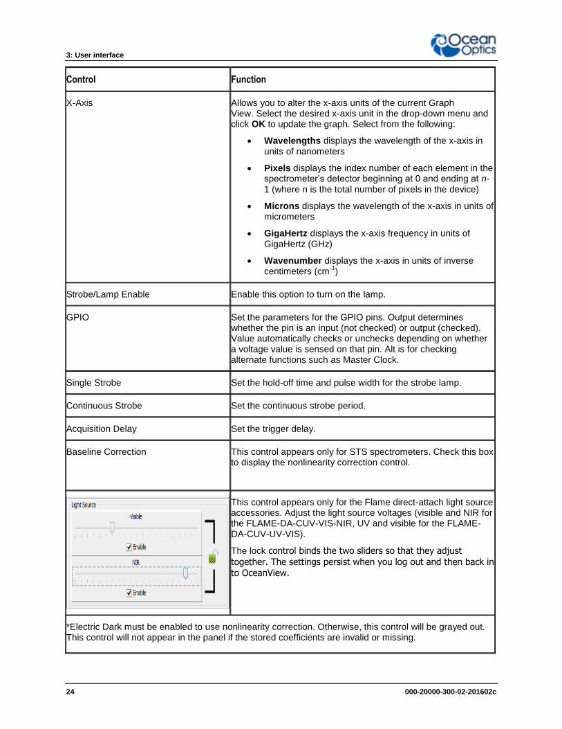
Control Function
X-Axis Allows you to alter the x-axis units of the current Graph View. Select the desired x-axis unit in the drop-down menu and click OK to update the graph. Select from the following:
Wavelengths displays the wavelength of the x-axis in units of nanometers
Pixels displays the index number of each element in the spectrometer’s detector beginning at 0 and ending at n-1 (where n is the total number of pixels in the device)
Microns displays the wavelength of the x-axis in units of micrometers
GigaHertz displays the x-axis frequency in units of GigaHertz (GHz)
Wavenumber displays the x-axis in units of inverse centimeters (cm
-1)
Strobe/Lamp Enable Enable this option to turn on the lamp.
GPIO Set the parameters for the GPIO pins. Output determines whether the pin is an input (not checked) or output (checked). Value automatically checks or unchecks depending on whether a voltage value is sensed on that pin. Alt is for checking alternate functions such as Master Clock.
Single Strobe Set the hold-off time and pulse width for the strobe lamp.
Continuous Strobe Set the continuous strobe period.
Acquisition Delay Set the trigger delay.
Baseline Correction This control appears only for STS spectrometers. Check this box to display the nonlinearity correction control.
This control appears only for the Flame direct-attach light source accessories. Adjust the light source voltages (visible and NIR for the FLAME-DA-CUV-VIS-NIR, UV and visible for the FLAME-DA-CUV-UV-VIS).
The lock control binds the two sliders so that they adjust
together. The settings persist when you log out and then back in to OceanView.
*Electric Dark must be enabled to use nonlinearity correction. Otherwise, this control will be grayed out. This control will not appear in the panel if the stored coefficients are invalid or missing.
3: User Interface
000-20000-310-02-201602c 25
Note
For NIRQuest spectrometers, a dark spectrum must be stored first. A dark spectrum is different
from a background spectrum since a dark spectrum is totally devoid of light. A dark spectrum is
stored by clicking Store Now in the No dark spectrum stored section of the Acquisition
Parameter Controls panel. Once a dark spectrum is stored, nonlinearity can be set.
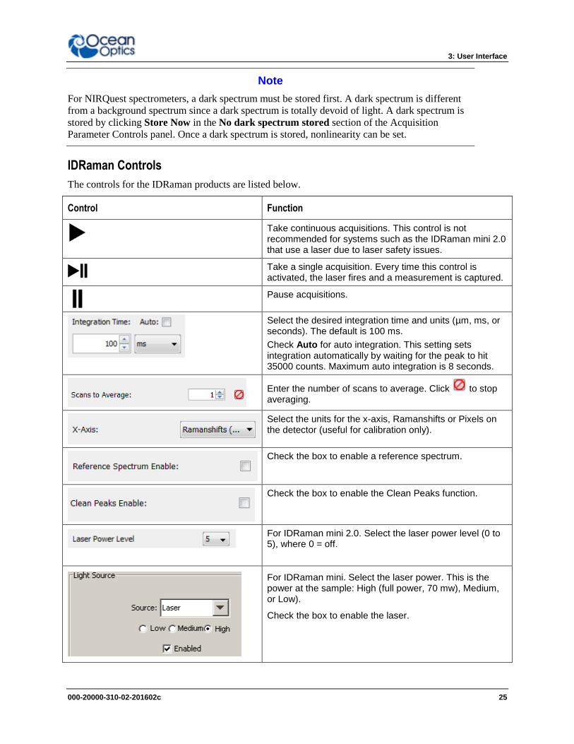
IDRaman Controls
The controls for the IDRaman products are listed below.
Control Function
Take continuous acquisitions. This control is not recommended for systems such as the IDRaman mini 2.0 that use a laser due to laser safety issues.
Take a single acquisition. Every time this control is activated, the laser fires and a measurement is captured.
Pause acquisitions.
Select the desired integration time and units (µm, ms, or seconds). The default is 100 ms.
Check Auto for auto integration. This setting sets integration automatically by waiting for the peak to hit 35000 counts. Maximum auto integration is 8 seconds.
Enter the number of scans to average. Click to stop averaging.
Select the units for the x-axis, Ramanshifts or Pixels on the detector (useful for calibration only).
Check the box to enable a reference spectrum.
Check the box to enable the Clean Peaks function.
For IDRaman mini 2.0. Select the laser power level (0 to 5), where 0 = off.
For IDRaman mini. Select the laser power. This is the power at the sample: High (full power, 70 mw), Medium, or Low).
Check the box to enable the laser.
3: User interface
26 000-20000-300-02-201602c
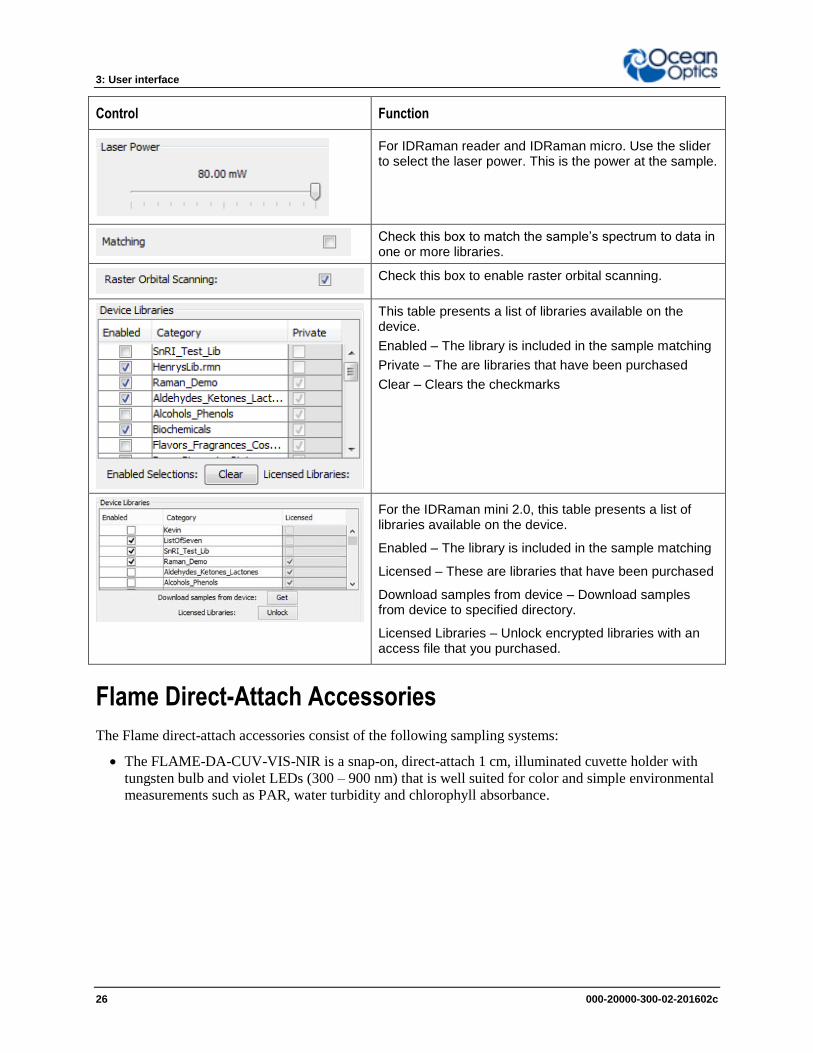
Control Function
For IDRaman reader and IDRaman micro. Use the slider to select the laser power. This is the power at the sample.
Check this box to match the sample’s spectrum to data in one or more libraries.
Check this box to enable raster orbital scanning.
This table presents a list of libraries available on the device.
Enabled – The library is included in the sample matching
Private – The are libraries that have been purchased
Clear – Clears the checkmarks
For the IDRaman mini 2.0, this table presents a list of libraries available on the device.
Enabled – The library is included in the sample matching
Licensed – These are libraries that have been purchased
Download samples from device – Download samples from device to specified directory.
Licensed Libraries – Unlock encrypted libraries with an access file that you purchased.
Flame Direct-Attach Accessories
The Flame direct-attach accessories consist of the following sampling systems:
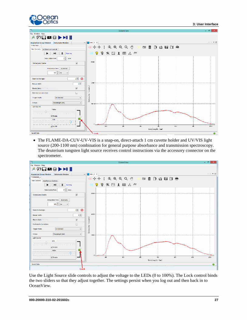
The FLAME-DA-CUV-VIS-NIR is a snap-on, direct-attach 1 cm, illuminated cuvette holder with
tungsten bulb and violet LEDs (300 – 900 nm) that is well suited for color and simple environmental
measurements such as PAR, water turbidity and chlorophyll absorbance.
3: User Interface
000-20000-310-02-201602c 27
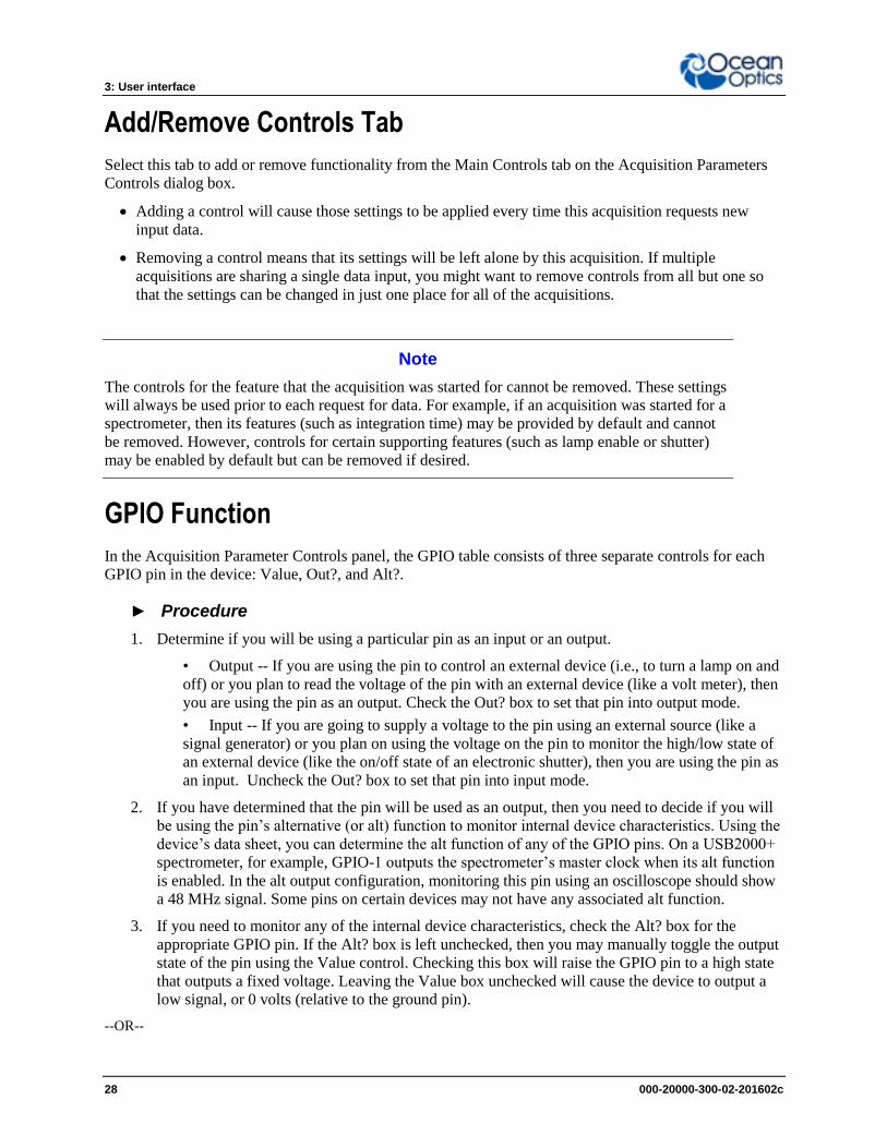
The FLAME-DA-CUV-UV-VIS is a snap-on, direct-attach 1 cm cuvette holder and UV/VIS light
source (200-1100 nm) combination for general purpose absorbance and transmission spectroscopy.
The deuterium tungsten light source receives control instructions via the accessory connector on the
spectrometer.
Use the Light Source slide controls to adjust the voltage to the LEDs (0 to 100%). The Lock control binds
the two sliders so that they adjust together. The settings persist when you log out and then back in to
OceanView.
3: User interface
28 000-20000-300-02-201602c
Add/Remove Controls Tab
Select this tab to add or remove functionality from the Main Controls tab on the Acquisition Parameters
Controls dialog box.
Adding a control will cause those settings to be applied every time this acquisition requests new
input data.
Removing a control means that its settings will be left alone by this acquisition. If multiple
acquisitions are sharing a single data input, you might want to remove controls from all but one so
that the settings can be changed in just one place for all of the acquisitions.
Note
The controls for the feature that the acquisition was started for cannot be removed. These settings
will always be used prior to each request for data. For example, if an acquisition was started for a
spectrometer, then its features (such as integration time) may be provided by default and cannot
be removed. However, controls for certain supporting features (such as lamp enable or shutter)
may be enabled by default but can be removed if desired.
GPIO Function
In the Acquisition Parameter Controls panel, the GPIO table consists of three separate controls for each
GPIO pin in the device: Value, Out?, and Alt?.
► Procedure
1. Determine if you will be using a particular pin as an input or an output.
• Output -- If you are using the pin to control an external device (i.e., to turn a lamp on and
off) or you plan to read the voltage of the pin with an external device (like a volt meter), then
you are using the pin as an output. Check the Out? box to set that pin into output mode.
• Input -- If you are going to supply a voltage to the pin using an external source (like a
signal generator) or you plan on using the voltage on the pin to monitor the high/low state of
an external device (like the on/off state of an electronic shutter), then you are using the pin as
an input. Uncheck the Out? box to set that pin into input mode.
2. If you have determined that the pin will be used as an output, then you need to decide if you will
be using the pin’s alternative (or alt) function to monitor internal device characteristics. Using the
device’s data sheet, you can determine the alt function of any of the GPIO pins. On a USB2000+
spectrometer, for example, GPIO-1 outputs the spectrometer’s master clock when its alt function
is enabled. In the alt output configuration, monitoring this pin using an oscilloscope should show
a 48 MHz signal. Some pins on certain devices may not have any associated alt function.
3. If you need to monitor any of the internal device characteristics, check the Alt? box for the
appropriate GPIO pin. If the Alt? box is left unchecked, then you may manually toggle the output
state of the pin using the Value control. Checking this box will raise the GPIO pin to a high state
that outputs a fixed voltage. Leaving the Value box unchecked will cause the device to output a
low signal, or 0 volts (relative to the ground pin).
--OR--
3: User Interface
000-20000-310-02-201602c 29
4. If the pin is to be used as an input, the Value box will act as an indicator rather than a control. If
the voltage applied to the pin by an external source is above the threshold value, then the Value
box in the GPIO table will register a check mark. If the voltage applied to the pin below the
threshold value, then the Value box will not register a check mark.
Note
In Schematic View in the Output Control (Output Control) node, the GPIO table consists of three
separate rows of controls for each GPIO pin in the device: output value, output enable, and alt
function. There are two columns for each row:
- Latest Value -- contains the control/indicator check box
- Data Input -- allows you to choose how the check box will be controlled.
Before using GPIO in the Output Control (Output Control) node, make sure that the GPIO feature
in the Acquisition Parameter Controls panel has been disabled.
The controls perform the same functions as their counterparts in the Acquisition Parameter
Controls panel. The main difference is that the check box state for any row in the table can be
controlled manually or by a scalar node in the schematic diagram. A positive value from the
scalar node enables the check box, whereas a negative value disables the check box.
To have a node in the software control the state of a check box, wire a scalar-producing node into
the output control node. This can be a static scalar (like a Constant (Const) node) or a dynamic
scalar (like a Running Average (RunAvg) node). Once the scalar node is wired into the Output
Control, use the drop-down menu in the Data Input column to select the appropriate control for
that row in the GPIO table. If the drop-down menu is left blank, the check box will be controlled
manually.
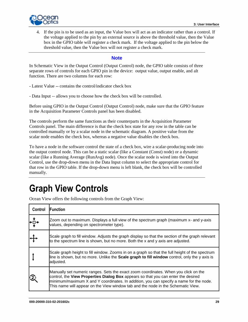
Graph View Controls Ocean View offers the following controls from the Graph View:
Control Function
Zoom out to maximum. Displays a full view of the spectrum graph (maximum x- and y-axis values, depending on spectrometer type).
Scale graph to fill window. Adjusts the graph display so that the section of the graph relevant to the spectrum line is shown, but no more. Both the x and y axis are adjusted.
Scale graph height to fill window. Zooms in on a graph so that the full height of the spectrum line is shown, but no more. Unlike the Scale graph to fill window control, only the y axis is adjusted.
Manually set numeric ranges. Sets the exact zoom coordinates. When you click on the control, the View Properties Dialog Box appears so that you can enter the desired minimum/maximum X and Y coordinates. In addition, you can specify a name for the node. This name will appear on the View window tab and the node in the Schematic View.
3: User interface
30 000-20000-300-02-201602c
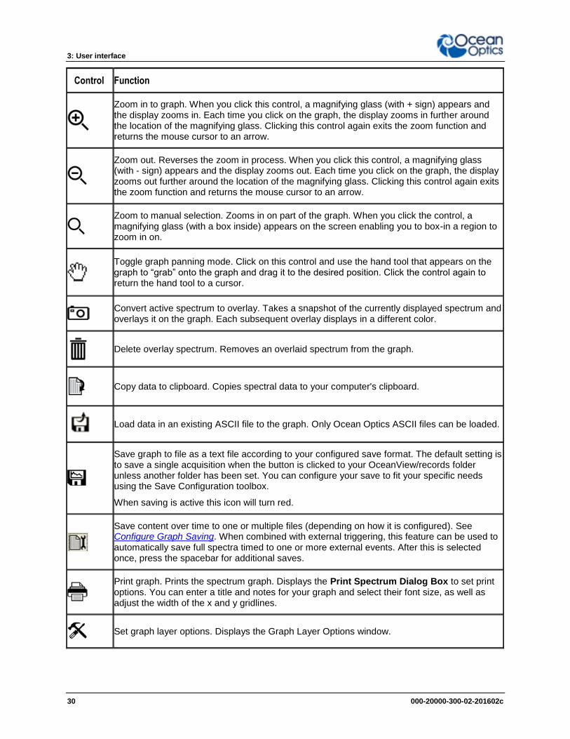
Control Function
Zoom in to graph. When you click this control, a magnifying glass (with + sign) appears and the display zooms in. Each time you click on the graph, the display zooms in further around the location of the magnifying glass. Clicking this control again exits the zoom function and returns the mouse cursor to an arrow.
Zoom out. Reverses the zoom in process. When you click this control, a magnifying glass (with - sign) appears and the display zooms out. Each time you click on the graph, the display zooms out further around the location of the magnifying glass. Clicking this control again exits the zoom function and returns the mouse cursor to an arrow.
Zoom to manual selection. Zooms in on part of the graph. When you click the control, a magnifying glass (with a box inside) appears on the screen enabling you to box-in a region to zoom in on.
Toggle graph panning mode. Click on this control and use the hand tool that appears on the graph to “grab” onto the graph and drag it to the desired position. Click the control again to return the hand tool to a cursor.
Convert active spectrum to overlay. Takes a snapshot of the currently displayed spectrum and overlays it on the graph. Each subsequent overlay displays in a different color.
Delete overlay spectrum. Removes an overlaid spectrum from the graph.
Copy data to clipboard. Copies spectral data to your computer's clipboard.
Load data in an existing ASCII file to the graph. Only Ocean Optics ASCII files can be loaded.
Save graph to file as a text file according to your configured save format. The default setting is to save a single acquisition when the button is clicked to your OceanView/records folder unless another folder has been set. You can configure your save to fit your specific needs using the Save Configuration toolbox.
When saving is active this icon will turn red.
Save content over time to one or multiple files (depending on how it is configured). See Configure Graph Saving. When combined with external triggering, this feature can be used to automatically save full spectra timed to one or more external events. After this is selected once, press the spacebar for additional saves.
Print graph. Prints the spectrum graph. Displays the Print Spectrum Dialog Box to set print options. You can enter a title and notes for your graph and select their font size, as well as adjust the width of the x and y gridlines.
Set graph layer options. Displays the Graph Layer Options window.
3: User Interface
000-20000-310-02-201602c 31
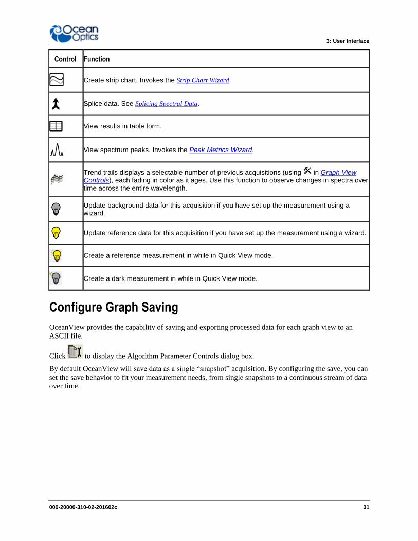
Control Function
Create strip chart. Invokes the Strip Chart Wizard.
Splice data. See Splicing Spectral Data.
View results in table form.
View spectrum peaks. Invokes the Peak Metrics Wizard.
Trend trails displays a selectable number of previous acquisitions (using in Graph View Controls), each fading in color as it ages. Use this function to observe changes in spectra over time across the entire wavelength.
Update background data for this acquisition if you have set up the measurement using a wizard.
Update reference data for this acquisition if you have set up the measurement using a wizard.
Create a reference measurement in while in Quick View mode.
Create a dark measurement in while in Quick View mode.
Configure Graph Saving
OceanView provides the capability of saving and exporting processed data for each graph view to an
ASCII file.
Click to display the Algorithm Parameter Controls dialog box.
By default OceanView will save data as a single “snapshot” acquisition. By configuring the save, you can
set the save behavior to fit your measurement needs, from single snapshots to a continuous stream of data
over time.
3: User interface
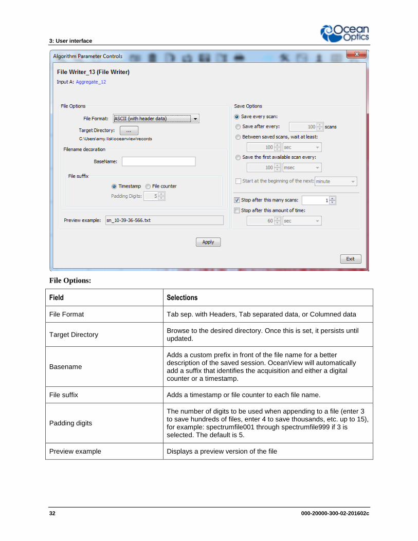
32 000-20000-300-02-201602c
File Options:
Field Selections
File Format Tab sep. with Headers, Tab separated data, or Columned data
Target Directory Browse to the desired directory. Once this is set, it persists until updated.
Basename
Adds a custom prefix in front of the file name for a better description of the saved session. OceanView will automatically add a suffix that identifies the acquisition and either a digital counter or a timestamp.
File suffix Adds a timestamp or file counter to each file name.
Padding digits
The number of digits to be used when appending to a file (enter 3 to save hundreds of files, enter 4 to save thousands, etc. up to 15), for example: spectrumfile001 through spectrumfile999 if 3 is selected. The default is 5.
Preview example Displays a preview version of the file
3: User Interface
000-20000-310-02-201602c 33
Save Options:
Field Selections
Save every scan Saves after every scan
Update after every x scans Saves after the number of scans selected
Between saved scans, wait at least Saves each scan according to the selected the interval
Save the first available scan every The first scan occurs after the interval selected
Start at the beginning of the next Start the scan at the next minute, hour, or day
Stop after this many scans Stops saving after the number of scans selected
Stop after this amount of time Stops saving after the amount of time selected.
Once the saving of graph data has been configured, you can save the graph data to a file or files.
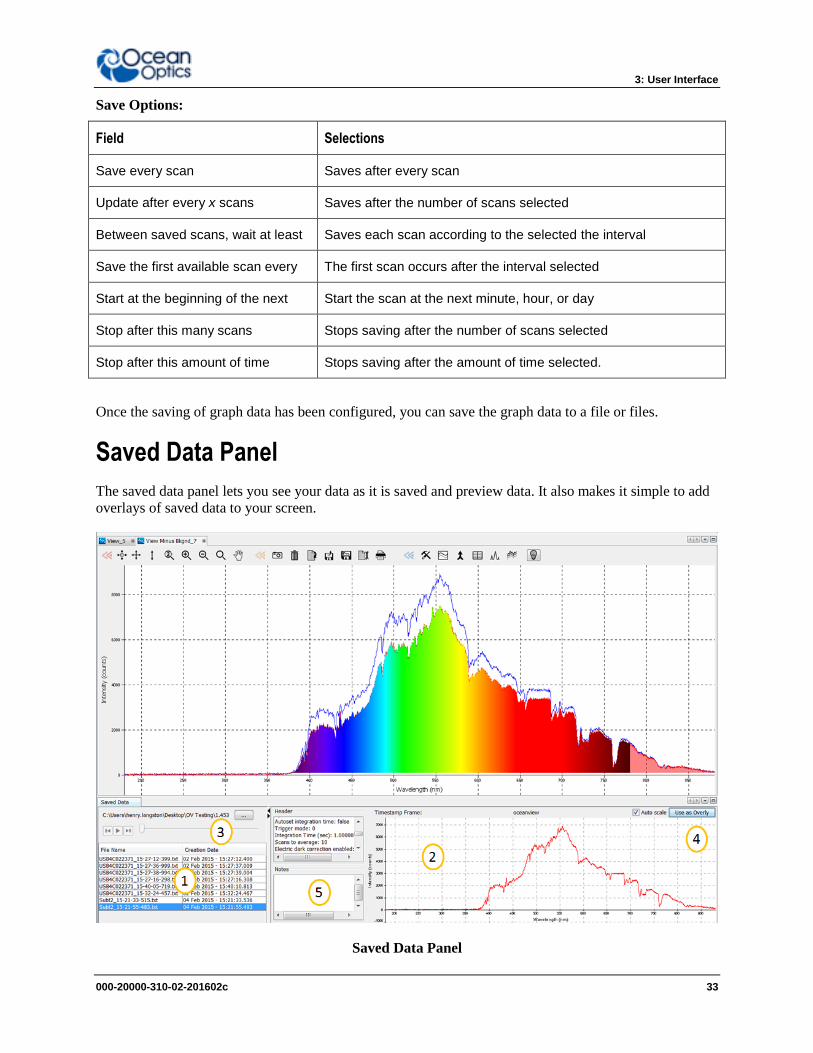
Saved Data Panel
The saved data panel lets you see your data as it is saved and preview data. It also makes it simple to add
overlays of saved data to your screen.
Saved Data Panel
3: User interface
34 000-20000-300-02-201602c
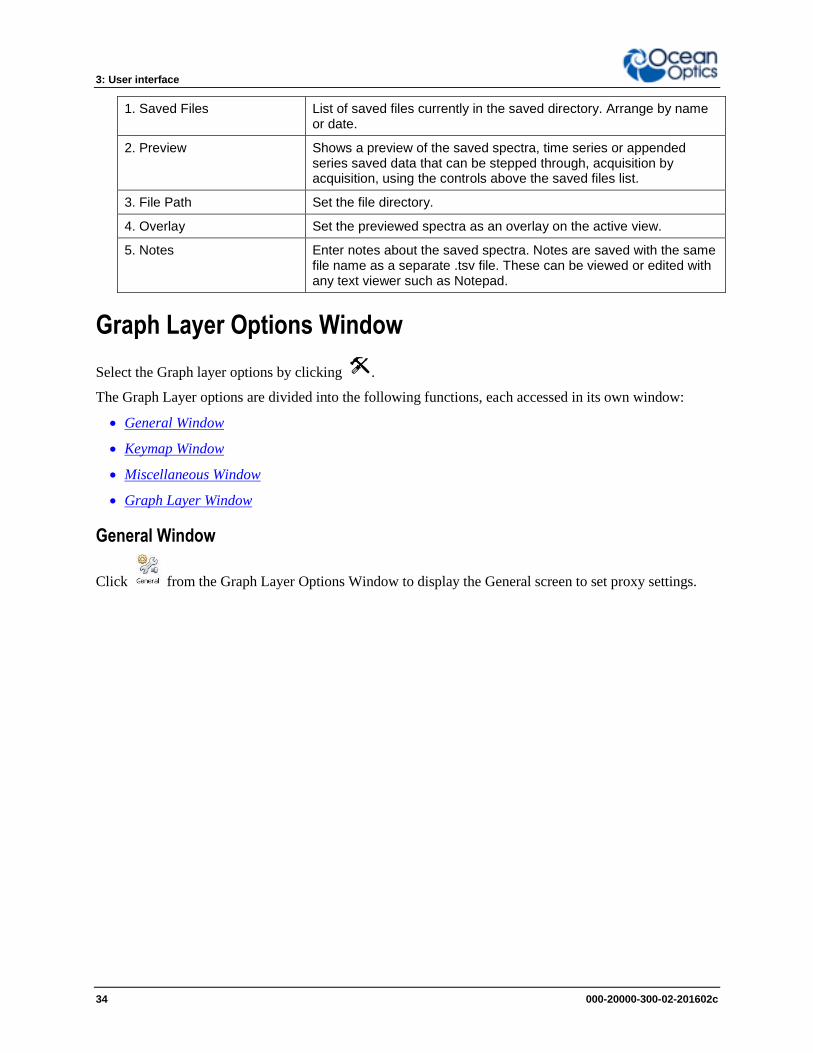
1. Saved Files List of saved files currently in the saved directory. Arrange by name or date.
2. Preview Shows a preview of the saved spectra, time series or appended series saved data that can be stepped through, acquisition by acquisition, using the controls above the saved files list.
3. File Path Set the file directory.
4. Overlay Set the previewed spectra as an overlay on the active view.
5. Notes Enter notes about the saved spectra. Notes are saved with the same file name as a separate .tsv file. These can be viewed or edited with any text viewer such as Notepad.
Graph Layer Options Window
Select the Graph layer options by clicking .
The Graph Layer options are divided into the following functions, each accessed in its own window:
General Window
Keymap Window
Miscellaneous Window
Graph Layer Window
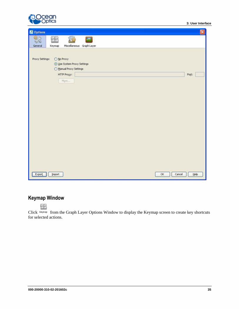
General Window
Click from the Graph Layer Options Window to display the General screen to set proxy settings.
3: User Interface
000-20000-310-02-201602c 35
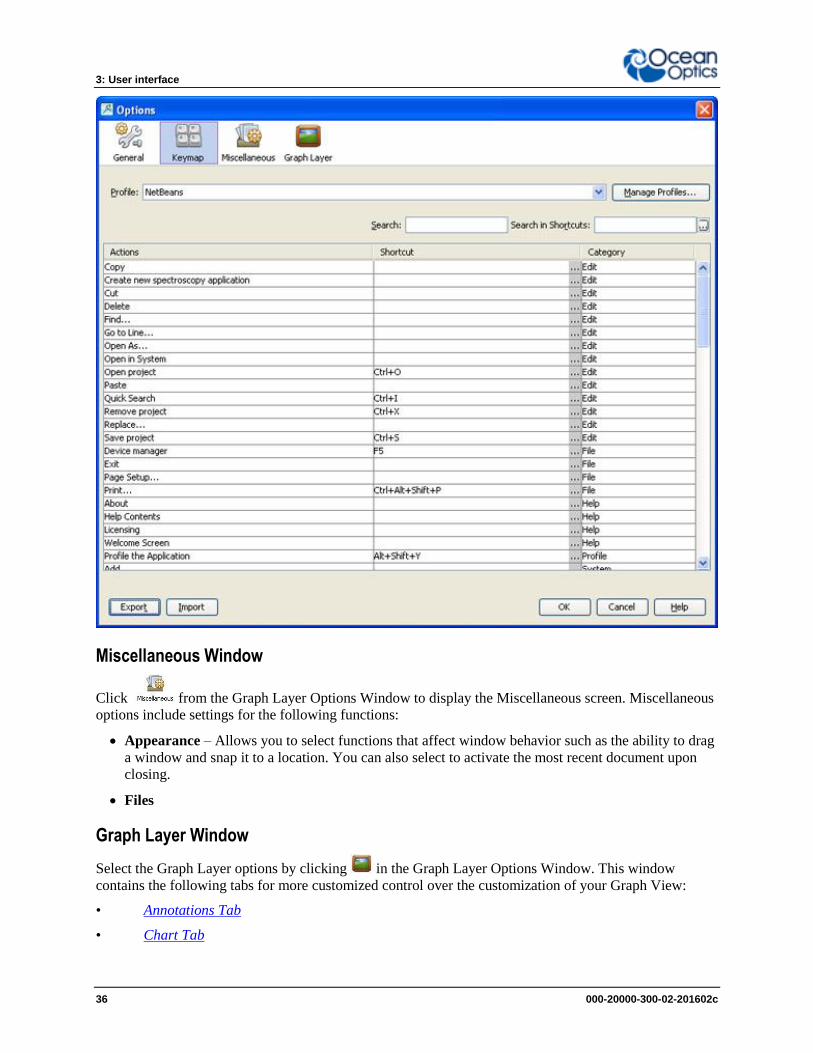
Keymap Window
Click from the Graph Layer Options Window to display the Keymap screen to create key shortcuts
for selected actions.
3: User interface
36 000-20000-300-02-201602c
Miscellaneous Window
Click from the Graph Layer Options Window to display the Miscellaneous screen. Miscellaneous
options include settings for the following functions:
Appearance – Allows you to select functions that affect window behavior such as the ability to drag
a window and snap it to a location. You can also select to activate the most recent document upon
closing.
Files
Graph Layer Window
Select the Graph Layer options by clicking in the Graph Layer Options Window. This window
contains the following tabs for more customized control over the customization of your Graph View:
• Annotations Tab
• Chart Tab
3: User Interface
000-20000-310-02-201602c 37
• Visible Spectrum Tab
• Trendline Tab
• Unit Precision Tab
• Scalar Tab
Annotations Tab
This tab allows you to add text or an image to a specific location on the graph. Annotations are associated
with a specific Graph View (selectable), and when the Graph View is removed, the annotations associated
with it are also removed.
► Procedure
1. To add a new annotation on a graph,
2. Make sure Show annotation layer is selected in the Layered Properties section at the top of the
window.
3. Use the drop-down Select view menu to choose the graph for the new annotation. This drop-
down menu shows all available Graph Views.
4. Once you have selected the appropriate graph, click New Annotation and enter the desired text in
the pop-up window.
5. When finished, click OK to place the annotation in the center of the graph.
Notes
To hide a graph’s annotations without deleting them, select Hide annotation layer in the Layered
Properties box.
To adjust the position of the annotation, enter values into the Annotation position X and Y boxes
or use the up/down arrows next to the boxes. These boxes list the position of the annotation using
the same units as the current axes of the graph. If you switch the x-axis units of the graph, you
must then come back to the Annotations tab and reposition your annotation on the graph using the
Annotation position X and Y boxes.
After exiting the Graph Layer Options panel you can also move the annotation around the graph
by grabbing and dragging it by holding down the left-click button on the mouse.
Chart Tab
Modifies the appearance of the graph such as chart area, gridlines and graph axes.
Chart Area – alters the color, pattern, and width of the gridlines on the graph. The gridlines for the
X and Y axes can be toggled on or off using the appropriate Set gridlines check boxes. Adjust the
colors of the gridlines and the background chart area with the Gridline Color and Chart Area
Color boxes. Click either of these buttons to open a Color Selection window to choose the color of
the chart or grid lines using a set of predetermined color swatches, by adjusting Hue, Saturation, and
Brightness color values (HSB), or by choosing Red, Green, and Blue color coordinates (RGB). A
preview of the new color is shown in the Preview section.
3: User interface
38 000-20000-300-02-201602c
Axes Area – alters the size, style, and spacing of the axis labels and values. The fields beginning
with “Label” control the appearance of the axis quantity and units. The fields beginning with “Tick
Mark” control the numerical X and Y axis values. The Increase and Decrease buttons increase or
decrease the spacing between adjacent numerical values on the X or Y axis.
Visible Spectrum Tab
Overlays a colored, graphical representation of the visible spectrum of light onto any OceanView graph.
Layer Properties – shows or hides the visible overlay as well as extends the overlay past the visible
(380 nm to 780 nm) into the ultraviolet and infrared regions of the graph. To enable either the UV or
the IR regions of the spectrum, check the appropriate boxes in this section.
Visible Spectrum Properties – adjusts how and where the visible spectrum will be displayed.
- Display the visible overlay as a bar located at the x-axis of the graph by selecting Show
Visible Spectrum as Bar in X Axis. The visible overlay remains clipped to the x-axis
regardless of the spectral activity. Or select Clip Visible Spectrum to Trendline for the visible
overlay to fill in the section between the spectral trend line and the x-axis. The visible overlay
rises and falls as the light intensity changes.
- Check the Invert box to fill in the section between the spectral trend line and the top of the
graph. The visible overlay will still grow and shrink as the light intensity changes, although
this time in the opposite direction.
Trend Line Selection – allows you to choose which spectral trend line the visible overlay will be
clipped to. If only one trend line is fed into the graph, then this section is blank. If two or more trend
lines are displayed on the graph, a selection table appears in this section. Choose the spectral trend
line that will control the visible overlay by clicking on the appropriate row in the table. There will be
no change in the display if the visible overlay is shown as a bar on the x-axis.
Trendline Tab
Allows you to change the colors that OceanView uses to display the spectral trend lines and overlays for
each graph.
► Procedure
1. Click and hold on the color(s) you want to change (up to 20), then drag the cursor around the pop-
up window to the desired hue for the selected color.
2. Click Reset Colors to reset the trendline color to the default shade.
3. Select the desired line width.
4. Select the number of trendline trails to include on the graph and the number between scans.
5. When you are satisfied with your selections, click OK to finish.
Unit Precision Tab
Allows you to specify the precision reported for the wavelength and intensity. You can also set the X and
Y axis range and select the units reported on the X axis.
Range Precision – alters the precision and visual display of data used in calculations. OceanView
rounds the data to the value set in the X Axis decimal places and Y Axis decimal places boxes.
Due to space limitations, the X and Y axes will not alter to display more digits on the graph. You can
see the change when data is saved to a file or copied and pasted into an outside program. The change
3: User Interface
000-20000-310-02-201602c 39
in the number of displayed digits is also shown with data in the Scalar View. To adjust the number of
decimal place digits that are displayed in a Scalar View, change the value in the Y Axis decimal
places box. Check the Use scientific notation box to copy, save, and display the appropriate data in
scientific notation.
Axis Range – saves a set of customized values that you can use to quickly rescale your graph to a
default range. The axis values entered here can be applied when you click Use ‘Options’ setting in
the View Properties Dialog Box. The values entered in this section of the Unit Precision tab
populate the display boxes of the View Properties Dialog Box. You must click Apply and then Exit
in View Properties Dialog Box to rescale the graph to the desired values.
Scalar Tab
Allows you to set the font size, style, and color for Scalar View windows.
► Procedure
1. To set the background color or font color,
2. Click and hold the left mouse button over the color you wish to alter. This will open a color
selection window.
3. Move the mouse cursor over the color you wish to use and release the left mouse button.
4. When you are finished making changes, click Apply to update the Scalar View.
Menus OceanView provides the following menus located at the top of the screen:
File Menu
Window Menu
Help Menu
File Menu
The File menu consists of the following menu selections:
Create New Spectroscopy Application
Open Project
Save Project
Tools
Start All File Writers
Page Setup
Exit
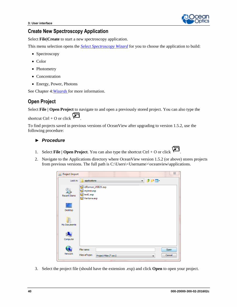
3: User interface
40 000-20000-300-02-201602c
Create New Spectroscopy Application
Select File|Create to start a new spectroscopy application.
This menu selection opens the Select Spectroscopy Wizard for you to choose the application to build:
Spectroscopy
Color
Photometry
Concentration
Energy, Power, Photons
See Chapter 4:Wizards for more information.
Open Project
Select File | Open Project to navigate to and open a previously stored project. You can also type the
shortcut Ctrl + O or click .
To find projects saved in previous versions of OceanView after upgrading to version 1.5.2, use the
following procedure:
► Procedure
1. Select File | Open Project. You can also type the shortcut Ctrl + O or click .
2. Navigate to the Applications directory where OceanView version 1.5.2 (or above) stores projects
from previous versions. The full path is C:\Users\<Username>\oceanview\applications.
3. Select the project file (should have the extension .exp) and click Open to open your project.
3: User Interface
000-20000-310-02-201602c 41
Save Project
Select File | Save Project to save a project in a location that you specify You can also click .
Tools
Select File | Tools to display the Tools menu to choose from the following selections:
Combine Calibration – This feature allows you to combine two spectrometer calibration files
that you have created; one file using a calibrated deuterium lamp source (UV) and the other
using a calibrated tungsten lamp source (VIS). This will result in a spectrometer calibration file
that can be used across the entire spectral range.
► Procedure
1. Select File | Tools | Combine Calibration.
2.Enter the file name of the spectrometer calibration file you created with the deuterium lamp
source or browse to the desired file.
2. Enter the file name of the spectrometer calibration file that you created with a tungsten lamp
source or browse to the desired file.
3. In the Boundary Wavelength field, select the wavelength at which point the two files will be
joined or go on to Step 5 to just accept the value provided by OceanView.
4. Click . The graph of the combined files appears in the Spectrometer Calibration
Preview.
Raw USB – This is password-protected area providing raw read/write USB capability.
OceanView always acts as the master (in terms of initiating writes). The device returns with the
results.
Start all file writers
Select File | Start for all file writers to start saving all previously configured graph view saves at once.
Single graph views are saved by clicking .
Page Setup
Select File | Page Setup… to display the Page Setup dialog box to allow you to set printing parameters.
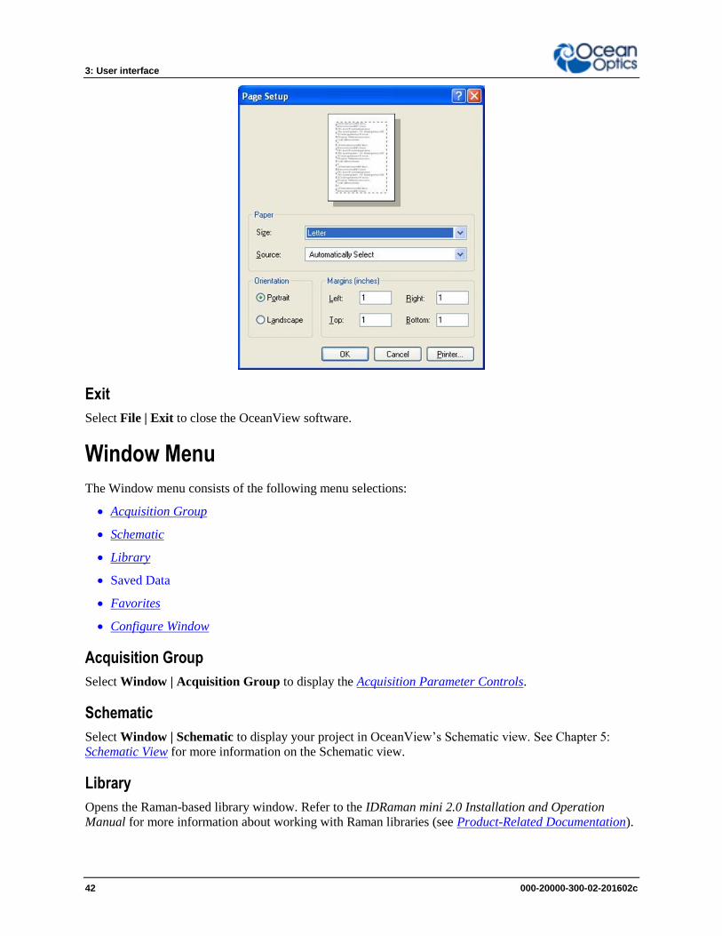
3: User interface
42 000-20000-300-02-201602c
Exit
Select File | Exit to close the OceanView software.
Window Menu
The Window menu consists of the following menu selections:
Acquisition Group
Schematic
Library
Saved Data
Favorites
Configure Window
Acquisition Group
Select Window | Acquisition Group to display the Acquisition Parameter Controls.
Schematic
Select Window | Schematic to display your project in OceanView’s Schematic view. See Chapter 5:
Schematic View for more information on the Schematic view.
Library
Opens the Raman-based library window. Refer to the IDRaman mini 2.0 Installation and Operation
Manual for more information about working with Raman libraries (see Product-Related Documentation).
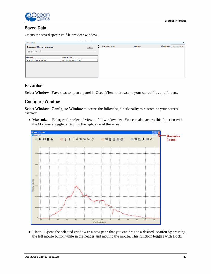
3: User Interface
000-20000-310-02-201602c 43
Saved Data
Opens the saved spectrum file preview window.
Favorites
Select Window | Favorites to open a panel in OceanView to browse to your stored files and folders.
Configure Window
Select Window | Configure Window to access the following functionality to customize your screen
display:
Maximize – Enlarges the selected view to full window size. You can also access this function with
the Maximize toggle control on the right side of the screen.
Float – Opens the selected window in a new pane that you can drag to a desired location by pressing
the left mouse button while in the header and moving the mouse. This function toggles with Dock.
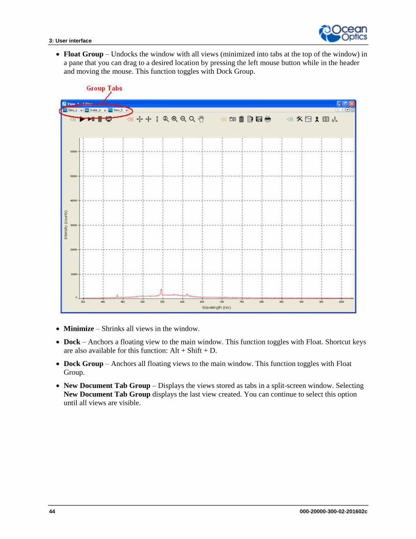
3: User interface
44 000-20000-300-02-201602c
Float Group – Undocks the window with all views (minimized into tabs at the top of the window) in
a pane that you can drag to a desired location by pressing the left mouse button while in the header
and moving the mouse. This function toggles with Dock Group.
Minimize – Shrinks all views in the window.
Dock – Anchors a floating view to the main window. This function toggles with Float. Shortcut keys
are also available for this function: Alt + Shift + D.
Dock Group – Anchors all floating views to the main window. This function toggles with Float
Group.
New Document Tab Group – Displays the views stored as tabs in a split-screen window. Selecting
New Document Tab Group displays the last view created. You can continue to select this option
until all views are visible.
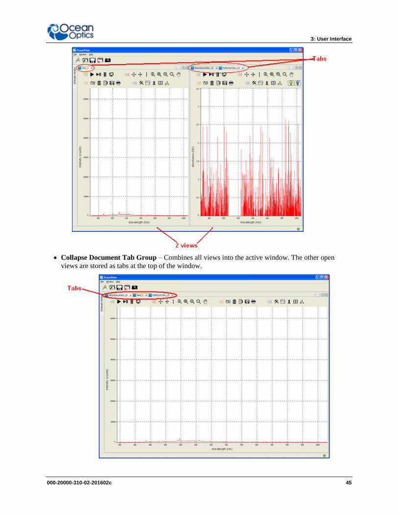
3: User Interface
000-20000-310-02-201602c 45
Collapse Document Tab Group – Combines all views into the active window. The other open
views are stored as tabs at the top of the window.
3: User interface
46 000-20000-300-02-201602c
Help Menu
The Help menu consists of the following menu selections:
Welcome Screen
Licensing – Allows you to register your product. Also displays the software build date.
Help Contents – Displays the full content of the OceanView help file
Check for Updates – Connects to the Ocean Optics site to check for any updates to your
OceanView software. OceanView software features one year of free web-based, automatic upgrades
when you buy the software.
About – Displays certain software and system specifications.
000-20000-310-02-201602c 47
Chapter 4
Wizards
Overview OceanView provides you with a wealth of functionality to capture, store and process your data. This
chapter contains descriptions of wizards and other functionality. Also see Chapter 3: User Interface for
more information on the menus and control buttons available on the OceanView user interface.
Select File |Create new spectroscopy application or click the Create new spectroscopy application icon
to access the wizards.
Select Data Source Wizard Selects the spectrometer to be used for the chosen wizard. When multiple devices are present, the selected
one is shown in blue.
Set Acquisition Parameters Wizard
Sets the spectrometer measurement parameters and controls before any data capture occurs in the
wizards. The panel has two tabs:
Main Controls – Set the basic and advanced features of the attached spectrometer. The Automatic
button in the Integration Time control box automatically adjusts the spectrometer’s integration time
to bring the highest point of the signal to 85% of full saturation value. This value is represented by
the horizontal blue line on the preview graph.
The integration time may also be set manually by using the numeric spinner control and the drop-
down units menu. Note that the Nonlinearity Correction control is grayed out until the Electric
Dark control is enabled. Also note that once a triggering mode for the spectrometer has been set, the
device will wait for an external trigger before continuing. It will appear as though the spectrometer
has locked up and no further data acquisitions will occur until the External Trigger pin on the device
receives a signal.
Caution
If you have accidentally entered a trigger mode without an external trigger available, you
must disconnect and reconnect the spectrometer to continue.
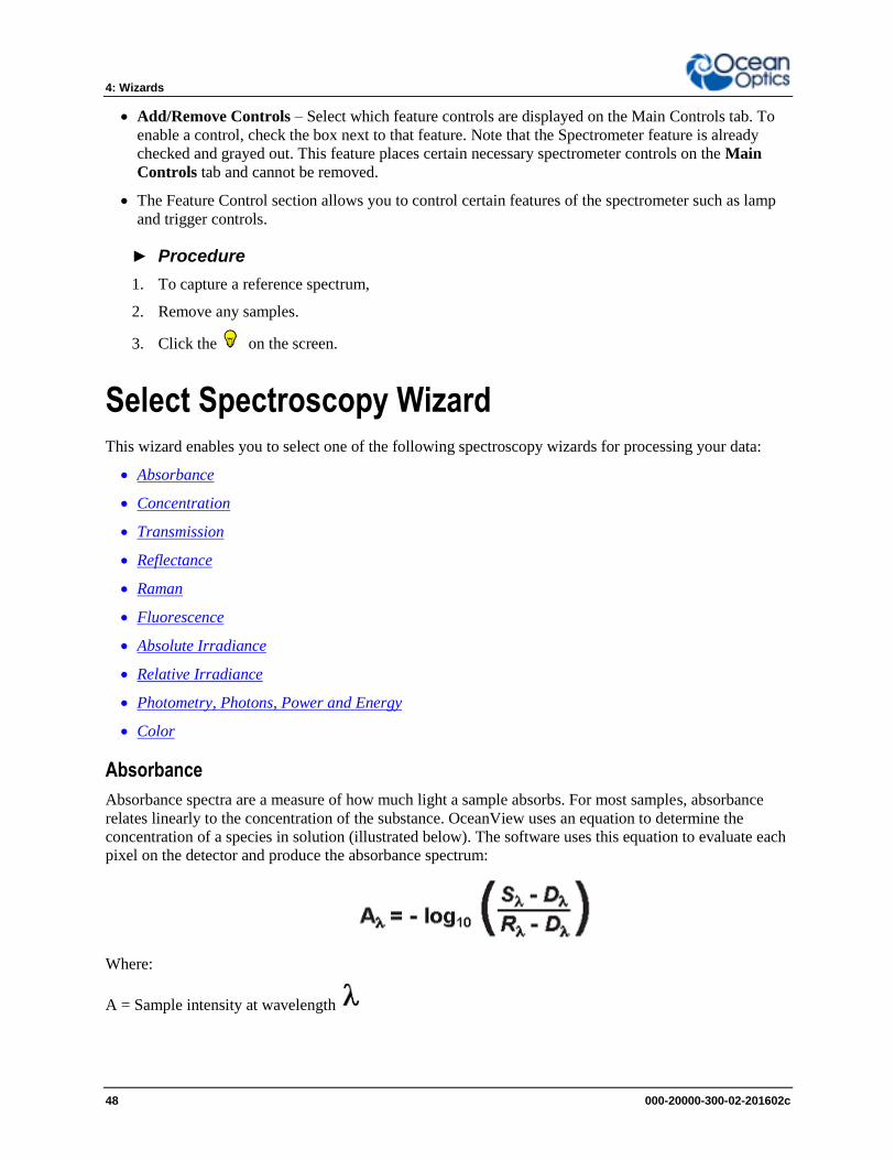
4: Wizards
48 000-20000-300-02-201602c
Add/Remove Controls – Select which feature controls are displayed on the Main Controls tab. To
enable a control, check the box next to that feature. Note that the Spectrometer feature is already
checked and grayed out. This feature places certain necessary spectrometer controls on the Main
Controls tab and cannot be removed.
The Feature Control section allows you to control certain features of the spectrometer such as lamp
and trigger controls.
► Procedure
1. To capture a reference spectrum,
2. Remove any samples.
3. Click the on the screen.
Select Spectroscopy Wizard This wizard enables you to select one of the following spectroscopy wizards for processing your data:
Absorbance
Concentration
Transmission
Reflectance
Raman
Fluorescence
Absolute Irradiance
Relative Irradiance
Photometry, Photons, Power and Energy
Color
Absorbance
Absorbance spectra are a measure of how much light a sample absorbs. For most samples, absorbance
relates linearly to the concentration of the substance. OceanView uses an equation to determine the
concentration of a species in solution (illustrated below). The software uses this equation to evaluate each
pixel on the detector and produce the absorbance spectrum:
Where:
A = Sample intensity at wavelength
4: Wizards
000-20000-310-02-201602c 49
D = Background intensity at wavelength
R = Reference intensity at wavelength
The concentration of a species in a solution directly affects the absorbance of the solution. This
relationship, known as Beer’s Law, is expressed as:
Where:
A = Absorbance at wavelength ,
= Extinction coefficient of the absorbing species at wavelength
c = Concentration of the absorbing species and l is the optical path length of the absorption.
► Procedure
1. Invoke the Absorbance wizard from the Spectroscopy Application Wizards screen on the
Welcome screen or by clicking the Create new spectroscopy application icon .
2. Select Absorbance only.
3. Set Acquisition Parameter controls.
4. Store Reference spectrum.
5. Store Background spectrum.
Concentration
Concentration is the amount of a specified substance in a solution. Graphs of absorbance vs.
concentration are known as Beer’s Law plots. These are prepared by measuring the light absorbed by a
series of solutions with different known concentrations.
The length of the sample, such as the path length of our cuvette holder, and the wavelength chosen for
monitoring the amount of light absorbed are constants. A linear plot from taking scans of these standard
solutions with known concentrations is then obtained. The plot is then used to determine the unknown
concentrations of substances in solutions.
► Procedure
1. Invoke the Concentration wizard from the Spectroscopy Application Wizards screen on the
Welcome screen or by clicking the Create new spectroscopy application icon .
2. Select Concentration.
3. Choose between two different concentration models:
a. Beer-Lambert Law -- Use this model when you know the Molar Extinction Coefficient
( ) and Path Length (l) of the unknown solution.
4: Wizards
50 000-20000-300-02-201602c
b. Calibrate from solutions of known concentration using a series of known solutions
4. Use the Existing Absorbance panel to select the absorbance process used to calculate the
concentration data.
c. If no absorbance process already exists, select New to begin. You will complete the steps
for the Absorbance wizard before being brought back to complete the Concentration
wizard.
d. If an Absorbance wizard has already been run, select it under Select existing
Absorbance process.
Beer's Law
5. Use the Beer's Law panel to set the parameters for your Beer-Lambert concentration
experiment.
a. The Wavelength box determines at what wavelength the absorbance will be
evaluated. The concentration based on absorbance at this wavelength will be displayed in
a scalar window upon completion of the wizard.
b. Concentration Units allows you to enter in the appropriate units for display in the scalar
window. Note that the units for the Molar Extinction Coefficient units will update when
you click off of this box.
c. Molar Extinction allows you to enter the Molar Extinction Coefficient of your
solution. Note that the units on this coefficient are set by the previous box. For your
final concentration to be displayed correctly, the Molar Extinction Coefficient must be
converted to the appropriate units.
d. Path Length allows you to enter the path length of the sample holder used in your
concentration experiment. Note that the units of path length default to centimeters and
cannot be changed.
e. Compound Name allows you to set the name of the solution used in your concentration
experiment. This name will be displayed in the scalar window upon completion of the
wizard.
6. Click Finish to complete and exit the wizard.
--OR--
Known Solutions
5. Use Calibrate from solutions of known concentration to calibrate your concentration
experiment using solutions of known concentration.
- If you have a valid concentration file from a previous experiment that you would like to use,
click Load File and select the appropriate .con file. The file will populate all necessary fields.
- --OR--
- If you are beginning a new experiment, begin by entering the Compound Name and
Concentration Units in the boxes at the top of the panel. The Notes box is convenient for
capturing any comments pertaining to the experiment.
a. Build a table of known concentration and absorbance values. Begin by placing a sample
of known concentration in the sample holder.
b. Enter the sample’s concentration in the Concentration box.

4: Wizards
000-20000-310-02-201602c 51
c. Click Get Absorbance. Note that you may need to click Get Absorbance twice to get
an accurate value.
d. When you are satisfied with the absorbance value for the given concentration, click Add
Sample Point to add the values to the data table.
e. Remove the sample and place a sample with a different concentration in the sample
holder.
f. Repeat the above steps C -- E for all of your known sample concentrations.
g. Note that the graph in the lower left corner of the panel populates each new data point
that is added and shows the trend line that best fits your data. If you need to remove a
point from the data table, click on that row in the table to highlight it and then click
Remove Sample Point. This point will be removed from the table and the graph.
6. Use the Regression box in the lower right corner of the panel to select between a first order
(linear) regression and a second order (quadratic) regression.
a. The Zero Intercept check box will force the trend line to pass through the point 0,0 if
selected.
b. If the Zero Intercept check box is not selected, the regression will use only the points
listed in the above data table.
7. Click Save File near the top of this panel to save your data in a new concentration (.con) file that
can be used to quickly set up this experiment in the future.
8. Click Finish to complete and exit the wizard.
Transmission
Transmission is the percentage of energy passing through a sample relative to the original reference
amount. This is also the spectral processing mode used for reflection spectroscopy, as the math necessary
to compute reflection is identical to that required for transmission. The wizard leads you to first store
reference and background spectra before you can access Transmission mode.
OceanView calculates the transmission of a solution using the following equation:
Where:
= Sample intensity at wavelength
= Background intensity at wavelength
= Reference intensity at wavelength
► Procedure
1. Invoke the Transmission wizard from the Spectroscopy Application Wizards screen on the
Welcome screen or by clicking the Create new spectroscopy application icon .
2. Select either an active acquisition or start a new one.
4: Wizards
52 000-20000-300-02-201602c
3. Set Acquisition Parameter controls.
4. Store Reference spectrum.
5. Store Background spectrum.
Reflectance
Reflectance is the return of radiation by a surface, without a change in wavelength. Reflection mode is
also the spectral processing mode used for transmission spectroscopy, as the math necessary to compute
transmission is identical to that required for reflectance.
Follow the wizard to take reference and background spectra before you can access Reflection mode.
OceanView calculates the reflection of a solution using the following equation:
Where:
= Sample intensity at wavelength
= Background intensity at wavelength
= Reference intensity at wavelength
► Procedure
1. Invoke the Reflectance wizard from the Spectroscopy Application Wizards screen on the
Welcome screen or by clicking the Create new spectroscopy application icon .
2. Select either an active acquisition or start a new one.
3. Set Acquisition Parameter controls.
4. Store Reference spectrum.
5. Store Background spectrum.
Raman
► Procedure
1. Invoke the Raman wizard from the Spectroscopy Application Wizards screen on the Welcome
screen or by clicking the Create new spectroscopy application icon .
2. Select either an active acquisition or start a new one.
3. Set Acquisition Parameter Controls.
4. Configure Raman:
a. Store Background spectrum.
b. Set the laser wavelength. This value allows the x-axis of the final graph to be converted
to wavenumbers expressed in inverse centimeters.
4: Wizards
000-20000-310-02-201602c 53
c. Enter the correct laser wavelength (in nm) and then click Apply.
Fluorescence
A fluorescence measurement is a type of relative irradiance measurement in which the energy given off
by materials excited by light at shorter wavelengths is measured. Advantages of fluorescence include high
sensitivity, high speed (intensity changes on the order of picoseconds), and safety (nondestructive to
sample and no hazardous by-products).
► Procedure
1. Invoke the Quick View Fluorescence wizard from the Spectroscopy Application Wizards screen
on the Welcome screen or by clicking the Create new spectroscopy application icon .
2. Select either an active acquisition or start a new one.
3. Set the Acquisition Parameter controls.
4. Store a Background spectrum.
Absolute Irradiance
Irradiance is the amount of light present on a particular area, such as the fiber’s cross-section at its tip, a
cosine corrector’s surface (CC-3 and CC-3-UV have a diameter of 3900, while the CC-3-DA is 7140), or
the integrating sphere’s surface (measures the total optical output of a light source inserted into the
integrating sphere).
Absolute Irradiance Mode calculates the true irradiance of a spectrum, displayed in actual uW/cm^2/nm
(or uW/nm when using an integrating sphere) incident on the probe’s collection area. You do not need to
store reference spectrum first since absolute irradiance is not relative to another measurement. However,
you must store a background spectrum and have a calibration file before you can measure absolute
irradiance.
If your spectrometer was calibrated by Ocean Optics, you should have received a CD containing the
Radiometric Calibration Files specific to your spectrometer. If you have these files, select Get Irradiance
Calibration from File.
If you do not have these files, select New Calibration to create your own spectrometer calibration files
using calibrated light sources that have known spectral output (microwatts per square centimeter per
nanometer).
► Procedure
1. Invoke the Absolute Irradiance wizard from the Spectroscopy Application Wizards screen on the
Welcome screen or by clicking the Create new spectroscopy application icon .
2. Select either an active acquisition or start a new one.
3. Select the calibration source to begin the irradiance calibration of your spectrometer:
- Get Irradiance Calibration from File: Loads a previous irradiance calibration using an
existing .cal or OOIIrrad.cal file.
- New Calibration: Creates a new irradiance calibration for the spectrometer using a calibrated
light source and associated lamp file (.lmp). This option also allows you to save the new
calibration as a .cal file that can be loaded at a later time.
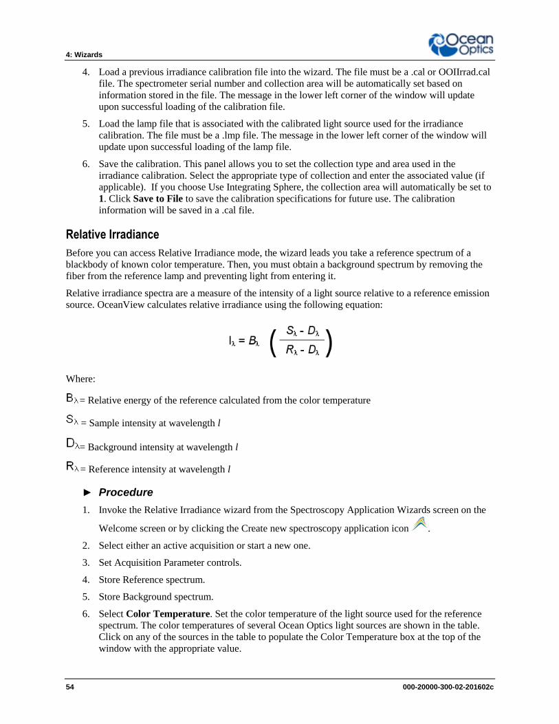
4: Wizards
54 000-20000-300-02-201602c
4. Load a previous irradiance calibration file into the wizard. The file must be a .cal or OOIIrrad.cal
file. The spectrometer serial number and collection area will be automatically set based on
information stored in the file. The message in the lower left corner of the window will update
upon successful loading of the calibration file.
5. Load the lamp file that is associated with the calibrated light source used for the irradiance
calibration. The file must be a .lmp file. The message in the lower left corner of the window will
update upon successful loading of the lamp file.
6. Save the calibration. This panel allows you to set the collection type and area used in the
irradiance calibration. Select the appropriate type of collection and enter the associated value (if
applicable). If you choose Use Integrating Sphere, the collection area will automatically be set to
1. Click Save to File to save the calibration specifications for future use. The calibration
information will be saved in a .cal file.
Relative Irradiance
Before you can access Relative Irradiance mode, the wizard leads you take a reference spectrum of a
blackbody of known color temperature. Then, you must obtain a background spectrum by removing the
fiber from the reference lamp and preventing light from entering it.
Relative irradiance spectra are a measure of the intensity of a light source relative to a reference emission
source. OceanView calculates relative irradiance using the following equation:
Where:
= Relative energy of the reference calculated from the color temperature
= Sample intensity at wavelength l
= Background intensity at wavelength l
= Reference intensity at wavelength l
► Procedure
1. Invoke the Relative Irradiance wizard from the Spectroscopy Application Wizards screen on the
Welcome screen or by clicking the Create new spectroscopy application icon .
2. Select either an active acquisition or start a new one.
3. Set Acquisition Parameter controls.
4. Store Reference spectrum.
5. Store Background spectrum.
6. Select Color Temperature. Set the color temperature of the light source used for the reference
spectrum. The color temperatures of several Ocean Optics light sources are shown in the table.
Click on any of the sources in the table to populate the Color Temperature box at the top of the
window with the appropriate value.
4: Wizards
000-20000-310-02-201602c 55
Photometry, Photons, Power and Energy
This wizard enables you to take photometry measurements such as luminous flux (lumen), illuminance
(lux), and luminous intensity (candela). Photopic/Scotopic values are calculated over a 380 to 780 nm
wavelength range. Scotopic conditions are defined when the luminance is between 10-2 and 10-6 of a
candela per square meter (cd/m2). The difference between this scotopic vision (low-level condition)
compared to a photopic (high-level condition) affects the calculations for luminous flux (lumen),
illuminance (lux), and luminous intensity (candela) by using the V’( ) scotopic luminosity
function instead of the V( ) photopic luminosity function.
This wizard also enables you to measure integrated intensities. Radiometric values require that you
specify the wavelength range.
► Procedure
1. Invoke the Photometry, Photons, Power and Energy wizard from the Spectroscopy Application
Wizards screen on the Welcome screen or by clicking the Create new spectroscopy application
icon ( ).
2. Select the absolute irradiance process used to calculate the Photometry, Photons, Power and
Energy data.
a. If an absolute irradiance wizard has already been run, you can select it with Get
Calibration from File or Get Irradiance Calibration from Spectrometer.
--OR--
b. If no absolute irradiance process already exists, select New Calibration to begin.
3. Follow the remaining steps in the wizard to get the desired data.
Color
With OceanView, you can calculate and report the Color Rendering Index (CRI) and Correlated Color
Temperature (CCT) for your samples. OceanView will compute all color measurements except RGB.
Emissive color measurements – Require a spectrometer, which has been calibrated to take
irradiance readings (either relative or absolute). OceanView gives you the option of choosing to
measure either emissive or reflective color from either absolute or relative irradiance.
Reflective color measurements – Do not require an irradiance calibration, but they do require a
reference spectrum. This reference scan is taken with the same optical configuration, except a
perfect reflector is placed at the same location as the samples.
► Procedure
1. Invoke the Color wizard from the Spectroscopy Application Wizards screen on the Welcome
screen or by clicking the Create new spectroscopy application icon .
2. In the Color Source panel, select the processing method used to calculate color data. By
choosing any of the first three options, the wizard will guide you through the steps associated
with your choice before being brought back to complete the color wizard. If there is a suitable
existing process that has already been completed, this will be available to select under the last
option, Existing processing. Select the desired process and click Next. Note that Correlated

4: Wizards
56 000-20000-300-02-201602c
Color Temperature (CCT) and Color Rendering Index (CRI) will not be available if you choose a
Percent Reflection as your processed data source.
3. In the Color Setup panel, the Display Parameters portion allows you to choose which color
values are displayed upon completion of the wizard. All applicable values will be added to a
color table for display. Note that Correlated Color Temperature (CCT) and Color Rendering
Index (CRI) will not be available if you chose Percent Reflection as your processed data source.
Peak Metrics Wizard
Create thresholds on your spectral graph to isolate peaks using the Peak Metrics Wizard.
► Procedure
1. Invoke the Configure Peak Metrics wizard by clicking the View spectrum peaks icon .
2. Use the Select Processed Node panel to choose which data node supplies the information for the
calculation of peak values. Select the desired device or node by clicking on that row in the
table. The selected source will be highlighted in blue. Click Next to proceed.
3. Use the Configure Baseline panel to subtract off any underlying spectral structures that may
obscure the peaks that you are trying to identify.
- None -- The peak finder will evaluate all peaks at any y-axis value.
--OR--
- Advanced -- Allows you to adjust the spectrum to eliminate any non-pertinent data. Advanced
activates the advanced features and the window's preview graph illustrates how the changes
affect which peaks will be evaluated. As the advanced parameters are adjusted, the preview
spectrum in the graph changes position. Only peaks visible above the preview graph's x-axis
will be evaluated by the peak finder.
- Use the Horizontal threshold adjustment when your data has a relatively flat baseline
structure with protruding peaks (like the spectrum of an Ocean Optics HG-1 mercury line light
source). The value entered into the horizontal threshold box is subtracted off the y-axis value of
each pixel. As the horizontal threshold value gets larger, the preview spectrum drops closer to
the x-axis and fewer peaks will be analyzed.
- Curve fit regression attempts to eliminate any underlying base structure by subtracting off a
best fit polynomial from the spectrum. This is useful when there is an underlying curve with
superimposed peaks. An Ocean Optics PX-2 pulsed xenon light source is a good example of a
blackbody curve with protruding atomic emission peaks. In order to eliminate the underlying
blackbody structure and expose the emission peaks, a curve fit regression can be used to match
and subtract the blackbody shape. A curve fit regression of order 0 subtracts a constant that
best fits the data (the average). A first order polynomial subtracts off a straight line that best
fits the data. A second order regression subtracts off a parabola that most closely matches the
data shape. As the order number increases, the underlying curve is more closely matched and
subtracted away, leaving only the sharper peaks.
4. Click Next after selecting the desired settings.
5. Use the Peak Finder panel to characterize which of the remaining spectral features should be
evaluated. Different methods of peak analysis may be used as well as different filtering options to
reduce unwanted noise effects. The preview graph at the bottom of this panel displays the
adjusted spectrum from the previous panel.

4: Wizards
000-20000-310-02-201602c 57
c. There are two peak finding methods available:
Local Maxima -- searches for all of the local maxima that fall within the user-defined
search parameters established in the previous wizard panel.
--OR--
Derivative -- selecting this option requires that you choose a derivative order number. A
first derivative search will locate all points where the first derivative of the spectrum is
zero (stationary points). A second derivative search will locate all points where the second
derivative of the spectrum is zero (inflection points). For either method, you must choose a
minimum peak width. This parameter, measured in nanometers, will exclude any peaks
that are narrower than the user-defined value. This is useful for eliminating small, random
fluctuations due to noise. Note that the number of peaks shown in the blue text in the
Controls section will vary based on user-defined parameters entered in the Peak Finder
and Baseline Estimation wizard panels.
d. Smoothing -- To apply spatial filtering to reduce adjacent pixel discrepancies and the
unwanted effects of noise, choose from the following:
Boxcar -- Simple boxcar filtering is a specialized case of Savitzky-Golay filtering where
the polynomial order is 0.
--OR--
Savitzky-Golay -- For a Savitzky-Golay filter, the Polynomial order number must be less
than the total number of pixels used in the filter. If the Filter Span is set to 2, the
Polynomial order number must be set to 4 or less.
--OR--
None -- To proceed without any spatial filtering.
e. Filter Span -- Be aware that the number of pixels used in the filter is actually 2n+1,
where n is the number displayed in the user-defined box. If 2 is entered in the box, for
example, a total of 5 pixels are used in the filter (2 to the left + 1 center pixel + 2 to the
right).
6. Click Next after selecting the desired settings.
7. Use the Select Displayable parameters panel to select which values will be calculated and
displayed on the graph.
8. Click the Show table of values box to display these same values in a table. Check the box next to
any values you wish to display. The Rotate text on View Graph option will change the
displayed values from a vertical orientation to a horizontal orientation on the graph.
9. Click Finish.
4: Wizards
58 000-20000-300-02-201602c
Strip Chart Wizard
OceanView allows you to use Strip Charts to track processes, perform kinetic analyses, and monitor
spectral events all as a function of time. The Strip Chart shows you how the value that you selected
appears over time. This value can be any of the following:
One pixel (a single wavelength)
A ratio of two pixels (a ratio of two wavelengths)
The average of a range of pixels
An integral calculated by one of three methods representing the area beneath the graph’s trend line
You can acquire this data using any processing mode (transmission, absorbance, etc.).
► Procedure
1. Invoke the Strip Chart wizard by clicking the Create strip chart icon .
2. Use the Source Selection panel to select the source of data for the strip chart. Data can be pulled
from different devices and different schematic nodes. Select the desired device or node by
clicking on that row in the table. The selected source will be highlighted in blue.
3. In the Wavelength Selection box, choose,
- Range Selection to chart data from a single wavelength, the average over a range of
wavelengths, or integrate over a range of wavelengths and display the result
--OR--
- Ratio of Wavelength to choose different values for the numerator and denominator
and display the ratio of the two values. When choosing the values for numerator and
denominator, select data from a single wavelength, the average over a range of
wavelengths, or integrate over a range of wavelengths.
4. Use the Update Rate panel to set the data update rate and time parameters for the strip
chart. Data can be plotted on the strip chart after every scan or every nth scan, where n is a user
selected value.
To plot data after every scan, select the first option in the window.
--OR--
To plot data after every nth scan, select the second option in the window and enter your value for n in
the active box.
5. Select how long the strip chart runs before stopping using the following buttons:
a. Click Stop after this many scans and enter a value in the active box so that the strip
chart will only run for the desired number of integration cycles before stopping.
--OR—
b. Click Stop after this amount of time and two boxes will become active. Enter a
numerical value in the active box to the left and select the desired units in the active box
to the right. Now the strip chart will only run for the specified length of time before
stopping.
4: Wizards
000-20000-310-02-201602c 59
--OR--
c. Click Never Stop so that the strip chart will continue to run without stopping.
6. Use the Wavelength Selection panel, the Select Numerator panel and the Select Denominator
panel to choose to select among the following values for the wavelength, numerator, and
denominator respectively:
a. Click the button next to One wavelength and enter the desired value to select a single
wavelength to chart. Make sure your value falls within the wavelength range of the
selected spectrometer or data node. OceanView will select the pixel that is closest to the
value entered.
--OR--
b. You may choose to display the average result from a range of wavelengths by selecting
Average from. When you select this option, two boxes become active. These boxes
represent the lower and upper wavelength values over which OceanView will compute an
average value.
--OR--
c. You may also choose to display the integrated result over a range of wavelengths by
selecting Integrate over. When you select this option, three boxes become active. The
top two boxes represent the lower and upper wavelength bounds over which OceanView
will compute an integral. The last box allows you to set the integration method. You may
choose between Rectangular, Trapezoidal, or Simpson’s Rule.
The Strip Chart offers the same functionality available with the Graph View Controls with the addition of
the Strip Chart Configure Time Control.
Strip Chart Configure Time Control
The control on the Strip Chart displays the Algorithm Parameter Controls dialog box, which allows
you to adjust the trend update rate.
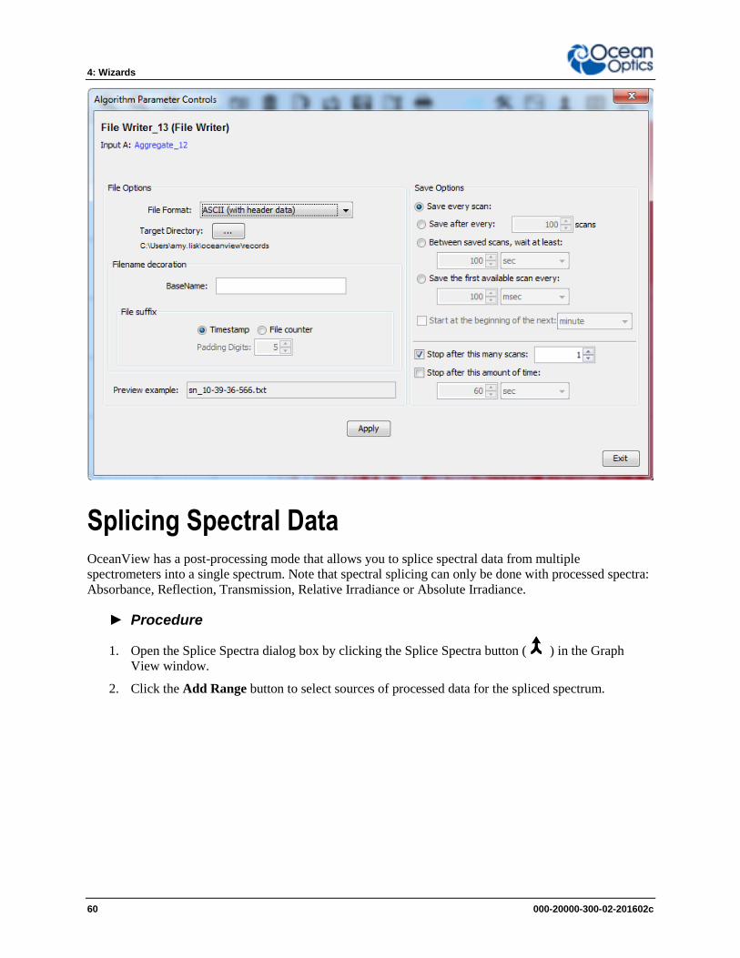
4: Wizards
60 000-20000-300-02-201602c
Splicing Spectral Data OceanView has a post-processing mode that allows you to splice spectral data from multiple
spectrometers into a single spectrum. Note that spectral splicing can only be done with processed spectra:
Absorbance, Reflection, Transmission, Relative Irradiance or Absolute Irradiance.
► Procedure
1. Open the Splice Spectra dialog box by clicking the Splice Spectra button ( ) in the Graph
View window.
2. Click the Add Range button to select sources of processed data for the spliced spectrum.
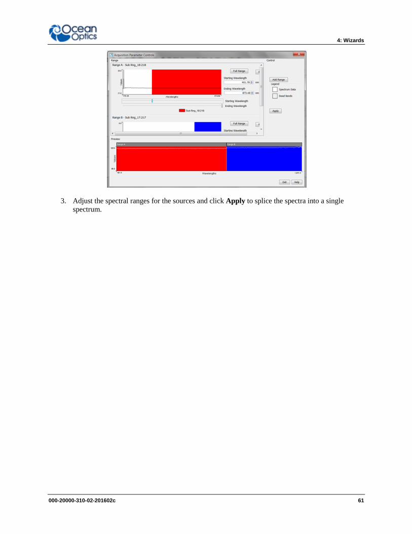
4: Wizards
000-20000-310-02-201602c 61
3. Adjust the spectral ranges for the sources and click Apply to splice the spectra into a single
spectrum.

4: Wizards
62 000-20000-300-02-201602c
000-20000-310-02-201602c 63
Chapter 5
Schematic View
Overview The Schematic View presents data from your device(s) in a diagram format with icons representing the
different devices and processes in your project as nodes and links between the nodes. In the Schematic,
you can view and manipulate the flow of data from your spectrometer through your processing steps.
Data flow is represented by the use of arrows and lines that connect different nodes. The nodes represent
points where data is processed or manipulated. The Schematic View provides you with all of the
functionality of the Window view, plus the following enhanced capabilities:
Algorithm nodes – allow for math functions such as ratios, adding multiple spectra, and adding a
constant to spectra.
Set a subrange – ability to focus on a specific subset of the spectrum
Interpolate spectral data – evenly space data from two or more spectra to analyze them
mathematically
Retrieve device properties such as serial number, firmware version, wavelength and total number of
pixels
Send a single value (such as TEC temperature, integral, average over a specific wavelength range)
from the device to the Scalar view to analyze the value over time
Preview spectra in graphs at every step in your process
Easily add new Graph and Table Views
Using the Schematic View
Spectrometers
All spectrometers detected by the software are automatically placed on the Schematic.
Add new devices to the Schematic using the Device Manager button ( ) or pressing the F5 key.
Click Rescan to scan and connect to new devices.
Double-click the spectrometer icon to open the Device Features window and view all available
device characteristics (serial number and firmware version).
5: Schematic View
64 000-20000-300-02-201602c
Acquisitions
Start a new acquisition for a spectrometer by right-clicking the spectrometer icon and selecting New
Acquisition to choose from the list of available acquisitions.
Double-click the Acquire node to open the Acquisition Parameter Controls menu and configure the
acquisition.
Adding Nodes to the Schematic: Add a data view (Graph, Scalar or Table view windows) or
processing nodes to the Schematic by right-clicking on an empty region of the Schematic and
selecting a node from the menu.
To connect nodes:
- For PC users: Hold down the Control key and left-click on the first node. While still holding
the mouse button, drag a wire from the first node to the second node. When the cursor is over
the second node, release the mouse button and the Control button: Control + Click + Drag
- For Mac users: Hold both the Shift key and the Control key while wiring a connection:
Control + Shift + Click + Drag
Double-click a node to view available feature controls and access context sensitive help.
Delete a connection between node by moving the cursor over the wire, right-clicking on it and
selecting Delete Connection. Right-click the node to Rename, Duplicate or Delete it.
Double-click a View node to go to the Data View window for that node.
If two nodes cannot be connected, OceanView will not allow you to make the connection. View the
context sensitive help for the node to determine the proper connection by double-clicking the node
and clicking the Help button.
Tip
Use the Wizards to create your Schematic and customize as desired using more than 70 algorithm
nodes.
Displaying the Schematic View When you first invoke OceanView, the Schematic View is minimized on the left side of the View
Window.
Sizing the Schematic View
The Schematic View can appear on your OceanView screen in one of three sizes as shown below:
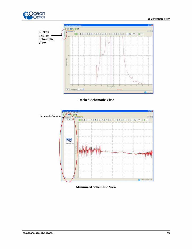
5: Schematic View
000-20000-310-02-201602c 65
Docked Schematic View
Minimized Schematic View
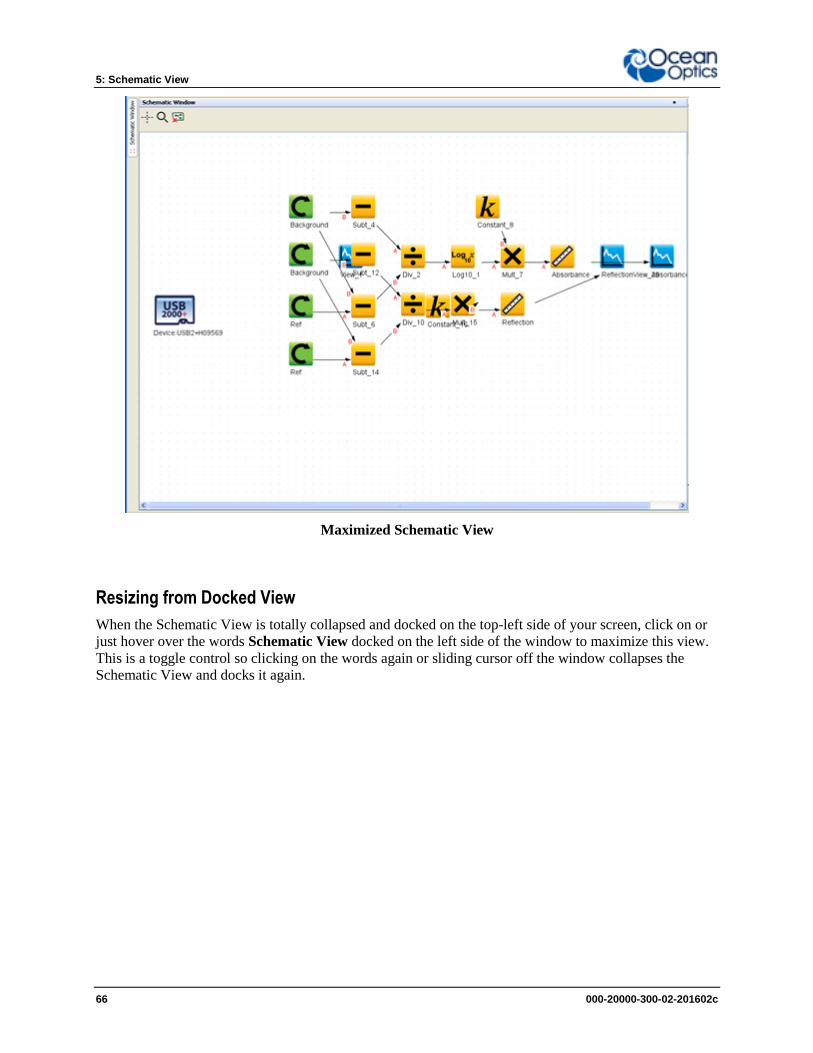
5: Schematic View
66 000-20000-300-02-201602c
Maximized Schematic View
Resizing from Docked View
When the Schematic View is totally collapsed and docked on the top-left side of your screen, click on or
just hover over the words Schematic View docked on the left side of the window to maximize this view.
This is a toggle control so clicking on the words again or sliding cursor off the window collapses the
Schematic View and docks it again.
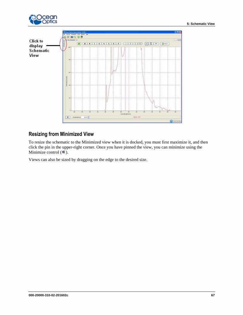
5: Schematic View
000-20000-310-02-201602c 67
Resizing from Minimized View
To resize the schematic to the Minimized view when it is docked, you must first maximize it, and then
click the pin in the upper-right corner. Once you have pinned the view, you can minimize using the
Minimize control ( ).
Views can also be sized by dragging on the edge to the desired size.
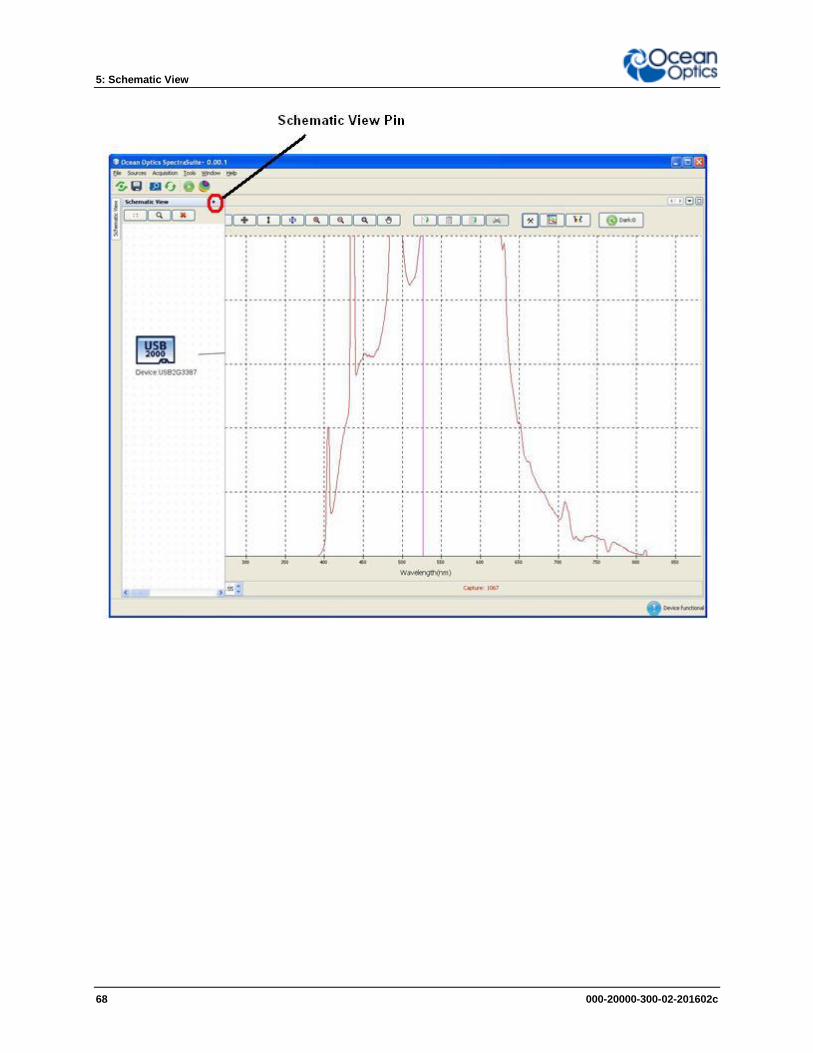
5: Schematic View
68 000-20000-300-02-201602c
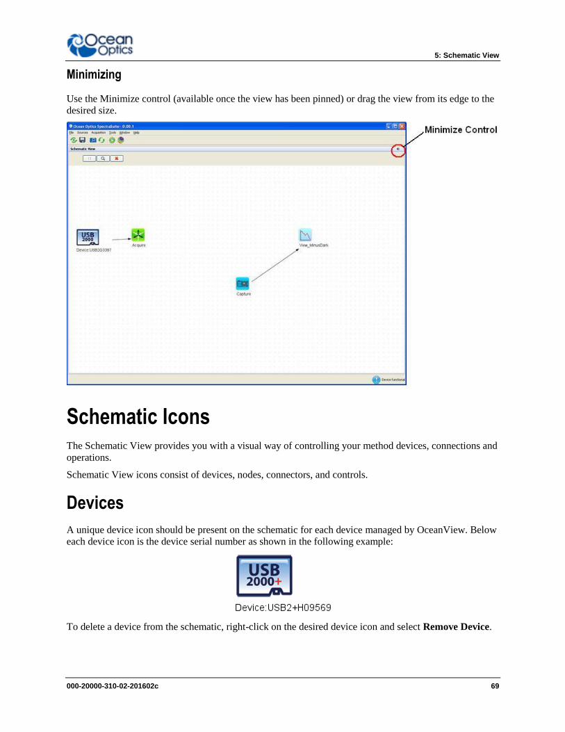
5: Schematic View
000-20000-310-02-201602c 69
Minimizing
Use the Minimize control (available once the view has been pinned) or drag the view from its edge to the
desired size.
Schematic Icons The Schematic View provides you with a visual way of controlling your method devices, connections and
operations.
Schematic View icons consist of devices, nodes, connectors, and controls.
Devices
A unique device icon should be present on the schematic for each device managed by OceanView. Below
each device icon is the device serial number as shown in the following example:
To delete a device from the schematic, right-click on the desired device icon and select Remove Device.
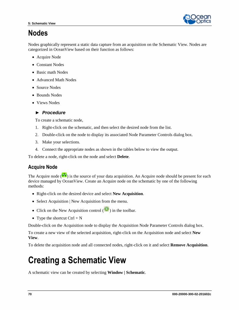
5: Schematic View
70 000-20000-300-02-201602c
Nodes
Nodes graphically represent a static data capture from an acquisition on the Schematic View. Nodes are
categorized in OceanView based on their function as follows:
Acquire Node
Constant Nodes
Basic math Nodes
Advanced Math Nodes
Source Nodes
Bounds Nodes
Views Nodes
► Procedure
To create a schematic node,
1. Right-click on the schematic, and then select the desired node from the list.
2. Double-click on the node to display its associated Node Parameter Controls dialog box.
3. Make your selections.
4. Connect the appropriate nodes as shown in the tables below to view the output.
To delete a node, right-click on the node and select Delete.
Acquire Node
The Acquire node ( ) is the source of your data acquisition. An Acquire node should be present for each
device managed by OceanView. Create an Acquire node on the schematic by one of the following
methods:
Right-click on the desired device and select New Acquisition.
Select Acquisition | New Acquisition from the menu.
Click on the New Acquisition control ( ) in the toolbar.
Type the shortcut Ctrl + N
Double-click on the Acquisition node to display the Acquisition Node Parameter Controls dialog box.
To create a new view of the selected acquisition, right-click on the Acquisition node and select New
View.
To delete the acquisition node and all connected nodes, right-click on it and select Remove Acquisition.
Creating a Schematic View A schematic view can be created by selecting Window | Schematic.
5: Schematic View
000-20000-310-02-201602c 71
► Procedure
1. The first step to using OceanView in the Schematic View is to place a spectrometer on the
schematic. Each time you start OceanView, the software looks for attached devices. Any detected
spectrometers are automatically placed on the schematic diagram.
If no device is present when you start OceanView, you will be asked if you wish to add a simulated
spectrometer. The simulated spectrometer produces a wide variety of idealized spectral data which
can be fed into different nodes for processing or viewing.
a. If no spectrometers are present on the schematic, or you wish to add an additional
spectrometer, click Device Manager at the top of the window or press the F5 shortcut
key.
b. In the Device Manager window, click Rescan and OceanView will automatically check
for USB-connected devices. If the “Automatically connect to devices” box is checked,
OceanView will add all detected spectrometers to the schematic. If the box is not
checked, all detected devices will be listed in the table.
c. To add a specific device from the list to the schematic, click on the spectrometer you
want to add and click Connect.
d. To add an Ethernet-connected device (like a Jaz spectrometer), click Add Device. In the
pop-up menu, add the IP address of the device and click Accept.
2. Once a spectrometer has been added to the schematic, an Acquisition (Acquire) node is necessary
to extract information from the device. To drop an Acquisition (Acquire) node on the schematic,
right-click on the spectrometer icon and select New Acquisition to see a list of available choices.
The type of device determines which Acquisition (Acquire) nodes are available.
3. To collect spectral data from the device, click Spectrometer. This node is automatically wired to
the spectrometer and cannot be duplicated or transferred to a different device.
4. To access and alter device features, double-click on the Acquisition (Acquire) node to open the
Acquisition Parameter Controls menu. Here you can see a graph preview and adjust various
parameters like Integration Time and Signal Averaging. These represent the basic spectrometer
controls. Add additional controls to the Main Controls tab by clicking on the Add/Remove
Controls tab and checking the boxes next to the desired feature. The controls for these features
will show up on the Main Controls tab. Unchecking a feature only hides the controls; it does not
disable that feature. The spectrometer type will determine which controls are available in the
Add/Remove Controls tab.
5. Once you have a spectrometer icon and an Acquisition (Acquire) node on your schematic, you are
ready to add data processing nodes. In OceanView, data can be static (unchanging) or dynamic
(fluctuates in time). Data can be further classified as scalar (a single value) or array (set of
values). Arrays can be one dimensional (for example, the set of wavelength values that represent
each pixel in the spectrometer) or two dimensional (the set of wavelength and intensity values for
each pixel; this is what comes out of a Spectrometer Acquisition (Acquire) node). Each schematic
node can be described by the type of data it accepts (input) and by the type of data it produces
(output). By understanding the input/output characteristics of the different nodes, you can see
how they can be wired together.
6. To place a new node on the schematic, right-click on an empty section of the schematic diagram.
A menu containing a categorized list of all available nodes pops up. Navigate through the menu
5: Schematic View
72 000-20000-300-02-201602c
and select the appropriate node by left-clicking on it. The new node will be dropped on the
schematic panel in the location where you originally right-clicked.
7. For most nodes, right-clicking on the node allows you to Rename, Duplicate, or Delete that node.
Right-clicking on an Acquire node also allows you to take a snapshot of that node. A snapshot
captures the most recent spectral acquisition and stores it within a Data Source (DataSource)
node. Right-clicking on the spectrometer icon allows you to place a variety of Acquisition
(Acquire) nodes and Output Control (Output Control) nodes (depending on the spectrometer
model). Output Control (Output Control) nodes feed data into the spectrometer allowing you to
alter its feature parameters using the schematic node data as opposed to making adjustments
through the Acquisition Parameter Controls within the Acquisition (Acquire) node.
8. To access and adjust the feature controls of any node on the schematic diagram you must double-
click on it. A window opens allowing you to view the data at that point and to make any
necessary changes. The only exceptions are the blue View nodes and the spectrometer icon.
Double-clicking on a View node exits the Schematic view and activates the Graph View window,
allowing you to see your data. Double-clicking on the spectrometer icon opens the Device
Features window, allowing you to see all available device characteristics (such as serial number
and firmware version).
9. On the schematic diagram, arrows represent the direction in which data flows. To wire a
connection between two nodes, make sure that the output data type of the first node matches the
input data type of the second node.
- For PC users, hold down the Control button and left-click on the first node. While
still holding the mouse button, drag a wire from the first node to the second node.
When the cursor is over the second node, release the mouse button and the Control
button.
- For Mac users, hold both the Shift button and the Control button while wiring a
connection.
10. If the input/output data types are incompatible, OceanView will not allow you to make the
connection. To delete a connection between nodes, move the cursor over the wire and right-click
on it. Select “Delete Connection” to erase the wire. On the OceanView schematic, solid lines
represent data that is periodically updated whereas dashed lines indicate data that is only sent one
time (like in the case of a Data Source (DataSource) node).
11. The actual location of individual nodes on the schematic diagram is purely cosmetic and nodes
can be moved around without impacting the data flow path. The connection between nodes
stretches or shrinks as well as changes direction when nodes are moved around. To change the
position of a node, move the cursor over the node and left-click and hold the mouse button down
while dragging the node to its new location.
12. Using the grid dots on the schematic can help you keep your diagram organized. To shut off the
grid dots, click in the Schematic Window toolbar.
13. As your schematic diagram grows, you may need to expand the size of the schematic window.
You can do this by dragging any node past the edge of the window and dropping it. Scroll bars
will appear at the edge of the schematic window to allow you to move around the newly enlarged
area. Once you have expanded your schematic window, you can use in the Schematic
Window toolbar to see an overview of the diagram. By dragging the gray box in the overview,
you can quickly move to any area of the schematic diagram.
5: Schematic View
000-20000-310-02-201602c 73
14. The final way to adjust the size of the schematic window is by holding down the Control key on
the keyboard and rotating the center wheel on the mouse. This will zoom the schematic window
in or out depending on which way it is turned.
15. The button clears all nodes (except the spectrometer icon) from the schematic diagram,
allowing you to start with a clean slate.
16. Once data has been acquired and processed, the end result can be displayed in the Graph View
using the blue View nodes. Spectral data can be shown by wiring it into a Graph View or Table
View node.
• Multiple spectra can be fed into one Graph View node or one Table View node for display.
• Scalar data can be displayed using a Scalar View node.
•The Color View node is used for displaying the CIE x and y color space values from a
Reflective Color (Refl Color) or Emissive Color (Emiss Color) node. Both the Scalar View and
Color View nodes can only accept one data input. Placing any of these view nodes on the
schematic will cause the associated panel to open on the Graph View window. Each of these
views has a set of controls that is accessible through the Graph View.
Order of Operations
Use the following sequence to connect nodes in the Schematic View.
► Procedure
1. Right click on the spectrometer in the schematic window and select New Output Control.
2. Select the GPIO and set up your GPIO options.
3. Connect the GPIO node to the Acquire node as shown above.
4. Call up the other nodes, sub range, subtract, and constant.
5. Enter a wavelength value in the subrange node and connect it to the Acquired node.
6. Enter a value into the constant node.
7. Connect the subrange and constant nodes to the subtract node.
8. Connect the subtract node to the GPIO node.
Icon Definitions The Schematic View Icons are described in alphabetical order below.
Absolute Value (Abs)
Outputs the absolute value of the input data.
Location: Basic Math-->Absolute Value
5: Schematic View
74 000-20000-300-02-201602c
Number of Inputs: 1
Type of Inputs: scalar or array
Type of Output: scalar or array
User Controls: N/A
Acquisition (Acquire)
Acquires data from a device and allows you to monitor and alter certain device parameters.
Location: Right-click a device icon and choose one of the options under the New Acquisition menu.
Number of Inputs: 1
Type of Inputs: device
Type of Output: Depends on the type of acquisition and the device.
User Controls: Depends on the type of acquisition and the device.
Notes: Different types of acquisitions are available for different devices. Acquisition choices may
include: Spectrometer, I²C, SPI, Board Temperature, Thermo-Electric Cooling, and Analog In. The user
controls that are available vary based on the type of acquisition selected.
Add Color View (Color)
Adds a new CIE 1931 chromaticity diagram to the View Window.
Location: Views -->Add CIE.1931 Color View
Number of Inputs: 1
Type of Inputs: EmissChrom node or ReflChrom node
Type of Output: N/A
User Controls: Planckian Locus on window view may be toggled on or off.
Notes: Click the Color node to open the Color View window. The Planckian Locus button is located in
the upper left corner of the Color View window.
Add Graph View (View)
Adds a new graph to the View Window.
5: Schematic View
000-20000-310-02-201602c 75
Location: Views -->Add Graph View
Number of Inputs: infinite
Type of Inputs: array
Type of Output: N/A
User Controls: See the Graph View window
Notes: Click the Graph View node to open the Graph View window.
Add Scalar View (Scalar)
Adds a scalar view to the View Window.
Location: Views -->Add Scalar View
Number of Inputs: 1
Type of Inputs: scalar
Type of Output: N/A
User Controls: The Configure View Parameters button in the upper left corner of the Scalar View
changes the background color, font color, font style, and font size in the Scalar tab of the options window.
Notes: Click the Scalar View node to open the Scalar View window
Add (Add)
Adds the values of inputs together.
Location: Basic Math -->Add
Number of Inputs: 2
Type of Inputs: scalar or array
Type of output: scalar or array
User Controls: Swap inputs
Aggregate (Aggregate)
Aggregates individual scalar values to display in a Table View.
Location: Advanced Math -->Filtering -->Aggregate
5: Schematic View
76 000-20000-300-02-201602c
Number of Inputs: infinite
Type of Inputs: scalar
Type of Output: Multiple scalar values
User Controls: N/A
Notes: The output of the Aggregate node must be fed into a Table View for display.
Average (Avg)
Outputs an average of an array.
Location: Basic Math -->Average
Number of Inputs: 1
Type of Inputs: array
Type of Output: scalar
User Controls: N/A
Background Estimation (Bk Est)
Removes the underlying background structure in the input spectra to reveal the desired peaks.
Location: Advanced Math -->Filtering --> Background Estimation
Number of Inputs: 1
Type of Inputs: array
Type of Output: array
User Controls: Horizontal Threshold, Curve fit regression
Notes:
As the user-defined values are altered, the spectrum in the preview graph changes shape and position.
Only pixels that display information above the x-axis of the preview graph are evaluated for peak features
when the data leaves this node.
When a value is entered in the Horizontal threshold box, that value is subtracted off the intensity values
for each pixel in the spectrum. This is useful for eliminating a relatively flat background.
The Curve fit regression box allows you to change the order number of the polynomial used to curve fit
the data. The specified polynomial order curve fit is calculated and subtracted off the spectrum.
5: Schematic View
000-20000-310-02-201602c 77
Blackbody (Blkbdy)
Outputs an ideal blackbody spectrum.
Location: Sources -->Blackbody
Number of Inputs: 1
Type of Inputs: array
Type of Output: array
User Controls: Color Temperature
Notes: This node must have an input array to establish the wavelength range over which it outputs data. It
is convenient to connect an input from the spectrometer's Acquire node.
Boxcar Filter (Bxcr)
Applies a Boxcar filter to smooth the input data.
Location: Advanced Math -->Filtering --> Boxcar
Number of Inputs: 1
Type of Inputs: array
Type of Output: array
User Controls: Span/ Order
Notes:
When adjusting the Span / Order value, be aware that the number of pixels used in the filter is actually
2n+1, where n is the number displayed in the user-defined box. If 2 is entered in the box, for example, a
total of 5 pixels are used in the filter (2 to the left + 1 center pixel + 2 to the right).
Simple boxcar filtering is a specialized case of Savitzky-Golay filtering where the polynomial order is 0.
Ceiling (Ceiling)
Rounds the input data up to the next integer value.
Location: Bounds -->Ceiling
5: Schematic View
78 000-20000-300-02-201602c
Number of Inputs: 1
Type of Inputs: array or scalar
Type of Output: array or scalar
User Controls: N/A
CIE L*a*b* (L*a*b*)
Outputs the CIE 1976 L*a*b* color space values based on the input data.
Location: Color Math -->CIE L*a*b*
Number of Inputs: 1
Type of Inputs: EmissChrom node or ReflChrom node
Type of Output: 5 scalar coefficients (hab, C*ab)
User Controls: N/A
CIE u'v'w' (u'v'w')
Outputs the CIE 1976 u'v'w' color space values based on the input data.
Location: Color Math -->u'v'w'
Number of Inputs: 1
Type of Inputs: EmissChrom node or ReflChrom node
Type of Output: 5 scalar coefficients (u', v', w', huv, suv)
User Controls: N/A
CIE uv (uv)
Outputs the CIE 1960 uv color space values based on the input data.
Location: Color Math -->uv
Number of Inputs: 1
Type of Inputs: EmissChrom node or ReflChrom node
Type of Output: 2 scalar coefficients (u, v)
5: Schematic View
000-20000-310-02-201602c 79
User Controls: N/A
CIE xyz (xyz)
Outputs the CIE 1931 x, y,and z chromaticity coordinates based on the input data.
Location: Color Math -->xyz
Number of Inputs: 1
Type of Inputs: EmissChrom node or ReflChrom node
Type of Output: 3 scalar coefficients (x, y, z)
User Controls: N/A
CIE XYZ (XYZ)
Outputs the CIE 1931 X, Y,and Z tristimulus color values based on the input data.
Location: Color Math -->XYZ
Number of Inputs: 1
Type of Inputs: EmissChrom node or ReflChrom node
Type of Output: 3 scalar coefficients (X, Y, Z)
User Controls: N/A
Color Rendering Index (CRI)
Outputs color rendering index values based on the input data and user-selectable Observer.
Location: Color Math -->CRI
Number of Inputs: 1
Type of Inputs: array from Unit Labels (Units) node (Absolute or Relative Irradiance)
Type of Output: 18 scalar values (CRI Ra, CRI R1 through CRI R15, CRI DC, DC<5.4 x 10³ true or
false)
User Controls: Observer
5: Schematic View
80 000-20000-300-02-201602c
Constant (Const)
Outputs a constant value.
Location: Constant -->Constant
Number of Inputs: 0
Type of Inputs: N/A
Type of Output: static scalar
User Controls: Enter constant value, Select mathematical constant from drop-down menu
Notes: Can be a user-entered value or selected from a list of mathematical constants.
Correlated Color Temperature (CCT)
Outputs the correlated color temperature based on the input data and user-selectable illuminant.
Location: Color Math -->CCT
Number of Inputs: 1
Type of Inputs: array from Unit Labels (Units) node (Absolute or Relative Irradiance)
Type of Output: 1 scalar value (CCT)
User Controls: Illuminant Type
Cosine (Cos)
Outputs the cosine of the input data.
Location: Advanced Math-->Trigonometry --> Cosine
Number of Inputs: 1
Type of Inputs: scalar or array in radians
Type of Output: scalar or array
User Controls: N/A
5: Schematic View
000-20000-310-02-201602c 81
Data Property (DataProp)
Provides access to acquisition parameters and spectrometer properties.
Location: Constant -->Data Property
Number of Inputs: 1
Type of Inputs: Acquire Node
Type of Output: scalar
User Controls: Select data property by left-clicking on appropriate row
Notes: After connecting the DataProp node to an Acquire node, open the DataProp node and select the
property you wish to output.
Data Source (Outdated)
Captured data is outdated and needs to be refreshed.
Location: N/A
Number of Inputs: 1
Type of Inputs: array or scalar
Type of Output: static array or static scalar
User Controls: Take Snapshot, Export to File
Notes: This icon is replaced the standard Data Source icon if you open a saved project or restore the
previous session. Note that the line that is drawn between the Data Source (DataSource) node and the
source is dashed, indicating that the input data is not continuously updated. When the Data Source
(DataSource) node receives data from a scalar input, data cannot be exported to a file.
Data Source (DataSource)
Allows you to capture and export data from a variety of input nodes.
Location: Sources -->Data Source
Number of Inputs: 1
Type of Inputs: array or scalar
Type of Output: static array or static scalar
5: Schematic View
82 000-20000-300-02-201602c
User Controls: Take Snapshot, Export to File
Notes:
► Procedure
1. Select a Data Source (DataSource) node. A drop-down appears with a list of available data
sources.
2. Choose the appropriate source.
3. Click OK.
Note that the line that is drawn between the Data Source (DataSource) node and the source is a dash,
indicating that the input data is not continuously updated. The data will only update when the Take
Snapshot button within the Data Source (DataSource) node is pressed.
When the Data Source (DataSource) node receives data from a scalar input, data cannot be exported to a
file. This icon will appear with red circle and slash over it if the data needs to be updated. This will
happen if you open a saved project or restore the previous session.
If this node is placed on the schematic as the result of a wizard, it will be called one of the following,
depending on what data is represented by the DataSource node:
Background – the stored data represents a background light capture
Ref – the stored data represents a reference light capture
BkGnd – used in a Raman wizard when the stored data represents a background light capture (either
with or without laser light, depending on experimental setup).
Delta x (Delta x)
Outputs the wavelength distribution function for the input data array.
Location: Advanced Math -->Array Math --> Delta x
Number of Inputs: 1
Type of Inputs: array
Type of Output: array
User Controls: N/A
Notes:
Delta x is a function that determines how many nanometers a given pixel represents.
Delta x is expressed as a graph with units of nm/px on the y-axis and nm on the x-axis.
5: Schematic View
000-20000-310-02-201602c 83
Derivative -- spatially based (Deriv)
Calculates and outputs the spatially based derivative of the input data array.
Location: Advanced Math-->Calculus --> Derivative
Number of Inputs: 1
Type of Inputs: array
Type of Output: array
User Controls: Select derivative order number
Notes: Pass data through a SubRange node first to differentiate over a specific wavelength range
Divide (Div)
Outputs the quotient of input values.
Location: Basic Math -->Divide
Number of Inputs: 2
Type of Inputs: scalar or array
Type of Output: scalar or array
User Controls: Swap inputs
Notes: The first input that is connected is the dividend (numerator) and the second input that is connected
is the divisor (denominator).
Dominant Wavelength & Purity (Purity)
Outputs the Dominant Wavelength and Excitation Purity based on the input data.
Location: Color Math -->Purity
Number of Inputs: 1
Type of Inputs: EmissChrom node or ReflChrom node
Type of Output: 2 scalar coefficients ( d, pe)
User Controls: N/A
5: Schematic View
84 000-20000-300-02-201602c
Emissive Color (Emiss Color)
Applies user-configured parameters of Observer and Illuminant type to input data from an Irradiance Unit
Labels (Units) node.
Location: Color Math -->Emissive Color
Number of Inputs: 1
Type of Inputs: array from Unit Labels (Units) node (Absolute or Relative Irradiance)
Type of Output: data must be output to Color View or a color parameter calculation node for further
processing
User Controls: Observer, Illuminant type
Energy, Power, Photons (EPP)
Calculates and outputs radiometric quantities for an absolute irradiance-calibrated spectrometer.
Location: Advanced Math -->Array Math --> Energy, Power, Photons
Number of Inputs: 2
Type of Inputs: Unit Labels node (Absolute Irradiance), Data Property (DataProp) (Integration Time)
Type of Output: Data must be output to a Table View.
User Controls: Integration endpoints and method
Notes:
► Procedure
1. When connecting the EPP node you must,
2. Wire the Absolute Irradiance Unit Converter node.
3. Connect the Data Property (DataProp) node. The Data Property (DataProp) node should be set to
output Integration Time.
Within the EPP node, you may alter the integration method and endpoints.
Evaluate Function (FnEval)
The Function Evaluator outputs the y value of a polynomial function based on the x value input and the
polynomial coefficients.
Location: Advanced Math -->Array Math --> Evaluate Function
Number of Inputs: 2
5: Schematic View
000-20000-310-02-201602c 85
Type of Inputs: 1 Regression node and 1 scalar
Type of Output: scalar
User Controls: N/A
Notes:
► Procedure
1. When connecting to the FnEval node,
2. Wire the scale coefficient information from a Regression node.
3. Connect the scalar x value.
Exponential (Exp)
Outputs Euler's number, e, raised to the power of the input data.
Location: Basic Math-->Exponential
Number of Inputs: 1
Type of Inputs: scalar or array
Type of Output: scalar or array
User Controls: N/A
File (File)
Outputs the data from a saved file.
Location: Sources -->File
Number of Inputs: 1
Type of Inputs: N/A
Type of Output: N/A
User Controls: File Load
Notes: This node only opens files with a tab delimited format.
File Writer
5: Schematic View
86 000-20000-300-02-201602c
Provides the capability of saving and exporting processed data for each graph view to an ASCII file.
Location: Sources-->File Writer
Number of Inputs: 1
Type of Inputs: scalar and array
Type of Output: file-based
User Controls: Link to existing Configure Graph Saving
Notes: To save more than one input, the File Writer node should use an Aggregate node as its input.
Floor (Floor)
Rounds the input data down to the previous integer value.
Location: Bounds -->Floor
Number of Inputs: 1
Type of Inputs: array or scalar
Type of Output: array or scalar
User Controls: N/A
Hunter Lab (Lab)
Outputs the CIE 1948 Hunter Lab color space values based on the input data.
Location: Color Math -->Hunter L,a,b
Number of Inputs: 1
Type of Inputs: EmissChrom node or ReflChrom node
Type of Output: 3 scalar coefficients (L, a, b)
User Controls: N/A
Integral (Integr)
Outputs the integral of the input data array.
5: Schematic View
000-20000-310-02-201602c 87
Location: Advanced Math-->Calculus -->Integral
Number of Inputs: 1
Type of Inputs: array
Type of Output: scalar
User Controls: Select between three different integration methods: Rectangular, Trapezoidal, Simpson's
Rule
Notes: Pass data through a SubRange node first to integrate over a specific wavelength range.
Interpolation (Interp)
Outputs the input data array with the specified x-axis intervals and range.
Location: Advanced Math-->Array Math --> Interpolation
Number of Inputs: 2
Type of Inputs: array
Type of Output: array
User Controls: Swap Inputs, Interpolation Method
Notes: This node is used when converting the x-axis range and/or the number of pixels in the input data
array to match the characteristics of a different array. The input that is designated "Input B" is the data
array whose x-axis range and/or number of pixels will be altered. The input designated "Input A"
determines the x-axis range and/or number of pixels for Input B. The x-axis source may be a static array
(like a File (File) node) or a dynamic array (like an Acquire node). The Swap Inputs button will reverse
the effect of the above inputs. The interpolation method may also be set in this node selecting one of three
buttons: LaGrange, Cubic, or Linear.
Linear Regression (Reg)
Outputs the scalar coefficients for a linear or polynomial regression of the input data array.
Location: Advanced Math -->Array Math --> Linear Regression
Number of Inputs: 1
Type of Inputs: array
Type of Output: between 2 and 10 scalar coefficients
User Controls: Polynomial Order number, zero intercept checkbox
Notes: The polynomial order of the Regression node is user selectable up to the 9th order by using the
spinner control within the node. The y-intercept can float or be forced to zero by using the checkbox.
5: Schematic View
88 000-20000-300-02-201602c
Logarithm - base 10 (Log10)
Outputs the base 10 logarithm of the input.
Location: Basic Math -->Logarithm
Number of Inputs: 1
Type of Inputs: scalar or array
Type of Output: scalar or array
User Controls: N/A
Maximum Value (Max)
Outputs the larger of two input values.
Location: Bounds -->Maximum
Number of Inputs: 2
Type of Inputs: array or scalar
Type of Output: array or scalar
User Controls: N/A
Minimum Value (Min)
Outputs the smaller of two input values.
Location: Bounds -->Minimum
Number of Inputs: 2
Type of Inputs: array or scalar
Type of Output: array or scalar
User Controls: N/A
5: Schematic View
000-20000-310-02-201602c 89
Multiply (Mult)
Outputs the product of input values.
Location: Basic Math -->Multiply
Number of Inputs: 2
Type of Inputs: scalar or array
Type of Output: scalar or array
Natural Logarithm -- base e (Ln)
Outputs the natural logarithm of the input.
Location: Basic Math -->Natural Logarithm
Number of Inputs: 1
Type of Inputs: scalar or array
Type of Output: scalar or array
User Controls: N/A
Negate (Neg)
Changes the sign of the input data. Positive values become negative and negative values become positive.
Location: Basic Math-->Negate
Number of Inputs: 1
Type of Inputs: scalar or array
Type of Output: scalar or array
User Controls: N/A
Output Control (Output Control)
5: Schematic View
90 000-20000-300-02-201602c
Enables adjustment of certain spectrometer settings using the output of other schematic nodes.
Location: Right-click a Spectrometer icon and choose one of the options under the New Output Control
menu.
Number of Inputs: 1
Type of Inputs: scalar
Type of Output: Scalar to spectrometer node.
User Controls: Depends on the type of control output.
Notes: Different types of output controls are available for different devices. Output control choices may
include Strobe/Lamp Enable, GPIO, Single Strobe, External Trigger Delay, Continuous Strobe,
Acquisition Delay, and Analog-Out.
The user controls that are available vary based on which type of output control is selected.
► Procedure
1. Wire a scalar input into the Output Control node.
2. Double-click the node to open it.
3. Select the appropriate input source for the desired property by using the drop-down menu in the
far right column of the appropriate data property. This scalar value will be sent to the
spectrometer. If no input source is selected in the drop-down menu in the right column, the
control can be adjusted manually.
4. Click on the numerical value for the desired property to reveal up/down control arrows. This
static scalar value will be sent to the spectrometer.
5. Make sure the Enabled box is checked (where applicable). Check boxes can be controlled by
wiring positive (on) or negative (off) scalar values to them.
Peak Metrics (Metrics)
Outputs the user-selected information that describes the peaks found by the Peaks node.
Location: Advanced Math -->Array Math --> Evaluate Function
Number of Inputs: 1
Type of Inputs: Peaks Node
Type of Output: array
User Controls: Check boxes to activate the output of the following values:
Peak
FWHM
FWQM
Center
5: Schematic View
000-20000-310-02-201602c 91
Centroid
Integrate
90% Bandwidth
Rotate Text on View Graph
Peaks (Peaks)
Calculates and outputs the location of peaks using user-defined selections and input data.
Location: Bounds -->Peaks
Number of Inputs: 1
Type of Inputs: array
Type of Output: must be output to Metrics node
User Controls: peak finding method, minimum peak width, spatial filtering options
Notes: There are two peak finding methods available:
Local Maxima – searches for all of the local maxima that fall within the user-defined search
parameters
Derivative – requires that the user choose a derivative order number. A first derivative search locates
all points where the first derivative of the spectrum is zero (i.e., stationary points). A second
derivative search locates all points where the second derivative of the spectrum is zero (i.e.,
inflection points).
For either method, you must choose a minimum peak width.This parameter, measured in nanometers, will
exclude any peaks that are narrower than the user-defined value. This is useful for eliminating small,
random fluctuations due to noise.
Additionally, you can apply spatial filtering to reduce adjacent pixel discrepancies and the unwanted
effects of noise. When adjusting the Filter Span, be aware that the number of pixels used in the filter is
actually 2n+1, where n is the number displayed in the user-defined box. If 2 is entered in the box, for
example, a total of 5 pixels are used in the filter (2 to the left + 1 center pixel + 2 to the right). If the Filter
Span is set to 2, the Polynomial order number must be set to 4 or less. You can choose:
simple Boxcar filtering -- A specialized case of Savitzky-Golay filtering where the polynomial order
is 0.
Savitzky-Golay filtering -- The Polynomial order number must be less than the total number of
pixels used in the filter.
Photometry (Phtmet)
5: Schematic View
92 000-20000-300-02-201602c
Calculates and outputs photometric quantities for an absolute irradiance-calibrated spectrometer.
Location: Advanced Math -->Array Math --> Photometry
Number of Inputs: 2
Type of Inputs: Unit Converter node (Absolute Irradiance), Constant (Const) (light collection area)
Type of Output: Data must be output to a Table View.
User Controls: Swap Inputs, Observer, Solid Angle (steradian)
Notes:
► Procedure
1. When connecting the Phtmet node,
2. Wire the Absolute Irradiance Unit Converter node.
3. Connect the Constant (Const) node.
Within the Phtmet node, you can alter the observer parameters and solid angle. For observer, use Photopic
or Photopic (Modified) for high-light conditions and Scotopic for low-light conditions. The solid angle is
set in the box marked Steradian.
Power (Pwr)
Outputs the input data raised to the specified power.
Location: Basic Math-->Power
Number of Inputs: 2
Type of Inputs: base: scalar or array; exponent: scalar only
Type of Output: scalar or array
User Controls: Swap Inputs
Notes: The first input that is connected is the base and the second input that is connected is the exponent.
Reflective Color (Refl Color)
Applies user-configured parameters of Observer and Illuminant type to input data from a Reflection Unit
Labels node.
Location: Color Math -->Reflective Color
Number of Inputs: 1
5: Schematic View
000-20000-310-02-201602c 93
Type of Inputs: array from Unit Labels (Units) node (Reflection)
Type of Output: data must be output to Color View or a color parameter calculation node for further
processing
User Controls: Observer, Illuminant type
Round (Round)
Rounds the input data up or down to the nearest integer value.
Location: Bounds -->Round
Number of Inputs: 1
Type of Inputs: array or scalar
Type of Output: array or scalar
User Controls: N/A
Running Average (RunAvg)
Calculates and outputs a weighted running average of the input data.
Location: Time Series -->Running Average
Number of Inputs: 1
Type of Inputs: dynamic scalar
Type of Output: dynamic scalar
User Controls: Running average weight factor
Notes: The weight factor adjusts how many of the most recent values will be averaged together before
data is displayed:
A low weighting factor will show more short term fluctuations and will be less stable than a larger
weighting factor.
A larger weighting factor may not accurately reflect the most recent changes in the input data.
Savitzky-Golay Filter (SGolayFilt)
Applies a Savitzky-Golay filter to smooth the input data.
5: Schematic View
94 000-20000-300-02-201602c
Location: Advanced Math -->Filtering --> Savitzky-Golay Filter
Number of Inputs: 1
Type of Inputs: array
Type of Output: array
User Controls: Point filter span, Polynomial order
Notes: When adjusting the Point filter span, be aware that the number of pixels used in the filter is
actually 2n+1, where n is the number displayed in the user-defined box. If 2 is entered in the box, for
example, a total of 5 pixels are used in the filter (2 to the left + 1 center pixel + 2 to the right).
For a Savitzky-Golay filter, the Polynomial order number must be less than the total number of pixels
used in the filter. If the Point filter span is set to 2, the Polynomial order number must be set to 4 or less.
Simple boxcar filtering is a specialized case of Savitzky-Golay filtering where the polynomial order is 0.
Selector (Select)
Strips off and outputs one dimension of a multidimensional array.
Location: Advanced Math -->Filtering --> Selector
Number of Inputs: 1
Type of Inputs: array
Type of Output: array
User Controls: Select Parameters drop-down menu
► Procedure
1. Wire an array into the Select node.
2. Double-click the Select node to access the Select Parameters menu.
3. Use the drop-down menu to select which information the Select node will output. For example, if
you use the Select node on an Acquire node, the Select Parameters options will be Wavelength
and Intensity.
4. Select which aspect of the array you wish to output and click Apply.
Simulated Spectrometer
Simulates a spectrometer so that you can use OceanView without a spectrometer being connected.
Location: Available at software start-up or through the Device Manager window.
Number of Inputs: 9
5: Schematic View
000-20000-310-02-201602c 95
Type of Inputs: Only output control nodes can be wired into the Simulated Spectrometer node.
Type of Output: array
User Controls: Play/Pause Controls, Acquisition Delay, Gaussian Light Source, Blackbody Light
Source, Daylight Light Source, Test Color Sample Feature, Shutter, Integration Time, Baseline Offset,
Readout Noise, Digitization, Scans to Average, and Boxcar Width.
These features are controlled through the simulated spectrometer's Acquire node.
Notes: The simulated spectrometer can only be used when no real devices are connected to the computer.
► Procedure
1. To enable the simulated spectrometer,
2. Click the box in the Device Manager window that says "Simulate device if none found."
3. Press Rescan. The name "Device: Spectrometer" displays under the icon for the simulated
spectrometer.
Right-click on this node to bring up a selection menu for additional input and output options.
Sine (sine)
Outputs the sine of the input data.
Location: Advanced Math-->Trigonometry --> Sine
Number of Inputs: 1
Type of Inputs: scalar or array in radians
Type of Output: scalar or array
User Controls: N/A
Notes: Input is expected in radians
Spectral Overlay (Capt)
There is a spectral overlay on a Graph View node.
Location: N/A
Number of Inputs: N/A
Type of Inputs: N/A
Type of Output: array
User Controls: Export to File
5: Schematic View
96 000-20000-300-02-201602c
Notes: This node is placed on the schematic when you press the Convert to Overlay button above the
graph.
Spectrometer
Enables you to input data to and output data from the connected spectrometer.
Location: Click the Device Manage button and select Rescan or Add Device to insert a new spectrometer
node on the schematic diagram.
Number of Inputs: Varies based on the spectrometer model.
Type of Inputs: Only output control nodes can be wired into the spectrometer node.
Type of Output: scalar or array
User Controls: Varies based on the spectrometer model.
Notes:
The icon for this node varies depending on the type of spectrometer connected. The serial number for the
device appears under the icon.
Right-click on this node to bring up a selection menu for additional input and output options.
Double-click on the Spectrometer node to display a list of device features and specifications.
Splice (Splice)
Combines multiple arrays into one larger array and outputs the combination.
Location: Advanced Math -->Array Math --> Splice
Number of Inputs: infinite
Type of Inputs: SubRange Node
Type of Output: array
User Controls: Starting Wavelength slider, Ending Wavelength slider, Full Range button, and Remove
Data Range button for each SubRange node; Apply and Add Range buttons
Notes: A SubRange node must feed into the Splice node for each data array to be spliced together. To
keep the y-axis units consistent, the SubRange nodes should not get their data from different source types
(e.g., relative irradiance and absolute irradiance).
► Procedure
1. Once all the SubRange nodes have been wired into the Splice node, double-click the Splice node
to open it and set the x-axis ranges for the different arrays. The slider bars allow easy selection of
starting and ending values for each array. The final combination is shown in the bottom graph.
5: Schematic View
000-20000-310-02-201602c 97
2. After the starting and ending values have been set, click Apply. This sets the SubRange nodes to
the correct values for each array. After clicking Apply, note that the individual graphs for each
data array rescale to the values you have set.
3. To enlarge the x-axis data range for a particular array after clicking Apply, click the Full Range
button next to the graph. The graph for that array returns to its maximum endpoint values.
4. To remove a SubRange completely, click the X button next to the graph for the appropriate array.
5. To finish, click Exit.
The output of a Splice node can be fed into any node that will accept an array. Note that the Add Range
button is only used when using the Splice Wizard.
Square Root (SqRt)
Outputs the square root of the input.
Location: Basic Math -->Square Root
Number of Inputs: 1
Type of Inputs: scalar or array
Type of Output: scalar or array
User Controls: N/A
Standard Deviation (StdDev)
Outputs the standard deviation of an array of data.
Location: Basic Math-->Standard Deviation
Number of Inputs: 1
Type of Inputs: array
Type of Output: scalar
User Controls: N/A
SubRange (SubRng)
Limits the x-axis bounds of an array and outputs the truncated array.
5: Schematic View
98 000-20000-300-02-201602c
Location: Advanced Math -->Array Math --> Subrange
Number of Inputs: 1
Type of Inputs: SubRange Node
Type of Output: scalar, array
User Controls: Start range, End range
Notes: If the user-defined Start range or End range values do not exactly match the values in the data
array, the SubRange node will interpolate each to the nearest pixel value.
If the user-defined Start range or End range values exceed the bounds of the data array, the SubRange
node will use the appropriate data range endpoint value.
If the user-defined Start range and End range values are the same, the SubRange node will interpolate to
the nearest pixel and output the scalar value for that single pixel.
Subtract (Subt)
Outputs the difference of input values.
Location: Basic Math -->Subtract
Number of Inputs: 2
Type of Inputs: scalar or array
Type of Output: scalar or array
User Controls: Swap inputs
Notes: The first input that is connected is the minuend and the second input that is connected is the
subtrahend.
Tangent (tan)
Outputs the tangent of the input data.
Location: Advanced Math-->Trigonometry --> Tangent
Number of Inputs: 1
Type of Inputs: scalar or array in radians
Type of Output: scalar or array
User Controls: N/A
Notes: Input is expected in radians
5: Schematic View
000-20000-310-02-201602c 99
Time Derivative (Dx/Dt)
Calculates and outputs a time-based derivative of the input data.
Location: Time Series -->Time Derivative
Number of Inputs: 1
Type of Inputs: dynamic scalar
Type of Output: dynamic scalar
User Controls: N/A
Time Trend (Trend)
Adjusts the memory buffer used for strip chart acquisitions.
Location: Time Series -->Time Trend
Number of Inputs: 1
Type of Inputs: dynamic scalar
Type of Output: dynamic scalar
User Controls: Buffer Mode, Buffer Size, Clear Buffer
Notes: A circular buffer stores and displays a fixed number of data points. Once the maximum number of
data points has been reached, each new data point acquired will cause the deletion of the oldest data point
in the buffer. The buffer size is held at a constant value and data acquisition does not stop.
A linear buffer stores a fixed number of points. Data acquisition will stop when the buffer's maximum
number of data points is reached. Use the Buffer Size control to choose how many data points will be
retained in the memory buffer.
The output of this node must be fed into a Unit Labels node or a Graph View node.
Unit Labels (Units)
Alters the x-axis and y-axis labels and units on a graph view or provides the unit on a scalar view.
Location: Constant -->Unit Labels
Number of Inputs: 1
Type of Inputs: scalar or array
5: Schematic View
100 000-20000-300-02-201602c
Type of Output: scalar or array
User Controls: Title X label, Unit X label, Title Y label, Unit Y label
Notes: The output can be fed directly into the following:
Graph View – When fed into a Graph View, the x-axis and y-axis labels and units of the graph can
be set. When fed into a Strip Chart Graph View, the y-axis label and unit can be set with the "Title
Y label" and "Unit Y label" fields.
Scalar View node – When fed into a Scalar View, the "Unit X label" field sets the unit for the scalar.
The scalar or array output of the Units node can be fed into other applicable nodes for further data
processing.
Update Rate (Rate)
Adjusts the time-based scanning parameters and allows you to change how frequently the input data is
updated and stored.
Location: Time Series -->Update Rate
Number of Inputs: 1
Type of Inputs: dynamic scalar
Type of Output: dynamic scalar
User Controls: Trend Update Rate parameters
Whiteness (Whiteness)
Outputs the CIE Whiteness and CIE Tint values based on the input data.
Location: Color Math -->Whiteness
Number of Inputs: 1
Type of Inputs: EmissChrom node or ReflChrom node
Type of Output: 2 scalar coefficients (W, Tw)
User Controls: N/A
000-20000-310-02-201602c 101
Index
A
Absolute Irradiance wizard, 54
Absolute Value (Abs), 74
Absorbance Wizard, 49
Acquisition (Acquire), 75
Acquisition Group window, 43
Acquisition Parameter Controls, 20
Add/Remove Controls, 28
GPIO, 28
IDRaman Controls, 25
Main Controls, 22
Main Controls tab, 22
activation, 10
Add (Add), 76
Add Color View (Color), 75
Add Graph View (View), 75
Add Scalar View (Scalar), 76
add/remove Acquisition Parameter Controls, 28
Annotations tab, 37
Average (Avg), 77
B
Background Estimation (Bk Est), 77
Beer's Law, 51
Blackbody (Blkbdy), 78
Boxcar Filter (Bxcr), 78
C
Ceiling (Ceiling), 78
Chart tab, 37
CIE L*a*b* (L*a*b*), 79
CIE uv (uv), 79
CIE u'v'w' (u'v'w'), 79
CIE xyz (xyz), 80
CIE XYZ (XYZ), 80
collapse document tab group, 46
Color Rendering Index (CRI), 80
Color wizard, 56
Concentration
Beer's Law, 51
Known Solutions, 51
Concentration Wizard, 50
Configure window, 43
connecting
spectrometer, 11
Constant (Const), 81
control all acquisitions, 20
controls
Acquisition Parameter, 20
Creating a New Spectroscopy Application, 18
Device Manager, 19
Main Window, 18
Opening a Project, 18
Removing a Project, 19
Saving a Project, 18
Correlated Color Temperature (CCT), 81
Cosine (Cos), 81
Create New Spectroscopy Application, 40
Creating a New Spectrocopy Application, 18
D
Data Property (DataProp), 82
Data Source (DataSource), 82
Data Source (Outdated), 82
deactivation, 11
Delta x (Delta x), 83
Derivative -- spatially based (Deriv), 84
device control, 1
Device Manager, 19
Divide (Div), 84
dock group, 45
dock window, 45
document
audience, vii
purpose, vii
summary, vii
Dominant Wavelength & Purity (Purity), 84
Index
102 000-20000-300-02-201602c
E
Emissive Color (Emiss Color), 85
Energy, Power, Photons (EPP), 85
Evaluate Function (FnEval), 85
Exit, 42
Exponential (Exp), 86
F
Favorites window, 43
features, 2
File (File), 86
File menu
Saving a Project, 41
Start all file writers, 41
File menu, 39
Create New Spectrocopy Application, 40
Opening a Project, 40
File menu
Page Setup, 41
File menu
Exit, 42
File Writer(File Writer), 86
Flame direct-attach accessories, 26
FLAME-DA-CUV-VIS, 27
FLAME-DA-CUV-VIS-NIR, 26
float group, 44
float window, 44
Floor (Floor), 87
Fluorescence wizard, 54
free trial, 10
Functions
spectroscopic, 4
G
General window, 34
GPIO function, 28
Graph Layer Window, 36
Annotations tab, 37
Chart tab, 37
Scalar tab, 39
Trendline tab, 38
Unit Precision tab, 38
Visible Spectrum tab, 38
Graph Layer Window options, 34
Graph Layer Window Options
General window, 34
Keymap window, 35
Miscellaneous window, 36
Graph View, 16
Graph View Controls, 29
H
help, 17
Help menu, 47
Hunter Lab (Lab), 87
I
IDRaman Controls, 25
installation, 5
Linux, 8
Mac, 7
via CD, 9
Windows, 6
Windows 64-bit, 6
Integral (Integr), 87
Interpolation (Interp), 88
K
Keymap window, 35
known solutions
wizard, 51
L
launching, 13
Library window, 43
licensing, 10
Linear Regression (Reg), 88
Linux
installation on, 8
load project, 15
Logarithm - base 10 (Log10), 89
Index
000-20000-310-02-201602c 103
M
Mac
installation on, 7
Main Controls, 22
Main Window controls, 18
maximize window, 43
Maximum Value (Max), 89
menus, 39
File, 39
Window, 42
minimizing schematic view, 70
Minimum Value (Min), 89
Miscellaneous window, 36
Multiply (Mult), 90
N
Natural Logarithm -- base e (Ln), 90
Negate (Neg), 90
new document tab group, 45
O
Opening a Project, 18, 40
Output Control (Output Control), 90
P
Page Setup, 41
Peak Metrics (Metrics), 91
Peak Metrics wizard, 57
Peaks (Peaks), 92
Photometry (Phtmet), 92
Photometry, Photons, Power and Energy wizard,
56
Power (Pwr), 93
product activation, 10
product description, 1
product key, 10
Q
Quick View, 14
R
Raman wizard, 53
Reflectance Wizard, 53
Reflective Color (Refl Color), 93
Relative Irradiance wizard, 55
Removing a Project, 19
requirements
system, 5
restore last session, 15
Round (Round), 94
Running Average (RunAvg), 94
S
Saving a Project, 18, 41
Savitzky-Golay Filter (SGolayFilt), 94
Scalar tab, 39
schematic view, 16
acquisitions, 65
creating, 71
displaying, 65
icons, 70
resizing from docked view, 67
resizing from minimized view, 68
sizing, 65
spectrometers, 64
using, 64
schematic view icons
Absolute Value (Abs), 74
Acquire node, 71
Acquisition (Acquire), 75
Add (Add), 76
Add Color View (Color), 75
Add Graph View (View), 75
Add Scalar View (Scalar), 76
Aggregate (Aggregate), 76
Average (Avg), 77
Background Estimation (Est), 77
Blackbody (Blkbdy), 78
Boxcar Filter (Bxcr), 78
Ceiling (Ceiling), 78
CIE L*a*b* (L*a*b*), 79
CIE uv (uv), 79
CIE u'v'w' (u'v'w'), 79
CIE xyz (xyz), 80
CIE XYZ (XYZ), 80
Color Rendering Index (CRI), 80
Constant (Const), 81
Index
104 000-20000-300-02-201602c
Correlated Color Temperature (CCT), 81
Cosine (Cos), 81
Data Property (DataProp), 82
Data Source (DataSource), 82
Data Source (Outdated), 82
definitions, 74
Delta x (Delta x), 83
Derivative -- spatially based (Deriv), 84
devices, 70
Divide (Div), 84
Dominant Wavelength & Purity (Purity), 84
Emissive Color (Emiss Color), 85
Energy, Power, Photons (EPP), 85
Evaluate Function (FnEval), 85
Exponential (Exp), 86
File (File), 86
File Writer(File Writer), 86
Floor (Floor), 87
Hunter Lab (Lab), 87
Integral (Integr), 87
Interpolation (Interp), 88
Linear Regression (Reg), 88
Logarithm - base 10 (Log10), 89
Maximum Value (Max), 89
Minimum Value (Min), 89
Multiply (Mult), 90
Natural Logarithm -- base e (Ln), 90
Negate (Neg), 90
nodes, 71
Output Control (Output Control), 90
Peak Metrics (Metrics), 91
Peaks (Peaks), 92
Photometry (Phtmet), 92
Power (Pwr), 93
Reflective Color (Refl Color), 93
Round (Round), 94
Running Average (RunAvg), 94
Savitzky-Golay Filter (SGolayFilt), 94
Selector (Select), 95
Simulated Spectrometer, 95
Sine (sine), 96
Spectral Overlay (Capt), 96
Spectrometer, 97
Splice (Splice), 97
Square Root (SqRt), 98
Standard Deviation (StdDev), 98
SubRange (SubRng), 98
Subtract (Subt), 99
Tangent (tan), 99
Time Derivative (Dx/Dt), 100
Time Trend (Trend), 100
Unit Labels (Units), 100
Update Rate (Rate), 101
Whiteness (Whiteness), 101
Schematic window, 43
Select Data Source Wizard, 48
Select Spectroscopy Wizard, 49
Selector (Select), 95
Set Acquisition Parameters Wizard, 48
Simulated Spectrometer, 95
Sine (sine), 96
Spectral Overlay (Capt), 96
spectrometer
connecting, 11
Spectrometer, 97
Splice (Splice), 97
splice data, 61
Square Root (SqRt), 98
Standard Deviation (StdDev), 98
start all file writers, 19
Start all file writers, 41
Strip Chart configure time control, 60
Strip Chart wizard, 59
SubRange (SubRng), 98
Subtract (Subt), 99
system requirements, 5
T
Tangent (tan), 99
Time Derivative (Dx/Dt), 100
Time Trend (Trend), 100
Transmission wizard, 52
Trendline tab, 38
U
Unit Labels (Units), 100
Unit Precision tab, 38
Update Rate (Rate), 101
updates, 4
V
Views, 16
Graph, 16
Schematic, 16
Visible Spectrum tab, 38
Index
000-20000-310-02-201602c 105
W
welcome screen, 13
what's new, vii
Whiteness (Whiteness), 101
window, 45
Window menu, 42
Acquisition Group, 43
Configure, 43
Favorites, 43
Library, 43
Schematic, 43
Windows
installation on, 6
Windows 64-bit
device driver issues, 6
installation process, 6
wizard
Absolute Irradiance, 54
Absorbance, 49
Color, 56
Concentration, 50
Fluorescence, 54
Peak Metrics, 57
Photometry, Photons, Power and Energy, 56
Raman, 53
Reflectance, 53
Relative Irradiance, 55
run, 14
Select Data Source, 48
Select Spectroscopy, 49
Set Acquisition Parameters, 48
Strip Chart, 59
Transmission, 52
wizards, 48
Z
zoom, 29

Index
106 000-20000-300-02-201602c