Ocean Colour Climate Change Initiative (OC_CCI) - Phase Two

Product Validation and Algorithm Selection Report (PVASR) Part 1 – Atmospheric Correction

Ref: D2.5 Date: 2015-12-23

Issue: 3.0 For: ESA / ESRIN

Ref: AO-1/6207/09/I-LG

ESA/ ESRIN AO-1/6207/09/I-L

Ocean Colour Climate Change Initiative (OC_CCI) - Phase Two D2.5

ii ESA unclassified, for official use

This Page is Intentionally Blank

SIGNATURES AND COPYRIGHT Project : Ocean Colour Climate Change Initiative (OC_CCI) - Phase Two

Document

Title:

Product Validation and Algorithm Selection Report

Part 1 - Atmospheric Correction

Reference : D2.5

Issued : 2015-12-23

Issue : 3.0

Client : ESA / ESRIN

Authored :

[Dr Dagmar Müller, Dr. Hajo Krasemann - HZG]

Reviewed :

[John Swinton - VEGA]

Approved :

[Dr Shubha Sathyendranath - PML]

Address : Helmholtz-Zentrum Geesthacht (HZG)

Max-Planck-Str. 1

21502 Geesthacht

Germany

Copyright : ©Plymouth Marine Laboratory. This document is the property of

Plymouth Marine Laboratory. It is supplied on the express terms that it

be treated as confidential, and may not be copied or disclosed to any

third party, except as defined in the contract, or unless authorised by

Plymouth Marine Laboratory in writing.

ESA/ ESRIN AO-1/6207/09/I-L

Ocean Colour Climate Change Initiative (OC_CCI) - Phase Two D2.5

iv

ESA unclassified, for official use

Document Change Log

Issue/

Revision

Date Comment

0.1 2011-06-01 Initial Template

1.0 2011-10-31 Initial Version – Atmospheric Correction Algorithms

1.1 2011-11-08 Update for external release

1.2

1.3

1.4

2.0

2.2

2011-11-25

2012-11-26

2014-01-19

2014-01-31

2015-02-20

Updated with JRC review comments

Updated following second iteration of Round Robin

Updated following third iteration of Round Robin

Amendment to version 1.3, 2nd RR, first automation partly introduced

Major changes in following parts: OCCCI in-situ database v2.2, Band-

shift protocol. - Round robin protocol: definition of flags, definition

case-1 water. - Tool for inter-comparison. - Changes in AC processor

versions, including system vicarious calibration.

3.0 2015-12-23 Major changes: OC_CCI in-situ database v3.0, band-shifting of in-situ

data is revised thoroughly, new sensor VIIRS, different reflectance-

normalisations are compared.

This Page is Intentionally Blank

Contents

I Round Robin 3 - Atmospheric correction match-up comparison 4

1 In-situ database OC_CCI v3.0 51.1 Normalisation of in-situ data . . . . . . . . . . . . . . . . . . . . . . . . . . . . . . . . . . . . . . 51.2 Selection of Normalisation . . . . . . . . . . . . . . . . . . . . . . . . . . . . . . . . . . . . . . . . 6

2 Band-shifting the in-situ database 82.1 Data selection . . . . . . . . . . . . . . . . . . . . . . . . . . . . . . . . . . . . . . . . . . . . . . 8

2.1.1 OC_CCI in-situ database version 3.0 . . . . . . . . . . . . . . . . . . . . . . . . . . . . . 82.1.2 Selecting data for band-shifting . . . . . . . . . . . . . . . . . . . . . . . . . . . . . . . . . 8

2.2 De�nition of Case 1 and Case 2 waters . . . . . . . . . . . . . . . . . . . . . . . . . . . . . . . . . 102.2.1 Remote-sensing criterion for Case 1 waters (Lee and Hu [2006]) . . . . . . . . . . . . . . . 102.2.2 Remote-sensing criteria for Case 2 waters . . . . . . . . . . . . . . . . . . . . . . . . . . . 102.2.3 Example of classi�cation . . . . . . . . . . . . . . . . . . . . . . . . . . . . . . . . . . . . . 102.2.4 E�ects on case 1 classi�cation . . . . . . . . . . . . . . . . . . . . . . . . . . . . . . . . . . 11

2.3 Revision of IOP model parameterisation . . . . . . . . . . . . . . . . . . . . . . . . . . . . . . . . 112.3.1 Chlorophyll concentration . . . . . . . . . . . . . . . . . . . . . . . . . . . . . . . . . . . . 162.3.2 Absorption of total dissolved matter, adg . . . . . . . . . . . . . . . . . . . . . . . . . . . 162.3.3 Backscattering of particles . . . . . . . . . . . . . . . . . . . . . . . . . . . . . . . . . . . . 16

2.4 Band-shifting procedures . . . . . . . . . . . . . . . . . . . . . . . . . . . . . . . . . . . . . . . . . 212.4.1 Iterative method employing f/Q . . . . . . . . . . . . . . . . . . . . . . . . . . . . . . . . 212.4.2 De�nition of band-shift quality �ags . . . . . . . . . . . . . . . . . . . . . . . . . . . . . . 222.4.3 Selection of band-shifted data . . . . . . . . . . . . . . . . . . . . . . . . . . . . . . . . . . 23

2.5 Ideas for future versions . . . . . . . . . . . . . . . . . . . . . . . . . . . . . . . . . . . . . . . . . 232.5.1 Tested . . . . . . . . . . . . . . . . . . . . . . . . . . . . . . . . . . . . . . . . . . . . . . 232.5.2 Untested . . . . . . . . . . . . . . . . . . . . . . . . . . . . . . . . . . . . . . . . . . . . . 23

3 Round Robin 3 Protocol 243.1 Atmospheric Correction processors . . . . . . . . . . . . . . . . . . . . . . . . . . . . . . . . . . . 24

3.1.1 Notes on l2gen processing . . . . . . . . . . . . . . . . . . . . . . . . . . . . . . . . . . . . 243.1.2 AC processor quality �ags . . . . . . . . . . . . . . . . . . . . . . . . . . . . . . . . . . . . 243.1.3 System Vicarious Calibration Gains . . . . . . . . . . . . . . . . . . . . . . . . . . . . . . 25

3.2 Extraction, Aggregation and Filtering . . . . . . . . . . . . . . . . . . . . . . . . . . . . . . . . . 253.2.1 Automated extraction with CalValus . . . . . . . . . . . . . . . . . . . . . . . . . . . . . . 253.2.2 Aggregation and Filtering methodology . . . . . . . . . . . . . . . . . . . . . . . . . . . . 25

3.3 IBQ, CBQ and case 1 de�nition . . . . . . . . . . . . . . . . . . . . . . . . . . . . . . . . . . . . . 253.3.1 CBQ cautionary note . . . . . . . . . . . . . . . . . . . . . . . . . . . . . . . . . . . . . . 253.3.2 CBQ and the case 1 selection . . . . . . . . . . . . . . . . . . . . . . . . . . . . . . . . . . 26

3.4 Further investigation . . . . . . . . . . . . . . . . . . . . . . . . . . . . . . . . . . . . . . . . . . . 26

4 Statistics and Scoring 274.1 Statistical parameters . . . . . . . . . . . . . . . . . . . . . . . . . . . . . . . . . . . . . . . . . . 274.2 Scoring scheme . . . . . . . . . . . . . . . . . . . . . . . . . . . . . . . . . . . . . . . . . . . . . . 27

5 Round Robin automated tools 295.1 Overview . . . . . . . . . . . . . . . . . . . . . . . . . . . . . . . . . . . . . . . . . . . . . . . . . 295.2 Round Robin Aggregation and Statistics Interface . . . . . . . . . . . . . . . . . . . . . . . . . . 30

5.2.1 Data Selection (Fig. 5.2) . . . . . . . . . . . . . . . . . . . . . . . . . . . . . . . . . . . . 305.2.2 Data sorting (Fig. 5.3) . . . . . . . . . . . . . . . . . . . . . . . . . . . . . . . . . . . . . . 305.2.3 Aggregation parameter setup (Fig. 5.4) . . . . . . . . . . . . . . . . . . . . . . . . . . . . 305.2.4 Statistics and Scores (Fig. 5.5) . . . . . . . . . . . . . . . . . . . . . . . . . . . . . . . . . 32

2

6 Round Robin Results - Summary and Discussion 356.1 Match-up extraction with the CalValus System . . . . . . . . . . . . . . . . . . . . . . . . . . . . 356.2 Set-up summary . . . . . . . . . . . . . . . . . . . . . . . . . . . . . . . . . . . . . . . . . . . . . 356.3 Results of statistics and scores . . . . . . . . . . . . . . . . . . . . . . . . . . . . . . . . . . . . . 35

6.3.1 MERIS . . . . . . . . . . . . . . . . . . . . . . . . . . . . . . . . . . . . . . . . . . . . . . 356.3.2 MODIS . . . . . . . . . . . . . . . . . . . . . . . . . . . . . . . . . . . . . . . . . . . . . . 406.3.3 SeaWiFS . . . . . . . . . . . . . . . . . . . . . . . . . . . . . . . . . . . . . . . . . . . . . 44

7 Round Robin on VIIRS. Preliminary results. 487.1 Datasets for match-up comparisons . . . . . . . . . . . . . . . . . . . . . . . . . . . . . . . . . . . 48

7.1.1 OC_CCI in-situ data version 3.0 . . . . . . . . . . . . . . . . . . . . . . . . . . . . . . . . 487.1.2 Comparison with MODIS-A data . . . . . . . . . . . . . . . . . . . . . . . . . . . . . . . . 48

7.2 Processing VIIRS . . . . . . . . . . . . . . . . . . . . . . . . . . . . . . . . . . . . . . . . . . . . . 517.3 VIIRS AC intercomparison . . . . . . . . . . . . . . . . . . . . . . . . . . . . . . . . . . . . . . . 51

8 Illustration appendix 558.1 Water types based on band-shifted in-situ data . . . . . . . . . . . . . . . . . . . . . . . . . . . . 55

References 59

3

Part I

Round Robin 3 - Atmospheric correction

match-up comparison

The atmospheric correction match-up comparison is crucial in the data processing e�ort of the OC_CCI team.Many tasks have to be carefully ful�lled in order to provide data sets and methodologies, which allow the teamto choose the best atmospheric correction for the generation of long-time products.

The basis of the entire analysis is the OC-CCI in-situ data base version 3.0, which is brie�y introduced(chapter 1).

Band-shifting is necessary, as most of the in-situ remote sensing re�ectance data sets do not match thespectral speci�cations of all the satellite sensors. In some detail, the methodology and validation of the band-shift is documented (chapter 2), as it has been revised thoroughly.

The round robin protocol de�nes, how satellite and in-situ data is selected and processed into a match-updata base (chapter 3). The criteria for the algorithm selection are �xed and presented in chapter 4.

In order to simplify the application of the round robin protocol on a given data set, a graphical user interfacehas been designed (chapter 5).

The results of the inter-comparison are summarised in chapter 6. The automatically generated documenta-tion of statistical properties can be found in appendices A to P.

Some preliminary results of the inter-comparison on VIIRS data is presented in chapter 7.

4

Figure 1.1: Global distribution of remote-sensing re�ectance per data set in the �nal table. The origin of thedata is described in colours. Points show locations where at least one observations is available. Crosses showsites where complete time series of remote-sensing re�ectance were compiled.

1 In-situ database OC_CCI v3.0

The compilation of in-situ data used for the validation of the ocean colour products from the ESA Ocean ColourClimate Change Initiative (OC-CCI) project has been obtained from several sources. It spans between 1997and 2015, and has a global distribution (Fig. 1.1).

Observations of the following variables were compiled: remote sensing re�ectance, concentration of chlorophyll-a, inherent optical properties like phytoplankton absorption (aph), total absorption of detritus and gelbsto�(adg), backscattering of particles (bbp) and the di�use attenuation coe�cient (kd). Data were obtained fromthe following sources: MOBY, BOUSSOLE, AERONET-OC, SeaBASS, NOMAD, MERMAID, AMT, ICES,HOT, GEPCO. The data were acquired via the open internet services or from agreements with data providers.The acquired data either corresponds to data obtained from archives or from individual projects.

Methodologies were implemented for homogenisation, quality control and merging of all data sets. Apartfrom data reduction during quality control and conversion to standard variables, minimum changes were madeon the original data. Full details can be found in the publication of Valente et al. [2015, submitted].

The �nal result is a merged table tuned for validation of satellite-derived ocean colour products and avail-able in a text-format. Metadata of each in-situ measurement (original source, cruise or experiment, principalinvestigator) are propagated throughout the work and made available in the �nal table. This is an attempt togather, standardise and merge several sets of high-quality bio-optical in-situ data. Using all sets of data in asingle validation exercise increases the number of match-ups and enhances the representativeness of di�erentmarine regimes. By making available the metadata, it is also possible to analyse each set of data separatelyand explore its impact on ocean colour validation.

1.1 Normalisation of in-situ data

Three di�erent normalisation approaches have been applied, in order to overcome the restriction to case 1waters of the widely used f/Q methodology by Morel (Morel and Gentili [1996], Morel and Maritorena [2001],short: fQMorel). One approach is based on work by Lee et al. [2011] (short: Lee2011 ), while the other followsa methodology of Park and Ruddick [2005](short: PR05 ). As they require di�erent numbers of availablewavelengths, the number of spectra changes according to the applied normalisation procedure.

The e�ects of these normalisations can be summarized as:

� Satellite validation in case 2 waters is concentrated on AERONET-OC data, with a minor contribution

5

Normalisation PR05 fQMorel Lee2011site Total bs data Total bs data Total bs

abuAlB. 588 583 588 583 364 364COVE 553 553 553 553 553 553Gloria 1101 1099 1101 1099 1055 1054GDT 1538 1520 1538 1520 1370 1354HLH 1848 1768 1848 1768 1848 1768LISCO 1090 1084 1090 1084 1090 1084Lucinda 283 283 283 283 283 283MVCO 3824 3823 3825 3824 2882 2882

Palgrunden 1186 1124 1187 1125 1187 1125AAOT 8759 8757 8759 8737 5001 5001WaveCIS 2183 2182 2184 2183 2183 2183boussole 16728 3555 17422 3709 16142 3546

cc 308 1 320 13 314 313mermaid 0 - 885 678 0 -moby 5081 - 5081 - 5080 -nomad 0 - 3326 2831 0 -seabass 0 - 698 275 0 -

Table 1.1: Amount of normalised remote sensing re�ectance spectra. Total: total number at a given site. bsdata: bandshift needed. Band-shifting criteria are set to MERIS. Three di�erent normalisations are used, whichare f/Q by Morel, a model by Lee and a model by Park & Ruddick.

of COASTCOLOUR data.

� Lee2011 is closer to fQMorel in case 1 waters.

� PR05 is further apart from fQMorel in case 1 waters, but still within a 10% range.

� In case 2 waters, the methods give di�erent results, but it is uncertain, which one is the most accurate.

Both new methods (Lee2011 and PR05) provide less Rrs in-situ data than fQMorel, which has also been appliedto past versions of the database. Only MOBY and (to some degree) BOUSSOLE cover case 1 waters, whileAERONET-OC and COASTCOLOUR (~300 measurements) provide data for case 2 waters. Other datasetsare not normalised because of the unavailability of the viewing geometry (NOMAD) or because the Rrs dataalready comes normalized with the fQMorel method (SeaBASS, MERMAID).

Regarding the number of points that can be normalised from the available datasets (MOBY, BOUSSOLE,AERONET-OC, COASTCOLOUR), the di�erences can be dramatic (Table 1.1). PR05 is able to normalize~100% of the available data (the required input is the chlorophyll concentration and the viewing geometry).

Lee2011 needs Rrs at four speci�c wavelengths (443, 490, 550-560, 667nm). The amount of data, whichcan be normalised, depends on the acceptable range of wavelength to these central values. Choosing a rangeof ±2nm, almost all AERONET-OC data is lost. Also MOBY data averaged to MODIS, MERIS and VIIRScentral wavelengths, might be lost. With a range of ±4nm, Lee2011 looses 20% of AERONET-OC (17816 outof 22956), but normalises ~100% of the remaining datasets. According to Lee "drifting of 2-5 nm does notmatter much, but depends on objectives. For instance, if it is to look decadal changes using data from di�erentsatellites, more precise tuning of this step might be necessary".

The comparison of fQMorel to PR05 and fQMorel with Lee2011 (±4nm) shows that Lee2011 is more similarto fQMorel than PR05 (�g. 1.2, example at 490nm). PR05 generates higher Rrs values than fQMorel. Typicallythe correction with fQMorel decreases Rrs in-situ (up to 20% in high chlorophyll-a, like Palgrunden with a meanchlorophyll concentration of 8±2 µg/l). With PR05 the correction is less strong than with fQMorel, which ismost likely not applicable in the Baltic Sea with its case 2 waters.

1.2 Selection of Normalisation

After some discussion it has been decided to use the PR05 normalised in-situ data and combine it with all case 1data (de�nition see section 2.2) from the NOMAD dataset, which is normalised by fQMorel.

6

(a) MOBY (SeaWiFS bands)

(b) AAOT

(c) Palgrunden

(d) Coast Colour dataset

Figure 1.2: Comparison of normalised in-situ remote sensing re�ectances at 490nm. Lee2011 uses measurementswithin ±4nm of 443, 490, 550-560, 667nm. 7

2 Band-shifting the in-situ database

Starting from the OC_CCI in-situ database, it is necessary to tune it to the validation of each satellite sensorindependently. By careful selection of spectra and a band-shifting procedure, the measured normalised remotesensing re�ectances are converted to the appropriate wavelengths.

Summary

Between Round Robin 2 (RR2) and RR3, major changes have been implemented in the band shifting approach:

� Band shift relies on the all available measured spectral points instead of using only the preselected mea-surements within ±6nm of the satellite bands respectively.

� The models for the estimation of chlorophyll concentration and IOPs follow the parameterisation byZibordi, but representative coe�cients are derived directly from the OC_CCI in-situ data. Mainly theNOMAD dataset provides simultaneously IOP and Rrs measurements (normalised with fQMorel). Forfour water classes based on the Lee case 1 de�nition (section 2.2), these models are �tted to the in-situdata.

� During band-shift, the models are selected based on radiometric properties alone, which allows for vari-ability of water classes at single sites.

2.1 Data selection

2.1.1 OC_CCI in-situ database version 3.0

The in-situ database combines remote sensing re�ectances, which have been normalised with PR05. In addition,all measurements in case 1 waters of the NOMAD dataset (fQMorel normalisation) are included. The fQMorelapproach has been developed for case 1 waters, so that no degradation of the in-situ is expected and theinconsistency in normalisation procedures is an acceptable trade o� for more and globally distributed datapoints.

The amount of measured bands per spectrum can vary within a single site. For an overview, the histogramsshow the number of spectral points within each spectrum (Fig. 2.1, histograms to the left). The secondhistogram (Fig. 2.1, to the right) gives the amount of measurements per satellite band, which can di�er inactual to nominal wavelengths up to 6 nm. The red columns highlight the amount of measurements, whichdeviate more than ±1 nm from the nominal wavelength and should be band-shifted.

The amount of spectra can change with the choice of a normalisation procedure, as these need di�erentsets of available re�ectance measurements in order to be applicable. Data points from NOMAD (and partiallyalso from MERMAID and seabass) are included only in the fQMorel data set (tab. 1.1). They are key tothe development of a new set of IOP model parameterisation. Even if PR05 might be the most appropriateapproach to cover both case 1 and case 2 type waters, for this modelling step the fQMorel data remains thebasis.

2.1.2 Selecting data for band-shifting

For the band-shifting the wavelengths up to 682 nm (previous PVASR version: 670 nm) are considered. Thefollowing criteria are used to select spectra which carry su�cient information, so that band-shifting can beapplied successfully.

� If less than three measurements in this range (400-682 nm) exist and some of them need band-shifting,these measurements are discarded.

� If less than three measurements in this range exist and they do not need to be shifted, these measurementsare collected in the result �le. Missing values can not be estimated in a reasonable fashion.

� If all measurements in the range are available and do not need to be shifted, these data points becomepart of the result �le immediately.

� If at least three wavelengths have been measured, but the value at a band close to the limits of the rangeis not available (e.g. Rrs at 412±6nm and 670±6 nm), the measurements are discarded.

8

(a) MERIS

(b) MODIS

(c) SeaWiFS

(d) VIIRS

Figure 2.1: Amount of spectra with measurements at N wavelengths. Amount of measurements at speci�cwavelengths. The histograms are based on measurements taken at ±6nm of the nominal central wavelength.(Normalisation: PR05)

9

The hyperspectral in-situ data from MOBY are folded with the spectral response functions of the di�erentsatellite sensors, so that band-shifting is not needed.

All other spectra undergo an iterative band-shift approach.

2.2 De�nition of Case 1 and Case 2 waters

Since RR2 the identi�cation of case 1 waters is handled by the following approach of Lee and Hu [2006].It can be used to divide the not-case 1 waters into di�erent groups as well, which provides a simple water

classi�cation based on remote sensing re�ectance information only.

2.2.1 Remote-sensing criterion for Case 1 waters (Lee and Hu [2006])

This model uses four wavelengths of the remote sensing re�ectance spectrum. With �xed parameters γ = 0.1and η = 0.5 a range around a theoretically perfect case 1 water is constructed:

RR12CS1 (RR53) = 0.9351 + 0.113/RR53− 0.0217/(RR53)2 + 0.003/(RR53)3

Rrs555CS1 (RR53) = 0.0006 + 0.0027 ·RR53− 0.0004 · (RR53)2 − 0.0002 · (RR53)3

with RR53 = Rrs555/Rrs490 and RR12 = Rrs412/Rrs443.The water is classi�ed as case-1, if the spectrum ful�ls the following criteria simultaneously:

(1− γ)RR12CS1(RR53) ≤ RR12 ≤ (1 + γ)RR12CS1(RR53) (1)

(1− η)Rrs555CS1(RR53) ≤ Rrs555 ≤ (1 + η)Rrs555CS1(RR53) (2)

The ratio RR12 represents the relative abundance of CDOM per chlorophyll (Carder et al. [1999]), RR53 isviewed as a measure of chlorophyll (e.g. Aiken et al. [1995]; O'Reilly et al. [1998]), and Rrs555 is a measure ofparticle backscattering (Carder et al. [1999]).

2.2.2 Remote-sensing criteria for Case 2 waters

Based on the inequalities which de�ne the case 1 water (eq. 1 and eq. 2) it is a simple matter to specify furtherwater types. Due to the availability of simultaneous in-situ measurements of IOPs and Rrs, it is reasonable tosuggest the following three types, which focus on the CDOM to chlorophyll absorption ratio.

1. Higher CDOM/Chl than case 1 : Only equation 1 is exploited. All spectra withRR12 < (1−γ)RR12CS1(RR53)are considered to be of this type.

2. Lower CDOM/Chl than case 1 : Only equation 1 is exploited. All spectra withRR12 > (1+γ)RR12CS1(RR53)are considered to be of this type.

3. Backscattering di�ers from case 1 : Although equation 1 is ful�lled, the spectrum shows either higher orlower backscattering than expected in case 1 waters (Rrs555 > (1 + η)Rrs555CS1(RR53) or Rrs555 <(1− η)Rrs555CS1(RR53)).

2.2.3 Example of classi�cation

The case 1 model was applied to the band-shifted in-situ dataset and the two criteria (equation (1), equation (2))are visualised as upper and lower boundaries around the �exact� case 1 model (blue line, �gure 2.2). Therelationship between RR12 and RR53 indicates the ratio of CDOM to chlorophyll concentration. Points belowthe lower boundary show an excess of CDOM, while there is a lack of CDOM modelled for those points abovethe upper boundary. The relationship between Rrs555 and the model of RR53 indicate the in�uence of particlebackscattering. If points are above the upper boundary, there is a larger amount of particle scattering presentthan would be expected from a perfect case-1 water body. The boundaries are de�ned as ±10% deviation ofthe model RR12 and ±50% deviation of Rrs555, respectively.

10

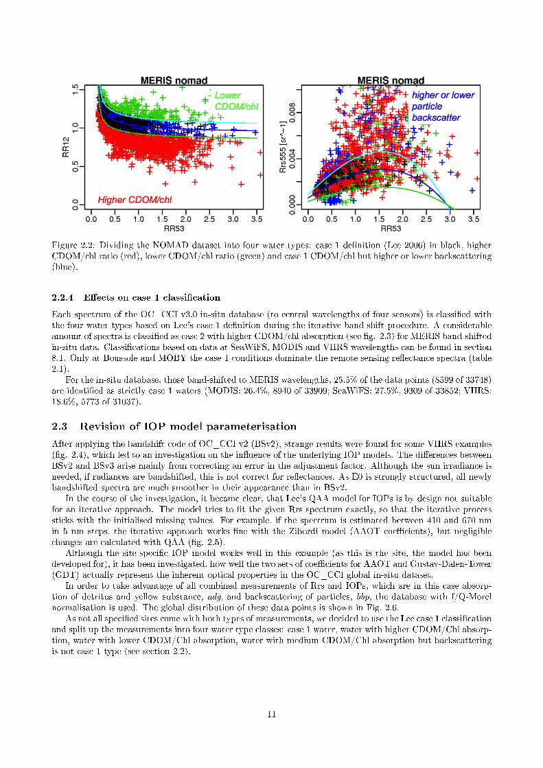
Figure 2.2: Dividing the NOMAD dataset into four water types: case 1 de�nition (Lee 2006) in black, higherCDOM/chl ratio (red), lower CDOM/chl ratio (green) and case 1 CDOM/chl but higher or lower backscattering(blue).

2.2.4 E�ects on case 1 classi�cation

Each spectrum of the OC_CCI v3.0 in-situ database (to central wavelengths of four sensors) is classi�ed withthe four water types based on Lee's case 1 de�nition during the iterative band-shift procedure. A considerableamount of spectra is classi�ed as case 2 with higher CDOM/chl absorption (see �g. 2.3) for MERIS band-shiftedin-situ data. Classi�cations based on data at SeaWiFS, MODIS and VIIRS wavelengths can be found in section8.1. Only at Boussole and MOBY the case 1 conditions dominate the remote sensing re�ectance spectra (table2.1).

For the in-situ database, those band-shifted to MERIS wavelengths, 25.5% of the data points (8599 of 33748)are identi�ed as strictly case 1 waters (MODIS: 26.4%, 8940 of 33909; SeaWiFS: 27.5%, 9309 of 33852; VIIRS:18.6%, 5773 of 31037).

2.3 Revision of IOP model parameterisation

After applying the bandshift code of OC_CCI v2 (BSv2), strange results were found for some VIIRS examples(�g. 2.4), which led to an investigation on the in�uence of the underlying IOP models. The di�erences betweenBSv2 and BSv3 arise mainly from correcting an error in the adjustment factor. Although the sun irradiance isneeded, if radiances are bandshifted, this is not correct for re�ectances. As E0 is strongly structured, all newlybandshifted spectra are much smoother in their appearance than in BSv2.

In the course of the investigation, it became clear, that Lee's QAA model for IOPs is by design not suitablefor an iterative approach. The model tries to �t the given Rrs spectrum exactly, so that the iterative processsticks with the initialised missing values. For example, if the spectrum is estimated between 410 and 670 nmin 5 nm steps, the iterative approach works �ne with the Zibordi model (AAOT coe�cients), but negligiblechanges are calculated with QAA (�g. 2.5).

Although the site-speci�c IOP model works well in this example (as this is the site, the model has beendeveloped for), it has been investigated, how well the two sets of coe�cients for AAOT and Gustav-Dalen-Tower(GDT) actually represent the inherent optical properties in the OC_CCI global in-situ dataset.

In order to take advantage of all combined measurements of Rrs and IOPs, which are in this case absorp-tion of detritus and yellow substance, adg, and backscattering of particles, bbp, the database with f/Q-Morelnormalisation is used. The global distribution of these data points is shown in Fig. 2.6.

As not all speci�ed sites come with both types of measurements, we decided to use the Lee case 1 classi�cationand split up the measurements into four water type classes: case 1 water, water with higher CDOM/Chl absorp-tion, water with lower CDOM/Chl absorption, water with medium CDOM/Chl absorption but backscatteringis not case 1 type (see section 2.2).

11

MERIS

MODIS

SeaWiFS

VIIRS

site

case

1case

2H

case

2L

case

2b

case

1case

2H

case

2L

case

2b

case

1case

2H

case

2L

case

2b

case

1case

2H

case

2L

case

2b

aocAbuAl

Bukhoosh

116

452

015

120

440

023

116

453

014

106

466

011

aocCOVE

SEAPRISM

15

511

027

15

516

022

16

516

021

15

522

016

aocGloria

49

950

0100

79

951

069

59

952

088

50

973

076

aocGustav

DalenTower

107

1348

164

116

1371

033

103

1368

049

88

1387

045

aocHelsinki

Lighthouse

146

1567

154

134

1597

136

134

1593

140

122

1605

140

aocLISCO

38

1015

031

36

1043

05

32

1042

010

25

1052

07

aocLucinda

0281

02

0281

02

0281

02

0281

02

aocMVCO

123

3568

0133

138

3595

091

124

3591

0109

98

3640

086

aocPalgrunden

51

1072

02

49

1076

00

50

1075

00

45

1078

02

aocVenice

551

6191

11994

543

6246

01948

544

6317

11875

537

6511

01689

aocWaveCIS

SiteCSI6

221

1850

0112

238

1868

077

226

1862

095

194

1909

080

boussole

2000

1282

465

72446

754

501

53

2161

1106

476

11

2190

1086

468

10

merm

aid

BioOptEu-

roFleets

025

08

025

08

025

08

026

07

merm

aid

SIM

BADA

166

145

24

46

117

121

36

107

141

137

29

74

144

139

24

74

nomad

1205

1186

231

222

1221

1031

304

288

822

645

172

106

1230

1155

236

223

seabassval

119

68

40

48

101

67

57

50

51

17

17

14

114

70

43

48

moby

3692

72

13587

0257

19

4730

0348

3815

0175

1

Total

8599

21518

765

2866

8940

20982

1156

2831

9309

20980

1044

2519

5773

21900

947

2417

Table2.1:Amountofcase

1andcase

2waterspectrain

OC_CCIv3.0

band-shifteddatabase

(Norm

alisation:fQMorel).

12

0.0

0.5

1.0

1.5

2.0

2.5

3.0

3.5

0.00.51.01.5

ME

RIS

ao

c_G

usta

v_D

ale

n_To

wer

RR

53

RR12

0.0

0.5

1.0

1.5

2.0

2.5

3.0

3.5

0.0000.0040.008

ME

RIS

ao

c_G

usta

v_D

ale

n_To

wer

RR

53

Rrs555 [sr^−1]

0.0

0.5

1.0

1.5

2.0

2.5

3.0

3.5

0.00.51.01.5

ME

RIS

ao

c_H

els

inki_

Lig

hth

ou

se

RR

53

RR12

0.0

0.5

1.0

1.5

2.0

2.5

3.0

3.5

0.0000.0040.008

ME

RIS

ao

c_H

els

inki_

Lig

hth

ou

se

RR

53

Rrs555 [sr^−1]

0.0

0.5

1.0

1.5

2.0

2.5

3.0

3.5

0.00.51.01.5

ME

RIS

ao

c_P

alg

run

den

RR

53

RR12

0.0

0.5

1.0

1.5

2.0

2.5

3.0

3.5

0.0000.0040.008

ME

RIS

ao

c_P

alg

run

den

RR

53

Rrs555 [sr^−1]

0.0

0.5

1.0

1.5

2.0

2.5

3.0

3.5

0.00.51.01.5

ME

RIS

ao

c_V

en

ise

RR

53

RR12

0.0

0.5

1.0

1.5

2.0

2.5

3.0

3.5

0.0000.0040.008

ME

RIS

ao

c_V

en

ise

RR

53

Rrs555 [sr^−1]

0.0

0.5

1.0

1.5

2.0

2.5

3.0

3.5

0.00.51.01.5

ME

RIS

bo

usso

le

RR

53

RR12

0.0

0.5

1.0

1.5

2.0

2.5

3.0

3.5

0.0000.0040.008

ME

RIS

bo

usso

le

RR

53

Rrs555 [sr^−1]

0.0

0.5

1.0

1.5

2.0

2.5

3.0

3.5

0.00.51.01.5

ME

RIS

no

mad

RR

53

RR12

0.0

0.5

1.0

1.5

2.0

2.5

3.0

3.5

0.0000.0040.008

ME

RIS

no

mad

RR

53

Rrs555 [sr^−1]

0.0

0.5

1.0

1.5

2.0

2.5

3.0

3.5

0.00.51.01.5

ME

RIS

seab

ass

RR

53

RR12

0.0

0.5

1.0

1.5

2.0

2.5

3.0

3.5

0.0000.0040.008

ME

RIS

seab

ass

RR

53

Rrs555 [sr^−1]

0.0

0.5

1.0

1.5

2.0

2.5

3.0

3.5

0.00.51.01.5

ME

RIS

mo

by

RR

53

RR12

0.0

0.5

1.0

1.5

2.0

2.5

3.0

3.5

0.0000.0040.008

ME

RIS

mo

by

RR

53

Rrs555 [sr^−1]

Figure

2.3:Classi�cationofOC_CCIv3.0in-situdatabase

band-shiftedto

MERIS

wavelengthsper

site,distinguishingfourtypes

ofwater:case

1de�nition

(Lee

2006)in

black,higher

CDOM/chlratio(red),lower

CDOM/chlratio(green)andcase

1CDOM/chlbuthigher

orlower

backscattering(blue).

13

(a) Bandshift v2 (b) Bandshift v3

Figure 2.4: Example of iterative bandshift on an aoc_AAOT spectrum at VIIRS wavebands. Black circles aremeasurements, red circles are starting points of the iteration process. The line connects measurements andresults of the bandshift. Di�erences arise mainly from new IOP model and from an error in v2, which uses E0in the adjustment, although this is not correct for re�ectances. The jump in the blue is avoided in v3.

(a) Bandshift v3 beta, IOPs Zibordi coe�cients for AAOT (b) Bandshift v3 beta, IOPs QAA

Figure 2.5: Example of iterative bandshift on a aoc_AAOT spectrum at full spectrum with 5nm steps. Blackcircles are measurements, red circles are starting points of the iteration process. (For re�ectances: no E0 in theadjustment.) The QAA IOP model is designed to �t a given Rrs spectrum perfectly, therefore it is not suitablefor the iteration approach.

14

(a) Chlorophyll conc.

(b) adg

(c) bbp

Figure 2.6: Measurements of chlorophyll conc., adg and bbp with remote sensing re�ectances in the OC_CCIin-situ database v3 (Normalisation f/Q Morel). Colours represent the four water classes: case 1 (black), higherCDOM/chl abs. (red), lower CDOM/chl abs. (green), case 1 abs but stronger scattering (blue).

15

a0 a1 a2 a3

case 1 0.3559 -2.0932 0.7760 -2.0278high CDOM/chl 0.1218 2.5334 0.9029 0low CDOM/chl 0.5064 -1.728 -0.5352 1.3864

medium CDOM/chl, high backscatter 0.3352 -2.4827 0 0.6780

Table 2.2: Chlorophyll model. Parameter for four water classes.

Slope b0 b1

case 1 0.0132 -0.5475 -0.4802high CDOM/chl 0.0141 0.0422 -0.7784low CDOM/chl 0.0128 -0.3852 -0.6726

medium CDOM/chl, high backscatter 0.0134 -0.0061 -0.8737

Table 2.3: Parameterisation of adg model.

2.3.1 Chlorophyll concentration

The new chlorophyll models (yellow lines in �g. 2.7) give higher chlorophyll estimates than the AAOT orGDT parameterisation. The AAOT model does not represent the chlorophyll concentration to Rrs ratio of theOC_CCI in-situ data set very well. It is more similar to the all water samples, where the CDOM absorption ishigher compared to a given chlorophyll absorption, than a case 1 model would suggest.

The chlorophyll concentration is modelled with a polynomial function of third degree withR = log10Rrs490/Rrs555

log10 chl = a0 + a1R+ a2R2 + a3R

3 (3)

Only statistically signi�cant coe�cients are taken into account (tab. 2.2). Of course, in a direct comparisonbetween measured and modelled chlorophyll concentration the new model (which is �tted directly to the data)leads to signi�cantly better results than the polynomial model with the AAOT coe�cients, which has beenused before (Fig. 2.8). Especially smaller concentrations have been poorly represented before and heavilyunderestimated in the previous version.

2.3.2 Absorption of total dissolved matter, adg

In the same manner, the relationship between Rrs 490 and 670 nm (R = log10Rrs490/Rrs670) and absorptionof detritus and gelbsto� adg, has been revised (tab. 2.3). It replaces the estimations of ay + adp.

log10 adg412 = b0 + b1R (4)

adg (λ) = adg412 · exp (−Slope · (λ− 412)) (5)

A comparison of modelled adg or adp + ay values against measured values is shown in Fig. 2.9. The modelwith AAOT coe�cients tends to underestimate the absorption of adg.

2.3.3 Backscattering of particles

The backscattering is revised as well.With R = log10 Lwn(490)/Lwn(555) the backscattering is modelled with an exponential decline (see table

2.4):

log10 bbp(510nm) = d0 + d1 ·R

log10 bbp(λ) = log10 bbp(510nm) · (λ/510)−Sbp

The previous model overestimated the measured particle backscattering (Fig. 2.10).

16

Figure 2.7: Chlorophyll models based on the OC_CCI v3.0 in-situ data and four water type classes (based onLee de�nition). Green line represents the Zibordi AAOT model, the blue line the Zibordi GDT model. Theyellow lines are the four models, which are used in the BS v3 for this study.

Sbp d0 d1

case 1 1 -2.3816 -1.3803high CDOM/chl 1 -2.2632 -1.8359low CDOM/chl 1 -2.4386 -1.2018

medium CDOM/chl, high backscatter 1 -2.2011 -2.0701

Table 2.4: Parameterisation of backscattering model.

17

(a) case 1 Lee 2011

(b) higher CDOM/chl absorption

(c) lower CDOM/chl absorption

(d) medium CDOM/chl absorption, but higher scattering

Figure 2.8: Modelled chlorophyll concentration versus in-situ chla_�uor or chla_hplc.18

(a) case 1 (Lee 2006)

(b) Higher CDOM/chl absorption

(c) Lower CDOM/chl absorption

(d) Medium CDOM/chl absorption, but higher backscattering

Figure 2.9: Modelled adg or adp + ay (AAOT) versus in-situ adg. All spectral values are joined.19

(a) case 1 (Lee 2006)

(b) Higher CDOM/chl absorption

(c) Lower CDOM/chl absorption

(d) case 1 CDOM/chl absorption, but higher backscattering

Figure 2.10: Modelled bbp versus in-situ bbp.20

2.4 Band-shifting procedures

The bandshifting procedures need some estimation of IOPs and chlorophyll from the given remote sensingre�ectances. Two di�erent IOP models are implemented: QAA v5 and the parametric models from section 2.3.Three di�erent types of corrections are implemented: two iterative corrections are based on f/Q tables (withcorrections based on one or two nearest measurements to the target), while the third one uses the forward modeof QAA to derive correction factors without iteration.

The iterative approach is robust and works well even with very limited numbers of available measurements.For each satellite sensor the nominal wavelengths of the spectral bands are given as

MERIS = 412, 442, 490, 510, 560, 620, 665, 681, 709, 753, 779, 865, 885 nm,

MODIS = 412, 443, 488, 531, 547, 667, 678, 748, 869 nm,

SeaWifS = 412, 443, 490, 510, 555, 670, 765, 865 nm,

VIIRS = 412, 445, 488, 555, 672 nm.

The models for IOPs and chlorophyll follow the descriptions in section 2.3.

2.4.1 Iterative method employing f/Q

The nominal wavelengths and those needed for IOP estimation are combined and the unique set of wavelengthsis selected and sorted, while wavelengths above 682 nm are discarded. This limit was 678 nm in the earlierBS v2. Each spectrum is considered separately. Measurements at all available wavelengths are taken intoaccount. The combination of nominal wavelengths and those needed for IOP modelling are initialised, either withactual measurements (within ±1nm) or by linear interpolation between measured spectral points. Duplicatesof wavelengths after copying values in the ±1nm range are discarded, only the targeted nominal wavelength iskept. For each target wavelength, the two closest Rrs measurements are identi�ed (λstart1, λstart2). From theinitialised Rrs values the water class and the chlorophyll conc and IOPs are estimated.

The procedure follows Zibordi et al. [2009] to some length, but combines it with an iterative approach andmodelling the Rrs

Rrs (λtarget, λstart) = Rrs (λstart)

fQ0

(λtarget, chl)bb(λtarget)a(λtarget)

fQ0

(λstart, chl)bb(λstart)a(λstart)

(6)

with fQbba in order to allow for larger di�erences between start and target wavelength (communication Mélin).1

All constants (f/Q, and water optical properties) are linearly interpolated towards the exact wavelength of themeasurements.

The chlorophyll concentration is estimated from Rrs at 490 and 555 nm. Estimates for CDOM absorptionay and non-pigmented particles absorption adp, combined in adg and pigmented particle (phytoplankton) ab-sorption aph, particle backscattering bbp are calculated and combined with tabulated water absorption aw andbackscattering bw to total absorption and backscattering at all designated and measured wavelengths.

The number of iterations is restricted to a maximum of 20 initially. As a start wavelength, the two closestmeasured wavelengths to the target are selected. After calculating both estimates at the target wavelength, theyare combined in a weighted (inverse distance) mean. Although di�erences between start and target wavelengthcan be rather large, the procedure converges almost always - an important improvement compared to theprevious version, which su�ered from divergent or alternating behaviour in the estimates.

Rrs (λtarget) = w1Rrs(λstart 1) + w2Rrs(λstart 2)

The convergence limit is de�ned as the mean absolute deviation in Rrs between two iteration steps over theentire spectrum, which should be lower than ε = 10−9 and

1

Nλ

Nλ∑i=1

‖Rrs (λi, n)−Rrs (λi, n+ 1)‖ < ε (7)

1There has been an error in the previous version. Although the water leaving radiance is modelled as Lwn (λ) =

E0 (λ)fQ0

(λ, chl)bb(λ)a(λ)

and therefore includes E0, the remote sensing re�ectance is independent from E0. Rrs(λ) = Lwn (λ) /E0 (λ).

21

(a) Bandshift v3 beta, IOPs Zibordi coe�cients for AAOT (b) Bandshift v3, water class IOPs

Figure 2.11: Example of iterative bandshift on a boussole spectrum at full spectrum with 5nm steps. Blackcircles are measurements, red circles are starting points of the iteration process. The AAOT IOP model coversthe water type at BOUSSOLE not as well as the new model for water class 0 (which corresponds with the Leecase 1 de�nition)

If the series of chlorophyll values is converging but the convergence limit is not reached, the maximumnumber of iterations is raised stepwise by 20 iterations up to a total of 100. The values at the missing designatedwavelengths are replaced by these estimates. If the convergence limit is not met, these values are used as thenew input data for a next step in the iteration. At the moment, the estimated water class stays �xed throughoutthe iteration process.

For quality control purposes the band-shifting can be performed for each site or collection of measurementsseparately, and each Rrs spectrum is plotted with all the iterative steps in between. A second plot shows theestimated chlorophyll concentration per iteration step.

Example The new water class based IOP estimates lead to a bandshift, which gives physically reasonableresults and re�ects the OC_CCI in-situ database (example �g. 2.11).

2.4.2 De�nition of band-shift quality �ags

The outcome of this procedure is assigned a quality �ag per spectrum. The �rst part of the �ag string consistsof a numerical character for each satellite band. The �ag value codes the information about the band-shiftprocedure itself. Only measurement points can be start points. The considered start wavelength is the closestmeasured wavelength to the estimation point.

� Flag value 0: no band-shift necessary for this band, measurement has been within ±1 nm of the designatedwavelength.

� Flag value 1: band-shift has been applied and distance between start and target wavelength has been± 10nm.

� Flag value 2: di�erence between start and target wavelength is larger than ±10 nm.

The second part of the �ag is introduced by an underscore �_�. The �ag value constitutes the state of theconvergence of the error series.

� Flag value 0: the series converges strongly, i.e. the convergence limit is reached in less than 20 iterations.

� Flag value 1: the series converges, but the convergence limit is not reached after 20 iterations.

� Flag value 2: the series diverges.

In addition the number of iterations are kept in the �nal band-shifted dataset.

22

2.4.3 Selection of band-shifted data

In the next step, the band-shifted data is prepared for easy application.

� If the series of estimation diverges, only the original values are kept, while estimations are discarded.

� If the series converges, only estimations made within the ±10 nm interval between start and targetwavelength are kept.

Bandshifted and original data are recombined, discarding all spectra with less than 3 spectral data points.The data points, which do not comply with these criteria, are set to NA - so each remaining data point in

the band-shifted database can be used as they are.

2.5 Ideas for future versions

Further information on the band-shift procedures and their validation can be found in an up-coming technicalnote or publication.

2.5.1 Tested

� Test successive updating of band-shift results, using them as new starting values within the same iteration.This approach leads to divergence often and is therefore discarded.

� As QAA �ts a given Rrs spectrum almost perfectly by design, it is not suitable for the iterative approach.

� Often IOP and Rrs data for sites is not available and therefore it is not feasible to provide site speci�c IOPmodels everywhere. The IOP model is no longer chosen according to sites, as the water characteristicscan vary strongly at a single station over time.

� Instead, it has been decided to use a simple water type classi�cation (Lee case1/case2 classi�cation) basedon Rrs measurements and IOP models have been �tted to these partial datasets.

� Update the water type classi�cation with each iteration, as it might change with the on-going estimationof the spectrum. The water type is provided in the output.

2.5.2 Untested

� Use sensor response functions per band to convolute the spectral constants like extra-atmospheric solarirradiance E0, water absorption and backscattering, and bi-directional correction f/Q.

� Instead of water types based on Lee case 1 de�nition, the optical water type classi�cation of the OC_CCIproject can be applied. If the number of in-situ measurements in each of the 14 classes is su�ciently large,the IOP model could be re�ned.

� The Lee case 1 and derived case 2 de�nitions need to be checked against the water type classi�cation orspectra, which represent known water types. Both �xed factors in the Lee algorithm could be adjusted.In particular, the identi�cation of scattering waters seems rather poor.

23

3 Round Robin 3 Protocol

Band-shifting of in-situ data to wavelegths of satellite sensors, as described in the previous section, is the �rststep towards a match-up database, which combines the in-situ data with satellite data. Now further measurescan be taken.

Firstly, it is necessary to de�ne the sets of quality �ags per AC processor, which allow us to choose valid,high quality satellite products (section 3.1.2). In a second step, the aggregation methodology needs to be de�ned(section 3.2). In the course of the inter-comparison, di�erent subsets of data points are used, which are selectedby using individual and combined �ags (IBQ: Individual Best Quality, CBQ: Common Best Quality) and arerestricted to case-1 waters only (section 2.2).

3.1 Atmospheric Correction processors

For the intercomparison of MERIS based normalised water leaving re�ectances, four atmospheric correctionprocessors have been used.

These are

� MEGS 8.1, the ESA standard processor,

� l2gen version 7.2, the NASA processor,

� c2rcc v0.5 without normalisation, for MODIS and SeaWiFS. c2rcc v0.6 with normalisation and revised�ags for MERIS. Inverse neural network.

� POLYMER version 3.4.

The development of a forward neural network has been discontinued. Its place has been taken by the appropriateinverse neural network. A �fth AC processor, siacs (FUBnn), is still under development.

3.1.1 Notes on l2gen processing

� SeaWiFS/l2gen gives only correct �ags, if the data is processed from L1a to L2. Otherwise the straylightand HILT �ag is wrongly raised in about 90% of all cases.

� MERIS/l2gen uses a parameter �le with input parameter rad_opt set to 1, which ensures the applicationof the MERIS smile correction (similar to MEGS).

� MODIS, SeaWiFS and VIIRS are processed to L1c, so that radiometric corrections are applied correctlyto the data.

3.1.2 AC processor quality �ags

The screening of pixels has been revised in some parts.Additional cloud �ags are available for the four satellite sensors from the Idepix processor, which identi�es

land, cloud, snow/ice and mixed pixels. For further information, please refer to the Idepix ATBD.All atmospheric corrections provide sets of quality �ags, and in the aggregation process the individual �ags

and the information from Idepix are combined.Changes in the AC �ags are made for POLYMER, which discards the threshold at 412 nm, but allows for

case 2 conditions.

� Idepix cloud mask (version 2.2.13, for all ACs): !F_LAND& !F_CLOUD& !F_SNOW_ICE & !F_MIXED_PIXEL

� Polymer: bitmask == 0 & bitmask == 1024

� c2rcc: v0.5 !(AC_NN_IN_ALIEN | AC_NN_IN_OOR ); v0.6 !(Rtosa_OOR | Rtosa_OOS | Rwa_OOR)

� l2gen: !(LAND | CLDICE | SEAICE | HIGLINT | LOWLW | HILT | MAXAERITER | HISOLZEN |HISATZEN | NAVFAIL| ATMWARN | ATMFAIL | STRAYLIGHT)

� MEGS: !(CLOUD | LAND | ICE_HAZE | HIGH_GLINT | PCD_1_13 | PCD_19)

24

3.1.3 System Vicarious Calibration Gains

POLYMER v3.4 (PR05) (version 20150929)

� SeaWiFS: CALIB 1.0062 1.0007 0.9967 0.9921 1.0 1.0 1.0 1.0

� MODIS: CALIB 1.0128 1.0186 1.0 1.0152 1.0154 1.0153 1.0 1.0 1.0076 1.0 1.0 1.0 1.0 1.0

� MERIS: CALIB 0.9921 0.9949 0.9921 0.9950 0.9938 1.0023 0.9985 1.0 1.0 1.0 1.0 1.0 1.0 1.0 1.0

� VIIRS: l2gen gains

3.2 Extraction, Aggregation and Filtering

3.2.1 Automated extraction with CalValus

After uploading the bandshifted in-situ data, the production with di�erent AC processors and extraction ofsatellite data is done automatically on the CalValus system.

The extraction parameters are set to a macro pixel size of three pixels, and a maximum time di�erencebetween in-situ and satellite observation of three hours.

Only the �rst data point of overlapping macro-pixels is considered (overlap �lter) and the macro-pixel hasto be complete (here three by three pixels).

3.2.2 Aggregation and Filtering methodology

The aggregation process can vary quite strongly in terms of �ltering techniques on the macro-pixel and theactual aggregation from the macro-pixel to a single value in the inter-comparison.

The extraction of satellite data consists of the (uneven) N by N pixel, for which the central pixel is closest tothe in-situ location. If for a single satellite scene several in-situ measurements at the same location are available,only the one closest in time is considered. The over�ight and the in-situ measurement have to occur within a±3 hours time di�erence.

A match-up point of good quality is created and selected by the following method:

� To each pixel in the macro-pixel, the de�ned AC �ags are applied and only valid pixels are considered inthe next steps.

� An outlier �lter in form of a standard deviation (σ) �lter is applied to the remaining pixels per wavelengthin the macro-pixel. If the pixels are within µλ − f · σλ ≤ Rrsn (λ) ≤ µλ + f · σλ, with factor f = 1.5 asdefault, they are kept as valid. This �lter is applied to each wavelength independently, as noise can bewavelength dependent.

� If the number of valid pixels remains larger than half of the size of the macro-pixel, Nvalid > N2/2,

� the mean µ and standard deviation σ of the remaining pixels (per wavelength) is calculated and used totest for spatial homogeneity. If σλ/µλ < 0.15, the macro-pixel is considered to be spatially homogeneousand the mean of the remaining valid pixels is a good representative of the entire macro-pixel measurement.

Due to the movement of the water body it seems necessary to account for the time di�erence between in-situmeasurement and satellite over�ight with the averaging of the homogeneous macro-pixel. But it is also possibleto use the central pixel only. In this case, the instrument noise (or processor noise) becomes a larger issue,which can be more easily neglected in an averaging approach.

Even after aggregation further �ltering might be considered, although this is a purely cosmetic step, whichtakes the sensitivity of the statistical parameters on outliers and the demand for gaussian distributed valuesinto account, but is not driven by oceanographic or physical arguments.

3.3 IBQ, CBQ and case 1 de�nition

3.3.1 CBQ cautionary note

Although the CBQ (Common Best Quality) �ags are the combination of all processor �ags and for each processorthe same pixels are chosen, the aggregated data points are not necessarily selected as good match-up points forall processors.

25

� During �ltering, outliers may or may not exist for a certain processor, so that the amount of valid pixelscan decrease below the limit for one processor but not for another due to processor speci�c noise in thedata.

� The homogeneity criterion can lead to a di�erent amount of available good match-up points, which isagain dependent on the noise.

There is no �lter in place, which selects only those aggregated spectral points, which are available for allprocessors.

3.3.2 CBQ and the case 1 selection

In Round Robin 2, the water type selection has been based on the satellite data.In order to avoid di�erences in appointed water types, the classi�cation is based on the in-situ data spectrum

in Round Robin 3. Either during band-shift or by analysing the spectrum, the water type is assigned to thein-situ data and is independent from the AC retrieval.

3.4 Further investigation

� For inhomogeneous case 2 waters, the aggregation procedure could use a single centre pixel instead of themean of the (valid) macro pixel.

26

Figure 4.1: Scoring scheme relating points to the best instance with the highest quality (blue). Numbers arethe appointed scores after normalisation.

4 Statistics and Scoring

4.1 Statistical parameters

Unlike in the �rst round robin where several more statistical parameters have been included in the selectionprocess, their number has been reduced to four now. The remaining parameters are:

� RMSE (abs.)

� Bias (abs.)

� residual error (abs.)

� χ2

The other parameters (relative RMSE, correlation coe�cient, slope and intercept of linear regression, number ofvalid points, the number of spectra with a χ2 lower than the 95% con�dence level) are in some parts redundant.For MERIS seven wavelengths are considered, for MODIS and SeaWiFS six wavelengths are part of the study,for VIIRS �ve. As some wavelengths are very rarely measured in-situ, the χ2 value is based on �ve wavelengthsfor all the sensors.

4.2 Scoring scheme

Most of the statistical properties come with a standard error or 95% con�dence interval. All properties aretransformed to negative oriented values, if necessary. To each property the evaluation scores are assigned bywavelength separately in the following manner (Fig. 4.1):

� The best algorithm is the one with the smallest value in the statistical property and receives 2 points.

� If the value corresponding to another algorithm falls within the con�dence interval of the best, thisalgorithm is not signi�cantly di�erent from the best and receives 2 points as well.

� If the value of another algorithm lies outside the con�dence interval of the best but their con�denceintervals overlap, this algorithm receives 1 point.

� If the con�dence interval of an algorithm does not overlap with the best algorithm, this algorithm receives0 points.

� In order to weigh each wavelength equally the scores will be normalised, so that the sum of all points perwavelength and property over all algorithms equals 1.

All scores S are then summed up per wavelength and statistical property, which gives each of them equal weight.The measure of spectral shape, i.e. the mean χ2 value, receives the same weight as a single waveband. Thescore is therefore multiplied by three (because there are three statistical parameters considered per wavelength),when added up to a total score.

Stotal (Processor) =∑7i=1 SRMSE.abs (λi) + Sres.error.abs (λi) + Sbias (λi) + 3 · Sχ2 (8)

27

In favouring the best algorithm strongly, this scoring system tends to a non-linear behaviour. This approachhas been preferred over one of relative scores, which considers all relationships to �xed limits per statisticalparameters. It would have been necessary to de�ne in absolutes of what is supposed to be a �good result�.The choice would have been highly subjective. Another scoring approach which is applied in the comparisonof in-water algorithms (Brewin et al. [2012]) uses the larger number of algorithms to its bene�t. From overten di�erent retrieval algorithms for water constituents the mean of the statistical value under study and thecon�dence interval are calculated. All algorithms which perform within the con�dence interval get the samescore, while algorithms outside the interval receive a score of zero. With only four algorithms available thisapproach cannot be applied to the atmospheric correction comparison.

28

Figure 5.1: Round Robin software overview. Some software parts are implemented in R (green), others on theCalValus system (dark blue).

5 Round Robin automated tools

5.1 Overview

Several steps of the round robin procedure have been developed and implemented in di�erent software parts(Fig. 5.1).

The user needs to perform the band-shift of the in-situ database and needs to apply an R-Script for thistask.

The band-shifted in-situ database (including columns with latitude, longitude and time information, anda unique numbering of the data points for sorting purposes afterwards) has to be uploaded to the CalValussystem. With the help of the match-up processor, the level 2 products are calculated based on a level 1 satellitedatabase. Although there is a capability for processor dependent �ags and aggregation in place on CalValus,we decided to use the overlap �lter only, which eliminates duplicates in time for a single place and a single day.Only the in-situ measurement closest in time to the over�ight is considered, which can be di�erent for eachsatellite sensor.

The resulting tables with the L2 products are downloaded. It is necessary to change a single character inall POLYMER processed data �les. The POLYMER processor includes a product �R'865�, but the followingprocedures in R are not able to read in the apostrophe and would crash. Using the Python interface, theparameter �les for the aggregation and statistics procedures can be easily set and run.

If changes to the statistics and scoring scheme have been made, it is necessary to upload a new softwarebundle to CalValus as well, which consists of exactly the same procedures as they have been used to analysethe single representation(s). Bootstrapping the statistics and the scores needs the aggregated match-up datato be uploaded to the CalValus system again. The statistical analysis results in an automatically generateddocumentation including scatterplots and tables of statistics and scores. The bootstrapping results need to beplotted with a separate script and are not yet automatically included in the documentation.

29

5.2 Round Robin Aggregation and Statistics Interface

Primarily the Python GUI for the aggregation and the statistical analysis is an interface, which allows the userto write R-script �les with selected parameters (further on �parameter �les�) and invoke the R-scripts for thecalculations.

The following sections give short summaries of the functionality of this analysis tool.

5.2.1 Data Selection (Fig. 5.2)

Sensor Four satellite sensors are implemented at the moment. If the selection is changed, the user shouldalso press the �Initialise� button, which will then change the default settings of processor type, processornames, �ags and variable names to the satellite speci�c default values.

Initialise button Pressing the �Initialise� button will change the default settings of processor types, processornames, �ags and variable names to the selected satellite speci�c default values.

Processor - Extractions The default value �/path/� has to be replaced by the actual path to the appropriateCalValus extraction �le, which contains the not aggregated 3x3 pixel data. The �le can be selected bypressing the button and navigating with the �le manager to the location. If the default value is notchanged, the script assumes, that no data exists.

Processor type Select the processor type (POLYMER, MEGS, ForwardNN, l2gen, FUBnn). After changingthe processor type the Processor name (processor speci�cation), the �ags and the water leaving re�ectancevariable names can be set to the speci�c default values by pressing the �Initialise� button. Default valueswill be set in all processor instances - if you have already made changes to one, they will be lost.

Processor spec Give a unique version or speci�cation number to the processor. The name will be usedthroughout the entire analysis and appear in diagnostic plots. The user should choose a name withoutblanks and dots.

Flags The text �eld holds the �ag expression in R syntax, which will be used to identify valid pixels.

Variables give the names of the products which are aggregated in coming calculations and are therefore partof the validation exercise. The default values are the normalised water leaving re�ectances of the di�erentatmospheric correction processors.

5.2.2 Data sorting (Fig. 5.3)

The extracted datasets can slightly di�er in the order of extracted points. As the aggregated data will becombined in a single �le, so that selecting subsets for the bootstrapping becomes easy, it is necessary, thatthe extractions are in the same order. Sorting can be quite time consuming and it is well advised to includea column of continuous numbering in the band-shifted in-situ dataset, so that the same measurements can beidenti�ed easily.

If the data can be sorted by such an identi�er, the user can set the column name in the text �eld.

5.2.3 Aggregation parameter setup (Fig. 5.4)

The aggregated data is described by the following parameters:

Output folder can be selected from the �le manager. All output �les, which are the combined (and sorted)aggregated match-up data points from all AC processors, are written into this folder.

In-situ Variables holds the names of the columns with the in-situ data in the table. The default names arejust in�uenced by the choice of the satellite sensor. The user has to make sure, that the number of in-situvariables matches the number of satellite products and that the names are given in the appropriate order.The R script does not check, whether names and content are consistent.

Column name In-situ sites

Column name In-situ time

30

Figure 5.2: Round Robin Python GUI Part 1- data selection. Default settings.

Figure 5.3: Round Robin Python GUI Part 2 - Sorting and addition of Idepix �ags setup. Default settings.

31

Column name satellite time

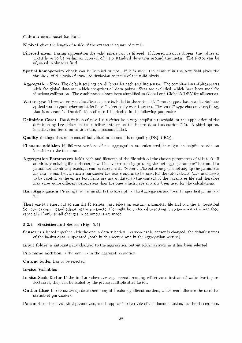
N pixel gives the length of a side of the extracted square of pixels.

Filtered mean During aggregation the valid pixels can be �ltered. If �ltered mean is chosen, the values atpixels have to be within an interval of ±1.5 standard deviation around the mean. The factor can beadjusted in the text �eld.

Spatial homogeneity check can be applied or not. If it is used, the number in the text �eld gives thethreshold of the ratio of standard deviation to mean of the valid pixels.

Aggregation Sites The default settings are di�erent for each satellite sensor. The combinations of sites startswith the global data set, which comprises all data points. Sites are excluded, which have been used forvicarious calibration. The combinations have been simpli�ed to Global and Global-MOBY for all sensors.

Water type Three water type classi�cations are included in the script. �All� water types does not discriminateoptical water types, whereas �strictCase1� selects only case 1 waters. The �case2� type chooses everything,that is not case 1. The de�nition of case 1 is selected in the following parameter

De�nition Case1 The de�nition of case 1 can either be a very simplistic threshold, or the application of thede�nition by Lee either on the satellite data or on the in-situ data (see section 2.2). A third option,identi�cation based on in-situ data, is recommended.

Quality distinguishes selections of individual or common best quality (IBQ, CBQ).

Filename addition If di�erent versions of the aggregation are calculated, it might be helpful to add anidenti�er to the �lenames.

Aggregation Parameters holds path and �lename of the �le with all the chosen parameters of this task. Ifan already existing �le is chosen, it will be overwritten by pressing the �set aggr. parameter� button. If aparameter �le already exists, it can be chosen with �Select�. The entire steps for setting up the parameter�le can be omitted, if such a parameter �le exists and is to be used for the calculations. The user needsto be careful, as the entire text �elds are not updated to the content of the parameter �le and thereforemay show quite di�erent parameters than the ones which have actually been used for the calculations.

Run Aggregation Pressing this button starts the R script for the Aggregation and uses the speci�ed parameter�le.

There exists a short cut to run the R scripts: just select an existing parameter �le and run the aggregation!Sometimes copying and adjusting the parameter �le might be preferred to setting it up anew with the interface,especially if only small changes in parameters are made.

5.2.4 Statistics and Scores (Fig. 5.5)

Sensor is selected together with the one in data selection. As soon as the sensor is changed, the default namesof the in-situ data is up-dated (both in this section and in the aggregation section).

Input folder is automatically changed to the aggregation output folder as soon as it has been selected.

File name addition is the same as in the aggregation section.

Output folder has to be selected.

In-situ Variables

In-situ Scale factor If the in-situ values are e.g. remote sensing re�ectances instead of water leaving re-�ectances, they can be scaled by the giving multiplicative factor.

Outlier �lter In the match-up data there may still exist signi�cant outliers, which can in�uence the sensitivestatistical parameters.

Parameters The statistical parameters, which appear in the table of the documentation, can be chosen here.

32

Figure 5.4: Round Robin Python GUI Part 3 - aggregation parameter setup. Default settings.

Score Parameters These statistical parameters are used for the scoring. (The script does not check whetherthe statistical parameters have been calculated. The user has to take care that the Score Parameters area subset of the statistical parameters.)

Common Scale Site The scatterplots use a common scale per wavelength. The given site chooses the �le onwhich the common scale will be based.

Aggregation Sites are the same as in the aggregation parameters.

Water Type is the same as in the aggregation parameters.

Quality is the same as in the aggregation parameters.

Scatterplots may or may not be created.

Spectral Statistic Plots may or may not be created.

Score Type can either be �AC�, which corresponds to the method described above (see 4.2), or it can be�multiple�.

Parameter File needs to be selected or created by choosing a path and �lename and then use the �SetStatistics� button. This action will write a text �le including all the information speci�ed in the StatisticsParameter Setup section. Existing �les will be overwritten without warning. As a shortcut it is possibleto select an existing parameter �le and calculate the statistics. Again, choosing an existing parameter �lewill not change the entries in text �elds or selections!

Calculate Statistics Pressing this button will run the statistics script with the given parameter �le (not withinput from the interface itself). If changes in the interface text �elds are made, a new parameter �le hasto be written.

Quit the python program.

33

Figure 5.5: Round Robin Python GUI Part 4- statistics parameter setup. Default settings.

34

6 Round Robin Results - Summary and Discussion

6.1 Match-up extraction with the CalValus System

In a �rst step, the band-shifted in-situ database is uploaded to the CalValus system. With the help of the match-up tool, the corresponding satellite data is identi�ed and processed from level 1 to level 2. All parameters aregiven in section 6.2.

It is imperative for the SeaWifS processing with l2gen to calculate Level 2 products directly from level1a(NASA standard procedure). Otherwise you have to consider that a two-step approach from level 1a to level1b to level 2 might lead to applying the vicarious calibration gains twice!

6.2 Set-up summary

In-situ database: OC_CCI v3.0 (section 1), normalisation following Park and Ruddick mostly, and f/Q Morelfor case 1 observations in NOMAD dataset.

Band-shift: band-shifted iteratively (water type based IOPs, modelled with two closest wavelengths, weightedwith inverse distance), ∆λ < 10nm (only closest wavelength), convergence limit ε = 10−9 (section2)

Match-up protocol: ±3h in-situ measurement and over�ight, extract of full 3x3 pixels, centre closest to in-situposition, no overlap with other extractions.

Filtered mean: µλ − f · σλ ≤ Rrsn (λ) ≤ µλ + f · σλ, with f = 1.5

Homogeneity criterion: σλ/µλ < 0.15 and Nvalid > N2/2, with N = 3

Flag de�nition: see 3.1.2. Idepix cloud mask v2.2.13 is added to each processor.

Outlier �lter: after aggregation is NOT applied.

Case 1 de�nition: Lee and Hu [2006]. (section 2.2) Selection is based on the in-situ data.

Case 2 de�nition: case 2 waters are de�ned as not being case 1 waters. (section 2.2)

Quality: Individual best (IBQ) and common best (CBQ)

Data selection: Sites which are used for vicarious calibration can be excluded from the in-situ database.

� Global: all sites, entire OC_CCI in-situ database

� Global-MOBY: all sites, but without measurements from MOBY.

Statistics and Scores: (section 4.1 and 4.2)

� RMSE

� Bias

� residual error

� χ2

6.3 Results of statistics and scores

6.3.1 MERIS

Statistics The statistics for IBQ Global with all match-up data or restricted to case 1 data are nearly thesame (�gure 6.2a and �gure 6.2b, left). Reducing the global dataset by the MOBY data raises the RMSEbetween 510 and 620nm. Throughout the entire spectrum POLYMER has the lowest RMSE and residual error.In the blue, the RMSE of c2rcc results decreases. The RMSE of all processors changes with the reduction ofthe data, which indicates that the quality of retrieved data in more complex waters is slightly reduced.

The overall bias is quite similar for all processors for the green to red bands, but in the blue POLYMER hasa positive bias opposite to the negative bias in MEGS, l2gen and c2rcc. The absolute value of bias is similar

35

for all these three processors in the global dataset, the bias of POLYMER in the blue is smaller. If MOBY isexcluded from the data, the biases of POLYMER, MEGS and l2gen increases in the blue, whereas the bias ofc2rcc decreases. The bias of l2gen and MEGS also increases signi�cantly at 620nm.

If the in-situ database is restricted to the case 2 waters, the bias is reduced signi�cantly for c2rcc in theblue, while all other processors retrieve data with larger biases. The RMSE for MEGS results increases in theblue, but the strong error at 620nm for l2gen and MEGS gets reduced (�gure 6.1c).

Although the general shapes of the spectral errors based on CBQ data remains the same compared to IBQ,the di�erences between processors become less pronounced (�gure 6.2). POLYMER outperforms the otherprocessors clearly over the entire spectrum with respect to bias and RMSE for Global, Global-MOBY, for thecombination of water types and case 1 waters (�gure 6.2b, �gure 6.2a).

For case 2 waters, products of c2rcc have the smallest bias, but the RMSE is comparable for all processors,except in the blue. c2rcc performs better here.

Scores The scores are based on the three statistical parameters RMSE, bias and residual error, which hasbeen discussed in the previous section. In addition the χ2 value of the spectra is evaluated as well.

For IBQ and CBQ with combined water types or the case 1 selection and in- or excluding MOBY data,POLYMER clearly performs best (�gure 6.3).

In the CBQ/case 2 selection performances over the spectrum are more similar, which leads to the overlappingof the score distributions. The c2rcc results are slightly better. For the IBQ/case 2 data, all processors (exceptfor MEGS) give a similar quality in the results.

At this stage, the case 2 capabilities of some processors are still under development. With the quite diversebehaviour of comparisons at di�erent sites (in the study of system vicarious calibration), it has been decided tobase any algorithm selection on the case 1 water selection.

Therefore, POLYMER is the preferred choice for the MERIS processing.

36

(a) All water types.

(b) Case 1.

(c) Case 2.

Figure 6.1: Spectral statistics IBQ. MERIS

37

(a) All water types.

(b) Case 1.

(c) Case 2.

Figure 6.2: Spectral statistics CBQ. MERIS

38

(a)Global

(b)Global-MOBY

Figure

6.3:BootstrappingMERIS.Colours

referto

POLYMER(blue),MEGS(green),l2gen

(red)andc2rcc(grey).

39

6.3.2 MODIS

Statistics Based on the IBQ/all selection, RMSE of c2rcc results is always the largest. RMSE for l2gen andPOLYMER are very similar. Di�erences can be seen in the spectral biases. While c2rcc has the largest bias inthe blue, the bias is nearly zero from 488nm onwards. l2gen has a quite constant, but overall the largest biasover the entire spectrum. (�gure 6.4a). If MOBY data is excluded, c2rcc performs better at 412nm in termsof RMSE. At 531nm RMSE raises for POLYMER and l2gen, which remain comparable. The bias of c2rcc getslower at 412 but higher between 488 and 547nm. At 531nm all absolute values of biases increase.

For the IBQ/case 1 selection (�gure 6.4b), RMSE drop to lower values for all processors, except for anincrease of c2rcc results at 412nm. l2gen and POLYMER are quite similar in RMSE over the entire spectrum,with a slight advantage for POLYMER. The absolute spectral bias of POLYMER is the lowest, while the biasof c2rcc is comparable to l2gen except for a large deviation at 412nm. If MOBY data is removed, l2gen andPOLYMER are very similar in RMSE, but c2rcc and POLYMER share the lowest spectral bias (except at412nm).

For case 2 waters, the results are very similar to the global dataset without MOBY (�gure 6.4c).All CBQ/all and CBQ/case 1 selections (�gure 6.5b and �gure 6.5a) the spectral RMSE of POLYMER is

the lowest (with small exceptions at 412nm). The bias of POLYMER is the lowest especially in case 1 watersexcluding MOBY data. In that case the absolute bias of c2rcc increases strongly and the l2gen bias slightly.

Again, case 2 results are similar to those, which are based on the global dataset excluding MOBY data(�gure 6.5c).

Scores For the IBQ/all selection the scores are similar for l2gen and POLYMER, favouring l2gen (�gure 6.6).With the application of the CBQ selection, the order changes to highest scores for POLYMER in all watertypes. The in�uence of the common quality �ags on the results is particularly strong in all datasets whichinclude measurements from case 2 waters.

If data from MOBY is removed, the order in the scores stays the same. For CBQ the scores for l2gen andc2rcc are almost identical.

The algorithm selection is mainly based on the summary of statistics for case 1 waters.Whereas the recommendation in RR2 has been to apply l2gen with MODIS data, here in RR3 POLYMER

is chosen for the processing.

40

(a) All water types.

(b) Case 1.

(c) Case 2.

Figure 6.4: Spectral statistics IBQ. MODIS

41

(a) All water types.

(b) Case 1.

(c) Case 2.

Figure 6.5: Spectral statistics CBQ. MODIS

42

(a)Global

(b)Global-MOBY

Figure

6.6:BootstrappingthescoresofMODIS

match-upstatistics.

Colours

referto

POLYMER(green),l2gen

(red)andc2rcc(grey)

43

6.3.3 SeaWiFS

Statistics The spectral RMSE is smoothest for all AC processors in the IBQ/case 1 selection (�gure 6.7, inparticular �gure 6.7b). Results of POLYMER and l2gen show very similar RMSE in case 1 conditions, but assoon as case 2 waters are included RMSE increases for POLYMER at 412 and 555nm. l2gen has a remarkablylow spectral bias for all data selections which include case 1 water samples. In any case, c2rcc is outperformedin RMSE and bias by the other processors. Biases in case 1 waters remain stable for l2gen and POLYMER ifMOBY data is excluded, but for c2rcc the bias at 555 and 670nm increases.

The spectral pattern of the statistical values based on the case 2 subset is similar to the subset of all watertypes without MOBY data (see �gure 6.7c and �gure 6.7a, right). Compared to case 1 conditions, the RMSEis higher at 490 and 555nm for all processors. The overall bias increases compared to case 1 waters.

Selecting the data with CBQ �ags does not change these �ndings (�gure 6.8).

Scores The scores re�ect the poorer performance of c2rcc compared to the other AC processors correctly(�gure 6.9). In concordance with the analysis of the spectral RMSE and bias, l2gen is clearly the best algorithmfor all data sets, which include case 2 waters. If the study is restricted to case 1 conditions, POLYMER andl2gen perform quite similar. The scores are even in favour of POLYMER, if MOBY data is included in thestudy. Since RR2, the system vicarious calibration for POLYMER/SeaWiFS has been well established. If thealgorithm selection is based on the case 1 selection, one would be free to chose between l2gen and POLYMER.Currently, l2gen is chosen as it is the selected algorithm for VIIRS, which leads to equal distribution of processorsbetween the four satellite sensors. Having two POLYMER products (MERIS and MODIS) and two l2genproducts (SeaWiFS, VIIRS) might lead to better consistency within the merged product, instead of usingPOLYMER/SeaWiFS and adding a di�erent processing only at the end of the time series.

44

(a) All water types.

(b) Case 1.

(c) Case 2.

Figure 6.7: Spectral statistics IBQ. SeaWiFS

45

(a) All water types.

(b) Case 1.

(c) Case 2.

Figure 6.8: Spectral statistics CBQ. SeaWiFS

46

(a)Global

(b)Global-MOBY

Figure

6.9:BootstrappingthescoresofSeaWiFSmatch-upstatistics.

Colours

referto

POLYMER(green),l2gen

(red)andc2rcc(grey)

47

7 Round Robin on VIIRS. Preliminary results.

�Like MODIS, the Visible Infrared Imaging Radiometer Suite (VIIRS) is a multi-disciplinary sensor providingdata for the ocean, land, aerosol, and cloud research and operational users. VIIRS spectral coverage will allowfor data products similar to those from SeaWiFS as well as SST, a standard MODIS product. SST is anEssential Climate Variable (ECV) and, through validation with instruments traceable to NIST standards, is aClimate Data Record. Also, as with SeaWiFS and MODIS, the VIIRS scan and orbit geometries will provideglobal coverage every two days.

The VIIRS design incorporates a SeaWiFS-like rotating telescope assembly which protects the optical com-ponents from on-orbit contamination. This will result in greater on-orbit stability than other designs. VIIRSalso has a solar di�user assembly with a stability monitor similar to MODIS for tracking on-orbit performancein visible wavelengths, and a MODIS-like black body calibration target for the infrared bands.

A two-day coverage is a general requirement for ocean ecology and carbon research because microscopicmarine plant (phytoplankton) concentrations are highly variable, particularly in coastal zones. The VIIRS750 m resolution across the entire scan will provide twice the coverage of MODIS and SeaWiFS, which is asubstantial improvement for coastal and estuarine studies in particular. VIIRS also has shortwave infraredbands that can be used for turbid water aerosol corrections.�2

7.1 Datasets for match-up comparisons

7.1.1 OC_CCI in-situ data version 3.0

As NPP has been launched in October 2011, the amount of possible match-ups with in-situ measurements islimited. The previous intercomparison work has shown that the results can be strongly in�uenced by the dataselection and especially investigations in di�erent water types might become unreliable.

In Round Robin 3 (November 2015) 915 match-ups for VIIRS/l2gen have been extracted, which is a rea-sonable number to start analysis even with di�erentiating of the water types.

There are about 1200 POLYMER extracts (IBQ) available, about 900 spectra are classi�ed as case 2 and300 as case 1.

7.1.2 Comparison with MODIS-A data

In order to create a larger match-up data base, the VIIRS Rrs data is also compared with MODIS-Aqua.For the time range of January 2012 to December 2013 the granules of MODIS and VIIRS are selected, which

ful�l the following criteria:

� maximum distance between nadir lines of satellite overpass is 250 km, the time di�erence should be lessthan 15 min and the observed location has between ±60° latitude.

� MODIS 3x3 macro-pixel have to ful�l the criteria of a good match-up point (see ??).

� l2gen �ags: !ATMFAIL !LAND !PRODWARN !HIGLINT !HILT !HISATZEN !COASTZ !STRAYLIGHT!CLDICE !COCCOLITH !HISOLZEN !LOWLW !CHLFAIL !NAVWARN !MAXAERITER !MODGLINT!CHLWARN !ATMWARN !SEAICE !NAVFAIL !FILTER !PRODFAIL

The amount of possible match-ups depends on the spatial and temporal distance (�gure 7.1). As both satelliteshave very close orbits there is a distinct pattern occurring. The colour of the points is de�ned by the date ofthe overpass, ranging from blue in 2012 to magenta at the end of 2013. The points locations correspond to thenadir position of the �rst line of a scene, if this scene includes points, which ful�l the match-up criteria. The�rst nadir pixel does not have to ful�l these criteria itself.

Starting from this selections of scenes, macro-pixels are chosen from a 10km grid. There are three datasetsavailable, which are positioned within a 300 km radius around Boussole (med), within a 250km radius aroundMOBY, or selected from the world wide data set by taking 1 macro-pixel out of 200 (�gure 7.2).

The MODIS data is bandshifted to VIIRS wavelengths with the water type based IOP models and usingonly the closest wavelength (see section �2).

Although this �virtual in-situ match-up� data has been prepared, the extractions have not been processed.

2Introduction from: http://npp.gsfc.nasa.gov/viirs.html

48

(a) Max. distance 250 km, temporal distance 15 min

(b) Max. distance 100 km, temporal distance 15 min

(c) Max. distance 100 km, temporal distance 5 min

Figure 7.1: Overview of global match-up data of VIIRS and MODIS Aqua within di�erent maximum di�erencesin space and time of the nadir observation. Point positions are the �rst line nadir position, if match-ups whichsatisfy the de�nition are found within the entire scene. Colours change with time from blue (January 2012) tomagenta (December 2013).

49

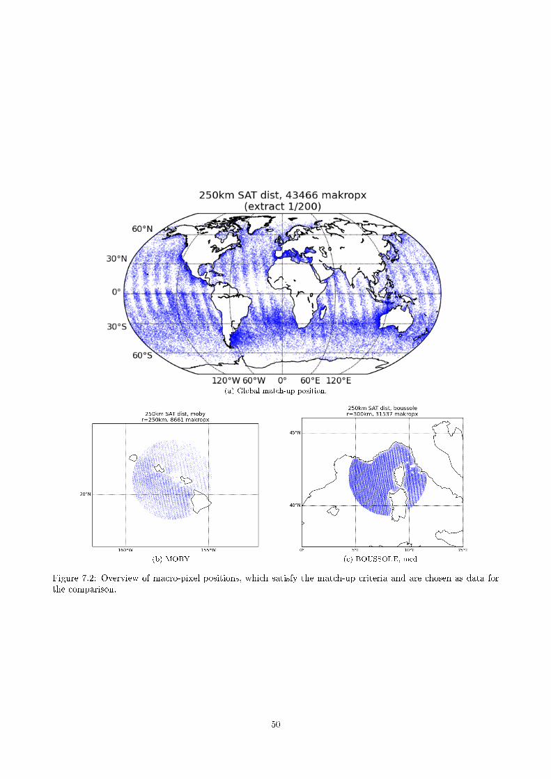
(a) Global match-up position.

(b) MOBY (c) BOUSSOLE, med

Figure 7.2: Overview of macro-pixel positions, which satisfy the match-up criteria and are chosen as data forthe comparison.

50

7.2 Processing VIIRS

At the time of the Round Robin 3 (November 2015), the system vicarious calibration of VIIRS/POLYMER isstill under investigation. The POLYMER processing uses the established l2gen SVC gains instead. Two di�erentversions of the POLYMER processor are tested: the �rst one is based on radiometric models from Morel &Maritorena (polMM01), while the second one employs Park & Ruddick models (PR05). The POLYMERprocessing starts from L1c data, which needs to be processed from L1a.

An IDEPIX cloud mask has not been available yet, but it is in preparation.

Note Starting from L1c introduces an error in the time stamp of the satellite pixel of +1 hour. Therefore inthe time range of ±3hours not all extracts have been found for the POLYMER/VIIRS processing. This leadsto a smaller amount of spectra in the selection of �common best quality� data, as were actually present in theOC_CCIv3.0 dataset. If the l2gen extracts are analysed on their own, 915 match-ups are found. By sortingand combining the data with the POLYMER extracts, only 347 match-ups of l2gen remain. It can be expected,that by correcting this time error, the amount of CBQ spectra would (at least) double.

7.3 VIIRS AC intercomparison

Statistics If the dataset comprises all water types and all sites (IBQ all Global, �gure 7.3a), l2gen has thelowest spectral RMSE followed by polMM01 and polPR05. On the other hand, considering the bias polPR05and l2gen give the best results, while polMM01 has larger biases. If MOBY is excluded, the RMSE of l2genproducts is almost stable, but it raises for the POLYMER spectra (except at 412nm, which shows lower RMSE).The spectral bias of l2gen remains the almost the same, absolute values increase slightly. The bias at 412 nmincreases strongly for the POLYMER processors.

In case 1 waters (Global, IBQ, �gure 7.3b) l2gen has still the lowest RMSE, but the RMSE of polPR05 isquite similar from 486 to 671 nm. In the blue, both POLYMER processors show larger RMSE and also biases.The bias of l2gen is spectrally �at and very close to zero. If MOBY is excluded, the RMSE of polPR05 at443nm increases strongly, whereas values for l2gen remain stable. Still polPR05 and l2gen show very similarRMSE from 486nm onwards. The bias of polMM01 is here spectrally �at and close to zero, while polPR05 andl2gen show increasing (absolute) bias towards the blue.

In case 2 waters (IBQ, �gure 7.3c) l2gen has the lowest spectral RMSE and the lowest absolute bias. AlthoughRMSE of polPR05 is higher than of polMM01, the absolute bias of polPR05 is lower and closer to l2gen.

Changing the �agging of data to the common set of �ags has a rather large in�uence on the statistics.The di�erences between the three AC processors becomes much smaller (CBQ, all global, �gure 7.4a). But forthe blue, the RMSE of polPR05 is the lowest. The bias of polPR05 and l2gen products is very similar, quitesmall and spectrally �at, whereas the products of polMM01 show larger biases at 412 and 551nm. If MOBY isexcluded, the biases of the POLYMER processor change quite strongly in the blue. The spectral bias of l2genproducts increases slightly over the entire spectrum.

As before, in case 1 waters, the spectral RMSE gets smoother (�gure 7.4b). The POLYMER processorshave the higher RMSE errors in the blue, but if MOBY data is excluded the error drops below the l2gen error,which remains quite stable. There is almost no di�erence in RMSE between the three processors from 486nmonwards. The bias of l2gen products is quite small and spectrally �at, whereas the POLYMER processors havesimilar larger biases in the blue. If the data from MOBY is excluded, the biases of polPR05 are the lowest.

In case 2 waters, the spectral RMSE of polPR05 is the lowest (but for 443nm). The spectral bias of l2genis closest to zero.

Scores In the IBQ selections, l2gen receives always the highest scores (�gure 7.5). It has to be pointed out,that these statistics are based on about 340 spectra in contrast to 1200 spectra for the POLYMER processors.

In the majority of cases, polPR05 performs better than polMM01, especially if case 2 water samples are partof the in-situ data. The strong in�uence of the common set of �ags is also re�ected in the scores.

The results are still inconclusive. In an up-coming processing, VIIRS data is processed with l2gen.

51

(a) All water types.

(b) Case 1.

(c) Case 2.

Figure 7.3: Spectral statistics IBQ. VIIRS

52

(a) All water types.

(b) Case 1.

(c) Case 2.

Figure 7.4: Spectral statistics CBQ. VIIRS

53

(a)Global

(b)Global-MOBY

Figure

7.5:BootstrappingthescoresofVIIRSmatch-upstatistics.

Colours

referto

l2gen

(grey),POLYMER

basedonaMorel-Maritorenamodel

(red)

andPOLYMERbasedonPark

&Ruddickmodel(green)

54

8 Illustration appendix

8.1 Water types based on band-shifted in-situ data

55

0.0

0.5

1.0

1.5

2.0

2.5

3.0

3.5

0.00.51.01.5

MO

DIS

ao

c_G

usta

v_D

ale

n_To

wer

RR

53

RR12

0.0

0.5

1.0

1.5

2.0

2.5

3.0

3.5

0.0000.0040.008

MO

DIS

ao

c_G

usta

v_D

ale

n_To

wer

RR

53

Rrs555 [sr^−1]

0.0

0.5

1.0

1.5

2.0

2.5

3.0

3.5

0.00.51.01.5

MO

DIS

ao

c_H

els

inki_

Lig

hth

ou

se

RR

53

RR12

0.0

0.5

1.0

1.5

2.0

2.5

3.0

3.5

0.0000.0040.008

MO

DIS

ao

c_H

els

inki_

Lig

hth

ou

se

RR

53

Rrs555 [sr^−1]

0.0

0.5

1.0

1.5

2.0

2.5

3.0

3.5

0.00.51.01.5

MO

DIS

ao

c_P

alg

run

den

RR

53

RR12

0.0

0.5

1.0

1.5

2.0

2.5

3.0

3.5

0.0000.0040.008

MO

DIS

ao

c_P

alg

run

den

RR

53

Rrs555 [sr^−1]

0.0

0.5

1.0

1.5

2.0

2.5

3.0

3.5

0.00.51.01.5

MO

DIS

ao

c_V

en

ise

RR

53

RR12

0.0

0.5

1.0

1.5

2.0

2.5

3.0

3.5

0.0000.0040.008

MO

DIS

ao

c_V

en

ise

RR

53

Rrs555 [sr^−1]

0.0

0.5

1.0

1.5

2.0

2.5

3.0

3.5

0.00.51.01.5

MO

DIS

bo

usso

le

RR

53

RR12

0.0

0.5

1.0

1.5

2.0

2.5

3.0

3.5

0.0000.0040.008

MO

DIS

bo

usso

le

RR

53

Rrs555 [sr^−1]

0.0

0.5

1.0

1.5

2.0

2.5

3.0

3.5

0.00.51.01.5

MO

DIS

no

mad

RR

53

RR12

0.0

0.5

1.0

1.5

2.0

2.5

3.0

3.5

0.0000.0040.008

MO

DIS

no

mad

RR

53

Rrs555 [sr^−1]

0.0

0.5

1.0

1.5

2.0

2.5

3.0

3.5

0.00.51.01.5

MO

DIS

seab

ass

RR

53

RR12

0.0

0.5

1.0

1.5

2.0

2.5

3.0

3.5

0.0000.0040.008

MO

DIS

seab

ass

RR

53

Rrs555 [sr^−1]

0.0

0.5

1.0

1.5

2.0

2.5

3.0

3.5

0.00.51.01.5

MO

DIS

mo

by

RR

53

RR12

0.0

0.5

1.0

1.5

2.0

2.5

3.0

3.5

0.0000.0040.008

MO

DIS

mo

by

RR

53

Rrs555 [sr^−1]

Figure8.1:Classi�cationofOC_CCIv3.0in-situdatabase

band-shiftedto

MODIS

wavelengthspersite,distinguishingfourtypes

ofwater:case

1de�nition

(Lee

2006)in

black,higher

CDOM/chlratio(red),lower

CDOM/chlratio(green)andcase

1CDOM/chlbuthigher

orlower

backscattering(blue).

56

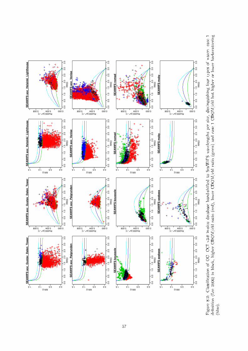
0.0

0.5

1.0

1.5

2.0

2.5

3.0

3.5

0.00.51.01.5

SE

AW

IFS

ao

c_G

usta

v_D

ale

n_To

wer

RR

53

RR12

0.0

0.5

1.0

1.5

2.0

2.5

3.0

3.5

0.0000.0040.008

SE

AW

IFS

ao

c_G

usta

v_D

ale

n_To

wer

RR

53

Rrs555 [sr^−1]

0.0

0.5

1.0

1.5

2.0

2.5

3.0

3.5

0.00.51.01.5

SE

AW

IFS

ao

c_H

els

inki_

Lig

hth

ou

se

RR

53

RR12

0.0

0.5

1.0

1.5

2.0

2.5

3.0

3.5

0.0000.0040.008

SE

AW

IFS

ao

c_H

els

inki_

Lig

hth

ou

se

RR

53

Rrs555 [sr^−1]

0.0

0.5

1.0

1.5

2.0

2.5

3.0

3.5

0.00.51.01.5

SE

AW

IFS

ao

c_P

alg

run

den

RR

53

RR12

0.0

0.5

1.0

1.5

2.0

2.5

3.0

3.5

0.0000.0040.008

SE

AW

IFS

ao

c_P

alg

run

den

RR

53

Rrs555 [sr^−1]

0.0

0.5

1.0

1.5

2.0

2.5

3.0

3.5

0.00.51.01.5

SE

AW

IFS

ao

c_V

en

ise

RR

53

RR12

0.0

0.5

1.0

1.5

2.0

2.5

3.0

3.5

0.0000.0040.008

SE

AW

IFS

ao

c_V

en

ise

RR

53

Rrs555 [sr^−1]

0.0

0.5

1.0

1.5

2.0

2.5

3.0

3.5

0.00.51.01.5

SE

AW

IFS

bo

usso

le

RR

53

RR12

0.0

0.5

1.0

1.5

2.0

2.5

3.0

3.5

0.0000.0040.008

SE

AW

IFS

bo

usso

le

RR

53

Rrs555 [sr^−1]

0.0

0.5

1.0

1.5

2.0

2.5

3.0

3.5

0.00.51.01.5

SE

AW

IFS

no

mad

RR

53

RR12

0.0

0.5

1.0

1.5

2.0

2.5

3.0

3.5

0.0000.0040.008

SE

AW

IFS

no

mad

RR

53

Rrs555 [sr^−1]

0.0

0.5

1.0

1.5

2.0

2.5

3.0

3.5

0.00.51.01.5

SE

AW

IFS

seab

ass

RR

53

RR12

0.0

0.5

1.0

1.5

2.0

2.5

3.0

3.5

0.0000.0040.008

SE

AW

IFS

seab

ass

RR

53

Rrs555 [sr^−1]

0.0

0.5

1.0

1.5

2.0

2.5

3.0

3.5

0.00.51.01.5

SE

AW

IFS

mo

by

RR

53

RR12

0.0

0.5

1.0

1.5

2.0

2.5

3.0

3.5

0.0000.0040.008

SE

AW

IFS

mo

by

RR

53

Rrs555 [sr^−1]

Figure

8.2:Classi�cation

ofOC_CCIv3.0

in-situdatabase

band-shiftedto

SeaWiFSwavelengthsper

site,distinguishingfourtypes

ofwater:

case

1de�nition(Lee

2006)in

black,higher

CDOM/chlratio(red),lower

CDOM/chlratio(green)andcase

1CDOM/chlbuthigher

orlower

backscattering

(blue).

57

0.0

0.5

1.0

1.5

2.0

2.5

3.0

3.5

0.00.51.01.5

VIIR

S a

oc_G

usta

v_D

ale

n_To

wer

RR

53

RR12

0.0

0.5

1.0

1.5

2.0

2.5

3.0

3.5

0.0000.0040.008

VIIR

S a

oc_G

usta

v_D

ale

n_To

wer

RR

53

Rrs555 [sr^−1]

0.0

0.5

1.0

1.5

2.0

2.5

3.0

3.5

0.00.51.01.5

VIIR

S a

oc_H

els

inki_

Lig

hth

ou

se

RR

53

RR12

0.0

0.5

1.0

1.5

2.0

2.5

3.0

3.5

0.0000.0040.008

VIIR

S a

oc_H

els

inki_

Lig

hth

ou

se

RR

53

Rrs555 [sr^−1]

0.0

0.5

1.0

1.5

2.0

2.5

3.0

3.5

0.00.51.01.5

VIIR

S a

oc_P

alg

run

den

RR

53

RR12

0.0

0.5

1.0

1.5

2.0

2.5

3.0

3.5

0.0000.0040.008

VIIR

S a

oc_P

alg

run

den

RR

53

Rrs555 [sr^−1]

0.0

0.5

1.0

1.5

2.0

2.5

3.0

3.5

0.00.51.01.5

VIIR

S a

oc_V

en

ise

RR

53

RR12

0.0

0.5

1.0

1.5

2.0

2.5

3.0

3.5

0.0000.0040.008

VIIR

S a

oc_V

en

ise

RR

53

Rrs555 [sr^−1]

0.0

0.5

1.0

1.5

2.0

2.5

3.0

3.5

0.00.51.01.5

VIIR

S b

ou

sso

le

RR

53

RR12

0.0

0.5

1.0

1.5

2.0

2.5

3.0

3.5

0.0000.0040.008

VIIR

S b

ou

sso

le

RR

53

Rrs555 [sr^−1]

0.0

0.5

1.0

1.5

2.0

2.5

3.0

3.5

0.00.51.01.5

VIIR

S n

om

ad

RR

53

RR12

0.0

0.5

1.0

1.5

2.0

2.5

3.0

3.5

0.0000.0040.008

VIIR

S n

om

ad

RR

53

Rrs555 [sr^−1]

0.0

0.5

1.0

1.5

2.0

2.5

3.0

3.5

0.00.51.01.5

VIIR

S s

eab

ass

RR

53

RR12

0.0

0.5

1.0

1.5

2.0

2.5

3.0

3.5

0.0000.0040.008

VIIR

S s

eab

ass

RR

53

Rrs555 [sr^−1]

0.0

0.5

1.0

1.5

2.0

2.5

3.0

3.5

0.00.51.01.5

VIIR

S m

ob

y

RR

53

RR12

0.0

0.5

1.0

1.5

2.0

2.5

3.0

3.5

0.0000.0040.008

VIIR

S m

ob

y

RR

53

Rrs555 [sr^−1]

Figure

8.3:Classi�cationofOC_CCIv3.0in-situdatabase

band-shiftedto

VIIRSwavelengthsper

site,distinguishingfourtypes

ofwater:case

1de�nition

(Lee

2006)in

black,higher

CDOM/chlratio(red),lower

CDOM/chlratio(green)andcase

1CDOM/chlbuthigher

orlower

backscattering(blue).

58

References

James Aiken, Gerald Moore, Charles C. Trees, Stanford B Hooker, and Dennis K. Clark. The seawifs czcs-typepigment algorithm. Technical Report Vol. 29, NASA Technical Memorandum 104566, 1995.

R.J.W. Brewin, S. Sathyendranath, D. Müller, H. Krasemann, R. Doer�er, F. Mélin, C Brockmann, N. Fomferra,M. Peters, M. Grant, F. Steinmetz, P.-Y. Deschamps, J. Swinton, T. Smyth, P.J. Werdell, B. A. Franz,S. Maritorena, E. Devred, Z. Lee, Ch. Hu, and P. Regner. The ocean colour climate change initiative: around-robin comparison on in-water bio-optical algorithms. Remote sens. Environ., page in press, 2012.

K. L. Carder, F. R. Chen, Z. P. Lee, S. K. Hawes, and D. Kamykowski. Semianalytic moderate-resolutionimaging spectrometer algorithms for chlorophyll a and absorption with bio-optical domains based on nitrate-depletion temperatures. Journal of Geophysical Research, 104(C3):5403�5421, 1999.

Zhong-Ping Lee, K. Du, K. Voss, Guiseppe Zibordi, B. Lubac, R. Arnone, and A. Weidemann. An inherent-optical-property-centered approach to correct the angular e�ects in water-leaving radiance. Applied Optics,50(19):3155�67, 2011.

ZhongPing Lee and Chuanmin Hu. Global distribution of Case-1 waters: An analysis from SeaWiFS measure-ments. Remote Sensing of Environment, 101:270�276, 2006.

A. Morel and B. Gentili. Di�use re�ectance of oceanic waters. iii. implication of bidirectionality for the remote-sensing problem. Appl. Opt., 35:4850�4862, 1996.

André Morel and Stéphane Maritorena. Bio-optical properties of oceanic waters: A reappraisal. Journal ofGeophysical Research, 106(C4):7163�7180, 2001.

John E O'Reilly, Stéphane Maritorena, B Greg Mitchell, David A Siegel, Kendall L Carder, Sara A Garver,Mati Kahru, and Charles McClain. Ocean color chlorophyll algorithms for SeaWiFS. Journal of GeophysicalResearch, 103:24.937�24.953, 1998.

Young-Je Park and Kevin Ruddick. Model of remote-sensing re�ectance including bidirectional e�ects for case1 and case 2 waters. APPLIED OPTICS, 44(7), 2005.

A. Valente, V. Brotas, S. Sathyendranath, S. Groom, M. Grant, K. Voss, K. Hughes, G. Zibordi, J.-F. Berthon,E. Canuti, H. Klein, H. Loisel, M. Kahru, G. Mitchell, M. Ondrusek, S. Belanger, A. Poulton, L. Dransfeld,R. Barlowa, S. Gibb, S. Kratzer, V. Brando, D. Antoine, W. Balch, and K. Barker. A global in-situ bio-opticaldatabase for satellite validation and error characterisation. 2015.

Giuseppe Zibordi, Jean-François Berthon, Frédéric Mélin, Davide D'Alimonte, and Seppo Kaitala. Validationof satellite ocean color primary products at optically complex coastal sites: Northern adriatic sea, northernbaltic proper and gulf of �nland. Remote Sensing of Environment, 113:2574�2591, 2009.

59