Occupational Income Inequality of Thailand: A Case

Study of Exploratory Data Analysis beyond Gini

Coefficient

Wanetha Sudswonga, Anon Plangprasopchoka, ChainarongAmornbunchornveja,1

aNational Electronics and Computer Technology Center (NECTEC), 112 PhahonyothinRoad, Khlong Nueng, Pathum Thani, 12120, Thailand

Abstract

Income inequality is an important issue that has to be solved in order tomake progress in our society. The study of income inequality is well receivedthrough the Gini coefficient, which is used to measure degrees of inequality ingeneral. While this method is effective in several aspects, the Gini coefficientalone inevitably overlooks minority subpopulations (e.g. occupations) whichresults in missing undetected patterns of inequality in minority.

In this study, the surveys of incomes and occupations from more than12 millions households across Thailand have been analyzed by using bothGini coefficient and network densities of income domination networks to getinsight regarding the degrees of general and occupational income inequalityissues. The results show that, in agricultural provinces, there are less is-sues in both types of inequality (low Gini coefficients and network densities),while some non-agricultural provinces face an issue of occupational incomeinequality (high network densities) without any symptom of general incomeinequality (low Gini coefficients). Moreover, the results also illustrate thegaps of income inequality using estimation statistics, which not only sup-port whether income inequality exists, but that we are also able to tell themagnitudes of income gaps among occupations. These results cannot beobtained via Gini coefficients alone. This work serves as a use case of ana-lyzing income inequality from both general population and subpopulationsperspectives that can be utilized in studies of other countries.

1Corresponding author, email: chainarong.amo@nectec.or.th

Preprint submitted to arXiv November 12, 2021

arX

iv:2

111.

0622

4v1

[ec

on.G

N]

5 N

ov 2

021

Keywords: Income Inequality, Gini Coefficient, Poverty in Thailand,Exploratory Data Analysis, Estimation Statistics, Occupational IncomeInequality

1. Introduction

Income inequality exists in nearly every aspect of modern human livesfrom the perspective of individuals within an economy. It is an indicatorof national economic development [1], integrated within the UN SustainableDevelopment Goals on Poverty, Decent Work and Economic Growth, andReduced Inequalities [2]. The alleviation of income inequality is the pri-mary prerequisite for meeting basic human needs on a global scale [3, 4, 5].Thus, income inequality is a global issue concerning all and is defined as thedisproportionate income distribution among households [6].

In Human capital theory, it assumes that increasing the productive ca-pacity of individuals can be done through education. The implication of thetheory is that effective education and training can increase overall productiv-ity and value of an individual [7, 8, 9]. However, before dealing with incomeinequality issues in a particular area, policy makers have to find how severethe issue is in the area. One of the well-known measures of income equal-ity is the Gini coefficient, a value representing adjacency to perfect incomeequality on a scale of 0, perfect equality, to 1, complete inequality [10, 11, 1].A lower Gini coefficient indicates less impact on income inequality while ahigher Gini coefficient is indicative of higher levels of inequality. With thelight of human capital theory, policy makers can place a policy to improveskills of people in areas with high Gini coefficients in order to combat incomeinequality.

Developing countries tend to display lower levels of human capital as wellas higher levels of inequality and poverty [6]. Thailand is one of develop-ing countries that is still encountering income inequality issue. Inequality inThailand has been sporadically rising after 1992 [12]. Studies point to threesupporting issues: the top income households continue to increase gains inthe form of income and property, the bottom income households struggleto develop human capital, and quality of formal education and training isbelow standards despite its increase in quantity [13, 14, 15]. According tothe Credit Suisse Global Wealth Databook for 2020, Thailand has been ex-periencing a severe decline in GDP since 2019 and is forecasted to continue

2

its decline [16, 17]. The share of GDP by industry in 2008 for Thailandshows that only 12% goes to the agriculture sector, 44% to the industrialsector, and the remaining 44% to the services sector [6]. Over the years,this distribution varied and the GDP share of agricultural economic activ-ities alone now comprise of only 8.4% in 2017, 8.2% in 2018, and 8.1% in2019 [18]. All proxies support the existence of general income inequality anddisproportional income distribution by varying industries and occupation inThailand. Therefore, Thailand is a suitable case study for the subject ofincome inequality and occupational income distribution.

Thailand shows indication of minimal human capital income developmentand suggested poverty via disproportional income distribution by occupation.However, the Gini coefficient alone reveals opposing results. The Gini coef-ficient of Thailand according to the National Statistics Office of Thailand is0.421 in 1998, 0.444 in 1999, 0.439 from 2000, 0.419 in 2001, and 0.428 by2002 [19]. Other studies support the finding that specify a decrease in incomeinequality between 2002 and 2015 with a decline from 0.508 to 0.445 [1, 12].The net decline in values over time suggests a flourished society with less-ening income inequality. This is inconsistent with GDP shares by industrywhere majority and minority groups are distinguished. Thus, the evidenceimplies a practicality for an additional measurement of income inequalityalong with the Gini coefficient. Additionally, to utilize human capital the-ory, policy makers have to know which occupations in areas have severe gapsof incomes compared to other occupations so that they can re-skill or im-prove education of occupations that face problems. Nevertheless, the Ginicoefficient alone is unable to infer income gaps among different occupations.Provinces where the Gini coefficient are low indicate a well distributed pop-ulation overall, however, Gini coefficients fail to recognize underlying formsof income inequality such as occupation-centered income inequality amongthe same population if the majority has no problem while some minorityoccupations face the issue of income inequality.

In this paper, we propose two distinguishable types of income inequality:general income inequality of a population and occupational income inequal-ity within the same population. Both are indicative of the distribution ofwages across a population. However, only the newly proposed occupationalincome inequality takes into account the majority and minority of the pop-ulation. The categorization of these groups within a population is separatedby occupations declared in Section 2.1.General income inequality, used inter-changeably with income inequality, refers to the overall measure of econom-

3

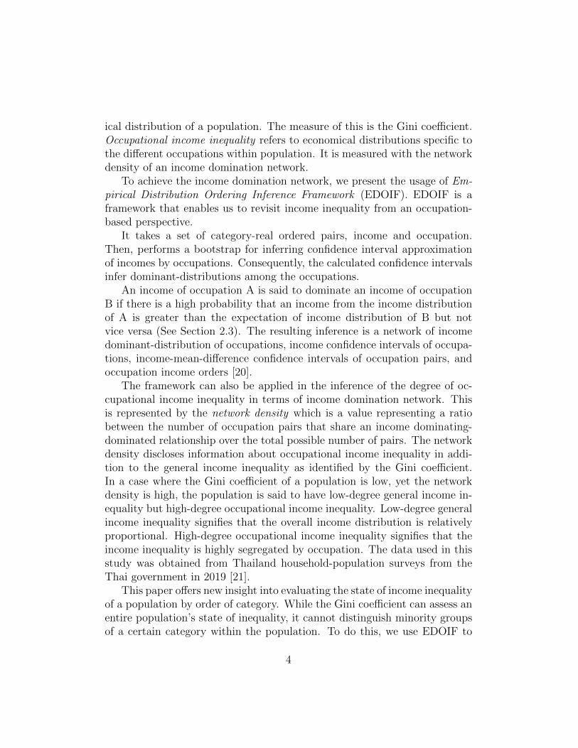
ical distribution of a population. The measure of this is the Gini coefficient.Occupational income inequality refers to economical distributions specific tothe different occupations within population. It is measured with the networkdensity of an income domination network.

To achieve the income domination network, we present the usage of Em-pirical Distribution Ordering Inference Framework (EDOIF). EDOIF is aframework that enables us to revisit income inequality from an occupation-based perspective.

It takes a set of category-real ordered pairs, income and occupation.Then, performs a bootstrap for inferring confidence interval approximationof incomes by occupations. Consequently, the calculated confidence intervalsinfer dominant-distributions among the occupations.

An income of occupation A is said to dominate an income of occupationB if there is a high probability that an income from the income distributionof A is greater than the expectation of income distribution of B but notvice versa (See Section 2.3). The resulting inference is a network of incomedominant-distribution of occupations, income confidence intervals of occupa-tions, income-mean-difference confidence intervals of occupation pairs, andoccupation income orders [20].

The framework can also be applied in the inference of the degree of oc-cupational income inequality in terms of income domination network. Thisis represented by the network density which is a value representing a ratiobetween the number of occupation pairs that share an income dominating-dominated relationship over the total possible number of pairs. The networkdensity discloses information about occupational income inequality in addi-tion to the general income inequality as identified by the Gini coefficient.In a case where the Gini coefficient of a population is low, yet the networkdensity is high, the population is said to have low-degree general income in-equality but high-degree occupational income inequality. Low-degree generalincome inequality signifies that the overall income distribution is relativelyproportional. High-degree occupational income inequality signifies that theincome inequality is highly segregated by occupation. The data used in thisstudy was obtained from Thailand household-population surveys from theThai government in 2019 [21].

This paper offers new insight into evaluating the state of income inequalityof a population by order of category. While the Gini coefficient can assess anentire population’s state of inequality, it cannot distinguish minority groupsof a certain category within the population. To do this, we use EDOIF to

4

determine the domination order of occupations and its degrees of domination.Figure 4 presents a new analysis that combines the Gini coefficient with ameasure of occupational income inequality. In the next section, the detailsof methodology are provided.

2. Methodology

2.1. Categorization of Occupations

The data provided for this study is the income of several individuals whoare the head of their households along with their occupations grouped by theprovinces of Thailand with the exception of Bangkok. The overview of thisdata can be found in the appendix.

The careers have been categorized as students (Student), animal farmer(AG-AnimalFarmer), plant farmer (AG-Farmer), fishery (AG-Fishery), or-chardist (AG-Orchardist), peasant (AG-Peasant), business owner (Business-Owner), company employee (EM-ComEmployee), company officer (EM-ComOfficer),officer (EM-Officer), freelance (Freelance), merchant (Merchant), others (Oth-ers), and unemployment (Unemployment). Wherein the careers that are as-sociated with the agricultural industry include animal farmer, farmer, fishery,orchardist, and peasant.

2.2. Agricultural Categorization of Provinces

As the agricultural sector has been referred to as the engine of growth forThailand [22], we find it appropriate to categorize the provinces of Thailandinto agricultural (AG), mixed-agricultural (mixAG), and non-agriculture (nonAG)provinces. The categories are based on the ratio of head of households. Apopulation over 66% in either AG or nonAG occupations will be catego-rized accordingly. Provinces where the population of both agriculture andnon-agriculture occupations does not exceed 66% are referred to as mixed-agricultural provinces.

2.3. Dominant-Distribution Ordering Inference

The Empirical Distribution Ordering Inference Framework (EDOIF) ap-plies Dominant-Distribution Ordering Inference. It is the inference of an or-der of domination among several categories C by utilizing the Mann-WhitneyUpper-tail Test with α = 0.05 to determine whether the distribution of cat-egory p, Dp, dominates that of category q, Dq, such that Dp � Dq. In our

5

case, we use Dominant-Distribution Ordering Inference to determine a net-work of income domination among occupations of each province in Thailandunder the null hypothesis that the income of p is less than or equal to theincome of q and, naturally, an alternate hypothesis that the the income of pis greater than the income of q [20]. The resulting dominant/non-dominantpairs are then summarized as income dominant-distribution networks for eachprovince. Note that we use a domination network as a short term for an in-come dominant-distribution network. The network density in this work referto the network density of an income dominant-distribution network, whichhas a value between 0 and 1. Higher network density implies higher numberof occupational domination pairs. Hence, we use the network density as ameasure for occupational income inequality.

2.4. Aggregation Support Network

Given the provincial domination networks as well as agricultural catego-rization of AG, mixAG, and nonAG provinces, we can now infer the Aggrega-tion Support Networks. By applying the concept of Support in AssociationRule Mining [23], the result is one network per agricultural categorization.

Let T = {ti} be a set of transactions of provinces, which are provinceseither in a specific category (i.e. AG, mixAG, or nonAG) or all provinces,in Thailand excluding Bangkok where ti is a transaction of ith province.Given X, Y are occupations, within each ti = {e(X, Y )}, e(X, Y ) ∈ ti if anincome of occupation X dominates an income of occupation Y . The supportis defined as a ratio of a number of times that an occupation pair e(X, Y )appears in any ti ∈ T divide by a number of provinces.

supp(e(X, Y )) =|{ti|ti ∈ T&e(X, Y ) ∈ ti}|

|T |(1)

Where |{ti|ti ∈ T&e(X, Y ) ∈ ti}| is a number of provinces that have anincome of occupation X dominates income of occupation Y , and |T | is anumber of provinces. With the support value of each domination pair anda support threshold of 0.5, the aggregation support networks can now beconcluded for each agricultural categorization. In the aggregation supportnetwork, the nodes are occupations and there is an edge e(X, Y ) in thenetwork if the support supp(e(X, Y )) is greater than 0.5.

6

3. Results

Through the usage of Exploratory Data Analysis, the process of inves-tigating data for patterns [24], we have created visual representations andsummary statistics to represent our findings with various forms of analyses.

This study compiles maps of Thailand displaying the locations of generalincome inequality and occupational income inequality among all provinces inThailand with the exception of the capital city of Bangkok. Additionally, thedistribution of Gini coefficients, network density, and average income rateis also calculated. Finally, among these key socioeconomic indicators, thecorrelations distinguished by agricultural provinces for Thailand in 2019 ispresented. In this work, the provinces are grouped into three types based onthe majority of occupations in provinces as explained in Section 2.2. The cat-egories are agricultural provinces (AG), non-agricultural provinces (nonAG),and mixed provinces (mixAG).

The maps of Thailand illustrate location of provinces’ Gini coefficients,average incomes, categorization of agricultural provinces, and network den-sities as shown in Figure 1.

In the aspect of occupational income inequality (Figure 1a), the areasthat have high network densities are distributed across the country. Forthe general income inequality (Figure 1b), however, the high-Gini-coefficientareas are around the upper-central provinces, the east, and the north of coun-try. In Figure 1c, the areas with high average income are around the centralof country. For agricultural types of provinces (Figure 1d), the majority ofagricultural provinces are located in Northeastern Thailand whereas non-agricultural provinces are generally clustered near the capital city, in CentralThailand, and Northwestern Thailand.

Briefly, the high-Gini-coefficient and high-average-income provinces aredistributed towards non-agricultural provinces, while high network-densityprovinces are everywhere. Figures 1a and 1b provide a clear view on dis-crepancy between network density and the Gini coefficient. For instance,Chonburi is ranked the top 5% highest network density and bottom 5% low-est Gini coefficient whereas Ranong is ranked the bottom 5% lowest networkdensity and top 5% highest Gini coefficient. This quantitatively implies thatthe network density offers insight beyond the Gini coefficient.

Since areas categorized by these four aspects—network density, Gini co-efficients, average income, and agricultural categories—that do not overlapcompletely, they play a different role in an econometric explanation of each

7

area.In Figure 2, the domination networks are presented (See Section 2.4 for

derivative). There is no significant difference among the network structure ofagricultural types of provinces. This implies that the common structure ofoccupational inequality exist for the entire country (i.e. EM officer occupa-tion dominates any occupation and the student occupation is also dominatedby any occupation in any province).

Figure 3 represents histograms of Gini coefficients, network density, andaverage incomes among provinces. In general, the network densities are no-ticeably high and between 0.78 and 0.85, the top 15% of the range, points toa feasibility that income inequality specific to distribution by occupation isa major concern as can be seen from Figure 3b. On the other hand, Figures3a and 3c display near normal distributions of Gini coefficients and averageincome histograms.

In the aspect of association among network density, Gini coefficient, andincomes, the results are shown in Figure 4. The Pearson correlation betweenthe network density and Gini coefficient is 0.17, the correlation between theGini coefficient and average income is 0.079, and finally, the correlation be-tween network density and average income is 0.049.

According to the work in Sullivan and Feinn [25], the effect sizes of theser values below 0.2 indicate small effect sizes. Thus, the measure of incomeinequality specific to occupation does not appear to be statistically relatedto the current measures of general income inequality known as the Gini coef-ficient and can therefore infer information about a population that is previ-ously unknown. To explore the significance of occupational income inequalityin comparison to general income inequality, we performed further analysisbetween the network density and Gini coefficient w.r.t. the percentage ofpopulation in the agricultural industry.

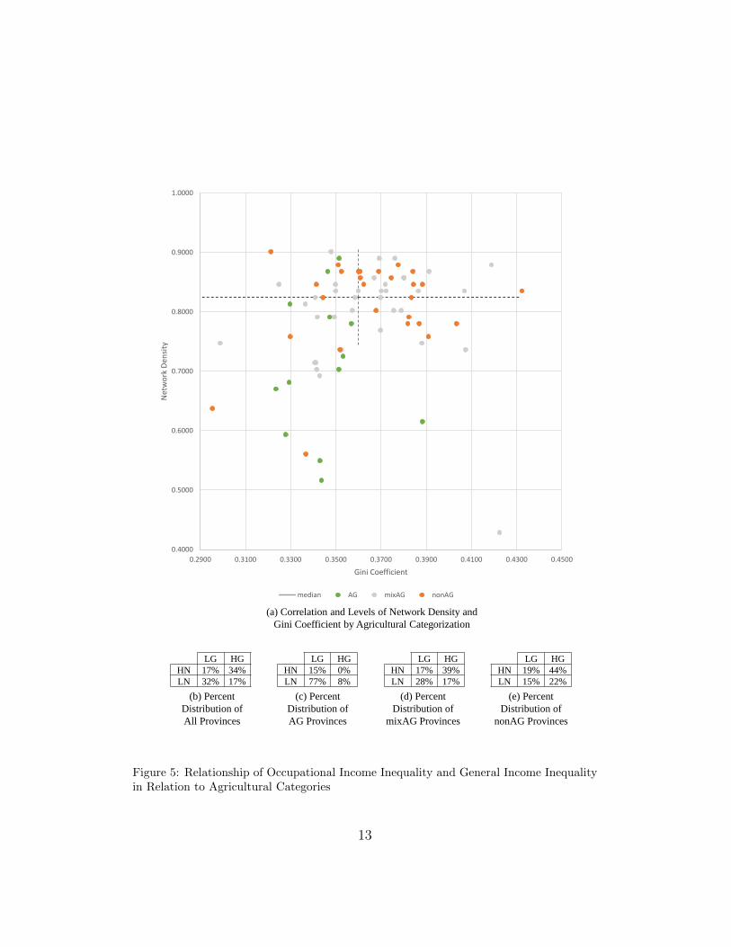
In Figure 5a, a plot of the network density and Gini coefficient distinguish-ing provinces are colored by agricultural categories. It reveals a convincingpattern between agricultural categorization and general income inequality inaddition to agricultural categorization and occupational income inequality.

The figure illustrates the provincial network density w.r.t. Gini Coeffi-cient where green indicates agricultural (AG) provinces and orange is indica-tive of non-agricultural (nonAG) provinces. The grey data points indicatemixed agricultural and non-agricultural (mixAG) provinces. The line whichdifferentiates high as opposed to low for either axes marks the median. Ac-cording to Figure 5b, 17% of all provinces in Thailand identify as populations

8

(a) Network Density

of Thailand

(b) Gini Coefficient

of Thailand

(c) Average Income

of Thailand

(d) Agricultural Provinces

of Thailand

Figure 1: Maps of Thailand depicting (a) Network Density, (b) Gini Coefficient, (c) Av-erage Income, and (d) Agricultural Provinces9

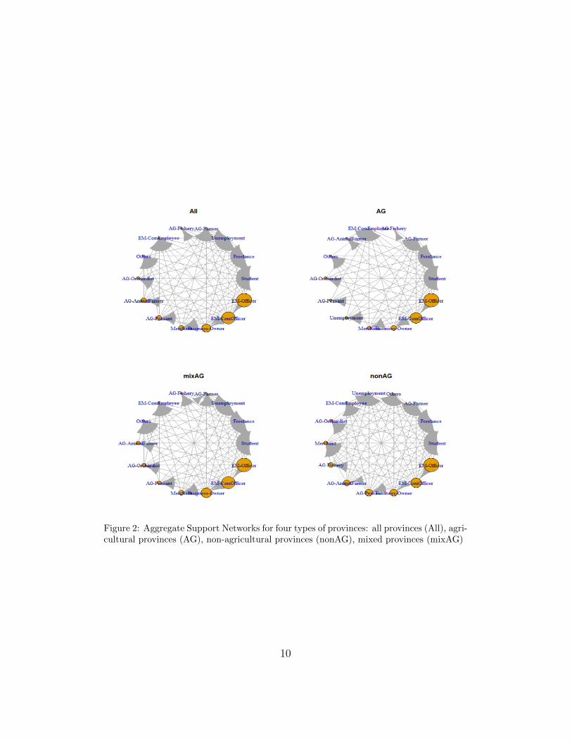
Figure 2: Aggregate Support Networks for four types of provinces: all provinces (All), agri-cultural provinces (AG), non-agricultural provinces (nonAG), mixed provinces (mixAG)

10

(a) Gini Coefficient Histogram (b) Network Density Histogram (c) Average Income Histogram

Figure 3: Frequency distribution of (a) Gini Coefficient, (b) Network Density, and (c)Average Income

(a) Scatter Plot of

Gini Coefficient and Network Density

(b) Scatter Plot of

Average Income and Gini Coefficient

(c) Scatter Plot of

Average Income and Network Density

Figure 4: Visual inspection of correlation between (a) Gini Coefficient and Network Den-sity, (b) Average Income and Gini Coefficient, and (c) Average Income and NetworkDensity

11

of low Gini coefficients (LG), and thus low-level general income inequality,yet high network density (HN), and therefore high-level occupational incomeinequality. These are provinces that would be previously indiscernible to pol-icy makers by analyzing Gini coefficient alone. Additionally, from Figure 5c,as high as 92% of all AG provinces appear to exhibit LG and among theseprovinces, 77% also exhibit low network densities (LN) implying low-level oc-cupational income inequality which suggests that AG provinces in Thailandlikely exude LGLN cases. As for nonAG provinces (Figure 5e), 66% showhigh Gini coefficients (HG) thus high-level general income inequality.

In accordance to current measures, low-level general income inequalitysuggests that the population under observation is unaffected by inequalityof income. However, when the same population exhibits high network den-sities, this points to an instance where the population seemingly has low-level inequality yet is significantly influenced by differences in occupationalinequality. This is seen in occurrence among the 17% of all provinces in Thai-land (Figures 5b), which are highly troubled with unequal wage dispersionby occupation yet undetectable by general income inequality. For instance,Songkhla province is a LGHN province.

Songkhla is a mixed-agricultural (mixAG) province (See percent distri-bution in Figure 5d). The number of occupations are relatively equally dis-tributed between agricultural and non-agricultural occupations. The lowprovincial Gini coefficient of 0.3479 shows a relatively equal distribution ofincome across the entire population. Figure 6 illustrates occupation orderingas a result of approximately 280,000 head of households in the province in2019. The income dominant occupation is ”EM-Officer” which dominatesall other occupations with an overall income above 325,000 THB or roughly9,000 USD. The high provincial network density of 0.901 demonstrates thatincome between occupations of Songkhla are highly unequally distributed.Moreover, the magnitudes of mean-difference income confidence interval ofall pairs of occupations in Songkhla from Figure 7 portrays that all the oc-cupation pairs have incomes gaps of at least 25,000 THB or about 750 USD.

On the other hand, demonstrating a province that is not significantlyaffected by income inequality generally nor by occupation-specific means, iswhere low Gini coefficients suggest low-level general income inequality andwhen these populations also show low-level occupational income inequalitywith low network densities, the population of interest is under relative idealincome conditions. For example, Amnat Charoen province is among one ofthe 77% of AG provinces in Thailand that have low-level general income

12

0.4000

0.5000

0.6000

0.7000

0.8000

0.9000

1.0000

0.2900 0.3100 0.3300 0.3500 0.3700 0.3900 0.4100 0.4300 0.4500

Net

wo

rk D

ensi

ty

Gini Coefficient

median AG mixAG nonAG

LG HG LG HG LG HG LG HG

HN 17% 34% HN 15% 0% HN 17% 39% HN 19% 44%

LN 32% 17% LN 77% 8% LN 28% 17% LN 15% 22%

(b) Percent

Distribution of

All Provinces

(c) Percent

Distribution of

AG Provinces

(d) Percent

Distribution of

mixAG Provinces

(e) Percent

Distribution of

nonAG Provinces

(a) Correlation and Levels of Network Density and

Gini Coefficient by Agricultural Categorization

Figure 5: Relationship of Occupational Income Inequality and General Income Inequalityin Relation to Agricultural Categories

13

150000

200000

250000

300000

14) S

tuden

t

13)A

G−Orch

ardis

t

12)A

G−Pea

sant

11)A

G−Anim

alFar

mer

10)A

G−Far

mer

9)Fre

elanc

e

8)Une

mploym

ent

7)AG−F

isher

y

6)Othe

rs

5)Mer

chan

t

4)EM−C

omEmplo

yee

3)Bus

iness

−Owne

r

2)EM−C

omOffic

er

1)EM−O

fficer

Categories

Val

ues

Figure 6: Income Confidence Interval of occupations in Songkhla Province

0

50000

100000

150000

200000

13)A

G−Orch

ardis

t

12)A

G−Pea

sant

11)A

G−Anim

alFar

mer

10)A

G−Far

mer

9)Fre

elanc

e

8)Une

mploym

ent

7)AG−F

isher

y

6)Othe

rs

5)Mer

chan

t

4)EM−C

omEmplo

yee

3)Bus

iness

−Owne

r

2)EM−C

omOffic

er

1)EM−O

fficer

Target Categories:B

Mea

n D

iffer

ence

s (B

min

us A

)

Based Categories:A

10)AG−Farmer11)AG−AnimalFarmer12)AG−Peasant13)AG−Orchardist14) Student2)EM−ComOfficer3)Business−Owner4)EM−ComEmployee5)Merchant6)Others7)AG−Fishery8)Unemployment9)Freelance

Figure 7: Mean-difference Income Confidence Interval of occupation pairs in SongkhlaProvince

14

100000

150000

200000

250000

300000

14) S

tuden

t

13)A

G−Fish

ery

12)E

M−Com

Employe

e

11)F

reela

nce

10)A

G−Far

mer

9)AG−O

rchar

dist

8)AG−P

easa

nt

7)Une

mploym

ent

6)Bus

iness

−Owne

r

5)Othe

rs

4)AG−A

nimalF

armer

3)EM−C

omOffic

er

2)Mer

chan

t

1)EM−O

fficer

Categories

Val

ues

Figure 8: Income Confidence Interval of occupations in Amnat Charoen Province

inequality and also show low-level occupational income inequality.Amnat Charoen is an AG province whose mild gaps of occupational in-

come inequality is illustrated in Figures 8 and 9. With a low Gini coef-ficient of 0.3437, the income distribution of the province is fairly equallydistributed. The occupation ordering shows that the dominant occupationis ”EM-Officer” with an overall income above 300,000 THB or roughly 8,900USD. The low provincial network density of 0.517 suggests that incomebetween occupations are relatively equally distributed throughout AmnatCharoen. The magnitudes of mean-difference income confidence interval ofmost pairs of occupations portrays that income gaps of all occupation pairsare at least 50,000 THB or about 1500 USD. Comparing against SongkhlaProvince, Amnat Charoen has less number of income inequality of occupationpairs but when it has a gap, it has larger gaps of income.

Given that the null hypothesis states the agricultural categories of provincesis independent to the low-high categories of the Gini coefficient and networkdensity, the alternative hypothesis states that the two are dependent. AChi-Square Independence Test with the significant level α = 0.05 supportsthat the categorizations of AG provinces and their corresponding low-highGini coefficient and network density are not independent of each other. Thissupports the assumptions from our above statements that AG provinces areassociated with low general income inequality and nonAG provinces are as-

15

0e+00

1e+05

2e+05

13)A

G−Fish

ery

12)E

M−Com

Employe

e

11)F

reela

nce

10)A

G−Far

mer

9)AG−O

rchar

dist

8)AG−P

easa

nt

7)Une

mploym

ent

6)Bus

iness

−Owne

r

5)Othe

rs

4)AG−A

nimalF

armer

3)EM−C

omOffic

er

2)Mer

chan

t

1)EM−O

fficer

Target Categories:B

Mea

n D

iffer

ence

s (B

min

us A

)

Based Categories:A

10)AG−Farmer11)Freelance12)EM−ComEmployee13)AG−Fishery14) Student2)Merchant3)EM−ComOfficer4)AG−AnimalFarmer5)Others6)Business−Owner7)Unemployment8)AG−Peasant9)AG−Orchardist

Figure 9: Mean-difference Income Confidence Interval of occupation pairs in AmnatCharoen Province

sociated with high general income inequality yet for occupational income in-equality only AG provinces show significant favor towards low occupationalincome inequality.

4. Discussion

The findings in this study distinguish the provinces of Thailand intogroups characterized by levels of general and occupational income inequality.A combination of two groups show results that suggest an ideal condition forlowering overall income inequality in Thailand and perhaps other countrieswith similar measurement index results. When general income inequality isunsubstantial and occupational income inequality is serious, such as the caseof Songkhla shown in Figures 6 and 7, the condition of income inequalityis misleading to residents and policy makers. This supports the statementthat inter-occupational inequality is a significant aspect of income inequalitythat should not be overlooked [26]. On the other hand, when both the gen-eral and occupational income inequality is low as is in Figures 9, this pointsto a province with ideal living conditions where rates of unemployment iscomparatively lower and overall income inequality is low-level.

The Harris-Todaro Migration Model is a predictive model that explains

16

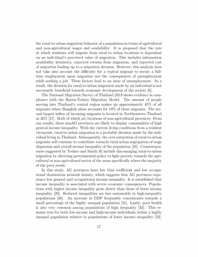
the rural-to-urban migration behavior of a population in terms of agriculturaland non-agricultural wages and availability. It is proposed that the rateat which residents will migrate from rural to urban locations is dependenton an individual’s perceived value of migration. This includes informationavailability heuristics, expected returns from migration, and expected costof migration leading up to a migration decision. However, this analysis doesnot take into account the difficulty for a typical migrant to secure a full-time employment upon migration nor the consequences of unemploymentwhile seeking a job. These factors lead to an issue of unemployment. As aresult, the decision for rural-to-urban migration made by an individual is notnecessarily beneficial towards economic development of the society [6].

The National Migration Survey of Thailand 2019 shows evidence in com-pliance with the Harris-Todaro Migration Model. The amount of peoplemoving into Thailand’s central region makes up approximately 45% of allmigrants where Bangkok alone accounts for 19% of these migrants. The sec-ond largest influx of incoming migrants is located in Northeastern Thailandat 26% [27]. Both of which are locations of non-agricultural provinces. Fromour results, these nonAG provinces are likely to display communities of highgeneral income inequality. With the current living conditions from a residentviewpoint, rural-to-urban migration is a probable decision made by the indi-vidual living in Thailand. Subsequently, the over-saturation of rural-to-urbanmigrants will continue to contribute towards rural-urban segregation of wagedispersion and overall income inequality of the population [28]. Countermea-sures suggested by Todaro and Smith [6] include discouraging rural-to-urbanmigration by directing governmental policy to fight poverty towards the agri-cultural or non-agricultural sector of the areas specifically where the majorityof the poor reside.

In this study, AG provinces have low Gini coefficient and low occupa-tional domination network density, which suggests that AG provinces expe-rience low general and occupational income inequality. It is established thatincome inequality is associated with severe economic consequences. Popula-tions with higher income inequality grow slower than those of lower incomeinequality [29]. Reduced inequalities are less sustainable in high-inequalitypopulations [30]. An increase in GDP frequently concentrates towards asmall percentage of the highly unequal population [31]. Lastly, poor healthis also very common among populations of high inequality [32]. This re-mains true for both low-income and high-income individuals within a highlyunequal population relative to populations of lower income inequality [33].

17

Therefore, areas of low general and occupational income inequality (i.e. AGprovinces) may be a suitable area for policy makers to encourage residentsremain. This is consistent with the Harris-Todaro Migration Model.

From the perspective of the policy makers, the Gini coefficient cannotindicate where the majority lies in terms of general income inequality butthe usage of EDOIF to analyze occupational income inequality allows us tosee minority groups by order of income oppression. Among the majority ofincome confidence intervals of all provinces, there exists a global structurethat remains intact throughout. ”Student” and ”EM-Officer”, for the mostpart, rank most and least dominated, respectively throughout Thailand. Byacknowledging both measurement indices, policy makers can utilize this in-formation to develop policies that leaves no minority behind.

5. Conclusion

This study investigated how occupational income inequality provides in-sight into general income inequality as measured by the Gini coefficient. Ourstudy showed that most agricultural provinces display ideal levels of both oc-cupational and general equality in comparison to non-agricultural provinceswhich tend to experience a strong indication of general income inequality.Moreover, some non-agricultural provinces show the degree of high occu-pational income inequality even if they have low general income inequality.Despite these conditions, the Thai population still frequently choose to mi-grate towards the locations of growing income inequality for individual gain.Thus, occupational income inequality can be utilized to assist policy mak-ers in decision-making for economic development. From our best knowledge,a solution may be to align the benefits of individuals to those of the na-tional economy. This might be by supporting minority occupations in areasof massive inequality. For example, students, who face income inequality is-sue, residing in areas of high occupational income inequality might get moresupport. Policy makers can also discourage rural-to-urban migration by dis-tributing the benefits of rural income to a wider audience so that the optionnaturally becomes more alluring to individuals.

References

[1] D. Anantanasuwong, Income distribution and socio-economic disparityin aging society in thailand, 社会システム研究 39 (2019) 27–42.

18

[2] U. N. D. of Economic, S. Affairs, The Sustainable Development GoalsReport 2021, 2021 ed., United Nations, 2021. URL: https://www.

un-ilibrary.org/content/books/9789210056083.

[3] R. Jolly, The world employment conference: The enthronement of ba-sic needs, Development Policy Review A9 (1976) 31–44. URL: https://doi.org/10.1111/j.1467-7679.1976.tb00338.x. doi:10.1111/j.1467-7679.1976.tb00338.x.

[4] P. Streeten, Basic human needs, Millennium: Journal of Inter-national Studies 7 (1978) 29–46. URL: https://doi.org/10.1177/

03058298710010010301. doi:10.1177/03058298710010010301.

[5] B. E. Moon, W. J. Dixon, Politics, the state, and basic human needs:A cross-national study, American Journal of Political Science 29 (1985)661–694. URL: http://www.jstor.org/stable/2111176.

[6] M. P. Todaro, S. C. Smith, Economic Development, 12th Edition, 12ed., Pearson, 2015.

[7] F. M. Nafukho, N. Hairston, K. Brooks, Human capital theory: im-plications for human resource development, Human Resource Devel-opment International 7 (2004) 545–551. URL: https://doi.org/10.

1080/1367886042000299843. doi:10.1080/1367886042000299843.

[8] G. S. Becker, Human Capital: A Theoretical and Empirical Analysis,with Special Reference to Education, 3 ed., The University of ChicagoPress, 1993.

[9] J. Mincer, Investment in human capital and personal in-come distribution, Journal of Political Economy 66 (1958) 281–302. URL: https://doi.org/10.1086/258055. doi:10.1086/258055.arXiv:https://doi.org/10.1086/258055.

[10] F. G. De Maio, Income inequality measures, Journal of Epidemiologyand Community Health 61 (2007) 849–852. URL: https://jech.bmj.com/content/61/10/849. doi:10.1136/jech.2006.052969.

[11] Y. Xu, X. Qiu, X. Yang, G. Chen, Factor decomposition of the changesin the rural regional income inequality in southwestern mountainous

19

area of china, Sustainability 10 (2018) 3171. URL: https://doi.org/10.3390/su10093171. doi:10.3390/su10093171.

[12] P. Phongpaichit, Inequality, wealth and thailand’s politics, Journalof Contemporary Asia (2016) 405–424. doi:10.1080/00472336.2016.1153701.

[13] A. Booth, Measuring poverty and income distribution in southeast asia,Asian-Pacific Economic Literature 33 (2019) 3–20. URL: https://doi.org/10.1111/apel.12250. doi:10.1111/apel.12250.

[14] P. Meneejuk, W. Yamaka, Analyzing the relationship between incomeinequality and economic growth: Does the kuznets curve exist in thai-land?, 2016.

[15] N. Wasi, S. W. Paweenawat, C. D. N. Ayudhya, P. Treeratpituk,C. Nittayo, Labor Income Inequality in Thailand: the Roles of Edu-cation, Occupation and Employment History, PIER Discussion Papers117, Puey Ungphakorn Institute for Economic Research, 2019. URL:https://ideas.repec.org/p/pui/dpaper/117.html.

[16] Global Wealth Databook 2020, CreditSuisse, 2020.

[17] O. of the National Economic, S. D. Council, Gross domestic product :Q2/2021, 2021. URL: https://www.nesdc.go.th/, date accessed: 26October 2021.

[18] O. of the National Economic, S. D. Council, National income of thailand2019 chain volume measures, 2021. URL: https://www.nesdc.go.th/,date accessed: 26 October 2021.

[19] N. S. O. of Thailand, Core economic indicators of thailand (1998-2002),http://web.nso.go.th/, 2002. Accessed: 2020-09-13.

[20] C. Amornbunchornvej, N. Surasvadi, A. Plangprasopchok, S. Tha-jchayapong, A nonparametric framework for inferring orders of cate-gorical data from category-real pairs., Heliyon 6 (2020) e05435. URL:https://doi.org/10.1016/j.heliyon.2020.e05435. doi:10.1016/j.heliyon.2020.e05435.

20

[21] C. Amornbunchornvej, N. Surasvadi, A. Plangprasopchok, S. Tha-jchayapong, Identifying linear models in multi-resolution populationdata using minimum description length principle to predict householdincome, ACM Transactions on Knowledge Discovery from Data (TKDD)15 (2021) 1–30.

[22] N. Poapongsakorn, M. Ruhs, S. Tangjitwisuth, Problems and outlookof agriculture in thailand, Thailand Development Research InstituteQuarterly Review 13 (1998).

[23] C. Zhang, S. Zhang, Association Rule Mining: Models and Algorithms,Springer-Verlag, Berlin, Heidelberg, 2002.

[24] P. Diaconis, Theories of Data Analysis: From Magical Think-ing Through Classical Statistics, 2011, pp. 1–36. doi:10.1002/9781118150702.ch1.

[25] G. M. Sullivan, R. Feinn, Using effect size—or why the p value is notenough, Journal of Graduate Medical Education 4 (2012) 279–282.URL: https://doi.org/10.4300/jgme-d-12-00156.1. doi:10.4300/jgme-d-12-00156.1.

[26] G. Kambourov, I. Manovskii, Occupational mobility and wage in-equality, The Review of Economic Studies 76 (2009). URL: http:

//www.jstor.org/stable/40247619.

[27] N. S. O. of Thailand, National migration survey of thailand (2019), 2019.Http://www.nso.go.th/sites/2014en/.

[28] M. A. Reda, L. Hohfeld, S. Jitsuchon, H. Waibel, Rural-urban migrationand employment quality: A case study from thailand, 2012.

[29] N. R. Buttrick, S. Oishi, The psychological consequences of incomeinequality, Social and Personality Psychology Compass 11 (2017).doi:https://doi.org/10.1111/spc3.12304, e12304 SPCO-0790.R3.

[30] J. Ostry, A. Berg, Inequality and unsustainable growth: Two sidesof the same coin?, Staff Discussion Notes 11 (2011) 1. doi:10.5089/9781463926564.006.

21

[31] T. Piketty, E. Saez, Inequality in the long run, Technical Re-port, HAL, 2014. URL: https://EconPapers.repec.org/RePEc:hal:pseose:halshs-01053609.

[32] K. Pickett, R. Wilkinson, Income inequality and health: A causal re-view, Social science and medicine (1982) 128 (2014). doi:10.1016/j.socscimed.2014.12.031.

[33] S. Subramanian, I. Kawachi, Being well and doing well: on the im-portance of income for health, International Journal of Social Wel-fare 15 (2006) S13–S22. doi:https://doi.org/10.1111/j.1468-2397.2006.00440.x.

22