1

Obtaining the speed of light using the Foucault Method and the PASCO apparatus.

Quintin T. Nethercott and M. Evelynn Walton

University of Utah Department of Physics and Astronomy

Advanced Undergraduate Lab

March 23, 2013 In this experiment the speed of light was obtained and verified against the accepted value of 2.99792458 x 108 m/s using the Foucault method and the PASCO optics apparatus. The experiment served to provide insight into the most important constant in physics as well as an opportunity to explore the methods used by Albert Michelson, who was able to measure the speed of light using Foucault’s rotating mirror method. The speed of light, c, found by this group using a linear regression model was (2.9 +/- 0.1) x 108 m/s.

I. INTRODUCTION

The speed of light has an important role in physics. It places a limit on how fast an object can travel since no mass has been observed to move at the rate of light. The speed of light remains constant, regardless of the frame of reference an observer is in. Until the seventeenth century the speed of light was thought to be infinite by many astronomers. Galileo tried unsuccessfully to quantify c with the use of shuttered lanterns on hilltops. Danish astronomer Olaf Roemer used the eclipse of one of Jupiter’s moon the find the value 2.14 x 108 m/s [1]. In the 18th century the French physicists Fizeau and Foucault developed an optics apparatus that found the value for c to within a 5% error [1]. Michelson was able to refine the Foucault method to find a value for c that won him the Nobel Prize in 1907 and gave the world a value that has become the accepted standard for the SI unit of distance; the time it takes light to travel one meter: 1m = 1/2.99792458e8 seconds [1].

The speed of light also emerges from the inverse square root of the products of the permittivity and permeability constants in Maxwell’s equations where c is the speed of light in vacuum as shown in the following equation:

√

(1)

2

This discovery was one of the most exciting moments in physics; the laws of electromagnetism were united with the properties of light leading to profound discoveries of the nature of photons.

A. THEORETICAL INTRODUCTION

This experiment uses the Foucault method to find the speed of light in the Undergraduate Lab at the University of Utah. With the PASCO manual and the optics equipment the relationship between the speed of light and the displacement of the image, Δs’, in the measuring microscope can be determined [Fig. 1].

Figure 1. The Foucault Method schematics [2].

The following quantities and variables are also used: the rate of rotation of the mirror (ω), the distance between the fixed mirror and the rotating mirror (D), the distance between lens 1 and lens 2 (A), and the distance between lens 2 and the rotating mirror(B). The optical path starts at the laser with the light being focused to a point s at the focal length of L1. The image of s is reflected from MR onto MF and then reflected back on the same path to the image point s. The beam splitter places a reflected image of the returning light at point s’. When MR is rotating very quickly the image points s and s’ are moved [2] because the distance S is different from S1 as shown in Figure 2. The expression for ΔS in terms of D and θ:

( ) [ ( ) ] (2) Figure 2 shows the image shifting on the fixed mirror and the subsequent change in the reflection of s’ on the beam splitter. It shows the virtual image of the fixed mirror which helps visualize the effect the rotating mirror has on the reflected image s’.

3

Since the mirror is in a different position once the reflected beam gets back to MR the location of s’ is different; the difference Δs’ is focused in the plane of point s with a height that is proportional to the ratio of the image and object distances from L2[2].

The expression for displacement of the image point Δs’ can be written in terms of the measured distances between lenses and mirrors:

(3)

Figure 2. Analyzing the shift in images [2]. Combining equations (2) and (3) and using ΔS = S1-S the expression for Δs’ can then be written using Δθ:

(4)

The angle Δθ is dependent on the angular velocity of the rotating mirror and on the time it takes for the beam to reflect between both mirrors for a total distance 2D and the time it takes for the light to travel from the rotating mirror to the fixed mirror and back to the beam splitter. Δθ can be expressed as a function of ω and c:

4

(5)

Replacing Δθ in Eq. 5 gives the displacement of the beam in terms of the speed of light.

( ) (6)

Then c can be found from measured values Δs’ and ω by rearranging Eq. 6.

( ) (7)

Figure 2 shows the values A, B, and D. The values Δs’ and ω are variable in

each trial. Eq. 6 shows that a linear relation between Δs’ and ω exists and that a least linear square fit can be applied to calculate the slope m, which provides another method of calculating c. Eq. 8 shows this relation:

( ) (8)

The value Δs’ is taken from two separate measurements of the displacement; one from a value of ω in one direction and the other from the value of ω in the opposite direction. This has the effect of halving the error in δs.

II. EXPERIMENTAL SETUP

The optics bench is made up of several components that must be carefully aligned per manual instructions; high speed rotating mirror assembly, a concave fixed mirror, a measuring microscope, a 0.5mW He-Ne laser, two lenses of focal length 48mm and 252mm, and a set of polarizers. The setup is described in Figure 3 as well as painstakingly detailed in the PASCO manual [2].

5

Figure 3. Optics bench components and alignment [2].

Proper alignment was of utmost importance in finding the correct image in the microscope. The manual details the correct step-by-step setup. The optics bench was leveled and the laser placed on the right-hand side of the bench. The rotating mirror was placed on the opposite end of the bench and aligned at 17cm. The laser was then aligned so the beam would strike the center of MR using the included alignment jigs. The beam was then directed back to the laser. Lenses were then mounted with careful attention to centering the laser beam each time. The measuring microscope was mounted at mark 82.0 cm and the beam was centered on the rotating mirror again. The fixed mirror was placed at the end of the lab bench about 4 meters away from the optics bench at an angle around 15 degrees from the rotating mirror (Fig. 4 and 5).

Figure 4. Optics bench with all components.

6

Figure 5. Optics bench(near) and fixed mirror (far).

The laser beam was then directed to the fixed mirror MF by moving the rotating mirror by hand. The fixed mirror was then adjusted so the beam was directed back at the center of MR ; this took the skill and patience of two people: one adjusting the fixed mirror while the other guided from the rotating mirror. Once the alignment was finished the image of the beam appeared as a spot in the microscope and could be viewed when the polarizers were in place for eye protection. The crosshairs were adjusted to be centered on the beam spot in preparation for the mirror to start rotating. The adjustments were made from the microscope and the micrometer knob gave the distance of adjustment with an accuracy of 0.5 μm. There were some options involving adjustments of lenses for “cleaning up” of the spot image. Some diffraction patterns were visible, but the image was very good in this case [2].

III. EXPERIMENTAL PROCEDURE In order to experimentally calculate a value for c measurements at ten different ω were taken: 1520 (the maximum for the motor-driven mirror), 1335, 1181, 1017, 865, 731, 604, 467, 320, and 319 (values are in rev/sec with an uncertainty of +/- 1 rev/sec). For each ω the initial position of the spot image was measured, the motor which spins the mirror was then turned on and the new position of the spot image was measured, then the rotation was reversed and the new position of the spot image was again measured. Δs’ was determined by

7

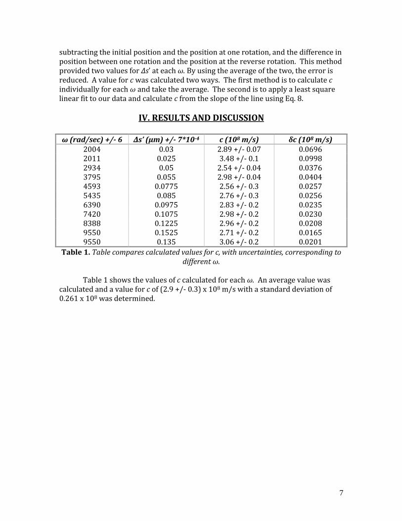
subtracting the initial position and the position at one rotation, and the difference in position between one rotation and the position at the reverse rotation. This method provided two values for Δs’ at each ω. By using the average of the two, the error is reduced. A value for c was calculated two ways. The first method is to calculate c individually for each ω and take the average. The second is to apply a least square linear fit to our data and calculate c from the slope of the line using Eq. 8.

IV. RESULTS AND DISCUSSION

ω (rad/sec) +/- 6 Δs’ (µm) +/- 7*10-4 c (108 m/s) δc (108 m/s) 2004 0.03 2.89 +/- 0.07 0.0696 2011 0.025 3.48 +/- 0.1 0.0998 2934 0.05 2.54 +/- 0.04 0.0376 3795 0.055 2.98 +/- 0.04 0.0404 4593 0.0775 2.56 +/- 0.3 0.0257 5435 0.085 2.76 +/- 0.3 0.0256 6390 0.0975 2.83 +/- 0.2 0.0235 7420 0.1075 2.98 +/- 0.2 0.0230 8388 0.1225 2.96 +/- 0.2 0.0208 9550 0.1525 2.71 +/- 0.2 0.0165 9550 0.135 3.06 +/- 0.2 0.0201

Table 1. Table compares calculated values for c, with uncertainties, corresponding to different ω.

Table 1 shows the values of c calculated for each ω. An average value was calculated and a value for c of (2.9 +/- 0.3) x 108 m/s with a standard deviation of 0.261 x 108 was determined.

8

Figure 6. Linear regression for c proportional to 1/slope. Figure 6 shows the plotted values of Δs’ and ω, along with the linear fit. The least squares linear fit gives a value of (1.48224 +/- 0.0674) x 10-5 s/mm for the slope, and 0.00159 +/- 0.00422 for the y-intercept. The R-square value for the fit is 0.98172. From the slope c can be calculated using Eq. 8, and a value of (2.9 +/- 0.1) x 108 m/s was determined.

9

Figure 7. Residual graph showing random distribution of error.

The residual graph of the data is shown in Figure 7. Although, the data points do not pass through zero, they do show randomness and are a good candidate for a linear fit. Also, the R-square value is close to 1, which means that the linear fit is a sufficient model for the data. The two values of c which were calculated are both within one standard deviation from the accepted value of 2.99792458 x 108 m/s. Of the two methods, the least square linear fit provided a more accurate result with a smaller uncertainty.

V. CONCLUSION In conclusion, by using the Foucault method, the PASCO optics apparatus, and a least squares linear fit the speed of light was successfully calculated to be (2.9 +/- 0.1) x 108 m/s. The two methods of calculating c utilized, taking the average of individually calculated values and using the slope of a least squares linear fit, provided values within one standard deviation of the accepted value for c (2.99792458 x 108 m/s). However, the least squares linear fit method provided a more accurate result and helped to reduce the uncertainty in the calculated value. The uncertainty was also reduced by taking measurements for opposite rotations. Further improvements in the experiment could be made by more accurate measurements of the distances, and a larger spread of the rotational speed of the mirror.

10

VI. REFERENCES [1] Clintberg, Brian. “Speed of Light”. March 25, 2013. http://www.studyphysics.ca/ [2] Lee, Bruce. “Instruction Manual and Experiment Guide: Speed of Light Apparatus.” PASCO Scientific.

APPENDIX. Error Analysis

The error associated with this experiment is as follows: For the value of c from ten different measurements over an order of magnitude using Δs’, ω, A, B, and D:

√(

) (

) (

) (

) (

) (a)

The uncertainty in Δs’ is determined from error propagation for the expression for Δs’:

(b)

where sf is the measurement of the second displacement from center using the reversed angular velocity and si is the measurement from the first displacement. Taking two measurements of the displacement reduces the error by 30% in Δs’.

√(

)

(

)

(c)

The error in each measurement of displacement was half a micrometer for precision of the instrument and half a micrometer for the judgment of the microscope user. The error in the linear regression was calculated by propagating the errors in A, B, D, and the slope of the line m obtained from graphing Δs’ and ω.

√(

) (

) (

) (

) (d)