Observing Unobservables: Identifying Information ...webfac/emiguel/e271_s05/karlan.pdf · Observing...
59
Observing Unobservables: Identifying Information Asymmetries with a Consumer Credit Field Experiment Dean S. Karlan* Princeton University, M.I.T. Poverty Action Lab Jonathan Zinman * Federal Reserve Bank of New York February 26 th , 2005 ABSTRACT Information asymmetries are important in theory but difficult to identify in practice. We estimate the empirical importance of adverse selection and moral hazard in a consumer credit market using a new field experiment methodology. We randomized 58,000 direct mail offers issued by a major South African lender along three dimensions: 1) the initial "offer interest rate" appearing on the direct mail solicitations; 2) a "contract interest rate" equal to or less than the offer interest rate and revealed to the over 4,000 borrowers who agreed to the initial offer rate; and 3) a dynamic repayment incentive that extends preferential pricing on future loans to borrowers who remain in good standing. These three randomizations, combined with complete knowledge of the Lender's information set, permit identification of specific types of private information problems. Specifically, our setup distinguishes adverse selection from moral hazard effects on repayment, and thereby generates unique evidence on the existence and magnitudes of specific credit market failures. We find some evidence of both adverse selection and moral hazard, and the findings suggest that about 20% of default is due to asymmetric information problems. This helps explain the prevalence of credit constraints even in a market that specializes in financing high-risk borrowers at very high rates. * [email protected], [email protected]. The views expressed herein are those of the authors and do not necessarily reflect those of the Federal Reserve Bank of New York or the Federal Reserve System. We are grateful to the National Science Foundation (SES-0424067) and BASIS/USAID (CRSP) for funding research expenses, and the Lender for financing the loans. Jeff Arnold, Jonathan Bauchet, Lindsay Dratch, Tomoko Harigaya, Kurt Johnson, Karen Lyons, and Marc Martos-Vila provided excellent research assistance. Thanks also to Abhijit Banerjee, Esther Duflo, Amy Finkelstein, Douglas Gale, Stefan Klonner, Andreas Lehnert, Ted Miguel, Rohini Pande, Michel Robe, Chris Udry, and numerous seminar and conference participants for helpful comments and discussions. Above all we thank the management and staff of the cooperating Lender for implementing the experimental protocols.
-
Upload
trinhthien -
Category
Documents
-
view
221 -
download
2
Transcript of Observing Unobservables: Identifying Information ...webfac/emiguel/e271_s05/karlan.pdf · Observing...

Observing Unobservables: Identifying Information Asymmetries
with a Consumer Credit Field Experiment
Dean S. Karlan*
Princeton University, M.I.T. Poverty Action Lab
Jonathan Zinman* Federal Reserve Bank of New York
February 26th, 2005
ABSTRACT
Information asymmetries are important in theory but difficult to identify in practice. We estimate the empirical importance of adverse selection and moral hazard in a consumer credit market using a new field experiment methodology. We randomized 58,000 direct mail offers issued by a major South African lender along three dimensions: 1) the initial "offer interest rate" appearing on the direct mail solicitations; 2) a "contract interest rate" equal to or less than the offer interest rate and revealed to the over 4,000 borrowers who agreed to the initial offer rate; and 3) a dynamic repayment incentive that extends preferential pricing on future loans to borrowers who remain in good standing. These three randomizations, combined with complete knowledge of the Lender's information set, permit identification of specific types of private information problems. Specifically, our setup distinguishes adverse selection from moral hazard effects on repayment, and thereby generates unique evidence on the existence and magnitudes of specific credit market failures. We find some evidence of both adverse selection and moral hazard, and the findings suggest that about 20% of default is due to asymmetric information problems. This helps explain the prevalence of credit constraints even in a market that specializes in financing high-risk borrowers at very high rates.
*[email protected], [email protected]. The views expressed herein are those of the authors and do not necessarily reflect those of the Federal Reserve Bank of New York or the Federal Reserve System. We are grateful to the National Science Foundation (SES-0424067) and BASIS/USAID (CRSP) for funding research expenses, and the Lender for financing the loans. Jeff Arnold, Jonathan Bauchet, Lindsay Dratch, Tomoko Harigaya, Kurt Johnson, Karen Lyons, and Marc Martos-Vila provided excellent research assistance. Thanks also to Abhijit Banerjee, Esther Duflo, Amy Finkelstein, Douglas Gale, Stefan Klonner, Andreas Lehnert, Ted Miguel, Rohini Pande, Michel Robe, Chris Udry, and numerous seminar and conference participants for helpful comments and discussions. Above all we thank the management and staff of the cooperating Lender for implementing the experimental protocols.

2
I. Introduction
Information asymmetries are often believed to cause credit market failures. Stiglitz and
Weiss (1981) sparked a large literature of theoretical papers on the role of asymmetric information
in credit markets; this literature has influenced economic policy and practice worldwide. These
theories show that information frictions and ensuing credit market failures can produce harmful
real consequences at both the micro and the macro level, via underinvestment (Gale 1990; Banerjee
and Newman 1993; Hubbard 1998), overinvestment (de Meza and Webb 1987; Bernanke and
Gertler 1990), or poverty traps (Mookherjee and Ray 2004).
Yet empirical evidence on the existence and importance of specific information frictions is
relatively thin (Chiappori and Salanie (2003)).1 Distinguishing between adverse selection and
moral hazard is difficult even when precise data on underwriting criteria and clean variation in
contract terms are available, as a single interest rate (or insurance contract) may produce
independent, conflated selection and incentive effects.2 For example, a positive correlation
between default and a randomly assigned interest rate, conditional on observable risk, could be due
to ex-ante adverse selection (those with relatively high probabilities of default will be more likely
to accept a high rate) or ex-post moral hazard (because those given high rates have greater incentive
to default).
More generally, despite widespread interest in liquidity constraints and their real effects,
empirical evidence on the existence of any specific credit market failure is lacking. Consequently
1 Note also that the 2001 Nobel Prize Committee’s citation for pioneering work on asymmetric information did not cite any empirical work on credit markets, while citing six empirical papers on labor markets and four on insurance markets (Bank of Sweden 2001). 2 See Ausubel (1999) for a related discussion of the problem of disentangling adverse selection and moral hazard in a consumer credit market. See Chiappori and Salanie (2000) and Finkelstein and McGarry (2003) for approaches to the analogous problem in insurance markets.

3
there is little consensus on the importance of liquidity constraints for individuals.3 Empirical work
typically has examined this issue indirectly,4 either through accounting exercises which calculate
the fixed and variable costs of lending, or by inferring credit constraints by from an agent’s ability
to smooth consumption and/or income (e.g., Morduch (1994)). But these indirect approaches do
not produce microfoundations in specific credit market failures. In fact, work studying the impact
of credit market failures on the real economy tends to take some reduced-form credit constraint as
given (e.g., Wasmer and Weil (2004)), or as a hypothesis to be tested (e.g., Banerjee and Duflo
(2004)), without evidence of a specific friction that may (or may not) actually produce a sub-
optimal allocation of credit. Our work provides microfoundations for studying the real effects of
credit constraints by identifying the presence (or absence) and magnitudes of two specific credit
market failures: adverse selection and moral hazard.
We test for the presence of distinct types of hidden information problems using a new
experimental methodology that disentangles adverse selection from moral hazard effects on
repayment. This market field experiment was implemented by a South African firm specializing in
high-interest, unsecured term lending to poor workers. The experiment identifies information
asymmetries by randomizing loan pricing along three dimensions: first on the interest rate offered
on a direct mail solicitation, second on the actual interest rate on the loan contract, and third on the
interest rate offered on future loans.5
A stylized example, illustrated in Figure 1, captures the heart of our methodology.
Potential borrowers with the same observable risk are randomly offered a high or a low interest rate
on a direct-mail solicitation. Individuals then decide whether to borrow at the solicitation’s “offer”
rate. Of those that respond to the high rate, half are randomly given a new lower “contract” interest 3 The empirical importance of credit market failures for firms is also debated; see, e.g., Hurst and Lusardi (2004) and Banerjee and Duflo (2004). 4 See Morduch and Armendariz de Aghion (2005) for a discussion of this literature. 5 The Lender assumed all of the revenue and repayment risk from these pricing changes. Some implementation and operational costs were shared with the authors, e.g., training and project management. Although the Lender typically employs direct mail solicitation to market to former clients, they have not in the past included price in their letters.

4
rate, while the remaining half continue to receive the high rate (i.e., their contract rate equals the
offer rate). Individuals do not know beforehand that the contract rate may differ from the offer
rate. Any selection effect is identified by considering the sample that received the low contract
rate, and comparing the repayment performance of those who responded to the high offer interest
rate with those who responded to the low offer interest rate. This follows from the fact that
although everyone in this hypothetical sample was randomly assigned identical contracts, they
selected in at varying, randomly assigned rates, so any difference in repayment is attributable to
selection on unobservables. Similarly, any effect of repayment burden (which includes moral
hazard)6 is identified by considering the sample that responded to the high offer interest rate, and
comparing the repayment performance of those who received the high contract interest rate with
those who received the low contract interest rate. These borrowers selected in identically, but
ultimately received randomly different interest rates on their contract, and any difference in default
is attributable to the resulting repayment burden.
Next, after all terms (loan amount, length of loan, and interest rate) are finalized, we
randomize whether the contract interest rate applies to the initial loan only, or instead to all loans
within a one year period, conditional on good repayment. The yearlong assignment explicitly
raises the benefits of repaying the current loan on time (in the 98% of cases where the contract rate
is less than the Lender’s standard rate). Moreover, this “dynamic repayment incentive” does not
change the costs of repaying the initial loan; initial debt burden is unperturbed. Any correlation
between this incentive and default therefore must be driven by choices—pure moral hazard. The
dynamic repayment incentive thus yields our sharpest test for the presence of moral hazard.
6 We define moral hazard as the effect of repayment burden on repayment that stems from ex-post behavioral changes driven by the incentives of the contract. Repayment burden also includes a mechanical wealth or income effect: those with positive (negative) shocks to wealth or income will be more (less) able to repay higher interest debt. Section IV discusses this in more detail.

5
Our approach to estimating the extent and nature of asymmetric information is thus most
similar in intent to Edelberg (2004), and in methodology to Ausubel (1999).7 Edelberg estimates a
structural model to disentangle the effects of adverse selection and one type of moral hazard (in
effort) in collateralized consumer credit markets in the United States. She finds evidence
consistent with both phenomena. Ausubel uses market experiments conducted by a large American
credit card lender to estimate the extent and nature of adverse selection. He does not attempt to
account for moral hazard separately, arguing that any such effect must be trivially small over the
range of interest rates (800 basis points per annum) contracted on in his data.
We also examine whether the pattern of information asymmetries varies with the gender of
the borrower, since 75% of microcredit clients worldwide are women (Microcredit Summit
Campaign 2003). Microlending institutions have targeted women for several reasons, including
their relatively reliable repayment behavior. Women are better microcredit risks on average, and
some of this advantage seems to persist even after conditioning on observables used in credit
scoring models (Armendariz de Aghion and Morduch 2005). Most interesting to us is the
widespread belief that women are less likely to engage in moral hazard of various types.
Armendariz de Aghion and Morduch (2005) points to the potential for immobility to raise the cost
of default for female borrowers and reduce the cost of monitoring for their lenders. The only
evidence we know of that addresses gender differences in moral hazard is Kevane and Wydick
(2001): they find that female borrowing groups were less likely to misuse funds than their male
counterparts at a group lending institution in Guatemala. Practitioners do not seem to hold priors
that adverse selection differs by gender, although if social sanctions bind more for women,
producing risk aversion, it follows that women may also be less likely to choose ex-ante risky
7 At least two other papers endeavor to disentangle adverse selection from moral hazard in credit market in developing countries. Karlan (2004) finds evidence of social capital mitigating moral hazard effects. Klonner and Rai (2004) uses institutional features of rotating credit associations in India, and finds evidence for adverse selection. Other papers estimating the prevalence of private information in credit markets include Calem and Mester (1995), Crook (2002), Drake and Holmes (1995), and Cressy and Toivanen (2001).

6
gambles when faced with high interest rates; i.e., adverse selection would be less severe among
women.
We find evidence of moral hazard among male borrowers and adverse selection among
female borrowers. In the full sample, these findings aggregate to robust evidence for moral hazard
and weak evidence for adverse selection. The magnitudes of these information problems appear to
decrease with the length of the prior lending relationship with the Lender. Where statistically
significant, the effects of private information are economically important, and overall our results
indicate that adverse selection and moral hazard explain about 20% of default in our sample.
Information asymmetries thus help explain the prevalence of credit constraints even in a market
that specializes in financing high-risk borrowers at very high rates.
The paper proceeds as follows. Section II provides background on South African
consumer credit markets and our cooperating Lender. Section III lays out the experimental design
and implementation. Section IV details how specific theoretical models motivate the design.
Section V maps the experimental design and related theory into our empirical strategy. Section VI
presents the empirical results. Section VII concludes with a brief discussion of some implications,
unresolved questions, and future work.
II. Market and Lender Overview
Our cooperating Lender competes in a “cash loan” industry segment that offers small,
high-interest, short-term credit with fixed repayment schedules to a “working poor” population.
Cash loan borrowers generally lack the credit history and/or collateralizable wealth needed to
borrow from traditional institutional sources such as commercial banks. Cash lenders arose to
substitute for traditional “informal sector” moneylenders following deregulation of the usury
ceiling in 1992, and they are regulated by the Micro Finance Regulatory Council (MFRC).
7
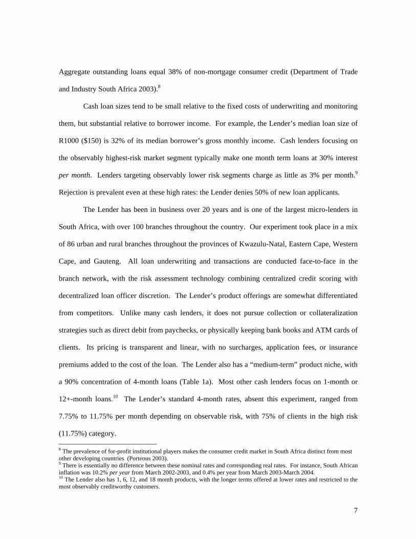
Aggregate outstanding loans equal 38% of non-mortgage consumer credit (Department of Trade
and Industry South Africa 2003).8
Cash loan sizes tend to be small relative to the fixed costs of underwriting and monitoring
them, but substantial relative to borrower income. For example, the Lender’s median loan size of
R1000 ($150) is 32% of its median borrower’s gross monthly income. Cash lenders focusing on
the observably highest-risk market segment typically make one month term loans at 30% interest
per month. Lenders targeting observably lower risk segments charge as little as 3% per month.9
Rejection is prevalent even at these high rates: the Lender denies 50% of new loan applicants.
The Lender has been in business over 20 years and is one of the largest micro-lenders in
South Africa, with over 100 branches throughout the country. Our experiment took place in a mix
of 86 urban and rural branches throughout the provinces of Kwazulu-Natal, Eastern Cape, Western
Cape, and Gauteng. All loan underwriting and transactions are conducted face-to-face in the
branch network, with the risk assessment technology combining centralized credit scoring with
decentralized loan officer discretion. The Lender’s product offerings are somewhat differentiated
from competitors. Unlike many cash lenders, it does not pursue collection or collateralization
strategies such as direct debit from paychecks, or physically keeping bank books and ATM cards of
clients. Its pricing is transparent and linear, with no surcharges, application fees, or insurance
premiums added to the cost of the loan. The Lender also has a “medium-term” product niche, with
a 90% concentration of 4-month loans (Table 1a). Most other cash lenders focus on 1-month or
12+-month loans.10 The Lender’s standard 4-month rates, absent this experiment, ranged from
7.75% to 11.75% per month depending on observable risk, with 75% of clients in the high risk
(11.75%) category. 8 The prevalence of for-profit institutional players makes the consumer credit market in South Africa distinct from most other developing countries (Porteous 2003). 9 There is essentially no difference between these nominal rates and corresponding real rates. For instance, South African inflation was 10.2% per year from March 2002-2003, and 0.4% per year from March 2003-March 2004. 10 The Lender also has 1, 6, 12, and 18 month products, with the longer terms offered at lower rates and restricted to the most observably creditworthy customers.

8
Borrowers face several incentives to repay these high-interest loans. Carrots include
decreasing prices and increasing future loan sizes following good repayment behavior. Sticks
include reporting to credit bureaus, frequent phone calls from collection agents, court summons,
and wage garnishments.
III. Experimental Design and Implementation
We identify specific types of asymmetric information by integrating the random
assignment of interest rates into the day-to-day operations of a consumer lender. This section
outlines the experimental design and implementation, describes related data collection, and
validates the integrity of the random assignments using several statistical tests. The methodology
is implemented in a consumer credit market, but is applicable to other market settings as well.
The experiment was pilot-tested in July 2003, and then fully executed in two additional
waves launched in September and October 2003. We begin with a brief overview of the
experiment, and then describe each step in detail below.
A. Design Overview
First the Lender randomized interest rates attached to “pre-qualified,” limited-time offers
that were mailed to 57,533 former clients with good repayment histories.11 Two rates were
assigned to each client: an “offer rate” (ro) included in the direct mail solicitation, and a “contract
rate” (rc) that was weakly less than the offer rate and revealed only after the borrower had accepted
the solicitation and applied for a loan. Clients did not know beforehand that the contract rate may
be lower than the offer rate. For 59% of the clients, the contract rate was identical to the offer rate.
11 Private information may be less prevalent among past clients than new clients if hidden information is revealed through the lending relationship (Elyasiani and Goldberg 2004). Hence, if this experiment were conducted on individuals with no prior borrowing history, one may expect larger information asymmetries. To estimate the information asymmetries on such individuals, we also sent soliciations to 3,000 individuals from a mailing list purchased from a consumer database, but only 1 person from this list borrowed. A subsequent list was purchased and 5,000 letters sent (but without randomized interest rates) and only 2 people responded. We return to this issue in Section VI.

9
Final credit approval (i.e., the Lender’s decision on whether to offer a loan after updating the
client’s information) and the loan size and term offered to the client were orthogonal to the
experimental interest rates by construction. Therefore the two interest rate randomizations enable
us to cleanly distinguish selection effects from repayment burden effects, since some clients will
select on different interest rates ex-ante, but then have identical repayment burdens ex-post, while
other clients will select on the same rate ex-ante, but have different repayment burdens ex-post. 12
We also randomly assigned differential dynamic repayment incentives (D) in order to
cleanly identify the moral hazard component of any repayment burden effects. Some clients were
assigned eligibility to receive rc on all future loans taken within the next year (D=1), conditional on
repayment performance, while others obtained rc for just the first loan (D=0). D=1 provides
favorable pricing on future borrowing (in the 98% of cases where rc was less than the Lender’s
standard rate) but does not shift the cost of repaying the borrower’s initial loan taken at rc. Thus D
enables us to test whether a marginal incentive, access to future financing at preferable rates,
induces better choices related to repayment; i.e., whether D reduces any moral hazard found in this
market. Clients were informed of D by the branch manager after all paperwork had been
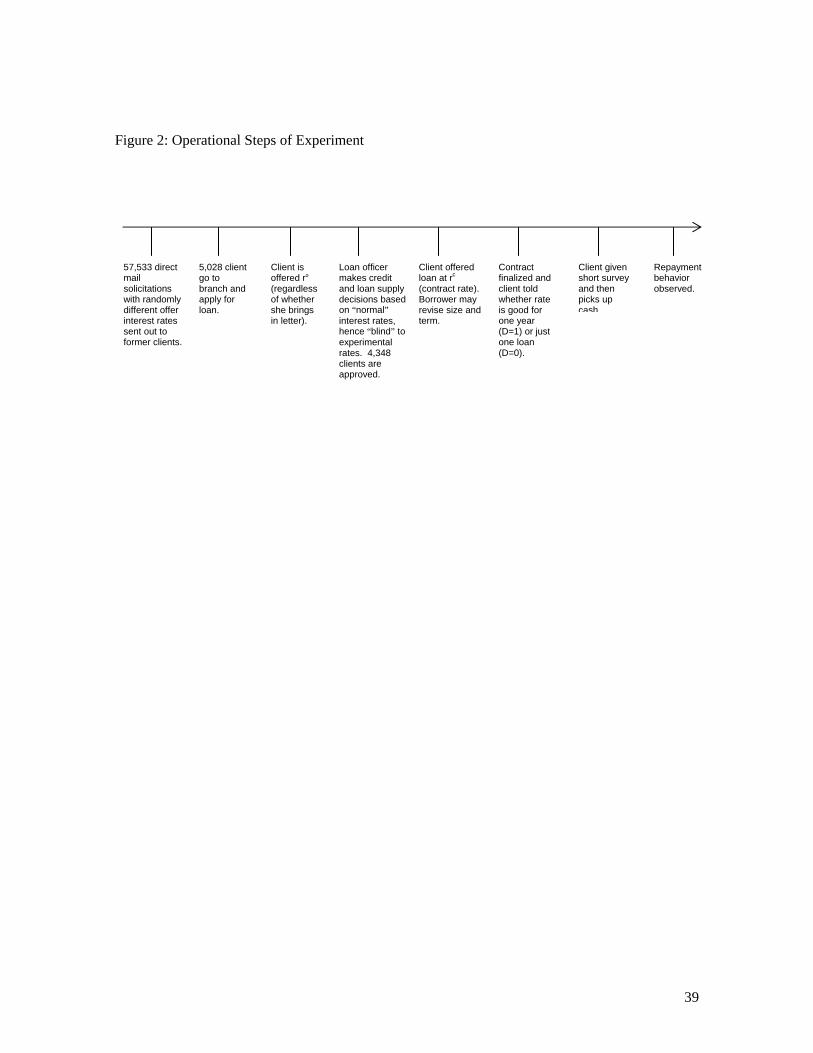
completed and all other terms of the loan were finalized. Figure 2 shows the experimental
operations, step-by-step. Figure 3 shows a scatter plot of the offer rate against the contract rate for
all individuals (41% of sample) who were assigned rc < ro.
B. Sample Frame
The sample frame consisted of all individuals from 86 branches who had borrowed from
the Lender within the past 24 months, were in good standing, and did not have a loan outstanding
in the thirty days prior to the mailer. Tables 1a and 1b present summary statistics on the sample
frame and the sub-sample of clients who obtained a loan at rc by applying before the deadline on 12 As detailed in Section IV, we define “repayment burden” as the reduced-form combination of several underlying moral hazard parameters and a wealth effect.

10
their mailer. Most notably, clients differ in observable risk as assessed by the Lender. The Lender
assigns prior borrowers into “low”, “medium”, and “high” risk categories, and this determines the
borrower’s loan pricing and term options under normal operations. The Lender does not typically
ask clients why they seek a loan, but the experimental protocol included a survey that indicates the
following self-reported uses: education (19%), housing renovations (11%), payoff other debt
(11%), household consumption and/or family event (13%), funeral and medical (4%) and
miscellaneous/unreported (32%).
C. The Randomizations
Each client was assigned three random variables: an offer interest rate (ro), a contract
interest rate (rc), and a binary variable for whether the contract rate would be valid for up to one
year (D=1) or one loan (D=0). Rates varied from 3.25 percent per month to 11.75 percent per
month.13 41% of the sample was chosen randomly and unconditionally to receive rc<ro (Table 1a).
At the time of the randomization, we verified that the assigned rates were uncorrelated with other
known information, such as credit report score. Table 2 shows that the randomizations were
successful, ex-ante, in this fashion, i.e., conditional on the observable risk category, ro and rc were
uncorrelated with other observable characteristics.14
Lastly, each individual was assigned to receive rc either for one full year (D=1) or for only
the first loan (D=0). In the pilot and the second wave of the experiment, this randomization was
13 Appendix Table 1 shows the resulting ro and rc distributions conditional on the three observable risk categories. Note these are “add-on” rates, where interest is charged upfront over the original principal balance, rather than over the declining balance. We adopt the cash loan market’s convention of presenting rates in add-on, monthly form. 14 Column 3 shows that the dynamic repayment incentive was predicted by number of months since the last loan, the number of prior loans and age. However, including a control for this in the primary specifications do not change the estimates of the effect of the dynamic incentive on default.

11
conducted at the branch level, such that 14 branches were assigned D=0, and 10 branches were
assigned D=1. In the third wave, this randomization was done at the individual level.15
D. The Offer and Loan Application Process
The Lender mailed solicitations featuring the offer rate to 57,533 former clients. Each
letter had a deadline by which the individual had to respond in order to obtain ro. The deadline
ranged from 2 weeks to 6 weeks, and is discussed in related research (Bertrand, Karlan,
Mullainathan, Shafir and Zinman 2004).16 The Lender routinely mails teasers to former borrowers
but had never promoted specific interest rate offers before this experiment.
Clients accepted the offer by entering a branch office and filling out an application in
person with a loan officer. Loan applications were taken and assessed as per the Lender’s normal
underwriting procedures. Specifically, loan officers: a) updated observable information and
decided whether to offer any loan based on their updated risk assessment; b) decided the maximum
loan size for which applicants qualified; and c) decided the longest loan term for which applicants
qualified. Each decision was made “blind” to the experimental rates. Table 2 Column 5 verifies
that the Lender’s rejection decision was in fact uncorrelated with the contract interest rate and
dynamic repayment incentive. 5,028 (8.7%) clients applied for a loan under this experiment, and
of those 4,348 (86.5%) were approved.
In determining maximum loan size, the Lender relies on a debt service ratio: the monthly
payment of a loan may not exceed a certain percentage of their net monthly income. A lower
interest rate would thus allow for a larger loan. A larger loan might then generate a repayment
burden effect, which could cause a higher default rate (and bias against finding moral hazard with
15 The dynamic repayment incentive randomization was done initially at the branch level because operations personnel at the Lender were concerned that it would be complicated to communicate D on a case-by-case basis. Once the branches were more comfortable with the experimental design, this was relaxed for the third (and largest) wave of offers. 16 The solicitations also incorporated randomized decision frames and cues, inspired by findings from marketing and psychology literatures, that were designed to estimate the impact of these “behavioral” effects on consumer demand. These randomizations were orthogonal to the pricing randomizations examined here, by construction.

12
respect to the interest rate). In order to mitigate this potential confound, the maximum allowable
loan size was established based on the normal, not experimental, interest rates.
The contract rate rc was kept secret from both the loan officer and borrower until after the
officer approved the loan application and a loan amount and term were established.17 Special
operations software was developed to facilitate and control this process, and we verify that this
condition held in practice in Table 2, column 4 by testing that the offer rate, and not the contract
rate (once controlling for the offer rate), predict take-up of the loan. Once the other loan contract
features were agreed upon, the software then revealed rc, which was weakly less than ro. If the
rates were the same, no mention was made of the second rate. If rc<ro, the loan officer told the
client that the actual interest rate was in fact lower than the initial offer. Loan officers were
instructed to present this as simply what the computer dictated, not as part of a special promotion
or anything particular to the client.
Clients then were permitted to adjust their desired loan size L following the revelation of
rc. In theory endogenizing L in this fashion has implications for identifying moral hazard effects
(since a lower rc strengthens repayment incentives ceterus paribus, but might induce choice of a
higher L that weakens repayment incentives), as discussed below. But in practice only 10% of
borrowers changed their loan demand after rc was revealed (Karlan and Zinman 2004).18
Finally, the software informed the loan officer whether the individual’s rc was valid for one
year (47% of borrowers obtained D=1) or for one loan (53% obtained D=0).
17 There are several reasons to implement the contract rate assignment “double-blind”. Most importantly, we did not want the contract rate to contaminate any selection effects (by influencing either credit approval, or the applicant’s decision whether to accept the loan offer). The double blind device also elicits two points on the credit demand curve for each consumer who received rc<ro (Karlan and Zinman 2004). 18 On the other hand, project clients did exhibit significant interest rate elasticities with respect to ro on both the extensive and intensive margins (Karlan and Zinman 2004).

13
E. Default Outcomes
We use three measures of default: (1) Monthly Average Proportion Past Due (the average
default amount in each month divided by the total debt burden), (2) Proportion of Months in
Arrears (the number of months with positive arrearage divided by the number of months in which
the loan was outstanding), and (3) Account in Collection Status (typically, the Lender considers a
loan in collection status if there are three or more months of payments in arrears). Table 1a
presents the summary statistics on the default measures. These measures were chosen in
consultation with the Lender as proxies for the credit risk, collection costs, and ultimate bad debt
incurred by the firm.
IV. Theoretical Overview
We begin by discussing the specific models of private information that motivate our
experimental setup, and then describe how the experimental design maps into these models. The
Theory Appendix provides a more formal derivation.
We test across two models of selection on unobservables: the Stiglitz-Weiss (1981)
adverse selection model (hereafter “SW”) and the de Meza and Webb (1987; 2001) advantageous
selection model (hereafter “DW”).19 Specifically, ro can produce either adverse or advantageous
selection, depending on the relationship between borrower risk and return.20 If risk, defined from
the Lender’s perspective as the probability of default, and borrower returns are positively
correlated, then SW implies that higher rates induce unobservably less risky borrowers to drop out
of the applicant pool. Thus under adverse selection, repayment would decrease in ro as we move 19Klonner and Rai (2004) provides a clear comparison of the Stiglitz-Weiss and de Meza-Webb models of selection. 20There is potentially a third type of selection based on private information, a “lemons” effect, which is unlikely to be important in our setting. As described in Ausubel (1991) and elsewhere, given a setting with competitive bargaining and the presence of private information generated from lending relationships, a single deviating lender would find that reducing rates attracts ex-ante unobservably worse repayment risks, since competing lenders will match the rate reduction only for the better risks. But survey evidence on pricing practices in the cash loan market suggests strongly that lenders as a rule do not make price concessions, even for good customers. Note that while the lemons effect is commonly described as adverse selection, in our setting it is analogous to advantageous selection in the sense that reducing interest rates decreases profitability on the margin.

14
away from the initial equilibrium. If risk and return are negatively correlated, then DW implies
that higher rates induce unobservably riskier borrowers to drop out of the applicant pool. Thus
under advantageous selection, repayment would increase in ro as we move away from
equilibrium.21 In a consumer credit context, this would hold if borrowers with unobservably
relatively unstable income view high interest rates as unaffordable. One limitation of our setup is
that if there are heterogeneous selection effects, such that some borrowers select adversely and
others advantageously, then the effect of ro will obscure the true magnitude of selection on
unobservables. We explore this in Section VI, although empirically, we cannot distinguish
heterogenous intensity of adverse selection from offsetting adverse and advantageous effects.
The second randomly assigned interest rate, rc, identifies the impact of repayment burden
via a combination of several underlying structural parameters of interest. Repayment burden
incentives operate through the borrower’s project management and repayment choices. Project
management choices are defined as those that impact returns. Higher interest rates will produce
moral hazard in project choice (conditional on effort) if borrowers prefer mean-preserving spreads
in project returns under limited liability (Stiglitz and Weiss 1981). Similarly, higher interest rates
reduce effort (conditional on project choice), by producing debt overhang that reduces borrower
returns in successful states (Ghosh, Mookherjee and Ray 2000). Repayment choice simply refers
to the fact that voluntary default (conditional on project returns) becomes more attractive under
limited enforcement as repayment burden increases (Eaton and Gersovitz 1981; Ghosh and Ray
2001). In contrast, the income effect of repayment burden has nothing to do with choice: it works
mechanically, by simply increasing the probability that a borrower with uncertain cash flow will be
unable to repay. Note that each of these hypothesized incentive and income effects works in the
same direction — a higher repayment burden decreases the probability of repayment.
21 de Meza and Webb (2000) shows that advantageous selection can persist in equilibrium if moral hazard prevents lenders from raising interest rates to clear the market.

15
These four components of repayment burden all have intuitive salience in this setting, and
hence our priors are agnostic regarding their relative importance. Project choice may be relatively
limited (compared to say a pure commercial loan market), or may not — anecdotal reports suggest
the possibility of “hidden” investment in entrepreneurial projects, and survey evidence reveals
cross-sectional variation in the deployment of funds consistent with a range of consumption
smoothing and human capital investment opportunities. Debt overhang might also be less salient
in a consumer rather than commercial credit setting, but then again the relevant effort in the
consumer case might be related to maintaining one’s wage employment, or to obtaining credit from
the informal sector in the event of a negative outcome. Voluntary default might be mitigated by
reputation effects (repeat contracting opportunities) and aggressive (if imperfect) enforcement, but
to what extent? The size of the income effect depends critically on the variance of borrower cash
flows, which we do not observe.
V. Empirical Strategy
We now present the empirical strategy used to test the theoretical models and interpret the
results of the experiment. Recall that we identify any selection and repayment burden effects by
randomly assigning separate offer and contract interest rates to borrowers, conditional on
observable risk, and then estimating the relationship between loan repayment and these rates. We
employ five approaches to analyzing the results: stylized comparison of means, a base-case OLS
specification, a non-parametric matching estimator, and instrumental variables.
Abstracting from functional form considerations for the moment, our basic empirical
model takes the form:
(1) Yi = f(rio, ri
c, Di, Xi)

16
where i indexes borrowers. Y is a measure of repayment; ro is the rate offered on the mail
solicitation; and rc ≤ ro is the rate actually contracted upon loan approval. D is the randomly
dynamic repayment incentive (or lack thereof), with D=1 if rc is valid for up to one year (if the
borrower stays current), and D=0 if rc applies to one loan only. X always includes the Lender’s
summary measure of observable risk (since the interest rates were randomized conditional on this
measure), and also may include other readily observable characteristics that the Lender could use
for screening.
The Theory Appendix shows formally that:
• ro identifies the selection effect conditional on rc -- with dY/dro>0 if there is adverse
selection on net, and dY/dro<0 if there is advantageous selection on net.
• rc identifies the repayment burden effect conditional on ro — with dY/drc>0 if there is such
an effect.
Stylized Comparison of Means: Table 3
We classify rates into “high” and “low” groups, a la Figure 1. This is done by setting
cutoffs at the median experimental rates for each observable risk category. Table 3 presents mean
comparisons using this method. The findings preview the regression results: we find occasional
evidence of adverse selection and repayment burden in the full sample, and more robust evidence
for adverse selection among female borrowers and repayment burden among male borrowers.
OLS Specification: Tables 4 and 5
Our base specification is a linear model estimated using OLS:
(2) Yi = α + βorio + βcri
c + βwDi + χXi + εib

17
i again indexes borrowers, and βo, βc, and βw are the estimates of the selection effect, the repayment
burden effect, and the dynamic incentive effect, respectively. X need include only the Lender’s
summary measure of observable risk since the randomizations conditioned only on this variable.
We also include fixed effects for the month in which the offer letter was sent (June, September, or
October 2003). The error term, εib, is corrected for clustering at the branch level, b. The model is
estimated on the takeup sample of 4,348 observations since these are the only project clients for
whom we observe repayment behavior. The OLS results are robust to including loan size and term
as control variables, which is noteworthy since loan size responds to the interest rate (Karlan and
Zinman 2004) and could have an independent effect on default. Results obtained with the OLS
estimator are similar to the comparison of means, and are presented in Tables 4 and 5 and
discussed in Section VI.
Semi-Parametric Matching Estimator: Table 6
Next we develop a semi-parametric approach that resembles a matching estimator, but with
a continuous treatment variable. This is motivated by the concern that the OLS specification will
impose incorrect functional form assumptions if any of the three different random variables interact
to influence default. We address this possibility using three related specifications that impose a
functional form assumptions on only one random variable at a time, while conditioning non-
parametrically on all combinations of the other two random variables and observable risk. For
example, to identify the selection effect (ro), we group observations that match perfectly on the
other random variables (rc and D) and the risk level, and employ a fixed effect model that de-means
the dependent variable (default) and the variable of interest (in this case ro) within these perfectly-
matched groups. This model is shown is equation (3) below, and then we present the analogous
models for identifying the repayment burden effect and dynamic incentive effect in equations (4)

18
and (5), respectively. In each of these formulas the subscript “c” represents contract interest rate,
“o” represents offer interest rate, “d” represents the dynamic incentive, and “r” represents the
lender-defined categorical risk level (high, medium or low). The unit of observation is i, the
individual borrower. The month of the offer letter, M, is a categorical variable (either July,
September or October, 2003).
Match on c,d,r to identify the offer rate effect: (3) cdricdrio
cdro
icdrcdricdr MrrYY εεδβ −++−=− )(
Match on o,d,r to identify the contract rate effect: (4) odriodric
odrc
iodrodriodr MrrYY εεδβ −++−=− )(
Match on c,o,r to identify the dynamic incentive effect: (5) coricoricoricorcoricor MWWYY εεδβ −++−=− )(
Table 6 presents the estimates obtained using these three specifications. The results are discussed
in Section VI.
Instrumental Variables Estimator: Table 7
Lastly, we consider the case where repayment burden is defined as total interest due on the
loan, not merely the marginal cost of debt (the interest rate). Total interest due includes an
endogenous component (loan size) multiplied by a random variable (the interest rate), so we
employ an instrumental variables approach to identify the effect of loan pricing on default.
Specifically, we use the random variables to instrument for endogeneous variable of interest, debt
burden. The instrumental variable specification is:
(6) iicic
oii XIIY εδββα ++++= ˆˆ
0
where I0 and IC are the endogenous variables, total interest due under the offer and contract
rates, respectively. The first stage specifications are:
(7) Iio = α1 + β1
orio + β1
cric + χ1Xi + υ1
i
and

19
(8) Iic = α2 + β2
orio + β2
cric + χ2Xi + υ2
i
with rio and ri
c serving as instrumental variables.
These results are presented in Table 7 and discussed in the next section.
Plot of Coefficients: Figures 4-11
In figures 4-11 we relax the linear treatment effect assumptions imposed by (2)-(8) using a
nonparametric graphical approach described in Section VI, part D.
VI. Empirical Results
A. Overview of Base Specification
Our primary analysis estimates equation (2) using ordinary least squares, tobit, or probit on
the “full” sample containing all three observable risk categories (Table 4).22 The dependent
variables are the three default measures described above. In all specifications, the interest rate
units are in monthly percentage points (e.g., 7.50 for 7.50% per month), and we report marginal
effects where applicable. Results on interest rate variables therefore capture the effect of a one
percentage point (100 basis point) increase in the monthly rate. We find evidence of moral hazard
through the dynamic pricing incentive D, but little suggestion of any selection on unobservables in
the full sample.
22 Results are robust to including the log of loan size, and loan term, to address the possibility of interest rate effecting repayment through its effect on loan size and term. An alternative, instrumental variables approach is presented in Table 7. This too yields qualitatively similar results. Nor do results change if we include branch fixed effects to control for any differences in experimental implementation and/or the mechanical influence of varying mailer dates (staggered by groups of branches) on repayment measures. Pooling the risk categories implies that the full sample model lacks a common support for interest rates exceeding 7.75 (since, e.g., low risk borrowers are never offered a rate above 7.75). We re-estimate our base specifications over a common support and report qualitatively similar results in Appendix Table 2, although much power is lost on the smaller sample size.

20
B. Primary Results with the Base Specfication Row 1 of Table 4 presents estimates of βo, the response of repayment behavior to the offer
rate. This coefficient identifies any net selection on unobservables, with βo>0 indicating adverse
selection, and βo<0 indicating advantageous selection. We find no robust evidence in either
direction on the full sample.23
Row 2 of Table 4 presents estimates of βc, the response of repayment behavior to the
contract rate. This coefficient identifies any effect of repayment burden, with βc>0 indicating some
combination of moral hazard and wealth effects. Similar to the adverse selection results, we find
consistently positive effects that are typically insignificant statistically. The one marginally
significant result (column 2) implies that a 400 basis point cut would reduce the average number of
months in arrears by 13%.24
Results on D, the dynamic repayment incentive variable, deliver robust evidence of moral
hazard (Table 4, row 3). Recall that clients with D=1 face a marginal incentive to repay — if they
maintain good standing with the Lender they are eligible to borrow at rc for up to a year. D
consequently has no effect on the debt burden of the current loan, but does increase the benefit of
maintaining a good relationship with the lender by reducing the interest rate on future loans. D
therefore is free of the noise (bad shocks) and confound (endogenous loan size) that might bias
estimates of the reduced-form repayment burden effect toward zero. D thus identifies pure moral
hazard that is alleviated by the provision of a marginal, dynamic repayment incentive. D’s effect is
large and significant, with the incentive producing decreases in the various default measures
23 Recall from Section IV that the offer rate coefficient will understate the true extent of private information problems if there are concurrent adverse and advantegeous selection effects in the sample. This would manifest as parameter heterogeneity; e.g., if part of the sample has βo<0, and part of the sample has βo>0. We explored this possibility by interacting the offer rate variable with various demographics (see, e.g., Table 8), and found some evidence that adverse selection was decreasing in income. Splitting the sample into income quintiles or at the median (not reported), we found that only one of the six offer rate coefficients had the negative sign consistent with advantageous selection, and that this coefficient was not statistically significant (t-stat = 0.6). 24 Coefficient * 4 / mean outcome = 0.007 * 4 / 0.219 = 13%

21
ranging from 1.1 to 1.9 percentage points in the OLS specifications on the full sample. These
magnitudes imply that D=1 clients defaulted 7 to 16 percent less often than the mean borrower.
Table 4 (Columns 2, 4 & 6) also shows that this effect is increasing in and driven by the size of the
discount on future loans, as each 100 basis point decrease in the price of future loans reduces
default by 4% in the full sample.
Table 5 shows the primary results from Table 4, but by gender. We find significant and
robust evidence of moral hazard (but not adverse selection) for males, and adverse selection (but
not moral hazard) for females. The issue of differential response to interest rates by gender is of
particular interest to development economists and microfinance practitioners, given that
microcredit initiatives often target women, in part because females are considered more likely to
repay loans and/or less able to obtain formal sector credit.25
Table 5, Columns 1 through 6 show the results for male borrowers. We find evidence of
moral hazard but no selection on unobservables. Both experimental instruments for moral hazard,
the contract rate and the dynamic repayment incentive (D), are large and sometimes significant
determinants of default. The coefficient on the offer rate is relatively small and always
insignificant.
Table 5, Columns 7 through 12 show a different pattern for female borrowers. We find
evidence of adverse selection but no repayment burden or moral hazard effects. The offer rate
coefficient is always large and positive for females, and statistically significant in 5 of the 6
regressions reported, indicating adverse selection. On the other hand, the contract rate coefficient
is now wrong-signed (and significant in one case). The dynamic repayment incentive results are
insignificant, but signed negatively (evidence for moral hazard) and often large economically. On
25 Although the reasons for this are unclear, anecdotal evidence suggests that women are weakly more likely to repay microcredit loans. Studies of consumer choice in other financial markets have found gender differences. Barber and Odean (2001) finds that males are more likely to trade excessively in public equities. Pitt and Khandker (1998) finds that impacts of participation in a mircofinance program differ by gender.

22
balance then there is no statistically significant evidence for repayment burden or moral hazard
influencing the repayment behavior of female borrowers.
In specifications not shown, we test whether the gender effects are significantly different
from each other by including gender interaction terms in the Table 4 specifications. The
interaction term is significant statistically for both the offer and contract interest rates, but not for
the dynamic repayment incentive variable. This is not surprising, since the coefficient on the
dynamic repayment incentive for women is negative and similar (slightly smaller) to that for men,
just not significant statistically.
C. Primary Results with Matching Estimator and IV Specification
Table 6 presents the results of the semi-parametric matching estimator specified in
equations (3)-(5). The point estimates remain largely the same as in the OLS results shown in
Table 5, but the standard errors are slightly larger due to the loss of hundreds of degrees of
freedom.
Table 7 presents the results of the IV estimator outlined in equations (6)-(8). These follow
a similar pattern to the results obtained from the base specification (Tables 4 and 5), with the
exception that we now find more weakly significant evidence for adverse selection. (As before,
however, the significant full sample results appear to be driven by females.) Results from
estimating the endogenous version of the IV estimator (second panel of Table 7) suggest that using
total interest cost (or debt burden) as the regressor can lead to misleading inferences in cases where
exogenous variation is not available. We surmise that the difficulty stems from the fact that lower
interest rates-- i.e, a lower marginal cost of borrowing-- produce demand for larger loan sizes
(Karlan and Zinman 2005), and hence a larger total cost of borrowing. Recall that our IV estimator

23
surmounts this problem by instrumenting for the total cost of borrowing with our randomly
assigned marginal cost of borrowing.
D. Graphs
Figures 4-11 show smoothed plots of coefficients from a non-parametric estimator that
relaxes the linear treatement effect assumption maintained in all of our regression specifications.
Each plot has one random variable of interest; e.g., in Figure 4 this variable is the offer rate. The
estimates of interest are the coefficients on the each individual offer rate (e.g., one cell for 7.25,
another for 7.5). The specifications include controls (again, non-parametric) for the contract
interest rate, risk category and month of the offer. The plots reproduce the qualitative patterns
(sign and magnitudes) found in our regressions, but are not conclusive in the sense that the
confidence intervals leave open the possibility of nontrivial nonlinearities.26
E. Gender Analysis
Next, we explore whether the gender effects are actually driven by systematic variation in
household demographics rather than something unobservable and/or fundamental to gender per se.
Tables 1a and 1b show that there are minimal compositional differences across gender. A
parsimonious test (shown in Table 8) for compositional confounds is to add interactions between
the interest rate variables and observable characteristics to our base specification. The significant
interaction terms between gender and the rate variables, conditional on other demographics (and
their interactions with rates and gender), suggest that gender differences are not merely driven by
mechanical composition effects. We continue to find strong repayment burden effects among
males, and strong adverse selection effects among females. None of the demographic interaction
effects are significant, nor do they detract from the simple gender interaction effects with rates. If, 26 The confidence bands on these plots were created by bootstrapping with 500 replications.

24
for instance, the gender effect was masking a “female and married” effect, then we would observe a
significant “married and offer rate” interaction and the gender interaction with the offer rate would
go to zero.
A related check is to predict default using observable demographic information, and then
test whether observable selection on the interest rate differs across males and females. If
unobservably riskier women are more likely to borrow at high interest rates, one should also find
that observable riskier women are also more likely to borrow at high interest rates. Table 9 shows
these results: specifically, the effect of the interaction between observable risk and the offer rate on
the decision to apply is significant and positive for women, but not for men. This means that the
price elasticity of the application decision is decreasing in observable risk for women but not for
men, and provides further confirmation of a gender difference that is not driven purely by other
observable characteristics.
Of course we do not observe all of the observable characteristics of interest; e.g., we do not
have independent measures of education and occupation, nor do we observe health status,
unmarried co-habitation or head-of-household. Hence the above tests do not completely rule out
the possibility that relatively mechanical demographic differences generate the observed gender
pattern.
On balance, however, the evidence suggests that male and female borrowers do pose
different types of private information problems for the Lender, with strong evidence that females
select adversely and some evidence that male repayment is sensitive to repayment burden. The
question of what drives this pattern (e.g., demographics, outside credit options, social norms, hard-
wiring....) merits further, more systematic, exploration.

25
F. Observable Determinants of Default and Selection on Observables
Significant interactions between interest rates and observable characteristics beg the related
question of how efficiently the Lender assesses risk. We begin by exploring whether observable
characteristics help predict default, conditional on the Lender’s summary statistic for risk, by
reporting results obtained from adding several additional observables to equation (2). Table 10
shows that the Lender’s summary statistic for observable risk does not in fact completely
summarize the role of observables, at least over the range of interest rates used in our experiment.
Each specification includes an indicator variable for the sufficient statistic the lender uses (one of
11 categories) in their risk assessment. Regardless of specification, several readily observed
variables help predict default, including credit scores and the number of prior transactions with the
Lender. However, adding observables beyond the summary statistic generates little or no
improvements in the overall explanatory power of the models (as measured by the adjusted R-
squareds in Tables 4 and 10).
G. External Validity and the Power of Repeated Transactions
We may find little evidence of adverse selection in the full sample because our borrowers
have already revealed their types to the Lender; i.e., in the process of transacting, private
information becomes public.27 We explore this possibility indirectly, and within-sample, by
exploring whether the offer rate effect varies with the number of prior loans the borrower has taken
from the Lender. Table 11 shows that this is indeed the case: adding a prior loans main effect and
interaction with ro to equation (2) produces a negative and significant interaction term. The
interaction effect is large; e.g., it eliminates 43% of adverse selection at the mean number of prior
27 We sought to include clients with no prior relationship with the Lender by extending 3,000 offers to names obtained from a mailing list; unfortunately, the list results in one borrower. A pilot follow-up list of 5,000 offers (without randomization of interest rates) yielded two borrowers. Hence, in order to conduct this experiment on “new” clients, we need to find an alternative channel for identifying the sample frame and contact information.

26
loans (4.3) in the full sample. Thus selection is indeed relatively more adverse for those borrowers
with whom the Lender is least familiar. The repayment burden effect (through the contract interest
rate) appears to decrease with prior transaction frequency as well. Moral hazard (as identified by
the dynamic repayment incentive), on the other hand, abates only a little. Note, however, that we
should not conclude that the relationship caused the information asymmetries to abate. Rather, if
those with more frequent transaction histories are simply less able or willing to exploit information
asymmetries, then we also would find negative coefficients on the interactions between interest rate
and prior borrowing frequency. In other words, we can not distinguish whether it is the frequent
borrowers’ “type” or the relationship itself that drives the results. Think of implementing our
experiment on the most frequent borrowers, but years ago, before their first loan with the Lender.
If their “type” is driving today’s behavior, then this initial experiment also would have found no
evidence of adverse selection or moral hazard. Repeated experiments, and panel data, would help
identify the causal effects of lending relationships.
H. Magnitude Calculations Comparing Observables and Unobservable Effects
We now estimate the relative importance of private vs. public information in determining
default. Recall that the Lender uses the three-tiered risk category to determine interest rates. High
risk clients typically have much higher default rates; e.g., a 20 percentage point higher proportion
of months in arrears than low risk clients (27 percentage points for men, and 17 percentage points
for women).28 We take this observable difference and calculate how much of it appears to be due
to information asymmetries with respect to interest rates. Recall that low risk borrowers typically
pay 400 basis points less per month than high risk borrowers. The point estimates suggest that this
28 In our sample, there is a 22 percentage point difference in default between high and low risks among borrowers who obtained rates within 100 basis points of the Lender’s normal rate for their risk class. The unadjusted mean difference in our sample is 15.0 percentage points (Table 1a).
27
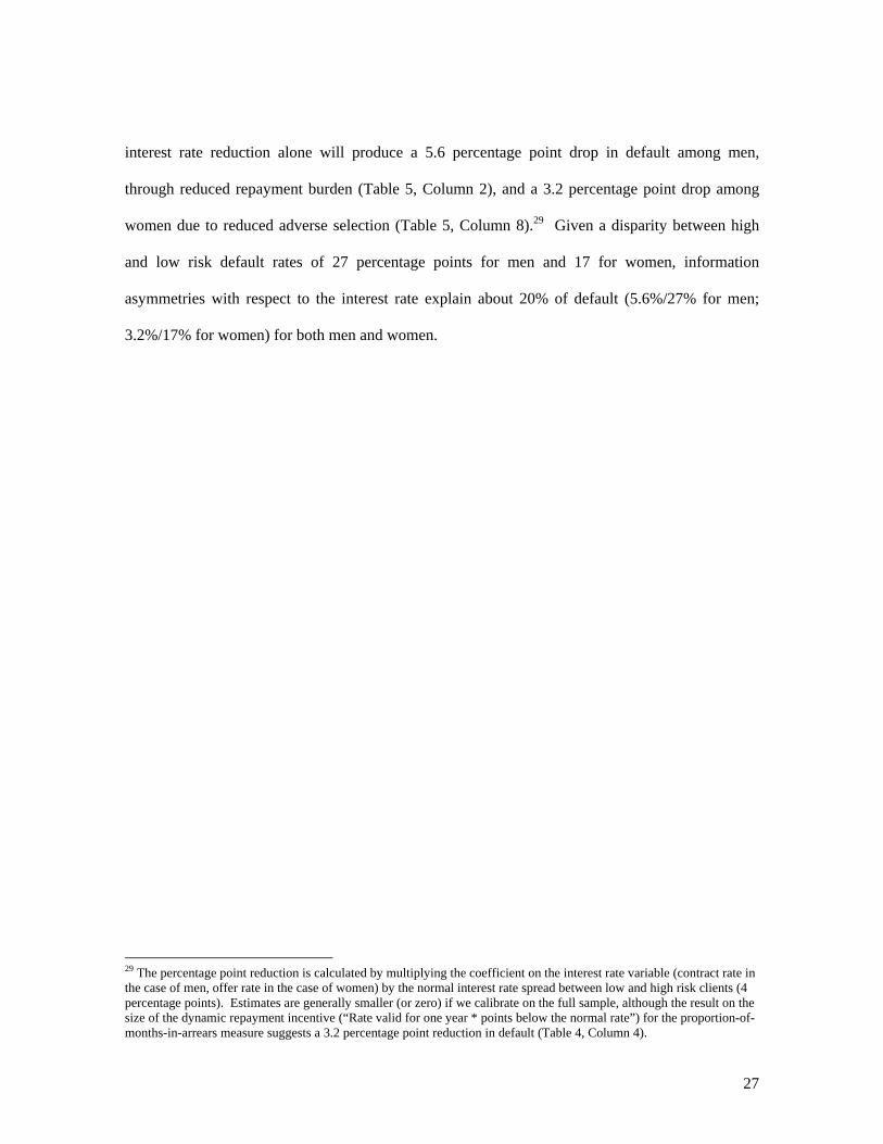
interest rate reduction alone will produce a 5.6 percentage point drop in default among men,
through reduced repayment burden (Table 5, Column 2), and a 3.2 percentage point drop among
women due to reduced adverse selection (Table 5, Column 8).29 Given a disparity between high
and low risk default rates of 27 percentage points for men and 17 for women, information
asymmetries with respect to the interest rate explain about 20% of default (5.6%/27% for men;
3.2%/17% for women) for both men and women.
29 The percentage point reduction is calculated by multiplying the coefficient on the interest rate variable (contract rate in the case of men, offer rate in the case of women) by the normal interest rate spread between low and high risk clients (4 percentage points). Estimates are generally smaller (or zero) if we calibrate on the full sample, although the result on the size of the dynamic repayment incentive (“Rate valid for one year * points below the normal rate”) for the proportion-of-months-in-arrears measure suggests a 3.2 percentage point reduction in default (Table 4, Column 4).

28
VII. Conclusion
We develop a new market field experiment methodology that disentangles adverse selection from
moral hazard. The experiment is implemented in a South African consumer credit market, and
yields evidence of moral hazard among males and adverse selection among females. This confirms
the conventional wisdom on moral hazard in microfinance but raises a new puzzle for theorists and
practitioners: why do we only see adverse selection among women? In the full sample, these
findings aggregate to robust evidence for moral hazard and weak evidence for adverse selection.
The magnitudes of these information problems decrease with individuals with lengthier prior
lending relationships with the Lender. Where statistically significant, the effects of private
information are economically important: our results indicate that adverse selection and moral
hazard explain about 20% of default in our sample. Overall the findings provide unique empirical
evidence of significant, specific information asymmetries in a consumer credit market, and thus
help explain the prevalence of credit constraints even in a market that specializes in financing high-
risk borrowers at very high rates.
We are building on this work in several respects. The gender results motivate additional
experiments, in the lab and in the field, to test their robustness across different settings and unravel
any underlying drivers of the observed differences.30 The presence of significant information
problems provides a microfoundation for credit rationing, but not a sufficient condition for welfare-
enhancing interventions (no matter how well-run), as efficiency depends critically on borrower
returns. This helps motivate the next experiment with this Lender and others in the Philippines and
Brazil where we randomly provide credit to marginally rejected borrowers and follow-up with
household surveys to document loan uses and outcomes. This is another step in identifying the
30 The results also motivate additional data collection on, for example, the incidence of bad shocks by gender. In a brief phone survey, reaching 374 former borrowers of the Lender (including 61 defaulters), we found no differential incidence of adverse shocks.

29
existence, causes, and consequences of specific market failures via field experiment methodologies
that can be replicated, refined, and implemented in different countries and product markets.

30
Theory Appendix Here is a more formal derivation of how our research design maps into theoretical models of
private information, and thereby permits identification of unobservable selection and moral hazard
effects.
Assume a Lender implementing our experiment is faced with loan applicants who have identical
observable characteristics but may be heterogeneous with respect to unobservable information.
These characteristics q are not observable to the Lender, but are known to the applicant. Let q
(“riskiness”) be continuous, and bounded below by zero: )},0[,{ ∞∈= qqQ , where a higher q
negatively impacts but does not wholly determine the “success” of the borrower’s project, which is
defined discretely. The success/fail framework is most intuitive in a pure commercial credit
market, but also applies to a consumer credit setting. Here we can think of “success” as having
sufficient funds to repay the consumer cloan, whether these funds are from entrepreneurial activity,
wage income, or other financing sources, and we can think of q as about the inherent riskiness,
unobservable to the lender, of the consumer having such funds available to them ex-post to repay
the loan. Borrowers succeed with probability p(q, e) and fail with probability 1-p(q,e), where e is
effort exerted by the agent. We allow effort to be continuous, ]1,0[∈e , and assume it imposes a
linear cost.
We assume that p is twice continuously differentiable in effort, and differentiable with respect to
the common shock and the unobservable risk q. Next we impose the following standard
assumptions on the probability structure:

31
Assumption 1.
.0)1,(,)0,(:
.0),(,0),(,0),(,0),( 2
2
2
=∂
∂∞→
∂∂
<∂∂
∂<
∂∂
>∂
∂<
∂∂
eqp
eqpconditionsInada
qeeqp
eeqp
eeqp
qeqp
i.e., the probability of success decreases with riskiness, q; the probability of success increases with
borrower’s effort, e; and, the probability of success with respect to effort, e, decreases with
riskiness, q (and vica versa).
Next assume for simplicity that the return to the borrower is R(q) in the event of success and zero
in the event of failure. We assume for the moment that returns are observable and verifiable,
thereby abstracting from the possibility of voluntary default (Eaton and Gersovitz 1981; Ghosh and
Ray 2001). Then default occurs if and only if the project doesn’t succeed under the additional
simplifying assumption that:
Assumption 2. .)1()(: BrqRQq c+>∈∀
Where B is the loan principal amount demanded and rc is the interest rate on the loan contract. So
a borrower repays in full if her project succeeds and repays nothing if her project fails.
We now show that the assumption on the relationship between risk (to the Lender) and returns (to
the borrowers) is critical to identifying any selection effects of interest rates. Stiglitz and Weiss
(1981) shows that adverse selection results if this relationship is positive. Formally,
Assumption 3a (“SW”). ).()'(),'()(),(:', eCqReqpqReqpQqq ==∈∀

32
Where C is a constant. The equation states that expected returns to the borrower are constant—
projects that yield high returns in the successful state have low probabilities of success. We show
below that this condition will indeed produce adverse selection in our setting.
De Meza and Webb (1987) shows that advantageous selection results if risk and returns are
negatively correlated. Formally:
Assumption 3b (“DW”). ).'(),'()(),(':', qReqpqReqpqqQqq <⇔>∈∀
This will hold, e.g., if borrowers differ only in the probability of project success, but not in project
payoff conditional on success. We show below that in our setting 3b implies that raising the
interest rate discourages low quality borrowers on the margin, thereby improving the average
composition of the borrower pool via advantageous selection.
We solve for selection and moral hazard effects by focusing on the borrower’s problem. Define the
borrower’s expected return (after the effort choice is made) as:
eBrqReqpE c −+−= ])1()()[,()( )1( π
Where we assume that borrowers are price takers. We ignore the Lender’s problem since in our
setting the interest rate is not a choice variable, and the variables the Lender does control (loan

33
supply on the extensive and intensive margins) are orthogonal to the rate by construction.
Therefore we can assume (without loss of generality) that applicants are approved by the Lender.31
Accordingly we return to the borrower’s problem and begin by solving the model through
backwards induction; i.e., conditional on the borrower deciding to apply, she decides upon the
repayment effort after learning the contract interest rate, rc. Note the interest rate that the agent
takes into account is the contract rate, not the offer rate (in the case where they differ). Therefore,
holding riskiness, q, fixed, the agent solves
eBrqReqp c
e−+− ])1()()[,(max )2(
Given our set of assumptions, the optimization program yields a unique interior solution for each
value of q (and υ) and is characterized by the following first-order condition:
.)1()(
1)~,(:),(~ )3(BrqRe
eqprqee cc
+−=
∂∂
=
Proposition 1. The level of effort chosen is inferior to the first-best value (that is, when effort is
observable and verifiable). Moreover, note that .0/~ <∂∂ cre This is the debt overhang version of
moral hazard effect -- the higher the interest rate, the less the optimal effort since the agent only
receives a positive return in case of success (i.e., the return function is convex). Proof is at the end
of this Appendix. In this setup, a voluntary default model would yield qualitatively identical
results regarding the relationship between repayment and rc (Eaton and Gersovitz (1981) or Ghosh,
Mookherjee et al (2000)).
The next step in solving the borrower’s problem is to examine the decision to apply for the loan,
which is made using the offer rate, ro. (Recall from Section III that borrowers are not aware that
31 In practice, 84% of applicants were approved in the experiment. More generally, one can think of any rejected borrowers as being observably differentiated— and this model conditions on observable information.

34
there might be a distinct contract rate, rc, when they are deciding whether to apply for the loan.)
Define the marginal applicant as the one who has expected returns of exactly zero. That is,
.0)(])1()ˆ())[(,ˆ(:ˆ )4( =−+− ooo reBrqRreqpq
Proposition 2. If the SW assumption (3a) holds, the agent applies for a loan if .q̂q ≥ Moreover,
an infinitesimal increase in ro increases the marginal borrower’s q, .0/ˆ >∂∂ orq (There is no
effect through effort since it is endogenous, and the marginal effect is zero by the envelope
theorem). Therefore when the offer rate increases the marginal applicant is riskier; i.e., the safer
borrowers choose not to apply, creating a pool that is riskier on average. This is the classic adverse
selection effect a la SW. If instead the DW assumption (3b) holds, the agent applies if qq ~≤ . In
this case ,0/~ <∂∂ orq ; i.e., increasing the offer rate decreases the marginal applicant’s riskiness,
q, and the applicant pool becomes less risky on average. This is advantageous selection a la DW.
(See the end of this Appendix for proofs.)
We can now tie our propositions regarding the selection effects of the offer interest rate, ro, and the
moral hazard effect of the contract interest rate, rc, directly to an empirical outcome of interest, the
probability of default. According to the model, the expected probability of default, once rc is
known and effort is chosen, can be expressed as:
.)ˆ(1
)()]~,(1[default) of probabiliy( )5(ˆ∫∞
−−=
q qFdqqfeqpE
Proposition 3. The marginal effect of ro on the default probability captures the effect of selection.
If the SW assumption holds, then:

35
.0)],ˆ(1[)(1
)(ˆ)ˆ(1
)()],(1[)(1
)(ˆ)default ofy probabilit( )6(ˆ
>−−∂
∂−
−−
−∂∂
=∂
∂∫
∞eqp
qFqf
rq
qFdqqfeqp
qFqf
rq
rE
oqoo
The proof is a direct application of proposition 2. If instead the DW assumption holds then the
effect of a marginal change in the offer rate on the estimated probability of default has a negative
sign.
On the other hand the marginal effect of rc will capture the moral hazard effect,
.0)ˆ(1
)(~)~,()default ofy probabilit( )7(ˆ
>−∂
∂∂
∂−=
∂∂
∫∞
q cc qFdqqf
re
eeqp
rE
The result is again immediate since, by proposition 1, .0/~ <∂∂ cre
Incorporating the dynamic repayment incentive (D=1) is no different substantively than increasing
the benefits of repayment, holding the costs constant. This additional repayment incentive may
inspire more effort to ensure a successful outcome (debt overhang) or simply more incentive to
choose to repay the first loan (voluntary default. Incorporating this into the above, we add D to
formula 2 as a benefit which accrues to the borrower if they repay the first loan:
eBrDqReqp c
e−+−+ ])1()()[,(max )8(
.)1()(
1)~,(:),,(~ )9(BrDqRe
eqprDqee cc
+−+=
∂∂
=
.0/~ )10( >∂∂ De

36
Although not explicitly shown in the model, D is not merely binary, but rather is larger the lower rc
relative to the normal lender rate. The empirical strategy will analyze the incentive both as a
binary and as a continuous variable.
Proof of Proposition 1.
To show that the effort level is lower than the first-best level of effort, begin by noting that in a
first-best setting where effort is observable and verifiable to all parties the first-order condition
reads:
)(1),( *
qReeqp
=∂
∂
The right-hand side of this first-order condition is smaller than the one for which effort is
unobservable, making the optimal effort level larger due to decreasing returns in effort.
To show the moral hazard effect, ,0/~ <cdred totally differentiate the first-order condition to
obtain
[ ],0
)1(
~
2
2
2 <+−
∂∂
=BrR
ep
Bdr
edc
c
since the returns to effort are decreasing. Q.E.D.
Proof of Proposition 2.
Assume the SW assumption (3a) holds. Recall that the marginal borrower’s return once the offer
rate is announced is by definition. Since the expected returns are increasing in q only applicants

37
with q’s higher than marginal borrower’s q̂ are going to have nonnegative expected returns.
Accordingly these borrowers with qq ˆ> form the pool of applicants.
Totally differentiating the marginal applicant condition yields:
,0)~,ˆ,()1(
ˆ>
∂∂
+−=
qeqpBr
pBdr
qdo
o υ
since p is decreasing in unobservable risk q. If instead the DW assumption (3b) holds the steps are
the same but the signs are the opposite. In particular expected returns are decreasing in q and so
only safer projects than the marginal q apply. In this case the total differentiation produces:
[ ].0
)~,~()1(
~<
∂∂
+−=
qeqpBrR
pBdr
qdo
o Q.E.D.

38
Figure 1: Stylized Depiction of Experimental Design
N/ALow Offer Rate
High Offer Rate
Low Contract RateHigh Contract Rate
Moral Hazard / Repayment Burden
Adve
rse
Sele
ctio
n
N/ALow Offer Rate
High Offer Rate
Low Contract RateHigh Contract Rate
Moral Hazard / Repayment Burden
Adve
rse
Sele
ctio
n
39
Figure 2: Operational Steps of Experiment
Repayment behavior observed.
Client given short survey and then picks up cash
Contract finalized and client told whether rate is good for one year (D=1) or just one loan (D=0).
Client offered loan at rc (contract rate). Borrower may revise size and term.
Loan officer makes credit and loan supply decisions based on “normal” interest rates, hence “blind” to experimental rates. 4,348 clients are approved.
Client is offered ro (regardless of whether she brings in letter).
5,028 client go to branch and apply for loan.
57,533 direct mail solicitations with randomly different offer interest rates sent out to former clients.

40
Figure 3: Scatter plot of Contract versus Offer Interest Rates on 4 Month Loans
Plot includes only the 41% of borrowers that received a contract rate less than the offer rate.

41
Figures 4-7: Females
-.1-.0
50
.05
.1C
oeffi
cien
ts fo
r Offe
r Int
eres
t Rat
e In
dica
tor V
aria
bles
2 4 6 8 10 12x1/x2/x3
Coefficients for Offer Interest Rate Indicator Variables95% Confidence Interval
Specification Includes Contract Rate Non-ParametricallyOLS, Smoothed Plot of Coefficients on Offer Rate
Outcome: Monthly Average Proportion Past DueSelection Effects, Female
-.1
-.05
0.0
5.1
Coe
ffici
ents
for O
ffer I
nter
est R
ate
Indi
cato
r Var
iabl
es
2 4 6 8 10 12
Coefficients for Offer Interest Rate Indicator Variables95% Confidence Interval
Specification Includes Contract Rate Non-ParametricallyOLS, Smoothed Plot of Coefficients on Offer Rate
Outcome: Proportion of Months in ArrearsSelection Effects, Female
These are smoothed plots of the coefficients on the offer rate indicator variables (y-axis), for each individual offer rate (x-axis), for females. The dependent variable is default, measured as the average past due amount as a proportion of original principal (on the left graph) and as the proportion of months in arrears (on the right graph). Other independent variables include indicator variables for each contract rate, the lender-defined risk level, and the month of the offer. This graph effectively presents the results of Table 5, Columns 7 and 8, except with the offer rate specified non-parametrically rather than linearly. The upward slope is indicative of adverse selection with respect to the interest rate.
-.1-.0
50
.05
.1C
oeffi
cien
ts fo
r Con
tract
Inte
rest
Rat
e In
dica
tor V
aria
bles
2 4 6 8 10 12
Coefficients for Contract Interest Rate Indicator Variables95% Confidence Interval
Specification Includes Offer Rate Non-ParametricallyOLS, Smoothed Plot of Coefficients on Contract RateOutcome: Monthly Average Proportion Past DueRepayment Burden Effects, Female
-.1-.0
50
.05
.1C
oeffi
cien
ts fo
r Con
tract
Inte
rest
Rat
e In
dica
tor V
aria
bles
2 4 6 8 10 12
Coefficients for Contract Interest Rate Indicator Variables95% Confidence Interval
Specification Includes Offer Rate Non-ParametricallyOLS, Smoothed Plot of Coefficients on Contract Rate
Outcome: Proportion of Months in ArrearsRepayment Burden Effects, Female
These are smoothed plots of the coefficients on the contract rate indicator variables (y-axis), for each individual contract rate (x-axis), for females. The dependent variable is default, measured as the average past due amount as a proportion of original principal (on the left graph) and as the proportion of months in arrears (on the right graph). Other independent variables include indicator variables for each offer rate, the lender-defined risk level, and the month of the offer. This graph effectively presents the results of Table 5, Columns 7 and 8, except with the contract rate specified non-parametrically rather than linearly. The flat slope is indicative of a lack of repayment burden effects with respect to the interest rate.

42
Figures 8-11: Males
-.1-.0
50
.05
.1C
oeffi
cien
ts fo
r Offe
r Int
eres
t Rat
e In
dica
tor V
aria
bles
2 4 6 8 10 12
Coefficients for Offer Interest Rate Indicator Variables95% Confidence Interval
Specification Includes Contract Rate Non-ParametricallyOLS, Smoothed Plot of Coefficients on Offer Rate
Outcome: Monthly Average Proportion Past DueSelection Effects, Male
-.1-.0
50
.05
.1C
oeffi
cien
ts fo
r Offe
r Int
eres
t Rat
e In
dica
tor V
aria
bles
2 4 6 8 10 12
Coefficients for Offer Interest Rate Indicator Variables95% Confidence Interval
Specification Includes Contract Rate Non-ParametricallyOLS, Smoothed Plot of Coefficients on Offer Rate
Outcome: Proportion of Months in ArrearsSelection Effects, Male
These are smoothed plots of the coefficients on the offer rate indicator variables (y-axis), for each individual offer rate (x-axis), for males. The dependent variable is default, measured as the average past due amount as a proportion of original principal (on the left graph) and as the proportion of months in arrears (on the right graph). Other independent variables include indicator variables for each contract rate, the lender-defined risk level, and the month of the offer. This graph effectively presents the results of Table 5, Columns 1 and 2, except with the offer rate specified non-parametrically rather than linearly. The flat slope is indicative of no selection effects with respect to the interest rate.
-.1-.0
50
.05
.1C
oeffi
cien
ts fo
r Con
tract
Inte
rest
Rat
e In
dica
tor V
aria
bles
2 4 6 8 10 12
Coefficients for Contract Interest Rate Indicator Variables95% Confidence Interval
Specification Includes Offer Rate Non-ParametricallyOLS, Smoothed Plot of Coefficients on Contract RateOutcome: Monthly Average Proportion Past Due
Repayment Burden Effects, Male
-.1-.0
50
.05
.1C
oeffi
cien
ts fo
r Con
tract
Inte
rest
Rat
e In
dica
tor V
aria
bles
2 4 6 8 10 12
Coefficients for Contract Interest Rate Indicator Variables95% Confidence Interval
Specification Includes Offer Rate Non-ParametricallyOLS, Smoothed Plot of Coefficients on Contract Rate
Outcome: Proportion of Months in ArrearsRepayment Burden Effects, Male
These are smoothed plots of the coefficients on the contract rate indicator variables (y-axis), for each individual contract rate (x-axis), for males. The dependent variable is default, measured as the average past due amount as a proportion of original principal (on the left graph) and as the proportion of months in arrears (on the right graph). Other independent variables include indicator variables for each offer rate, the lender-defined risk level, and the month of the offer. This graph effectively presents the results of Table 5, Columns 1 and 2, except with the contract rate specified non-parametrically rather than linearly. The upward slope is indicative of a repayment burden effect with respect to the interest rate.

43
REFERENCES Armendariz de Aghion, B. and J. Morduch (2005). The Economics of Microfinance, MIT Press. Ausubel, L. M. (1991). "The Failure of Competition in the Credit Card Market." American
Economic Review 81(1): 50-81. Ausubel, L. M. (1999). "Adverse Selection in the Credit Card Market." Mimeo, University of
Maryland. Banerjee, A. and E. Duflo (2004). "Do Firms Want to Borrow More? Testing Credit Constraints
Using a Directed Lending Program." M.I.T. Working Paper. Banerjee, A. and A. Newman (1993). "Occupational Choice and the Process of Development."
Journal of Political Economy 101: 274-298. Bank of Sweden (2001). "Press Release: The 2001 Sveriges Riksbank (Bank of Sweden) Prize in
Economic Sciences in Memory of Alfred Nobel, Advanced Information." Available at http://www.nobel.se/economics/laureates/2001/ecoadv.pdf.
Barber, B. and T. Odean (2001). "Boys will be Boys: Gender, Overconfidence, and Common Stock Investment." Quarterly Journal of Economics 116(1): 261-292.
Bernanke, B. and M. Gertler (1990). "Financial fragility and economic performance." Quarterly Journal of Economics 105(1): 87-114.
Bertrand, M., D. Karlan, et al. (2004). "Pricing Psychology: Evidence from a Marketing Experiment in Consumer Credit." Working Paper.
Calem, P. S. and L. J. Mester (1995). "Consumer Behavior and the Stickiness of Credit-Card Interest Rates." The American Economic Review 85(5): 1327-1336.
Chiappori, P.-A. and B. Salanie (2000). "Testing for Asymmetric Information in Insurance Markets." Journal of Political Economy 108(1): 56-78.
Chiappori, P.-A. and B. Salanie (2003). Testing Contract Theory: A Survey of Some Recent Work. Advances in Economics and Econometrics: Theory and Applications, Eighth World Congress. M. Dewatripont, L. Hansen and P. Turnovsky. Cambridge, Cambridge University Press: 115-149.
Cressy, R. and O. Toivanen (2001). "Is there adverse selection in the credit market?" Venture Capital 3(3): 215-238.
Crook, J. (2002). "Adverse Selection and Search in the Bank Credit Card Market." Mimeo, Credit Research Centre, University of Edinburgh.
de Meza, D. and D. Webb (1987). "Too Much Investment: A Problem of Asymmetric Information." The Quarterly Journal of Economics 102(2): 281-92.
de Meza, D. and D. Webb (2000). "Does credit rationing imply insufficient lending?" Journal of Public Economics 78(3): 215-34.
de Meza, D. and D. Webb (2001). "Advantageous Selection in Insurance Markets." RAND Journal of Economics 32(2): 249-62.
Department of Trade and Industry South Africa (2003). "Credit Law Review: Summary of findings of the Technical Committee."
Drake, L. M. and M. J. Holmes (1995). "Adverse selection and the market for consumer credit." Applied Financial Economics 5: 161-167.
Eaton, J. and M. Gersovitz (1981). "Debt with Potential Repudiation: Theoretical and Empirical Analysis." Review of Economic Studies 48(2): 289-309.
44
Edelberg, W. (2004). "Testing for Adverse Selection and Moral Hazard in Consumer Loan Markets." Finance and Economics Discussion Paper Series, Board of Governors of the Federal Reserve System 9.
Elyasiani, E. and L. G. Goldberg (2004). "Relationship lending: a survey of the literature." Journal of Economics and Business 56: 315-330.
Finkelstein, A. and K. McGarry (2003). "Private information and its effect on market equilibrium: New evidence from long-term care insurance." Mimeo.
Gale, W. G. (1990). "Federal Lending and the market for credit." Journal of Public Economics 42(2): 177-193.
Ghosh, P., D. Mookherjee, et al. (2000). "Credit Rationing in Developing Countries: An Overview of the Theory." Readings in the Theory of Economic Development Chapter 11: 383-401.
Ghosh, P. and D. Ray (2001). "Information and Enforcement in Informal Credit Markets." mimeo. Hubbard, R. G. (1998). "Capital Market Imperfections and Investment." Journal of Economic
Literature 36(1): 193-225. Hurst, E. and A. Lusardi (2004). "Liquidity Constraints, Household Wealth and Entrepreneurship."
Journal of Political Economy 112(2): 319-347. Karlan, D. and J. Zinman (2004). "The Price Elasticity of Demand for Consumer Credit: Evidence
and Implications from a Randomized Field Experiment." Mimeo. Karlan, D. and J. Zinman (2005). "Liquidity Constraints and Demand Elasticities: Evidence from a
Randomized Field Experiment in South Africa." Mimeo. Karlan, D. S. (2004). "Social Connections and Group Banking." Princeton University working
paper. Kevane, M. and B. Wydick (2001). "Microenterprise Lending to Female Entrepreneurs: Sacrificing
Economic Growth for Poverty Reduction." World Development 29(7): 1225-1236. Klonner, S. and A. Rai (2004). "Does Credit Rationing Reduce Defaults? Evidence from South
Indian ROSCAs." Working Paper. Microcredit Summit Campaign (2003). "State of the Microcredit Summit Campaign Report 2002."
http://www.microcreditsummit.org/pubs/reports/socr02_en.pdf. Mookherjee, D. and D. Ray (2004). "Contractual Structure and Wealth Accumulation." American
Economic Review 92(4): 818-49. Morduch, J. (1994). "Poverty and Vulnerability." American Economic Review (AEA Papers and
Proceedings) 84: 221-225. Pitt, M. and S. Khandker (1998). "The Impact of Group-Based Credit Programs on Poor
Households in Bangladesh: Does the Gender of Participants Matter?" The Journal of Political Economy 106(5): 958-996.
Porteous, D. (2003). "Is Cinderella Finally Coming to the Ball: SA Microfinance in broad perspective." Micro Finance Regulatory Council working paper.
Stiglitz, J. E. and A. Weiss (1981). "Credit Rationing in Markets with Imperfect Information." The American Economic Review 71(3): 393-410.
Wasmer, E. and P. Weil (2004). "The Macroeconomics of Credit and Labor Market Imperfections." The American Economic Review 94(4): 944-963.

All BorrowedFemale
BorrowedMale
BorrowedDid Not Borrow
High Risk
Medium Risk
Low Risk
A. Full Sample# of months since last loan 10.3 5.9 6.0 5.8 10.6 12.7 2.8 2.8
(6.9) (5.8) (5.8) (5.8) (6.8) (6.1) (1.7) (1.6)Size of last loan prior to project (Rand) 1116.4 1156.0 1161.4 1150.9 1113.1 1086.4 1176.5 1229.7
(829.9) (825.7) (798.2) (851.6) (830.2) (785.2) (878.4) (994.5)# of prior loans with the lender 4.3 4.9 4.8 4.9 4.2 3.6 5.7 6.6
(3.9) (4.2) (4.2) (4.2) (3.8) (3.5) (4.2) (4.3)
1 or 2 months 1,656 132 54 78 1,524 1,407 93 1562.88% 3.04% 2.53% 3.52% 2.87% 3.26% 1.50% 1.92%
4 months 53,296 3,939 1,926 2,013 49,357 40,687 5,658 6,95192.64% 90.59% 90.30% 90.88% 92.80% 94.18% 91.17% 85.54%
6 months 2,030 223 123 100 1,807 887 369 7743.53% 5.13% 5.77% 4.51% 3.40% 2.05% 5.95% 9.52%
12 months 551 54 30 24 497 220 86 2450.96% 1.24% 1.41% 1.08% 0.93% 0.51% 1.39% 3.02%
Number of Observations 57,533 4,348 2,133 2,215 53,185 43,201 6,206 8,126B. Randomized Variables
Offer Interest Rate 7.88 7.18 7.16 7.22 7.94 8.10 7.20 5.73(2.42) (2.30) (2.32) (2.29) (2.42) (2.48) (1.85) (1.36)
Contract Interest Rate 7.08 6.53 6.46 6.58 7.12 7.29 6.56 5.28(2.42) (2.26) (2.25) (2.27) (2.42) (2.52) (1.87) (1.34)
Proportion Receiving Rate for One year (vs. one loan) 0.43 0.47 0.47 0.47 0.43 0.46 0.47 0.48(0.50) (0.50) (0.50) (0.50) (0.49) (0.50) (0.50) (0.50)
Proportion Receiving a Contract Rate < Offer Rate 0.41 0.40 0.40 0.40 0.41 0.41 0.39 0.39(0.49) (0.49) (0.49) (0.49) (0.49) (0.49) (0.49) (0.49)
C. Default MeasureMonthly Average Past Due Amount 152.56 131.10 173.21 180.13 224.49 57.40
(359.28) (337.39) (378.09) (404.86) (408.52) (181.67)Monthly Avg Past Due Amount, Proportion of Principal 0.09 0.08 0.11 0.12 0.13 0.03
(0.21) (0.19) (0.23) (0.24) (0.24) (0.11)Proportion of Months With Some Arrearage 0.22 0.20 0.24 0.25 0.32 0.10
(0.29) (0.28) (0.30) (0.31) (0.31) (0.19)Account is in Collection (3+ months arrears) 0.12 0.10 0.14 0.14 0.17 0.04
(0.32) (0.30) (0.33) (0.35) (0.38) (0.19)Number of Observations 57,533 4,348 2,133 2,215 53,185 2,090 941 1,317
~7.5 Rand = US $1 at the time of the experiment.
Table 1a: Summary Statistics
Standard deviations are in parentheses
Term of last loan prior to project
Lender-Defined Risk Category

Full Sample Female MaleFemale
BorrowedMale
BorrowedA. Client Characteristics
Female, proportion 0.48 1 0 1 0(0.50) (0) (0) (0) (0)
Married, proportion 0.44 0.37 0.50 0.39 0.52(0.50) (0.48) (0.50) (0.49) (0.50)
# of dependants 1.59 1.53 1.64 1.82 1.97(1.74) (1.62) (1.85) (1.61) (1.87)
Age 41.25 42.03 40.55 41.74 40.10(11.53) (11.89) (11.14) (11.38) (10.82)
Education (# of years, estimated from occupation) 6.78 7.23 6.36 7.45 6.53(3.32) (3.45) (3.14) (3.51) (3.19)
Monthly gross income at last loan (000's Rand)* 3.42 3.26 3.56 3.39 3.45(19.66) (2.63) (27.05) (2.19) (2.07)
Home bond, proportion 0.07 0.07 0.06 0.08 0.06(0.25) (0.25) (0.24) (0.26) (0.24)
External credit score 551.35 544.23 557.82 547.77 571.69(215.64) (210.22) (220.27) (203.20) (204.22)
No external credit score, proportion 0.12 0.11 0.12 0.11 0.10(0.32) (0.32) (0.33) (0.31) (0.30)
Months at Employer 93.82 90.42 96.92 93.34 96.86(88.01) (82.55) (92.59) (82.33) (88.53)
# of Observations 57533 27387 30146 2133 2215B. Loan Characteristics
Amount of last loan prior to experiment 1116.36 1122.87 1110.44 1161.37 1150.86(829.90) (844.42) (816.46) (798.21) (851.56)
Term of last loan prior to experiment 4.06 4.09 4.03 4.15 4.07(1.00) (1.01) (1.00) (1.16) (1.09)
# of prior loans with the lender 4.26 4.22 4.29 4.83 4.90(3.86) (3.82) (3.90) (4.20) (4.26)
# of months since the last loan 10.26 10.21 10.31 5.98 5.82(6.88) (6.84) (6.92) (5.78) (5.82)
Internal credit score when new borrower 29.66 32.59 26.99 32.97 27.40(8.75) (8.53) (8.06) (8.38) (8.22)
# of Observations 57533 27387 30146 2133 2215
C. Self-Reported Loan UsageSchool 24.2% 13.6%Housing (mostly renovations) 12.6% 9.8%Payoff other debt 10.9% 11.1%Family/Event 5.7% 8.1%Consumption 5.6% 7.1%Transport 4.1% 7.6%Funeral/Medical 3.8% 4.4%Durable 2.3% 1.0%Business/Other Investment 2.3% 2.7%Misc/unreported 28.7% 34.6%# of Observations 690 775
Table 1b: Summary Statistics
* Standard deviations are in parentheses. Gross income at time of last loan is missing for participants from pilot phase. Age, gender andother demographic information also missing for <10 observations. Number of observations reported is the total number, irrespective of missing data. Usage sample size is low relative to takeup due to reluctance of loan officers to administer survey (the Lender does not typically ask applicants about intended usage, and if anything emphasizes that it does not ask such questions). Reported “Consumption” uses are primarily food (39%) and clothing (23%); “Family/Events” are largely Christmas (45%) expenses; “School” is largely the fees required for children to attend; “Misc” is largely borrowers declining to specify (88%).

Sample Restricted to Applied = 1
Dependent variable: Contract Rate Offer Rate
Rate Valid for One Year (versus One
Loan) Applied=1 Rejected = 1(1) (2) (3) (4) (5)
Female 0.009 0.028 -0.002(0.022) (0.021) (0.004)
Married 0.017 0.022 0.004(0.022) (0.021) (0.004)
External credit score -0.000 -0.000 0.000(0.000) (0.000) (0.000)
No External credit score -0.017 -0.006 0.016(0.093) (0.091) (0.016)
Internal credit score -0.001 -0.002 0.000(0.001) (0.001) (0.000)
Log (Size of last loan prior to project) -0.017 -0.003 -0.004(0.017) (0.017) (0.003)
Term of last loan prior to project -0.010 -0.011 -0.001(0.011) (0.010) (0.002)
# of prior loans with the lender 0.003 0.003 0.001**(0.003) (0.003) (0.001)
Gross income -0.001 -0.000 0.000(0.001) (0.000) (0.000)
Years at Employer 0.000 0.001 -0.000(0.002) (0.002) (0.000)
Mean education 0.002 -0.002 -0.000(0.003) (0.003) (0.001)
# of dependants 0.002 -0.005 0.000(0.007) (0.006) (0.001)
Age -0.000 -0.001 -0.000*(0.001) (0.001) (0.000)
Home bond 0.053 0.028 0.011(0.041) (0.040) (0.007)
# of months since last loan -0.001 -0.001 -0.001***(0.002) (0.002) (0.000)
Offer Interest Rate -0.003***(0.001)
Contract Interest Rate 0.000 -0.001(0.001) (0.002)
Rate valid for one year, Indicator Variable -0.014(0.012)
Constant 7.700*** 8.369*** 0.228*** 0.081*** 0.334***(0.297) (0.292) (0.051) (0.005) (0.075)
Observations 57339 57339 57339 57533 5028Joint F-Test 0.87 0.96 0.01R-squared 0.10 0.14 0.37 0.04 0.09
Table 2: Experimental Integrity Checks
* significant at 10%; ** significant at 5%; *** significant at 1%. Robust standard errors in parentheses. Columns 1 through 3 test whether the randomized variables are correlated with information observable before the experiment launch. For column 3, if the dormancy variable is omitted the F-test is 0.21. Column 4 shows that the decision to borrow by the client was affected by the Offer Interest Rate, but not the Contract Interest Rate, hence verifying the internal controls of the experimental protocol. Column 5 shows that the decision by the branch manager to reject applicants was not predicted by the contract interest rate or the year long versus one-loan length of the special rate. Column 5 sample frame includes only those who applied for a loan. Regressions include controls for lender-defined risk category, month of offer letter and branch.
OLS
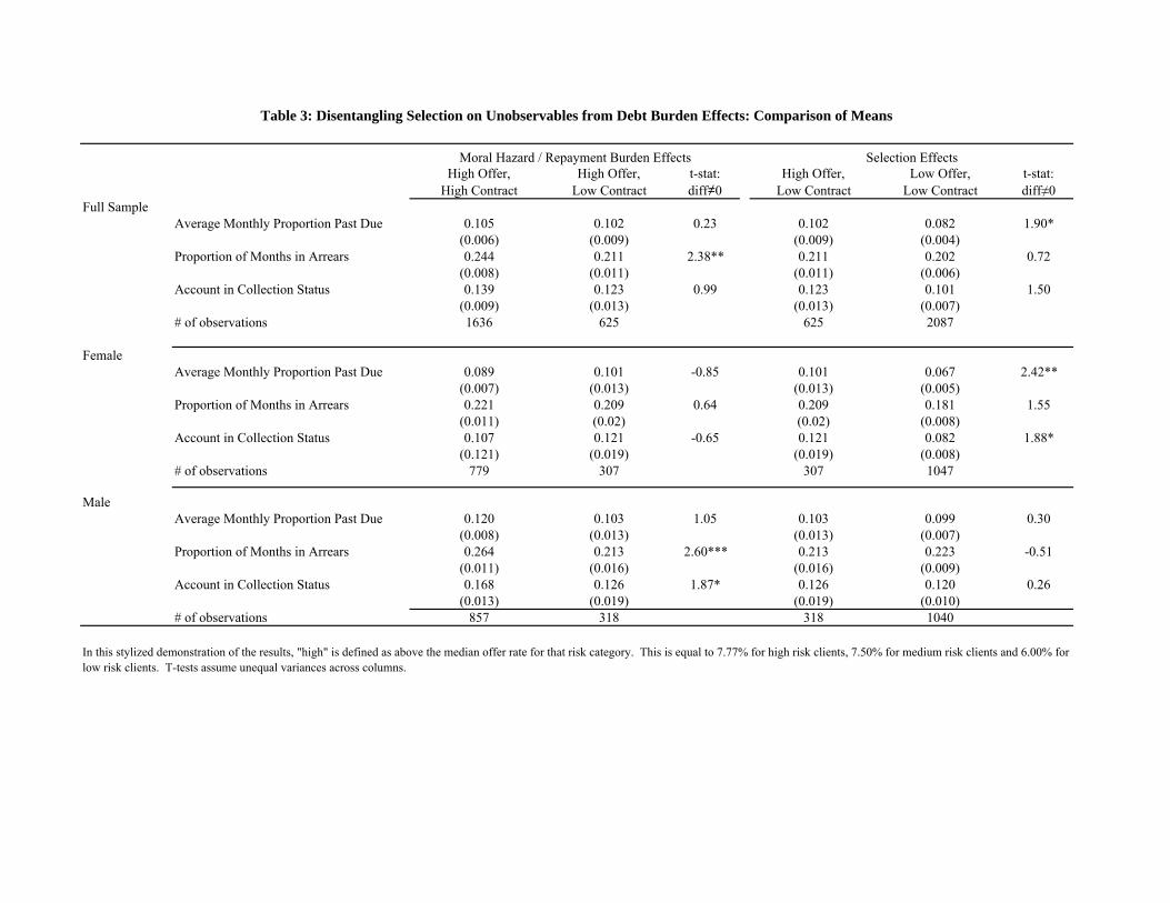
High Offer,High Contract
High Offer,Low Contract
t-stat:diff≠0
High Offer,Low Contract
Low Offer,Low Contract
t-stat:diff≠0
Full SampleAverage Monthly Proportion Past Due 0.105 0.102 0.23 0.102 0.082 1.90*
(0.006) (0.009) (0.009) (0.004)Proportion of Months in Arrears 0.244 0.211 2.38** 0.211 0.202 0.72
(0.008) (0.011) (0.011) (0.006)Account in Collection Status 0.139 0.123 0.99 0.123 0.101 1.50
(0.009) (0.013) (0.013) (0.007)# of observations 1636 625 625 2087
FemaleAverage Monthly Proportion Past Due 0.089 0.101 -0.85 0.101 0.067 2.42**
(0.007) (0.013) (0.013) (0.005)Proportion of Months in Arrears 0.221 0.209 0.64 0.209 0.181 1.55
(0.011) (0.02) (0.02) (0.008)Account in Collection Status 0.107 0.121 -0.65 0.121 0.082 1.88*
(0.121) (0.019) (0.019) (0.008)# of observations 779 307 307 1047
MaleAverage Monthly Proportion Past Due 0.120 0.103 1.05 0.103 0.099 0.30
(0.008) (0.013) (0.013) (0.007)Proportion of Months in Arrears 0.264 0.213 2.60*** 0.213 0.223 -0.51
(0.011) (0.016) (0.016) (0.009)Account in Collection Status 0.168 0.126 1.87* 0.126 0.120 0.26
(0.013) (0.019) (0.019) (0.010)# of observations 857 318 318 1040
In this stylized demonstration of the results, "high" is defined as above the median offer rate for that risk category. This is equal to 7.77% for high risk clients, 7.50% for medium risk clients and 6.00% for low risk clients. T-tests assume unequal variances across columns.
Moral Hazard / Repayment Burden Effects Selection Effects
Table 3: Disentangling Selection on Unobservables from Debt Burden Effects: Comparison of Means
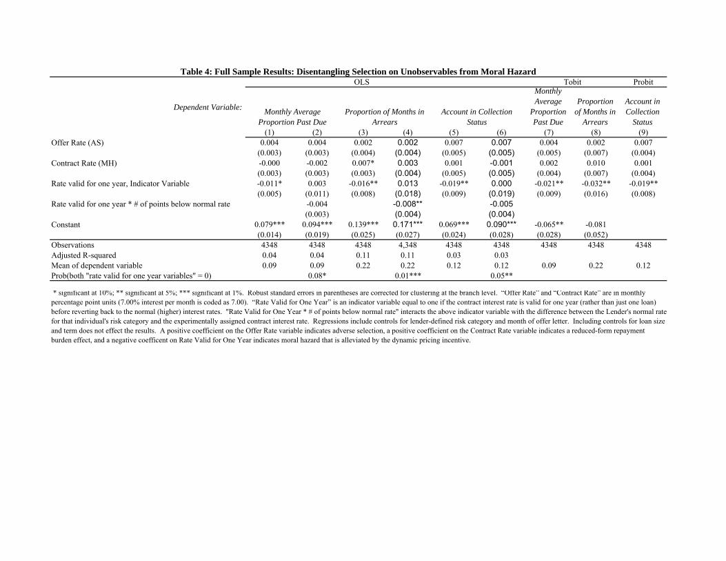
Probit
Dependent Variable:
Monthly Average
Proportion Past Due
Proportion of Months in
Arrears
Account in Collection
Status(1) (2) (3) (4) (5) (6) (7) (8) (9)
0.004 0.004 0.002 0.002 0.007 0.007 0.004 0.002 0.007(0.003) (0.003) (0.004) (0.004) (0.005) (0.005) (0.005) (0.007) (0.004)-0.000 -0.002 0.007* 0.003 0.001 -0.001 0.002 0.010 0.001(0.003) (0.003) (0.003) (0.004) (0.005) (0.005) (0.004) (0.007) (0.004)
Rate valid for one year, Indicator Variable -0.011* 0.003 -0.016** 0.013 -0.019** 0.000 -0.021** -0.032** -0.019**(0.005) (0.011) (0.008) (0.018) (0.009) (0.019) (0.009) (0.016) (0.008)
Rate valid for one year * # of points below normal rate -0.004 -0.008** -0.005(0.003) (0.004) (0.004)
0.079*** 0.094*** 0.139*** 0.171*** 0.069*** 0.090*** -0.065** -0.081(0.014) (0.019) (0.025) (0.027) (0.024) (0.028) (0.028) (0.052)
Observations 4348 4348 4348 4,348 4348 4348 4348 4348 4348Adjusted R-squared 0.04 0.04 0.11 0.11 0.03 0.03Mean of dependent variable 0.09 0.09 0.22 0.22 0.12 0.12 0.09 0.22 0.12Prob(both "rate valid for one year variables" = 0) 0.08* 0.01*** 0.05**
* significant at 10%; ** significant at 5%; *** significant at 1%. Robust standard errors in parentheses are corrected for clustering at the branch level. “Offer Rate” and “Contract Rate” are in monthly percentage point units (7.00% interest per month is coded as 7.00). “Rate Valid for One Year” is an indicator variable equal to one if the contract interest rate is valid for one year (rather than just one loan) before reverting back to the normal (higher) interest rates. "Rate Valid for One Year * # of points below normal rate" interacts the above indicator variable with the difference between the Lender's normal rate for that individual's risk category and the experimentally assigned contract interest rate. Regressions include controls for lender-defined risk category and month of offer letter. Including controls for loan size and term does not effect the results. A positive coefficient on the Offer Rate variable indicates adverse selection, a positive coefficient on the Contract Rate variable indicates a reduced-form repayment burden effect, and a negative coefficent on Rate Valid for One Year indicates moral hazard that is alleviated by the dynamic pricing incentive.
Offer Rate (AS)
Contract Rate (MH)
OLSTable 4: Full Sample Results: Disentangling Selection on Unobservables from Moral Hazard
Tobit
Constant
Monthly Average Proportion Past Due
Proportion of Months in Arrears
Account in Collection Status

Probit Probit
Dependent Variable:
Monthly Average
Proportion Past Due
Proportion of Months in
Arrears
Account in Collection
Status
Monthly Average
Proportion Past Due
Proportion of Months in
Arrears
Account in Collection
Status
Monthly Average
Proportion Past Due
Proportion of Months in
Arrears
Account in Collection
Status
Monthly Average
Proportion Past Due
Proportion of Months in Arrears
Account in Collection
Status(1) (2) (3) (4) (5) (6) (7) (8) (9) (10) (11) (12)
-0.002 -0.004 0.001 -0.005 -0.008 0.001 0.010*** 0.008* 0.013** 0.013** 0.013 0.011***(0.004) (0.005) (0.007) (0.006) (0.010) (0.007) (0.003) (0.005) (0.005) (0.006) (0.009) (0.004)0.005 0.014*** 0.010 0.010 0.021** 0.009 -0.005 -0.001 -0.009 -0.006 -0.003 -0.007*
(0.003) (0.005) (0.007) (0.006) (0.010) (0.006) (0.004) (0.005) (0.006) (0.006) (0.009) (0.004)-0.014 -0.025** -0.020 -0.033** -0.050** -0.020 -0.007 -0.006 -0.017 -0.008 -0.009 -0.016(0.009) (0.012) (0.015) (0.016) (0.023) (0.014) (0.008) (0.012) (0.012) (0.014) (0.025) (0.011)
0.108*** 0.178*** 0.092** -0.008 0.002 0.050*** 0.097*** 0.043 -0.121*** -0.176***(0.025) (0.040) (0.043) (0.043) (0.072) (0.015) (0.026) (0.027) (0.029) (0.057)
Observations 2215 2215 2215 2215 2215 2215 2133 2133 2133 2133 2133 2133R-squared 0.05 0.12 0.04 0.05 0.10 0.04
* significant at 10%; ** significant at 5%; *** significant at 1%. Robust standard errors in parentheses are corrected for clustering at the branch level. Regressions reported here are estimated using the base specification (equation 2) on samples split by gender. They include controls for lender-defined risk category and month of offer letter. Including controls for loan size and term does not effect the results.
Offer Rate (AS)
Contract Rate (MH)
Rate Valid for One Year (vs one loan)Constant
Table 5: Disentangling Selection on Unobservables from Moral HazardBy Gender
Male FemaleOLS Tobit OLS Tobit
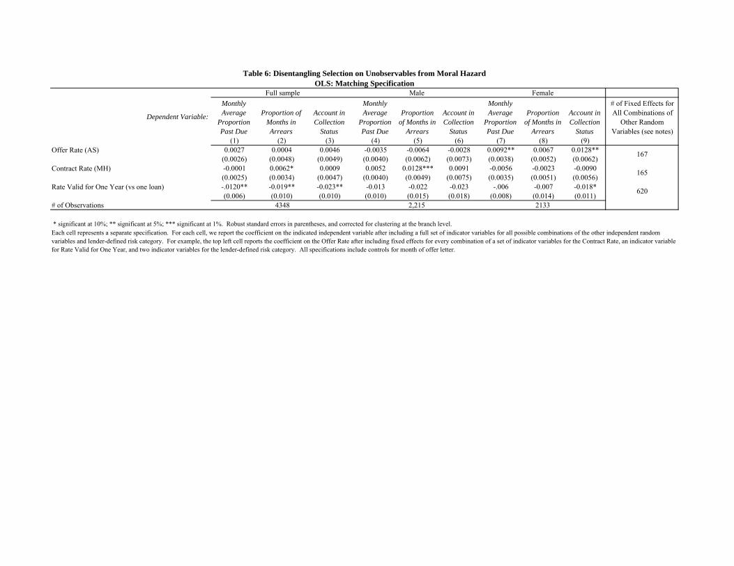
Dependent Variable:
Monthly Average
Proportion Past Due
Proportion of Months in Arrears
Account in Collection
Status
Monthly Average
Proportion Past Due
Proportion of Months in
Arrears
Account in Collection
Status
Monthly Average
Proportion Past Due
Proportion of Months in
Arrears
Account in Collection
Status
# of Fixed Effects for All Combinations of
Other Random Variables (see notes)
(1) (2) (3) (4) (5) (6) (7) (8) (9)0.0027 0.0004 0.0046 -0.0035 -0.0064 -0.0028 0.0092** 0.0067 0.0128**
(0.0026) (0.0048) (0.0049) (0.0040) (0.0062) (0.0073) (0.0038) (0.0052) (0.0062)-0.0001 0.0062* 0.0009 0.0052 0.0128*** 0.0091 -0.0056 -0.0023 -0.0090(0.0025) (0.0034) (0.0047) (0.0040) (0.0049) (0.0075) (0.0035) (0.0051) (0.0056)-.0120** -0.019** -0.023** -0.013 -0.022 -0.023 -.006 -0.007 -0.018*(0.006) (0.010) (0.010) (0.010) (0.015) (0.018) (0.008) (0.014) (0.011)
# of Observations
* significant at 10%; ** significant at 5%; *** significant at 1%. Robust standard errors in parentheses, and corrected for clustering at the branch level.
167
165
620
Table 6: Disentangling Selection on Unobservables from Moral HazardOLS: Matching Specification
Offer Rate (AS)
Contract Rate (MH)
Rate Valid for One Year (vs one loan)
FemaleMaleFull sample
21332,2154348
Each cell represents a separate specification. For each cell, we report the coefficient on the indicated independent variable after including a full set of indicator variables for all possible combinations of the other independent random variables and lender-defined risk category. For example, the top left cell reports the coefficient on the Offer Rate after including fixed effects for every combination of a set of indicator variables for the Contract Rate, an indicator variable for Rate Valid for One Year, and two indicator variables for the lender-defined risk category. All specifications include controls for month of offer letter.

Sample: Full Full Full Male Male Male Female Female Female
Dependent Variable:
Average Monthly
Proportion Past Due
Proportion of Months in Arrears
Account in Collection
Status
Average Monthly
Proportion Past Due
Proportion of Months in Arrears
Account in Collection
Status
Average Monthly
Proportion Past Due
Proportion of Months in Arrears
Account in Collection
Status(1) (2) (3) (4) (6) (7) (8) (10) (11)
Panel A: IVTotal Interest Cost, 000's Rands, at Offer Interest Rate 0.35* 0.29 0.66* -0.03 -0.00 0.41 0.74*** 0.65* 1.00**
(0.20) (0.28) (0.35) (0.29) (0.42) (0.51) (0.27) (0.35) (0.41)Total Interest Cost, 000's Rands, at Contract Interest Rate -0.00 0.10* 0.01 0.07 0.19** 0.14 -0.09 -0.02 -0.14
(0.04) (0.06) (0.08) (0.05) (0.08) (0.11) (0.06) (0.09) (0.10)Constant 0.09*** 0.19*** 0.09*** 0.10*** 0.21*** 0.09** 0.08*** 0.21*** 0.12***
(0.01) (0.02) (0.02) (0.02) (0.03) (0.04) (0.03) (0.03) (0.03)Observations 4348 4348 4348 2215 2215 2215 2133 2133 2133
Panel B: OLSTotal Interest Cost, 000's Rands, at Offer Interest Rate -0.12** 0.01 -0.08 -0.15* 0.06 0.06 -0.08 -0.02 -0.19
(0.06) (0.10) (0.10) (0.08) (0.14) (0.14) (0.06) (0.12) (0.13)Total Interest Cost, 000's Rands, at Contract Interest Rate -0.00 0.01 0.01 0.00 0.01 0.01 -0.01 0.01 0.02
(0.01) (0.01) (0.01) (0.01) (0.02) (0.01) (0.01) (0.02) (0.02)Constant 0.13*** 0.25*** 0.15*** 0.13*** 0.27*** 0.17*** 0.12*** 0.26*** 0.15***
(0.01) (0.01) (0.01) (0.01) (0.03) (0.02) (0.02) (0.02) (0.02)Observations 4348 4348 4348 2215 2215 2215 2133 2133 2133
0.05 0.10 0.03 0.05 0.11 0.03 0.05 0.10 0.03
Table 7: Disentangling Selection on Unobservables from Moral HazardIV
* significant at 10%; ** significant at 5%; *** significant at 1%. Robust standard errors in parentheses are corrected for clustering at the branch level. The two endogenous variables (total interest cost evaluated separately at the offer and contract rate) are instrumented with the offer rate and contract rate (please see equations 6-8 in the text). Regressions include controls for lender-defined risk category and month of offer letter. Including controls for loan size and term does not effect the results.

Demographic Control Variable:
(1) (2) (3) (4) (5) (6) (7) (8) (9) (10) (11) (12)Experimental Variables
Offer Rate (AS) 0.023 -0.252 0.089 0.176 0.079 -0.213 0.282 -0.341 2.700 -0.716 0.122 0.082(0.435) (0.537) (0.432) (0.530) (0.402) (0.410) (1.162) (1.325) (2.338) (4.218) (0.456) (0.495)
Contract Rate (MH) 0.415 0.716 0.482 0.660 0.260 0.557 0.269 0.652 -0.968 1.852 0.404 0.442(0.393) (0.508) (0.446) (0.527) (0.414) (0.440) (1.098) (1.283) (2.707) (4.600) (0.465) (0.523)
Rate Valid for One Year (vs one loan) -1.158 -0.706 -1.098 -1.920 -0.878 -1.081 -1.280 0.934 7.378 3.457 -1.165 -0.691(1.160) (1.510) (1.237) (1.434) (1.028) (1.252) (2.678) (4.049) (8.692) (12.814) (1.145) (1.465)
Female -2.985 -3.095 -2.558 -1.021 -2.215 -2.652 -1.887 -5.296 -2.821 -30.918 -2.667 -2.298(1.939) (2.585) (1.980) (3.110) (1.886) (2.631) (1.914) (7.409) (1.926) (28.386) (1.875) (3.073)
Demographic Variable (see column heading) -1.838 -2.040 -0.036 0.427 -1.761 -2.487 -0.172 -0.223 -0.001 -2.020 -0.015 -0.013(1.952) (2.854) (0.536) (0.741) (2.432) (3.909) (0.105) (0.157) (1.669) (3.019) (0.012) (0.018)
Female * Experimental VariablesFemale * Offer Rate (AS) 0.887* 1.369** 0.834* 0.637 0.902* 1.534** 0.763* 1.951 0.890** 6.945 0.807* 0.891
(0.456) (0.632) (0.460) (0.661) (0.480) (0.604) (0.455) (1.916) (0.445) (6.117) (0.447) (0.749)Female * Contract Rate (MH) -1.042** -1.575** -1.029** -1.440** -1.138** -1.783*** -0.977** -1.782 -1.040** -6.318 -0.967** -1.047
(0.476) (0.718) (0.497) (0.678) (0.482) (0.640) (0.486) (1.979) (0.474) (7.129) (0.479) (0.748)Female * Rate Valid for One Year (vs one loan) 0.813 -0.037 0.896 2.732 1.077 1.554 0.701 -3.491 0.603 8.148 0.730 -0.290
(1.350) (2.143) (1.343) (2.052) (1.351) (1.903) (1.336) (5.867) (1.353) (14.026) (1.328) (2.363)Demographic Control Variable * Experimental Variables
Demographic Variable * Offer Rate (AS) -0.135 0.415 -0.046 -0.084 -0.400 0.626 -0.008 0.008 -0.343 0.079 -0.002 -0.001(0.540) (0.796) (0.122) (0.164) (0.625) (0.853) (0.026) (0.030) (0.289) (0.522) (0.003) (0.003)
Demographic Variable * Contract Rate (AS) 0.195 -0.397 -0.009 -0.124 0.748 -0.279 0.006 -0.003 0.183 -0.166 0.001 0.001(0.511) (0.788) (0.141) (0.177) (0.583) (0.776) (0.026) (0.031) (0.325) (0.561) (0.003) (0.003)
Demographic Variable * Rate Valid for One Year -0.577 -1.442 -0.224 0.162 -1.577 -1.017 -0.002 -0.056 -1.077 -0.592 -0.002 -0.007(1.211) (1.897) (0.353) (0.431) (1.307) (2.104) (0.061) (0.092) (1.042) (1.530) (0.006) (0.009)
Female * Demographic Control VariableFemale * Demographic Variable 0.305 -1.217 1.155 0.083 3.457 -0.004
(3.234) (1.138) (4.167) (0.167) (3.460) (0.023)Female * Demographic Control Variable * Experimental Variables
Female * Demographic Variable * Offer Rate (AS) -1.079 0.111 -1.755 -0.029 -0.748 -0.001(0.951) (0.274) (1.080) (0.044) (0.758) (0.006)
Female * Demographic Variable * Contract Rate (AS) 1.181 0.277 1.777 0.020 0.654 0.001(1.033) (0.292) (1.196) (0.045) (0.882) (0.005)
Female * Demographic Variable * Rate Valid for One Year 1.797 -0.968 -1.049 0.102 -0.937 0.011(2.652) (0.654) (2.713) (0.125) (1.672) (0.015)
Constant 10.161*** 10.236*** 8.917*** 8.252*** 9.608*** 9.821*** 14.984*** 17.066** 9.240 25.704 10.281*** 10.122***(2.476) (2.791) (2.542) (2.986) (2.240) (2.546) (5.136) (7.222) (13.856) (25.009) (2.642) (3.133)
Observations 4317 4317 4317 4317 4348 4348 4348 4348 4348 4348 4348 4348R-squared 0.05 0.05 0.05 0.05 0.05 0.05 0.06 0.06 0.05 0.05 0.06 0.06
OLS, Dependent Variable: Monthly Average Percentage Past DueTable 8: Disentangling Selection on Unobservables from Moral Hazard, by Gender & Demographics
* significant at 10%; ** significant at 5%; *** significant at 1%. Robust standard errors in parentheses are corrected for clustering at the branch level. "Educated" is a binary indicator for the top 25% in years of education, predicted by the client's occupation. Regressions include controls for lender-defined risk category and month of offer letter. Including controls for loan size and term does not effect the results. The dependent variable here is defined in percentage point terms, not proportions, and hence equals 100x the variable used in other tables.
AgeEducatedDependants in HouseholdMarriedLog(Monthly Gross
Income) Tenure at Employment

Sample: All All Female Male(1) (2) (3) (4)
-0.0029*** -0.004*** -0.006*** -0.002(0.0004) (0.001) (0.002) (0.002)
Predicted Past Due Percentage -158.064** -268.010** -17.186(76.012) (122.971) (112.913)10.071 23.443* -4.948(8.852) (13.105) (13.786)
Observations 52985 52985 25221 27764
* significant at 10%; ** significant at 5%; *** significant at 1%. Robust standard errors in parentheses are corrected for clustering at the branch level. Predicted past due percentage is the predicted value for default from Table 10 OLS specifications. 4548 observations omitted because they were either missing income data for the non-applicants, received an upward-sloped yield curve on their offer letter, or had their letter returned by the postal system due to a bad address. Regressions include controls for lender-defined risk category and month of offer letter.
Offer Rate (AS)
Table 9: Selection on Observable InformationProbit, Dependent Variable: "Applied for Loan"
Offer Rate* Predicted Past Due Percentage
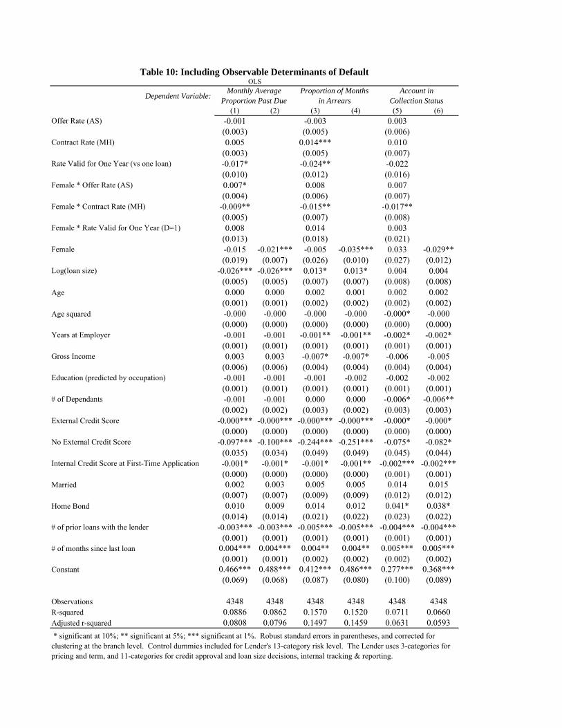
Dependent Variable:
(1) (2) (3) (4) (5) (6)-0.001 -0.003 0.003(0.003) (0.005) (0.006)0.005 0.014*** 0.010
(0.003) (0.005) (0.007)-0.017* -0.024** -0.022(0.010) (0.012) (0.016)0.007* 0.008 0.007(0.004) (0.006) (0.007)
-0.009** -0.015** -0.017**(0.005) (0.007) (0.008)0.008 0.014 0.003
(0.013) (0.018) (0.021)Female -0.015 -0.021*** -0.005 -0.035*** 0.033 -0.029**
(0.019) (0.007) (0.026) (0.010) (0.027) (0.012)-0.026*** -0.026*** 0.013* 0.013* 0.004 0.004
(0.005) (0.005) (0.007) (0.007) (0.008) (0.008)Age 0.000 0.000 0.002 0.001 0.002 0.002
(0.001) (0.001) (0.002) (0.002) (0.002) (0.002)Age squared -0.000 -0.000 -0.000 -0.000 -0.000* -0.000
(0.000) (0.000) (0.000) (0.000) (0.000) (0.000)Years at Employer -0.001 -0.001 -0.001** -0.001** -0.002* -0.002*
(0.001) (0.001) (0.001) (0.001) (0.001) (0.001)Gross Income 0.003 0.003 -0.007* -0.007* -0.006 -0.005
(0.006) (0.006) (0.004) (0.004) (0.004) (0.004)Education (predicted by occupation) -0.001 -0.001 -0.001 -0.002 -0.002 -0.002
(0.001) (0.001) (0.001) (0.001) (0.001) (0.001)# of Dependants -0.001 -0.001 0.000 0.000 -0.006* -0.006**
(0.002) (0.002) (0.003) (0.002) (0.003) (0.003)External Credit Score -0.000*** -0.000*** -0.000*** -0.000*** -0.000* -0.000*
(0.000) (0.000) (0.000) (0.000) (0.000) (0.000)No External Credit Score -0.097*** -0.100*** -0.244*** -0.251*** -0.075* -0.082*
(0.035) (0.034) (0.049) (0.049) (0.045) (0.044)Internal Credit Score at First-Time Application -0.001* -0.001* -0.001* -0.001** -0.002*** -0.002***
(0.000) (0.000) (0.000) (0.000) (0.001) (0.001)Married 0.002 0.003 0.005 0.005 0.014 0.015
(0.007) (0.007) (0.009) (0.009) (0.012) (0.012)Home Bond 0.010 0.009 0.014 0.012 0.041* 0.038*
(0.014) (0.014) (0.021) (0.022) (0.023) (0.022)# of prior loans with the lender -0.003*** -0.003*** -0.005*** -0.005*** -0.004*** -0.004***
(0.001) (0.001) (0.001) (0.001) (0.001) (0.001)# of months since last loan 0.004*** 0.004*** 0.004** 0.004** 0.005*** 0.005***
(0.001) (0.001) (0.002) (0.002) (0.002) (0.002)0.466*** 0.488*** 0.412*** 0.486*** 0.277*** 0.368***(0.069) (0.068) (0.087) (0.080) (0.100) (0.089)
Observations 4348 4348 4348 4348 4348 4348R-squared 0.0886 0.0862 0.1570 0.1520 0.0711 0.0660Adjusted r-squared 0.0808 0.0796 0.1497 0.1459 0.0631 0.0593
Constant
* significant at 10%; ** significant at 5%; *** significant at 1%. Robust standard errors in parentheses, and corrected for clustering at the branch level. Control dummies included for Lender's 13-category risk level. The Lender uses 3-categories for pricing and term, and 11-categories for credit approval and loan size decisions, internal tracking & reporting.
Table 10: Including Observable Determinants of DefaultOLS
Monthly Average Proportion Past Due
Proportion of Months in Arrears
Account in Collection Status
Offer Rate (AS)
Contract Rate (MH)
Rate Valid for One Year (vs one loan)
Log(loan size)
Female * Offer Rate (AS)
Female * Contract Rate (MH)
Female * Rate Valid for One Year (D=1)

Sample:(1) (2) (3) (4) (5) (6) (7) (8) (9)
Offer Rate (AS) 0.008** 0.004 0.004 0.014*** 0.010*** 0.010*** 0.001 -0.002 -0.002(0.003) (0.003) (0.003) (0.004) (0.003) (0.003) (0.005) (0.004) (0.004)
Contract Rate (MH) 0.000 0.004 0.000 -0.005 -0.001 -0.005 0.005 0.008* 0.005(0.003) (0.003) (0.003) (0.004) (0.004) (0.004) (0.003) (0.004) (0.003)-0.011* -0.011* -0.013 -0.007 -0.007 -0.006 -0.015 -0.015 -0.023(0.006) (0.006) (0.010) (0.008) (0.008) (0.011) (0.010) (0.010) (0.017)0.001 0.000 0.003 0.001 -0.001 -0.001
(0.002) (0.001) (0.002) (0.002) (0.003) (0.003)-0.001*** -0.001*** -0.001
(0.000) (0.000) (0.000)-0.001*** -0.001*** -0.001
(0.000) (0.000) (0.000)0.001 -0.000 0.002
(0.001) (0.001) (0.002)Constant 0.078*** 0.083*** 0.105*** 0.040** 0.046*** 0.070*** 0.119*** 0.121*** 0.142***
(0.018) (0.017) (0.014) (0.017) (0.016) (0.015) (0.034) (0.032) (0.025)Observations 4317 4317 4317 2119 2119 2119 2198 2198 2198R-squared 0.05 0.05 0.05 0.06 0.06 0.05 0.06 0.06 0.06
* significant at 10%; ** significant at 5%; *** significant at 1%. Robust standard errors in parentheses are corrected for clustering at the branch level. Regressions include controls for lender-defined risk category and month of offer letter. Including controls for loan size and term does not effect the results.
All MaleFemale
Table 11: Do Information Asymmetries Diminish for Clients with More Frequent Borrowing History?OLS, Dependent Variable: Monthly Average Proportion Past Due
Offer Rate*# of prior loans
Rate Valid for One Year*# of prior loans
Rate Valid for One Year (vs one loan)
# of prior loans with the lender
Contract Rate*# of prior loans
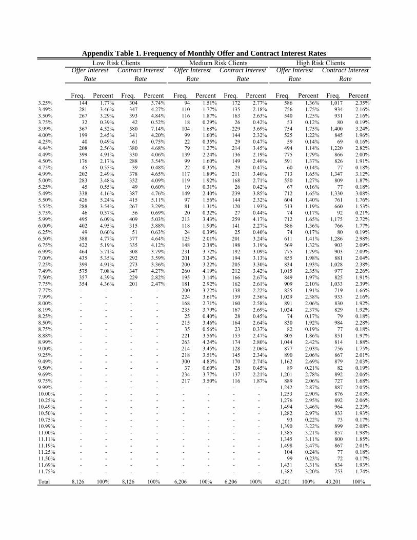
Freq. Percent Freq. Percent Freq. Percent Freq. Percent Freq. Percent Freq. Percent3.25% 144 1.77% 304 3.74% 94 1.51% 172 2.77% 586 1.36% 1,017 2.35%3.49% 281 3.46% 347 4.27% 110 1.77% 135 2.18% 756 1.75% 934 2.16%3.50% 267 3.29% 393 4.84% 116 1.87% 163 2.63% 540 1.25% 931 2.16%3.75% 32 0.39% 42 0.52% 18 0.29% 26 0.42% 53 0.12% 80 0.19%3.99% 367 4.52% 580 7.14% 104 1.68% 229 3.69% 754 1.75% 1,400 3.24%4.00% 199 2.45% 341 4.20% 99 1.60% 144 2.32% 525 1.22% 845 1.96%4.25% 40 0.49% 61 0.75% 22 0.35% 29 0.47% 59 0.14% 69 0.16%4.44% 208 2.56% 380 4.68% 79 1.27% 214 3.45% 494 1.14% 1,220 2.82%4.49% 399 4.91% 330 4.06% 139 2.24% 136 2.19% 775 1.79% 866 2.00%4.50% 176 2.17% 288 3.54% 99 1.60% 149 2.40% 591 1.37% 826 1.91%4.75% 45 0.55% 39 0.48% 22 0.35% 29 0.47% 60 0.14% 77 0.18%4.99% 202 2.49% 378 4.65% 117 1.89% 211 3.40% 713 1.65% 1,347 3.12%5.00% 283 3.48% 332 4.09% 119 1.92% 168 2.71% 550 1.27% 809 1.87%5.25% 45 0.55% 49 0.60% 19 0.31% 26 0.42% 67 0.16% 77 0.18%5.49% 338 4.16% 387 4.76% 149 2.40% 239 3.85% 712 1.65% 1,330 3.08%5.50% 426 5.24% 415 5.11% 97 1.56% 144 2.32% 604 1.40% 761 1.76%5.55% 288 3.54% 267 3.29% 81 1.31% 120 1.93% 513 1.19% 660 1.53%5.75% 46 0.57% 56 0.69% 20 0.32% 27 0.44% 74 0.17% 92 0.21%5.99% 495 6.09% 409 5.03% 213 3.43% 259 4.17% 712 1.65% 1,175 2.72%6.00% 402 4.95% 315 3.88% 118 1.90% 141 2.27% 586 1.36% 766 1.77%6.25% 49 0.60% 51 0.63% 24 0.39% 25 0.40% 74 0.17% 80 0.19%6.50% 388 4.77% 377 4.64% 125 2.01% 201 3.24% 611 1.41% 1,286 2.98%6.75% 422 5.19% 335 4.12% 148 2.38% 198 3.19% 569 1.32% 903 2.09%6.99% 464 5.71% 308 3.79% 231 3.72% 192 3.09% 775 1.79% 903 2.09%7.00% 435 5.35% 292 3.59% 201 3.24% 194 3.13% 855 1.98% 881 2.04%7.25% 399 4.91% 273 3.36% 200 3.22% 205 3.30% 834 1.93% 1,028 2.38%7.49% 575 7.08% 347 4.27% 260 4.19% 212 3.42% 1,015 2.35% 977 2.26%7.50% 357 4.39% 229 2.82% 195 3.14% 166 2.67% 849 1.97% 825 1.91%7.75% 354 4.36% 201 2.47% 181 2.92% 162 2.61% 909 2.10% 1,033 2.39%7.77% - - - - 200 3.22% 138 2.22% 825 1.91% 719 1.66%7.99% - - - - 224 3.61% 159 2.56% 1,029 2.38% 933 2.16%8.00% - - - - 168 2.71% 160 2.58% 891 2.06% 830 1.92%8.19% - - - - 235 3.79% 167 2.69% 1,024 2.37% 829 1.92%8.25% - - - - 25 0.40% 28 0.45% 74 0.17% 79 0.18%8.50% - - - - 215 3.46% 164 2.64% 830 1.92% 984 2.28%8.75% - - - - 35 0.56% 23 0.37% 82 0.19% 77 0.18%8.88% - - - - 221 3.56% 153 2.47% 805 1.86% 851 1.97%8.99% - - - - 263 4.24% 174 2.80% 1,044 2.42% 814 1.88%9.00% - - - - 214 3.45% 128 2.06% 877 2.03% 756 1.75%9.25% - - - - 218 3.51% 145 2.34% 890 2.06% 867 2.01%9.49% - - - - 300 4.83% 170 2.74% 1,162 2.69% 879 2.03%9.50% - - - - 37 0.60% 28 0.45% 89 0.21% 82 0.19%9.69% - - - - 234 3.77% 137 2.21% 1,201 2.78% 892 2.06%9.75% - - - - 217 3.50% 116 1.87% 889 2.06% 727 1.68%9.99% - - - - - - - - 1,242 2.87% 887 2.05%10.00% - - - - - - - - 1,253 2.90% 876 2.03%10.25% - - - - - - - - 1,276 2.95% 892 2.06%10.49% - - - - - - - - 1,494 3.46% 964 2.23%10.50% - - - - - - - - 1,282 2.97% 833 1.93%10.75% - - - - - - - - 93 0.22% 73 0.17%10.99% - - - - - - - - 1,390 3.22% 899 2.08%11.00% - - - - - - - - 1,385 3.21% 857 1.98%11.11% - - - - - - - - 1,345 3.11% 800 1.85%11.19% - - - - - - - - 1,498 3.47% 867 2.01%11.25% - - - - - - - - 104 0.24% 77 0.18%11.50% - - - - - - - - 99 0.23% 72 0.17%11.69% - - - - - - - - 1,431 3.31% 834 1.93%11.75% - - - - - - - - 1,382 3.20% 753 1.74%
Total 8,126 100% 8,126 100% 6,206 100% 6,206 100% 43,201 100% 43,201 100%
Appendix Table 1. Frequency of Monthly Offer and Contract Interest RatesLow Risk Clients Medium Risk Clients High Risk Clients
Offer Interest Rate
Contract Interest Rate
Offer Interest Rate
Contract Interest Rate
Offer Interest Rate
Contract Interest Rate

Probit
Dependent Variable:Monthly Average
Proportion Past Due
Proportion of Months in Arrears
Account in Collection
Status
Monthly Average
Proportion Past Due
Proportion of Months in
Arrears
Account in Collection
Status(1) (2) (3) (4) (5) (6)
0.007 0.005 0.012 0.007 0.004 0.011(0.005) (0.006) (0.008) (0.009) (0.014) (0.007)-0.006 0.001 -0.003 -0.006 0.002 -0.003(0.005) (0.006) (0.008) (0.009) (0.014) (0.007)-0.010* -0.021** -0.017** -0.023** -0.040** -0.016**(0.005) (0.009) (0.007) (0.011) (0.020) (0.007)
0.087*** 0.149*** 0.067*** -0.035 -0.058(0.016) (0.029) (0.023) (0.033) (0.064)
Observations 2715 2715 2715 2715 2715 2,715R-squared 0.06 0.12 0.04
* significant at 10%; ** significant at 5%; *** significant at 1%. Robust standard errors in parentheses, and corrected for clustering at the branch level. Includes controls for lender-defined risk category and month of offer letter. Including controls for loan size and term do not effect results.
Contract Rate (MH)
Rate Valid for One Year (vs one loan)Constant
Offer Rate (AS)
OLS Tobit
Appendix Table 2: Table 4 Results, Sample RestrictedSample Restricted to Those Offered ≤ 7.75%, the Ceiling for Low Risk Clients

Sample: All All Female Male
Full SampleOffer Rate = Contract
RateOffer Rate = Contract
RateOffer Rate = Contract
Rate(1) (2) (3) (4)
Offer Interest Rate 0.004** 0.004** 0.004* 0.004(0.002) (0.002) (0.002) (0.003)
Rate valid for one year (Indicator Variable) -0.011* -0.005 -0.010 -0.001(0.005) (0.007) (0.009) (0.010)
Constant 0.079*** 0.074*** 0.042** 0.104***(0.014) (0.018) (0.018) (0.030)
Observations 4348 2619 1280 1339R-squared 0.04 0.05 0.05 0.05
Appendix Table 3. Primary Analysis with Offer Rate Alone (No Contract Rate)Dependent Variable: Monthly Average Proportion Past Due
* significant at 10%; ** significant at 5%; *** significant at 1%. Robust standard errors in parentheses, and corrected for clustering at the branch level. This table repeats the primary specification, but ignores the contract rate. Hence, the offer rates results presented here do not disentangle selection effects from repayment burden effects as before, but rather present a reduced-form combination of the two effects. Includes controls for lender-defined risk category and month of offer letter. Including controls for loan size and term do not effect results.