Observations of Convection Initiation “Failure” from the 12 June ...

Observations of Convection Initiation “Failure” from the 12 June 2002IHOP Deployment

PAUL MARKOWSKI AND CHRISTINA HANNON

Department of Meteorology, The Pennsylvania State University, University Park, Pennsylvania

ERIK RASMUSSEN

Cooperative Institute for Mesoscale Meteorological Studies, Norman, Oklahoma

(Manuscript received 16 August 2004, in final form 19 October 2004)

ABSTRACT

Observations of the development of cumulus convection, which reached depths of several kilometers butfailed to develop into sustained, precipitating, cumulonimbus clouds—an event the authors term “convec-tion initiation failure”—are presented from the 12 June 2002 International H2O Project (IHOP) case. Theinvestigation relies heavily on remote and in situ data obtained by mobile, truck-borne Doppler radars,mobile mesonets, mobile soundings, and stereo cloud photogrammetry.

Data collection was focused in northwestern Oklahoma near the intersection of an outflow boundary anddryline. Thunderstorms developed along the dryline during the late afternoon approximately 40 km east ofthe domain intensively observed by the ground-based observing systems. Farther west, within the region ofdense observations analyzed herein, cumulus congestus clouds formed along an outflow boundary. Mul-tiple-Doppler wind syntheses revealed that the boundary layer vertical velocity field was dominated bythermals rather than by circulations associated with the mesoscale boundaries. In spite of this observation,deep cumulus cloud development was confined to the mesoscale boundaries. Trajectories into the deepcumulus clouds that developed along the outflow boundary were much more vertical than those entering theshallow cumulus clouds observed away from the outflow boundary. It is hypothesized that the role of theoutflow boundary in promoting deep cumulus cloud formation was to promote updrafts that were lesssusceptible to the dilution of equivalent potential temperature, which controls the potential buoyancy,vertical velocity, and depth that can be realized by the clouds. It is also hypothesized that the lack of apersistent, spatially continuous corridor of mesoscale ascent along the outflow boundary and associatedmoisture upwelling contributed to convection initiation failure along the outflow boundary.

1. Introduction

The initiation of deep moist convection, commonlyreferred to as convection initiation, requires that par-cels of air reach their level of free convection (LFC)and then achieve and maintain positive buoyancy overa significant upward vertical excursion. The locationand timing of convection initiation is of acute interest toforecasters owing to the obvious association betweenconvective storms and precipitation and severeweather, in addition to less obvious impacts, such as theeffects of convection on energy demand, future numeri-

cal weather predictions, and occasionally subsequentconvective storm development.

The presence of an LFC and convective availablepotential energy (CAPE) requires a relatively largelower- to middle-tropospheric lapse rate (larger thanthe moist adiabatic lapse rate, on average) and low-level moisture. The difficulty in making detailed pre-dictions of convection initiation ultimately arises fromthe fact that the presence of CAPE is not a sufficientcondition for convection initiation. Air typically re-quires some forced ascent in order to reach its LFC,owing to the presence of at least some convective inhi-bition (CIN) on most environmental soundings. Deepmoist convection commonly is initiated along conver-gent mesoscale boundaries (Wilson and Schreiber1986), such as fronts (e.g., Hobbs and Persson 1982;Koch 1984; Parsons et al. 1987; Koch et al. 1997; Koch

Corresponding author address: Dr. Paul Markowski, The Penn-sylvania State University, 503 Walker Building, University Park,PA 16802.E-mail: [email protected]

JANUARY 2006 M A R K O W S K I E T A L . 375

© 2006 American Meteorological Society

MWR3059

and Clark 1999), drylines (e.g., Rhea 1966; Ogura andChen 1977; Schaefer 1986; Hane et al. 1997; Ziegler etal. 1997), outflow boundaries (e.g., Purdom 1976; Mat-thews 1981; Droegemeier and Wilhelmson 1985;Kingsmill 1995), or sea and land breezes (e.g., Lher-mitte and Gilet 1975; Purdom 1976; Wakimoto and At-kins 1994; Atkins et al. 1995; Fankhauser et al. 1995;Kingsmill 1995). Convective storms also have been ob-served to be initiated by circulations driven by differ-ential heating [e.g., cloudy–clear air boundaries (e.g.,Segal et al. 1986), heating of sloped terrain (e.g., Bra-ham and Draginis 1960; Orville 1964; Raymond andWilkening 1980), horizontal sensible heat flux varia-tions (e.g., Segal and Arritt 1992)] and forced lifting bygravity waves or bores (e.g., Ferretti et al. 1988; Car-bone et al. 1990; Karyampudi et al. 1995).

Synoptic-scale dynamics often prime the mesoscaleenvironment for convection initiation by way of large-scale, mean ascent, which tends to reduce CIN anddeepen the low-level moist layer. On the other hand,synoptic-scale dynamics also can discourage convectioninitiation by way of mean subsidence, which has theopposite effects. Large-scale vertical motions can beanticipated reasonably well from model guidance andfrom the diagnosis of quasigeostrophic forcings. Thus,in forecasting convection initiation—a distinctly meso-scale process—it often is important to identify synoptic-scale disturbances (Doswell 1987).

Unfortunately, producing skillful convection initia-tion forecasts is not as simple as the above discussionmay suggest. For example, although mesoscale bound-aries like those cited above are relatively easy to iden-tify using operational observing systems, rarely doesconvection develop along the entire length of suchboundaries. Instead, convective storms typically are ini-tiated along only limited segments of mesoscale bound-aries. Another example of the difficulty in convectioninitiation forecasting is with regard to the CIN mea-sured on “environmental” soundings (e.g., Weckwerthet al. 1996). In some cases, CIN is observed to be en-tirely absent, yet deep cumulus convection still fails todevelop (e.g., Ziegler and Rasmussen 1998). In othercases, nearby soundings indicate that significant CINremains, yet deep cumulus clouds or thunderstorms areobserved. Perhaps there are issues pertaining to sound-ing representativeness—mesoscale heterogeneities inthe temperature and moisture fields generally are notresolved in real time nor in ex post facto studies. Orperhaps it is the assumptions made in using soundingsto assess the likelihood of convection that are problem-atic. For example, mixing occurs along trajectories ofair rising to the saturation level and LFC. Thus, as

noted by Ziegler and Rasmussen (1998), convection ini-tiation is not as simple as reaching the so-called con-vective temperature or eliminating CIN, although re-ducing CIN is certainly one aspect of creating an envi-ronment favorable for convection initiation. Thekinematic fields in convective storm environments alsoare quite heterogeneous. Convective storms have beenobserved to develop where horizontal convective rollsintersect mesoscale boundaries (e.g., Atkins et al.1995), and vertical vortices also have been identified inclose proximity to growing cumulonimbi (e.g.,Kingsmill 1995).

Increases in convection initiation forecasting skill ar-guably have advanced at a slower rate than our abilityto anticipate convective storm type, organization, andassociated severe weather threats. The convection ini-tiation component of the International H2O Project(IHOP; Weckwerth et al. 2004) was designed to obtaindense observations of temperature, moisture, and windwithin the atmospheric boundary layer in order to im-prove our understanding of the processes responsiblefor the aforementioned difficulties in anticipating con-vection initiation. In this paper, we investigate a con-vection initiation “failure” case from IHOP on 12 June2002. Herein “failure” is defined as the failure of cu-mulus convection to develop into sustained cumulon-imbus clouds.

The analysis presented in this paper is based on ob-servations largely collected by ground-based instru-mentation. Four truck-borne Doppler radars were ar-ranged in a diamond-shaped configuration (�18 km ona side), with mobile soundings, a mobile wind profiler,a mobile radiometer, mobile mesonets, and two aircraftobtaining kinematic and thermodynamic measurementswithin this intensive observation region (IOR) definedby the four radars. The 12 June 2002 case is of interestbecause cumulus congestus clouds developed within theIOR, but these clouds failed to develop further intocumulonimbi. Approximately 40 km east of the IOR,severe, precipitating convection was initiated, but theprocesses responsible for convection initiation there arenot the subject of this paper. Airborne Doppler radarobservations of convection initiation east of the IORwill be presented in a future paper (T. Weckwerth 2004,personal communication).

The observations obtained in this case permit an in-vestigation of the details of convection initiation fail-ure—details that have contributed to the difficulties inmaking skillful, precise predictions of the location andtiming of the onset of deep moist convection. High-resolution wind syntheses derived from the multiple-Doppler radars allow for accurate trajectory calcula-tions and permit credible retrievals of thermodynamic

376 M O N T H L Y W E A T H E R R E V I E W VOLUME 134

information. Stereophotogrammetric cloud observa-tions combined with the retrieved wind fields permit aquantitative analysis of the relationships betweenboundary layer kinematic structures and cloud devel-opment. With the aid of these datasets, the followingquestions will be addressed:

• What are the relationships between boundary layerkinematic structures (e.g., rolls, vertical vortices, up-drafts) and thermodynamic fields, including the cloudfield?

• How do mesoscale boundaries interact with the con-vective boundary layer?

• What processes lead to the largest vertical excursionsof air parcel trajectories?

In section 2, the data and analysis techniques are de-scribed. In section 3, a synoptic and mesoscale overviewof the 12 June 2002 case is presented. In sections 4–6,the relationships among kinematic and thermodynamicboundary layer structures and cloud development areanalyzed. Section 7 contains a discussion of the resultsas they pertain to convection initiation. Last, section 8offers a summary, conclusions, and some suggestionsfor future work.

2. Data and analysis techniques

a. Remote and in situ observing systems

The observations utilized in this study were obtainedby a wide variety of observing platforms (Fig. 1). Four

mobile radars collected data continuously from 1936 to2130 UTC. Three of the mobile radars [two DopplerOn Wheels (DOW2 and DOW3) radars and an X-banddual-polarimetric radar (XPOL)] were similar to thosedescribed by Wurman et al. (1997). The wavelength,stationary half-power beamwidth, and Nyquist velocitywere 3 cm, 0.93°, and 16.0 m s�1, respectively. Volumeswere completed every 90 s, during which time 16 eleva-tion angles were scanned from 0.5° to 14.5°. The azi-muth interval between each ray was 0.7°. Within theanalysis region, the data spacing (note the oversam-pling implied by the sampling intervals in azimuth andelevation angle) was approximately 70–250 m in thehorizontal and 50–300 m in the vertical. The fourthmobile radar [Shared Mobile Atmospheric Researchand Teaching (SMART) Radar (SR1)] has been de-scribed by Biggerstaff and Guynes (2000). The wave-length, stationary half-power beamwidth, and Nyquistvelocity were 5 cm, 1.5°, and 14.6 m s�1, respectively.Volumes were completed every 180 s, during whichtime 15 elevation angles were scanned from 0.5° to25.2°. The azimuth interval between each ray was 1.0°.Within the analysis region, the data spacing was ap-proximately 70–350 m in the horizontal and 50–400 m inthe vertical.

Nine automobile-borne surface observing systems(“mobile mesonets”; Straka et al. 1996) obtained tem-perature, relative humidity, pressure, and wind velocitymeasurements with a frequency of 1 Hz. Additional insitu measurements were provided by three mobile

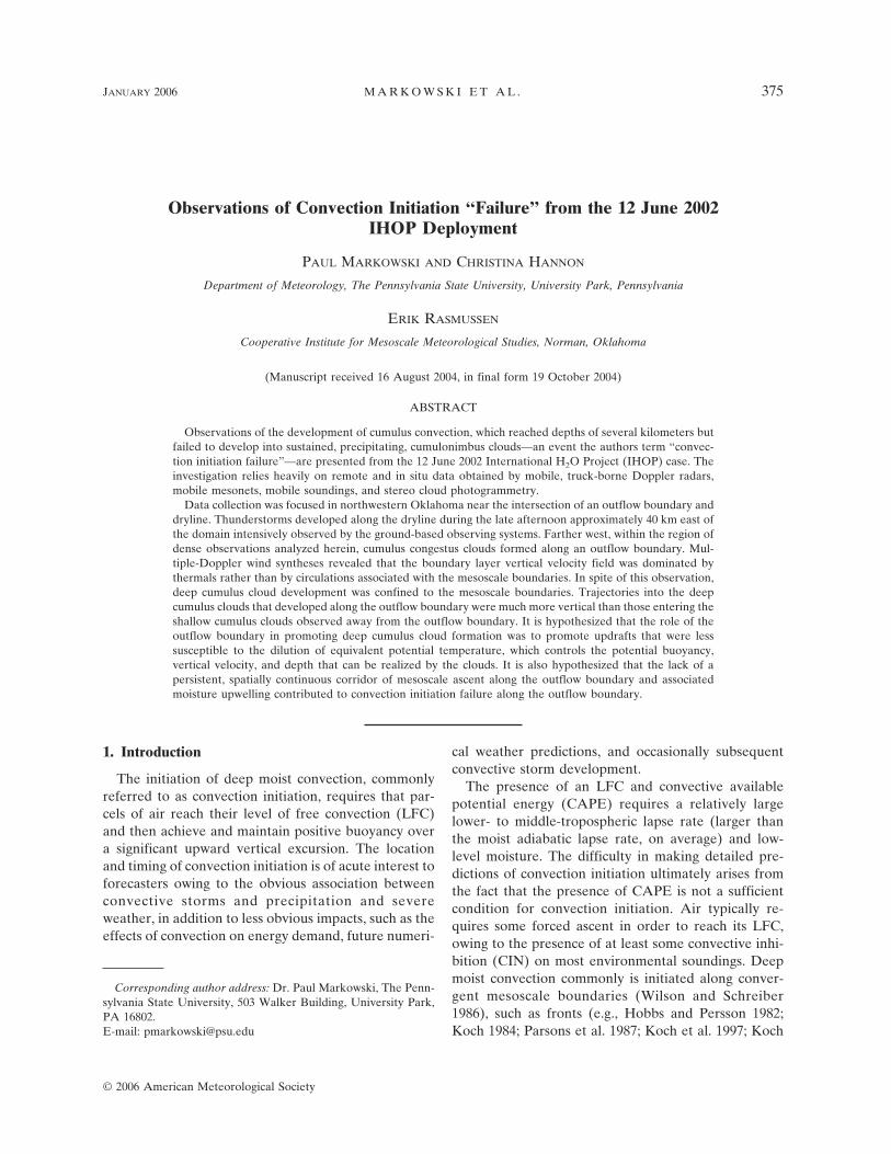
FIG. 1. Observations obtained during the 1930–2130 UTC mobile radar deployment on 12 Jun 2002. The locationsof camera, mobile mesonet, dropsonde, rawinsonde, aircraft (NRL P-3 and UWKA), mobile radar (DOW2,DOW3, XPOL, SR1), and mobile radiometer (DRI) observations are indicated using the symbology defined in thelegend. The square encloses the 50 � 50 km2 mobile radar analysis region (the same region indicated in Figs. 3, 4,and 6). The positions of mesoscale boundaries at 2100 UTC also are overlaid.


sounding units [one Mobile Cross-Chain Loran Atmo-spheric Sounding System (M-CLASS; Frederickson1993) and two Mobile GPS/Loran Atmospheric Sound-ing Systems (M-GLASS; Bluestein 1993)] and drop-sondes (Hock and Franklin 1999) released from theFlight International Learjet, which was flying at ap-proximately 700 mb. Two aircraft, the Naval ResearchLaboratory (NRL) P-3 and the University of WyomingKing Air (UWKA), also provided direct thermody-namic observations above the surface (1-Hz fre-quency). The flight tracks are displayed in Fig. 1.

Two video cameras (CAM1 and CAM2) obtainedcloud imagery for the duration of the deployment. Onecamera was positioned near the XPOL radar, lookingnorthward, and the other camera was positioned nearSR1, looking westward (Fig. 1). Clouds were mappedusing the stereo photogrammetric cloud mapping tech-niques described by Rasmussen et al. (2003). Integratedliquid water content data from the Desert ResearchInstitute (DRI) mobile radiometer (Huggins 1995),where available, were used to confirm the photogram-metrically determined cloud positions.

b. Radar data objective analysis and wind synthesis

Radial velocity data were edited to remove errorscaused by low signal-to-noise ratio, second-trip echoes,sidelobes, ground clutter, and velocity aliasing. The cor-rect azimuth orientations of the radars were obtainedby comparisons of the ground clutter patterns to theknown positions of landmarks visible in the clutter pat-terns. The orientations of two of the radars (DOW2 andXPOL) were confirmed by solar alignment scans (Ar-nott et al. 2003). The propagation of azimuth errors intothe wind synthesis is explored in appendix A.

Radial velocity data were interpolated to two differ-ent Cartesian grids. One was a coarse 50 � 50 � 2 km3

grid having a horizontal and vertical grid spacing of 200m (Fig. 1). This grid encompassed nearly all of the re-gion sampled by two radars, within which dual-Doppleranalysis was possible, and defines the “IOR” describedin section 1. A finer grid was nested within the largergrid, where the spatial resolution of the radars wasgreatest. It spanned 24 � 24 � 2 km3, had a horizontaland vertical grid spacing of 100 m, and encompassed theregion sampled by all four mobile radars (i.e., the re-gion containing the most accurate wind syntheses). Thelowest level of both grids was 100 m above the meanelevation of the radars.

The interpolation was accomplished by way of a Bar-nes objective analysis (Barnes 1964; Koch et al. 1983),using an isotropic, spherical weight function andsmoothing parameter, �, of 0.36 km2. This choice ofsmoothing parameter yields a 40% theoretical response

for features having a wavelength of 2.0 km, which isapproximately 4 times the data spacing at a range of 30km from the radars (approximately the coarsest dataspacing in the dual-Doppler analysis region). This rela-tively conservative choice for � follows the recommen-dations of Trapp and Doswell (2000). For computa-tional reasons, data beyond a “cutoff” radius, Rc, of1.25 km from each grid point were not considered in thecalculation of the weights, even though the theoreticalcontribution to the weight function remains nonzeroand positive, albeit very small, for distances between adatum and grid point greater than Rc. Objective analy-ses were produced using other smoothing parametersand cutoff radii. The sensitivity of the objective analysisto the choice of � and Rc is investigated in appendix A.

Advection was removed from the objectively ana-lyzed radial velocity grids, whereby an “optimal” ad-vection velocity was determined by minimizing the lo-cal time tendencies of the velocity components (Mate-jka 2002). The sensitivity of the wind syntheses to thespecification of the advection velocity also is exploredin appendix A.

Three-dimensional wind syntheses were producedusing the overdetermined dual-Doppler approach andthe anelastic mass continuity equation (integrated up-ward), rather than a direct triple- or quadruple-Doppler solution. The former approach has several ad-vantages over the latter approaches, as demonstratedby Kessinger et al. (1987). The wind syntheses aboveapproximately 1.7 km were not considered to be veryreliable due to the fact that the signal-to-noise ratiofrom two of the radars (DOW3 and XPOL) was unac-ceptably small at these elevations. The time resolutionof the analyses is 90 s, over which time synchronizedscans were completed by three of the four radars(DOW2, DOW3, and XPOL). Every other analysis(180-s intervals) is obtained using a four-radar overde-termined dual-Doppler solution. Comparisons betweenthe synthesized wind fields and in situ wind measure-ments made by the UWKA and NRL P-3 (smoothed sothat the scales represented in the velocity time serieswere comparable to those resolved in the radar-derivedwind syntheses) indicated good agreement between theradar-derived wind fields and those measured by theother two platforms.

c. Pressure and buoyancy retrieval

Within the 24 � 24 � 2 km3 domain, where windsyntheses were the most trustworthy, dynamic retriev-als of pressure and buoyancy perturbations were per-formed. The technique used was identical to that de-scribed by Gal-Chen (1978) and later used by Hane andRay (1985), among others. Indirect and direct methods


were undertaken to check the validity of the retrievedpressure and buoyancy fields. The results of momen-tum checking (Gal-Chen 1978), autocorrelation analy-sis, and comparisons to in situ observations are dis-cussed in appendix B.

It is crucial that the time derivatives of the velocitycomponents be accurately known, especially in a con-vective boundary layer characterized by rapid evolu-tion. For this reason, three-radar wind synthesis solu-tions were used at all analysis times, rather than four-radar solutions at every other analysis time. DOW2,DOW3, and XPOL completed volume scans every 90 s,whereas SR1 completed a volume scan every 180 s.Wind syntheses obtained by solving the three-radaroverdetermined dual-Doppler equations unavoidablydiffer slightly from those obtained by solving the four-radar overdetermined dual-Doppler equations (at leastthis is the case if the fourth radar contributes any usefulinformation). The differences between the three-radarand four-radar solutions were subtle indeed—the linearcorrelation coefficients (rms differences) between thethree- and four-radar solutions for the u, �, and w windcomponents averaged 0.99, 0.99, and 0.91 (0.08, 0.03,and 0.16 m s�1), respectively. In spite of the only minordifferences in the three- and four-radar wind field so-lutions, the impact on the time derivatives owing toalternating between three- and four-radar wind synthe-ses was much more obvious. Thus, only three-radar so-lutions to the wind field were used in the dynamic re-trievals, in order to maximize the fidelity of the timederivative calculations, which were centered in time(Crook 1994).

The finite differencing necessary to compute theforcings (e.g., velocity advection, local accelerations,turbulence parameterization) for the pressure field canproduce 2� noise (where � is the grid length) even ifthe velocity field itself is free of such noise. For thisreason, some additional smoothing by way of a Leisefilter was imposed on the input fields appearing in thePoisson pressure equation that must be solved itera-tively (Gal-Chen and Kropfli 1984).

The retrieved perturbation pressure and buoyancyfields obtained using Gal-Chen’s (1978) technique onlycan be known to within a constant that varies withheight; thus, the three-dimensional perturbation pres-sure field and buoyancy field (which is really a pertur-bation buoyancy field; see Hane et al. 1988) cannot beknown unless direct measurements augment the re-trieval (although issues of point measurements versusvolume averages arise) or an additional constraint isimposed, such as the thermodynamic equation (e.g.,Roux 1985).

For some aspects of this study (e.g., the intercom-

parisons in appendix B), it was useful to convert buoy-ancy perturbations at a given level to absolute virtualpotential temperatures at that level. The relationshipbetween the virtual potential temperature (��), the vir-tual potential temperature of an arbitrarily defined “en-vironment” (��), buoyancy [B � (�� /��)], the meanvirtual potential temperature within the analysis do-main at a given level (��; not necessarily the same aswhat one defines as the environment), and the horizon-tal average of buoyancy within the domain at a givenlevel [B � (�� /��)] is

�� B � B � ��, �1

where B � B is what is retrieved by Gal-Chen’s (1978)dynamic retrieval technique. Equation (1) was imple-mented to convert retrieved B � B values to �� valuesby arbitrarily but judiciously specifying ��, then usingdirect measurements of ��, wherever available, to ob-tain a number of �� estimates equal to the number ofavailable direct measurements. The maximum likeli-hood estimate of ��, which is a constant at any givenlevel, was obtained by averaging the �� estimates ob-tained from the direct measurements. Then the �� es-timate and �� could be used to convert any retrievedB � B value at a given level to ��.

3. Overview of the 12 June 2002 IHOP case

Figure 2 presents upper-air analyses for the 850-,500-, and 250-mb levels at 0000 UTC 13 June 2002 [allsubsequent times will be in UTC; UTC � central day-light time (CDT) � 5 h]. A relatively zonal regime waspresent in the middle and upper troposphere in thecentral United States. The polar jet stream was locatedon the northern fringe of the IHOP domain, wherewinds approached 35 m s�1 at 250 mb. A col waspresent in the 850-mb geopotential height field innorthwestern Oklahoma and southwestern Kansas,with warm, moist southerly flow present to the south-east of this feature.

Surface analyses are superposed on visible satelliteimagery at 2000 and 2200 UTC within the IHOP do-main in Fig. 3, and enlarged views of a subset of thisregion appear at approximately 30-min intervals be-tween 1934 and 2203 UTC in Fig. 4. An outflow bound-ary near the Oklahoma–Kansas border separatedwarm, moist, generally southerly flow in western andcentral Oklahoma from slightly cooler but comparablymoist easterly flow in southern Kansas. The characterof the clouds north of the outflow boundary, whichdisplayed waves, suggested that this air mass was morestable than the air mass to the south (Fig. 3). A weakcold front extended south-southwestward from the out-


flow boundary in the eastern Oklahoma panhandle tothe central Texas panhandle. North of the outflowboundary, a surface trough extended north-north-eastward along roughly the same line as the cold front.

It is possible that the surface trough was the samelarger-scale boundary as the cold front, only that itsdensity gradient had become ill-defined owing to thesuperpositioning of convective outflow from nocturnalthunderstorms occurring the previous evening. Adryline also was present, extending from the outflowboundary southwestward into the eastern Texas pan-

FIG. 2. Upper-air analyses for the 250-, 500-, and 850-mb levelsat 0000 UTC 13 Jun 2002. Black lines represent isohypses in deca-meters. Dashed lines on the 500- and 850-mb analyses representisotherms (°C). Dashed lines on the 250-mb analysis representisotachs (m s�1), with values greater than 40 m s�1 hatched. Tem-perature, dewpoint temperature, wind speed, and direction are alsoplotted (half barb—2.5 m s�1; full barb—5 m s�1; flag—25 m s�1).

FIG. 3. Surface analyses and visible satellite imagery at 2000 and2200 UTC 12 Jun 2002. Thin black lines are isobars (2-mb inter-vals, leading “10” omitted from the contour labels), and thindashed lines are virtual isentropes (2-K intervals). Temperature(°C), dewpoint temperature (°C), wind speed (half barb—2.5m s�1; full barb—5 m s�1), and wind direction are plotted in thestation models. The bold dashed line indicates a surface low pres-sure trough, the bold dash–dot line indicates an outflow boundary,the bold line with filled barbs indicates a cold front, and the boldline with unfilled scallops indicates a dryline. The dashed boxindicates the mobile radar analysis region, and the four filledsquares within this region indicate the positions of the mobileradars.


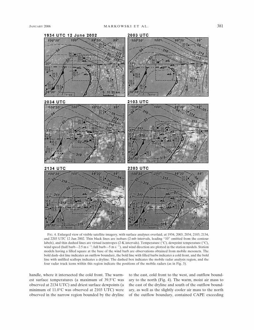
handle, where it intersected the cold front. The warm-est surface temperatures (a maximum of 39.5°C wasobserved at 2134 UTC) and driest surface dewpoints (aminimum of 11.0°C was observed at 2103 UTC) wereobserved in the narrow region bounded by the dryline

to the east, cold front to the west, and outflow bound-ary to the north (Fig. 4). The warm, moist air mass tothe east of the dryline and south of the outflow bound-ary, as well as the slightly cooler air mass to the northof the outflow boundary, contained CAPE exceeding

FIG. 4. Enlarged view of visible satellite imagery, with surface analyses overlaid, at 1934, 2003, 2034, 2103, 2134,and 2203 UTC 12 Jun 2002. Thin black lines are isobars (2-mb intervals, leading “10” omitted from the contourlabels), and thin dashed lines are virtual isentropes (2-K intervals). Temperature (°C), dewpoint temperature (°C),wind speed (half barb—2.5 m s�1; full barb—5 m s�1), and wind direction are plotted in the station models. Stationmodels having a filled square at the base of the wind barb are observations obtained from mobile mesonets. Thebold dash–dot line indicates an outflow boundary, the bold line with filled barbs indicates a cold front, and the boldline with unfilled scallops indicates a dryline. The dashed box indicates the mobile radar analysis region, and thefour radar truck icons within this region indicate the positions of the mobile radars (as in Fig. 3).


2000 J kg�1 and virtually no CIN near 2100 UTC (Fig.5).1 CAPE also was present at locations in the relativelyhot, dry low-level air mass west of the dryline and southof the outflow boundary, but a small amount (2–23 Jkg�1) of CIN was present.

A low intensified along the outflow boundary duringthe afternoon hours. Animations of reflectivity fromthe National Center for Atmospheric Research(NCAR) S-band dual-polarization Doppler radar (S-

POL; not shown), which also was situated in the easternOklahoma panhandle, depicted a spectacular cycloniccirculation about this low pressure cell. Objectivelyanalyzed equivalent reflectivity factor from the S-POLradar (Fig. 6) revealed that the mesoscale boundariesanalyzed in Figs. 3 and 4 (i.e., the dryline and outflowboundary) also were associated with reflectivity finelines.

The IHOP mobile observing facilities were deployedduring the early afternoon to northwestern Oklahomawhere the dryline and outflow boundary intersected.This area was deemed to be the most likely location forconvection initiation. Between 1934 and 2103 UTC(Fig. 4), the dryline mixed eastward, out of the IOR. In

1 Here and hereafter, CAPE and CIN were computed using themean potential temperature and specific humidity within theboundary layer, as well as virtual temperature deviations from theenvironment (Doswell and Rasmussen 1994).

FIG. 5. Skew T–logp diagrams of the soundings obtained during the 1930–2130 UTC mobile radar deployment. Isobars (solid) aredrawn at 100-mb intervals; isotherms (solid) are drawn at 10°C intervals; isentropes (solid) are drawn at 20-K intervals; pseudoadiabats(dashed) are drawn at 8°C intervals; lines of constant water vapor mixing ratio line (dashed) also are included (2, 3, 5, 8, 12, and 20 gkg�1). The locations of the rawinsondes and dropsondes are indicated in the schematic at the top right of each thermodynamic diagram.


the next 30 min, the cumulus clouds along the drylineexplosively developed into several thunderstorms (Figs.3, 4, and 6), approximately 40 km east of the center ofthe IOR, just beyond the easternmost dual-Dopplerlobes formed by the mobile radars. Damaging windsand large hail were reported in conjunction with someof the storms. Although convection initiation was notcaptured within the IOR, towering cumulus clouds—apparently indicative that plumes of air had surpassed

the LFC—developed along the outflow boundarywithin the region of dense observations between 2100and 2130 UTC (Figs. 4, 7, and 8). Curiously, this deepvertical growth occurred during the time when the out-flow boundary was accelerating southeastward throughthe IOR, apparently in response to the passage of thelow to the northeast (Fig. 4). It is the formation of thesedeep cumulus clouds that is the subject of greatest in-terest in this paper.

FIG. 6. Equivalent radar reflectivity factor recorded by the NCAR S-Pol radar at 1930, 2000, 2030, 2100, 2130,and 2200 UTC 12 Jun 2002. The dashed box indicates the mobile radar analysis region, and the four radar truckicons within this region indicate the positions of the mobile radars.


4. Boundary layer kinematic fields

a. Mesoscale boundaries

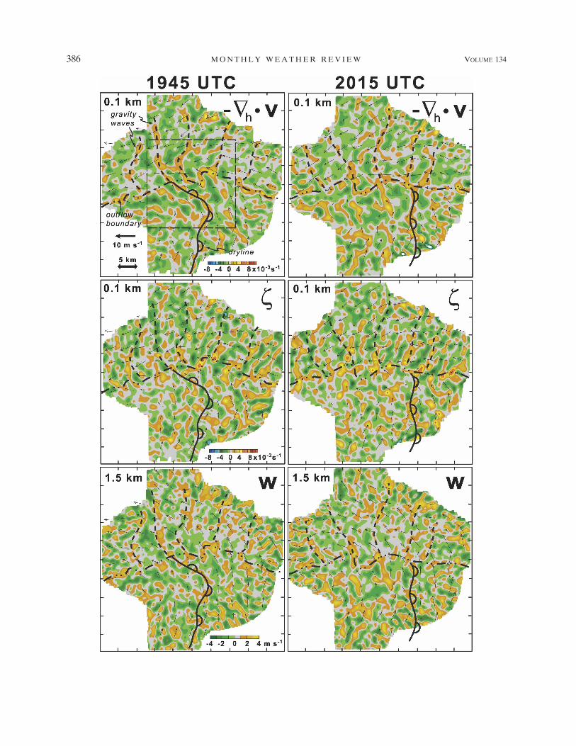
The horizontal convergence (�� · v) and verticalvorticity (�) fields at 100 m above ground level (AGL;hereafter all heights are AGL) and vertical velocity (w)at 1.5 km are displayed at 30-min intervals from 1945 to2115 UTC within the large wind synthesis domain inFigs. 9 and 10. The placement of surface boundaries isbased on the synthesized wind fields, mobile mesonetobservations (refer to Fig. 4), and radar reflectivity(e.g., Fig. 6). What is perhaps the most obvious aspectof Figs. 9 and 10 is the humbling complexity of thekinematic fields, which might tempt one to concludethat the radial velocity data were insufficientlysmoothed prior to the production of three-dimensionalwind syntheses. Yet the fields have vertical and tempo-ral continuity, which would not be anticipated in thepresence of nonmeteorological noise. For example, thetemporal autocorrelation of the vertical velocity field is�0.9 during the entire deployment (see appendix A).Although there is some artificial coupling in the vertical

introduced by the objective analysis, there is no artifi-cial coupling of fields in time. Each analysis is indepen-dent of prior and ensuing analyses. Thus, there is con-siderable confidence in the robustness of the derivedkinematic fields in Figs. 9 and 10.

Figures 9 and 10 reveal that the mesoscale bound-aries are not simply regions of quasi-two-dimensional“slabular” ascent.2 Instead, the low-level convergenceand associated vertical motion fields along the drylineand outflow boundary are highly three-dimensional,apparently the result of the superpositioning of motionsassociated with gravity waves, boundary layer convec-tive overturning, which dominates, and much weakermesoscale ascent along the dryline and outflow bound-ary. Similar along-boundary variability has been notedin past convection initiation studies (e.g., Kingsmill1995; Atkins et al. 1995), although the boundaries typi-cally have coincided with unbroken corridors of at least

2 This term has been borrowed from James and Fritsch (2003)and James et al. (2005), who used it to describe different modes ofascent within the leading updrafts of squall lines.

FIG. 7. Video frames of cloud field from CAM1 (looking north) and CAM2 (looking west) at 2015 and 2045 UTC.The locations of CAM1 and CAM2 are shown in Fig. 1. The labels reference clouds appearing in the Doppler windsyntheses displayed in Fig. 12. Clouds visible in both CAM1 and CAM2 imagery have been given the same label.


positive convergence. It is perhaps clear from visualinspection of Figs. 9 and 10 that no popular spatialaveraging technique would be capable of rendering ki-nematic fields resembling those presented in many con-ceptual models, whereby corridors of unbroken conver-gence and ascent, and enhanced relative vorticity, areassumed to be collocated with wind shift lines. Indeed,

attempts to remove the motions associated with ther-mals in order to obtain mean mesoscale motions thatresemble such conceptual models, using broader spatialfilters and time averaging (not shown), proved unsuc-cessful for this case. Conceptual models are purposelyidealized and thus greatly simplified. One worry, how-ever, is that the details excluded from previous concep-

FIG. 8. Video frames of cloud field from CAM1 (looking north) and CAM2 (looking west) at 2107, 2115, and2125 UTC. The locations of CAM1 and CAM2 are shown in Fig. 1. The labels reference clouds appearing in theDoppler wind syntheses displayed in Fig. 13. Clouds visible in both CAM1 and CAM2 imagery have been giventhe same label. The heights of some of the deep cloud tops also have been indicated.



Fig 9 live 4/C

tual models for probably well-intentioned reasons mayvery well turn out to be crucial in addressing outstand-ing questions pertaining to convection initiation. Thismatter will be discussed in greater detail in section 7.Since observations having the spatial and temporalresolution of those presented herein are rare, some un-avoidable uncertainty exists as to the generality of ourobservations.

Boundary layer convection dominates the kinematicfields on both sides of the dryline and outflow bound-ary. There is a mild suggestion of organization into rollsand cells, especially on the warm side of the outflowboundary, although not to the degree documented byWeckwerth et al. (1997). Maximum vertical velocitymagnitudes at 1.5 km are approximately 4 m s�1 on thewarm side of the outflow boundary and approximately3 m s�1 on the cool side of the outflow boundary. Up-drafts tend to be associated with relative maxima inradar reflectivity factor (linear correlation coefficientswere �0.4 during the deployment),3 probably as a re-sult of insect lofting (Wilson et al. 1994). Along whathave been referred to as mesoscale boundaries (i.e., thedryline and outflow boundary), there is no outstandingenhancement of upward vertical velocities, althoughthis does not necessarily imply that the characteristicsof air parcel trajectories are similar along and awayfrom the boundaries, as will be discussed later.

b. Gravity waves

Gravity waves are readily apparent north of the out-flow boundary in the radar reflectivity data [e.g., Fig. 6(particularly the 1930–2030 UTC panels)] and in theretrieved perturbation pressure fields near the surface(Fig. 11). The oscillation of the horizontal wind vectorfield throughout the boundary layer due to the passageof the wave fronts is very evident in animations (notshown). The waves are not easily discernible in the ra-dar reflectivity data nor the low-level pressure field af-ter approximately 2100 UTC. This case nicely demon-strates that the influence of gravity waves can extendinto a neutrally stratified, convective boundary layer.

The wavelength of the waves averages approximately10 km and the motion was toward the west at approxi-mately 4 m s�1. Soundings indicate a neutrally stratifiedboundary layer on the cool side of the outflow bound-ary, capped by a stable layer between approximately700 and 800 mb (Fig. 5). The zonal wind speed in thestable layer has a westerly component; thus, the waveshave a westward propagation. In the underlying neu-trally stable boundary layer of the outflow air mass,however, the zonal wind speed is easterly, averaging5–6 m s�1. Thus, the boundary layer updrafts associatedwith the waves are located roughly a quarter-wavelength west (downstream) of the pressure troughs(Fig. 11). The vertical velocity field, however, is per-haps less orderly (i.e., far from being quasi-two-dimensional) than one might expect in the presence ofgravity waves. This probably is a result of the interac-tion of the gravity wave motions with convective cells.

c. Vertical vorticity extrema

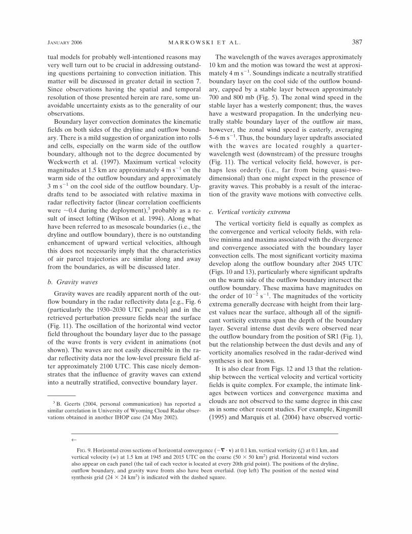
The vertical vorticity field is equally as complex asthe convergence and vertical velocity fields, with rela-tive minima and maxima associated with the divergenceand convergence associated with the boundary layerconvection cells. The most significant vorticity maximadevelop along the outflow boundary after 2045 UTC(Figs. 10 and 13), particularly where significant updraftson the warm side of the outflow boundary intersect theoutflow boundary. These maxima have magnitudes onthe order of 10�2 s�1. The magnitudes of the vorticityextrema generally decrease with height from their larg-est values near the surface, although all of the signifi-cant vorticity extrema span the depth of the boundarylayer. Several intense dust devils were observed nearthe outflow boundary from the position of SR1 (Fig. 1),but the relationship between the dust devils and any ofvorticity anomalies resolved in the radar-derived windsyntheses is not known.

It is also clear from Figs. 12 and 13 that the relation-ship between the vertical velocity and vertical vorticityfields is quite complex. For example, the intimate link-ages between vortices and convergence maxima andclouds are not observed to the same degree in this caseas in some other recent studies. For example, Kingsmill(1995) and Marquis et al. (2004) have observed vortic-

3 B. Geerts (2004, personal communication) has reported asimilar correlation in University of Wyoming Cloud Radar obser-vations obtained in another IHOP case (24 May 2002).

←

FIG. 9. Horizontal cross sections of horizontal convergence (�� · v) at 0.1 km, vertical vorticity (�) at 0.1 km, andvertical velocity (w) at 1.5 km at 1945 and 2015 UTC on the coarse (50 � 50 km2) grid. Horizontal wind vectorsalso appear on each panel (the tail of each vector is located at every 20th grid point). The positions of the dryline,outflow boundary, and gravity wave fronts also have been overlaid. (top left) The position of the nested windsynthesis grid (24 � 24 km2) is indicated with the dashed square.


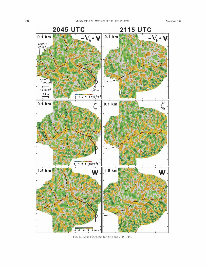
FIG. 10. As in Fig. 9, but for 2045 and 2115 UTC.


Fig 10 live 4/C

ity maxima along mesoscale boundaries separated by awell-defined wavelength, with local enhancements ofhorizontal convergence located roughly a quarter-wavelength downstream of the vorticity maxima, ap-parently due to the interaction of the vortices with thewind shift lines. It may be that the processes governingthe development of the vortices observed in this casediffer from those operating in the past studies cited. Adetailed analysis of the evolution and dynamics of theboundary layer vortices is beyond the scope of thepresent study; however, such an investigation is pro-vided by Markowski and Hannon (2006).

5. Relationship between kinematic andthermodynamic fields

The near-ground buoyancy gradient along the out-flow boundary is notably weak throughout the data col-lection period, largely as a result of larger moistureconcentrations on the cool side of the boundary (Fig.4). The virtual potential temperature gradient mea-sured at the surface by the mobile mesonets is approxi-mately 1 K (10 km)�1 at the surface within the IOR(Fig. 4). The retrieved virtual potential temperaturegradient at 0.1 km is even weaker (e.g., Fig. 14), withslightly more buoyant air north of the outflow boundaryat times (e.g., Fig. 14). These retrieval results, althoughsurprising, are supported by sounding observations

(e.g., compare the nearly simultaneous 1933 and 1934UTC soundings obtained on opposite sides of the out-flow boundary in Fig. 5, whereby the surface tempera-tures are similar but the specific humidity is �4 g kg�1

larger on the sounding north of the boundary). Therealso is some suggestion from the soundings (Fig. 5) thatthe lapse rates north of the outflow boundary had agreater tendency to be superadiabatic within the sur-face layer. This effect also would reduce the near-ground buoyancy gradient across the outflow bound-ary.

A larger buoyancy gradient is present across the out-flow boundary in the middle to upper portions of theboundary layer (Fig. 14), although even here the gra-dient is relatively modest by mesoscale standards [gen-erally less than 1 K (5 km)�1]. In section 7 we discussthe possibility that the absence of a horizontally con-tiguous, unbroken slab of mesoscale ascent along theoutflow boundary may be related to the weak baroc-linity along the boundary.

South of the outflow boundary, in situ data from air-craft flying between 0.4 and 0.7 km, not surprisingly,reveal that updrafts tend to be collocated with virtualpotential temperature excesses (Fig. 15, top). Further-more, boundary layer updrafts also tend to be situatedabove regions of virtual potential temperature excess atthe surface, as evidenced by mobile mesonet observa-tions (Fig. 16). In contrast, the correlation between up-

FIG. 11. Perturbation pressure fields at 0.1 km at (left) 2015 and (right) 2045 UTC within the 24 � 24 km2 windsynthesis domain (see Fig. 9). Contours have been drawn at 0.04-mb intervals. Negative contours are dashed. Theperturbations are with respect to the domain-averaged pressure perturbation at 0.1 km. Vertical velocities greaterthan 0.5 m s�1 at 1.5 km have been shaded gray. The outflow boundary is depicted using the same symbology asin Fig. 3, and phase fronts have been drawn through pressure troughs using dashed lines.


drafts (Fig. 12 and 13) and retrieved positive buoyancyanomalies (Fig. 14) is relatively small in the middle toupper boundary layer. Perhaps this observation ispartly a result of the buoyancy fields necessarily havingbeen smoothed to a greater degree than the verticalvelocity fields, or perhaps the updrafts simply are not

positively buoyant more than approximately a kilome-ter above the ground. North of the outflow boundary,the relationship between buoyancy and vertical velocityis ill defined at all levels (Fig. 15, bottom), perhapsowing to the influence of gravity wave dynamics.

The in situ aircraft data also reveal that boundary

FIG. 12. Horizontal cross sections of the (left) vertical velocity (w) field at 1.5 km and (right) vertical vorticity(�) field at 0.1 km within the 24 � 24 km2 wind synthesis domain (see Fig. 9) at 2015 and 2045 UTC. Horizontalwind vectors at 1.5 and 0.1 km also are displayed in the vertical velocity and vertical vorticity panels, respectively(see scale in upper-left panel). The outflow boundary is depicted using the same symbology as in Fig. 3. Gravitywave phase fronts have been drawn through pressure troughs as in Fig. 11. Cloud positions determined fromphotogrammetry are shaded gray, and some of the clouds appearing in Fig. 7 have been labeled with the lettersA–H. The locations and fields of view of the two cameras used for the photogrammetric cloud analysis areindicated in the left panels. The contours depicting the w field at 1.5 km are drawn at 1 m s�1 intervals, with positive(negative) contours drawn as solid (dashed) lines and the 0 m s�1 contour suppressed. The contours depicting the� field at 0.1 km are drawn at 2 � 10�3 s�1 intervals, with positive (negative) contours drawn as solid (dashed) linesand the 0 s�1 contour suppressed.


FIG. 13. As in Fig. 12, but for 2107, 2115, and 2125 UTC. Some of the clouds appearing in Fig. 8 havebeen labeled with the letters A–H. The “U” label indicates the updraft referred to in Fig. 17. The flighttrack of the NRL P-3 aircraft also is indicated (tick marks are at 1-min intervals).


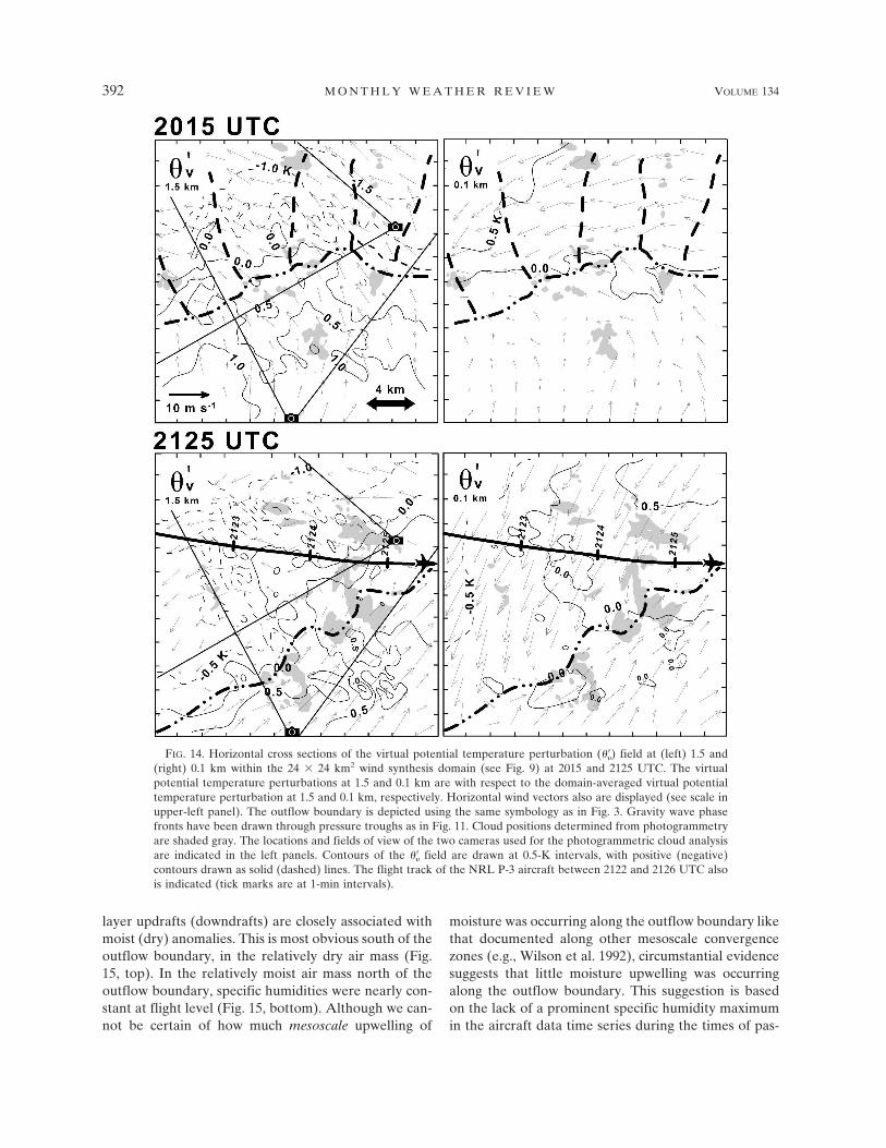
layer updrafts (downdrafts) are closely associated withmoist (dry) anomalies. This is most obvious south of theoutflow boundary, in the relatively dry air mass (Fig.15, top). In the relatively moist air mass north of theoutflow boundary, specific humidities were nearly con-stant at flight level (Fig. 15, bottom). Although we can-not be certain of how much mesoscale upwelling of

moisture was occurring along the outflow boundary likethat documented along other mesoscale convergencezones (e.g., Wilson et al. 1992), circumstantial evidencesuggests that little moisture upwelling was occurringalong the outflow boundary. This suggestion is basedon the lack of a prominent specific humidity maximumin the aircraft data time series during the times of pas-

FIG. 14. Horizontal cross sections of the virtual potential temperature perturbation (��) field at (left) 1.5 and(right) 0.1 km within the 24 � 24 km2 wind synthesis domain (see Fig. 9) at 2015 and 2125 UTC. The virtualpotential temperature perturbations at 1.5 and 0.1 km are with respect to the domain-averaged virtual potentialtemperature perturbation at 1.5 and 0.1 km, respectively. Horizontal wind vectors also are displayed (see scale inupper-left panel). The outflow boundary is depicted using the same symbology as in Fig. 3. Gravity wave phasefronts have been drawn through pressure troughs as in Fig. 11. Cloud positions determined from photogrammetryare shaded gray. The locations and fields of view of the two cameras used for the photogrammetric cloud analysisare indicated in the left panels. Contours of the �� field are drawn at 0.5-K intervals, with positive (negative)contours drawn as solid (dashed) lines. The flight track of the NRL P-3 aircraft between 2122 and 2126 UTC alsois indicated (tick marks are at 1-min intervals).


sage through the outflow boundary (e.g., Fig. 15), andthe lack of a persistent, spatially continuous corridor ofstrong convergence along the outflow boundary.

6. Relationships between cumulus clouddevelopment and boundary layer kinematic andthermodynamic fields

Shallow cumulus clouds were observed in the IORthroughout the deployment from 1930 to 2130 UTC(Figs. 7 and 8). Between 2100 and 2130 UTC, some ofthe clouds grew to more significant depths (Figs. 4 and

8). Photogrammetric cloud analyses indicated that thetops of the tallest clouds in the IOR exceeded 7 kmduring this period. Below we provide a discussion of therelationships between kinematic and thermodynamicboundary layer structures and cloud formation. Em-phasis is placed on the development of the deepestclouds in the IOR after 2100 UTC.

a. Shallow cumulus cloud development prior to2100 UTC

As one would probably anticipate, the area occupiedby cumulus clouds was much smaller than the area oc-cupied by updrafts (Fig. 12). Not all updrafts were as-sociated with cumulus clouds, and where they were, theclouds spanned smaller horizontal scales than their par-ent updrafts. These observations are likely indicative ofentrainment and moisture heterogeneity. Clouds gen-erally were situated above updrafts, although someclouds were observed in regions of nearly zero orslightly negative vertical velocity (e.g., the clouds near“A” and south of “D” at 2045 UTC; Fig. 12). The latter,however, were situated in regions where updrafts hadbeen present 5–10 min earlier; that is, cumulus cloudsnot located within updrafts were at least observed to belocated within regions having histories of ascent.

Cumulus cloud development was not enhanced alongthe outflow boundary. The clouds grew in numbergradually during the deployment throughout the entireIOR (Figs. 7 and 12). Cloud bases were determinedfrom photogrammetry to range from 1.6 to 2.5 km, withlower (higher) cloud bases observed north (south) ofthe outflow boundary where the relative humidity waslarger (smaller). Thus, the cloud bases were roughly0.1–1.0 km above the level at which vertical velocityfields are displayed in Figs. 12, 13, and 14.

FIG. 15. Time series of virtual potential temperature (��; solid,black) and specific humidity (q; solid, gray) from the NRL P-3aircraft from (top) 2106:25–2109:55 and (bottom) 2122:10–2125:40UTC. The synthesized vertical velocity (w; dashed; black) inter-polated to the aircraft position also is overlaid. Aircraft data weresmoothed with a 10-s running mean filter. The flight level was atapproximately 0.6 km AGL for both time periods. The abscissa islabeled with both x-grid coordinate and UTC time. The flighttracks also are overlaid in Figs. 14 and 13.

FIG. 16. Time series of mobile mesonet (“probe 6”) virtual po-tential temperature (��; solid) at 3 m AGL vs synthesized verticalvelocity (w; dashed) at 1.5 km AGL from 2100 to 2130 UTC. Themobile mesonet data were smoothed with a 12-s running meanfilter.


b. Deep cumulus cloud development between 2100and 2130 UTC

Cumulus clouds continued to increase in number af-ter 2100 UTC, and several of these grew to heights wellabove the LFC (e.g., cloud “F” in Fig. 8 reached analtitude of 7.2 km at 2125 UTC). Although shallow cu-mulus cloud development was not confined to the out-flow boundary, deep cumulus cloud development wasobserved almost exclusively along the outflow boundary(Figs. 8 and 13). Interestingly, vertical velocities withinthe boundary layer were no larger beneath the deepestcumulus clouds than they were beneath the shallow cu-mulus clouds. For example, between 2107 and 2125UTC, updrafts exceeding 3 m s�1 were observed at anelevation of 1.5 km on both sides of the outflow bound-ary (Fig. 13), and as documented in section 4, the out-flow boundary was not a region of spatially continuous,enhanced vertical velocity (Figs. 9 and 10). The deepestcloud at 2115 (labeled as “E” in Fig. 8) and 2125 UTC(labeled as “F” in Fig. 8) is situated above 1–2 m s�1

updrafts at 1.5 km, whereas updrafts as strong as 3–4m s�1 frequently were associated with clear skies oronly shallow cumulus development, especially in thewarm sector south of the outflow boundary.

Trajectories into shallow and deep cumulus cloudswere compared in an attempt to understand why thedevelopment of deep cumulus clouds was confined tothe outflow boundary despite the fact that there was noapparent enhancement of vertical velocities along theoutflow boundary. Trajectories were computed usingtrilinear spatial interpolation and a fourth-orderRunge–Kutta time integration algorithm using a timestep of 10 s. The three-dimensional wind fields wereassumed to vary linearly in time between the twoDoppler analyses closest to the current time of a pointalong a trajectory. An error analysis of the trajectoriesis presented in appendix B.

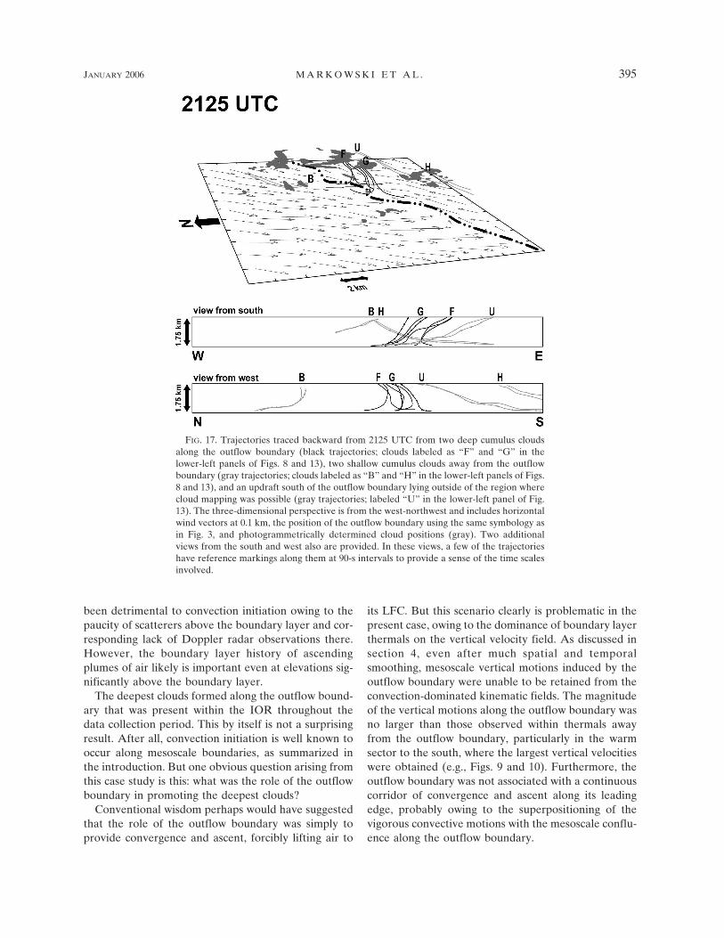
Backward trajectories originating from clouds B, F,G, and H at 2125 UTC are displayed in Fig. 17. Thecloud bases range from 1.7 to 2.1 km; thus, the basesgenerally are located slightly above the level where tra-jectories originate (1.7 km, the highest level deemed tohave reliable wind velocity fields). The top of cloud Fwas 7.2 km at 2125 UTC, and cloud G grew to a similarheight shortly after 2125 UTC (Fig. 8). Clouds F and Gwere located along the outflow boundary (Fig. 13).Clouds B and H were shallow cumulus clouds that de-veloped several kilometers north and south of the out-flow boundary, respectively (Fig. 13). Trajectories en-tering the strong updraft (�4 m s�1 at 1.5 km) �5 kmsoutheast of cloud G (labeled “U” in Fig. 13) also wereexamined. It is not known whether this updraft was

associated with shallow cumulus development or no cu-mulus development because the updraft was not withinthe field of view of either CAM1 or CAM2. It is onlyknown that this updraft was not associated with deepcumulus cloud formation.

The most obvious difference in the trajectories en-tering the deep clouds along the outflow boundary ver-sus those entering the shallow clouds that formed awayfrom the boundary is the slope of the trajectories (Fig.17). The trajectories entering the deep clouds along theoutflow boundary were much more vertical than thoseentering the shallow clouds away from the boundary.The more upright trajectories along the boundary werea result of the relative minimum in both horizontal windspeed (Fig. 10) and vertical wind shear along theboundary (Fig. 18). Indeed, updrafts along the bound-ary were more erect than those away from the bound-ary.

The differences in the updraft and trajectory slopesmay imply differences in the dilution of buoyancy andreduction of potential buoyancy (a function of equiva-lent potential temperature, �e) for vertical excursionsoccurring along and away from the outflow boundary.The highly elongated, gently sloped excursions occur-ring away from the boundary are perhaps more suscep-tible to the detrimental effects of entrainment. Severalsoundings south of the outflow boundary (most notablythe 2046 and 2059 UTC soundings; Fig. 5) indicatedthat the moisture concentration was not constant withheight, but rather there was a decrease of 1–2 g kg�1

between the surface and the top of the boundary layer;thus, entrainment en route to the cloud base wouldhave resulted in a reduction of potential buoyancy. Fur-thermore, in the 2115 and 2125 UTC analyses, the basesof the clouds developing along the outflow boundarytended to be wider than those that developed awayfrom the outflow boundary (Fig. 13); this observationmight be indirect evidence of less entrainment alongthe trajectories entering the clouds that developedalong the outflow boundary. Additional discussion fol-lows in the next section.

7. Comments on convection initiation

a. Role of the outflow boundary in enabling deepcumulus cloud development

Although this case has been regarded as an exampleof convection initiation “failure,” some aspects prob-ably are similar to those present in “success” cases. Forexample, although no precipitating convection devel-oped within the IOR, some plumes of air did in factattain their LFC. We are unable to address what pro-cesses occurring above the boundary layer might have


been detrimental to convection initiation owing to thepaucity of scatterers above the boundary layer and cor-responding lack of Doppler radar observations there.However, the boundary layer history of ascendingplumes of air likely is important even at elevations sig-nificantly above the boundary layer.

The deepest clouds formed along the outflow bound-ary that was present within the IOR throughout thedata collection period. This by itself is not a surprisingresult. After all, convection initiation is well known tooccur along mesoscale boundaries, as summarized inthe introduction. But one obvious question arising fromthis case study is this: what was the role of the outflowboundary in promoting the deepest clouds?

Conventional wisdom perhaps would have suggestedthat the role of the outflow boundary was simply toprovide convergence and ascent, forcibly lifting air to

its LFC. But this scenario clearly is problematic in thepresent case, owing to the dominance of boundary layerthermals on the vertical velocity field. As discussed insection 4, even after much spatial and temporalsmoothing, mesoscale vertical motions induced by theoutflow boundary were unable to be retained from theconvection-dominated kinematic fields. The magnitudeof the vertical motions along the outflow boundary wasno larger than those observed within thermals awayfrom the outflow boundary, particularly in the warmsector to the south, where the largest vertical velocitieswere obtained (e.g., Figs. 9 and 10). Furthermore, theoutflow boundary was not associated with a continuouscorridor of convergence and ascent along its leadingedge, probably owing to the superpositioning of thevigorous convective motions with the mesoscale conflu-ence along the outflow boundary.

FIG. 17. Trajectories traced backward from 2125 UTC from two deep cumulus cloudsalong the outflow boundary (black trajectories; clouds labeled as “F” and “G” in thelower-left panels of Figs. 8 and 13), two shallow cumulus clouds away from the outflowboundary (gray trajectories; clouds labeled as “B” and “H” in the lower-left panels of Figs.8 and 13), and an updraft south of the outflow boundary lying outside of the region wherecloud mapping was possible (gray trajectories; labeled “U” in the lower-left panel of Fig.13). The three-dimensional perspective is from the west-northwest and includes horizontalwind vectors at 0.1 km, the position of the outflow boundary using the same symbology asin Fig. 3, and photogrammetrically determined cloud positions (gray). Two additionalviews from the south and west also are provided. In these views, a few of the trajectorieshave reference markings along them at 90-s intervals to provide a sense of the time scalesinvolved.


Another reasonable a priori hypothesis for the roleof the outflow boundary in promoting the deepest cu-mulus clouds might have been mesoscale moisture up-welling along the boundary. Such upwelling (e.g., Wil-son et al. 1992) could have promoted convection initia-tion by deepening the moist layer, thereby reducing theamount of �e dilution resulting from entrainment withinrising plumes of air. The data that could reveal such amoisture enhancement in the 12 June 2002 case arelimited; for example, only two aircraft passages throughor along the outflow boundary occurred during the2100–2130 UTC time period. But for the limitedamount of data that do exist, no evidence could befound suggesting a local deepening of the moist layer inthe vicinity of the outflow boundary. As discussed insection 5, in situ data from the aircraft failed to reveala prominent specific humidity maximum along the out-flow boundary (Fig. 15). The inability to observe amoisture enhancement along the outflow boundarymight be consistent with the lack of a persistent, spa-tially continuous corridor of strong convergence.

In the previous section, profound differences werenoted between the trajectories entering the deep cumu-lus clouds along the outflow boundary and those enter-ing the shallow cumulus clouds away from the outflowboundary (Fig. 17), with the former trajectories (andtheir associated updrafts) being more vertical than the

latter. The differences in updraft slope imply differ-ences in the magnitude of entrainment along the tra-jectories (e.g., Weisman 1992). In addition to the obvi-ous differences in cloud depth along the outflow bound-ary versus away from it, the cloud width was enhancedalong the outflow boundary (e.g., the 2115 and 2125UTC panels of Fig. 13), which might be circumstantialevidence of reduced �e dilution within the rising plumesalong the outflow boundary.

The above observations lead us to hypothesize thatthe role of outflow boundary in promoting the deepestcumulus clouds in this case was not related to enhancedvertical velocities or mesoscale moisture upwelling. In-stead, we hypothesize that the role of outflow boundarymight only have been to promote updrafts that were lesssusceptible to �e dilution (Fig. 19). This scenario differssomewhat from that illustrated by Crook (1996) andCrook and Klemp (2000), who showed that vertical ex-cursions could be dynamically enhanced when the flowand shear above a convergence line is decreased, ratherthan “thermodynamically enhanced” via reducing en-trainment, which is what is being proposed here. Ourfindings also might suggest some applicability to con-vection initiation of the theory presented by Rotunnoet al. (1988), which relates the slope of the updraftalong the leading edge of a density current to the mag-nitudes of the density excess and ambient wind shear.

If entrainment more adversely affected rising plumesof air away from the outflow boundary than along theoutflow boundary, one might reasonably ask why ver-tical velocities along the outflow boundary would notbe larger than those away from the outflow boundary.

FIG. 18. Vertical wind shear vectors between 1.5 and 0.1 km (v1.5

km � v0.1 km) within the 24 � 24 km2 wind synthesis domain (seeFig. 9). Photogrammetrically determined cloud positions areshaded gray.

FIG. 19. Idealization of the trajectories into the shallow anddeep cumulus clouds observed away from and along the outflowboundary, respectively. Away from the outflow boundary, thetrajectories into the shallow cumulus clouds significantly departfrom the vertical. Along the outflow boundary, the trajectoriesinto the deep cumulus clouds are much more vertical owing to therelative minimum in horizontal wind speed and vertical windshear present along the boundary. The differences in the trajec-tory slopes, which also were a manifestation of differences in theslopes of the updrafts in this case, may imply differences in thedilution of buoyancy and potential buoyancy (a function ofequivalent potential temperature) for vertical excursions occur-ring along and away from the mesoscale boundary.


The vertical velocity fields synthesized in this study allare located below the lifting condensation level (LCL),where soundings revealed that potential temperaturewas constant with height within the IOR (at least abovethe surface layer); however, many soundings also re-vealed that specific humidity decreased by 1–2 g kg�1

from the surface to the top of the boundary layer (Fig.5). Given these thermodynamic profiles below theLCL, entrainment would reduce the specific humiditybut not the potential temperature, and because buoy-ancy is much more strongly a function of potential tem-perature, vertical velocities below the LCL would notbe affected significantly by the entrainment of slightlydrier air. However, the reduction of �e below the LCLcorresponds to a reduction of the potential buoyancyand vertical velocity that can be realized above the LCLand LFC, since the magnitude of the buoyancy in adeep cumulus cloud depends in large part on the mag-nitude of the latent heat release. Thus, vertical veloci-ties above the LCL (and cloud depths) might be antic-ipated to be more adversely affected than vertical ve-locities below the LCL by �e dilution occurring belowthe LCL. In reference to the opening paragraph of thissection, it is in this way that the boundary layer historyof ascending plumes can be important even at eleva-tions significantly above the boundary layer.

The above thermodynamic arguments regarding en-trainment do not consider the entrainment of momen-tum, which would weaken updrafts regardless of theimpact of entrainment on buoyancy. South (on thewarm side) of the outflow boundary, where vertical ve-locities were as strong or even occasionally strongerthan along the outflow boundary, it is possible that thethermals originating at the surface were subjected to alarger initial buoyancy force, thereby offsetting themore significant momentum entrainment.

b. The failure of convection initiation

A major challenge we face in this study is that it is notpossible to know how the atmosphere would haveevolved had the processes observed in this case notbeen operating. This is the inherent difficulty in ana-lyzing null cases, which is probably one reason whyrelatively few are documented in the literature(Doswell et al. 2002)—at least a disproportionate num-ber of cases when one considers the fact that convectionfails to develop over far more regions than it does de-velop over. The best we can do is document recurringprocesses and environmental characteristics present innull cases that are absent in “success” cases, in order todetermine the conditions that promote convection ini-tiation.

One aspect of this case that might have been unfa-

vorable for convection initiation along the outflowboundary is the aforementioned absence of a continu-ous, persistent corridor of convergence. This finding issimilar to that made by Arnott et al. (2004) in anotherIHOP case (10 June 2002) along a segment of a coldfront where deep convection failed to be initiated. Inpast studies documenting convection initiation “suc-cesses,” although significant along-line variability occa-sionally was observed, the mesoscale boundaries towhich convection initiation was attributed coincidedwith unbroken or nearly unbroken corridors of conver-gence and updraft (e.g., Kingsmill 1995; Atkins et al.1995; Richardson et al. 2004).

In section 5 the possibility was raised as to whetherthe lack of a horizontally contiguous, unbroken slab ofmesoscale ascent along the outflow boundary was re-lated to the weak baroclinity along the boundary. In-deed, Arnott et al. (2004) and Stonitsch and Markowski(2004) have found a strong relationship between baro-clinity and the organization of the vertical motion field(i.e., its horizontal continuity) along mesoscale bound-aries in other IHOP cases. These studies suggest thatthe organization of the vertical motion field along me-soscale boundaries depends on the relative significanceof density current or frontal dynamics compared to mo-tions associated with thermals, with the vertical motionfield along boundaries becoming increasingly “slabu-lar” as density current or frontal dynamics becomemore dominant.

One also might wonder why a radar reflectivity fineline would be observed in conjunction with a mesoscaleboundary along which a spatially continuous corridor ofconvergence is absent (Fig. 6), but the fine line wasrelatively diffuse. A well-defined convergence zonealso was absent along the dryline during the periodwhen the dryline was sampled by the ground-based ra-dars, but we cannot comment on the kinematic struc-ture of the dryline at the time when thunderstormswere initiated east of the IOR. It may be noteworthythat the fine line associated with the dryline becamemuch more prominent east of the IOR near the time ofconvection initiation (see 2100 UTC panel of Fig. 6).

The soundings obtained in the IOR in the vicinity ofthe outflow boundary near the time when deep cumulusclouds developed (e.g., the 2046 and 2059 UTC sound-ings; Fig. 5) do not suggest the same magnitude of me-soscale ascent and moist layer deepening as the sound-ing near the location of convection initiation farthereast (e.g., the 2056 UTC sounding; Fig. 5). The lattersounding has virtually no CIN, whereas the formersoundings have a modest amount of CIN (�20 J kg�1),unless CIN is computed assuming undiluted ascent orby lifting a parcel originating in the superadiabatic con-


tact layer. It is possible that the previously cited pro-motion of “�e dilution-resistant” updrafts along the out-flow boundary was sufficient for the development ofdeep cumulus clouds, but that �e dilution was not en-tirely absent owing to the lack of moisture upwelling sothat there simply was not enough potential buoyancyremaining once the LFC was achieved in order to sup-port precipitating cumulonimbus clouds. Unfortu-nately, no soundings were obtained in close proximityto the deep cumulus clouds along the outflow boundaryduring the 2100–2130 UTC period.

c. Conceptual models of convection initiation

One critical issue seems to be related to the super-positioning of motions induced by mesoscale dynamics(e.g., density current dynamics, which has been invokedin theoretical studies of outflows and drylines) and mo-tions associated with the ubiquitous buoyant convec-tion in the boundary layer. How are their relative con-tributions to the vertical motion field affected by thebaroclinity present along the mesoscale boundaries?Do the relative contributions mostly impact the magni-tude of the vertical motions or the spatial patterns ofthe vertical motions, and what are the consequences forparcel trajectories in the vicinity of mesoscale bound-aries?

As already noted numerous times throughout,boundary layer thermals dominated the horizontal con-vergence and vertical motion fields in this case, and it islikely that they would be equally as dominant or at leastassume first-order importance in most warm-seasonconvection initiation cases. Many past conceptual mod-els of convection initiation have been based on meso-scale dynamics, and many of these models are two-dimensional. From the perspective of mesoscale dy-namics and convection initiation, thermals often areregarded as noise and are excluded from such models.This approach is certainly understandable—after all,much convection initiation forecasting success can berealized simply by identifying mesoscale or synoptic-scale wind shifts or radar fine lines. But the present casestrongly suggests that advances made in our conceptualmodels of convection initiation should include a promi-nent role for boundary layer convection in addition tomesoscale boundaries. This fundamentally requiresthree-dimensionality. Even when a quasi-two-dimensional mesoscale boundary is present, significantalong-boundary heterogeneity is guaranteed in thepresence of boundary layer convection. This point alsohas been raised by some previous studies; for example,Atkins et al. (1995) presented a conceptual model inwhich the deepest cumulus clouds were initiated at theintersections of convective rolls with a sea-breeze front.

The possible importance of vortices along boundariesin convection initiation also has been raised by manyinvestigators (e.g., Kingsmill 1995; Kanak et al. 2000;Lee and Finley 2000; Marquis et al. 2004, among oth-ers), and the development and evolution of such vorti-ces may be closely connected to boundary layer con-vection (e.g., Shapiro and Kanak 2002), and perhapsthe interaction of convective cells or rolls with meso-scale boundaries (e.g., Atkins et al. 1995). We speculatethat the complex superpositioning of boundary layerthermals and mesoscale motions are probably why de-termining precisely where convection initiation will oc-cur has been so difficult, even along well-defined me-soscale boundaries.

8. Summary and conclusions

This paper has examined the kinematic and thermo-dynamic structure of the boundary layer in the vicinityof an outflow boundary and dryline on 12 June 2002,processes associated with the development of both shal-low and deep cumulus clouds, and processes that mayhave contributed to the failure of the initiation of sus-tained, precipitating cumulonimbus clouds. The obser-vations presented herein permit the following conclu-sions pertaining to this study:

• The convergence and vertical motion fields weredominated by motions associated with boundarylayer thermals rather than dynamics associated withthe mesoscale boundaries.

• The influence of internal gravity waves propagatingthrough a statically stable layer capping the boundarylayer can extend throughout the underlying neutrallystratified boundary layer.

• The deepest cumulus clouds occurring within the re-gion of intensive observations developed along anoutflow boundary, where trajectories into the cloudswere nearly vertical; shallow cumulus clouds devel-oped away from this outflow boundary, where verti-cal velocities were equally as large but trajectorieswere much more inclined from the vertical.

The final conclusions are more tentative:

• The role of the outflow boundary in enabling deepcumulus cloud development was to promote updraftsin proximity to the boundary that were less suscep-tible to �e dilution, rather than to provide enhancedvertical velocities or a region of persistent mesoscaleconvergence within which moisture upwelling oc-curred.

• The lack of a persistent, spatially continuous corridorof mesoscale ascent along the outflow boundary andassociated moisture upwelling contributed to convec-tion initiation failure along the outflow boundary.


Uncertainties regarding the generality of findings madefrom single case studies are unavoidable. We cannotsay whether our hypothesized role for the outflowboundary in the convection initiation process would ap-ply to a large number of other cases involving meso-scale boundaries. For example, in this case, the outflowboundary was associated with only weak baroclinity,and boundary layer thermals were notably vigorous. Itis quite possible, perhaps even likely, that the dynamicsdirectly associated with mesoscale boundaries assumegreater prominence when the boundary layer kinematicfields are less dominated by thermals or when the me-soscale boundaries are associated with more substantialbaroclinity. Nonetheless, we believe that our proposedand previously unconsidered role of mesoscale bound-aries in promoting deep cloud formation to be worthyof further scrutiny in additional case studies.

We also would encourage additional study of the re-lationship between radar reflectivity fine lines and thevertical velocity field. Reflectivity fine lines may be thebest way of inferring the presence of vertical motion orits history in real time. But it is precisely because radarreflectivity may be a better indicator of updraft historyrather than instantaneous vertical velocity that makesthis topic worthy of additional attention. We also be-lieve that it would be extremely worthwhile to furtherexplore how gravity waves and mesoscale boundariesinteract with convective boundary layers. Finally, therelationships between the vertical velocity and verticalvorticity fields received only superficial treatment. Amuch more thorough investigation of the nature of vor-tices, their evolution, forcings, and intricate feedbacksto vertical motion, and possible convection initiationramifications are presented in a companion paper(Markowski and Hannon 2006).

Acknowledgments. We wish to thank Drs. Yvette Ri-chardson, John Clark, Josh Wurman, Erik Rasmussen,Conrad Ziegler, Bart Geerts, and Tammy Weckwerthfor many fruitful discussions over the course of thiswork, and Dr. Manos Anagnostou, Dr. Kevin Knupp,and Justin Walters for providing XPOL radar data and(University of Alabama in Huntsville) Mobile Inte-grated Profiling System (MIPS) data. We also receivedinvaluable assistance from Dr. Jerry Guynes, Curtis Al-exander, Mike Buban, Steve Williams, Marisa Ferger,and particularly Nettie Arnott, who graciously allowedus to use her advection correction program and otherDOW postprocessing programs. IHOP could not haveoccurred without the leadership and devotion of Drs.David Parsons and Tammy Weckwerth, the dedicationof the Joint Office of Science Support, and all of thestudent participants who spent countless hours collect-

ing data in the field. Software developed by NCAR washeavily used in this work. Radar editing was performedusing SOLO, objective analyses of radar data were pro-duced by REORDER, and wind syntheses were pro-duced by CEDRIC. This research was supported byNational Science Foundation Grant ATM-0130307made to Pennsylvania State University.

APPENDIX A

Wind Synthesis Sensitivity Analysis

A number of sensitivity tests were undertaken to ex-amine the robustness of the three-dimensional windsyntheses. In this appendix, the effects of radar azimutherrors, objective analysis parameters, and advection ve-locity on the wind syntheses are assessed. Trajectoryuncertainties also are investigated.

a. Azimuth errors

Prior to the interpolation of radar data to a Cartesiangrid, it is imperative that the orientation of the radar isaccurately known. This orientation can be determinedby identifying landmarks in the ground clutter patternwhose positions are known, or by scanning the sun (itsposition is well established from astronomical tables),as already discussed. All orientation uncertainty typi-cally cannot be eliminated, especially when identifyingground clutter targets, owing to a finite beamwidth andpossible uncertainties in the reported positions of thelandmarks. The impact of azimuth errors on the inter-polation and subsequent wind synthesis ultimately de-pend on the azimuthal radial velocity gradients, whichare range and weather dependent.

To quantify the propagation of azimuth angle errorsinto the wind syntheses, radial velocity data from eachof the four mobile radars were rotated by 1° (roughly afull half-power beamwidth) at five randomly selectedanalysis times. The rotations were made in both thecounterclockwise and clockwise direction in order todetermine the largest effect on the wind syntheses. It isbelieved that this approach represents a “worst case”scenario—it is very unlikely that all four radars wouldhave been incorrectly oriented by a full degree of azi-muth. The largest rms error (smallest linear correlationcoefficient) in the vertical velocity field for five ran-domly chosen analysis times was 0.18 m s�1 (0.92). Forsmaller azimuth errors of 0.5°, or for errors that af-fected less than four radars (in the case of a four-radaroverdetermined dual-Doppler synthesis), the verticalvelocity errors were correspondingly smaller. For ex-ample, when two of four radars have 1° azimuth errors,the vertical velocity rms error falls to �0.10 m s�1 andthe linear correlation coefficient increases to �0.97, de-pending on which radars contain azimuth errors. The


vertical velocity error statistics also were computed at 1km AGL rather than within the entire analysis volume,so that the error statistics would not be biased towardsmaller values owing to the fact that vertical velocityapproaches zero near the ground regardless of any di-vergence errors introduced. At 1 km, the vertical ve-locity rms error (linear correlation coefficient) was 0.22m s�1 (0.90) when all four radars were subjected to a 1°azimuth error. Errors in the divergence and verticalvorticity field also were assessed. When two (four) ra-dars were perturbed by 1° of azimuth, the rms errors forboth divergence and vertical vorticity averaged �0.2 �10�3 s�1 (�0.5 � 10�3 s�1).

b. Specification of advection velocity

Objective analyses and wind syntheses also werecompleted after perturbing the advection velocity,which had been obtained using the strategy proposedby Matejka (2002). Advection velocity perturbations of2 m s�1 were applied to the components in the x and ydirections. On this day, these perturbations representapproximately 100% relative errors from the “optimal”advection velocity determined using Matejka’s ap-proach. These advection velocity perturbations had vir-tually no effect on the wind syntheses (wind velocitycomponent rms differences and linear correlations withrespect to the unperturbed syntheses computed at fiverandomly chosen analysis times were �1 cm s�1 and�0.99). The insensitivity is largely due to the fact thatvolume scans were completed in approximately 90 s, inwhich time coherent boundary layer structures trans-late less than two grid lengths.

c. Objective analysis parameters

Compared to azimuth errors and advection velocityerrors, assuming that they are reasonably accountedfor, the effect of the Barnes smoothing parameter, �, onthe objective analyses of radial velocity data and sub-sequent wind syntheses is considerably greater. Objec-tive analyses were produced using a range of smoothingparameters: 0.18, 0.36, 0.54, and 0.72 km2. The theoret-ical response functions are plotted in Fig. A1. Modifi-cations in the degree of smoothing do not result inchanges in the overall patterns of the interpolated ra-dial velocities and wind syntheses, at least away fromthe domain boundaries, which is not necessarily thecase when azimuth or advection velocity errors propa-gate into wind syntheses. However, the details retainedin the syntheses and amplitudes of the divergence ex-trema (among others) may be significantly affected bythe specification of � (e.g., Fig. A2). For example, rmsdifferences in the vertical velocity fields obtained using� � 0.18 km2 versus � � 0.72 km2 are �0.30 m s�1 at 1

km AGL. These results suggest that at least as mucheffort should be put into judiciously choosing an appro-priate value of � as is placed on removing so-callednavigation errors and advection.

The sensitivity of the objectively analyzed radial ve-locities to the choice of the cutoff radius, Rc, also wasinvestigated. Cutoff radii ranging from 0.25 to 2.0 kmwere used in a suite of objective analyses, and theanalysis using Rc � 2.0 km was regarded as the “truth.”The interpolated radial velocity fields using Rc � 2.0km then were compared to the interpolated radial ve-locity field obtained using Rc � 2.0 km. Figure A3 in-dicates that, for the ranges of � used herein, the choiceof Rc � 1.25 km (see section 3) does not result in sig-nificant distortion of the interpolated radial velocityfield. The objective analyses have nearly converged to-ward the “truth” for Rc values approaching 1 km.

d. Trajectory calculations

Errors in the synthesized wind components accumu-late in time in the calculations of trajectories. The sen-sitivity of trajectory integrations to wind synthesis er-rors was quantified by computing 100 trajectories, ini-tiated at z � 200 m, from each of four different regionsof the synthesis domain. Along each trajectory at eachtime step, the u, �, and w wind components were per-turbed randomly such that the variances of the randomperturbations matched the theoretical u, �, and w vari-ances (Ray and Sangren 1983), which depend on thenumber of radars, radar geometry, and the radial ve-

FIG. A1. Theoretical response functions as a function of wave-length, �, for the range of Barnes smoothing parameters tested.The four curves shown represent the theoretical responses when �� 0.18 km2, � � 0.36 km2, � � 0.54 km2, and � � 0.72 km2.


locity variance (assumed to be 1 m2 s�1; Doviak andZrnic 1993, p. 292). For the set of trajectories having thelargest uncertainties, the x, y, and z uncertainties (�x,�y, and �z, respectively) after 300 s were 46, 52, and 57m, respectively, which is less than a grid length (Fig.A4). After 600 s, the x, y, and z uncertainties were 73,76, and 114 m, respectively.

APPENDIX B

Comparison of Retrieved Buoyancy to In SituObservations

Confidence can be gained that the retrieved buoy-ancy fields have credibility by way of indirect and direct

FIG. A2. Vertical velocity and horizontal wind vectors at 1 km AGL at 2100 UTC within the 24 � 24 km2 domain,based on wind syntheses in which radial velocities obtained from the mobile radars were objectively analyzed usinga Barnes smoothing parameter of (top left) � � 0.18 km2, (top right) � � 0.36 km2, (bottom left) � � 0.54 km2, and(bottom right) � � 0.72 km2. Positive vertical velocities are shaded and negative vertical velocities are indicatedusing dashed contours at 1 m s�1 intervals, starting at �1 m s�1.


means. Indirect evidence in the form of internal consis-tency checks (“momentum checking”; Gal-Chen 1978;Fig. B1) and scan-to-scan temporal continuity (Fig. B2)suggests, at least circumstantially, that the retrievedbuoyancy fields are useful.

The relative error, Er (Gal-Chen 1978), consistentlyaverages less than 0.30 after 2045 UTC, and during notime period is the average Er within the boundary layer

�0.40 (Fig. B1). The scan-to-scan time correlation ofvertical velocity is �0.85 for the entire deployment, butthe pressure and buoyancy correlations are consider-ably more variable (Fig. B2). The volatility of the pres-sure and buoyancy retrieval is evidenced by the factthat small drops in vertical velocity time correlations(e.g., the 2045–2100 UTC period, during which the wtime correlation falls from �0.92 to �0.83 on average)lead to much larger drops in pressure and buoyancytime correlations, probably indicative of less certain �w/�t estimations.

Direct verifications of the quality of the dynamic re-trievals are obviously more desirable than indirect veri-fications, but making comparisons between retrievedthermodynamic variables and direct observations canbe problematic owing to the fact that the latter arepoint measurements whereas the former represent vol-ume averages (on the order of 106 m3) that have not

FIG. A4. Uncertainties in the x, y, and z positions of trajectories(�x, �y, and �z, respectively) as a function of time. The uncertain-ties were estimated by randomly perturbing u, �, and w along setsof 100 trajectories, initiated from four different regions of thesynthesis domain at z � 200 m, such that the u, �, and w uncer-tainties (�u, ��, and �w, respectively) matched the theoretical un-certainties governed by the number of radars and their geometry.A radial velocity uncertainty (�VR

) of 1 m s�1 was assumed. Theplot above displays the position uncertainties for the set of tra-jectories having the largest position errors.

FIG. B2. Lag-1 autocorrelations for the vertical velocity,pressure, and buoyancy averaged over the lowest 1.5 km.

FIG. A3. Sensitivity of objectively analyzed radial velocities, VR,to the cutoff radius, Rc, for Barnes smoothing parameters of � �0.18 km2, � � 0.36 km2, � � 0.54 km2, and � � 0.72 km2 (the SR1data at 2000 UTC were used for this analysis, without loss ofgenerality). In the calculation of the rms errors, the radial velocityfield analyzed using Rc � 2.00 km has been regarded as the truth.

FIG. B1. Relative errors, Er, in the pressure retrievals, averagedover the lowest 1.5 km. The error bars indicate the range of Er

about the mean in the lowest 1.5 km at each analysis time.


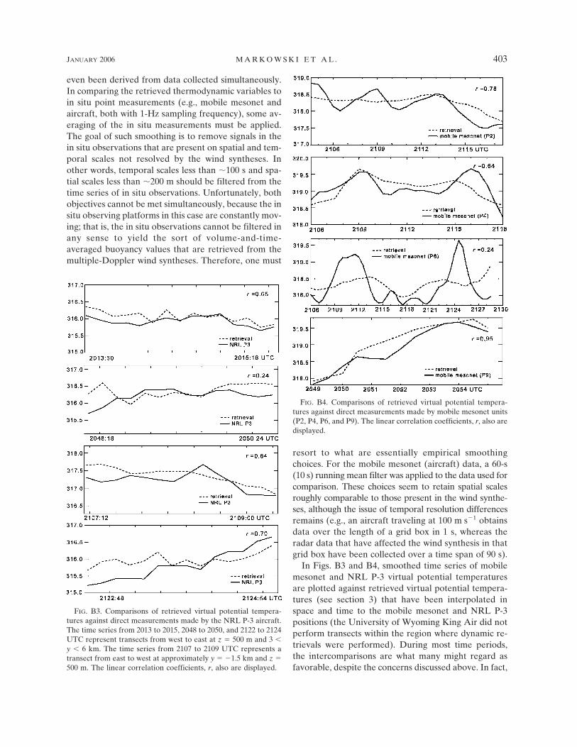
even been derived from data collected simultaneously.In comparing the retrieved thermodynamic variables toin situ point measurements (e.g., mobile mesonet andaircraft, both with 1-Hz sampling frequency), some av-eraging of the in situ measurements must be applied.The goal of such smoothing is to remove signals in thein situ observations that are present on spatial and tem-poral scales not resolved by the wind syntheses. Inother words, temporal scales less than �100 s and spa-tial scales less than �200 m should be filtered from thetime series of in situ observations. Unfortunately, bothobjectives cannot be met simultaneously, because the insitu observing platforms in this case are constantly mov-ing; that is, the in situ observations cannot be filtered inany sense to yield the sort of volume-and-time-averaged buoyancy values that are retrieved from themultiple-Doppler wind syntheses. Therefore, one must

resort to what are essentially empirical smoothingchoices. For the mobile mesonet (aircraft) data, a 60-s(10 s) running mean filter was applied to the data used forcomparison. These choices seem to retain spatial scalesroughly comparable to those present in the wind synthe-ses, although the issue of temporal resolution differencesremains (e.g., an aircraft traveling at 100 m s�1 obtainsdata over the length of a grid box in 1 s, whereas theradar data that have affected the wind synthesis in thatgrid box have been collected over a time span of 90 s).

In Figs. B3 and B4, smoothed time series of mobilemesonet and NRL P-3 virtual potential temperaturesare plotted against retrieved virtual potential tempera-tures (see section 3) that have been interpolated inspace and time to the mobile mesonet and NRL P-3positions (the University of Wyoming King Air did notperform transects within the region where dynamic re-trievals were performed). During most time periods,the intercomparisons are what many might regard asfavorable, despite the concerns discussed above. In fact,

FIG. B3. Comparisons of retrieved virtual potential tempera-tures against direct measurements made by the NRL P-3 aircraft.The time series from 2013 to 2015, 2048 to 2050, and 2122 to 2124UTC represent transects from west to east at z � 500 m and 3 �y � 6 km. The time series from 2107 to 2109 UTC represents atransect from east to west at approximately y � �1.5 km and z �500 m. The linear correlation coefficients, r, also are displayed.

FIG. B4. Comparisons of retrieved virtual potential tempera-tures against direct measurements made by mobile mesonet units(P2, P4, P6, and P9). The linear correlation coefficients, r, also aredisplayed.


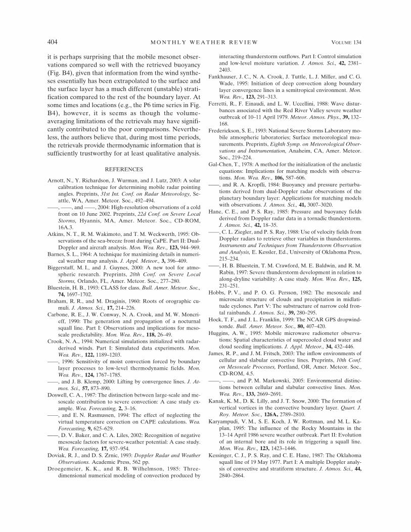
it is perhaps surprising that the mobile mesonet obser-vations compared so well with the retrieved buoyancy(Fig. B4), given that information from the wind synthe-ses essentially has been extrapolated to the surface andthe surface layer has a much different (unstable) strati-fication compared to the rest of the boundary layer. Atsome times and locations (e.g., the P6 time series in Fig.B4), however, it is seems as though the volume-averaging limitations of the retrievals may have signifi-cantly contributed to the poor comparisons. Neverthe-less, the authors believe that, during most time periods,the retrievals provide thermodynamic information that issufficiently trustworthy for at least qualitative analysis.

REFERENCES

Arnott, N., Y. Richardson, J. Wurman, and J. Lutz, 2003: A solarcalibration technique for determining mobile radar pointingangles. Preprints, 31st Int. Conf. on Radar Meteorology, Se-attle, WA, Amer. Meteor. Soc., 492–494.

——, ——, and ——, 2004: High-resolution observations of a coldfront on 10 June 2002. Preprints, 22d Conf. on Severe LocalStorms, Hyannis, MA, Amer. Meteor. Soc., CD-ROM,16A.3.

Atkins, N. T., R. M. Wakimoto, and T. M. Weckwerth, 1995: Ob-servations of the sea-breeze front during CaPE. Part II: Dual-Doppler and aircraft analysis. Mon. Wea. Rev., 123, 944–969.

Barnes, S. L., 1964: A technique for maximizing details in numeri-cal weather map analysis. J. Appl. Meteor., 3, 396–409.

Biggerstaff, M. I., and J. Guynes, 2000: A new tool for atmo-spheric research. Preprints, 20th Conf. on Severe LocalStorms, Orlando, FL, Amer. Meteor. Soc., 277–280.

Bluestein, H. B., 1993: CLASS for class. Bull. Amer. Meteor. Soc.,74, 1697–1702.

Braham, R. R., and M. Draginis, 1960: Roots of orographic cu-muli. J. Atmos. Sci., 17, 214–226.

Carbone, R. E., J. W. Conway, N. A. Crook, and M. W. Moncri-eff, 1990: The generation and propagation of a nocturnalsquall line. Part I: Observations and implications for meso-scale predictability. Mon. Wea. Rev., 118, 26–49.

Crook, N. A., 1994: Numerical simulations initialized with radar-derived winds. Part I: Simulated data experiments. Mon.Wea. Rev., 122, 1189–1203.

——, 1996: Sensitivity of moist convection forced by boundarylayer processes to low-level thermodynamic fields. Mon.Wea. Rev., 124, 1767–1785.

——, and J. B. Klemp, 2000: Lifting by convergence lines. J. At-mos. Sci., 57, 873–890.

Doswell, C. A., 1987: The distinction between large-scale and me-soscale contribution to severe convection: A case study ex-ample. Wea. Forecasting, 2, 3–16.

——, and E. N. Rasmussen, 1994: The effect of neglecting thevirtual temperature correction on CAPE calculations. Wea.Forecasting, 9, 625–629.

——, D. V. Baker, and C. A. Liles, 2002: Recognition of negativemesoscale factors for severe-weather potential: A case study.Wea. Forecasting, 17, 937–954.

Doviak, R. J., and D. S. Zrnic, 1993: Doppler Radar and WeatherObservations. Academic Press, 562 pp.

Droegemeier, K. K., and R. B. Wilhelmson, 1985: Three-dimensional numerical modeling of convection produced by

interacting thunderstorm outflows. Part I: Control simulationand low-level moisture variation. J. Atmos. Sci., 42, 2381–2403.

Fankhauser, J. C., N. A. Crook, J. Tuttle, L. J. Miller, and C. G.Wade, 1995: Initiation of deep convection along boundarylayer convergence lines in a semitropical environment. Mon.Wea. Rev., 123, 291–313.

Ferretti, R., F. Einaudi, and L. W. Uccellini, 1988: Wave distur-bances associated with the Red River Valley severe weatheroutbreak of 10–11 April 1979. Meteor. Atmos. Phys., 39, 132–168.

Frederickson, S. E., 1993: National Severe Storms Laboratory mo-bile atmospheric laboratories; Surface meteorological mea-surements. Preprints, Eighth Symp. on Meteorological Obser-vations and Instrumentation, Anaheim, CA, Amer. Meteor.Soc., 219–224.

Gal-Chen, T., 1978: A method for the initialization of the anelasticequations: Implications for matching models with observa-tions. Mon. Wea. Rev., 106, 587–606.

——, and R. A. Kropfli, 1984: Buoyancy and pressure perturba-tions derived from dual-Doppler radar observations of theplanetary boundary layer: Applications for matching modelswith observations. J. Atmos. Sci., 41, 3007–3020.

Hane, C. E., and P. S. Ray, 1985: Pressure and buoyancy fieldsderived from Doppler radar data in a tornadic thunderstorm.J. Atmos. Sci., 42, 18–35.

——, C. L. Ziegler, and P. S. Ray, 1988: Use of velocity fields fromDoppler radars to retrieve other variables in thunderstorms.Instruments and Techniques from Thunderstorm Observationand Analysis, E. Kessler, Ed., University of Oklahoma Press,215–234.

——, H. B. Bluestein, T. M. Crawford, M. E. Baldwin, and R. M.Rabin, 1997: Severe thunderstorm development in relation toalong-dryline variability: A case study. Mon. Wea. Rev., 125,231–251.

Hobbs, P. V., and P. O. G. Persson, 1982: The mesoscale andmicroscale structure of clouds and precipitation in midlati-tude cyclones. Part V: The substructure of narrow cold fron-tal rainbands. J. Atmos. Sci., 39, 280–295.

Hock, T. F., and J. L. Franklin, 1999: The NCAR GPS dropwind-sonde. Bull. Amer. Meteor. Soc., 80, 407–420.

Huggins, A. W., 1995: Mobile microwave radiometer observa-tions: Spatial characteristics of supercooled cloud water andcloud seeding implications. J. Appl. Meteor., 34, 432–446.

James, R. P., and J. M. Fritsch, 2003: The inflow environments ofcellular and slabular convective lines. Preprints, 10th Conf.on Mesoscale Processes, Portland, OR, Amer. Meteor. Soc.,CD-ROM, 4.5.

——, ——, and P. M. Markowski, 2005: Environmental distinc-tions between cellular and slabular convective lines. Mon.Wea. Rev., 133, 2669–2691.

Kanak, K. M., D. K. Lilly, and J. T. Snow, 2000: The formation ofvertical vortices in the convective boundary layer. Quart. J.Roy. Meteor. Soc., 126A, 2789–2810.

Karyampudi, V. M., S. E. Koch, J. W. Rottman, and M. L. Ka-plan, 1995: The influence of the Rocky Mountains in the13–14 April 1986 severe weather outbreak. Part II: Evolutionof an internal bore and its role in triggering a squall line.Mon. Wea. Rev., 123, 1423–1446.

Kessinger, C. J., P. S. Ray, and C. E. Hane, 1987: The Oklahomasquall line of 19 May 1977. Part I: A multiple Doppler analy-sis of convective and stratiform structure. J. Atmos. Sci., 44,2840–2864.


Kingsmill, D. E., 1995: Convection initiation associated with a sea-breeze front, a gust front, and their collision. Mon. Wea. Rev.,123, 2913–2933.

Koch, S. E., 1984: The role of an apparent mesoscale frontoge-netical circulation in squall line initiation. Mon. Wea. Rev.,112, 2090–2111.

——, and W. L. Clark, 1999: A nonclassical cold front observedduring COPS-91: Frontal structure and the process of severestorm initiation. J. Atmos. Sci., 56, 2862–2890.

——, M. DesJardins, and P. J. Kocin, 1983: An interactive Barnesobjective map analysis scheme for use with satellite and con-ventional data. J. Climate Appl. Meteor., 22, 1487–1503.

——, A. Aksakal, and J. T. McQueen, 1997: The influence ofmesoscale humidity and evapotranspiration fields on a modelforecast of a cold frontal squall line. Mon. Wea. Rev., 125,58–83.

Lee, B. D., and C. A. Finley, 2000: Simulating deep convectioninitiation by misocyclones. Preprints, 20th Conf. on SevereLocal Storms, Orlando, FL, Amer. Meteor. Soc., 70–73.

Lhermitte, R. M., and M. Gilet, 1975: Dual-Doppler observationand study of sea breeze convective storm development. J.Appl. Meteor., 14, 1346–1361.

Markowski, P., and C. Hannon, 2006: Multiple-Doppler radar ob-servations of the evolution of vorticity extrema in a convec-tive boundary layer. Mon. Wea. Rev., 134, 355–374.

Marquis, J., Y. P. Richardson, and J. Wurman, 2004: Observationsof misocyclones along boundaries during IHOP. Preprints,22d Conf. on Severe Local Storms, Hyannis, MA, Amer. Me-teor. Soc., CD-ROM, 16A.5.

Matejka, T., 2002: Estimating the most steady frame of referencefrom Doppler radar data. J. Atmos. Oceanic Technol., 19,1035–1048.

Matthews, D. A., 1981: Observations of a cloud arc triggered bythunderstorm outflow. Mon. Wea. Rev., 109, 2140–2157.

Ogura, Y., and Y.-L. Chen, 1977: A life history of an intensemesoscale convective storm in Oklahoma. J. Atmos. Sci., 34,1458–1476.

Orville, H. D., 1964: On mountain upslope winds. J. Atmos. Sci.,21, 622–633.

Parsons, D. B., C. G. Mohr, and T. Gal-Chen, 1987: A severefrontal rainband. Part III: Derived thermodynamic structure.J. Atmos. Sci., 44, 1613–1631.

Purdom, J. F. W., 1976: Some uses of high-resolution GOES im-agery in the mesoscale forecasting of convection and its be-havior. Mon. Wea. Rev., 104, 1474–1483.

Rasmussen, E. N., R. Davies-Jones, and R. L. Holle, 2003: Ter-restrial photogrammetry of weather images acquired in un-controlled circumstances. J. Atmos. Oceanic Technol., 20,1790–1803.

Ray, P. S., and K. L. Sangren, 1983: Multiple-Doppler radar net-work design. J. Climate Appl. Meteor., 22, 1444–1454.

Raymond, D., and M. Wilkening, 1980: Mountain-induced con-vection under fair weather conditions. J. Atmos. Sci., 37,2693–2706.

Rhea, J. O., 1966: A study of thunderstorm formation along drylines. J. Appl. Meteor., 5, 58–63.

Richardson, Y. P., J. Marquis, E. Rasmussen, J. Wurman, and N.Arnott, 2004: Analysis of convection initiation along a drylineon 19 June 2002. Preprints, 22d Conf. on Severe Local Storms,Hyannis, MA, Amer. Meteor. Soc., CD-ROM, 16A.4.

Rotunno, R., J. B. Klemp, and M. L. Weisman, 1988: A theory forstrong, long-lived squall lines. J. Atmos. Sci., 45, 463–485.

Roux, F., 1985: Retrieval of thermodynamic fields from multiple-

Doppler radar data using the equations of motion and thethermodynamic equation. Mon. Wea. Rev., 113, 2142–2157.

Schaefer, J. T., 1986: The dryline. Mesoscale Meteorology andForecasting, P. S. Ray, Ed., Amer. Meteor. Soc., 549–572.

Segal, M., and R. W. Arritt, 1992: Nonclassical mesoscale circu-lations caused by surface sensible heat-flux gradients. Bull.Amer. Meteor. Soc., 73, 1593–1604.

——, J. F. W. Purdom, J. L. Song, R. A. Pielke, and Y. Mahrer,1986: Evaluation of cloud shading effects on the generationand modification of mesoscale circulations. Mon. Wea. Rev.,114, 1201–1212.

Shapiro, A., and K. M. Kanak, 2002: Vortex formation in ellip-soidal thermal bubbles. J. Atmos. Sci., 59, 2253–2269.

Stonitsch, J., and P. Markowski, 2004: Evolution of boundarylayer wind and moisture fields along a front during IHOP.Preprints, 22d Conf. on Severe Local Storms, Hyannis, MA,Amer. Meteor. Soc., CD-ROM, 16A.7.

Straka, J. M., E. N. Rasmussen, and S. E. Fredrickson, 1996: Amobile mesonet for finescale meteorological observations. J.Atmos. Oceanic Technol., 13, 921–936.

Trapp, R. J., and C. A. Doswell, 2000: Radar data objective analy-sis. J. Atmos. Oceanic Technol., 17, 105–120.

Wakimoto, R. M., and N. T. Atkins, 1994: Observation of the sea-breeze front during CAPE. Part I: Single Doppler, satellite,and cloud photogrammetry analysis. Mon. Wea. Rev., 122,1092–1113.

Weckwerth, T. M., J. W. Wilson, and R. M. Wakimoto, 1996:Thermodynamic variability within the convective boundarylayer due to horizontal convective rolls. Mon. Wea. Rev., 124,769–784.

——, ——, ——, and N. A. Crook, 1997: Horizontal convectiverolls: Determining the environmental conditions supportingtheir existence and characteristics. Mon. Wea. Rev., 125, 505–526.

——, and Coauthors, 2004: An overview of the International H2OProject (IHOP) and some preliminary highlights. Bull. Amer.Meteor. Soc., 85, 253–277.

Weisman, M. L., 1992: The role of convectively generated rear-inflow jets in the evolution of long-lived mesoconvective sys-tems. J. Atmos. Sci., 49, 1826–1847.

Wilson, J. W., and W. E. Schreiber, 1986: Initiation of convectivestorms at radar-observed boundary-layer convergence lines.Mon. Wea. Rev., 114, 2516–2536.

——, G. B. Foote, N. A. Crook, J. C. Fankhauser, C. G. Wade,J. D. Tuttle, and C. K. Mueller, 1992: The role of boundary-layer convergence zones and horizontal rolls in the initiationof thunderstorms: A case study. Mon. Wea. Rev., 120, 1785–1815.

——, T. M. Weckwerth, J. Vivekanandan, R. M. Wakimoto, andR. W. Russell, 1994: Boundary layer clear-air radar echoes:Origin of echoes and accuracy of derived winds. J. Atmos.Oceanic Technol., 11, 1184–1206.

Wurman, J., J. Straka, E. Rasmussen, M. Randall, and A. Zahrai,1997: Design and deployment of a portable, pencil-beam,pulsed, 3-cm Doppler radar. J. Atmos. Oceanic Technol., 14,1502–1512.

Ziegler, C. L., and E. N. Rasmussen, 1998: The initiation of moistconvection at the dryline: Forecasting issues from a casestudy perspective. Wea. Forecasting, 13, 1106–1131.

——, T. J. Lee, and R. A. Pielke Sr., 1997: Convective initiation atthe dryline: A modeling study. Mon. Wea. Rev., 125, 1001–1026.


Observations of Convection Initiation “Failure” from the 12 June ...

Documents

Transcript of Observations of Convection Initiation “Failure” from the 12 June ...