observations mathematical models order-of-growth...

Algorithms, 4th Edition · Robert Sedgewick and Kevin Wayne · Copyright © 2002–2011 · February 8, 2012 5:59:31 AM

AlgorithmsF O U R T H E D I T I O N

R O B E R T S E D G E W I C K K E V I N W A Y N E

‣ observations‣ mathematical models‣ order-of-growth classifications‣ dependencies on inputs‣ memory

1.4 ANALYSIS OF ALGORITHMS

Cast of characters

2

Programmer needs to developa working solution.

Client wants to solveproblem efficiently.

Theoretician wants to understand.

Basic blocking and tacklingis sometimes necessary.[this lecture]

Student might playany or all of theseroles someday.

3

Running time

Analytic Engine

how many times do you have to turn the crank?

“ As soon as an Analytic Engine exists, it will necessarily guide the future course of the science. Whenever any result is sought by its aid, the question will arise—By what course of calculation can these results be arrived at by the machine in the shortest time? ” — Charles Babbage (1864)

Predict performance.

Compare algorithms.

Provide guarantees.

Understand theoretical basis.

Primary practical reason: avoid performance bugs.

Reasons to analyze algorithms

4

this course (COS 226)

theory of algorithms (COS 423)

client gets poor performance because programmerdid not understand performance characteristics

5

Some algorithmic successes

Discrete Fourier transform.

• Break down waveform of N samples into periodic components.

• Applications: DVD, JPEG, MRI, astrophysics, ….

• Brute force: N 2 steps.

• FFT algorithm: N log N steps, enables new technology.Friedrich Gauss

1805

8T

16T

32T

64T

time

1K 2K 4K 8Ksize

quadratic

linearithmic

linear

6

Some algorithmic successes

N-body simulation.

• Simulate gravitational interactions among N bodies.

• Brute force: N 2 steps.

• Barnes-Hut algorithm: N log N steps, enables new research. Andrew AppelPU '81

8T

16T

32T

64T

time

1K 2K 4K 8Ksize

quadratic

linearithmic

linear

Q. Will my program be able to solve a large practical input?

Key insight. [Knuth 1970s] Use scientific method to understand performance.

The challenge

7

Why is my program so slow ? Why does it run out of memory ?

8

Scientific method applied to analysis of algorithms

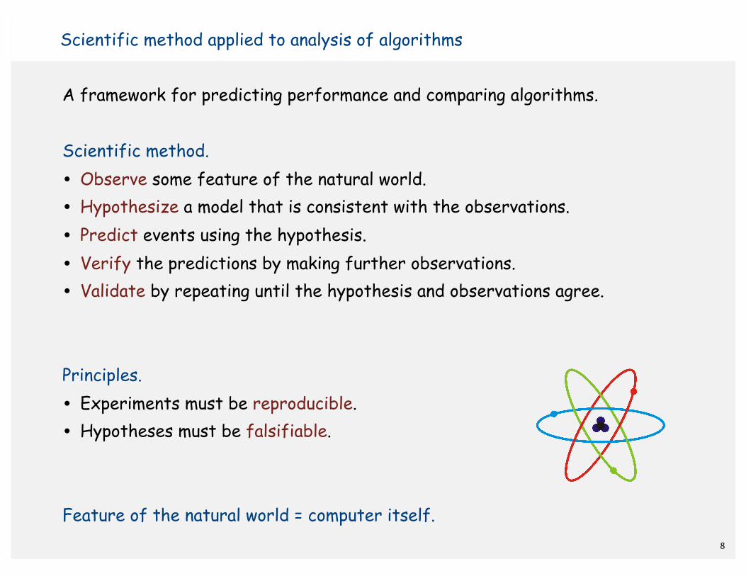
A framework for predicting performance and comparing algorithms.

Scientific method.

• Observe some feature of the natural world.

• Hypothesize a model that is consistent with the observations.

• Predict events using the hypothesis.

• Verify the predictions by making further observations.

• Validate by repeating until the hypothesis and observations agree.

Principles.

• Experiments must be reproducible.

• Hypotheses must be falsifiable.

Feature of the natural world = computer itself.

9


10

Example: 3-sum

3-sum. Given N distinct integers, how many triples sum to exactly zero?

Context. Deeply related to problems in computational geometry.

% more 8ints.txt830 -40 -20 -10 40 0 10 5

% java ThreeSum 8ints.txt4

a[i] a[j] a[k] sum

30 -40 10 0

30 -20 -10 0

-40 40 0 0

-10 0 10 0

1

2

3

4

public class ThreeSum{ public static int count(int[] a) { int N = a.length; int count = 0; for (int i = 0; i < N; i++) for (int j = i+1; j < N; j++) for (int k = j+1; k < N; k++) if (a[i] + a[j] + a[k] == 0) count++; return count; }

public static void main(String[] args) { int[] a = In.readInts(args[0]); StdOut.println(count(a)); }}

11

3-sum: brute-force algorithm

check each triple

for simplicity, ignore integer overflow

Q. How to time a program?A. Manual.

12

Measuring the running time

% java ThreeSum 1Kints.txt

70



528

4039

tick tick tick

Observing the running time of a program

tick tick tick tick tick tick tick ticktick tick tick tick tick tick tick ticktick tick tick tick tick tick tick tick

tick tick tick tick tick tick tick ticktick tick tick tick tick tick tick ticktick tick tick tick tick tick tick ticktick tick tick tick tick tick tick ticktick tick tick tick tick tick tick ticktick tick tick tick tick tick tick ticktick tick tick tick tick tick tick ticktick tick tick tick tick tick tick ticktick tick tick tick tick tick tick ticktick tick tick tick tick tick tick ticktick tick tick tick tick tick tick ticktick tick tick tick tick tick tick ticktick tick tick tick tick tick tick ticktick tick tick tick tick tick tick ticktick tick tick tick tick tick tick ticktick tick tick tick tick tick tick ticktick tick tick tick tick tick tick ticktick tick tick tick tick tick tick ticktick tick tick tick tick tick tick ticktick tick tick tick tick tick tick ticktick tick tick tick tick tick tick ticktick tick tick tick tick tick tick ticktick tick tick tick tick tick tick ticktick tick tick tick tick tick tick tick

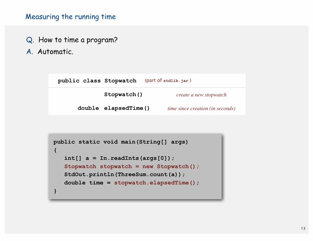
Q. How to time a program?A. Automatic.

13

Measuring the running time

client code

public static void main(String[] args){ int[] a = In.readInts(args[0]); Stopwatch stopwatch = new Stopwatch(); StdOut.println(ThreeSum.count(a)); double time = stopwatch.elapsedTime();}

public class Stopwatch public class Stopwatch

Stopwatch()Stopwatch() create a new stopwatch

double elapsedTime()elapsedTime() time since creation (in seconds)

(part of stdlib.jar )

Run the program for various input sizes and measure running time.

14

Empirical analysis

N time (seconds) †

250 0.0

500 0.0

1,000 0.1

2,000 0.8

4,000 6.4

8,000 51.1

16,000 ?

Standard plot. Plot running time T (N) vs. input size N.

15

Data analysis

1K

.1

.2

.4

.8

1.6

3.2

6.4

12.8

25.6

51.2

Analysis of experimental data (the running time of ThreeSum)

log-log plotstandard plot

lgNproblem size N2K 4K 8K

lg(T

(N))

runn

ing

tim

e T

(N)

1K

10

20

30

40

50

2K 4K 8K

straight lineof slope 3

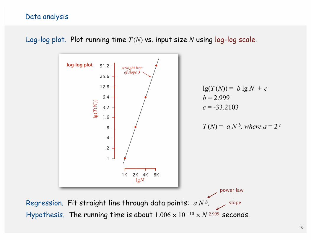
Log-log plot. Plot running time T (N) vs. input size N using log-log scale.

Regression. Fit straight line through data points: a N b.Hypothesis. The running time is about 1.006 × 10 –10 × N 2.999 seconds.

16

Data analysis

slope

power law

1K

.1

.2

.4

.8

1.6

3.2

6.4

12.8

25.6

51.2

Analysis of experimental data (the running time of ThreeSum)

log-log plotstandard plot

lgNproblem size N2K 4K 8K

lg(T

(N))

runn

ing

tim

e T

(N)

1K

10

20

30

40

50

2K 4K 8K

straight lineof slope 3

lg(T (N)) = b lg N + cb = 2.999c = -33.2103

T (N) = a N b, where a = 2 c

17

Prediction and validation

Hypothesis. The running time is about 1.006 × 10 –10 × N 2.999 seconds.

Predictions.

• 51.0 seconds for N = 8,000.

• 408.1 seconds for N = 16,000.

Observations.

validates hypothesis!


8,000 51.1

8,000 51.0

8,000 51.1

16,000 410.8

"order of growth" of runningtime is about N3 [stay tuned]

Doubling hypothesis. Quick way to estimate b in a power-law relationship.

Run program, doubling the size of the input.

Hypothesis. Running time is about a N b with b = lg ratio. Caveat. Cannot identify logarithmic factors with doubling hypothesis.

18

Doubling hypothesis

N time (seconds) † ratio lg ratio

250 0.0 –

500 0.0 4.8 2.3

1,000 0.1 6.9 2.8

2,000 0.8 7.7 2.9

4,000 6.4 8.0 3.0

8,000 51.1 8.0 3.0

seems to converge to a constant b ≈ 3

19

Doubling hypothesis

Doubling hypothesis. Quick way to estimate b in a power-law hypothesis.

Q. How to estimate a (assuming we know b) ?A. Run the program (for a sufficient large value of N) and solve for a.

Hypothesis. Running time is about 0.998 × 10 –10 × N 3 seconds.


8,000 51.1

8,000 51.0

8,000 51.1

51.1 = a × 80003

⇒ a = 0.998 × 10 –10

almost identical hypothesisto one obtained via linear regression

20

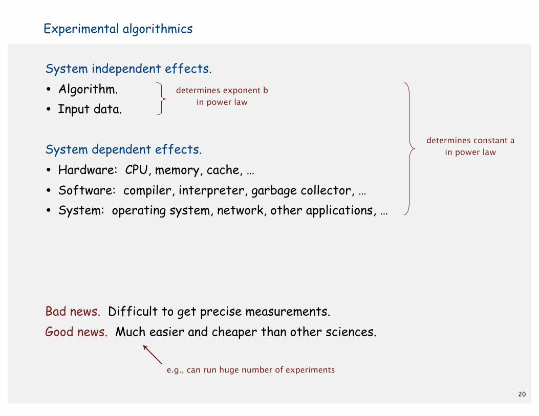
Experimental algorithmics

System independent effects.

• Algorithm.

• Input data.

System dependent effects.

• Hardware: CPU, memory, cache, …

• Software: compiler, interpreter, garbage collector, …

• System: operating system, network, other applications, …

Bad news. Difficult to get precise measurements.Good news. Much easier and cheaper than other sciences.

e.g., can run huge number of experiments

determines exponent bin power law

determines constant ain power law

21

War story (from COS 126)

Q. How long does this program take as a function of N ?

String s = StdIn.readString(); int N = s.length(); ... for (int i = 0; i < N; i++) for (int j = 0; j < N; j++) distance[i][j] = ... ...

N time

1,000 0.11

2,000 0.35

4,000 1.6

8,000 6.5

N time

250 0.5

500 1.1

1,000 1.9

2,000 3.9

Jenny ~ c1 N2 seconds Kenny ~ c2 N seconds

22


23

Mathematical models for running time

Total running time: sum of cost × frequency for all operations.

• Need to analyze program to determine set of operations.

• Cost depends on machine, compiler.

• Frequency depends on algorithm, input data.

In principle, accurate mathematical models are available.

Donald Knuth1974 Turing Award

Cost of basic operations

operation example nanoseconds †

integer add a + b 2.1

integer multiply a * b 2.4

integer divide a / b 5.4

floating-point add a + b 4.6

floating-point multiply a * b 4.2

floating-point divide a / b 13.5

sine Math.sin(theta) 91.3

arctangent Math.atan2(y, x) 129.0

... ... ...

24

† Running OS X on Macbook Pro 2.2GHz with 2GB RAM

Novice mistake. Abusive string concatenation.

Cost of basic operations

25

operation example nanoseconds †

variable declaration int a c1

assignment statement a = b c2

integer compare a < b c3

array element access a[i] c4

array length a.length c5

1D array allocation new int[N] c6 N

2D array allocation new int[N][N] c7 N 2

string length s.length() c8

substring extraction s.substring(N/2, N) c9

string concatenation s + t c10 N

Q. How many instructions as a function of input size N ?

26

Example: 1-sum

int count = 0;for (int i = 0; i < N; i++) if (a[i] == 0) count++;

operation frequency

variable declaration 2

assignment statement 2

less than compare N + 1

equal to compare N

array access N

increment N to 2 N

27

Example: 2-sum

Q. How many instructions as a function of input size N ?

operation frequency

variable declaration N + 2

assignment statement N + 2

less than compare ½ (N + 1) (N + 2)

equal to compare ½ N (N − 1)

array access N (N − 1)

increment ½ N (N − 1) to N (N − 1)

tedious to count exactly

0 + 1 + 2 + . . . + (N � 1) =12

N (N � 1)

=�

N

2

⇥

int count = 0;for (int i = 0; i < N; i++) for (int j = i+1; j < N; j++) if (a[i] + a[j] == 0) count++;

28

Simplifying the calculations

“ It is convenient to have a measure of the amount of work involved in a computing process, even though it be a very crude one. We may count up the number of times that various elementary operations are applied in the whole process and then given them various weights. We might, for instance, count the number of additions, subtractions, multiplications, divisions, recording of numbers, and extractions of figures from tables. In the case of computing with matrices most of the work consists of multiplications and writing down numbers, and we shall therefore only attempt to count the number of multiplications and recordings. ” — Alan Turing

ROUNDING-OFF ERRORS IN MATRIX PROCESSESBy A. M. TURING

{National Physical Laboratory, Teddington, Middlesex)[Received 4 November 1947]

SUMMARYA number of methods of solving sets of linear equations and inverting matrices

are discussed. The theory of the rounding-off errors involved is investigated forsome of the methods. In all cases examined, including the well-known 'Gausselimination process', it is found that the errors are normally quite moderate: noexponential build-up need occur.

Included amongst the methods considered is a generalization of Choleski's methodwhich appears to have advantages over other known methods both as regardsaccuracy and convenience. This method may also be regarded as a rearrangementof the elimination process.THIS paper contains descriptions of a number of methods for solving setsof linear simultaneous equations and for inverting matrices, but its mainconcern is with the theoretical limits of accuracy that may be obtained inthe application of these methods, due to rounding-off errors.

The best known method for the solution of linear equations is Gauss'selimination method. This is the method almost universally taught inschools. It has, unfortunately, recently come into disrepute on the groundthat rounding off will give rise to very large errors. It has, for instance,been argued by HoteUing (ref. 5) that in solving a set of n equations weshould keep nlog104 extra or 'guarding' figures. Actually, althoughexamples can be constructed where as many as «log102 extra figureswould be required, these are exceptional. In the present paper themagnitude of the error is described in terms of quantities not consideredin HoteUing's analysis; from the inequalities proved here it can imme-diately be seen that in all normal cases the Hotelling estimate is far toopessimistic.

The belief that the elimination method and other 'direct' methods ofsolution lead to large errors has been responsible for a recent search forother methods which would be free from this weakness. These weremainly methods of successive approximation and considerably morelaborious than the direct ones. There now appears to be no real advantagein the indirect methods, except in connexion with matrices having specialproperties, for example, where the vast majority of the coefficients arevery small, but there is at least one large one in each row.

The writer was prompted to cany out this research largely by thepractical work of L. Fox in applying the elimination method (ref. 2). Fox

at Princeton University Library on Septem

ber 20, 2011qjm

am.oxfordjournals.org

Dow

nloaded from

operation frequency

variable declaration N + 2

assignment statement N + 2

less than compare ½ (N + 1) (N + 2)

equal to compare ½ N (N − 1)

array access N (N − 1)

increment ½ N (N − 1) to N (N − 1)

29

Simplification 1: cost model

Cost model. Use some basic operation as a proxy for running time.

cost model = array accesses

0 + 1 + 2 + . . . + (N � 1) =12

N (N � 1)

=�

N

2

⇥


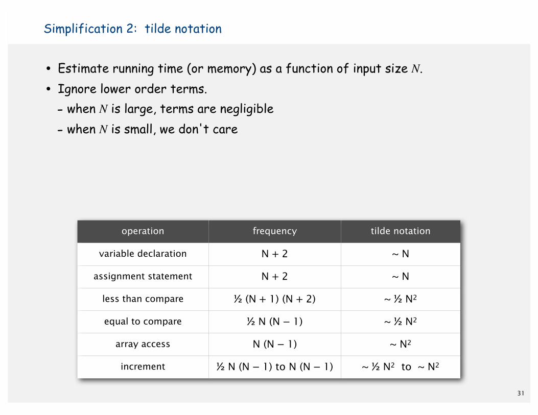
• Estimate running time (or memory) as a function of input size N.

• Ignore lower order terms.- when N is large, terms are negligible

- when N is small, we don't care

Ex 1. ⅙ N 3 + 20 N + 16 ~ ⅙ N 3

Ex 2. ⅙ N 3 + 100 N 4/3 + 56 ~ ⅙ N 3

Ex 3. ⅙ N 3 - ½ N 2 + ⅓ N ~ ⅙ N 3

30

Simplification 2: tilde notation

discard lower-order terms(e.g., N = 1000: 500 thousand vs. 166 million)

Technical definition. f(N) ~ g(N) means

€

limN→ ∞

f (N)g(N)

= 1

Leading-term approximation

N 3/6

N 3/6 ! N 2/2 + N /3

166,167,000

1,000

166,666,667

N

• Estimate running time (or memory) as a function of input size N.

• Ignore lower order terms.- when N is large, terms are negligible

- when N is small, we don't care

31

Simplification 2: tilde notation

operation frequency tilde notation

variable declaration N + 2 ~ N

assignment statement N + 2 ~ N

less than compare ½ (N + 1) (N + 2) ~ ½ N2

equal to compare ½ N (N − 1) ~ ½ N2

array access N (N − 1) ~ N2

increment ½ N (N − 1) to N (N − 1) ~ ½ N2 to ~ N2

Q. Approximately how many array accesses as a function of input size N ?

A. ~ N 2 array accesses.

Bottom line. Use cost model and tilde notation to simplify frequency counts.


32

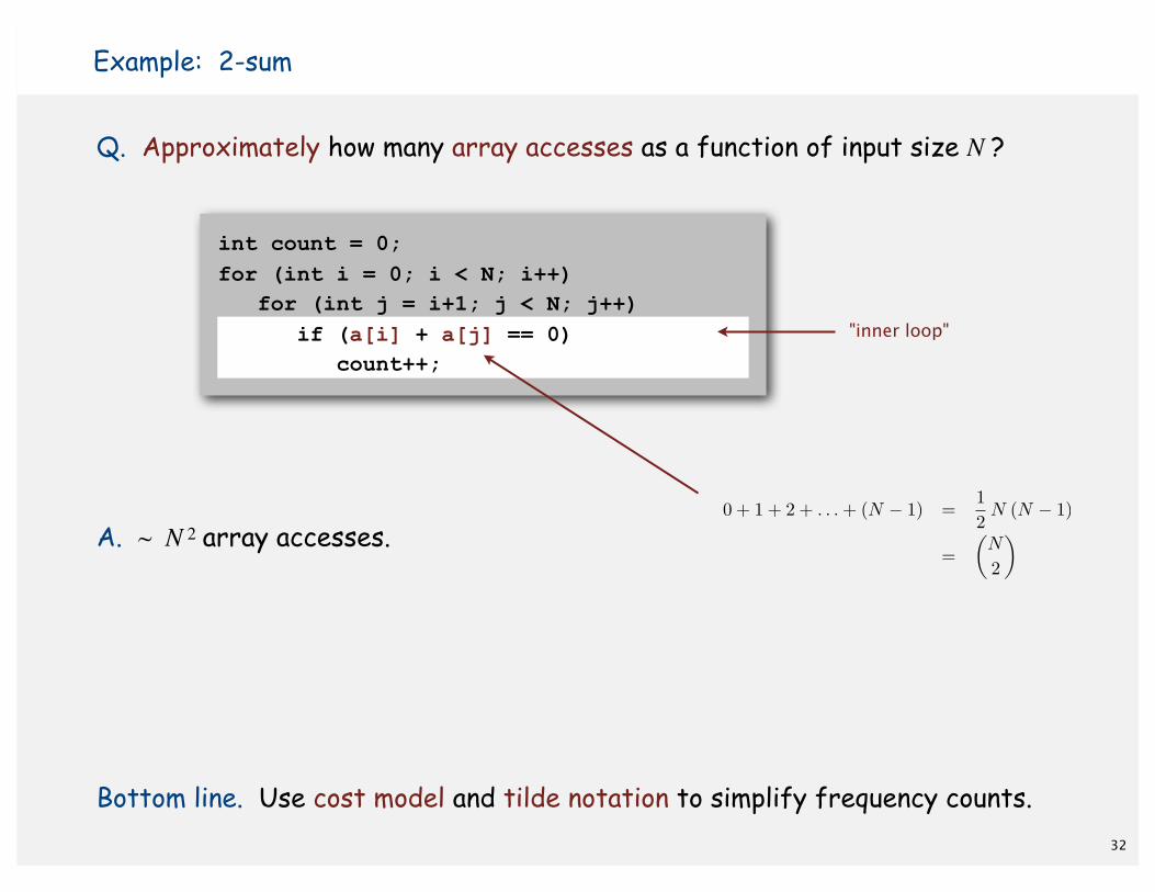
Example: 2-sum

"inner loop"

0 + 1 + 2 + . . . + (N � 1) =12

N (N � 1)

=�

N

2

⇥

Q. Approximately how many array accesses as a function of input size N ?

A. ~ ½ N 3 array accesses.

Bottom line. Use cost model and tilde notation to simplify frequency counts.

int count = 0;for (int i = 0; i < N; i++) for (int j = i+1; j < N; j++) for (int k = j+1; k < N; k++) if (a[i] + a[j] + a[k] == 0) count++;

33

Example: 3-sum

�N

3

⇥=

N(N � 1)(N � 2)3!

⇥ 16N3

"inner loop"

34

Estimating a discrete sum

Q. How to estimate a discrete sum?A1. Take COS 340.A2. Replace the sum with an integral, and use calculus!

Ex 1. 1 + 2 + … + N.

Ex 2. 1 + 1/2 + 1/3 + … + 1/N.

Ex 3. 3-sum triple loop.

N�

i=1

1i�

⇥ N

x=1

1x

dx = lnN

N�

i=1

i �⇥ N

x=1x dx � 1

2N2

N�

i=1

N�

j=i

N�

k=j

1 �⇥ N

x=1

⇥ N

y=x

⇥ N

z=ydz dy dx � 1

6N3

In principle, accurate mathematical models are available.

In practice,

• Formulas can be complicated.

• Advanced mathematics might be required.

• Exact models best left for experts.

Bottom line. We use approximate models in this course: T(N) ~ c N 3.

TN = c1 A + c2 B + c3 C + c4 D + c5 EA = array access B = integer add

C = integer compare

D = increment

E = variable assignment

Mathematical models for running time

35

frequencies (depend on algorithm, input)

costs (depend on machine, compiler)

36


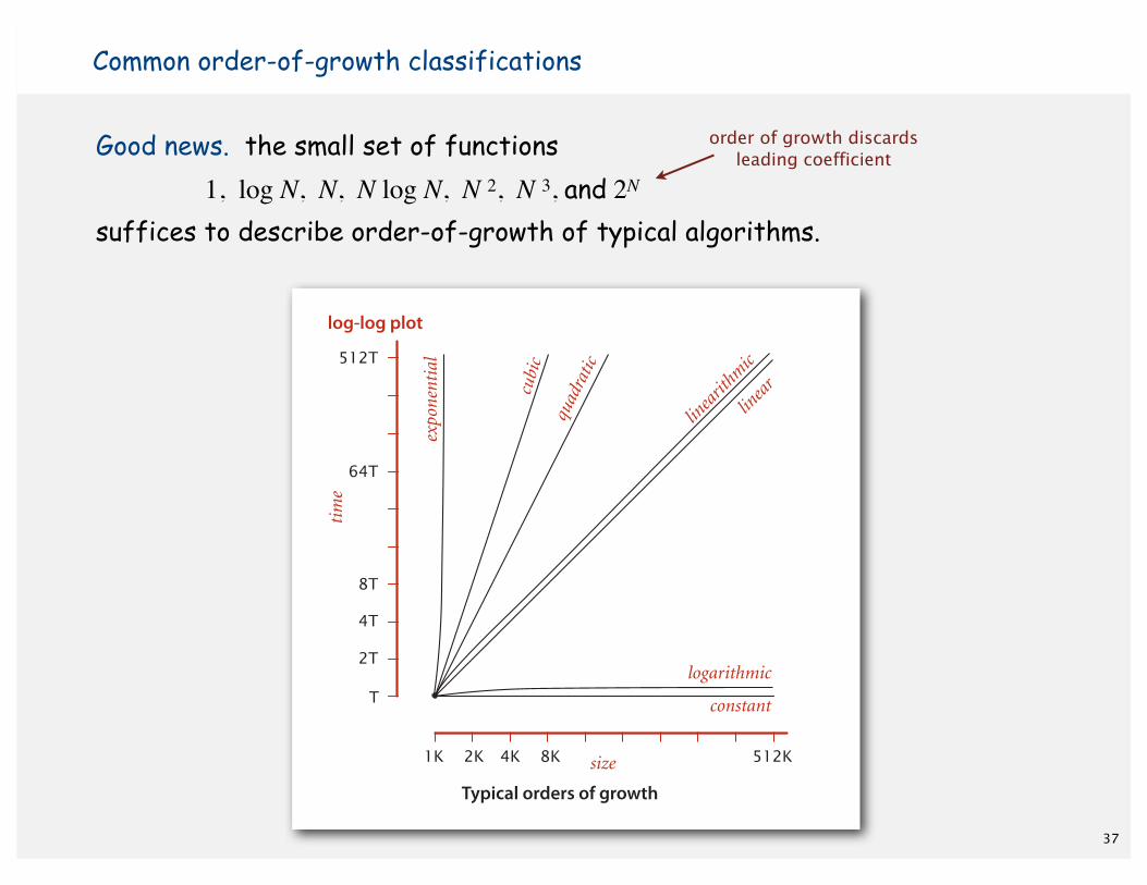
Good news. the small set of functions 1, log N, N, N log N, N 2, N 3, and 2N

suffices to describe order-of-growth of typical algorithms.

Common order-of-growth classifications

37

1K

T

2T

4T

8T

64T

512T

logarithmic

expo

nent

ial

constant

linea

rithmic

linea

r

quad

ratic

cubi

c

2K 4K 8K 512K

100T

200T

500T

logarithmic

exponential

constant

size

size

linea

rithmic

linea

r

100K 200K 500K

tim

eti

me

Typical orders of growth

log-log plot

standard plot

cubicquadratic

order of growth discardsleading coefficient

Common order-of-growth classifications

38

order of growth name typical code framework description example T(2N) / T(N)

1 constant a = b + c; statementadd two numbers

1

log N logarithmic while (N > 1){ N = N / 2; ... } divide in half binary search ~ 1

N linear for (int i = 0; i < N; i++){ ... } loop

find the maximum

2

N log N linearithmic [see mergesort lecture]divide

and conquermergesort ~ 2

N2 quadraticfor (int i = 0; i < N; i++)

for (int j = 0; j < N; j++) { ... }

double loopcheck all

pairs4

N3 cubic

for (int i = 0; i < N; i++) for (int j = 0; j < N; j++)

for (int k = 0; k < N; k++) { ... }

triple loopcheck all triples

8

2N exponential [see combinatorial search lecture]exhaustive

searchcheck all subsets

T(N)

Bottom line. Need linear or linearithmic alg to keep pace with Moore's law.

Practical implications of order-of-growth

39

growthrate

problem size solvable in minutesproblem size solvable in minutes

rate1970s 1980s 1990s 2000s

1 any any any any

log N any any any any

N millionstens ofmillions

hundreds ofmillions

billions

N log Nhundreds ofthousands

millions millionshundreds of

millions

N2 hundreds thousand thousandstens of

thousands

N3 hundred hundreds thousand thousands

2N 20 20s 20s 30

40

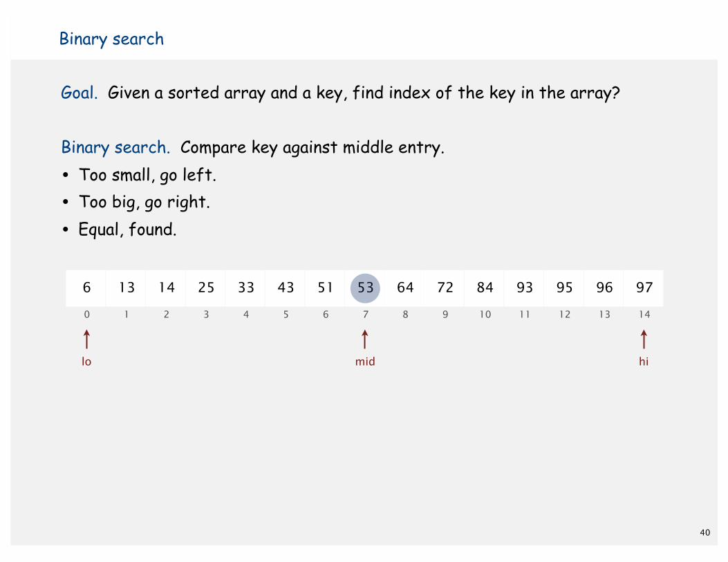
Binary search

Goal. Given a sorted array and a key, find index of the key in the array?

Binary search. Compare key against middle entry.

• Too small, go left.

• Too big, go right.

• Equal, found.

lo

6 13 14 25 33 43 51 53 64 72 84 93 95 96 97

0 1 2 3 4 5 6 7 8 9 10 11 12 13 14

himid

41

Binary search demo

42

Binary search: Java implementation

Trivial to implement?

• First binary search published in 1946; first bug-free one published in 1962.

• Java bug in Arrays.binarySearch() discovered in 2006.

Invariant. If key appears in the array a[], then a[lo] ≤ key ≤ a[hi].

public static int binarySearch(int[] a, int key) { int lo = 0, hi = a.length-1; while (lo <= hi) { int mid = lo + (hi - lo) / 2; if (key < a[mid]) hi = mid - 1; else if (key > a[mid]) lo = mid + 1; else return mid; } return -1; }

one "3-way compare"

43

Binary search: mathematical analysis

Proposition. Binary search uses at most 1 + lg N compares to search in asorted array of size N.

Def. T (N) ≡ # compares to binary search in a sorted subarray of size at most N.

Binary search recurrence. T (N) ≤ T (N / 2) + 1 for N > 1, with T (1) = 1.

Pf sketch. left or right half

T (N) ≤ T (N / 2) + 1

≤ T (N / 4) + 1 + 1

≤ T (N / 8) + 1 + 1 + 1

. . .

≤ T (N / N) + 1 + 1 + … + 1

= 1 + lg N

given

apply recurrence to first term

apply recurrence to first term

stop applying, T(1) = 1

possible to implement with one2-way compare (instead of 3-way)

Algorithm.

• Sort the N (distinct) numbers.

• For each pair of numbers a[i] and a[j],binary search for -(a[i] + a[j]).

Analysis. Order of growth is N 2 log N.

• Step 1: N 2 with insertion sort.

• Step 2: N 2 log N with binary search.

input 30 -40 -20 -10 40 0 10 5

sort -40 -20 -10 0 5 10 30 40

binary search(-40, -20) 60(-40, -10) 30(-40, 0) 40(-40, 5) 35(-40, 10) 30 ⋮ ⋮

(-40, 40) 0 ⋮ ⋮

(-10, 0) 10 ⋮ ⋮

(-20, 10) 10 ⋮ ⋮

( 10, 30) -40( 10, 40) -50( 30, 40) -70

An N2 log N algorithm for 3-sum

44

only count ifa[i] < a[j] < a[k]

to avoiddouble counting

Comparing programs

Hypothesis. The N 2 log N three-sum algorithm is significantly fasterin practice than the brute-force N 3 algorithm.

Guiding principle. Typically, better order of growth ⇒ faster in practice.45

N time (seconds)

1,000 0.14

2,000 0.18

4,000 0.34

8,000 0.96

16,000 3.67

32,000 14.88

64,000 59.16

N time (seconds)

1,000 0.1

2,000 0.8

4,000 6.4

8,000 51.1

ThreeSum.java

ThreeSumDeluxe.java

46


Best case. Lower bound on cost.

• Determined by “easiest” input.

• Provides a goal for all inputs.

Worst case. Upper bound on cost.

• Determined by “most difficult” input.

• Provides a guarantee for all inputs.

Average case. Expected cost for random input.

• Need a model for “random” input.

• Provides a way to predict performance.

Types of analyses

47

Ex 1. Array accesses for brute-force 3 sum. Best: ~ ½ N 3

Average: ~ ½ N 3

Worst: ~ ½ N 3

Ex 2. Compares for binary search.Best: ~ 1

Average: ~ lg N

Worst: ~ lg N

Common mistake. Interpreting big-Oh as an approximate model.

48

Commonly-used notations

notation provides example shorthand for used to

Tilde leading term ~ 10 N2

10 N2

10 N2 + 22 N log N10 N2 + 2 N + 37

provideapproximate

model

Big Thetaasymptoticgrowth rate

Θ(N2)½ N2

10 N2

5 N2 + 22 N log N + 3N

classifyalgorithms

Big Oh Θ(N2) and smaller O(N2)10 N2

100 N 22 N log N + 3 N

developupper bounds

Big Omega Θ(N2) and larger Ω(N2)

½ N2

N5

N3 + 22 N log N + 3 N

developlower bounds

49


50

Basics

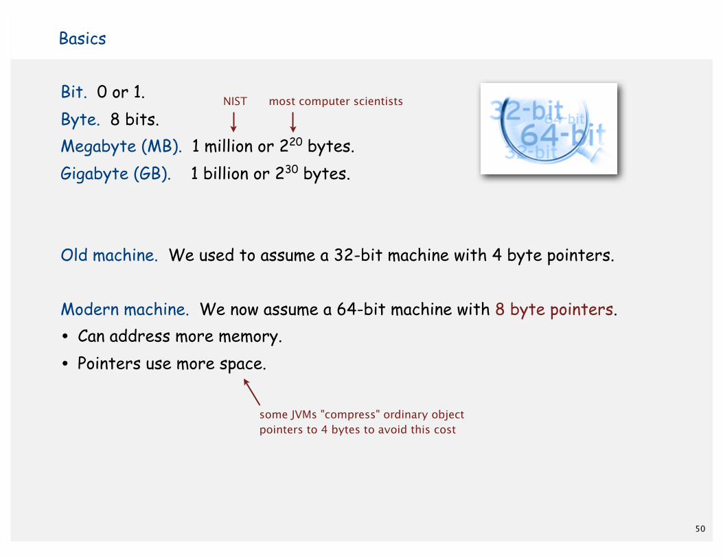
Bit. 0 or 1.Byte. 8 bits.Megabyte (MB). 1 million or 220 bytes.Gigabyte (GB). 1 billion or 230 bytes.

Old machine. We used to assume a 32-bit machine with 4 byte pointers.

Modern machine. We now assume a 64-bit machine with 8 byte pointers.

• Can address more memory.

• Pointers use more space.

some JVMs "compress" ordinary objectpointers to 4 bytes to avoid this cost

NIST most computer scientists

51

Typical memory usage for primitive types and arrays

Primitive types. Array overhead. 24 bytes.

type bytes

boolean 1

byte 1

char 2

int 4

float 4

long 8

double 8

for primitive types

type bytes

char[] 2N + 24

int[] 4N + 24

double[] 8N + 24

type bytes

char[][] ~ 2 M N

int[][] ~ 4 M N

double[][] ~ 8 M N

for one-dimensional arrays

for two-dimensional arrays

Object overhead. 16 bytes.Reference. 8 bytes.Padding. Each object uses a multiple of 8 bytes.

Ex 1. A Date object uses 32 bytes of memory.

public class Integer{ private int x;...}

Typical object memory requirements

objectoverhead

public class Node{ private Item item; private Node next;...}

public class Counter{ private String name; private int count;...}

24 bytesinteger wrapper object

counter object

node object (inner class)

32 bytes

intvalue

intvalue

Stringreference

public class Date{ private int day; private int month; private int year;...}

date object

x

objectoverhead

name

count

40 bytes

references

objectoverhead

extraoverhead

item

next

32 bytes

intvalues

objectoverhead

yearmonthday

padding

padding

padding

52

Typical memory usage for objects in Java

4 bytes (int)

4 bytes (int)

16 bytes (object overhead)

32 bytes

4 bytes (int)

4 bytes (padding)

Object overhead. 16 bytes.Reference. 8 bytes.Padding. Each object uses a multiple of 8 bytes.

Ex 2. A virgin String of length N uses ~ 2N bytes of memory.

A String and a substring

String genome = "CGCCTGGCGTCTGTAC";String codon = genome.substring(6, 3);

16

objectoverhead

charvalues

C GC CT GG CG TC TG TA C

016

objectoverhead

genome

63

objectoverhead

codon

hash

hash

...

value

public class String{ private char[] value; private int offset; private int count; private int hash;...} offset

count hash

objectoverhead

40 bytes

40 bytes

40 bytes

36 bytes

String object (Java library)

substring example

reference

intvalues

padding

padding

padding

padding

value

value

53

Typical memory usage for objects in Java

8 bytes (reference to array)

4 bytes (int)

4 bytes (int)

2N + 24 bytes (char[] array)

16 bytes (object overhead)

2N + 64 bytes

4 bytes (int)

4 bytes (padding)

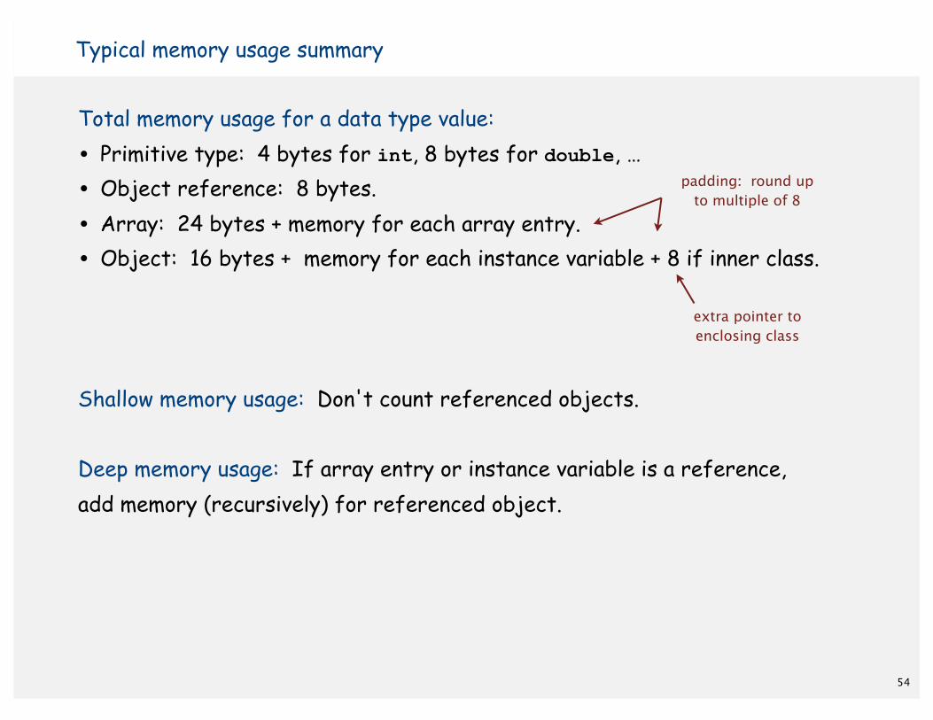
Total memory usage for a data type value:

• Primitive type: 4 bytes for int, 8 bytes for double, …

• Object reference: 8 bytes.

• Array: 24 bytes + memory for each array entry.

• Object: 16 bytes + memory for each instance variable + 8 if inner class.

Shallow memory usage: Don't count referenced objects.

Deep memory usage: If array entry or instance variable is a reference,add memory (recursively) for referenced object.

54

Typical memory usage summary

extra pointer toenclosing class

padding: round upto multiple of 8

55

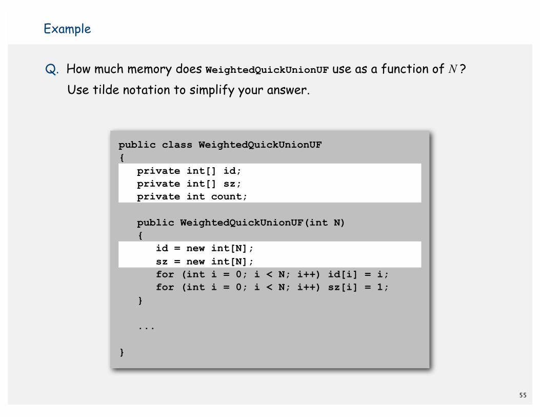
Example

Q. How much memory does WeightedQuickUnionUF use as a function of N ? Use tilde notation to simplify your answer.

public class WeightedQuickUnionUF{ private int[] id; private int[] sz; private int count; public WeightedQuickUnionUF(int N) { id = new int[N]; sz = new int[N]; for (int i = 0; i < N; i++) id[i] = i; for (int i = 0; i < N; i++) sz[i] = 1; }

...

}

Turning the crank: summary

Empirical analysis.

• Execute program to perform experiments.

• Assume power law and formulate a hypothesis for running time.

• Model enables us to make predictions.

Mathematical analysis.

• Analyze algorithm to count frequency of operations.

• Use tilde notation to simplify analysis.

• Model enables us to explain behavior.

Scientific method.

• Mathematical model is independent of a particular system;applies to machines not yet built.

• Empirical analysis is necessary to validate mathematical modelsand to make predictions.

56

observations mathematical models order-of-growth...

Documents

Transcript of observations mathematical models order-of-growth...