Observation of Solar Wind Charge Exchange Emission fromExospheric Material in and outside Earth’s Magnetosheath

May 14, 2008

S. L. Snowden,1,2 M. R. Collier,3 T. Cravens,4 K. D. Kuntz,5 S. T. Lepri,6 I. Robertson4

andL. Tomas7

ABSTRACT

A long XMM-Newton exposure is used to observe solar wind charge exchange (SWCX) emis-sion from exospheric material in and outside Earth’s magnetosheath. The light curve of the O VII

(0.5−0.62 keV) band is compared with a model for the expected emission, and while the emissionis faint and the light curve has considerable scatter, the correlation is significant to better than99.9%. This result demonstrates the validity of the geocoronal SWCX emission model for predict-ing a contribution to astrophysical observations to a scale factor of order unity (1.36). The resultsalso demonstrate the potential utility of using X-ray observations to study global phenomena ofthe magnetosheath which currently are only investigated using in situ measurements.

Subject headings: X-rays: general, X-rays: ISM, solar system: general, interplanetary medium, (Sun:)solar wind

1. Introduction

Diffuse X-ray emission from the solar sys-tem has been observed for several decades as anunidentified contamination component in observa-tions of the soft X-ray background. It was seen inthe Wisconsin sounding-rocket survey data as off-sets between overlapping parts of adjacent fields(McCammon et al. 1983; Burrows 1982), and inthe HEAO-1 A2 maps (Garmire et al. 1992) as

1Code 662, NASA/Goddard Space Flight Center,Greenbelt, MD 20771

2Steven.L.Snowden@nasa.gov3Code 673, NASA/Goddard Space Flight Center,

Greenbelt, MD 207714Department of Physics and Astronomy, University of

Kansas, Lawrence, Kansas5Henry A. Rowland Department of Physics and Astron-

omy, The Johns Hopkins University, 366 Bloomberg Cen-ter, 3400 N. Charles Street, Baltimore, MD 21218

6Department of Atmospheric, Oceanic, and Space Sci-ences, The University of Michigan, Ann Arbor, MI.

7European Space Astronomy Centre, European SpaceAgency, P.O. Box 78, Villanueva de la Caada, 28691Madrid

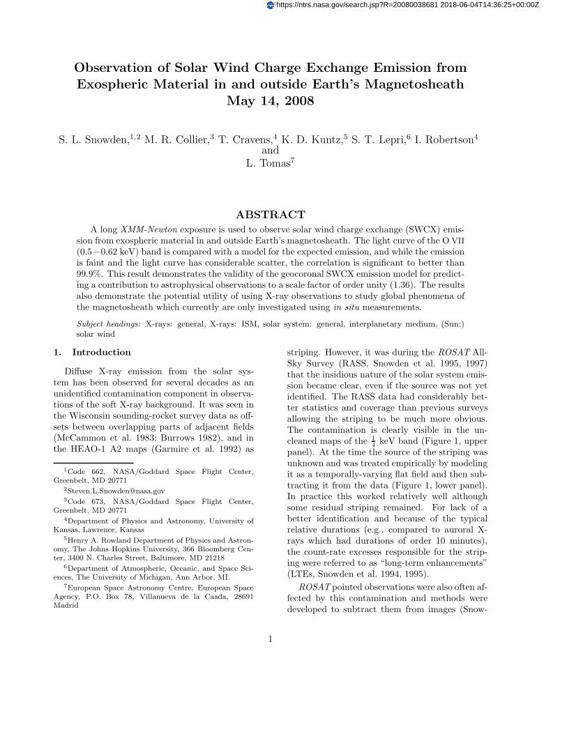
striping. However, it was during the ROSAT All-Sky Survey (RASS, Snowden et al. 1995, 1997)that the insidious nature of the solar system emis-sion became clear, even if the source was not yetidentified. The RASS data had considerably bet-ter statistics and coverage than previous surveysallowing the striping to be much more obvious.The contamination is clearly visible in the un-cleaned maps of the 1

4 keV band (Figure 1, upperpanel). At the time the source of the striping wasunknown and was treated empirically by modelingit as a temporally-varying flat field and then sub-tracting it from the data (Figure 1, lower panel).In practice this worked relatively well althoughsome residual striping remained. For lack of abetter identification and because of the typicalrelative durations (e.g., compared to auroral X-rays which had durations of order 10 minutes),the count-rate excesses responsible for the strip-ing were referred to as “long-term enhancements”(LTEs, Snowden et al. 1994, 1995).

ROSAT pointed observations were also often af-fected by this contamination and methods weredeveloped to subtract them from images (Snow-

1

https://ntrs.nasa.gov/search.jsp?R=20080038681 2018-06-04T14:36:25+00:00Z

den et al. 1994). One such observation is of par-ticular interest, a pointing at the Moon (Schmittet al. 1991). The surface brightness of the darkside of the moon (the observation was done whenthe Moon was half full) was well above the levelexpected from known sources, and Schmitt et al.(1991) suggested that the excess emission wasbremsstrahlung from solar-wind electrons imping-ing on the surface. However, comparing the off-Moon intensity of the observation with the cleanedRASS data showed a significant excess likely dueto an LTE. In addition, the enhancement wasroughly equal to the surface brightness of the darkMoon, which suggests a cis-lunar origin for theLTEs.

The study of diffuse X-ray emission from thesolar system gained interest with the detection ofX-rays from comets (e.g., Lisse et al. 1996). Af-ter some discussion as to the origin of the X-rays(e.g., scattered solar X-rays were considered andthen ruled out) it was eventually determined thatsolar wind charge exchange (SWCX) was respon-sible (Cravens 1997). SWCX occurs when a highlycharged ion of the solar wind interacts with a neu-tral atom and picks up an electron in a highlyexcited state. The excited ion then decays to alower energy state emitting a photon with a char-acteristic energy of the ion.

SWCX was subsequently suggested as thesource mechanism for the LTEs observed in theRASS as well as ROSAT pointed observations(Cox 1998; Cravens 2000). Because of the timescales of their temporal variability measurable byROSAT (a few days or less) the location of theLTE production is likely to be relatively local inthe solar system; either from near Earth’s mag-netosheath or within the nearest few AU fromEarth.

SWCX has been observed by Chandra (e.g.,during a dark moon observation, Wargelin et al.2004), XMM-Newton (e.g., during an observationof the Hubble Deep Field North, HDFN, Snow-den, Collier, & Kuntz 2004, hereafter SCK04),and Suzaku (e.g., during an observation of thenorth ecliptic pole, Fujimoto et al. 2007). Whilethe SWCX emission observed by Chandra clearlymust originate in the near-Earth environment asthe pointing was at the dark Moon, that need notbe the case for the XMM-Newton and Suzaku ob-servations. Figure 1 of SCK04 displays the time

variation of the X-ray emission, solar wind flux,and oxygen ionization state ratios for that observa-tion while their Figures 2 and 3 show the observedspectrum of the SWCX emission. The spectrumshows strong lines of O VII and O VIII, as well aslines from C VI, Ne IX, and Mg XI, all of which arealso lines of astrophysical interest. The 0.52-0.75keV band light curve has a nearly constant rateuntil a strong solar wind enhancement (as mea-sured by the ACE spacecraft) passes the earth,and as the solar wind flux and ionization state (asmeasured by the O+7/O+6 ratio) drop, so doesthe X-ray count rate. On one hand, the nearlycontemporaneous cutoff suggests a near-Earth ori-gin for the SWCX. On the other hand, the nearlyconstant count rate before the drop, in spite ofthe large parameter variations, suggests otherwise.Distributing the SWCX emission over a longerpath length along the line of sight could smoothout the light curve, however Collier et al. (2005a)demonstrate that the emission would still have tooriginate over a small fraction of an AU. The sameevent has been modeled as due to a large scale he-liospheric structure (Koutroumpa et al. 2006), butthe bulk of the variation is due to local emission.On the third hand, the XMM-Newton observationgeometry was serendipitously good for observingSWCX emission from near the sub-solar point ofEarth’s magnetosheath. This is the region of max-imum exospheric emission (Robertson & Cravens2003), which again suggests a very local origin.

Although the event described by SCK04 por-trayed the full scale of the problem of the time-variable SWCX emission, it was not clear whetherthe emission was due primarily to the solar windinteraction with exospheric material in and justoutside the magnetosheath (a large emissivity overa fairly short path-length) or whether the emissionwas primarily due to the solar wind interactionwith neutral material in the heliosphere (a smalleremissivity over a much longer path-length). Anarchival study of sets of repeated XMM-Newtonobservations of the same target showed that timevariable SWCX can be a problem even when one isnot observing near the sub-solar point of the mag-netosheath, provided that the solar wind flux isrelatively high (Kuntz & Snowden 2008a). This ismade clear by ROSAT and Suzaku observationsbeing affected by SWCX as both observatorieswere/are only able to observe through the flanks

2

of the magnetosheath. (Both satellites had/haveorbits with altitudes of 550–600 km and were con-strained to observe within a range of ∼ ±20◦ fromthe perpendicular to the Earth-Sun line.) How-ever, the Kuntz & Snowden (2008a) study did notresolve the question of the importance of the mag-netospheric origin of the time variable SWCX.

For the fifth XMM-Newton Announcement ofOpportunity (AO-5) we proposed for and receiveda 100 ks time critical observation (composed ofboth Guest Observer and calibration time) allow-ing us to set the geometry of the pointing to max-imize the observed flux from the magnetosheath.Despite our best endeavors, and the sterling effortsof the XMM-Newton Science Operations Center(SOC), we were unable to schedule an enhance-ment of the solar wind flux at the time of the ob-servation to improve our statistics. However, evenwith a moderate solar wind flux we were able toidentify a significant correlation between the O VII

count rate and our model for SWCX emission fromthe near-Earth environment. We were also able touse the observation to extract the line intensitiesfor O VII and O VIII emission by spectral fitting.

The goal of this observation was to verify andcalibrate our model for SWCX emission fromexospheric material in or outside Earth’s mag-netosheath in order to better model and pre-dict what, for astrophysical observations, is oc-casionally a significant background component.This significance was recently made very clearby the case of the disappearing warm-hot inter-galactic medium (WHIM) near the Coma clus-ter. Finoguenov, Briel, & Henry (2003) identi-fied excess O VII, O VIII, and Ne IX emission inone observation of the many XMM-Newton ComaCluster observations, and this excess emission wasattributed to the WHIM. However, a recent paperby Takei et al. (2008) using Suzaku data from thesame direction on the sky show no evidence forthe excess emission. While the solar wind wasin a relatively quiescent state during the XMM-Newton observation we note that the observationgeometry was similar to the 2001 HDFN observa-tion of SCK04 which showed very strong SWCXemission.

Section 2 of this paper describes the X-ray data,observation geometry, and ACE solar-wind data,§ 3 describes our model for the magnetosheathand near-Earth SWCX emission, § 4 describes our

analysis, and § 5 discusses our results and conclu-sions.

2. Data and Observation Geometry

2.1. X-ray Data

The X-ray data used for this study came froma single continuous observation obtained withXMM-Newton (Jansen et al. 2001; Ehle et al.2005) during AO-5, ObsID 0402530201. Table 1contains the observation and line-of-sight (LOS)details. The observation took place on 2006 June4-5 and lasted ∼ 96.4 ks. The European PhotonImaging Camera (EPIC) detectors (Turner et al.2001) were operated in their Full-Frame (MOS1and MOS2) and Extended Full Frame (pn) modeswith medium filters for the MOS detectors andthe thin filter for the pn. The observation was rel-atively unaffected by the soft-proton background(see Kuntz & Snowden 2008a). The data wereprocessed with XMM-Newton Science AnalysisSoftware (SAS1) Version 7.1.2 using the CurrentCalibration Files (CCF) available on 2008 March12.

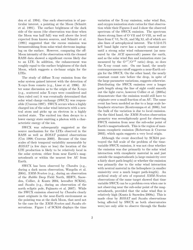
The data were reduced using the methods out-lined in Snowden et al. (2008), which includedrunning the tasks emchain and epchain to createcalibrated photon event files for the EPIC MOSand pn detectors, respectively. espfilt was usedto filter the data to remove times of soft-protoncontamination for the spectral analysis. Figure 2shows the MOS1 espfilt diagnostic plot with the2.5–12.0 keV light curve from the field of view(FOV), the 2.5–12.0 keV light curve from the un-exposed pixels (pixels in the corners of the de-tector that are not exposed to the sky), and thehistogram of the values in the FOV light curve.The diagnostic plots for the MOS2 and pn instru-ments are very similar. Spectra were extractedfrom the entire FOV of the MOS data after remov-ing point sources detected to a uniform limit of2× 10−15 ergs cm−2 s−1 and data from CCDs op-erating in an anomalous state (Kuntz & Snowden2008a). For each point source, the excluded regioncontains 90% of the emission due to the source,so the size of the excluded region varies with thesource’s intensity and distance from the optical

1http://xmm.esac.esa.int/external/xmm sw cal/sas frame.shtml

3

axis. The XMM-ESAS2 software (Snowden &Kuntz 2006; Snowden et al. 2008) was used to cre-ate model quiescent particle background spectra(Kuntz & Snowden 2008a). We did not extracta spectrum from the EPIC pn data as we havenot yet developed a suitable background model forthat detector.

We used data from all three instruments forthe light-curve analysis. We extracted light curvesin the energy ranges 0.50–0.61 keV (for an O VII

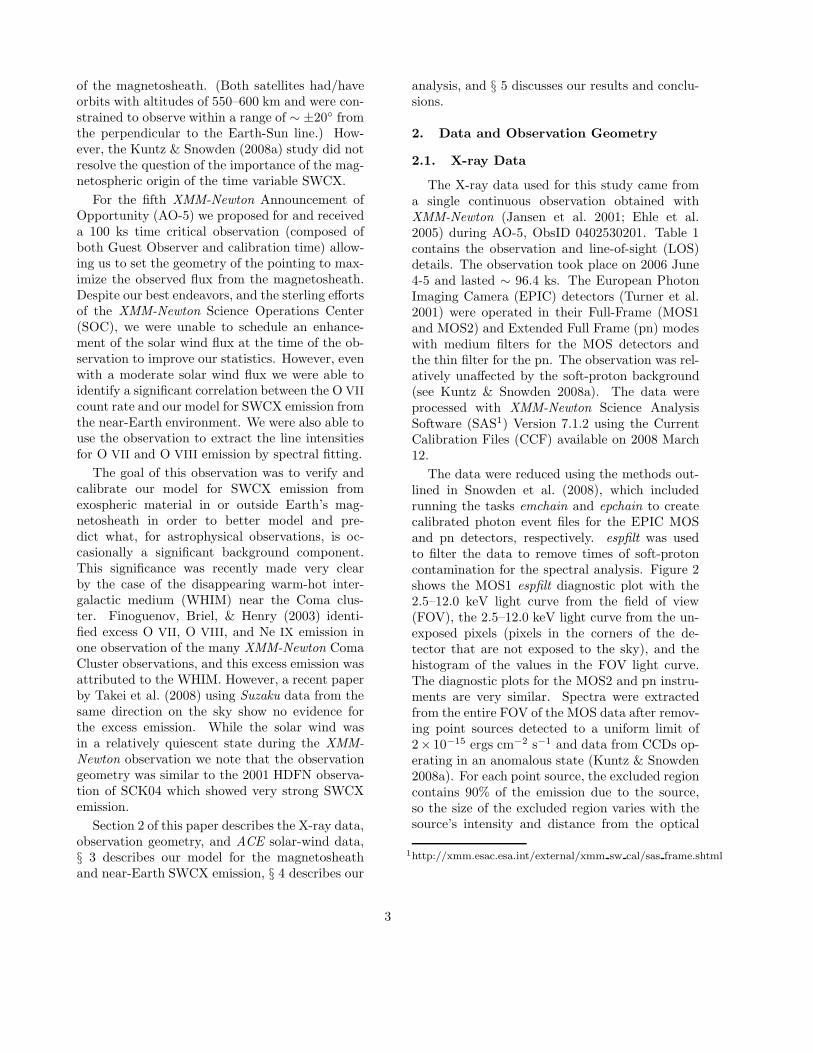
band) and 2.5–12.0 keV (a soft-proton monitoringband) from the MOS1 and MOS2 detectors andlight curves in the 0.45–0.65 keV and 2.5–12.0 keVbands were extracted from the pn (the broaderO VII band for the pn was required by the slightlylower energy resolution). Scatter plots were cre-ated of the O VII band versus the hard band (Fig-ure 3). For all of the detectors the bulk of the datapoints are strongly clumped, while the outliers arelinearly correlated. Since the soft proton spectrumhas a roughly power-law spectral shape affectingthe entire XMM-Newton EPIC energy range, thislinear correlation implies that the outliers are dueto increased soft proton contamination. The countrates from all detectors were added together afterexcluding the outliers, i.e., those points not in theclumps in Figure 3. Only time periods with ac-cepted count rates from all three detectors wereincluded in the light-curve analysis.

2.2. Observation Geometry

The geometry for this observation had severalconstraints. First, in order to maximize the ob-served SWCX emission from the magnetosheath,the look direction was required to sweep throughthe subsolar point, which is about 10 Re (Earthradii) toward the Sun along the Earth-Sun lineduring typical solar wind conditions. The sweep-ing was accomplished by fixing the pointing direc-tion for the observation so that the motion of thesatellite in its orbit would properly position theline of sight so it cut through the magnetosheathin the desired manner. Because XMM-Newton’sapogee distance is also ∼ 10 Re and XMM-Newtonis only able to point within ±20◦ of the perpen-dicular from the Earth-Sun line, we required anobservation date for which the apogee was nearthe Earth-Sun line (early June). While there was

2http://xmm.gsfc.nasa.gov/docs/xmm/xmmhp xmmesas.html

no reason to point at any specific position on thesky, in order to maximize the ratio of the SWCXemission to the cosmic background we needed tochoose a direction on the sky where the cosmicbackground is faint in the 3

4 keV band.After a somewhat painful period of trial and

error we were able to find an orbit and lookdirection which satisfied the constraints; revolu-tion (orbit) #1188, 2006 June 4–5 with α =22hr19m45.30s, δ = +72◦26′22.0′′. The Galac-tic column density of H I in this direction is∼ 3×1021 cm−2 and the RASS 3

4 keV count rate is∼ 8×10−5 counts s−1 arcmin−2, a very low countrate. The RASS 1

4 keV emission is also quite lowin this direction. Figures 4 and 5 detail the obser-vation geometry of the satellite location and lookdirection relative to the magnetosheath.

2.3. The Solar Wind and ACE Data

The solar wind, a partially ionized plasma con-tinually flowing from the Sun, contains on averageabout 96% protons, 4% alpha particles, and lessthan one percent heavier highly charged species.Solar wind densities are typically ∼ 5 cm−3 andthe magnetic field strength is about 7 nT. How-ever, solar wind properties are highly time vari-able, and over the approximately eleven year so-lar cycle the solar wind flux goes from an averageof about 3.2 × 108 cm−2 s−1 at solar minimum toabout 4.8×108 cm−2 s−1 at solar maximum, whilethe solar wind speed goes from about 390 km s−1

at solar minimum to 530 km s−1 at solar maxi-mum (Rucinski et al. 1996). The solar wind tendsto be highly structured with scale lengths as shortas tens of Earth radii in both the magnetic field(Collier et al. 1998) and plasma (Richardson &Paularena 2001). At the nominal flow speed ofabout 450 km s−1, the solar wind takes almostfour days to flow from the Sun to the Earth andover a year to arrive at at the termination shockat ∼ 100 AU.

Spacecraft such as the Advanced CompositionExplorer (ACE, Stone et al. 1998) and Wind(Acuna et al. 1995) monitor the solar wind fromthe L1 point, a point about 235 Earth radii up-stream where the gravitational force between theEarth and Sun balance. Because spacecraft at L1typically have halo orbits around this point witha radius of about 40 Earth radii, the in-situ ob-servations made by upstream monitors may not

4

reflect the exact properties of the solar wind thatimpacts Earth (or another spacecraft) and thereis a non-negligible lag (∼ 1 hour between L1 andthe Earth.)

The small fraction of heavy high charge-stateions in the solar wind produces the soft X-rayemission from SWCX. Unfortunately, because oftheir low abundance in the solar wind, measure-ments of these minor ion species require special in-strumental techniques (e.g., Gloeckler et al. 1995),and so are more limited than measurements of theproton and alpha particle densities, flow speeds,and temperatures.

During solar minimum, when most XMM-Newton observations have occurred, the solar windas observed at Earth has shown a periodic struc-ture, oscillating between fast polar coronal holeflow and slower interstream flow as the Sun and itssolar dipole rotate. This behavior is relatively typ-ical for observations near solar minimum. At thetime of the XMM-Newton observation, as shownin Figure 6, the solar wind flux measured by theACE spacecraft was usually below its nominal fluxof 3× 108 cm−2 s−1. The two-hour-averaged O+7

flux, also from ACE, showed relatively typical val-ues. In short, this was a calm solar wind timeperiod.

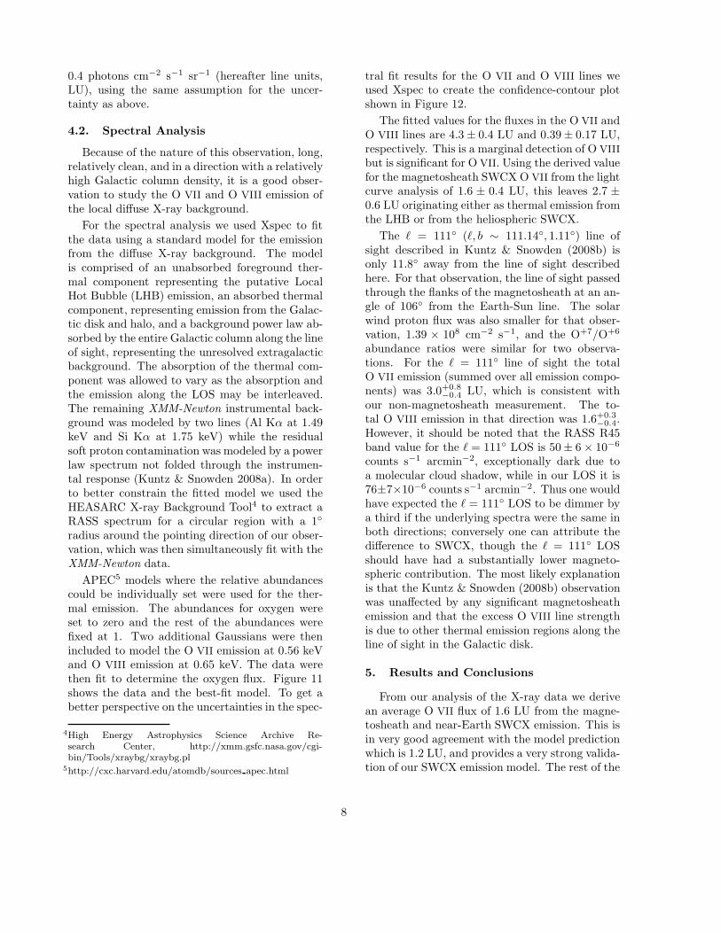
To give a perspective on the solar wind fluxesduring the time of the X-ray observation, Figure 7shows the integral histograms of the solar windproton and O+7 fluxes for the year 2006. Therange of proton fluxes were typical for the yearwhile on average the O+7 fluxes were slightly ele-vated.

3. Magnetosheath SWCX Emission Model

SWCX emission is due to the transfer of an elec-tron from a neutral atom, usually H or He, to anexcited state in a heavy solar wind ion, and thesubsequent radiative decay. Given the ionizationstates in the solar wind, the resultant photons aretypically in the extreme UV or soft X-ray regionof the spectrum. Following Cravens (2000) we de-fine the photon production rate (emissivity) for agiven line as:

PX = αnswnn〈g〉 (1)

where nsw is the density of the solar wind protons,nn is the density of the neutral “donor” atoms, and

< g > is their relative velocity. The scale factor αcontains the abundance of the solar wind ion of in-terest, the branching ratios in the radiative decay,and the interaction cross-section, which dependsupon the relative velocity, and the donor species.For hydrogen and for medium solar wind activity,a reasonable value for an α appropriate for a broadX-ray band with E> 100 eV is 6 × 10−16 eV cm2

(Pepino et al. 2004), and for helium the value isabout half that of hydrogen.

The total X-ray emission observed from a spe-cific line of sight is given by

4πI =∫ s=∞

s=0

PX(s)ds (2)

where s is the position along the line of sight. Theinterval over which one needs to integrate is set bythe phenomena producing the emission.

For a line of sight originating from a space-craft in earth orbit there are two sources of neu-tral donor atoms. The first is the extended geo-corona, the outermost, most tenuous part of theatmosphere, which is composed almost entirely ofhydrogen. The geocoronal neutral densities areobtained from the Hodges (1994) model of the ter-restrial exospheric hydrogen density. This modelis tabulated to 9.7 RE , where the structure isfairly smooth; we have extrapolated the modelat higher R with a R−3 distribution. The sec-ond source of donor atoms, which is spatially quitecomplex, is the neutral interstellar medium whichstreams through the heliosphere. The interstel-lar medium is comprised primarily of H and Hewhere the density of He is about 10% that of Hin the local interstellar cloud (LIC) which sur-rounds the heliosphere (Gloeckler & Geiss 2001;Gloeckler et al. 2004). The interstellar mediumwithin the heliosphere is initially the same butis strongly affected by the Sun. As interstellaratomic hydrogen approaches the Sun it experi-ences both the attractive force of gravity (∝ r−2)and the repulsive force of radiation pressure (also∝ r−2). This creates a hydrogen cavity aroundthe Sun with a radius (at the 10% density level)of a few AU in the up-interstellar-wind direction(λ, β ∼ 254◦ ± 3◦, 7◦ ± 3◦) to ∼ 10 − 15 AU inthe downstream direction (Quemerais, Lallement,& Bertaux 1993). Because hydrogen is also ion-ized as it approaches the Sun, its upwind den-sity is significantly greater than its downwind den-

5

sity. Neutral helium is also depleted near the Sundue to photoionization, however because the crosssections for helium are significantly smaller thanthose for hydrogen, helium can be found muchcloser to the Sun than hydrogen. Further, asneutral helium passes the Sun, it is gravitation-ally focused, substantially increasing its densityin the downwind helium-focusing cone. We havederived the interstellar neutral densities from theFahr “hot” model (Fahr 1971, 1974).

There are two important regimes for solar windion-neutral interactions. The first is the magne-tosheath, the region directly behind the Earth’sbowshock. The bowshock brakes the solar wind,increasing the density of the solar wind in the“nose” of the bowshock by roughly a factor of four,and by lower factors along the “flanks” of the bow-shock. Since the nose of the magnetosheath is alsothe place where the bowshock is the closest to theEarth, this is also the magnetosheath region withthe highest neutral density, and thus the region ex-pected to have the greatest SWCX emission. Thesolar wind parameters (density, speed, and tem-perature) inside the magnetosheath are given bythe Spreiter, Sumers, & Alksne (1966) numericalglobal hydrodynamic model. The second regime ofinterest is the free space outside of the bowshock.Here there is still a significant density of geocoro-nal hydrogen as well as the free-flowing interstellarmedium.

The nose of the magnetopause is at ∼ 9.7 RE

under nominal solar wind conditions, and that dis-tance varies with the solar wind ram pressure as(nswu2

sw

)− 16 , where usw is the solar wind speed.

Because the exospheric density drops off as R−3

where R is distance from the center of the Earth,the exospheric neutral density at the nose of themagnetopause varies as ∼ R−3 ∼ (nswu2

sw)−12 .

The soft X-ray emission scales with the product ofthe exospheric neutral density and the solar windflux, nswusw, so that the soft X-ray emission goesas ∼ nswusw(nswu2

sw)−12 = n

32swu2

sw. The emis-sion responds non-linearly to both increases in so-lar wind density and solar wind speed varying al-most as the square of the solar wind flux. Withthis observation taking place during a relative lullin the solar wind, the expected SWCX emission isalso relatively low.

We have integrated our model for the interac-

tion of the solar wind with the geocoronal neutralmaterial, including the interactions in the magne-tosheath to a distance of 50 RE . We have inte-grated our model for the interaction of the solarwind with the interstellar material to a distance of200 AU; essentially encompassing the entire pathlength through the heliosphere.

The solar wind conditions enter our model notonly through the nsw in Equation 1 and throughthe α in Equation 1, which depends on the veloc-ity and temperature of the solar wind, but alsothrough the Spreiter, Sumers, & Alksne (1966)model of the magnetosheath since the size andshape of the magnetosheath depends upon thestrength of the solar wind. We have modeled thesolar wind as a series of spherical fronts emanat-ing from the Sun. The solar wind proton density,speed, and temperature for each front was derivedfrom the OMNIWeb3 archive. The data extractedfrom OMNIWeb (King & Papitashvili 2004) hada time resolution of one hour, and the data weretime shifted to the location of the bowshock. Theproton thermal velocity was derived from the pro-ton temperature using

vth =√

3kBT/mp, (3)

where mp is the proton mass and T is the protontemperature, while the total average proton speedwas calculated using

〈g〉 =√

v2th + u2

sw (4)

where usw is the measured average proton speed.As discussed above, the interaction of the so-

lar wind with the magnetosheath causes mag-netosheath to expand and contract. With eachtime step we scale the Spreiter, Sumers, & Alk-sne (1966) model of the magnetosheath to the sizeapropriate for the solar wind flux in that time step,and then integrate the emissivity along the lineof sight. Given the limitations of the solar winddata, we assume nearly planar propagation nearthe earth and a uniform pressure across the nose ofthe magnetosheath. Such treatment is valid giventhe time-scales involved; due to low count ratesthe X-ray data require a time binning of 15 min-utes to achieve a reasonable significance while the

3http://omniweb.gsfc.nasa.gov/

6

time required for a solar wind front to move fromthe nose of the magnetosheath to the level of theearth is only about three minutes. Thus, muchof the dynamic nature of the magnetosheath willbe averaged out by the time-binning forced by theX-ray data.

4. Analysis

4.1. Light Curve

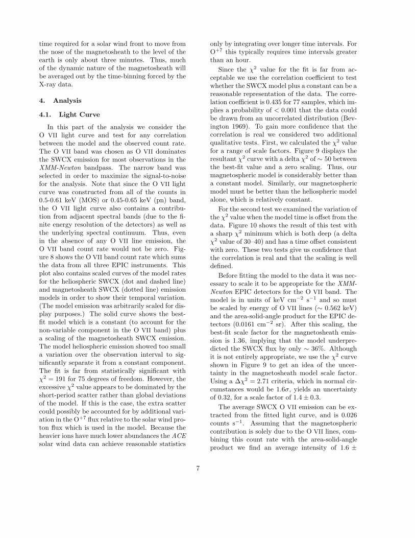
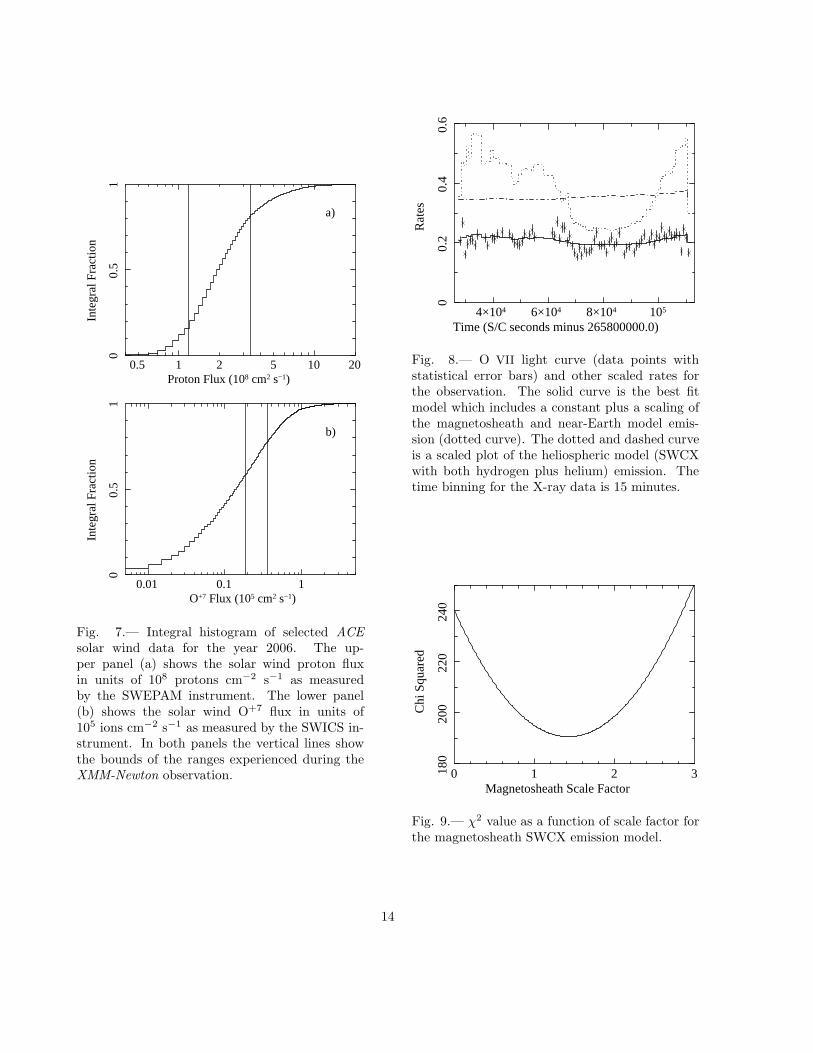
In this part of the analysis we consider theO VII light curve and test for any correlationbetween the model and the observed count rate.The O VII band was chosen as O VII dominatesthe SWCX emission for most observations in theXMM-Newton bandpass. The narrow band wasselected in order to maximize the signal-to-noisefor the analysis. Note that since the O VII lightcurve was constructed from all of the counts in0.5-0.61 keV (MOS) or 0.45-0.65 keV (pn) band,the O VII light curve also contains a contribu-tion from adjacent spectral bands (due to the fi-nite energy resolution of the detectors) as well asthe underlying spectral continuum. Thus, evenin the absence of any O VII line emission, theO VII band count rate would not be zero. Fig-ure 8 shows the O VII band count rate which sumsthe data from all three EPIC instruments. Thisplot also contains scaled curves of the model ratesfor the heliospheric SWCX (dot and dashed line)and magnetosheath SWCX (dotted line) emissionmodels in order to show their temporal variation.(The model emission was arbitrarily scaled for dis-play purposes.) The solid curve shows the best-fit model which is a constant (to account for thenon-variable component in the O VII band) plusa scaling of the magnetosheath SWCX emission.The model heliospheric emission showed too smalla variation over the observation interval to sig-nificantly separate it from a constant component.The fit is far from statistically significant withχ2 = 191 for 75 degrees of freedom. However, theexcessive χ2 value appears to be dominated by theshort-period scatter rather than global deviationsof the model. If this is the case, the extra scattercould possibly be accounted for by additional vari-ation in the O+7 flux relative to the solar wind pro-ton flux which is used in the model. Because theheavier ions have much lower abundances the ACEsolar wind data can achieve reasonable statistics

only by integrating over longer time intervals. ForO+7 this typically requires time intervals greaterthan an hour.

Since the χ2 value for the fit is far from ac-ceptable we use the correlation coefficient to testwhether the SWCX model plus a constant can be areasonable representation of the data. The corre-lation coefficient is 0.435 for 77 samples, which im-plies a probability of < 0.001 that the data couldbe drawn from an uncorrelated distribution (Bev-ington 1969). To gain more confidence that thecorrelation is real we considered two additionalqualitative tests. First, we calculated the χ2 valuefor a range of scale factors. Figure 9 displays theresultant χ2 curve with a delta χ2 of ∼ 50 betweenthe best-fit value and a zero scaling. Thus, ourmagnetospheric model is considerably better thana constant model. Similarly, our magnetosphericmodel must be better than the heliospheric modelalone, which is relatively constant.

For the second test we examined the variation ofthe χ2 value when the model time is offset from thedata. Figure 10 shows the result of this test witha sharp χ2 minimum which is both deep (a deltaχ2 value of 30–40) and has a time offset consistentwith zero. These two tests give us confidence thatthe correlation is real and that the scaling is welldefined.

Before fitting the model to the data it was nec-essary to scale it to be appropriate for the XMM-Newton EPIC detectors for the O VII band. Themodel is in units of keV cm−2 s−1 and so mustbe scaled by energy of O VII lines (∼ 0.562 keV)and the area-solid-angle product for the EPIC de-tectors (0.0161 cm−2 sr). After this scaling, thebest-fit scale factor for the magnetosheath emis-sion is 1.36, implying that the model underpre-dicted the SWCX flux by only ∼ 36%. Althoughit is not entirely appropriate, we use the χ2 curveshown in Figure 9 to get an idea of the uncer-tainty in the magnetosheath model scale factor.Using a Δχ2 = 2.71 criteria, which in normal cir-cumstances would be 1.6σ, yields an uncertaintyof 0.32, for a scale factor of 1.4 ± 0.3.

The average SWCX O VII emission can be ex-tracted from the fitted light curve, and is 0.026counts s−1. Assuming that the magnetosphericcontribution is solely due to the O VII lines, com-bining this count rate with the area-solid-angleproduct we find an average intensity of 1.6 ±

7

0.4 photons cm−2 s−1 sr−1 (hereafter line units,LU), using the same assumption for the uncer-tainty as above.

4.2. Spectral Analysis

Because of the nature of this observation, long,relatively clean, and in a direction with a relativelyhigh Galactic column density, it is a good obser-vation to study the O VII and O VIII emission ofthe local diffuse X-ray background.

For the spectral analysis we used Xspec to fitthe data using a standard model for the emissionfrom the diffuse X-ray background. The modelis comprised of an unabsorbed foreground ther-mal component representing the putative LocalHot Bubble (LHB) emission, an absorbed thermalcomponent, representing emission from the Galac-tic disk and halo, and a background power law ab-sorbed by the entire Galactic column along the lineof sight, representing the unresolved extragalacticbackground. The absorption of the thermal com-ponent was allowed to vary as the absorption andthe emission along the LOS may be interleaved.The remaining XMM-Newton instrumental back-ground was modeled by two lines (Al Kα at 1.49keV and Si Kα at 1.75 keV) while the residualsoft proton contamination was modeled by a powerlaw spectrum not folded through the instrumen-tal response (Kuntz & Snowden 2008a). In orderto better constrain the fitted model we used theHEASARC X-ray Background Tool4 to extract aRASS spectrum for a circular region with a 1◦

radius around the pointing direction of our obser-vation, which was then simultaneously fit with theXMM-Newton data.

APEC5 models where the relative abundancescould be individually set were used for the ther-mal emission. The abundances for oxygen wereset to zero and the rest of the abundances werefixed at 1. Two additional Gaussians were thenincluded to model the O VII emission at 0.56 keVand O VIII emission at 0.65 keV. The data werethen fit to determine the oxygen flux. Figure 11shows the data and the best-fit model. To get abetter perspective on the uncertainties in the spec-

4High Energy Astrophysics Science Archive Re-search Center, http://xmm.gsfc.nasa.gov/cgi-bin/Tools/xraybg/xraybg.pl

5http://cxc.harvard.edu/atomdb/sources apec.html

tral fit results for the O VII and O VIII lines weused Xspec to create the confidence-contour plotshown in Figure 12.

The fitted values for the fluxes in the O VII andO VIII lines are 4.3 ± 0.4 LU and 0.39 ± 0.17 LU,respectively. This is a marginal detection of O VIII

but is significant for O VII. Using the derived valuefor the magnetosheath SWCX O VII from the lightcurve analysis of 1.6 ± 0.4 LU, this leaves 2.7 ±0.6 LU originating either as thermal emission fromthe LHB or from the heliospheric SWCX.

The = 111◦ (, b ∼ 111.14◦, 1.11◦) line ofsight described in Kuntz & Snowden (2008b) isonly 11.8◦ away from the line of sight describedhere. For that observation, the line of sight passedthrough the flanks of the magnetosheath at an an-gle of 106◦ from the Earth-Sun line. The solarwind proton flux was also smaller for that obser-vation, 1.39 × 108 cm−2 s−1, and the O+7/O+6

abundance ratios were similar for two observa-tions. For the = 111◦ line of sight the totalO VII emission (summed over all emission compo-nents) was 3.0+0.8

−0.4 LU, which is consistent withour non-magnetosheath measurement. The to-tal O VIII emission in that direction was 1.6+0.3

−0.4.However, it should be noted that the RASS R45band value for the = 111◦ LOS is 50 ± 6 × 10−6

counts s−1 arcmin−2, exceptionally dark due toa molecular cloud shadow, while in our LOS it is76±7×10−6 counts s−1 arcmin−2. Thus one wouldhave expected the = 111◦ LOS to be dimmer bya third if the underlying spectra were the same inboth directions; conversely one can attribute thedifference to SWCX, though the = 111◦ LOSshould have had a substantially lower magneto-spheric contribution. The most likely explanationis that the Kuntz & Snowden (2008b) observationwas unaffected by any significant magnetosheathemission and that the excess O VIII line strengthis due to other thermal emission regions along theline of sight in the Galactic disk.

5. Results and Conclusions

From our analysis of the X-ray data we derivean average O VII flux of 1.6 LU from the magne-tosheath and near-Earth SWCX emission. This isin very good agreement with the model predictionwhich is 1.2 LU, and provides a very strong valida-tion of our SWCX emission model. The rest of the

8

observed O VII emission, 2.7 LU, originates fore-ground to the dark clouds forming the backstopfor this observation, and so may originate in theheliosphere, LHB, or farther away in the Galacticdisk. This value agrees reasonably well with the3.0 LU results of Kuntz & Snowden (2008b) andthe 3.5 LU local emission of Smith et al. (2007).

Our marginal O VIII result of 0.4 LU is sig-nificantly lower than those of Kuntz & Snowden(2008b) but agrees well with the marginal local re-sult of Smith et al. (2007) (0.24 ± 0.10 LU). Thisplaces an upper limit on O VIII SWCX emissionfrom the heliosphere, which should be relativelyconstant over time, of ∼ 0.3 LU.

With a functional model for SWCX emissionfrom the magnetosheath and near-Earth environ-ment it is now possible to identify those astrophys-ical observations which are likely to be affected bythis “contamination” component. With further re-finements of the model and additional calibrationobservations it may be possible to model SWCXemission accurately enough to subtract it from thedata.

Another interesting possibility suggested by thesuccess of this project is the remote monitoringof the magnetosheath, magnetopause, and solarwind. In the past, observations of the terrestrialmagnetopause have been mainly restricted to in-situ observations. The notable exceptions to thisare neutral atom imaging (e.g., Taguchi et al. 2004;Collier et al. 2005b) and radio plasma imaging(e.g., Green & Reinisch 2003; Nagano et al. 2003).X-ray imaging, however, may be the best tech-nique for global monitoring of the magnetopausefrom, for example, a spacecraft positioned off tothe side of the Earth in a 1 AU orbit that leadsor follows the Earth, viewing nearly perpendicu-lar to the Earth-Sun line (Robertson & Cravens2003; Robertson et al. 2006). Given that all en-ergy transfer from the solar wind into the mag-netosphere must pass through the magnetopause,global imaging of the magnetopause boundary willprove invaluable for space weather studies.

We would like to thank the mission plannersat the XMM-Newton Science Operations Center(SOC) for their patience and help in the schedul-ing of this non-standard time-critical observation.We would also like to thank the SOC for the addi-tional Calibration Time that was allocated to the

observation.This paper was based on an observation ob-

tained with XMM-Newton, an ESA science mis-sion with instruments and contributions directlyfunded by ESA Member States and NASA. TheOMNI data were obtained from the GSFC/SPDFOMNIWeb interface. This work was supportedby a NASA XMM-Newton GO grants includingNNX06AG73G.

REFERENCES

Acuna, M. H., Ogilvie, K. W., Baker, D. N., Cur-tis, S. A., Fairfield, D. H., & Mish, W. H. 1995,Space Sci. Rev., 71, 5

Bevington, P. R. 1969, Data Reduction and ErrorAnalysis for the Physical Sciences, (McGraw-Hill Book Company:New York)

Burrows, D. N. 1982, Ph.D. Thesis, Universityof Wisconsin-Madison, Spatial structure of thediffuse soft X-ray background

Collier, M. R., Slavin, J. A., Lepping, R. P., Szabo,A., & Ogilvie, K. 1998, Geophys. Res. Lett., 25,2509

Collier, M. R., Moore, T. E., Snowden, S. L., &Kuntz, K. D. 2005, Adv. Space Res., 35(12),2157

Collier, M. R., Moore, T. E., Fok, M.-C., Pilker-ton, B., Boardsen, S., Khan, H. 2005, J. Geo-phys. Res., 110, A02102

Cox, D. P. 1998, in The Local Bubble and Be-yond, ed. D. Breitschwerdt, M. J. Freyberg, &J. Trmper (Berlin: Springer), 121

Cravens, T. E. 1997, Geophys. Res. Lett., 24, 105

Cravens, T. E. 2000, ApJ, 532, L153

Ehle, M., et al. 2005, XMM-Newton Users’ Hand-book (Madrid:ESA)

Fahr, H. J. 1971, A&A, 14 263

Fahr, H. J. 1974, Sp. Science Rev., 15, 483

Finoguenov, A., Briel, U. G., & Henry, J. P. 2003,A&A, 410, 777

9

Fujimoto, R., Mitsuda, K., McCammon, D.,Takei, Y., Bauer, M., Ishisaki, Y., Porter, S. F.,Yamaguchi, H., Hayashida, K., & Yamasaki,N. Y. 2007, PASJ, 59(SP1), 133

Garmire, G. P., Nousek, J. A., Apparao, K. M. V.,Burrows, D. N., Fink, R. L., & Kraft, R. P.1992, ApJ, 399, 694

Gloeckler, G., & Geiss, J. 2001, AIP Conf. Proc.598, Solar and Galactic Composition, ed. R. F.Wimmer-Schweingruber (New York: AIP), 281

Gloeckler, 1995, Space Sci. Rev., 71, 79

Gloeckler, G., et al. 1998, SSRv, 86(1/4), 497

Gloeckler, G., et al. 2004, A&A, 426(3), 845

Green, J. L., & Reinisch, B. W. 2003, Space Sci.Rev., 109, 183

Hodges Jr., R. R. 1994, JGR, 99, 23, 229

Jansen, F., Lumb, D., Altieri, B., Clavel, J., Ehle,M., Erd, C., Gabriel, C., Guainazzi, M., Gon-doin, P., Much, R., Munoz, R., Santos, M.,Schartel, N., Texier, D., & Vacanti, G. 2001,A&A, 365, L1

King, J. H., & Papitashvili, N. E. 2004, JGR, 110,A2, A02209, 10.1029/2004JA010804

Koutroumpa, D., Lallement, R., Kharchenko, V.,Dalgarno, A., Pepino, R., Izmodenov, V., &Quemerais, E. 2006, A&A 460, 289

Kuntz, K. D., & Snowden, S. L. 2008a, A&A, 478,575

Kuntz, K. D., & Snowden, S. L. 2008b, ApJ, 674,209

Lisse, C. M., et al. 1996, Science, 274, 205

McCammon, D., Burrows, D. N., Sanders, W. T.,& Kraushaar, W. L. 1983, ApJ, 269, 107

McComas, D. J., Bame, S. J., Barker, P., Feldman,W. C., Phillips, J. L., Riley, P., & Griffee, J. W.1998, SSRv, 86(1/4), 563

Nagano, I., Wu, X.-Y., Takano, H., Yagitani, S.,Matsumoto, H., Hashimoto, K., Kasaba, Y.2003, J. Geophys. Res., 108, 1224

Pepino R., Kharchenko, V., Dalgarno, A. & Lalle-ment, R. 2004, ApJ, 617, 1347

Plucinsky, P. P., Snowden, S. L., Briel, U. G.,Hasinger, G., & Pfeffermann, E. 1993, ApJ,418, 519

Quemerais, E., Lallement, R., & Bertaux, J.-L.1993, J. Geophys. Res., 98, 15199

Richardson, J., & Paularena, K. 2001, J. Geophys.Res., 106, 239

Robertson, I. P., & Cravens, T. E. 2003, Geophys.Res. Lett., 30(8), 1439

Robertson, I. P., Collier, M. R., Cravens, T. E. &Fok, M.-C. 2006, JGR, 111, A12105

Rucinski, D., Cummings, A. C., Gloeckler, G.,Lazarus, A. J., Mobius, E., & Witte, M. 1996,Space Sci. Rev., 78, 73

Schmitt, J. H. M. M., Snowden, S. L., Aschenbach,B., Hasinger, G., Pfeffermann, E., Predehl, P.,& Trumper, J. 1991, Nature, 349, 583

Smith, R. K. et al. 2007, PASJ, 595(SP1), 141

Snowden, S. L., Collier, M. R., & Kuntz, K. D.2004, ApJ, 610, 1182

Snowden, S. L., & Freyberg, M. J. 1993, ApJ, 404,403

Snowden, S. L., Freyberg, M. J., Plucinsky, P. P.,Schmitt, J. H. M. M., Truemper, J., Voges,W., Edgar, R. J., McCammon, D., & Sanders,W. T. 1995, ApJ, 454, 643

Snowden, S. L., Egger, R., Freyberg, M. J., Mc-Cammon, D., Plucinsky, P. P., Sanders, W. T.,Schmitt, J. H. M. M., Trumper, J., & Voges,W. 1997, ApJ, 485, 125

Snowden, S. L., & Kuntz, K.D. 2006, XMM-Newton GOF,ftp://legacy.gsfc.nasa.gov/xmm/software/xmm-esas/xmm-esas.pdf

Snowden, S. L., McCammon, D., Burrows, D. N.,& Mendenhall, J. A., 1994, ApJ, 424, 714

Snowden, S. L., Mushtozky, R. F., Kuntz, K. D.,& Davis, D. S. 2008, A&A, 478, 615

10

Snowden, S. L., Plucinsky, P. P., Briel, U.,Hasinger, G., & Pfeffermann, E. 1992, ApJ,393, 819

Spreiter, J. R., Sumers, A. L., & Alksne, A. Y.1966, Space. Sci., 14, 223

Stone, E. C., Frandsen, A. M., Mewaldt, R. A.,Christian, E. R., Margolies, D., Ormes, J. F.,& Snow, F. 1998, SSRv, 86(1/4), 1

Taguchi, S., Collier, M. R., Moore, T. E., Fok, M.-C., Singer, H. J. 2004, J. Geophys. Res., 109,A04208

Takei, Y., Miller, E. D., Bregman, J. N., Kimura,S., Ohashi, T., Mitsuda, K., Tamura, T.,Yamasaki, N. Y, & Fujimoto, R. (2008),arXiv:0803.2817

Turner, M. J. L. et al. 2001, A&A, 365, L27

Wargelin, B. J., Markevitch, M., Juda, M.,Kharchenko, V., Edgar, R. J., & Dalgarno, A.2004, ApJ, submitted

This 2-column preprint was prepared with the AAS LATEXmacros v5.2.

0 0.0002 0.0004 0.0006 0.0008 0.001 0.0012 0.0014 0.0016 0.0018

Fig. 1.— RASS maps of the 14 keV dif-

fuse background before (upper panel) and af-ter (lower panel) removal of the LTEs. Thecolor bar shows the X-ray intensity in units ofcounts s−1 arcmin−2. The particle background(Snowden et al. 1992; Plucinsky et al. 1993)and scattered solar X-ray background (Snowden& Freyberg 1993) have been subtracted in bothmaps.

11

0 1 2 3 4 5

020

0040

0060

00

N

Count Rate (counts/s)

Count Rate Histogram Fit Limits: BlueSelection Limits: Red

0 2×104 4×104 6×104 8×1040.1

10.

20.

52

Cou

nt R

ate

(cou

nts/

s)

Time (s)

FOV Light Curve

0 2×104 4×104 6×104 8×104

00.

20.

40.

6

Cou

nt R

ate

(cou

nts/

s)

Time (s)

Corner Light Curve

Fig. 2.— MOS1 diagnostic plot from the SAStask espfilt with (upper panel) the histogram ofthe FOV 2.5–12.0 keV light curve, (middle panel)the 2.5–12.0 keV light curve from the FOV, and(lower panel) the 2.5–12.0 keV light curve fromthe unexposed (to the sky) corners of the detec-tor. Data plotted in green indicate accepted timeperiods. In the upper panel the vertical blue linesindicate the range over which the histogram datawere fitted with a Gaussian. The vertical red linesindicate the count rate range where the data wereaccepted.

0.5 1 1.5

00.

050.

10.

15

O V

II C

ount

Rat

e (c

ount

s −

1 ) MOS 1

0.5 1 1.5

00.

050.

10.

15

O V

II C

ount

Rat

e (c

ount

s −

1 )

2.5−12.0 keV Band Count Rate (counts s−1)

MOS 2

1 1.5 2 2.5 3 3.5

00.

20.

40.

6

O V

II C

ount

Rat

e (c

ount

s −

1 )

2.5−12.0 keV Band Count Rate (counts s−1)

PN

Fig. 3.— O VII band versus hard band count ratescatter plots for the MOS1 (upper panel), MOS2(middle panel), and pn (bottom panel) detectors.The plotted lines show the correlation between theoutliers indicating that both the hard band andO VII band are affected in a similar manner, fur-ther indicating that they are due to residual soft-proton contamination.

12

Fig. 4.— Geometry of the observation in theGSE X-Z plane, where X points to the Sun andZ points toward the north ecliptic pole. Thecurved solid line shows the XMM-Newton orbitduring the observation while the straight solidlines show the look direction. The dotted linesindicate the rough location of the inner and outerboundaries of Earth’s magnetosheath. The col-ored lines provide a rough estimate of the emis-sivity (nswnn〈g〉) within the magnetosheath. Theragged appearance of the boundary of the mag-netosheath emission is due the variability in thesolar wind strength.

Fig. 5.— Same as Figure 4 except that the projec-tion is in the GSE X-Y plane. The GSE Y axis liesin the ecliptic plane and points opposite to Earth’svelocity vector, completing the right-handed coor-dinate system.

155 160

110

100

1000

Para

met

er V

alue

Day of Year (2006)

Fig. 6.— ACE solar wind data for the obser-vation. The upper curve shows the solar windproton speed in units of km s−1 as measured bythe SWEPAM instrument (McComas et al. 1998).The middle curve is the O+7 flux in units of 102

ions cm−2 s−1 as measured by the SWICS instru-ment (Gloeckler et al. 1998). The bottom curveis the solar wind proton flux in units of 108 pro-tons cm−2 s−1 as measured by the SWEPAM in-strument. The vertical lines show the bounds ofthe XMM-Newton observation.

13

a)

1 100.5 2 5 20

00.

51

Inte

gral

Fra

ctio

n

Proton Flux (108 cm2 s−1)

b)

0.01 0.1 1

00.

51

Inte

gral

Fra

ctio

n

O+7 Flux (105 cm2 s−1)

Fig. 7.— Integral histogram of selected ACEsolar wind data for the year 2006. The up-per panel (a) shows the solar wind proton fluxin units of 108 protons cm−2 s−1 as measuredby the SWEPAM instrument. The lower panel(b) shows the solar wind O+7 flux in units of105 ions cm−2 s−1 as measured by the SWICS in-strument. In both panels the vertical lines showthe bounds of the ranges experienced during theXMM-Newton observation.

4×104 6×104 8×104 105

00.

20.

40.

6

Rat

es

Time (S/C seconds minus 265800000.0)

Fig. 8.— O VII light curve (data points withstatistical error bars) and other scaled rates forthe observation. The solid curve is the best fitmodel which includes a constant plus a scaling ofthe magnetosheath and near-Earth model emis-sion (dotted curve). The dotted and dashed curveis a scaled plot of the heliospheric model (SWCXwith both hydrogen plus helium) emission. Thetime binning for the X-ray data is 15 minutes.

0 1 2 3180

200

220

240

Chi

Squ

ared

Magnetosheath Scale Factor

Fig. 9.— χ2 value as a function of scale factor forthe magnetosheath SWCX emission model.

14

−2×104 0 2×104180

200

220

240

Chi

Squ

ared

Time Offset (s)

Fig. 10.— χ2 value as a function of time shift be-tween the magnetosheath SWCX emission modeland data.

10−

410

−3

0.01

0.1

1

Flux

(co

unts

s−

1 keV

−1 )

0.1 10.2 0.5 2

00.

51

1.5

2

Rat

io

Energy (keV)

Fig. 11.— Spectral fit for the XMM-Newton EPICMOS (white and red) and RASS (green) spectra.The two lines between 1.5 and 2.0 keV are theAl Kα and Si Kα instrumental lines. The O VII

line is at 0.56 keV. The O VIII line is not apparent.

2×10−7 4×10−7 6×10−7

02×

10−

84×

10−

86×

10−

88×

10−

810

−7

O V

III

Nor

mal

izat

ion

O VII Normalization

Fig. 12.— χ2 contour plot. The axis values arethe Xspec normalizations which are in units ofcounts s−1 arcmin−2. The contours are the 68%,90%, and 99% confidence values.

15

Table 1

Observation details.

Parameter Value

ObsID 0402530201(α, δ) 22hr 19m 45.30s,+72◦ 26′ 22.0′′

(, b) 111.9678◦,+12.8797◦

Start,End Date 2006-06-04 13:32:04,2006-06-05 16:21:11Total,Good Exposure Time 96.37 ks, 83.34 ks

Galactic H I 2.9 × 1021 cm−2

RASS R12 420 × 10−6 counts s−1 arcmin−2

RASS R45 78 × 10−6 counts s−1 arcmin−2

16