1

Object Recognition

2

Object Recognition with Computers

• Recognition of common objects is way beyond capability of artificial systems proposed so far

• How do we program a computer to capture the essence of a dog, a house or a tree?

3

Multiple Mechanisms

– Characteristic shape• Faces, printed character

– Color pattern, texture• Tiger, giraffe, skin of toad

– Branching patterns: trees in winter– Various material types

• Montain terrain (rocks), lake scenery (reflections)– Location relative to other objects

• Door knob, even if it is shaped like a duck head– Characteristic motion: fly in a room

4

Other Methods

• Expectations, prior knowledge– White thing on desk in the dark has to be sheet of paper

• Reasoning– Thing has to be a fence because it surrounds a field

5

Multiple Facets of Recognition

• Visual object recognition is not a single mechanism

• Diversity of approaches used in computer vision should parallel the diversity of paths leading to object recognition by humans, using different sources of observations

6

Shape

• Most common objects can be recognized in isolation, without use of context or expectations

• Without use of color, texture, motion– Dancing pink elephant with stripes in Dumbo

• Recognition from shape may be most common and important aspect

7

Why is Recognition Difficult

• Is more computational power a solution?• Assume a large and efficient memory system

– Store a sufficient number of different views– Does the image corresponds to something we have seen

in the past?• Compare image with all views in memory

– But image comparison is not enough to solve the problem because of large variations between images of single object

8

Large Scale Memory

• Large scale memory is important– Pigeons can learn to sort a set of 320 slides of natural

scenes in 2 arbitrary categories, remember it after 2 years

– Fly can remember visual patterns• Direct comparison

9

Problems with Direct Comparison

• Space of all possible views of all objects is very large– Change in viewing direction produces

large differences in appearance

• Image not similar enough to the one seen in the past

• Background is different and there are occlusions

• Deformation: human body, scissors• Illumination: human faces

10

Problems with Direct Comparison

• For faces, difference due to viewing conditions may be much larger than differences between individuals– Using distance between faces based on pixel

differences, machine recognition is poor– For humans, recognition is highly accurate and

variations of illuminations are not noticed.

11

Invariant Properties and Feature Vectors

• Properties that are common to many views– Colors, color contiguities– Compactness measure for cells seen on microscope– Moments (inertia of shape computed wrt. axes or points)

• Define a number of such measures– “Features” = measurements– Measurements that change a lot with view are not very

useful; should lie within a restricted range– Invariant measures should be easy to measure

12

Examples

• Geometric features– Elongation, perimeter length, shape moments– OK for flat un-occluded parts only

13

Example of Invariants Method: Color Indexing

• Also called backprojection algorithm• Swain and Ballard,1990• Use color information instead of pure spatial

information

14

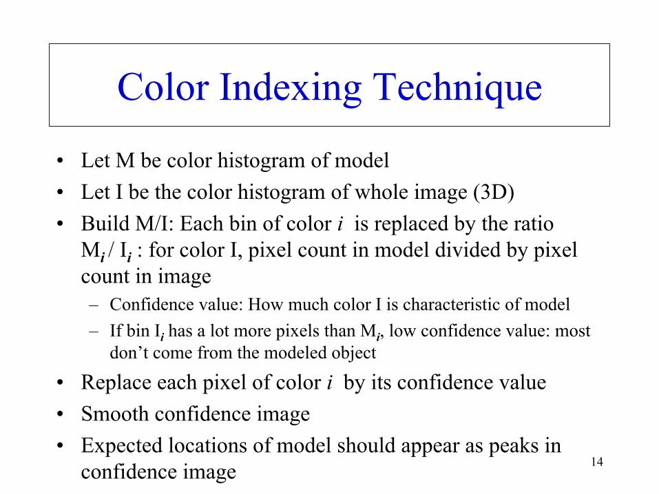
Color Indexing Technique

• Let M be color histogram of model• Let I be the color histogram of whole image (3D)• Build M/I: Each bin of color i is replaced by the ratio

Mi / Ii : for color I, pixel count in model divided by pixel count in image– Confidence value: How much color I is characteristic of model– If bin Ii has a lot more pixels than Mi, low confidence value: most

don’t come from the modeled object

• Replace each pixel of color i by its confidence value• Smooth confidence image• Expected locations of model should appear as peaks in

confidence image

15

Illustration of Color Indexing

Pixels of image that are in small numbers are favoredColor confidence M/I (3D)

Image histogram I (3D table)

Model histogram M (3D)

White Red

16

Extensions of Color Indexing

• In Color Indexing, we measure 3 color components at every pixel, then build a histogram

• We can collect a more complex feature vector at every pixel– Apply masks to measure color gradients in 2 orthogonal directions– Apply mask to measure Laplacian

• This defines components of a local feature vector

• Construct histograms of feature vector for image and model– More dimensions than color histograms

• Locate object from cluster of pixels with high confidence value as in color indexing

17

Example 2: Salient Point Method• Find most salient point of model

– For every pixel, define a high-dimensional feature vector– For every pixel, find the distance of its feature vector to all the

others.– Keep as salient point the pixel with the largest distance to the

others

• Locating a model in image: – For every image pixel, find feature vector– Calculate distance from feature vector of every pixel to salient

point of model– Select pixel with minimum distance to salient point of model as

candidate point corresponding to salient point

• This is a “focus of attention” mechanism. A more complete recognition method can be used in the region around the detected salient point.

18

Example 3: Geometric Hashing

• Uses affine projection model– Flat objects “far” from camera– Objects may be at an angle with respect to camera

optical axis

19

Special Homography: Affine Transformation

+

=

+=

z

y

x

o

o

o

www

ow

ttt

ZYX

rrrrrrrrr

ZYX

TRPP

333231

232221

131211

],,[

xw tZrYrXrX +++= 013012011

And the image coordinates of (Xw, Yw, Zw) are

z

xww tZrYrXr

tZrYrXrfZfXx++++++

==033032031

013012011/

20

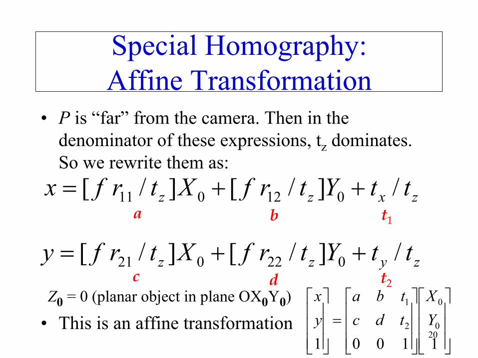
• P is “far” from the camera. Then in the denominator of these expressions, tz dominates. So we rewrite them as:

• This is an affine transformation

zxzz ttYtrfXtrfx /]/[]/[ 012011 ++=a t1b

zyzz ttYtrfXtrfy /]/[]/[ 022021 ++=c t2d

=

110010

0

2

1

YX

tdctba

yxZ0 = 0 (planar object in plane OX0Y0)

Special Homography: Affine Transformation

21

• With non projective coordinates, mapping from point M to point M’ is

• Mapping from vector M0M to M’0M’ is

•• Therefore, components a1 and a2 of a point M are

invariant in an affine transformation

Properties of Affine Transformation

TAMM' +=⇒

+

=

2

1

''

tt

yx

dcba

yx

MMAM'M' 00 =

212121 V'V'V'AVAVAVVVV 212121 aaaaaa +=⇒+=⇒+=

TAM'M 00 +=

22

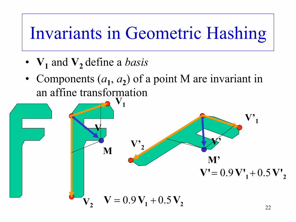
Invariants in Geometric Hashing• V1 and V2 define a basis• Components (a1, a2) of a point M are invariant in

an affine transformationV1

V2

V’2

V’1

V’V

MM’

21 V'V'V' 5.09.0 +=

21 VVV 5.09.0 +=

23

Building a Table from Models• Coordinate pairs are “signatures” or “keys” of models

– We use these invariants to detect models• For each model

– For each basis (3 points), consider each feature point, find 2 coordinates. They locate a bin in a table. Store index of model (1 or 2) in bin

M1,

M1,

M1,2

a1

a2Model 1 Model 2

• Expensive (order m4) but doneonly once for the set of models

24

Using the Table for Recognition• Pick 3 feature points from the image to define a basis.• Compute coordinate pairs of all remaining image feature points

with respect to that basis.• Use these coordinates to access bins in the table

– In a bin, we may find the index of model Mi - if the corresponding 3 points in model Mi were used as basis, and the corresponding point in the model was considered when building the table

• Repeat for all plausible triples of feature points• Keep track of scores of each model Mi encountered• Models that obtain high scores are recorded as possible detections

25

Plus and Minus of Invariants

• Plus: no storing of a set of views• Minus: no ideal set of measurements we can apply

to all objects. No universal features independent of viewing position and depending only on nature of object– What simple invariances would distinguish a fox from a

dog?

26

Parts and Structural Descriptions

• Many objects seem to contain natural parts– Face contains eyes, nose, mouth– These can be recognized on their own– Then recognition of object can use identified parts

27

Part Decomposition Assumptions

• Each object can be decomposed into a small set of generic components– Generic: all objects can be described as different

combinations of same components– Stable decomposition: decomposition is preserved

across views of object

• Parts can be classified independently from whole object

28

From Parts to Structure

• Two main approaches– Repeat decomposition process:

• Certain parts are decomposed into simpler parts– Identify low-level parts, then group them to form

higher-level parts

29

Recognition Process

• Describe objects in terms of constituent parts• Locate parts• Classify them into different types of generic

components• Check relationships between parts• Select objects for which structure matches

detected relationships best

30

Advantages• Parts are simpler to detect than whole object, vary

less with change of view• Variability of object views is due to variability of

structure, and structure can be detected by connectivity between parts– If we can recognize Tinkertoy elements, then we can

recognize objects from a catalog of structures

31

Relations between Parts

• The relations between parts are the invariants– Letter A:

• 3 line segments• 2 line segments meet at vertex

• Invariances are expressed in terms of relations between two or more parts– Above, to the left of, longer than, containing, …

32

2D and 3D Relations

– For 2D applications, distances and angles– For 3D applications, “connected together”, “larger

than”, “inside of” remain invariant over a wide range of viewing positions

– This allows to distinguish between configurations of similar parts in different arrangements

• Fundamental to human visual system• Pigeons recognize successfully people, trees,

pigeons, letters, but don’t make distinction between figure and scrambled version: recognition from local parts, not structure

33

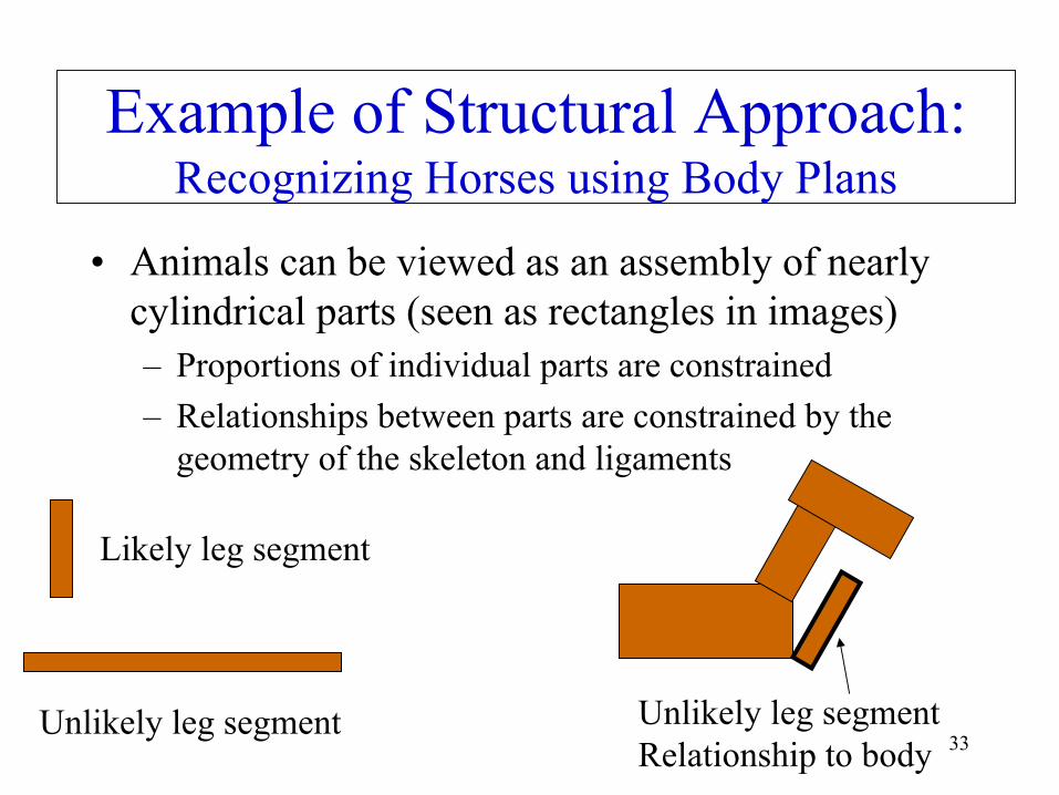
Example of Structural Approach: Recognizing Horses using Body Plans

• Animals can be viewed as an assembly of nearly cylindrical parts (seen as rectangles in images)– Proportions of individual parts are constrained– Relationships between parts are constrained by the

geometry of the skeleton and ligaments

Likely leg segment

Unlikely leg segment Unlikely leg segmentRelationship to body

34

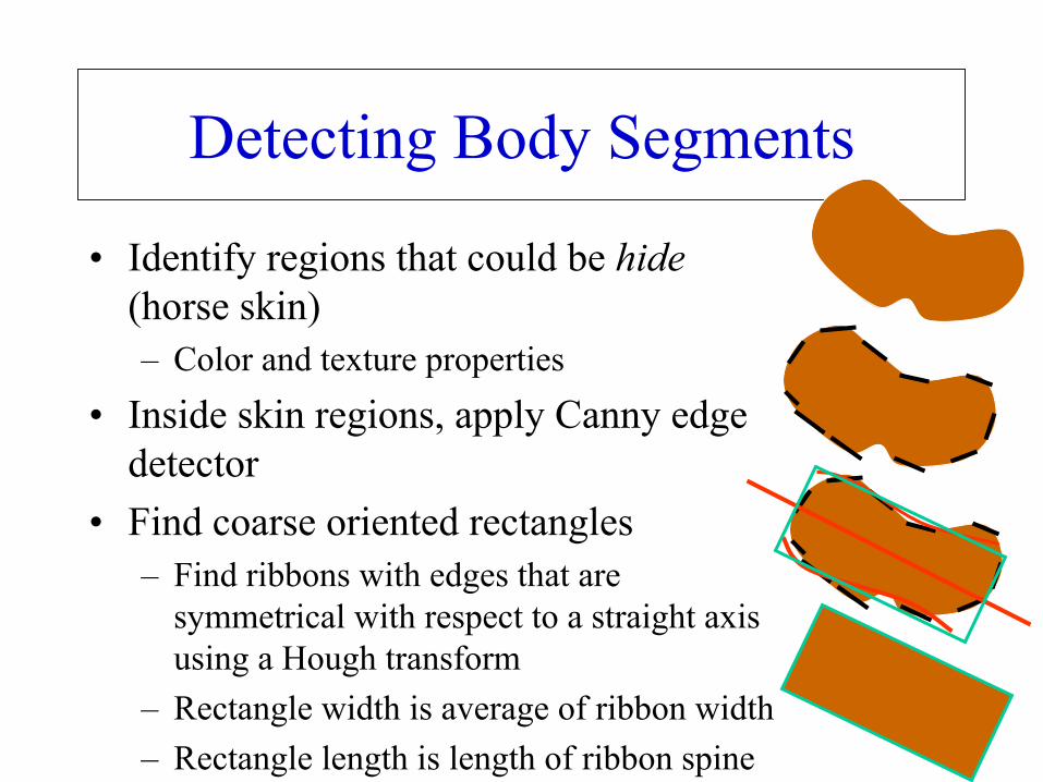
Detecting Body Segments

• Identify regions that could be hide(horse skin)– Color and texture properties

• Inside skin regions, apply Canny edge detector

• Find coarse oriented rectangles– Find ribbons with edges that are

symmetrical with respect to a straight axis using a Hough transform

– Rectangle width is average of ribbon width– Rectangle length is length of ribbon spine

35

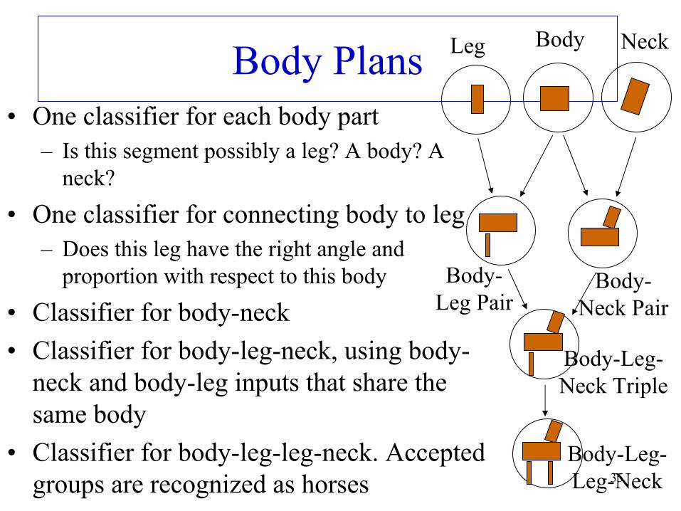
Body Plans• One classifier for each body part

– Is this segment possibly a leg? A body? A neck?

• One classifier for connecting body to leg– Does this leg have the right angle and

proportion with respect to this body

• Classifier for body-neck• Classifier for body-leg-neck, using body-

neck and body-leg inputs that share the same body

• Classifier for body-leg-leg-neck. Accepted groups are recognized as horses

Leg Body Neck

Body-Leg Pair

Body-Neck Pair

Body-Leg-Neck Triple

Body-Leg-Leg-Neck

36

Classifier Training

• Body segments are defined by a vector with components – Centroid x and y, rectangle width and height, angle

• classifiers that use these features and decide if something is a horse or not are used – SVM classifiers

• Training images from CD “Arabian horses” of Corel photo library

37

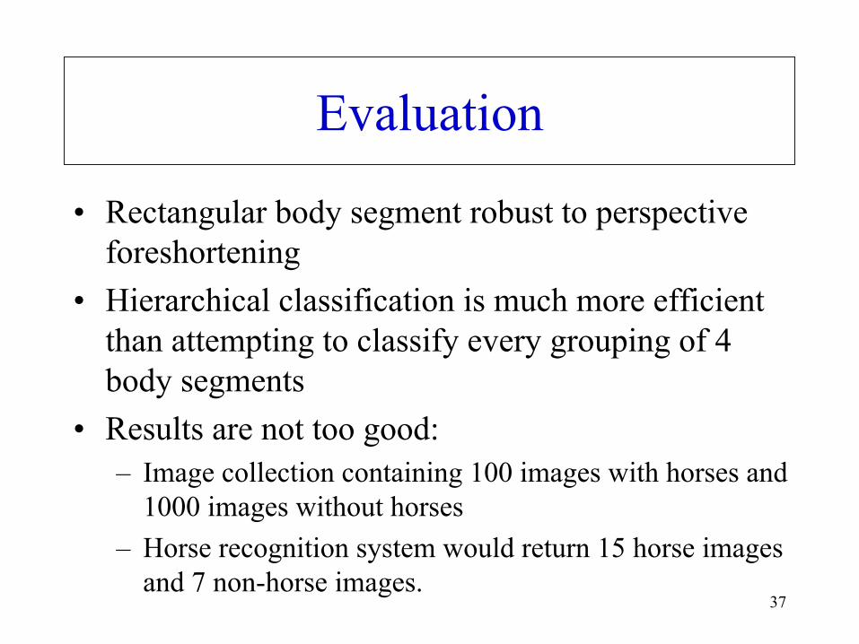
Evaluation

• Rectangular body segment robust to perspective foreshortening

• Hierarchical classification is much more efficient than attempting to classify every grouping of 4 body segments

• Results are not too good: – Image collection containing 100 images with horses and

1000 images without horses– Horse recognition system would return 15 horse images

and 7 non-horse images.

38

Experiments

39

Problems with Part Decomposition

• Decomposition falls sort of characterizing object specifically enough– Dog and cat have similar parts– Differentiation is possible if we check detailed shape at

particular locations (such as the snout)

40

Other Problems

• Many objects do not decompose naturally into a union of clearly distinct parts– What is a decomposition of a shoe

• Finding parts such as limbs, torso reliably is very difficult

• Useful, but insufficient

41

Which Approach is Best?

• Invariants, parts description, alignment?• No single best scheme is appropriate for all cases• Recognition system must exploit the regularities

of given domain• In humans, several agents using different

techniques work in parallel. If one agent succeeds, we are not aware of those that failed

42

References

• High Level Vision: Object Recognition and Visual Cognition, Shimon Ullman, MIT Press, 1996.

• M.J. Swain and D.H. Ballard. Indexing via Color Histogram. Proc. ICCV, pp. 390-393, 1990.

• F. Ennesser and G. Medioni. Finding Waldo, or Focus of Attention using Local Color Information. PAMI 17, 8, 1995.

• M.J. Swain, C.H. Frankel and M. Lu. View-Based Techniques for Searching for Objects and Textures (Salient Points). http://people.cs.uchicago.edu/~swain/pubs

• D.A. Forsyth and M.M. Fleck. Body Plans. Proc. CVPR 1997.http://www.cs.berkeley.edu/~daf/book3chaps.html