Object Detection based on Convolutional Neural Network

Shijian TangDepartment of Electrical Engineering

Stanford Universitysjtang@stanford.edu

Ye YuanDepartment of Computer Science

Stanford Universityyy0222@cs.stanford.edu

Abstract

In this paper, we develop a new approach for detectingmultiple objects from images based on convolutional neuralnetworks (CNNs). In our model, we first adopt the edge boxalgorithm to generate region proposals from edge maps foreach image, and perform forward passing of all the propos-als through a fine-tuned CaffeNet model. Then we get theCNNs score for each proposal by extracting the output ofsoftmax which is the last layer of CNN. Next, the proposalsare merged for each class independently by the greedy non-maximum suppression (NMS) algorithm. At last, we evalu-ate the mean average precision (mAP) for each class. ThemAP of our model on PASCAL 2007 test dataset is 37.38%.We also discuss how to further improve the performancebased on our model in this paper.

1. IntroductionConvolutional neural networks (CNNs) has been widely

used in visual recognition from 2012 [1] due to its high ca-pability in correctly classifying images. In [1], the authorsshow an extremely improvement on the accuracy of imageclassification in ImageNet Large Scale Visual RecognitionChallenge (ILSVRC). And CNNs become the most prefer-able choice for solving image classification challenges. Be-sides image classification, researchers have extend the ap-plication of CNNs to several other tasks in visual recogni-tion such as localization [2], segmentation [3], generatingsentences from image [4], as well as object detection [5].

In our project, we mainly focus on the task of object de-tection which has tremendous application in our daily life.The goal of object detection is recognise multiple objects ina single image, not only to return the confidence of the classfor each object, but also predict the corresponding boundingboxes.

Among most of the works in object detection, regionCNNs (rCNN) [5] is the most remarkable one that combinesselective search [6], CNNs, support vector machines (SVM)and bounding box regression together to provide a high per-

formance in object detection.In this paper, we will provide an alternative approach of

object detection by reducing the complexity of the rCNN.First, we adopt edge box [7], a recent published algorithm togenerate region proposals, instead of selective search usedin rCNN. [8] shows that even though the mean average pre-cision (mAP) between edge boxes and selective search arealmost the same, edge boxes runs much faster than selectivesearch. Secondly, we remove all of the class specific SVMs,and directly use the output of softmax in the last layer ofCNN as our score. To compensate the possible performancedegrade raised by removing SVMs, we carefully design ourtraining data to fine-tune CNN. Fig. 1 is an overview of ourmodel.

Figure 1: The overview of our object detection system. 1).Edge box algorithm generates proposals. 2). A fine-tunedCNN with object classes plus one background class to ex-tract the CNN features for each proposal. 3) Employ thesoftmax to give the confidence (score) of all the classes foreach proposal (which is typically the last layer of CNN).4). For each class, independently use the non-maximumsuppression (NMS) to greedily merge the overlapped pro-posals.

In addition to the previous model, we also develop a tra-ditional model as our baseline. In this model, we adopt slid-ing window to generate proposals, and use histogram orien-tation gradient (HOG) features to describe such proposals.Then we use our trained linear SVM to score each proposal.

The rest of this paper can be organized as follows. Insection 2, we briefly summarize the previous work in ob-ject detection and introduce the state-of-art approaches. Insection 3, we will cover more details of the technical ap-proaches in our model including the general framework,theoretical background as well as performance evaluation

1

metrics. In section 4, we will present our experiment resultsand briefly discuss the results. Section 5 will conclude ourwork and discuss the method to further improve the perfor-mance of our model.

2. Background

Object detection becomes an attractive topic in visualrecognition area in the last decade. In the early stage, peopletend to design features from raw images to improve the per-formance of the detection. Among these features, SIFT [9]and HOG [10] features are the most successful ones. Thesefeatures combined with SVMs have successfully detect thepedestrians from images. However, when these models areapplied into multiple classes and object detection in a singleimage, the performance is not as our expected.

Instead of using linear SVMs, some other works try touse ensemble SVMs [11] as well as latent SVMs [12] basedon HOG feature description. But the performance of objectdetection still barely improves.

People switch to focus on CNNs since [1] shows a signif-icant improvement of classification accuracy by employinga deep CNNs. Unlike classification, the detection task alsorequires us to localize the object by specifying a bound-ing edge box. Therefore, we can not directly use CNNsin object detection without solving the localization prob-lem. [2] tries to treat the localization problem as a regres-sion task. But the performance has minimal improvement.Then other researchers [13] adopt the sliding window com-bined with CNNs as one possible solution. However, dueto the exhaustive nature of sliding window with high com-putational complexity, this method can not be practicallyimplemented. Even though sliding window approach cannot work in practice, this method provides an idea that issolving localization by classifying region proposals of theimages.

Instead of sliding window, several algorithms are alsocapable to generate proposals efficiently, such as objectness[14], selective search [6], category-independent object pro-posals [15], constrained parametric min-cuts (CPMC) [16]and edge [7]. In the rCNN paper [5], the authors chooseselective search as proposal generation algorithm due to itsfast computational time. In this paper, we will choose a newpublished algorithm named edge instead of selective searchfor object detection.

Other people also develop weakly supervised learning[17] and deformable CNNs [18] to detect objects last year.

3. Approach

In this section, we will cover the details of our objectdetection model.

3.1. Proposal generation

In this paper we will use the edge boxes as our proposalgeneration algorithm. The basic idea of edge boxes is thatthis algorithm generates and scores the proposal based onthe edge map of the image. Specifically, in the first step weshould generate an edge map with a structured edge detec-tor where each pixel contains a magnitude and orientationinformation of the edge.

Then we group the edges together by a greedy algorithmwhere the sum of orientation of all the edges in the groupis less than pi/2. After that, we will compute the affinitybetween two edge groups which is important for the scorecomputation.

Next, for a given bounding box, we will compute thescore of the bounding box based on the edge groups entirelyinside the box.

At last, we use the non-maximal suppression to mergethe bounding box to get the proposals.

Compared with the selective search which has been cho-sen in the rCNN, [8] shows that for VOC 2007 dataset, themAP of edge boxes is 31.8% which is slightly larger thanselective search with mAP as 31.7%. One advantage ofedge boxes is that the runtime is much faster than the ma-jority of the proposal generation schemes. For edge boxes,the average runtime is 0.3 seconds while for selective searchas 10 seconds.Therefore, the edge boxes decreases the timecomplexity without degrading the performance. Hence, wechoose the edge boxes as the proposal generation algorithm.

3.2. Training procedure

In this paragraph, we will describe preparing our trainingdata and fine-tuning caffe model. As we mentioned in sec-tion 1, for compensating the removal SVMs from the rCNN,we will carefully design our training data, especially for thebackground data.

In the rCNN model, the authors train both CNN and classspecific SVMs using different training data set. For CNN,they choose the bounding box with IoU (intersection overunion) larger than 0.5 as positive data, others as negative(background) data. For SVMs, they use the ground-truthas positive data to improve localization precision, IoU lessthan 0.3 as negative data and ignore all the rest of cases.

In our approach, all the training data are extracted fromthe raw images. As we eliminate the SVMs, we did notchoose IoU as 0.5 to split positive and negative (also knownas background) data for CNN, because that would decreasethe performance of localization. Our schemes are as fol-lows. For the detection problem, during the test time, thenumber of background proposals is typically much largerthan that of the positive proposals. Hence, intuitively, weneed more background data compared with positive data fortraining. So, we collect background data four times largerthan the positive data. Note that we will not add more back-

2

ground data, since it will make the training dataset imbal-ance and, therefore, harder for a classifier to classify it.

Then we divide the background data into four folders1,2,3,4. For folder 1, the IoU with ground truth are be-tween 0.5 and 0.7, for folder 2, the IoU with ground truthare between 0.3 and 0.5, for folders 3 and 4, the IoU withground truth are less than 0.3. In the case of positive data,we randomly extract a region from raw image, if the IoUwith ground truth is larger than 0.7, it is a positive data withthe same class label as the ground truth. The last step isshuffling all the data. By designing the training data in thisway, we can suffer a precise localization without class spe-cific SVMs.

The next step is fine-tuning the pre-trained CNN mod-els using the generated training data as we described above.We choose the CaffeNet model as our pre-trained model.This model is a replicate of AlexNet, having 5 convolu-tional layers and pre-trained on the ILSVRC2012 dataset.We change the output number of last layers to 21 (for VOC2007 dataset, 20 object classes plus 1 background class).We will describe the process and results for tuning the Caf-feNet model.

3.3. Testing procedure

In the testing time, we firstly generate regional propos-als by edge boxes, and then perform the forward pass forall of the proposals through the fine-tuned CNN. Note thatsince the input size of CaffeNet model is fixed as 227× 227pixels, the proposals with different shapes are resized to therequired shape before forward pass.

After that, we will extract the output of the softmax as a21-element vector for each proposal, with each entry in thevector represent the confidence of the corresponding pro-posal in each class.

The we employ the non-maximum suppression (NMS)algorithm to ignore the redundant proposals. The basic ideaof this algorithm is that sort the proposals by the confidence(also known as score), and then ignore the proposals over-laping with a higher-scored proposal. The threshold of theoverlap is typically defined as the IoU between two propos-als. Note that the IoU threshold will affect the performanceof our detector, which should be tuned carefully to achievethe best performance.

To evaluate the performance of the detection, we use themean average precision (mAP). The mAP equals to the in-tegral over the precision-recall curve p(r).

mAP =

∫ 1

0

p(r)dr (1)

To determine the precision-recall curve, we need to com-pute the true positive and false positive value of our predic-tion first. We use the IoU (intersection of union) to deter-

mine the successful detection by

IoU =Apred

⋂Agt

Apred

⋃Agt

(2)

where Apred and Agt are the areas included in the predictedand ground truth bounding box, respectively. Then we des-ignate a threshold for IoU, for example 0.5, if the IoU ex-ceeds the threshold, the detection marked as correct detec-tion. Multiple detections of the same object are consideredas one correct detection and with others as false detections.After we get the true positive and false positive values, wecan compute the precise-recall curve, and then evaluate themAP. Details about the error analysis can be found in [19].

3.4. Baseline model

As the baseline, one approach of generating proposal weexperimented is using features. [10]The process of localiza-tion and classification are separated. Firstly, HOG features,a binary-classification SVM and Non-Maximum Suppres-sion are used for localisation, and then result boxes fromthe previous process will be classified by CNN.

When in the training process of the SVM, comparablenumbers of object and background boxes are used. HOGfeatures of such boxes are passed into the SVM to train theweights. SVM will determine if one box contains objects oronly background.

In the testing process. HOGs of sliding windows ofthrees shapes and three scales are passed into the trainedSVM to obtain scores on each label. Then, NMS is used totake away bounding boxes that overlap others with higherscores. The proposals remained after this process will be thelocalization of the objects. These region will then passedinto the CNN for classification. The mAP we obtainedbased on this model is 22.6%.

For more detail of this model, please have a look as ourCS 231A final project report.

4. Experiment Results4.1. Dataset description

We adopt the VOC 2007 dataset in our project, which isa popular dataset for classification, detection and segmenta-tion [20]. This dataset contains 5011 images for the task ofdetection and classification. All the images are divided intotraining set and validation set. For the training dataset wehave 2501 images, and 2510 images for validation.

The objects in the dataset can be classified into 20classes. Each image contains more than one object whichare not necessarily in the same class. The total number ofobjects in this dataset is 12608, with 6301 in training datasetand 6307 in validation dataset. On the average, there will be2.51 objects per image. Therefore, this dataset is an appro-priate choice for detection problem. In addition, the objects

3

can be also described by the regular objects and difficult ob-jects. The difficult objects are typically not clearly visiblesuch as occluded by other objects. These objects marked asdifficulty can not be simply classified or detected withoutadditional information such as the view of the image. Thisis beyond the topic of this project. Therefore, in our projectwe ignore the difficult objects as most other works did.

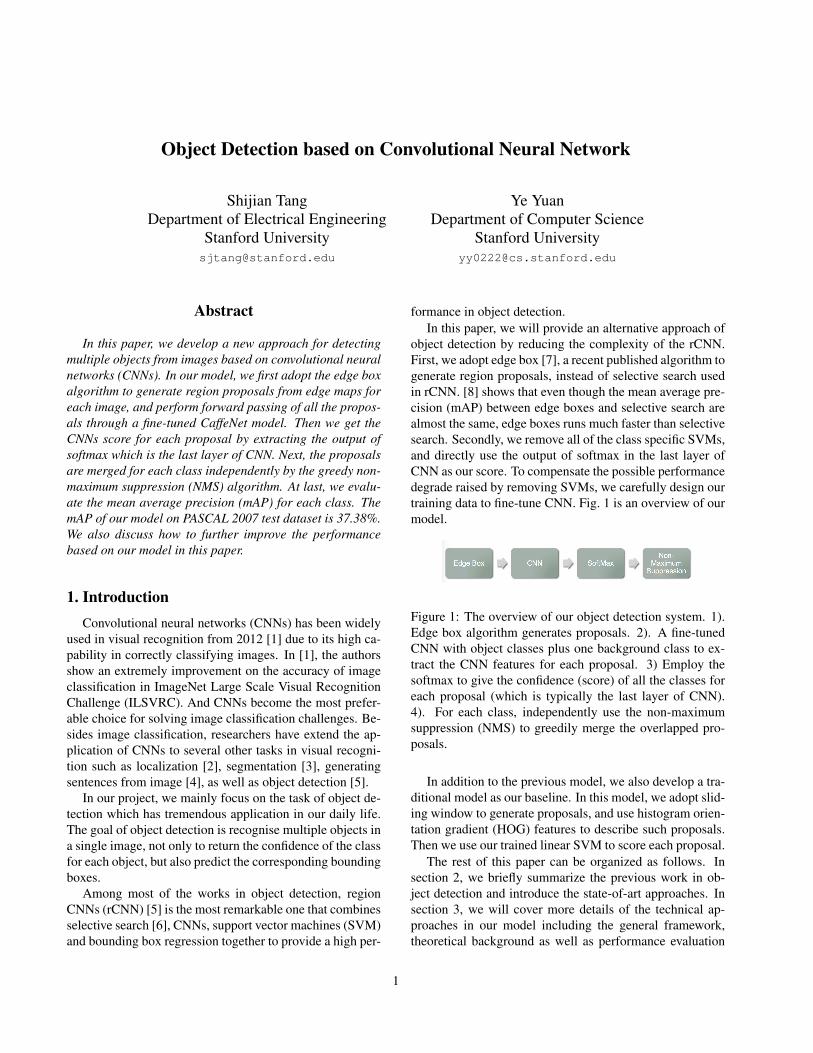
As we mentioned in the previous section, we have pre-processed the training data as well as validation data forfine-tuning CNN. We have generated 30120 training datawith 6024 positive images labeled by 20 classes, and 24096background images. Also, we get 30232 validation datawith 6064 positive images and 24168 background images.Fig. 2 illustrates the samples of resized training data withpositive and negative labels.

For the test data, the VOC 2007 has released the wholetest dataset with 4952 images and the corresponding groundtruth bounding box for each object. There is no object la-beled as ”difficult” in the test dataset.

(c) (d)

Figure 2: The samples from training data with all imagesresized into 256×256 pixels. The first two rows are positiveimage, and the second two rows are negative images.

4.2. Fine-tuning Caffe

The goal of the training process is to fine-tune the pre-trained CaffeNet model on our dataset. Our strategy is that

first we have frozen all the layers except for the last layer(softmax layer), then use a relatively aggressive learningrate to train the last layer from scratch. This procedure isequivalent to use the 4096 dimension CNN features to traina softmax classifier. We initialize the learning rate as 0.001and decrease the learning rate by a factor of 0.9 after every2000 iterations. After the 10000 iterations, the validationaccuracy is 0.780875, with loss as 0.758219.

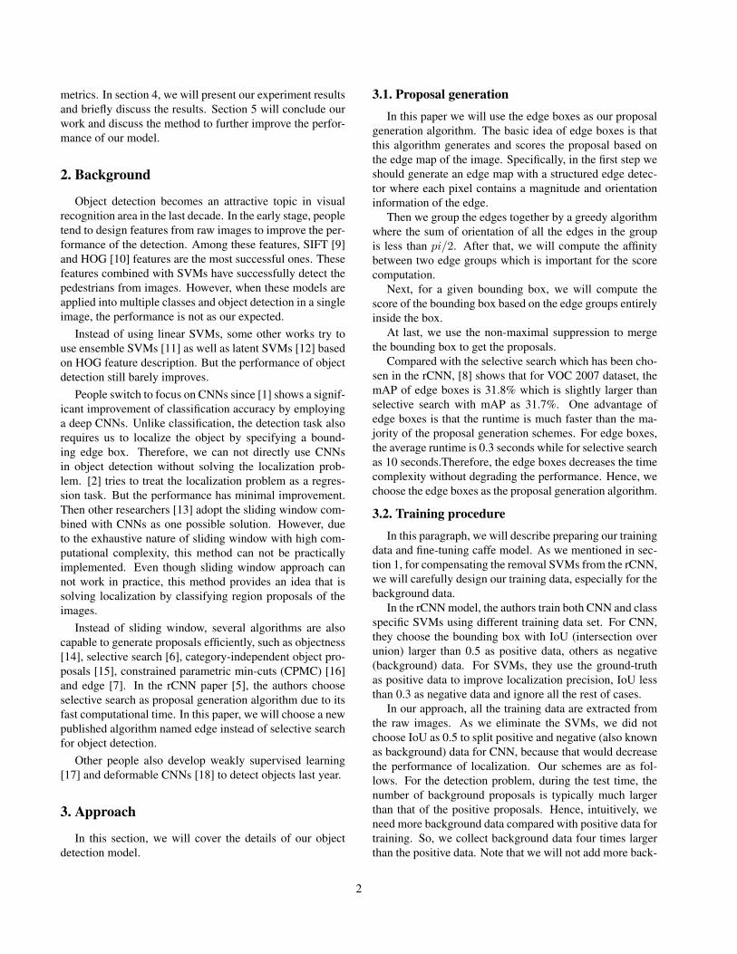
Then for the next step of fine tuning, we release all thelayers, and train them together. Here, we choose a rela-tively small learning rate initialized as 5e-6, and decreasethe learning rate by a factor of 0.9 after every 2000 itera-tions. After 30000 (40000 in total) iterations, we can getthe the validation accuracy as 89%. And the loss is 0.4474,as Fig. 3 shows.

Figure 3: The accuracy and loss for the fine-tuned CaffeNetfor VOC 2007 object detection task.

4.3. Testing results

In the testing procedure, we first generate proposals foreach test image by edge boxes. The average run time foreach image is around 0.3 seconds. However, for each imagethe number of proposals ranges from 2000 up to 6000. Weuse the terminal GPU+Caffe instance, the forward pass foreach proposal takes roughly 54 ms per proposal and around1.8 to 5.4 minutes per image (including the time of loadand save files). Based on the analysis above, we can con-clude that for the worst case the total runtime for pass allthe test images is roughly 445.68 hours. Hence, for thiscourse project, we need to reduce the number of proposalsper image heuristically.

We find that VOC 2007 test dataset, most of the objectsare large. Therefore, we can remove the proposals with tinyarea which is generally impossible to be good candidates

4

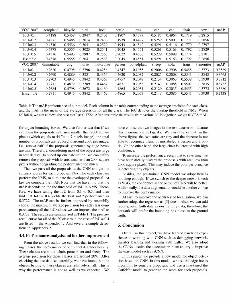
VOC 2007 aeroplane bicycle bird boat bottle bus car cat chair cow mAPIoU=0.1 0.4188 0.5458 0.2947 0.2402 0.1807 0.4377 0.5187 0.4964 0.1719 0.2815IoU=0.2 0.4271 0.5485 0.3014 0.2436 0.1939 0.4427 0.5259 0.5007 0.1771 0.2856IoU=0.3 0.4340 0.5536 0.3041 0.2529 0.1943 0.4542 0.5291 0.5116 0.1779 0.2797IoU=0.4 0.4378 0.5555 0.3023 0.2541 0.2045 0.4551 0.5261 0.5163 0.1792 0.2829IoU=0.5 0.4316 0.5493 0.2987 0.2563 0.2022 0.4506 0.5229 0.5098 0.1774 0.2701Esemble 0.4378 0.5555 0.3041 0.2563 0.2045 0.4551 0.5291 0.5163 0.1792 0.2856

VOC 2007 diningtable dog horse motorbike person pottedplant sheep sofa train tvmonitor mAPIoU=0.1 0.2620 0.4795 0.3796 0.4258 0.4347 0.1955 0.2006 0.2908 0.5455 0.3773 0.3589IoU=0.2 0.2690 0.4889 0.3831 0.4364 0.4620 0.2032 0.2025 0.3008 0.5541 0.3843 0.3665IoU=0.3 0.2703 0.4945 0.3842 0.4368 0.4757 0.2048 0.2134 0.3063 0.5538 0.3930 0.3712IoU=0.4 0.2711 0.4872 0.3789 0.4467 0.4831 0.2053 0.2143 0.3085 0.5507 0.3835 0.3722IoU=0.5 0.2684 0.4798 0.3672 0.4460 0.4865 0.2031 0.2129 0.3035 0.5455 0.3775 0.3680

Ensemble 0.2711 0.4945 0.3842 0.4467 0.4865 0.2053 0.2143 0.3085 0.5541 0.3930 0.3738

Table 1: The mAP performance of our model. Each column in the table corresponding to the average precision for each class,and the mAP is the mean of the average precision for all the class. The IoU denotes the overlap threshold in NMS. WhenIoU=0.4, we can achieve the best mAP as 0.3722. After ensemble the results from various IoUs together, we get 0.3738 mAP.

for object bounding boxes. We also further test that if wecut down the proposals with area smaller than 2000 squarepixels (which equals to 44.7×44.7 pixels image), the totalnumber of proposals are reduced to around 2000 per image,i.e., almost half of the proposals generated by edge boxesare tiny. Therefore, considering most of the object are largein test dataset, to speed up our calculation, we can safelyremove the proposals with its area smaller than 2000 squarepixels without degrading the performance too much.

Then we pass all the proposals to the CNN and get thesoftmax scores for each proposal. Next, for each class, weperform the NMS, to eliminate the overlapped proposal. Atlast we compute the mAP. Note that we have find that themAP depends on the the threshold of IoU in NMS. There-fore, we have tuning the IoU from 0.1 to 0.5, and thenfind that IoU = 0.4 yields the best mAP performance as0.3722. The mAP can be further improved by ensembllychoose the maximum average precision for each class com-pared among all the IoU values, we can improve the mAP to0.3738. The results are summarized in Table 1. The precise-recall curve for all of the 20 classes in the case of IoU = 0.4are listed in the Appendix 1. And several example detec-tions in Appdendix 2.

4.4. Performance analysis and further improvement

From the above results, we can find that in the follow-ing classes, the performance of our model degrades heavily.These classes are bottle, chair, pottedplant and sheep. Theaverage precision for those classes are around 20%. Afterchecking the test data set carefully, we have found that theobjects belong to these classes are relatively small. This iswhy the performance is not as well as we expected. We

have choose the two images in the test dataset to illustratethis phenomenon in Fig. 4a. We can observe that, in theabove figure, the two sofas are tiny and the detector is notable to recognize them. It mislabeled a person and a bot-tle. On the other hand, the large chair is detected with highconfidence.

To increase the performance, recall that to save time, wehave heuristically discard the proposals with area less than2000 square pixels. This may induce the poor performancein detecting tiny objects.

Besides, the pre-trained CNN model we adopt here isnot deep enough. If we switch to the deeper network suchas VGG, the confidence as the output of CNN will be better.Additionally, the data augmentation could be another choiceto improve the performance.

At last, to improve the accuracy of localization, we canfurther adopt the regressor as [5] does. Also, we can addmore ground truth data as our training data, therefore, thenetwork will prefer the bounding box close to the groundtruth.

5. Conclusion

Overall in this project, we have learned hands on expe-rience in working with CNN such as debugging network,transfer learning and working with Caffe. We also adoptthe CNNs to solve the detection problem and try to improvethe exist model such as rCNN.

In this paper, we provide a new model for object detec-tion based on CNN. In this model, we use the edge boxesalgorithm to generate proposals, and use a fine-tuned theCaffeNet model to generate the score for each proposals.

5

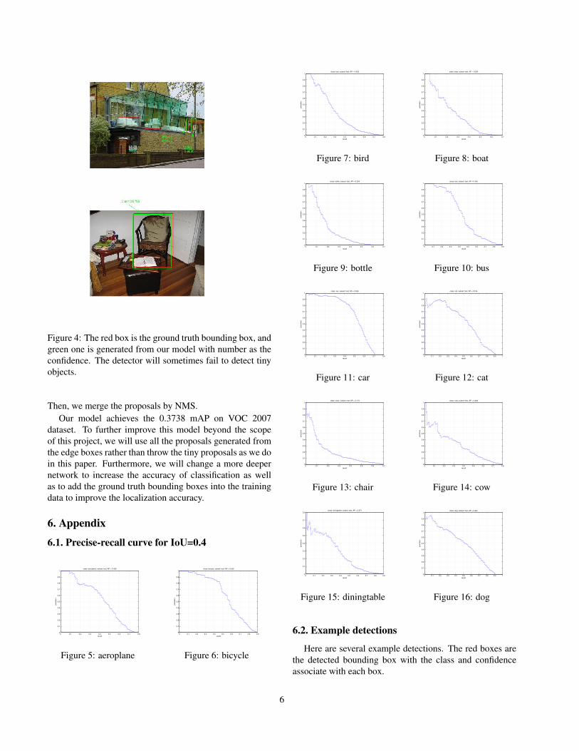
Figure 4: The red box is the ground truth bounding box, andgreen one is generated from our model with number as theconfidence. The detector will sometimes fail to detect tinyobjects.

Then, we merge the proposals by NMS.Our model achieves the 0.3738 mAP on VOC 2007

dataset. To further improve this model beyond the scopeof this project, we will use all the proposals generated fromthe edge boxes rather than throw the tiny proposals as we doin this paper. Furthermore, we will change a more deepernetwork to increase the accuracy of classification as wellas to add the ground truth bounding boxes into the trainingdata to improve the localization accuracy.

6. Appendix

6.1. Precise-recall curve for IoU=0.4

0 0.1 0.2 0.3 0.4 0.5 0.6 0.7 0.80

0.1

0.2

0.3

0.4

0.5

0.6

0.7

0.8

0.9

1

recall

pre

cis

ion

class: aeroplane, subset: test, AP = 0.438

Figure 5: aeroplane

0 0.1 0.2 0.3 0.4 0.5 0.6 0.7 0.8 0.90

0.1

0.2

0.3

0.4

0.5

0.6

0.7

0.8

0.9

1

recall

pre

cis

ion

class: bicycle, subset: test, AP = 0.556

Figure 6: bicycle

0 0.1 0.2 0.3 0.4 0.5 0.6 0.7 0.80

0.1

0.2

0.3

0.4

0.5

0.6

0.7

0.8

0.9

1

recall

pre

cis

ion

class: bird, subset: test, AP = 0.302

Figure 7: bird

0 0.1 0.2 0.3 0.4 0.5 0.6 0.70

0.1

0.2

0.3

0.4

0.5

0.6

0.7

0.8

0.9

1

recall

pre

cis

ion

class: boat, subset: test, AP = 0.254

Figure 8: boat

0 0.1 0.2 0.3 0.4 0.5 0.6 0.70

0.1

0.2

0.3

0.4

0.5

0.6

0.7

0.8

0.9

1

recall

pre

cis

ion

class: bottle, subset: test, AP = 0.204

Figure 9: bottle

0 0.1 0.2 0.3 0.4 0.5 0.6 0.7 0.8 0.90

0.1

0.2

0.3

0.4

0.5

0.6

0.7

0.8

0.9

1

recall

pre

cis

ion

class: bus, subset: test, AP = 0.455

Figure 10: bus

0 0.1 0.2 0.3 0.4 0.5 0.6 0.7 0.80

0.1

0.2

0.3

0.4

0.5

0.6

0.7

0.8

0.9

1

recall

pre

cis

ion

class: car, subset: test, AP = 0.526

Figure 11: car

0 0.1 0.2 0.3 0.4 0.5 0.6 0.7 0.8 0.9 10

0.1

0.2

0.3

0.4

0.5

0.6

0.7

0.8

0.9

1

recall

pre

cis

ion

class: cat, subset: test, AP = 0.516

Figure 12: cat

0 0.1 0.2 0.3 0.4 0.5 0.6 0.70

0.1

0.2

0.3

0.4

0.5

0.6

0.7

0.8

0.9

1

recall

pre

cis

ion

class: chair, subset: test, AP = 0.179

Figure 13: chair

0 0.1 0.2 0.3 0.4 0.5 0.6 0.7 0.80

0.1

0.2

0.3

0.4

0.5

0.6

0.7

0.8

0.9

1

recall

pre

cis

ion

class: cow, subset: test, AP = 0.283

Figure 14: cow

0 0.1 0.2 0.3 0.4 0.5 0.6 0.7 0.8 0.90

0.1

0.2

0.3

0.4

0.5

0.6

0.7

0.8

recall

pre

cis

ion

class: diningtable, subset: test, AP = 0.271

Figure 15: diningtable

0 0.1 0.2 0.3 0.4 0.5 0.6 0.7 0.8 0.9 10

0.1

0.2

0.3

0.4

0.5

0.6

0.7

0.8

0.9

1

recall

pre

cis

ion

class: dog, subset: test, AP = 0.487

Figure 16: dog

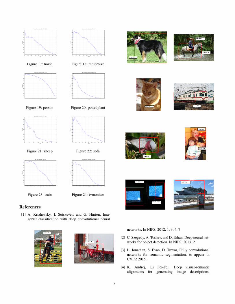
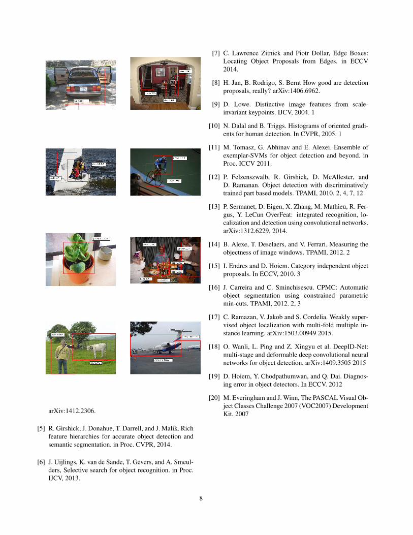
6.2. Example detections

Here are several example detections. The red boxes arethe detected bounding box with the class and confidenceassociate with each box.

6

0 0.1 0.2 0.3 0.4 0.5 0.6 0.7 0.8 0.90

0.1

0.2

0.3

0.4

0.5

0.6

0.7

0.8

0.9

1

recall

pre

cis

ion

class: horse, subset: test, AP = 0.379

Figure 17: horse

0 0.1 0.2 0.3 0.4 0.5 0.6 0.7 0.8 0.90

0.1

0.2

0.3

0.4

0.5

0.6

0.7

0.8

0.9

1

recall

pre

cis

ion

class: motorbike, subset: test, AP = 0.447

Figure 18: motorbike

0 0.1 0.2 0.3 0.4 0.5 0.6 0.70

0.1

0.2

0.3

0.4

0.5

0.6

0.7

0.8

0.9

1

recall

pre

cis

ion

class: person, subset: test, AP = 0.483

Figure 19: person

0 0.1 0.2 0.3 0.4 0.5 0.6 0.70

0.1

0.2

0.3

0.4

0.5

0.6

0.7

0.8

0.9

1

recall

pre

cis

ion

class: pottedplant, subset: test, AP = 0.205

Figure 20: pottedplant

0 0.1 0.2 0.3 0.4 0.5 0.6 0.70

0.1

0.2

0.3

0.4

0.5

0.6

0.7

0.8

0.9

1

recall

pre

cis

ion

class: sheep, subset: test, AP = 0.214

Figure 21: sheep

0 0.1 0.2 0.3 0.4 0.5 0.6 0.7 0.8 0.9 10

0.1

0.2

0.3

0.4

0.5

0.6

0.7

0.8

recall

pre

cis

ion

class: sofa, subset: test, AP = 0.308

Figure 22: sofa

0 0.1 0.2 0.3 0.4 0.5 0.6 0.7 0.8 0.9 10

0.1

0.2

0.3

0.4

0.5

0.6

0.7

0.8

0.9

1

recall

pre

cis

ion

class: train, subset: test, AP = 0.551

Figure 23: train

0 0.1 0.2 0.3 0.4 0.5 0.6 0.7 0.8 0.90

0.1

0.2

0.3

0.4

0.5

0.6

0.7

0.8

0.9

1

recall

pre

cis

ion

class: tvmonitor, subset: test, AP = 0.384

Figure 24: tvmonitor

References[1] A. Krizhevsky, I. Sutskever, and G. Hinton. Ima-

geNet classification with deep convolutional neural

person 0.889

horse 0.146

networks. In NIPS, 2012. 1, 3, 4, 7

[2] C. Szegedy, A. Toshev, and D. Erhan. Deep neural net-works for object detection. In NIPS, 2013. 2

[3] L. Jonathan, S. Evan, D. Trevor, Fully convolutionalnetworks for semantic segmentation, to appear inCVPR 2015.

[4] K. Andrej, Li Fei-Fei, Deep visual-semanticalignments for generating image descriptions.

7

arXiv:1412.2306.

[5] R. Girshick, J. Donahue, T. Darrell, and J. Malik. Richfeature hierarchies for accurate object detection andsemantic segmentation. in Proc. CVPR, 2014.

[6] J. Uijlings, K. van de Sande, T. Gevers, and A. Smeul-ders, Selective search for object recognition. in Proc.IJCV, 2013.

[7] C. Lawrence Zitnick and Piotr Dollar, Edge Boxes:Locating Object Proposals from Edges. in ECCV2014.

[8] H. Jan, B. Rodrigo, S. Bernt How good are detectionproposals, really? arXiv:1406.6962.

[9] D. Lowe. Distinctive image features from scale-invariant keypoints. IJCV, 2004. 1

[10] N. Dalal and B. Triggs. Histograms of oriented gradi-ents for human detection. In CVPR, 2005. 1

[11] M. Tomasz, G. Abhinav and E. Alexei. Ensemble ofexemplar-SVMs for object detection and beyond. inProc. ICCV 2011.

[12] P. Felzenszwalb, R. Girshick, D. McAllester, andD. Ramanan. Object detection with discriminativelytrained part based models. TPAMI, 2010. 2, 4, 7, 12

[13] P. Sermanet, D. Eigen, X. Zhang, M. Mathieu, R. Fer-gus, Y. LeCun OverFeat: integrated recognition, lo-calization and detection using convolutional networks.arXiv:1312.6229, 2014.

[14] B. Alexe, T. Deselaers, and V. Ferrari. Measuring theobjectness of image windows. TPAMI, 2012. 2

[15] I. Endres and D. Hoiem. Category independent objectproposals. In ECCV, 2010. 3

[16] J. Carreira and C. Sminchisescu. CPMC: Automaticobject segmentation using constrained parametricmin-cuts. TPAMI, 2012. 2, 3

[17] C. Ramazan, V. Jakob and S. Cordelia. Weakly super-vised object localization with multi-fold multiple in-stance learning. arXiv:1503.00949 2015.

[18] O. Wanli, L. Ping and Z. Xingyu et al. DeepID-Net:multi-stage and deformable deep convolutional neuralnetworks for object detection. arXiv:1409.3505 2015

[19] D. Hoiem, Y. Chodpathumwan, and Q. Dai. Diagnos-ing error in object detectors. In ECCV. 2012

[20] M. Everingham and J. Winn, The PASCAL Visual Ob-ject Classes Challenge 2007 (VOC2007) DevelopmentKit. 2007

8