Oberwolfach Preprints - MFO · Oberwolfach Preprints (OWP) Starting in 2007, the MFO publishes a...

Oberwolfach Preprints

Mathematisches Forschungsinstitut Oberwolfach gGmbH Oberwolfach Preprints (OWP) ISSN 1864-7596

OWP 2016 - 13 RICHARD M. ARON, JAVIER FALCÓ, DOMINGO GARCÍA AND MANUEL MAESTRE Analytic Structure in Fibers

Oberwolfach Preprints (OWP) Starting in 2007, the MFO publishes a preprint series which mainly contains research results related to a longer stay in Oberwolfach. In particular, this concerns the Research in Pairs-Programme (RiP) and the Oberwolfach-Leibniz-Fellows (OWLF), but this can also include an Oberwolfach Lecture, for example. A preprint can have a size from 1 - 200 pages, and the MFO will publish it on its website as well as by hard copy. Every RiP group or Oberwolfach-Leibniz-Fellow may receive on request 30 free hard copies (DIN A4, black and white copy) by surface mail. Of course, the full copy right is left to the authors. The MFO only needs the right to publish it on its website www.mfo.de as a documentation of the research work done at the MFO, which you are accepting by sending us your file. In case of interest, please send a pdf file of your preprint by email to or , respectively. The file should be sent to the MFO within 12 months after your stay as RiP or OWLF at the MFO.

ri

There are no requirements for the format of the preprint, except that the introduction should contain a short appreciation and that the paper size (respectively format) should be DIN A4, "letter" or "article". On the front page of the hard copies, which contains the logo of the MFO, title and authors, we shall add a running number (20XX - XX). We cordially invite the researchers within the RiP or OWLF programme to make use of this offer and would like to thank you in advance for your cooperation. Imprint: Mathematisches Forschungsinstitut Oberwolfach gGmbH (MFO) Schwarzwaldstrasse 9-11 77709 Oberwolfach-Walke Germany Tel +49 7834 979 50 Fax +49 7834 979 55 Email URL www.mfo.de The Oberwolfach Preprints (OWP, ISSN 1864-7596) are published by the MFO. Copyright of the content is held by the authors.

[email protected] [email protected] ow

[email protected]

ANALYTIC STRUCTURE IN FIBERS

RICHARD M. ARON, JAVIER FALCO, DOMINGO GARCIA, AND MANUEL MAESTRE

Abstract. Let BX be the open unit ball of a complex Banach space X, andlet H∞(BX) and Au(BX) be, respectively, the algebra of bounded holomor-phic functions on BX and the subalgebra of uniformly continuous holomorphicfunctions on BX . In this paper we study the analytic structure of fibers inthe spectrum of these two algebras. For the case of H∞(BX), we prove thatthe fiber in M(H∞(Bc0)) over any point of the distinguished boundary of theclosed unit ball B`∞ of `∞ contains an analytic copy of B`∞ . In the case ofAu(BX) we prove that if there exists a polynomial whose restriction to theopen unit ball of X is not weakly continuous at some point, then the fiber overevery point of the open unit ball of the bidual contains an analytic copy of D.

1. Introduction

This paper continues the study of the analytic structure of fibers in the spec-

trum of algebras of holomorphic functions. In the next paragraph, we will give

a very brief description of the focus of this manuscript. Subsequently, we will

review all the relevant terms that will be used.

We concentrate here on the two most important algebras of holomorphic func-

tions, H∞(BX) (bounded holomorphic functions f : BX → C on the open unit

ball of the Banach space X) and the subalgebra Au(BX) (uniformly continuous

holomorphic functions). When endowed with the supremum norm, each is a com-

mutative Banach algebra with identity. Denoting either of these algebras by A,we let M(A) = {ϕ : A → C | ϕ is a (non-zero) homomorphism }. There is a

natural surjective mapping π :M(A) → BX∗∗ . Our interest will be in the fibers

in M(A), i.e. π−1(z), for z ∈ BX∗∗ , which we denote by Mz(A). Depending

Date: May 28, 2016.2010 Mathematics Subject Classification. Primary 46B20; Secondary 46B22, 46B25.Key words and phrases. Fibers; Algebras of holomorphic functions; Analytic structure; Ba-

nach space.The first, third and fourth authors were supported by MINECO MTM2014-57838-C2-2-P.

The third and fourth authors were also supported by Prometeo II/2013/013. This research wasalso supported through the program “Research in Pairs” by the Mathematisches Forschungsin-stitut Oberwolfach in 2015 (the first and fourth authors).

1

2 R. M. ARON, J. FALCO, D. GARCIA, AND M. MAESTRE

on the geometric structure of X and on whether A = H∞(BX) or Au(BX), our

fibers will be very large, at times, and very small at other times.

We now expand on the material that has been outlined above. First, there is

a natural inclusion, δ : b ∈ BX δb ∈ M(H∞(BX)), where δb(f) ≡ f(b) for

f ∈ H∞(BX). It is evident that this inclusion extends to BX in the case of the

subalgebra Au(BX). There is a canonical extension mapping f ∈ H∞(BX)

f ∈ H∞(BX∗∗) (see, e.g., [2] and [12]), which is (i) norm-preserving, (ii) mul-

tiplicative, and (iii) takes Au(BX) to Au(BX∗∗). Because of this, the mapping

δ extends to δ : BX∗∗ → M(H∞(BX)) and also from BX∗∗ → M(Au(BX)),

δ(z)(f) ≡ δz(f) = f(z). Next, both M(H∞(BX)) and M(Au(BX)) are compact

Hausdorff spaces when endowed with the weak-star (Gelfand) topology. Calling

A either of these Banach algebras, and noting that X∗ is a subspace of A, one

defines the mapping π : M(A) → BX∗∗ by π(ϕ) := ϕ|X∗ . (In the classical case

X = C with A = H∞(D) or A(D), the mapping π reduces to the usual function

π(ϕ) = ϕ(z z)). It is routine that π is continuous when BX∗∗ has the weak-

star topology, and that π ◦ δ = idBX . Hence, by Goldstine’s theorem, the range

of π(M(A)) is all of BX∗∗ .

Our central interest is in the contents and structure of fibers π−1(z), over var-

ious points z ∈ BX∗∗ . We concentrate on A = H∞(BX) in Section 2, where we

continue work of Schark [19] and B. Cole, T. W. Gamelin, and W. B. Johnson

[10] (see also [11]). We prove that in any Banach space X the fiber over any

point x0 in the unit sphere SX of X contains a copy of the unit disk, and also

that for X = c0, the fiber in M(H∞(Bc0)) over any point in the unit sphere of

c∗∗0 contains a copy of the entire maximal ideal space M(H∞(Bc0)). Section 3 is

devoted to the generalized disk algebra, Au(BX). Our main goal will be to prove

that for a fixed complex Banach space X, if there exist a polynomial P : BX → Cand a point x0 ∈ BX such that P |BX is not weakly continuous at x0, then the

fiber over every z ∈ BX∗∗ contains a complex disk. In relation to a result of J.

Farmer [15], it is shown that in the case of Au(B`p), the entire closed ball B`p

can be continuous injected into the fiber over any point of B`p , 1 < p <∞.

ANALYTIC STRUCTURE IN FIBERS 3

We emphasize that the apparent dichotomy in our results, whereby the (mere)

complex disk is contained in the fiber in one instance and the (entire) ball of a

Banach space is contained in the fiber in another, is-at least in part-the “fault” of

the theory itself. For instance, recall that in the case ofM(Au(B`p)), 1 ≤ p <∞,the fiber over a boundary point z0 is precisely δz0 . See [3, Corollary 2.5 and

Theorem 4.1] and [4, Proposition 3.1].

2. Disks in fibers of H∞(BX)

Before stating the main result of this section, we state and prove the following

straightforward result. Recall that it is classical that the disk can be analytically

injected in the fiber over the point z0 = 1 of the maximal ideal of H∞(D) (see,

e.g, [19]). We now show that this result holds for the fiber over any point in the

unit sphere of a complex Banach space.

Proposition 2.1. Let X be a Banach space and x0 ∈ SX . Then the complex disk

D can be analytically injected into Mx0(H∞(BX)).

Proof. We first show that we can embedM1(H∞(D)) intoMx0(H∞(BX)). Take

i : C −→ X, i(λ) = λx0, λ ∈ C, and define Φ : H∞(BX) −→ H∞(D) by

Φ(f)(λ) = f ◦ i(λ), for every f ∈ H∞(BX) and every λ ∈ D.

Obviously, Φ is linear, multiplicative and continuous and hence its transpose

Φ∗ : (H∞(D))∗ −→ (H∞(BX))∗

is linear and w∗-w∗-continuous. Moreover its restriction to the corresponding

spectra, which we also denote by Φ∗,

Φ∗ :M(H∞(D)) −→M(H∞(BX)),

is w∗-w∗-continuous.

We claim that Φ∗ is injective. Indeed, if ϕ ∈ (H∞(D))∗\{0} then there exists

g ∈ H∞(D) such that ϕ(g) 6= 0. Choose x∗0 ∈ X∗ such that x∗0(x0) = ‖x∗0‖ = 1.

We have g ◦ x∗0 ∈ H∞(BX) and

Φ∗(ϕ)(g ◦ x∗0) = ϕ(Φ(g ◦ x∗0)) = ϕ(λ g ◦ x∗0(λx0)) = ϕ(λ g(λ)) = ϕ(g) 6= 0 .

On the other hand, an easy computation shows that for all a ∈ D the inclusion

Φ∗(Ma(H∞(D))) ⊂Max0(H∞(BX))


holds.

Since

Φ∗ :Ma(H∞(D)) −→Max0(H∞(BX))

is injective and continuous and both sets are compact, Φ∗(Ma(H∞(D)) is home-

omorphic to Ma(H∞(D)). In particular for a = 1 we have that

Φ∗ :M1(H∞(D)) −→Mx0(H∞(BX))

is a homeomorphism onto its image.

Now, by [19] there exists an injective and analytic map F : D −→M1(H∞(D)),

and therefore

Φ∗ ◦ F : D −→Mx0(H∞(BX))

is also injective and analytic. The proof is complete. �

Note that the above argument also works for points x0 ∈ SX∗∗ provided that

there is an element x∗0 ∈ SX∗ at which x0 attains its norm. We do not know if

Proposition 2.1 holds for all points in SX∗∗ .

Reference [10] contains many deep results about when it is possible to inject

huge sets intoM0(H∞(BX)), for an infinite dimensional Banach space X. In par-

ticular it is proved in [10, 6.7 Theorem] that there exists a holomorphic injective

function φ : B`∞ × B`∞ →M(H∞(Bc0)) such that Φ(z, w) ∈ Mz(H∞(Bc0)) for

all z, w ∈ B`∞ . Our aim here is to study the size of fibers over points of the sphere

of c∗∗0 = `∞. We begin by examining what happens for the fibers Mz(H∞(Bc0))

when z belongs to the distinguished boundary of the unit ball of `∞. This will

be our main result in this section.

Theorem 2.2. Let z0 = (z1, z2, ..., zn, ...) be a point of the distinguished boundary

Tℵ0 of B`∞ (i.e. |zj| = 1 for all j ∈ N). Then there exists an injection

Ψ : B`∞ →Mz0(H∞(Bc0)) which is biholomorphic onto its image.

In fact, to somewhat simplify our notation, we will prove this only for the case

z0 = (1, 1, 1, . . .). The general case, for any z ∈ Tℵ0 , follows by applying Mobius

transformations coordinate-wise.

The proof of Theorem 2.2 will follow directly from the following results. Our

argument is modelled on that of Schark [19]


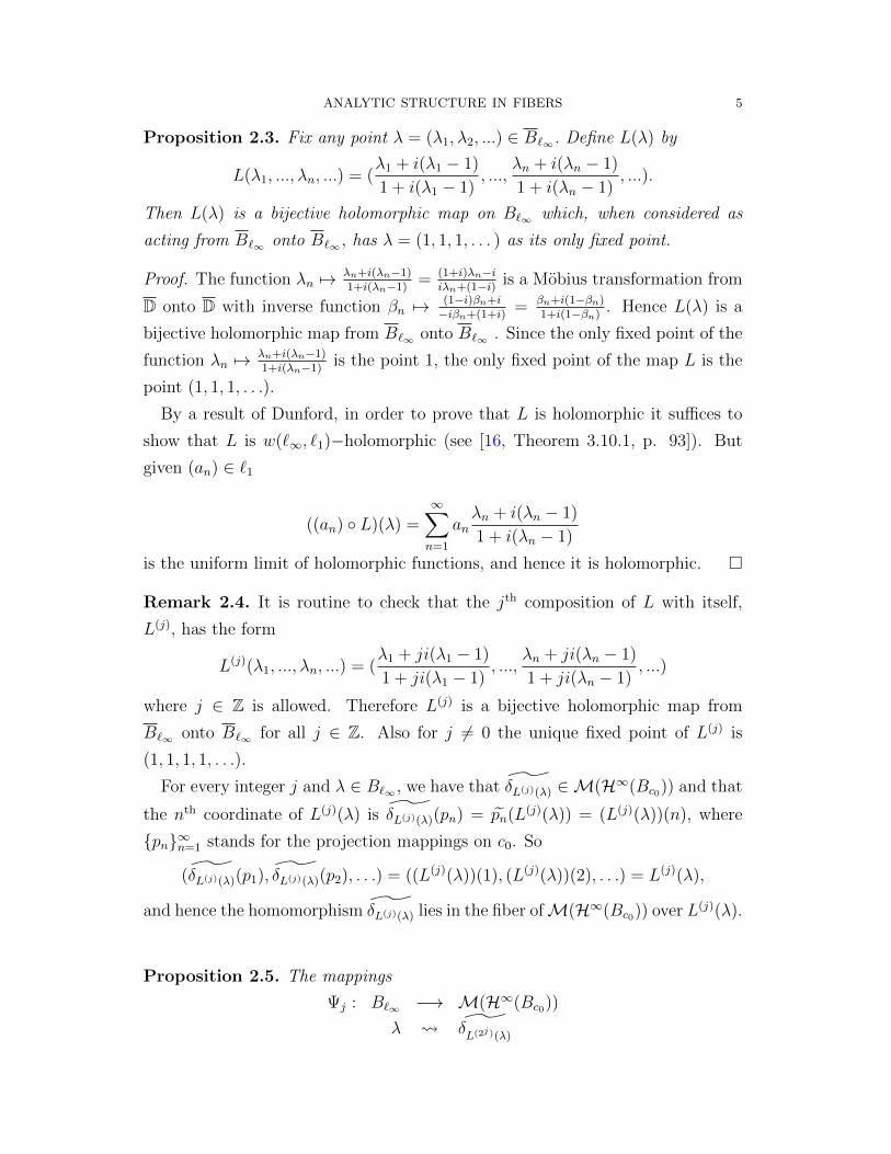
Proposition 2.3. Fix any point λ = (λ1, λ2, ...) ∈ B`∞ . Define L(λ) by

L(λ1, ..., λn, ...) = (λ1 + i(λ1 − 1)

1 + i(λ1 − 1), ...,

λn + i(λn − 1)

1 + i(λn − 1), ...).

Then L(λ) is a bijective holomorphic map on B`∞ which, when considered as

acting from B`∞ onto B`∞ , has λ = (1, 1, 1, . . . ) as its only fixed point.

Proof. The function λn 7→ λn+i(λn−1)1+i(λn−1)

= (1+i)λn−iiλn+(1−i) is a Mobius transformation from

D onto D with inverse function βn 7→ (1−i)βn+i−iβn+(1+i)

= βn+i(1−βn)1+i(1−βn)

. Hence L(λ) is a

bijective holomorphic map from B`∞ onto B`∞ . Since the only fixed point of the

function λn 7→ λn+i(λn−1)1+i(λn−1)

is the point 1, the only fixed point of the map L is the

point (1, 1, 1, . . .).

By a result of Dunford, in order to prove that L is holomorphic it suffices to

show that L is w(`∞, `1)−holomorphic (see [16, Theorem 3.10.1, p. 93]). But

given (an) ∈ `1

((an) ◦ L)(λ) =∞∑n=1

anλn + i(λn − 1)

1 + i(λn − 1)

is the uniform limit of holomorphic functions, and hence it is holomorphic. �

Remark 2.4. It is routine to check that the jth composition of L with itself,

L(j), has the form

L(j)(λ1, ..., λn, ...) = (λ1 + ji(λ1 − 1)

1 + ji(λ1 − 1), ...,

λn + ji(λn − 1)

1 + ji(λn − 1), ...)

where j ∈ Z is allowed. Therefore L(j) is a bijective holomorphic map from

B`∞ onto B`∞ for all j ∈ Z. Also for j 6= 0 the unique fixed point of L(j) is

(1, 1, 1, 1, . . .).

For every integer j and λ ∈ B`∞ , we have that δL(j)(λ) ∈M(H∞(Bc0)) and that

the nth coordinate of L(j)(λ) is δL(j)(λ)(pn) = pn(L(j)(λ)) = (L(j)(λ))(n), where

{pn}∞n=1 stands for the projection mappings on c0. So

(δL(j)(λ)(p1), δL(j)(λ)(p2), . . .) = ((L(j)(λ))(1), (L(j)(λ))(2), . . .) = L(j)(λ),

and hence the homomorphism δL(j)(λ) lies in the fiber ofM(H∞(Bc0)) over L(j)(λ).

Proposition 2.5. The mappings

Ψj : B`∞ −→ M(H∞(Bc0))

λ ˜δL(2j)(λ)


j = 1, 2, . . . are holomorphic of norm one, when considering M(H∞(Bc0)) as a

subset of(H∞(Bc0)

)∗.

Proof. It is enough to check that for each f ∈ H∞(Bc0) the function Ψj(·)(f) ∈H∞(B`∞). For this, notice that for each f ∈ H∞(Bc0)) the function

f(L(2j)) : B`∞ −→ Cλ f(L(2j)(λ))

is the composition of two holomorphic functions, since f ∈ H∞(B`∞) and by

Proposition 2.3 L(2j), is holomorphic. Therefore f(L(2j)) is holomorphic.

Also Ψj has norm one since for every λ ∈ B`∞ , ˜δL(2j)(λ)

∈M(H∞(Bc0)). Hence

‖˜δL(2j)(λ)

‖ = 1.

�

An application of the Ascoli theorem yields that the set of holomorphic map-

pings from B`∞ toM(H∞(Bc0)) is compact with the compact open topology. In

particular the sequence (Ψj)j∈N has at least one accumulation point Ψ : B`∞ →M(H∞(Bc0)) that is also holomorphic.

Proposition 2.6. Any accumulation point Ψ of the sequence (Ψj)j∈N is such that

Ψ(λ) is in the fiber over the point ~1 = (1, 1, ..., 1, ...) ∈ `∞ for every λ ∈ B`∞ . In

particular, Ψ 6= Ψj for j ∈ N.

Proof. We want to check that Ψ(λ) ∈ π−1(~1), i. e. Ψ(λ)(pn) = 1 for all projection

mappings pn. We will check that for every point y = (y1, y2, ..., yn, ...) ∈ `1,

Ψ(λ)(y) =∑

n yn = ~1(y). Therefore, π(Ψ(λ)) = ~1.

Fix y = (y1, y2, ..., yn, ...) ∈ `1. Since Ψ is an accumulation point of (Ψj), there

exists a subnet (Ψα) convergent to Ψ. Since, for each fixed λ, the sequence{λn+2ji(λn−1)1+2ji(λn−1)

}∞j=1

converges to 1, then the subnet{λn+2αi(λn−1)

1+2αi(λn−1)

}α

also converges

to 1. Hence, since y ∈ `1, we have

Ψ(λ)(y) = limα

Ψα(λ)(y) = limα

∞∑n=1

ynλn + 2αi(λn − 1)

1 + 2αi(λn − 1)=∞∑n=1

yn.

Indeed, given ε > 0 there exists n0 ∈ N such that∑

n≥n0|yn| < ε

2. Now the

convergence of{λn+2αi(λn−1)

1+2αi(λn−1)

}α

to 1 for n = 1, . . . , n0 gives the existence of α0

such that∞∑n=1

|yn||1−λn + 2αi(λn − 1)

1 + 2αi(λn − 1)| < ε,


for every α ≥ α0.

Thus Ψ(λ)(y) =∑∞

n=1 yn. Therefore Ψ(λ) ∈ π−1(1).

To finish let us show that Ψ 6= Ψj for all j ∈ N. Observe that |Ψj(λ)(pn)| =

|˜δL(2j)(λ)

(pn)| = |(L(2j)(λ)

)(n)| < 1 for all n, j ∈ N so we have that Ψj(λ) /∈ π−1(~1)

and the result follows. �

Proposition 2.7. Given an accumulation point Ψ of the sequence (Ψj)j∈N, Ψ

takes B`∞ homeomorphically into M~1(H∞(Bc0)) = π−1(~1).

Proof. Define h : B`∞ → B`∞ as follows:

h(λ1, λ2, ..., λn, ...) =

= (λ1Π∞k=0

λ1 − 2ki(λ1 − 1)

1− 2ki(λ1 − 1), ..., λnΠ∞k=0

λn − 2ki(λn − 1)

1− 2ki(λn − 1), ...)

= (λ1Π∞k=0L(−2k)(λ)(1), ..., λnΠ∞k=0L

(−2k)(λ)(n), ...).

Observe that h : Bc0 → Bc0 .

Notice that for every r, 0 < r < 1, and every natural number n, the product

Π∞k=0λn−2ki(λn−1)1−2ki(λn−1)

converges uniformly on the complex disk rD, since

∣∣L(−2k)(λ)(n)− 1∣∣ ≤ Kr

1

2k

for some constant Kr. Therefore the product converges and since |λn−2ki(λn−1)1−2ki(λn−1)

| ≤1 we have

∣∣λnΠ∞k=0

λn − 2ki(λn − 1)

1− 2ki(λn − 1)

∣∣ ≤ |λn|.Hence h is well defined.


Now, for every coordinate and for every complex disk of radius 0 < r < 1 we

have

|h(L(2m)(λ))(n)− λn| = |L(2m)(λ)(n)∞∏k=0

L(−2k)(L(2m)(λ))(n)− λn|

= |L(2m)(λ)(n)∞∏k=0

L(2m−2k)(λ)(n)− λn|

= |λn|∣∣∣L(2m)(λ)(n)

m−1∏k=0

L(2m−2k)(λ)(n)∞∏

k=m+1

L(2m−2k)(λ)(n)− 1∣∣∣

≤ |λn|[|L(2m)(λ)(n)− 1|+

∞∑k=0k 6=m

|L(2m−2k)(λ)(n)− 1|]

≤ |λn|Kr

[ 1

2m+

m−1∑k=0

1

2m − 2k+

∞∑k=m+1

1

2k − 2m

]≤ |λn|Kr

m+ 2

2m−1,

and this converges to zero as m goes to infinity.

Let

h : M(H∞(Bc0)) −→ B`∞

φ (φ(p1 ◦ h), φ(p2 ◦ h), φ(p3 ◦ h), . . .

).

Since h is continuous, h is also continuous. Therefore, as Ψ is a cluster point

of the sequence (Ψj)j∈N,

(h ◦Ψ)(λ) = h(Ψ(λ))

= limαh(Ψα(λ))

= limα

(h(L(2α)(λ))(1), h(L(2α)(λ))(2), . . .

)= (λ1, λ2, . . .) = λ.

Then h ◦Ψ = Id on B`∞ .

Hence, Ψ is bijective onto Ψ(B`∞) with inverse being the restriction of h to

the range of Ψ. Since h is continuous, the restriction of h to Ψ(B`∞) is also

continuous. Therefore, Ψ is a continuous bijective map from B`∞ onto Ψ(B`∞)

with continuous inverse h|Ψ(B`∞ ). Thus, Ψ is a homeomorphism. �

Corollary 2.8. Let z0 = (z1, z2, ..., zn, ...) be a point of the boundary of B`∞ such

that there exists n0 with |zn| = 1 for all n > n0. Then there exists an injection

Ψ : B`∞ →Mz0(H∞(Bc0)) which is homeomorphic onto its image.


For the proof of this corollary, we can assume, without loss of generality, that

max{|z1|, . . . , |zn0|} < 1. Now the lemma below and Theorem 2.2 give the con-

clusion.

Lemma 2.9. Given (b1, w0) := (b1, z2, . . . , zn, . . .) ∈ B`∞ with |b1| < 1, we have

that M(b1,w0)(H∞(Bc0)) is homeomorphic to Mw0(H∞(Bc0)).

Proof. Define R :Mw0(H∞(Bc0))→M(b1,w0)(H

∞(Bc0)) by

R(ϕ)(f) = ϕ(w f(b1, w)).

We claim that R has the following properties: R is w∗ − w∗ continuous; R is

one-to-one; and R is onto. Once we have shown these three properties of R, we

will be able to conclude that the fiber over w0 in M(H∞(Bc0)) is topologically

the same as the fiber of (b1, w0) in M(H∞(Bc0)).

For the first, suppose that ϕα → ϕ weak-star in M(H∞(Bc0)). So, for all

h ∈ H∞(Bc0), ϕα(h) → ϕ(h). Fixing f ∈ H∞(Bc0), we see that R(ϕα)(f) =

ϕα(w f(b1, w)) converges to ϕ(w f(b1, w)) = R(ϕ)(f). Thus, R is w∗ − w∗

continuous.

Next, we show that R is one-to-one. Suppose that ϕ1 6= ϕ2 inMw0(H∞(Bc0)).

So, for some h ∈ H∞(Bc0), ϕ1(h) 6= ϕ2(h). Define f ∈ H∞(Bc0) by f(z1, w) =

h(w), for all (z1, w) ∈ Bc0 . Then

R(ϕ1)(f) = ϕ1(w f(b1, w)) = ϕ1(h)

6= ϕ2(h) = ϕ2(w f(b1, w)) = R(ϕ2)(f).

Finally, let’s show that R is onto. So, fix ψ ∈ M(b1,w0)(H∞(Bc0)). Let ϕ :

H∞(Bc0) → C be given by ϕ(h) = ψ((z1, w) h(w)). We claim that R(ϕ) =

ψ. First, π(ϕ) = (xn)∞n=1 where xn = ϕ(en) and en is the n-th element of the

canonical Schauder basis of c∗0 = `1. But, by definition of ϕ

(xn)∞n=1 = (ψ((z1, w) wn))∞n=1 = w0.

This follows since ψ ∈ M(b1,w0)(H∞(Bc0)) implies that π(ψ) = ((ψ((z1, w)

z1, (ψ((z1, w) wn))∞n=1) = (b1, w0). It then follows that

R(ϕ)(f) = ϕ(h : w f(b1, w)) = ψ((z1, w) h(w)) = ψ((z1, w) f(b1, w)).


Next, for a fixed f ∈ H∞(Bc0), define g : Bc0 → C by

g(z1, w) =

{f(z1,w)−f(b1,w)

z1−b1 if z1 6= b1∂f∂z1

(b1, w) if z1 = b1.

The function g is locally bounded and separately holomorphic on the open unit

ball of the Banach space c0 and hence it is holomorphic. Moreover, g is bounded

on Bc0 . To see this, consider z1 in D so that |z1 − b1| ≥ |1−b1|2. Then |g(z1, w)| ≤

2|1−b1|(|f(z1, w)|+ |f(b1, w)|) ≤ 4

|1−b1|‖f‖Bc0 . If 0 < |z1−b1| ≤ |1−b1|2

, since for each

w ∈ Bc0 the function z1 → g(z1, w) is holomorphic on D, the Maximum Modulus

Theorem implies that g attains its maximum at a point of the circle centered at

b1 and of radius |1−b1|2

. Thus, ‖g‖Bc0 ≤4

|1−b1|‖f‖Bc0 , and we have that

f(z1, w) = f(b1, w) + (z1 − b1)g(z1, w),

with g ∈ H∞(Bc0). Using the fact that ψ(g) is well-defined, we see that

ψ(f) = ψ((z1, w) f(b1, w) + (z1 − b1)g(z1, w)) =

= ψ((z1, w) f(b1, w))+ψ((z1, w) (z1−b1)g(z1, w)) = ψ((z1, w)) f(b1, w)),

since ψ((z1, w) z1 − b1) = b1 − b1 = 0. �

Remark 2.10. An argument analogous to that in the proof of Theorem 2.2

implies that there exists an injection Ψ : B`∞ → M(1,0,1,0,...,1,0,...)(H∞(Bc0))

which is biholomorphic onto its image. However, we do not know if the fibers

of M(H∞(Bc0)) over the points (1, 0, 1, 0, . . . , 1, 0, . . .) and (1, 1, . . . , 1, . . .) are

homeomorphic or not. Also we do not know if B`∞ can be embedded in the fiber

M(zn)(H∞(Bc0)), when (zn) is in the unit sphere of `∞ but |zn| < 1 for all n, as

for example (n−1n

).

Remark 2.11. Let us observe that the arguments of the proofs of Corollary 2.8

and Lemma 2.9, can easily be adapted to produce counterpart results for fibers

of the maximal ideal of H∞(D2), the space of bounded holomorphic function on

the bidisk. This finite dimensional approach is part of a work in progress.

Proposition 2.12. For all f ∈ H∞(Bc0) there exists g ∈ H∞(Bc0) such that

Ψ(λ)(g) = f(λ) for all λ ∈ Bc0 .


Proof. Let g = f ◦ h ∈ H∞(Bc0), where h : Bc0 → Bc0 is the function introduced

in Proposition 2.7. Consider

g : M(H∞(Bc0)) −→ Cφ φ(g).

Therefore, for all λ ∈ Bc0 ,

Ψ(λ)(g) ≡ g(Ψ(λ)) = g(limα

Ψα(λ))

= limαg(Ψα(λ)) = lim

α(Ψα(λ))(g) = lim

α˜δL(2α)(λ)(g)

= limα

˜δL(2α)(λ)(f ◦ h) = limαf ◦ h(L(2α)(λ)).

By [9, Corollary 2.2] and using the fact that the space c0 is symmetrically regular

(see, e.g., [1]) we have that f ◦ h(L(2α)(λ)) = (f ◦ h)(L(2α)(λ)). Hence

Ψ(λ)(g) = limαf ◦ h(L(2α)(λ)) = lim

α(f ◦ h)(L(2α)(λ))

= limα

(f ◦ h)(L(2α)(λ)) = f(limα

(h(L(2α)(λ))))

= f(λ) = f(λ).

�

Now, proceeding analogously to [19], we can use Ψ to transfer the analytic

structure of B`∞ into Ψ(B`∞). In this way, for every function f ∈ H∞(Bc0) we

can consider the extension f ∈ H∞(B`∞). Since M(H∞(Bc0)) ⊆ S(H∞(Bc0 ))∗ , the

restriction of f to Ψ(B`∞) is a bounded analytic function on Ψ(B`∞).

In other words, we can say that if B :≡ H∞(Ψ(B`∞)) is endowed with the

supremum norm, then B is a uniformly closed Banach algebra of continuous

function on Ψ(B`∞), which is isomorphic to H∞(Bc0). Then, the maximal ideal

space of B is

M(B) = {φ ∈M(H∞(Bc0));φ(f) = 0 whenever f = 0 on Ψ(B`∞)}.

Therefore the maximal ideal space can be identified with M(H∞(Bc0)). Hence

the fiber Mz(H∞(Bc0)), for any z in Tℵ0 , contains a homeomorphic copy of

M(H∞(Bc0)).

Roughly speaking, the maximal ideal space M(H∞(Bc0)) reproduces itself ad

infinitum inside each of the fibers Mz(H∞(Bc0)) for any z in Tℵ0 .

Recently, Johnson and Ortega Castillo [18] studied some properties of the fibers

of the maximal ideal space of the Banach algebra H∞(BC(K)), when K is a


scattered Hausdorff compact set and C(K) is the space of continuous complex

valued function on K. We are going to show that these results can be translated

to some of the fibers of M(H∞(BC(K))).

Recall that a Hausdorff compact set K is called scattered (or dispersed) if every

point has a basis of clopen neighborhoods. Hence if K is infinite it is always

possible to find a sequence (Un) of pairwise disjoint, non-empty clopen subsets.

Observe that χUn belongs to C(K) for every n.

Lemma 2.13. Let K be an infinite scattered compact Hausdorff set and let (Un)

be a sequence of non empty clopen sets pairwise disjoint subsets of K. Let Φ :

c0 → C(K) be defined by

Φ((an)) =∞∑n=1

anχUn .

(i) The mapping R :M(H∞(Bc0))→M(H∞(BC(K))),

R(ϕ)(F ) = ϕ(F ◦ Φ)

is an injective and holomorphic mapping, for every ϕ in M(H∞(Bc0)) and every

F in H∞(BC(K)).

(ii) If z = (bn) belongs to the closed unit ball of `∞ and we consider∑∞

n=1 bnχUn

as an element of the closed unit ball of C(K)∗∗, then

R(M(bn)(H∞(Bc0))) ⊂M∑∞n=1 bnχUn

(H∞(BC(K))).

Proof. Clearly∑∞

n=1 anχUn is continuous on K for any null sequence (an) and

‖∑∞

n=1 anχUn‖ = ‖(an)‖. Hence Φ is well-defined and is a linear isometry. As a

consequence T : H∞(BC(K)) → H∞(Bc0), T (F ) = F ◦ Φ, is also well-defined

and continuous. Thus T ∗ : H∞(Bc0)∗ → H∞(BC(K))

∗ is linear and contin-

uous too (therefore an entire function). Moreover, since T is multiplicative,

T ∗(M(H∞(Bc0)) ⊂M(H∞(BC(K))). Since R is the restriction of the mapping T ∗

toM(H∞(Bc0)) to finish the proof of (i), we only have to check that R is injective.

For that consider ϕ inM(H∞(Bc0)) and let g ∈ H∞(Bc0) with ϕ(g) 6= 0. As be-

fore, denote by g in H∞(B`∞) the canonical extension of g and choose tn in Un for

every n. Given h in BC(K), as (h(tn)) is in B`∞ , we can define F0(h) = g(h(tn)).

Clearly F0 belongs to H∞(BC(K)) and

R(ϕ)(F0) = ϕ(g) 6= 0.


(ii) If L is in C(K)∗, and z = (an) is any element of Bc0 , then

L ◦ Φ((an)) = L(∞∑n=1

anχUn) =∞∑n=1

anL(χUn).

Hence, the sequence (L(χUn)) is in `1 and 〈L,∑∞

n=1 bnχUn〉 :=∑∞

n=1 bnL(χUn)

defines a continuous linear form on C(K)∗ for each z = (bn) in B`∞ . Now, for

fixed (bn) ∈ B`∞ , if ϕ is in M(bn)(H∞(Bc0)), then

π(R(ϕ))(L) = ϕ(L ◦ Φ) = ϕ(L(χUn)) =∞∑n=1

bnL(χUn),

for every L in C(K)∗ and (ii) is proved. �

Corollary 2.14. Let K be an infinite scattered compact Hausdorff set. The

following hold:

(i) B`∞ is continuously injected in the fiber M0(H∞(BC(K))).

(ii) There exists an injection from B`∞ into M∑∞n=1 χUn

(H∞(BC(K))), which is

biholomorphic onto its image.

Proof. (i) is a consequence of [10, 6.7 Theorem] and of Lemma 2.13.(ii).

(ii) in turn, is a consequence of Theorem 2.2 and of Lemma 2.13.(ii). �

3. Disks in fibers of the algebra of the ball of a Banach space

The main goal of this section is to prove the following theorem.

Theorem 3.1. Let X be a Banach space such that there exists a polynomial P

and x0 ∈ BX such that P |BX is not weakly continuous at x0. Then the complex

disk D can be analytically injected in Mz(Au(BX)) for every z ∈ BX∗∗.

Remark 3.2. It might well seem that this unprepossessing result treats a very

special situation and is therefore of little interest. In fact, the condition in The-

orem 3.1 is close to being necessary and sufficient, in the following sense. If it

happens that every polynomial is weakly continuous at each point of BX and X∗

has the approximation property, by using a similar argument to [5, Theorem 7.2]

we have Mz(Au(BX)) = {δz} for every z ∈ BX∗∗ . Hence the fibers contains no

disk at any point in the open unit ball of the bidual of X. It is unknown if the

same holds if X∗ does not have the approximation property.


Also it is worth recalling that for many Banach spaces, the fiberMx(Au(BX))

at any point x in the unit sphere of X is reduced to the evaluation at x. This can

occur even in the case that the space has a polynomial whose restriction to the

corresponding unit ball is not weakly continuous at any point. Examples of such

spaces include the uniformly convex spaces, (consequence of [15, Proposition 4.1]

and [3, Lemma 2.4], see also the remark preceding [4, Corollary 2.3]). Another

example is `1 [4, Proposition 3.1].

In order to prove Theorem 3.1 we first need to study the set of points in which

a continuous polynomial P defined on a complex Banach space is discontinuous

when restricted to bounded sets that are endowed with a weaker topology than

the norm. Our discussion is related to [6] and [7].

Given x ∈ X and r > 0, BX(x, r) will stand for the open ball centered at x

with radius r.

Lemma 3.3. Let U be an open subset of a Banach space X and f ∈ H(U). Let

E be a subset of X∗ separating points of X. If for some x0 ∈ U there exists r > 0

such that BX(x0, r) ⊂ U and f |BX(x0,r) is w(X,E)-continuous at x0 then, for each

n ∈ N and R > 0, the mapping x dnfn!

(x0)(x) is w(X,E)-continuous at 0 when

restricted to BX(0, R).

Proof. Let us write Pn(x) := dnfn!

(x0)(x), x ∈ X, so Pn is a continuous n-

homogeneous polynomial that is the nth Taylor coefficient of f at x0. It is routine

that

Pn(x) =1

2πi

∫|λ|=1

f(x0 + λx)

λn+1dλ

if ‖x‖ < r.

By hypothesis, given ε > 0 there exist x∗1, . . . , x∗k ∈ E and 0 < δ < r such that

supj=1,...,k |x∗j(x)| < δ implies that |f(x0 + x)− f(x0)| < ε. It follows that

|Pn(x)− Pn(0)| =∣∣∣ 1

2πi

∫|λ|=1

f(x0 + λx)− f(x0)

λn+1dλ∣∣∣

≤ max|λ|=1|f(x0 + λx)− f(x0)| < ε ,

for every x ∈ B(0, r) such that supj=1,...,k |x∗j(x)| < δ.

Now, if (xα)α∈Λ is a net that is w(X,E)-convergent to 0 in RBX = BX(0, R),

then ( rRxα)α∈Λ is in BX(0, r) and is also w(X,E)-convergent to 0. Thus Pn(xα) =


(Rr)nPn( r

Rxα) is w(X,E)-convergent to (R

r)nPn(0) = 0 = Pn(0). Therefore,

Pn|RBX is w(X,E)-continuous at 0 for every R > 0 and every n ∈ N. �

Proposition 3.4. Let R > 0 and let E ⊂ X∗ separate points of X. If P : X −→ Cis a continuous polynomial that is not w(X,E)-continuous at x0 ∈ BX(0, R) when

restricted to the open ball BX(0, R) then, for every r > 0 such that BX(x0, r) ⊂BX(0, R), P |BX(x0,r) is not w(X,E)-continuous at x0.

Proof. We can write P (x0 + x) = P (x0) +∑m

j=1 Pj(x), for every x ∈ X, where m

is the degree of P and each Pj : X → C is a j-homogeneous polynomial. If r0 > 0

were such that BX(x0, r0) ⊂ BX(0, R) and P |BX(x0,r0) is w(X,E)-continuous at

x0 then, by Lemma 3.3, each Pj (j = 1, . . . ,m) would be w(X,E)-continuous at

0 when restricted to BX(0, R). Hence P |BX(0,R) would be w(X,E)-continuous at

x0, a contradiction. �

Proposition 3.5. If P : X −→ C is an m-homogeneous continuous polynomial

that is not w(X,E)-continuous at 0 when restricted to the unit ball BX then,

for every x ∈ BX and every r > 0 such that BX(x, r) ⊂ BX , P |BX(x,r) is not

w(X,E)-continuous at x. Here, as above, E ⊂ X∗ separates points of X.

Proof. By Proposition 3.4, it is enough to prove that for each x in BX , P |BX is

not w(X,E)-continuous at x.

Here we follow the idea of the proofs of Boyd-Ryan [7, Proposition 1] and [7,

Corollary 2]. First we will show that the set of points where P |BX is w(X,E)-

continuous is closed in norm. Let (xn)n∈N be a sequence of points convergent in

norm to x0, where for each n, P |BX is w(X,E)-continuous at xn. Let ε > 0 and

(yα)α∈A be a bounded net that is w(X,E)-convergent to 0 with x0 +yα, xn+yα ∈BX for all n ∈ N. Since P is an m-homogeneous continuous polynomial, P is

uniformly continuous when restricted to BX . Then there exists nε ∈ N such that

|P (x0)−P (xn)| ≤ ε/3 and |P (x0 + yα)−P (xn + yα)| ≤ ε/3 for all n ≥ nε and for

all α ∈ A. Also since P is w(X,E)-continuous at xnε there exists αε such that

|P (xnε + yα)− P (xnε)| ≤ ε/3 for all α ≥ αε. It follows that

|P (x0 + yα)− P (x0)| ≤ ε,

for all α ≥ αε, and so the set of points where P |BX is w(X,E)-continuous is

closed.


Let us now show that P |BX is not w(X,E)-continuous at any point x ∈ BX . So,

suppose that for some x0 ∈ BX , P |BX is w(X,E)−continuous at x0. Hence, for

any r > 0 satisfying BX(x0, r) ⊂ BX , P |BX(x0,r) is w(X,E)−continuous at x0. Fix

n ∈ N and apply the contrapositive of Proposition 3.4 to P and the case R = n.

It follows that P |nBX is w(X,E)−continuous at x0. Hence, by homogeneity, P |BXis w(X,E)−continuous at 1

nx0. However, since the set of points where P |BX is

w(X,E)−continuous is closed, it follows that P |BX is w(X,E)−continuous at 0,

which contradicts the hypothesis. Therefore P |BX is not w(X,E)-continuous at

any x ∈ BX . �

Typical examples of subsets E satisfying the hypotheses of the preceding results

are E = X∗ or E = Y whenever X = Y ∗.

Now, we translate the above results to the two weak topologies that are of

greatest interest to us, the weak w(X,X∗) and the weak-star w(X∗∗, X∗). It must

be pointed out that the following Corollary complements results of V. Dimant,

such as Corollary 1.7 and Remark 1.8 in [13].

Corollary 3.6. If P : X −→ C is an m-homogeneous continuous polynomial

that is not weakly continuous at 0 when restricted to the unit ball BX then the

following hold,

(1) For every x ∈ BX and every r > 0 such that BX(x, r) ⊂ BX , P |BX(x,r) is

not weakly continuous at x.

(2) For every z ∈ BX∗∗ and every r > 0 such that BX∗∗(z, r) ⊂ BX∗∗, the

canonical extension P |BX∗∗ (z,r) of P is not weak-star continuous at z.

Proof. (1) Apply Proposition 3.5 for the space X and E = X∗.

(2) Apply Proposition 3.5 for the space X∗∗ and E = X∗ ⊂ X∗∗∗ and use

the fact that P is not w(X∗∗, X∗)-continuous at 0 whenever P is not weakly

continuous at 0 (restricted to the corresponding unit balls). �

Corollary 3.6 above is a refinement of Proposition 1, Corollary 2 and Proposi-

tion 3 of [7]. Also the results from Lemma 3.3 to Example 3.9 could be stated in

terms of weakly sequential continuity of polynomials, in which case Corollary 3.6

is related to Proposition 1.(1) and 1.(2) of [6].

Corollary 3.7. Let X be a Banach space, x0 ∈ BX , 0 < r < 1 − ‖x0‖, and

f ∈ Au(BX) such that f |BX(x0,r) is not weakly continuous at x0. Then there


exists an m-homogeneous continuous polynomial P such that P |BX is not weakly

continuous at any point of BX , and the canonical extension P |BX∗∗ is not weak-

star continuous at any point of BX∗∗.

Proof. Let Pn := dnfn!

(x0), n ∈ N. We have that∑∞

m=0 Pm(x − x0) converges

absolutely and uniformly to f on BX(x0, r). If every Pm were weakly continuous

at 0 (restricted to any ball centered at 0) then by uniform convergence f |BX(x0,r)

would be weakly continuous at x0. Now the conclusion follows from Corollary

3.6. �

Proposition 3.8. Let X be a complex Banach space and P : X 7→ C be a contin-

uous polynomial of degree m. If G := {x ∈ BX : P |BX is weakly continuous at x}has nonempty interior then P restricted to bounded sets is weakly continuous.

Proof. Let x0 ∈ G and r > 0 such that BX(x0, r) ⊂ G ⊂ BX . Then

P (x0 + u) = P (x0) +m∑n=1

dnP

n!(x0)(u),

for all u ∈ BX(0, r).

Applying the Cauchy integral formula for u, u0 ∈ BX(0, r), we get

Pn(u)− Pn(u0) =1

2πi

∫λ=1

P (x0 + λu)− P (x0 + λu0)

λn+1dλ.

Fix u0 ∈ BX(0, r). By the weak continuity of P |BX at any point of BX(x0, r),

given ε > 0, for each λ ∈ C with |λ| = 1 there exist a finite set Aλ ⊂ X∗

and a positive number δλ such that if x − (x0 + λu0) is in the weakly open set

Vλ := {y ∈ BX : supx∗∈Aλ |x∗(y)| < δλ} and x ∈ BX then

(3.1) |P (x)− P (x0 + λu0)| < ε/2.

By the compactness of the set {λu0 : |λ| = 1} there exist complex numbers

λ1, . . . , λp of modulus one such that {λu0 : |λ| = 1} ⊂ ∪pl=1

(λlu0 + 1

2Vλl). Let

A = ∪pl=1Aλl , δ = min{12δλl : l = 1, . . . , p} and denote by V := {y ∈ BX :

supx∗∈A |x∗(y)| < δ}. Notice V ⊂ 12Vλl for l = 1, . . . , p.

Given a complex number λ of modulus one there exists l ∈ {1, . . . , p} with

λu0 ∈ λlu0 +1

2Vλl .

Therefore (x0 +λu0)− (x0 +λlu0) = λu0−λlu0 ∈ 12Vλl ⊂ Vλl . Hence by equation

(3.1) we have

(3.2) |P (x0 + λu0)− P (x0 + λlu0)| < ε/2.


Also, for every u ∈ BX such that u− u0 ∈ V, we have λu− λu0 = λ(u− u0) ∈λV = V ⊂ 1

2Vλl ⊂ Vλl . Hence (x0 + λu)− (x0 + λlu0) = λu− λlu0 ∈ Vλl , and by

equation (3.1) again

(3.3) |P (x0 + λu)− P (x0 + λlu0)| < ε/2.

Then, by the triangle inequality and equations (3.2) and (3.3)

|P (x0 + λu)− P (x0 + λu0)| < ε.

Therefore for every u ∈ BX(0, r)

|Pn(u)− Pn(u0)| = 1

2πi|∫λ=1

P (x0 + λu)− P (x0 + λu0)

λn+1dλ|

≤ max|λ|=1|P (x0 + λu)− P (x0 + λu0)| ≤ ε.

Thus the n-homogeneous polynomial Pn|BX(0,r) = dnPn!

(x0) is weakly continuous at

u0, for all u0 in BX(0, r). Since Pn is a continuous n-homogeneous polynomial, we

have that the restriction of Pn to bounded sets is weakly continuous. Therefore

P (x) = P (x0)+P1(x−x0)+ · · ·+Pm(x−x0) restricted to bounded sets is weakly

continuous. �

To finish our study of weakly continuity of polynomials we would like to point

out the following example, that shows that even if the homogeneous parts of a

polynomial are non-weakly continuous, the polynomial itself need not be non-

weakly continuous.

Example 3.9. Consider a Banach space X and a k-homogeneous polynomial Q

such that the restriction of Q to BX is not weakly continuous at some x0 6= 0.

Then, there are non-homogeneous polynomials P = P1 + · · · + Pm with Pj ∈P(njX), n1 < n2 < · · · < nm such that P |BX is weakly continuous at x0 but none

of the Pj|BX are weakly continuous at x0.

Proof. Consider x∗0 in X∗ such that x∗0(x0) = 1 and an arbitrary but fixed natural

number h. Define the polynomial

P (x) :=(1− x∗0(x)

)hQ(x) =

h∑j=0

(h

j

)(−x∗0(x))jQ(x), x ∈ X.

Then P is a non-homogeneous polynomial of degree k + h with homogeneous

parts(hj

)(−x∗0(x))jQ(x) ∈ P(j+kX), for j = 1, . . . , h, such that their restrictions

to BX are not weakly continuous at x0.


However,

|P (x)− P (x0)| = |(1− x∗0(x)

)hQ(x)| ≤

∣∣1− x∗0(x)∣∣h‖Q‖.

Hence if a net (xα) ⊂ BX weakly converges to x0 we have that∣∣1 − x∗0(x)

∣∣hconverges to zero. Thus P |BX is weakly continuous at x0. �

We are now ready to prove the main theorem of this section.

Proof of Theorem 3.1. By Corollary 3.7, there exists an m-homogeneous contin-

uous polynomial Q such that the restriction of its canonical extension Q to BX∗∗

is not w(X∗∗, X∗)-continuous at any point of z ∈ BX∗∗ .

Fix z0 ∈ BX∗∗ and 0 < r < 1−‖z0‖. By Proposition 3.4, Q|BX∗∗ (z0,r) is not w∗-

continuous at z0. Hence there is a net (zλ)λ∈Λ ⊂ BX∗∗(z0, r) that is w∗-convergent

to z0 such that

Q(zλ) 9 Q(z0) .

Taking a subnet, and not changing the notation, we have for some ε > 0 that

(3.4) |Q(zλ)− Q(z0)| ≥ ε ,

for all λ ∈ Λ. Let U be an ultrafilter on Λ such that U ⊃ {{µ ∈ Λ : µ ≥ λ} : λ ∈Λ} and define

Φ : D −→Mz0(Au(BX))

by

Φ(t)(f) := limλ∈U

f(z0 + t(zλ − z0))

for all t ∈ D and all f ∈ Au(BX).

It is routine to verify that Φ(t) ∈Mz0(Au(BX)) for all t ∈ D.

Since Q is polynomial of degree m

Q(z0 + t(zλ − z0)) = Q(z0) +m∑j=1

Qj(t(zλ − z0)) = Q(z0) +m∑j=1

tjQj(zλ − z0).

Hence

Φ(t)(Q) = limλ∈U

Q(z0 + t(zλ − z0)) = Q(z0) +m∑j=1

tj limλ∈U

Qj(zλ − z0) =m∑j=0

ajtj ,

where a0 := Q(z0) and aj := limλ∈U Qj(zλ − z0) for j = 1, . . . ,m.

Thus, the mapping t Φ(t)(Q) (t ∈ D) is the restriction to D of the polynomial∑mj=0 ajt

j. But Φ(0)(Q) = Q(z0) and by (3.4) |Φ(1)(Q) − Q(z0)| ≥ ε. So the

one variable polynomial t Φ(t)(Q) is non-constant and has degree less than


or equal to m. Therefore we can find a point t0 ∈ D and s > 0 such that

D(t0, s) := t0 + sD ⊂ D and g(t) : D(t0, s) −→ C, defined by g(t) = Φ(t)(Q) for

all t ∈ D(t0, s) is injective.

We claim that h : D −→ Mz0(Au(BX)) defined by h(u) = Φ(t0 + su), for all

u ∈ D, is injective and analytic on D. By the above it is injective. Let us show

that it is also analytic. Given f ∈ Au(BX), we have

f ◦ Φ(t) = Φ(t)(f) = limλ∈U

f(z0 + t(zλ − z0)) ,

where f stands for the Gelfand transform of f . For λ ∈ Λ, define fλ : D −→ C by

fλ(t) := f(z0 + t(zλ − z0)) (t ∈ D). Consider now the family F := {fλ : λ ∈ Λ}.This is a subset of ‖f‖∞BH∞(D) which is a relatively compact subset of the space

H(D) of holomorphic functions on D, with respect to the compact-open topology.

Hence there exists g ∈ ‖f‖∞BH∞(D) such that g = limλ∈U fλ. Obviously g(t) =

limλ∈U fλ(t) = f ◦ Φ(t), for all t ∈ D. Thus Φ is analytic on D and therefore h is

analytic on D as well. �

In certain special cases, the conclusion of Theorem 3.1 can be considerably

strengthened. One such situation follows.

Proposition 3.10. For every 1 < p < ∞ the closed unit ball of `p can be con-

tinuously injected into M0(Au(B`p)). Moreover, the restriction of that injection

to the open unit ball of `p is analytic.

Proof. We split N =⋃∞n=1 Jn with Card(Jn) = Card(N) for all n ∈ N, Jn

⋂Jm = ∅

for n 6= m and Jn ⊂ {n, n+ 1, . . .} for all n ∈ N.

Now we write Jn = (i(n,k))∞k=1 such that n ≤ i(n,1) < i(n,2) < . . . < i(n,k) <

i(n,k+1) < . . . , and for a fixed (λn)n∈N ∈ B`p we define

ϕk := δ∑∞n=1 λnei(n,k)

(k ∈ N) .

Let U be a free ultrafilter on N and define

ϕ(λn)n∈N(f) := limk∈U

ϕk(f) (f ∈ Au(B`p)) .

The sequence(∑∞

n=1 λnei(n,k)

)∞k=1

is weakly convergent to 0, as it is contained

in the closed unit ball of `p and the support of each∑∞

n=1 λnei(n,k) is contained

in {k, k + 1, . . .}. Hence, ϕ(λn)n∈N ∈M0(Au(B`p)) for every (λn)n∈N ∈ B`p . Thus

the mapping

Φ : B`p −→M0(Au(B`p))


defined by Φ((λn)n∈N) = ϕ(λn)n∈N ((λn)n∈N ∈ B`p)), is well-defined. Let us now

see that it is injective.

Fix n0 ∈ N and define the two polynomials

P (x) =∞∑k=1

xbpc+1i(n0,k)

, Q(x) =∞∑k=1

xbpc+2i(n0,k)

, (x = (xn)n∈N ∈ `p)

where bpc is the integer part of p. Since for r ≥ p and every x = (xn)n∈N ∈ B`p

we have that∑∞

k=1

∣∣xi(n0,k)∣∣r ≤∑∞k=1

∣∣xi(n0,k)∣∣p ≤ 1, the polynomials P and Q are

in Au(B`p).

Suppose Φ((λn)n∈N) = Φ((µn)n∈N) for some (λn)n∈N, (µn)n∈N ∈ B`p . Then

ϕ(λn)n∈N(P ) = ϕ(µn)n∈N(P ) ,

but

ϕ(λn)n∈N(P ) = limk∈U

ϕk(P ) = limk∈U

δ∑∞n=1 λnei(n,k)

(P )

= limk∈U

P( ∞∑n=1

λnei(n,k))

= limk∈U

λbpc+1n0

= λbpc+1n0

.

Analogously, ϕ(µn)n∈N(P ) = µbpc+1n0 and also ϕ(λn)n∈N(Q) = λ

bpc+2n0 , ϕ(µn)n∈N(Q) =

µbpc+2n0 and ϕ(λn)n∈N(Q) = ϕ(µn)n∈N(Q) . Therefore 0 = λbpc+1

n0− µbpc+1

n0= (λn0 − µn0)(λ

bpcn0

+ λbpc−1n0

µn0 + · · ·+ µbpcn0),

0 = λbpc+2n0

− µbpc+2n0

= (λn0 − µn0)(λn0(λ

bpcn0

+ λbpc−1n0

µn0 + · · ·+ µbpcn0) + µbpc+1

n0

).

These equalities imply that λn0 = µn0 . Since n0 is arbitrary the conclusion follows.

We still must prove that for every f ∈ Au(B`p) the mapping f ◦ Φ : B`p → Cis uniformly continuous on B`p and holomorphic on B`p , where f stands for the

Gelfand transform of f . The uniformly continuity of f ◦ Φ is obvious, since

given ε > 0 there exists δ > 0 such that if x, y ∈ B`p satisfy ‖x − y‖ < δ then

|f(x)− f(y)| < ε. Since ‖∑∞

n=1 xnei(n,k) −∑∞

n=1 ynei(n,k)‖ = ‖x− y‖, for every k,

we obtain that

|Φ((xn))(f)− Φ((yn))(f)| ≤ ε,

for every x, y ∈ B`p . As f ◦ Φ is continuous on B`p , in order to prove that it is

holomorphic it is enough to check that it is Gateaux holomorphic on B`p (see,

e.g. [14, Proposition 3.7, pag. 153]). Let x0 = (xn) ∈ B`p , y0 = (yn) ∈ `p \ {0},


and let r > 0 be such that ‖x0‖+ r‖y0‖ < 1. Given k, one sees that

‖∞∑n=1

xnei(n,k)‖+ r‖∞∑n=1

ynei(n,k)‖ = ‖x0‖+ r‖y0‖ < 1.

If we denote by (Pm(z)) the sequence of m-homogeneous polynomials that are

the Taylor coefficients of f at z in the open unit ball, we will have

f(∞∑n=1

xnei(n,k) + t

∞∑n=1

ynei(n,k)) =∞∑m=0

tmPm(∞∑n=1

xnei(n,k))(∞∑n=1

ynei(n,k)),

for every t ∈ C with |t| < r. Moreover, by the Cauchy inequalities,

rm|Pm(∞∑n=1


ynei(n,k))| ≤ sup{|f(x)| : ‖x‖ ≤ ‖x0‖+ r‖y0‖} <∞,

for every m and k. Hence,

Φ(x0 + ty0)(f) =∞∑m=0

tm limk∈U

Pm(∞∑n=1


ynei(n,k)),

for every t ∈ C with |t| < r and the conclusion follows. �

References

[1] R. Arens, The adjoint of a bilinear operation. Proc. Amer. Math. Soc. no. 2, (1951), 839–848.[2] R. M. Aron, P. D. Berner, A Hahn-Banach extension theorem for analytic mappings. Bull.Soc. Math. France 106 (1978), no. 1, 3–24.

[3] R. M. Aron, D. Carando, T.W. Gamelin, S. Lassalle, M. Maestre, Cluster values of analyticfunctions on a Banach space. Math. Ann. 353 (2012), 293–303.

[4] R. M. Aron, D. Carando, S. Lassalle, M. Maestre, Cluster values of holomorphic functionsof bounded type. Trans. Amer. Math. Soc. 368, no. 4 (2016), 2355–2369.

[5] R. M. Aron, B. Cole, T. Gamelin, Weak-star continuous analytic functions. Canad. J. Math.47 (1995), 673–683.

[6] R. M. Aron, V. Dimant, Sets of weak sequential continuity for polynomials. Indag. Math.13 (2002), 287–299.

[7] C. Boyd, R. A. Ryan, Bounded weak continuity of homogeneous polynomials at the origin.Arch. Math. (Basel) 71 (1998), no. 3, 211–218.

[8] D. Carando, D. Garcıa, M. Maestre, P. Sevilla, On the spectra of algebras of analytic func-tions. Contemporary Mathematics 561 (2012) 165–198.

[9] Y. S. Choi, D. Garcıa, S. G. Kim, M. Maestre, Composition, numerical range and Aron-Berner extension. Math. Scand. 103(1), (2008) 97–110.

[10] B. Cole, T. W. Gamelin, W. B. Johnson, Analytic disks in fibers over the unit ball of aBanach space. Michigan Math. J. 39 (1992), no. 3, 551–569.

[11] W. Cutrer, On analytic structure in the maximal ideal space of H∞(Dn). Illinois J. Math.16 (1972), 423–433.

[12] A. M. Davie, T. W. Gamelin, A theorem on polynomial-star approximation. Proc. Amer.Math. Soc. 106 (1989), 351–356.

[13] V. Dimant, M−ideals of homogeneous polynomials, Studia Math. 202 (1) (2011), 81–102.[14] S. Dineen, Complex analysis on infinite dimensional spaces, Springer Monographs in Math-ematics. Springer-Verlag London Ltd., London, 1999.


[15] J. D. Farmer, Fibers over the sphere of a uniformly convex Banach space. Michigan Math.J. 45 (1998), 211–226.

[16] E. Hille, R. S. Philips, Functional analysis and semi-groups, xii+808 pp. American Math-ematical Society Colloquium Publications, vol. 31. American Mathematical Society, Provi-dence, R. I., 1957.

[17] K. Hoffman, Banach spaces of analytic functions, viii+216 pp. Dover Publ. New York,1962.

[18] W. B. Johnson, S. Ortega Castillo, The cluster value problem in spaces of continuousfunctions. Proc. Amer. Math. Soc. 143 (2015) 1559–1568.

[19] I. J. Schark, Maximal ideals in an algebra of bounded analytic functions. J. Math. Mech.10 (1961), 735–746.

(Richard M. Aron) Department of Mathematical Sciences, Kent State Univer-sity, Kent OH 44242, USA

E-mail address: [email protected]

(Javier Falco) Department of Mathematical Sciences, Kent State University,Kent OH 44242, USA


(Domingo Garcıa) Departamento de Analisis Matematico, Universidad de Valen-cia, Doctor Moliner 50, 46100 Burjasot (Valencia), Spain


(Manuel Maestre) Departamento de Analisis Matematico, Universidad de Valen-cia, Doctor Moliner 50, 46100 Burjasot (Valencia), Spain


Oberwolfach Preprints - MFO · Oberwolfach Preprints (OWP) Starting in 2007, the MFO publishes a...

Documents

Transcript of Oberwolfach Preprints - MFO · Oberwolfach Preprints (OWP) Starting in 2007, the MFO publishes a...