ORNL/TM-2008/083

A Tariff for Reactive Power

2008 Prepared by Christopher Tufon, Pacific Gas & Electric Company Alan G. Isemonger, California Independent System Operator Brendan Kirby, ORNL, Knowledge Preservation Program John Kueck, ORNL Fangxing (Fran) Li, University of Tennessee

DOCUMENT AVAILABILITY Reports produced after January 1, 1996, are generally available free via the U.S. Department of Energy (DOE) Information Bridge. Web site http://www.osti.gov/bridge Reports produced before January 1, 1996, may be purchased by members of the public from the following source. National Technical Information Service 5285 Port Royal Road Springfield, VA 22161 Telephone 703-605-6000 (1-800-553-6847) TDD 703-487-4639 Fax 703-605-6900 E-mail info@ntis.gov Web site http://www.ntis.gov/support/ordernowabout.htm Reports are available to DOE employees, DOE contractors, Energy Technology Data Exchange (ETDE) representatives, and International Nuclear Information System (INIS) representatives from the following source. Office of Scientific and Technical Information P.O. Box 62 Oak Ridge, TN 37831 Telephone 865-576-8401 Fax 865-576-5728 E-mail reports@osti.gov Web site http://www.osti.gov/contact.html

This report was prepared as an account of work sponsored by an agency of the United States Government. Neither the United States Government nor any agency thereof, nor any of their employees, makes any warranty, express or implied, or assumes any legal liability or responsibility for the accuracy, completeness, or usefulness of any information, apparatus, product, or process disclosed, or represents that its use would not infringe privately owned rights. Reference herein to any specific commercial product, process, or service by trade name, trademark, manufacturer, or otherwise, does not necessarily constitute or imply its endorsement, recommendation, or favoring by the United States Government or any agency thereof. The views and opinions of authors expressed herein do not necessarily state or reflect those of the United States Government or any agency thereof.

ORNL/TM-2008/083

Energy and Transportation Science Division

A Tariff for Reactive Power

Christopher Tufon Alan G. Isemonger

Brendan Kirby John Kueck

Fangxing (Fran) Li

Date Published: June 2008

Prepared by

OAK RIDGE NATIONAL LABORATORY Oak Ridge, Tennessee 37831-6283

managed by UT-BATTELLE, LLC

for the U.S. DEPARTMENT OF ENERGY

under contract DE-AC05-00OR22725

Contents 1. Introduction .................................................................................................................... 1

1.1. The Growing Need for Dynamic Reactive Power and for a Tariff ....................... 21.1.1 Deregulation and Its Effects on the Provision of Dynamic Reactive Power2

1.2 Conventional Sources and Sinks for Dynamic and Static Reactive Power ........... 41.2.1 Dynamic Reactive Power ............................................................................ 41.2.2 Static Reactive Power .................................................................................. 41.2.3 Reactive Power Sinks .................................................................................. 4

1.3 Reactive Power Markets, CAISO Practices, and the Federal Energy Regulatory Commission Report ............................................................................................... 51.3.1 Development of Markets Where they Are Needed ..................................... 51.3.2 Current CAISO Practices ............................................................................ 51.3.3 FERC Staff Paper ........................................................................................ 7

2. Developing Concepts: Voltage Control, Customer Participation, and the Value of Reactive Power at the Transmission Level ................................................................... 92.1 Voltage Control ...................................................................................................... 92.2 System Operation Roles of Static vs. Dynamic Reactive Power ......................... 102.3 How Could Customers Participate? ..................................................................... 11

2.3.1 Using the Generator of an Engine Generator Set ...................................... 122.3.2 Use of an Inverter ...................................................................................... 132.3.3 Use of a Stepped Capacitor Bank .............................................................. 13

2.4 Consequences of Inadequate Reactive Reserve ................................................... 143. Cost of Supply �— Customer and Utility Viewpoints .................................................. 16

3.1 Estimated Costs for Customers to Supply Reactive Power ................................. 163.1.1 Shopping Center With Adjustable-Speed Drives with Active Front Ends 163.1.2 Conventional Generator ....................................................................... 173.1.3 Steel-Rolling Mill ...................................................................................... 173.1.3 University with Photovoltaic Inverter with Active Front End .................. 19

3.2 System Operator Perspective on Cost to Supply Reactive Power ....................... 223.3 Estimate of Cost to the Distribution Utility for Providing Reactive Power ........ 23

4. Value of Supply �– System Operator and Utility Viewpoints ....................................... 234.1 Value at the Distribution Level, Subtransmission, and Grid ............................... 23

4.1.1 Example of Reduced Losses Due to Reactive Support at the Load .......... 234.1.2 Increased Line Capacity (Thermal Limit) ................................................. 244.1.3 Increased Maximum Transfer Capability (Stability Limit) ....................... 254.1.4 An Example to Find the Total Economic Benefit of Dynamic Reactive Power Supply in a Hypothetical San Francisco Distribution Circuit .................. 264.1.5 Impact to Net Import from PacifiCorp Region ......................................... 27

4.2 Reliability Improvement Due to Local Voltage Regulation ................................ 294.2.1 Effect of Voltage on Motor Torque and Stalling ...................................... 294.2.2 Effect of Motor Stall on Power System Voltage ....................................... 30

4.3 Problematic and Unique Features of Energy Efficient Motors ............................ 304.4 Optimum Voltage for Efficient Motor Operation ................................................ 31

5. Tariff Strategies to Motivate Customers ...................................................................... 325.1. A Suggested Tariff .............................................................................................. 32

iii

iv

5.2 The Suggested Tariff Applied to Four Sample Customers .................................. 345.2.1 Shopping Center ........................................................................................ 345.2.2 University .................................................................................................. 345.2.3 Steel-Rolling Mill ...................................................................................... 345.2.4 Conventional Generator ............................................................................ 34

6. Conclusion ................................................................................................................... 357. References .................................................................................................................... 36

Appendix 1 �— Cost Estimate for Oversized Photo Voltaic Inverter

Appendix 2 �— Fixed-Cost-Recovery Analysis for University PV Inverter Additional Cost

Appendix 3 �— Fixed-Cost-Recovery Analysis for University Generator Additional Cost

Appendix 4 �— Fixed-Cost-Recovery Analysis for Capacitor Banks

Appendix 5 �— Siemens Budgetary Estimate for Adjustable-Speed Drives with Common Active Front End

Appendix 6 �— SatCon 500-kW Inverter and Switchgear Price Sheet from Affordable Solar

Appendix 7 �— Fixed-Cost-Recovery Analysis for �“Pure Wave�” AVC

Appendix 8 �— S and C Electric Pure Wave AVC System Sizing Study

Appendix 9 �— A Summary of Compensation Methods for Reactive Power for a Selection of Independent System Operators

Abbreviations AC Alternating current AEP American Electric Power ANSI American National Standards Institute AVC Adaptive VAR compensator CAISO California Independent System Operator CHP Combined heat and power DOE U.S. Department of Energy ERCOT Electric Reliability Council of Texas FERC Federal Energy Regulatory Commission IEEE Institute of Electrical and Electronics Engineers LSE Load-serving entity MRTU Market redesign technology upgrade MVA Megavolt-ampere (million volt amperes) MVAR Megavolt-ampere reactive PG&E Pacific Gas & Electric PJM RTO Pennsylvania Jersey Maryland Interconnection Regional Transmission

Organization PV Photovoltaic RA Resource adequacy RMR Reliability-must-run (contract) RTO Regional transmission organization SCE Southern California Edison SVC Static VAR compensators TO Transmission operator VAR Volt-amperes reactive VoLL Value of lost load

iii

iv

1. Introduction Two kinds of power are required to operate an electric power system: real power, measured in watts, and reactive power, measured in volt-amperes reactive or VARs. Reactive power supply is one of a class of power system reliability services collectively known as ancillary services, and is essential for the reliable operation of the bulk power system. Reactive power flows when current leads or lags behind voltage. Typically, the current in a distribution system lags behind voltage because of inductive loads such as motors. Reactive power flow wastes energy and capacity and causes voltage droop. To correct lagging power flow, leading reactive power (current leading voltage) is supplied to bring the current into phase with voltage. When the current is in phase with voltage, there is a reduction in system losses, an increase in system capacity, and a rise in voltage. Reactive power can be supplied from either static or dynamic VAR sources. Static sources are typically transmission and distribution equipment, such as capacitors at substations, and their cost has historically been included in the revenue requirement of the transmission operator (TO), and recovered through cost-of-service rates. By contrast, dynamic sources are typically generators capable of producing variable levels of reactive power by automatically controlling the generator to regulate voltage. Transmission system devices such as synchronous condensers can also provide dynamic reactive power. A class of solid state devices (called flexible AC transmission system devices or FACTs) can provide dynamic reactive power. One specific device has the unfortunate name of static VAR compensator (SVC), where �“static�” refers to the solid state nature of the device (it does not include rotating equipment) and not to the production of static reactive power. Dynamic sources at the distribution level, while more costly would be very useful in helping to regulate local voltage. Local voltage regulation would reduce system losses, increase circuit capacity, increase reliability, and improve efficiency. Reactive power is theoretically available from any inverter-based equipment such as photovoltaic (PV) systems, fuel cells, microturbines, and adjustable-speed drives. However, the installation is usually only economical if reactive power supply is considered during the design and construction phase. In this report, we find that if the inverters of PV systems or the generators of combined heat and power (CHP) systems were designed with capability to supply dynamic reactive power, they could do this quite economically. In fact, on an annualized basis, these inverters and generators may be able to supply dynamic reactive power for about $5 or $6 per kVAR. The savings from the local supply of dynamic reactive power would be in reduced losses, increased capacity, and decreased transmission congestion. The net savings are estimated to be about $7 per kVAR on an annualized basis for a hypothetical circuit. Thus the distribution company could economically purchase a dynamic reactive power service from customers for perhaps $6/kVAR. This practice would provide for better voltage regulation in the distribution system and would provide an alternate revenue source to help amortize the cost of PV and CHP installations.

1

As distribution and transmission systems are operated under rising levels of stress, the value of local dynamic reactive supply is expected to grow. Also, large power inverters, in the range of 500 kW to 1 MW, are expected to decrease in cost as they become mass produced. This report provides one data point which shows that the local supply of dynamic reactive power is marginally profitable at present for a hypothetical circuit. We expect that the trends of growing power flow on the existing system and mass production of inverters for distributed energy devices will make the dynamic supply of reactive power from customers an integral component of economical and reliable system operation in the future.

1.1. The Growing Need for Dynamic Reactive Power and for a Tariff

1.1.1 Deregulation and Its Effects on the Provision of Dynamic Reactive Power

In the regulated framework it is common for a single entity to have control over generation, transmission, and distribution. The benefit of such an integrated approach is that a variety of solutions to an inadequacy of dynamic reactive power are available simply due to the competing venues for such a solution. For example, if a particular area was identified as having a shortage of reactive power, then its reactive capability could be enhanced either by a generation solution (siting a generator within the pocket), a transmission solution (reactors, capacitors, SVCs, etc.), or perhaps even a distribution solution (load response itself or load-owned distributed generation). Having a single system operator in charge of all aspects of the provision of electric power eases the administrative burden of selecting the optimal solution. In the years since deregulation, much of this picture has changed. The same physical resources are available but they are spread among multiple commercial entities with differing commercial objectives. Some of the planning linkages between different parts of the system have become less transparent as they have been parceled out between different participants. Generation and distribution systems are now often separated, and the System Operator running the high-voltage transmission system has overall responsibility for balancing the grid and ensuring reliability, albeit without the range of options available to an integrated utility. The system operator often simplifies and formalizes the reactive requirement for both generators and load. For example, at the California Independent system operator (CAISO) all loads directly connected to the ISO-controlled grid have to maintain specified power factor band of 0.97 lag to 0.99 lead, for which they are not compensated. Unless otherwise specified by contract terms, generating units at the ISO are required to maintain a minimum power factor range within a band of 0.90 lag (producing VARs) and 0.95 lead (absorbing VARs) power factors. Participating generators receive no compensation for this service (CAISO 2008). Formalization is necessary in a commercially competitive environment. Simplification is a laudable goal as well, but it may have the unintended consequence of limiting access to physical resources and thus reducing power system reliability. Note that the CAISO load and generation power factor specifications are not based on local power system

2

requirements, nor do they accommodate (or compensate for) differences in reactive power delivery capability. Initially, during the early days of deregulation, the appreciation of the locational needs of the grid was not as thorough as it is now, and over time mechanisms have emerged to try and solve local constraints, such as voltage issues, via a variety of mechanisms, such as local capacity markets and/or local area reliability requirements (CAISO 2008a). Instituting a VAR tariff would be another such method whereby local constraints were reflected in a tariff rate to the benefit of the system as a whole as well as the individuals that were able to respond. Further, it is important to realize that the local reliability requirements will be satisfied one way or the other. Currently in the CAISO, for example, VAR-constrained areas have their needs met via reliability-must-run (RMR), cost-based generation contracts. The cost of these contracts is then assessed to the participating transmission owner in whose service territory the unit in question resides. The transmission owner can optimally select between paying for RMR generation expenses or building transmission-based capabilities. This works well for transmission problems, but there is no corollary for distribution system areas in need of reactive support. A VAR tariff can encourage the use of dynamic VAR sources in a distribution system by allowing capable loads and distributed energy to participate in the supply of reactive power at a cost less than the value of the provided service. The value is easily determined by summing the distribution savings due to reduced losses, increased circuit capacity, and increased margin to voltage collapse. If a voltage problem has a number of different possible solutions then by definition the cheapest solution is likely to appear when all of these solutions are considered. If only a subset of these solutions (e.g., only generation) are considered, then it is less likely that the cheapest solution will be used. The difficulty in this approach is that actors from all aspects of the grid have to participate�—generation, transmission and distribution�—as any one of these may hold the cheapest solution. A further reason is that the cheapest solution might well be to prevent the voltage issues from occurring by appropriately specifying and offering incentives for sustaining the load requirements in that area. Companies that are installing new equipment need to either be required or given incentives to build equipment that does not exacerbate the existing VAR conditions. The window to require and/or give incentives for such decisions is most likely very narrow. After an industrial process is built the cost of a retrofit and lost production is generally greater than the monetary benefits that the retrofit should produce. Opportunities are available to supply reactive power from any inverter-based equipment such as PV systems, fuel cells, microturbines, and adjustable-speed drives. Opportunities are also available from engine generators. The window of opportunity lies in the design and specification stage. The benefits that a reactive tariff can provide will be realized slowly as industrial processes and machinery change, provided the incentive is there. There are two possible venues for a tariff to motivate the modification of a load in the design phase, namely through the system operator if the customer is large enough and the regulations allow it, and through the load-serving entity (LSE), should that customer choose not to connect directly to the system operator.

3

1.2 Conventional Sources and Sinks for Dynamic and Static Reactive Power

1.2.1 Dynamic Reactive Power

Dynamic reactive power may be provided by devices in the following categories: Pure reactive power compensators such as synchronous condensers and solid-state

devices such as SVC, static compensators, D-VAR, and SuperVAR. These are typically considered as transmission service devices.

Engine generators. Engine generators in CHP applications are often designed to run continuously. Engine generators are typically supplied with generators that have a power factor of 0.9 lag to 0.95 lead, or wider. As an example, a generator rated at 1 MW with a 0.8 power factor can supply 750 kVAR continuously while supplying the 1 MW of real power.

Fuel cells, PV systems, microturbines. These power sources are all equipped with inverters, but the inverters are often designed to operate at 1.0 power factor. The power sources could be purchased, however, with inverters capable of operating at 0.8 power factor at perhaps a 10% higher cost. Because the inverter itself is usually less than 25% of the cost of the entire installation, supplying an inverter with the capability to supply reactive power would increase the cost of the entire fuel cell or PV installation by only about 2 or 3%.

Adjustable-speed-motor drives. These inverter-based devices are installed in the customer�’s distribution system to change the frequency and the voltage magnitude supplied to motors. Adjustable-speed drives save energy because motors that drive pumps or fans can be easily controlled to supply a precise amount of water or air that is needed, without wasted energy. New adjustable-speed-drive designs can control their power factor; they can draw a leading power factor and still provide full power output to the motor without a reduction in service if they are designed to carry extra current. The extra cost to buy an inverter capable of operating at 0.8 is perhaps 25%. One of the examples in Section 3 discusses the option of using an adjustable-speed drive with variable power factor.

1.2.2 Static Reactive Power

Static reactive power sources are typically transmission and distribution equipment such as capacitors at substations, and their cost has historically been included in the revenue requirement of the transmission owner and recovered through cost-of-service rates. Capacitors themselves are inexpensive, but the associated switches, control, and communications, and their maintenance, can amount to as much as one third of the total operations and maintenance budget of a distribution system.

1.2.3 Reactive Power Sinks

Reactive power absorption occurs when current flows through an inductance. Inductance is found in transmission lines, transformers, and induction motors. The reactive power absorbed by a transmission line or transformer is proportional to the square of the current.

4

A transmission line also has capacitance. When a small amount of current is flowing, the capacitance dominates, and the lines have a net capacitive effect which raises voltage. This happens at night when current flows are low. During the day, when current flow is high, the square of the current times the transmission line inductance means that there is a large inductive effect, greater than the capacitance, and the voltage sags. Another common reactive power sink is the induction motor, especially during starting. Induction motors typically draw about six times as much current when they are starting as they do when they are running at full load. In addition, they are very inductive when starting, that is, the starting current is at a very low power factor. This tends to create voltage sags when they are starting. The worst case is when they are stalled. When stalled, they may draw six times full load current continuously, at a low power factor, until they are tripped by protective relaying. This stall current is sometimes the cause of extended voltage sags or even voltage collapse. If local dynamic reactive power sources were available to raise voltage, then motor stall, and voltage collapse, could be prevented.

1.3 Reactive Power Markets, CAISO Practices, and the Federal Energy Regulatory Commission Report1

1.3.1 Development of Markets Where they Are Needed

Developing competitive markets for reactive power supply are complicated by the limited geographic range of reactive power. Reactive impedances (inductance and capacitance) are much larger than real impedances (resistance) for almost all transmission system equipment such as lines and transformers. While real power (megawatts) can be economically transmitted hundreds of miles and more, reactive power cannot be moved nearly as far. A real-power load typically has access to many real-power generators so that no single generator has market power and a competitive real-power market can be operated. However, the number of generators that are physically close enough to a point on the power system that needs reactive power is much more limited. Real-time reactive power markets may not be possible in some locations. It may be necessary to design reactive power markets that operate over longer time horizons (similar to market procurement of black start or capacity) that enable construction of transmission-based and/or load-based reactive power resources. Recent work in this area has been done by Isemonger (2007).

1.3.2 Current CAISO Practices

The CAISO is the balancing authority for about 90% of California and a description of its practices is warranted for a number of reasons, particularly the fact that although a tariff for reactive power might be implemented at the distribution level, the benefit is felt system wide. Further, it is possible that future market enhancements will allow for a greater integration between procurement of reactive power at the system level and provision at the distribution level. The bulk power system sets the framework within which a tariff for reactive power might operate.

1 Developments in other parts of the nation and in other countries are provided in Appendix 9.

5

In order to maintain voltage support the CAISO requires that generating units must be capable of operating in a band between 0.90 lag (producing VARs) and 0.95 lead (absorbing VARs) power factor.2 The power system operator specifies either a voltage that the generator is to maintain or a specific reactive power the generator is to deliver. Thus the generating units operate within this band to maintain voltage support on the grid. They are not compensated for this in any manner (CAISO 2008b). Beyond this general requirement, the CAISO has specific requirements in local areas, as voltage support is largely a local service. Thus load pockets with few generators that have power transmitted over long distances need voltage support as the transmission of real power consumes reactive power such that voltage at the demand side of the transmission line requires voltage support. Besides the obligation that all generators have to be capable of operating within a certain specific power-factor range at the system operator�’s directive, procurement of voltage support from generators occurs in three ways: RMR contracts. The majority of CAISO�’s voltage support needs are rolled into RMR

contracts with selected generators. These costs are essentially based on cost of service. The total RMR costs are allocated to the participating transmission owner in whose service area the RMR units reside. In turn the participating transmission owners file a reliability services tariff with the California Public Utilities Commission and recover these costs from their customers. Thus the procurement is rolled into RMR contracts and the cost allocation is regionalized to the participating transmission owners and is not spread evenly amongst all loads.3

Market-based dispatches. The ISO also instructs generators to produce VARs (boost voltage) or absorb VARs (buck voltage) when needed. If the generating units do not change their production of real power then there is no settlement (CAISO 2008c). On the occasions when they must reduce their output of real power in order to provide reactive power response, CAISO pays them their opportunity cost, which is defined as Max (0, LMP �– bid price). These market-based dispatches are infrequent.

Out-of-sequence redispatch costs. There are times when CAISO will commit out-of-sequence resources or redispatch energy to produce more VARs. In such cases the resources are compensated for their minimum load energy plus additional compensation based on their energy bid for energy above minimum load.

The CAISO�’s procurement methods are fairly standard in that they are cost based. Like the Electric Reliability Council of Texas (ERCOT), the CAISO does not have a capacity payment as many of the eastern ISOs do.4 The recent Federal Energy Regulatory 2 Exceptions are granted for existing generating units that are otherwise bound by existing contracts or are technically incapable of providing reactive support. 3 Recently the RMR contract costs for the CAISO have been declining quite precipitously. This is partly due to the implementation of resource adequacy (RA) provisions whereby some units that were previously RMR units are now RA units. RA costs incurred by the utilities are not as visible as RMR costs were and further, like the RMR contracts, the RA contracts have more than one component, making true cost calculations difficult. For background see the Annual Reports issued by the Department of Market Monitoring, available at: http://www.caiso.com/1b7e/1b7e71dc36130.html. 4 See Appendix 9 for a brief synopsis of the procurement methods or some of the RTOs.

6

Commission (FERC) staff report on reactive power gives further indications of the nature of the market structure under which such a tariff might operate.

1.3.3 FERC Staff Paper

Under Docket AD05-1-000, staff at the FERC produced a 175-page report (FERC 2005) about voltage support. While the report might be described as comprehensive and exhaustive, it is not definitive in that it does not produce a simple prescription as to what FERC and interested market participants think should happen with respect to voltage support. The nature of voltage support is sufficiently complex that easy answers are hard to find. Despite this, the report provides a useful delineation of the nature of the voltage support issue generally and the framework in which procurement and remuneration should be considered. The staff report is also an indication of what FERC believes to be the major issues, and it is useful to examine these opinions as an indicator of how regulators perceive the development of the wholesale framework for reactive power.

1.3.3.1 Procurement and Remuneration

The FERC report divides the payment for reactive power into two different parts a capacity payment and a real-time payment for actual production. The report recommends such an approach, as the marginal cost of production of reactive power within a generator�’s D-curve is near zero and the value of dynamic reactive reserves is so high. With low reactive power production cost it is likely that any type of marginal or market clearing prices based on reactive power delivery would similarly be near zero, and this would obviously not cover the capital costs. Structuring payments exclusively around reactive power delivery would also not value the reactive power contingency reserve function, which is critical for power system reliability. As a general rule, payment schemes that have been adopted throughout the country place any incentive (and the capital cost recovery) for providing reactive capability into the capacity payment, which makes sense given the likely zero-dollar clearing prices. Others simply require generators to have reactive capability without direct compensation. The real-time payment compensates for any direct energy costs or lost opportunity costs incurred when actually supplying reactive power. Costs are allocated to customers based on either their load ratio share of energy consumption or their share of monthly peak demand. Costs are not typically allocated based upon the customers�’ impact on the power system�’s reactive power needs.

1.3.3.2 Capacity Payment

Concerning the capacity payment, the FERC report presents a number of options for this aspect of the remuneration:

Cost-of-Service Payments Uniformly to all suppliers using something similar to the American

Electric Power (AEP) methodology, which is based on losses in the generator, the capital cost for reactive capacity, and the lost opportunity to supply real power.

7

To those suppliers who fulfill an identified system need. This methodology is essentially what the CAISO currently does as it identifies units and gives them RMR contracts. The report indicates that incentives are needed with such contracts to motivate efficient and non-discriminatory procurement practices.

System-wide forward procurement auction. In this auction system the capacity prices would be set locally to reflect the locational value of reactive power capacity. Apparently PJM is currently developing proposals to this end.

Pay nothing. The provision of voltage support is part of the conditions of interconnection. The reactive power costs are then rolled into the real power costs. A problem with this approach is that it does not recognize different needs in different geographic locations. Excess reactive capability can be supplied in some regions and insufficient reactive capability in others.

Make reactive power requirements a part of the general capacity market. The problem with this approach is that the locational requirements of real and reactive power are unlikely to be coincident because of their differing abilities to travel. This would necessitate separate procurement.

1.3.3.3 Real-Time Payment

Pay nothing (CAISO approach). This approach generally has greater validity if the generator has already received a capacity payment.

Pay only a unit-specific lost opportunity cost, as the CAISO does. Market clearing prices derived by auction. Sellers could either bid directly to

supply reactive power or it could be derived implicitly from the real-power bid. Prices announced in advance (India and the UK).

The issue of real-time pricing is most likely more effort than it is worth, especially as the price of reactive power is close to zero nearly all the time. It does not make sense to invest in a system and software when the prices it produces are nearly always close to zero. On the other hand, the importance of the real-time production of reactive power should not be underestimated. CAISO has never dispatched reactive power, rather the standing instruction to generating units is that they need to maintain voltage to a schedule, and thus they �“float,�” absorbing or producing reactive power as needed.5 This absorption or production of VARs is an indicator of the value of the capacity to the CAISO grid under normal conditions. CAISO captures the leading and lagging VARs separately on a five-minute basis and stores this data, although it has no settlement implications.

5 The National Grid of England and Wales does dispatch reactive power for which there is a default payment announced in advance.

8

2. Developing Concepts: Voltage Control, Customer Participation, and the Value of Reactive Power at the Transmission Level

2.1 Voltage Control

Voltage control and reactive power management are two aspects of a single activity that both supports reliability and facilitates commercial transactions across transmission networks. Controlling (or minimizing) reactive power flow can reduce losses and congestion on the transmission system. On an alternating-current (AC) power system, voltage is controlled by managing production and absorption of reactive power. Two factors complicate voltage control. First, the transmission system itself is a nonlinear consumer of reactive power, depending on system loading. At very light loading, the system supplies reactive power that must be absorbed, while at heavy loading the system consumes a large amount of reactive power that must be replaced (Fig. 1). The system�’s reactive power requirements also depend on the generation and transmission configuration. Consequently, system reactive requirements vary in time as load levels and load and generation patterns change. Second, the bulk-power system is composed of many pieces of equipment, any one of which can fail at any time. Therefore, the system is designed to withstand the loss of any single piece of equipment and to continue operating without affecting any customers. That is, the system is designed to withstand a single contingency.

-100

-50

0

50

100

150

200

250

0 100 200 300 400 500 600 700 800LINE LOADING (MVA)

LOSS

ES (

REACTIVE LOSS

Fig. 1. Transmission lines supply reactive power to the system when lightly loaded but absorb reactive power when heavily loaded. These results are for a 100-mile line with voltage support at both ends.

MW

and

MVA

R)

REAL LOSS

345-kV line230-kV line

Tline

9

Taken together, these two factors result in a dynamic reactive power requirement. The loss of a generator or a major transmission line can have the compounding effect of reducing the reactive supply and, at the same time, reconfiguring flows such that the system is consuming additional reactive power. At least a portion of the reactive supply must be capable of responding quickly to changing reactive power demands and to maintain acceptable voltages throughout the system. Thus, just as an electrical system requires real power reserves to respond to contingencies, so too it must maintain dynamic reactive power reserves. Loads are also both real and reactive. The reactive portion of the load could be served from local reactive power sources. Reactive loads incur more voltage drop and reactive losses in the transmission system than do similar-size real loads. Vertically integrated utilities often include charges for provision of reactive power to loads in their rates. With restructuring, the trend is to restrict loads to operation at near zero reactive power demand (a 1.0 power factor). The significant differences between the real and reactive services are the following.

Real power can be delivered over much greater distances so the supplying resources are not as constrained by location, whereas reactive resources must be distributed throughout the power system.

Generation of real power requires the conversion from some other energy resource, such as chemical or nuclear fuel, sunlight, or a mechanical resource like wind or water flow, whereas producing reactive power requires almost no �“fuel.�”

As with most ancillary services, the need for voltage control at the transmission system level stems from an overall system requirement, requires resources that are capable of supplying that need, and must have a central control function directing those resources to meet the requirement. Suppliers of the resources are not able to independently determine the system�’s voltage control needs. Only the system operator has sufficient information to know the system requirements, both current and contingency, and to deploy those resources effectively. At the local (distribution) level, the customers do not have sufficient information about the configuration of the transmission system or the actions of other customers to know ahead of time what reactive power requirements will result from their choices. However, customers could be provided with a simple voltage schedule that would guide them in the production of local reactive power. The voltage schedule would simply tell the customer what local voltage to maintain based on the time of day. The customer would supply or absorb reactive power, to the extent of his capability, to meet the schedule. This is discussed further in Section 3.

2.2 System Operation Roles of Static vs. Dynamic Reactive Power

The power system must be continuously ready to deal with sudden contingencies. The sudden loss of a large generator can simultaneously deprive the power system of a supply

10

of reactive power and increase the system�’s reactive power demand as transmission line loadings shift. Planning studies and real-time analysis tools tell the system operator how much dynamic reactive reserve is required, and in what locations, to ensure that the power system will remain stable and avoid voltage collapse in the event of any credible contingency. The system operator then operates the static and dynamic reactive resources to both maintain system voltages and ensure that sufficient reserves are continuously available to respond in the event of a contingency. Planning studies and real-time voltage-collapse operating tools determine the need and show the value of reactive power reserves. Dynamic reactive power reserves are needed to prevent cascading voltage collapses during generation or transmission contingencies. Often the real value of dynamic reactive capability is not indicated by the actual production or adsorption of VARs but by the dynamic VAR reserve that is available. The need for reserves versus actual production must be clearly determined, and the supplier must be paid for the needed product. It is important to ensure that the economic incentive matches the reliability need.

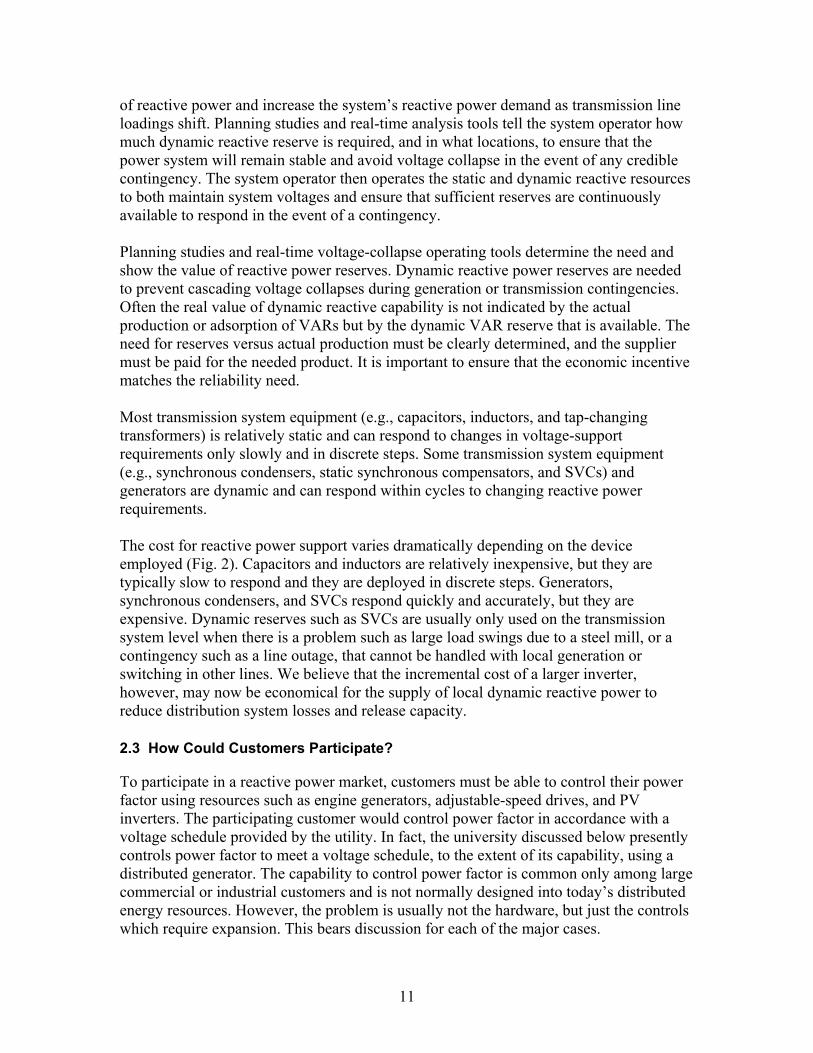
Most transmission system equipment (e.g., capacitors, inductors, and tap-changing transformers) is relatively static and can respond to changes in voltage-support requirements only slowly and in discrete steps. Some transmission system equipment (e.g., synchronous condensers, static synchronous compensators, and SVCs) and generators are dynamic and can respond within cycles to changing reactive power requirements. The cost for reactive power support varies dramatically depending on the device employed (Fig. 2). Capacitors and inductors are relatively inexpensive, but they are typically slow to respond and they are deployed in discrete steps. Generators, synchronous condensers, and SVCs respond quickly and accurately, but they are expensive. Dynamic reserves such as SVCs are usually only used on the transmission system level when there is a problem such as large load swings due to a steel mill, or a contingency such as a line outage, that cannot be handled with local generation or switching in other lines. We believe that the incremental cost of a larger inverter, however, may now be economical for the supply of local dynamic reactive power to reduce distribution system losses and release capacity.

2.3 How Could Customers Participate?

To participate in a reactive power market, customers must be able to control their power factor using resources such as engine generators, adjustable-speed drives, and PV inverters. The participating customer would control power factor in accordance with a voltage schedule provided by the utility. In fact, the university discussed below presently controls power factor to meet a voltage schedule, to the extent of its capability, using a distributed generator. The capability to control power factor is common only among large commercial or industrial customers and is not normally designed into today�’s distributed energy resources. However, the problem is usually not the hardware, but just the controls which require expansion. This bears discussion for each of the major cases.

11

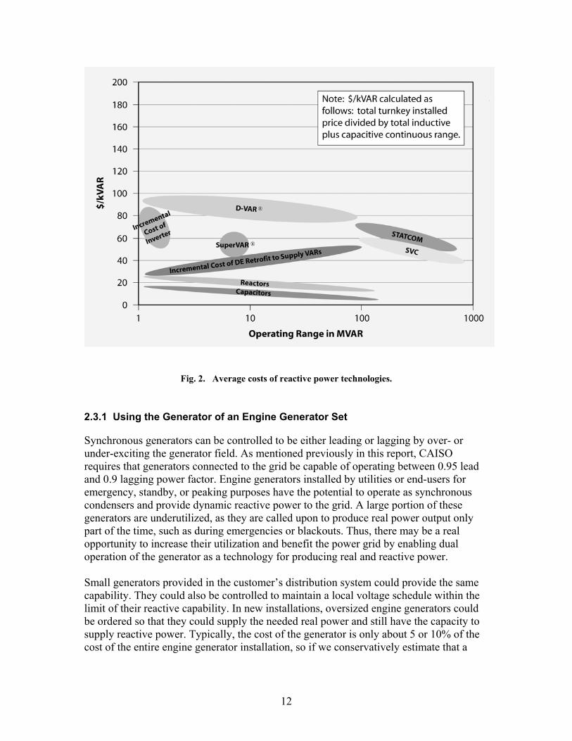
Fig. 2. Average costs of reactive power technologies.

2.3.1 Using the Generator of an Engine Generator Set

Synchronous generators can be controlled to be either leading or lagging by over- or under-exciting the generator field. As mentioned previously in this report, CAISO requires that generators connected to the grid be capable of operating between 0.95 lead and 0.9 lagging power factor. Engine generators installed by utilities or end-users for emergency, standby, or peaking purposes have the potential to operate as synchronous condensers and provide dynamic reactive power to the grid. A large portion of these generators are underutilized, as they are called upon to produce real power output only part of the time, such as during emergencies or blackouts. Thus, there may be a real opportunity to increase their utilization and benefit the power grid by enabling dual operation of the generator as a technology for producing real and reactive power. Small generators provided in the customer�’s distribution system could provide the same capability. They could also be controlled to maintain a local voltage schedule within the limit of their reactive capability. In new installations, oversized engine generators could be ordered so that they could supply the needed real power and still have the capacity to supply reactive power. Typically, the cost of the generator is only about 5 or 10% of the cost of the entire engine generator installation, so if we conservatively estimate that a

12

generator with twice the kVA rating costs twice as much, this would only increase the cost of the total installation by about 5 or 10%. In cases where the engine is not being operated, the generator could still function as a synchronous condenser if it is supplied with a clutch. The generator would simply run as a synchronous motor with no load. There are several companies that make clutches that can be installed between generators and their engines. The clutch operates by completely disengaging the engine and the generator when only reactive power is needed. When active or real power is needed, the clutch engages for electric power generation. When the engine is shut down, the clutch disengages automatically, leaving the generator rotating to supply reactive power for power factor correction and voltage control. Throughout these changing modes, the generator can remain electrically connected to the grid, thus providing a quick response to system demands. One important consideration is that emergency engine generators are typically designed to operate only about two weeks per year. Generators purchased to operate in utility service continuously, 24 hours a day, 365 days a year, may cost twice as much as emergency engine generators of the same power rating, but with a clutch only the generator, not the engine, need be rated for extended service.

2.3.2 Use of an Inverter

Inverters supplied with PV systems, adjustable-speed drives, microturbines, and active power filters can be used to supply reactive power if they are equipped with an �“active front end.�” The active front end is a way to control the inverter so that the power factor drawn by the inverter can be adjusted in real time. Any pulse-width-modulated inverter can theoretically be controlled in this fashion, but modifying the manufacturer�’s existing control programming on an existing inverter would be prohibitively expensive. On the other hand, purchasing the inverter with an active front end may be an economical choice if the customer has the opportunity to provide a voltage regulation service. The cost of an active front end will be discussed in Section 3.

2.3.3 Use of a Stepped Capacitor Bank

The authors believe that a stepped capacitor bank would not be suitable for dynamic local voltage regulation for three reasons:

The voltage level in most distribution circuits moves through transients several times per day, and capacitor switches would soon wear out. Replacing worn out capacitor switches is a major cost of distribution system maintenance today.

Rapid transient response is required. If the transient can be stopped quickly, motor stall may be avoided along with the possibility of a much deeper transient, or even voltage collapse.

The effectiveness of capacitors is reduced with the square of the voltage. When they are needed most, during severe transients, they are least effective.

13

Capacitors located close to loads are the source of problems such as capacitive resonance and switching surges when nonlinear loads or multi-speed motor starters are used.

2.4 Consequences of Inadequate Reactive Reserve

There are two types of consequences from having insufficient reactive reserves, namely reliability consequences and financial consequences, and of course these are closely linked. The reliability consequences of insufficient reserves are fairly well known to be the risk of voltage collapse and blackout. The cost of blackout is severe, and the value of lost load (VoLL) is often approximated at between $5,000 and $10,000 per MWh. To avoid these consequences, system operators procure the needed reactive power by whatever means are necessary. The benefit of dynamic reactive power production from distributed resources is the enhanced grid reliability that these resources will offer in the face of contingencies, as well as the possibility of lowering the procurement cost of the product itself. If the dynamic production of reactive power is instrumental in avoiding a localized or full-scale blackout that would have occurred without these resources, then this is a significant saving, albeit somewhat unquantifiable because it is impossible to measure a phenomenon that has been prevented from occurring. At this point the value to the distributed dynamic reactive power production, by helping to prevent a blackout, far exceeds any cost procurement savings that it might have entailed. If a system operator has insufficient reactive reserves then the system may be characterized by low voltage conditions, made worse by the distribution system siphoning off VARs. Due to the heat wave and associated low voltage conditions experienced in July of 1999 in the PJM Interconnection Regional Transmission Organization (PJM RTO), a review team tasked with determining the root cause stated that �“VARs from the transmission system should not be used to support distribution voltage.�” The root cause was established as �“There was no well defined, common load, power factor criteria or a criteria as to the source of VARs for system energy transfers�” (PJM 2000). The greatest benefit of dynamic VAR production lies in the improved stability of the transmission system. The reason for this is that the amount of reactive power that is available on the system has the effect of influencing/setting path transfer limits, as voltage is one of the three main things that are controlled for: the other two are thermal limits and stability. Thus the benefits of distributed dynamic reactive power seem twofold:

It may decrease the cost of dynamic reactive power at the system level. This cost is passed through to ratepayers.

If voltage control improves (thereby improving reliability), it may be possible to adjust the path transfer limits, which would accommodate more low-cost power to meet load because of decreased congestion and redispatch costs, etc. These savings could be large, certainly much larger than the direct savings.

14

They would further allow more efficient usage of the existing transmission infrastructure. Dynamic reactive power supplied at the load also reduces losses in the distribution system.

The limits on transmission lines are generally set by one of three binding elements: thermal limits, stability limits, and voltage limits; and they typically depend upon the transmission line length, as shown in Fig. 3. In the more integrated eastern interconnection network it is often thermal limits that bind, whereas in the west, with its longer lines and lower energy density, stability limits are often the limiting factor.

Estimating the potential savings from improving the supply of reactive power at the system level is complex to say the least. There are two real sources of savings. If path transfer capabilities are increased with no change in the physical infrastructure, then more cheap power can meet load. A proxy for the size of the �“potential�” savings is the inter-zonal congestion costs on the major branch groups at the CAISO, which may not always be significant. In 2004�–2006 the average inter-zonal congestion cost for the year was $55 million (CAISO 2007, Chapter 5 page 2). Another aspect is the fact that needed transmission capacity is not being built quickly, and in urban areas such as San Francisco, a good case can be made for the use of local dynamic reactive support to increase transmission capacity of the existing lines. If local reactive power in San Francisco obviated the need for an RMR contract, the potential savings would be the added cost of the unit within the load pocket as compared with the cost of a more competitive unit outside the load pocket. Estimating the savings is difficult because of the opacity of much of this accounting; however, a purely hypothetical analysis of an increase in maximum transfer capability as limited by the voltage stability margin is provided in Section 4.1 as an illustration.

0

1000

2000

3000

4000

5000

0 100 200 300 400 500

LINE LENGTH (miles)

LIN

E LO

AD

(M

6000

7000

8000

600

W)

THERMALLIMIT

765 kV500 kV345 kV230 kV

VOLTAGE LIMIT

STABILITY LIMIT

Tline

Fig. 3. Transmission line capacity is limited by thermal capability, voltage support, or stability concerns, depending on the line length.

15

3. Cost of Supply — Customer and Utility Viewpoints

3.1 Estimated Costs for Customers to Supply Reactive Power

Four customers were visited and a brief assessment was made of their potential to supply reactive power. An informal estimate was also made of the cost to the customer for modifications to supply reactive power in accordance with a voltage schedule. The four customers are a shopping center, a conventional generating station (which is s presently supplying reactive power in accordance with a voltage schedule), an urban university campus, and a steel-rolling mill. As expected, these cases show that installing voltage control capability when the customer�’s electrical distribution system is built is considerably less expensive than retrofitting it later. In each case, we examine the possibility of the customer absorbing or supplying reactive power in response to a voltage schedule and estimate the equipment cost as a present value. We add the annual preventive maintenance cost and estimated I2R losses to find the annualized present value of the capacity cost per kVAR.

3.1.1 Shopping Center With Adjustable-Speed Drives with Active Front Ends

Our first example customer is an urban shopping mall with approximately a 2-MW load that normally operates at 0.9 lagging power factor. Let us consider modifications to enable the mall to control its power factor up to a level of 0.95 leading in response to a voltage schedule supplied by the distribution utility. This change of power factor, from 0.9 lagging to 0.95 leading, provides a capability to supply 1.6 megavolt-amperes reactive (MVAR). The mall has approximately 20 air conditioning blower and compressor motors ranging in size from roughly 50 to 70 Hp. These motors have a total coincidental load of about 1 MW. One possible source for dynamic reactive power, and a modification that would also improve the efficiency of the shopping center�’s air conditioning, is to install 20 variable-frequency motor drives with a common rectifier that has an active front end. The active front end enables the rectifier to control the power factor of the power it is drawing. The rectifier would have a rating of 2 MVA and would be capable of supplying or absorbing 1.73 MVAR, which is enough to cover the needed supply capability of 1.6 MVAR. Ten of the variable-frequency drives would be rated at 50 hp and ten at 70 hp. Siemens prepared a cost estimate for this adjustable-speed drive with active front end that includes an isolation transformer, main disconnect, active front end common bus, and 20 motor drive modules (bookshelf motor modules). The estimate totals $450,000 and is attached as Appendix 5. If standard adjustable-speed drives and a transformer were purchased, the cost would be about $185,000. If we assume that standard adjustable-speed drives are justified for a modification to improve efficiency, then the additional cost for the common active front end is about $265,000. If the standard adjustable-speed drives are in an energy saving measure, either as a retrofit or at the time of the shopping center installation, the installation cost of the drives could probably be easily amortized by the energy savings and would not need to be included. Thus we will only consider the additional cost for the active front end.

16

The active front end has a lifetime of about 20 years. We will assume that the maintenance cost is $3000 per year, the interest is 10%, and inflation is 3%. We will also assume that losses due to the reactive current flow are 2% of the MVAR rating and are at one-half the rated kVA for half of the total time, and that the cost of power is $0.1/kWhr. This yields about $14,000 in losses annually. The annualized net present value of providing the reactive power would then be roughly $60,000 for 1.6 MVAR, or $60,000 for 3.2 MVAR if we consider the total inductive plus capacitive range of the active front end. This gives us an estimate of about $19/kVAR capacity cost to provide the dynamic reactive capability at the shopping center if we retrofit the active front end inverter with a common bus into the existing shopping mall. As we will see in later examples, this is a relatively high cost. This example demonstrates the economic need to install the dynamic reactive capability when the adjustable-speed-drive system is installed rather than to retrofit it later.

3.1.2 Conventional Generator

This conventional generator has two gas turbine generators, one of which is normally operating and regulating bus voltage in accordance with a voltage schedule. The generator is not required to sacrifice real power production in order to produce reactive power to support voltage. The generators are run based on market conditions and their bid price for energy. Because the generators are required by contract to be capable of operation from 0.9 lag to 0.95 leading, the only additional cost in operating them through this range is the additional I2R cost and other losses associated with current flow in the generator windings and operation of the exciter. There are various methods for calculating this cost to the generator operator, but a reasonable guess of the upper limit to this cost can be derived from the payments that system operators provide to generators for reactive support. These range from about $1 to $4 for each kVAR of capacity paid annually. Reactive support from large generators is inexpensive, but as discussed earlier, it is often in the wrong place, and does not travel well. In the CAISO reactive support from generators is just considered a cost of doing business and is not charged separately. There are no savings due to distribution system loss reduction. For generators located close to major load centers, we can find savings due to increased transmission capacity. These generators, though, will typically be seeing a higher locational price for energy anyway, and an additional locational payment for reactive power would be impractical. If the CAISO needs to provide reactive support in excess of the D curve, the generator can be paid the lost opportunity cost for the real power output that has to be curtailed.

3.1.3 Steel-Rolling Mill

A single-line diagram of a portion of the rolling mill system is shown in Fig. 4, with the monitoring locations identified. S and C Electric performed an evaluation of reactive power demand for the mill and provided a brief report on potential solutions (Appendix 8). A 20-kV feed from PG&E provides electrical service to the mill. The plant is supplied by two parallel 2500-kVA, 20-kV to 4.16-kV transformers. The 4.16-kV bus on the secondary of the two parallel transformers is where the plant load is connected. Roughly 70% of the total plant load is made up of one 800-hp DC motor and an induction furnace. Some additional motors and drives, as well as miscellaneous loads, are also connected to the 4.16-kV bus.

17

The reactive power flow to the mill was between 900 kVAR and 1650 kVAR. Power factor varied from 0.5 to 0.9 lagging. The real power supplied to the mill varies rapidly from about 1 MW to 2 MW. S and C determined that the power factor could be corrected and made to go to 0.95 leading by using a 2500-kVAR Pure Wave AVC system. The S and C Pure Wave AVC system sizing study is given in Appendix 8. Using the 20-year life of the AVC, the annualized cost would be about $20/kVAR. The cost-recovery analysis is shown in Appendix 7. The AVC uses discrete steps of thyristor switched capacitors to supply reactive compensation on a cycle by cycle basis. The AVC would measure the reactive portion of load current and then match the lagging current by switching in the proper number of capacitor stages. This can be done on a per-phase basis, which would work best for an unbalanced load like the rolling mill.

Fig. 4. Single-line diagram for a steel-rolling mill.

Typically the AVC attempts to exactly match the reactive current and therefore would bring the power factor up to around 1.0. However, the controls can be configured to over compensate the lagging reactive current that is seen flowing to the load, which would

18

result in a leading power factor. Compensating the lagging reactive current also helps to limit the effect the load has on the system voltage by locally providing the necessary VARs. This results in less voltage drop across the system impedance. The AVC would be preferable to slower, conventional switched capacitor banks because it can compensate for faster transients and maintain a more consistent power factor. The AVC can also provide a more refined compensation because it can switch capacitors on in up to 15 discrete steps, allowing for a closer match to the required compensation.

3.1.3 University with PV Inverter with Active Front End

The PV inverter under consideration has a rated output of 0.5 MW, an 0.8 power factor, and 0.625 MVA. We will assume that this inverter has a cost of $543 per kVA by using the Satcon price given in Appendix 6. The additional inverter cost to increase capacity from 1.0 to 0.8 power factor can be based on the additional kVA capacity. At 1.0 power factor, the 500-kW inverter is rated at 500 kVA; at 0.8 power factor, the inverter is rated at 625 kVA. The additional 125 kVA, at a cost of $200/kVA, represents an additional cost of $25,000. If the inverter has the additional kVA capacity, there should be no additional cost for designing the inverter with the control capability to control power factor within its kVA capability. With a power factor of 0.8, the inverter can supply 375 kVAR, both leading and lagging. We calculate the inverter annualized operating cost assuming the inverter has a 20-year life. Typically, utility-grade generation equipment has a 40-year design life, but the manufacturer�’s literature states that the inverter has a 20-year life. If we calculate the annualized capital and operating cost including losses for this additional cost, at a component cost interest of 10%, and inflation of 3%, we find an annualized cost of $4,400 (Appendix 2). Now, we assume that we supply reactive power during the day to boost voltage and absorb it at night to buck voltage. We can utilize both the leading and lagging dynamic reactive capability of the inverter as a service to the distribution company. The 375 kVAR can then be used in both the leading and lagging directions for a total dynamic capability of 750 kVAR. The total incremental cost to the university on an annualized basis for supplying dynamic reactive power is then $6/kVAR. This cost will be compared with benefit in Section 5.

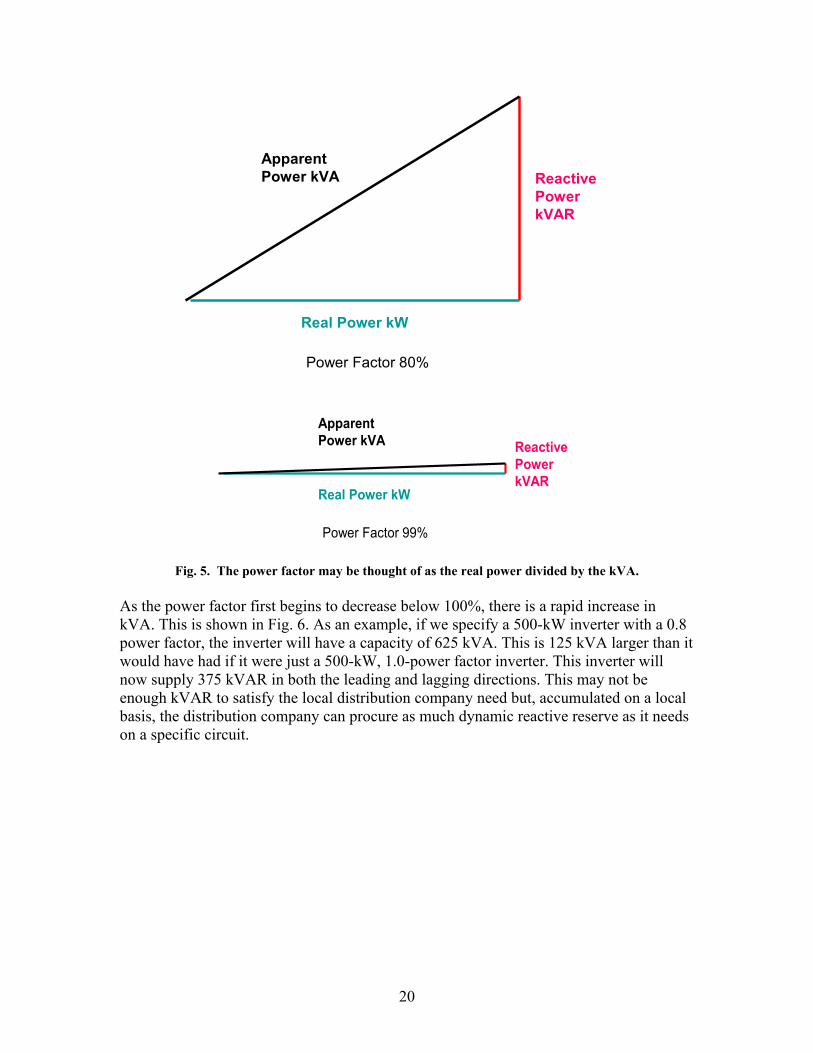
An interesting aspect of specifying the inverter to have a lower power factor than 1.0 is that the cost of the VAR capacity in $/k is quite low when the power factor is first reduced below 1.0, but then extra kVAR available reduces as the power factor is reduced. The kVA is the square root of the sum of the squares of the real and reactive power. The power factor may be thought of as the real power divided by the kVA. In a right triangle, the kVA is the hypotenuse, and the real and reactive power are the other two sides, as shown in the Figure 5.

19

Apparent Power kVA

Real Power kW

Reactive Power kVAR

Power Factor 80%

Apparent Power kVA

Real Power kW

Reactive Power kVAR

Power Factor 99%

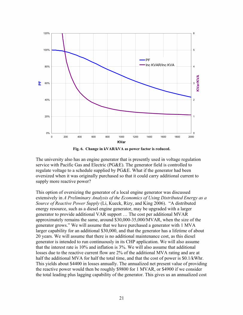
Fig. 5. The power factor may be thought of as the real power divided by the kVA. As the power factor first begins to decrease below 100%, there is a rapid increase in kVA. This is shown in Fig. 6. As an example, if we specify a 500-kW inverter with a 0.8 power factor, the inverter will have a capacity of 625 kVA. This is 125 kVA larger than it would have had if it were just a 500-kW, 1.0-power factor inverter. This inverter will now supply 375 kVAR in both the leading and lagging directions. This may not be enough kVAR to satisfy the local distribution company need but, accumulated on a local basis, the distribution company can procure as much dynamic reactive reserve as it needs on a specific circuit.

20

0%

20%

40%

60%

80%

100%

120%

0 200 400 600 800 1000 1200 1400 1600 1800 2000

KVar

PF

0

1

2

3

4

5

6

KVa

r/KVA

PFInc KVAR/Inc KVA

Fig. 6. Change in kVAR/kVA as power factor is reduced.

The university also has an engine generator that is presently used in voltage regulation service with Pacific Gas and Electric (PG&E). The generator field is controlled to regulate voltage to a schedule supplied by PG&E. What if the generator had been oversized when it was originally purchased so that it could carry additional current to supply more reactive power? This option of oversizing the generator of a local engine generator was discussed extensively in A Preliminary Analysis of the Economics of Using Distributed Energy as a Source of Reactive Power Supply (Li, Kueck, Rizy, and King 2006). �“A distributed energy resource, such as a diesel engine generator, may be upgraded with a larger generator to provide additional VAR support �… The cost per additional MVAR approximately remains the same, around $30,000-35,000/MVAR, when the size of the generator grows.�” We will assume that we have purchased a generator with 1 MVA larger capability for an additional $30,000, and that the generator has a lifetime of about 20 years. We will assume that there is no additional maintenance cost, as this diesel generator is intended to run continuously in its CHP application. We will also assume that the interest rate is 10% and inflation is 3%. We will also assume that additional losses due to the reactive current flow are 2% of the additional MVA rating and are at half the additional MVA for half the total time, and that the cost of power is $0.1/kWhr. This yields about $4400 in losses annually. The annualized net present value of providing the reactive power would then be roughly $9800 for 1 MVAR, or $4900 if we consider the total leading plus lagging capability of the generator. This gives us an annualized cost

21

to the customer of $4.9 per kVAR for supplying reactive power from the generator. This analysis is provided in Appendix 3.

3.2 System Operator Perspective on Cost to Supply Reactive Power

RTOs can use a broad range of incentives. They can still contract with generators on a cost-of-service basis, but more importantly, they can often use market mechanisms as incentives. Although there are currently no jurisdictions in North America that have a market-based incentive system for reactive power, we believe that in the future there will be compensation for dynamic reactive power supplied from distribution customers for voltage control. At this time, the ties from the Pacific Northwest to San Francisco are limited by reactive power flow. If the distribution company could provide a dynamic reactive power service to the RTO, it would have value in reducing congestion in the transmission corridors. As the distribution companies do not operate markets and the sites for the potential supply are at the distribution level rather than at the transmission level, it would make sense for the distribution companies to provide a tariff as an incentive for sites to supply dynamic reactive power, and then act as aggregators. Once the aggregators had sufficient capacity to operate at a power factor of 1.0, it would be possible for the distribution system to provide reactive power to the system operator for monetary gain. In this manner the system operators would reach into the distribution utility and monetize the benefit produced by the tariff structure of that utility. This could occur either via existing procurements based on cost of service, or perhaps via future market mechanisms that allow for both the capacity and production of reactive power to be priced without regard to the technology used to produce it or its source. This all-encompassing market approach would provide clearer economic incentives than a tariff rate and would allow either the aggregators or conceivably the larger customer to directly provide reactive power. As mentioned earlier, the CAISO has a conditions-of-participation model for supplying reactive power at the system level. Generators must supply reactive power in accordance with the voltage schedule if they are to connect. Generating units are not reimbursed for their production of reactive power unless they are required to reduce their real power output, for which they are paid the opportunity cost of the foregone power, which is simply defined as the difference between the market clearing price and the unit bid cost. Most of the payments for reactive power in the CAISO occur via RMR contracts between the CAISO and the unit owners �— often composite contracts that serve a number of different reliability needs �— but the vast majority of them are for voltage support, and all of these costs are assessed back to the participating transmission owner. In 2006 these costs stood at $428 million, compared to $505 million in 2005 (CAISO 2007, Chapter 6, page 12). This adds roughly $2 per MWh to the cost of energy. Clearly not all of these costs are going to disappear, as these generators might well remain the most economical providers of reactive power. However, adding a new class of competition (distributed reactive capacity) could validate costs, and in some circumstances might prove to provide reactive power more cheaply than generators.

22

More recently the number of RMR contracts has declined significantly, and units are instead given RA contracts as part of the CAISO�’s bilateral capacity requirement. Costs in these contracts are much less visible than in RMR contracts.

3.3 Estimate of Cost to the Distribution Utility for Providing Reactive Power

The estimated capital cost for distribution system capacitors is $22,000 for a 5-MVAR capacitor bank (Li, Kueck, Rizy, and King 2006). This study also found that the cost of preventive maintenance for the capacitor bank was $3600 per year. Much of this expense was due to lightning damage, but we use the $3600 figure even though the incidence of lightning is relatively low in California, because this study is intended to be applicable nationally. Interestingly, the local utility that provided the information felt strongly that the capacitors also caused the maintenance on their substation voltage regulator to be $6000 per year because the regulator has to move often to adjust voltage. We have included this cost, because the reactive supply from capacitors should be commensurate with the adjustable supply from inverters and synchronous generators. The capacitor bank has a 10-year service life, and we assume has a 10-year tax life. We assume the tax rate is 35%, inflation is 3%, and the cost of capital is 6%. This gives an annualized payment for the net present value of about $14,000. Divided by 5 MVAR, this gives an annualized net present value, or capacity cost, of $2.8 per kVAR for reactive power supplied from distribution capacitors. This analysis is provided in Appendix 4.

4. Value of Supply – System Operator and Utility Viewpoints

4.1 Value at the Distribution Level, Subtransmission, and Grid

As a first step in estimating the value of voltage support, it would be reasonable to simply average the gross (transmission-level) payments that are presently being used by various transmission system operators around the country. (As mentioned earlier, the cost of supply of reactive power is not �“split out�” by the CAISO; it is rolled into the amount the generators bid for basic energy.) FERC 2005, Table 9, provides the effective gross support rate in $/MVAR-year for 22 locations. The average annualized rate is about $4.5/kVAR. This provides a useful figure for the basic value of voltage support at the transmission level, but we believe that the value of voltage support at the load is significantly higher. At the load, one must also take into consideration the reduction of losses in the distribution system and the increased capacity of the transmission system. We estimate these values using the following examples (Li, Kueck, Rizy, and King 2006).

4.1.1 Example of Reduced Losses Due to Reactive Support at the Load

In the simple system shown in Fig. 7, there is a generation bus, a load bus, and a line connecting the two buses. Here we assume that the load power factor is 0.90, which makes P = 1 MW and Q = 0.484 MVAR numerically. We also assume that the compensation device will inject

23

G

P+jQ Qc

Qc = 0.156 MVAR to make the load power factor 0.95, i.e., P = 1 MW and Q = 0.329 MVAR. Injection of reactive power at the receiving end may raise the voltage and reduce the line current. Since the real power loss is I2R, the loss will be reduced if the current is reduced with the assumption that the load-side voltage remains the same. The actual reduction of power loss is estimated as follows. The original line loss without compensation is

22

22

2

222 235.1484.01

VRR

VR

VQPRIPloss .

The line loss with compensation to unity load power factor is

22

22

2

222 108.1329.01

VRR

VR

VQPRIPloss .

The total saved loss amount will be (1.235 �– 1.108)/1.235 = 10.3% for every 0.156-MVAR compensation to a load pocket of 1MW + j0.484 MVAR. If the total system loss is 3%, the savings in losses will be 1 MW × 3% × 10.3% = 0.00309 MW = 3.09 kW. Although this is not a big number, it can generate considerable savings if it is stretched for a long time period, such as net four months of peak loads when compensation is needed and scaled to a per-MVAR base. Assume the average utility cost for 1 MWh energy is $50/MWh during peak hours, the total savings will be $50 × 0.00309MW × 120 days × 6 peak hours per day = $111/year. The above savings are generated from 0.156-MVAR compensation. Therefore, the savings due to reduced losses are $111 divided by 156 kVAR, or $0.71/kVAR annualized. The utility at the load pocket will benefit from this since it will pay less for system losses.

4.1.2 Increased Line Capacity (Thermal Limit)

If the injection of reactive power lifts a 0.9 lagging power factor at the load side to 0.95 power factor, the line flow will be reduced significantly. This is equivalent to having a

R+jX

Load Pocket

Generation Center

Fig. 7. A simple one-line power system.

24

distribution or transmission line with bigger KVA capacity rating. The saved line capacity may be converted to savings for importing more inexpensive power from this line, compared with dispatching expensive local units in the load pocket. With the sample one-line system at 0.90 power factor, the line flow before compensation is

VVVQP

I 111.1484.01 2222

.

The line flow with compensation to 0.95 power factor is

VVVQP

I 053.1329.01 2222

.

This saves (1.111 �– 1.053)/1.111 = 5.2% of the total capacity of the transmission line, assuming that the voltage remains the same. To capture this savings, we assume the line will reach its limit during the peak hours, i.e., four net months. Therefore, 0.052 MW can be transferred over from generation center to load pocket for every 1-MW load. Assume that the price difference is $5/MWh between the generation center and load pocket. Hence, the total savings for the four peak months will be $5/MWh × 0.052 × 120 days × 6 hours = $187/year. This is the savings from 0.156-MVAR compensation. Therefore, the saving per MVAR-year will be $1200/MVAR-year, or $1.20/kVAR annualized. Typically, the utility at the load pocket will benefit from this since it can purchase cheap power from lower-cost unit.

4.1.3 Increased Maximum Transfer Capability (Stability Limit)

The maximum transfer capability of the sample system is given as

PQkandVEwhere

X2)k1k(EP

22

max .

Again, assume the compensation lifts the power factor from 0.9 to 0.95, or from 1 MW + j0.484 MVAR to 1 MW + j0.329 MVAR, and that the voltage remains the same. It can be easily verified that the maximum transfer capacity has been improved by 15.5%. Therefore, during the four months of peak load, the system may move 15.5% more inexpensive MW from generation center to load center while keeping roughly the same voltage stability margin. Again, this can be converted to a dollar savings amount as $5/MWh × 0.155 × 120 days × 6 peak hours = $558/year. If the compensation is scaled to $/MVAR, it is as significant as $3585/MVAR-year, or $3.58/kVAR annualized. The utility at the load pocket will benefit from this since it can purchase cheap power from lower-cost unit.

25

4.1.4 An Example to Find the Total Economic Benefit of Dynamic Reactive Power Supply in a Hypothetical San Francisco Distribution Circuit

Let us now consider a case study of reactive power benefit using a simulation with parameters estimated to be representative of an urban distribution circuit. First, we calculate the reduced losses in MW due to local reactive power injection in MVAR at the load. The local VAR injection will reduce the current in the system and therefore reduce the real power losses in the network (see Fig. 8). From the last column, the change in loss for a change in reactive power injection can be

summarized as MVarMWPloss /005.0Qc

.

Table 1. Incremental power charge per MVAR

Local VAR Injection (MVAR)

Reduced Ploss (MW)

Incremental Change

(MW / MVar) 0 0 01 0.0050 0.00502 0.0100 0.00503 0.0160 0.00534 0.0190 0.00485 0.0250 0.00506 0.0300 0.00507 0.0350 0.00508 0.0390 0.00499 0.0470 0.0052

10 0.0520 0.0052

26

Reduced Loss vs. Local MVAR Supply

0

0.01

0.02

0.03

0.04

0.05

0.06

0 1 2 3 4 5 6 7 8 9 10

Series1

Fig. 8. Reduced loss vs. local MVAR supply.

4.1.5 Impact to Net Import from PacifiCorp Region

For every 1 MVAR local compensation, it will reduce the local VAR loss within the PG&E transmission system, say x MVAR. Hence, the total net import of reactive power (through the PacifiCorp-PG&E tie line) will be reduced by (1+x) MVAR. Then, the reduced VAR in the tie-line will increase the real power transfer in the same tie-line, because the present limit is the VAR limit. The room left in the tie-line VAR can be then used by MW flow. The simulation verifies this as, shown in Table 2 and Fig. 9.

27

Table 2. Change in power per MVAR

Reduced_Qload (MVar)

Delta Q Import (Mvar)

Delta P Import (MW)

Incremental Change of Delta P per

MVar 0 0.000 0.000 0.000 1 -1.365 0.660 0.660 2 -2.729 1.319 0.660 3 -4.095 1.978 0.659 4 -5.458 2.633 0.658 5 -6.822 3.288 0.658 6 -8.175 3.936 0.656 7 -9.545 4.592 0.656 8 -10.907 5.242 0.655 9 -12.272 5.892 0.655

10 -13.636 6.541 0.654 The third column is calculated using the following equation:

18008.8712000 22linetielinetie QP ,

where is the second column in Table 2; 2000 is the total MVA in the PG&E-PacifiCorp tie-line; 1800 is the total MW import in the tie-line (0.9 power factor assumed); and 871.8 is the total MVAR in the tie-line.

linetieQ

From the last column, it can be summarized that MVarMWQ

P

c

linetie /657.0 .

Inc Import (MW) vs. Local MVAR Supply

0.000

1.000

2.000

3.000

4.000

5.000

6.000

7.000

0 1 2 3 4 5 6 7 8 9 10

Series1

Fig. 9. Incremental import (MW) vs. local MVAR supply.

28

The total economic benefit should be

diffc

linetieEPG

c

loss CQ

PCQP

& ,

where is the cost of PG&E local generation, and is the cost difference between the PG&E local generation and the PacifiCorp imported power.

EPGC & diffC

Taking $50/MW for and $5/MWh for , we have EPGC & diffC

$30,9675)0.65750(0.0058760 /MVar-year, or $30.97/kVAR annualized.

This value must be corrected, however, to account for only 120 peak days per year, and hours per day of peak time: (120 × 6)/8760 is 0.083, which then gives a corrected value of $2.57/kVAR annualized for the total economic benefit.

4.2 Reliability Improvement Due to Local Voltage Regulation

Local voltage regulation to a voltage schedule supplied by the utility can have a very beneficial effect on overall system reliability, reducing the problems caused by voltage dips on distribution circuits such as dimming lights, slowing or stalling motors, dropout of contactors and solenoids, and shrinking television pictures. In past years a voltage drop would inherently reduce load, helping the situation. Light bulbs would dim and motors would slow down with decreasing voltage. Dimmer lights and slower motors typically draw less power, so the situation was in a certain sense self-correcting. With modern loads, this situation is changing. Today many incandescent bulbs are being replaced with compact fluorescent lights that draw constant power as voltage decreases, and motors are being powered with adjustable-speed drives that maintain a constant speed as voltage decreases. In addition, voltage control standards are rather unspecific, and there is a tremendous opportunity for an improvement in efficiency and reliability from better voltage regulation. Capacitors supply reactive power to boost voltage, but their effect is dramatically diminished as voltage dips. Capacitor effectiveness is proportional to the square of the voltage, so at 80% voltage, capacitors are only 64% as effective as they are at normal conditions. As voltage continues to drop, the capacitor effect falls off until voltage collapses. The reactive power supplied by an inverter is dynamic, it can be controlled very rapidly, and it does not drop off with a decrease in voltage. Distribution systems that allow customers to supply dynamic reactive power to regulate voltage could be a tremendous asset to system reliability and efficiency by expanding the margin to voltage collapse.

4.2.1 Effect of Voltage on Motor Torque and Stalling

For the sake of completeness, we will first discuss the effect of motor stall, as a stalled motor presents six times as much electrical load, in general, as a running motor. A major portion of electric load is air conditioning. By some estimates, on a hot day 50% of the

29

total load is from air conditioning. Torque is the rotational force applied by the motor shaft to turn the air conditioning compressor. Air conditioning compressors sometimes require high torques to start. The torque needed to turn the compressor also increases on a hot day. Unfortunately, the torque delivered by an induction motor drops off with the square of the voltage. At 80% voltage, the motor will be delivering 64% of its rated torque. If the motor cannot produce enough torque to turn the compressor, it will stall, or stop turning. Voltages sometimes droop for an instant when there is a fault (short circuit) on the power system. On a hot day, when the system is under heavy load, a fault may pull the voltage down to 75% or lower, and the air conditioning motors may stall. If the motor does not have enough torque to turn the shaft, the motor will stall and continue to draw locked rotor current. The locked rotor current is about six times greater than the normal full load current at a very poor power factor. This additional current flow pulls the voltage down and sometimes causes a micro voltage collapse on just one distribution circuit.

4.2.2 Effect of Motor Stall on Power System Voltage

When the motor is stalled, it is drawing much higher current at a very poor power factor. If many motors are stalled at the same time, the large current flow and poor power factor will cause voltages to droop even further, and possibly collapse. In order to maintain reliability of the electric power system at an acceptable level, risks to voltage stability must be controlled. The loading of major transmission corridors is often limited by stability concerns. Stability is often dominated by the percentage of motor load. The power factor of the load is a dominant factor in voltage collapse. If the power factor can be dynamically corrected using dynamic reactive reserves, the margin to voltage collapse can be expanded without resorting to distribution system upgrades.

4.3 Problematic and Unique Features of Energy Efficient Motors

Unfortunately, new designs of small, energy efficient induction motors may have lower power factors under stalled conditions (Stewart 2005). This lower power factor means that significantly more current is going to flow when the motor is stalled, and that the reactive support must be much higher. The concern with power factor also applies to normal running conditions. DOE has prepared an �“Energy Conservation Standards Rulemaking Framework for Small Electric Motors�” (DOE 2007). This document is to describe the approaches DOE anticipates using to prepare energy conservation standards for small electric motors. On page 13 of this document it states, �“In addition to the internal losses discussed above, small motors with low power factors can induce extra energy losses in the power distribution system that supplies electricity to the motor. These increased currents cause additional losses in the power distribution system.�…�” It is encouraging that this statement is in the framework document for small electric motors. Unfortunately, small electric motors do not lend themselves to efficiency standardization, partially because of their many winding and circuit arrangements, including shaded pole, split phase, capacitor start induction run, capacitor start capacitor run, permanent split

30

capacitor, and others. In addition, the various small motor types have greatly different torque characteristics and power factor for both starting and running. This variability in small motors also applies to air conditioning equipment. There are several techniques for designing a high-efficiency motor, such as designing with a longer core length, deeper and wider slots, larger end rings, and a reduced air gap. Each of these design measures has its drawbacks, one of the most common being a reduction in starting torque, or the ability to turn the compressor shaft. Using larger rotor bars to lower I2R loss in the rotor can reduce stall torque. Increasing magnetic flux density by reducing the effective turns in the stator winding increases inrush current and lowers the power factor.

4.4 Optimum Voltage for Efficient Motor Operation

ANSI Standard C84.1, Voltage Ratings (ANSI 2006) establishes nominal voltage ratings and operating tolerances for 60-Hertz electric power systems above 100 volts. The standard provides a voltage range (A) which will provide satisfactory performance and a secondary range (B) which will provide acceptable performance for a limited duration. The standard specifies that when voltages fall into the secondary range (B), corrective measures shall be undertaken within a reasonable time to improve voltages to meet Range A requirements:

�“When voltages occur outside the limits of Range B, prompt corrective action shall be taken. The urgency of such action will depend upon many factors, such as the location and nature of the load or circuits involved, and the magnitude and duration of the deviation beyond Range B limits.�”

Range B allows voltage to go from 240 down to 208, or 87% of nominal. Unfortunately, this standard is tremendously vague. The authors believe that during a hot afternoon, when the system is under stress, voltages may well be expected to be in Range B for several hours, because prompt corrective action does not have to be taken until the voltage goes beyond the Range B limit (ANSI 2006, page 5). Operating an induction motor at 87% voltage at rated load would typically be thought to result in poor motor efficiency and a greater draw of real power. For example, the IEEE Red Book, Table 3-8, General Effect of Voltage Variations on Induction Motor Characteristics, indicates that typical induction motor efficiency will drop by 3% when voltage is at 90% of nameplate (IEEE 1993). The compelling conclusion here is that existing utility voltage range standards are ambiguous, failing to define the length of time the voltage can be in an abnormal range or go beyond the abnormal range. This lack of specificity in the standard certainly contributes to operational problems both in the power system and in air conditioning. This situation is probably a result of years of capacitor-based voltage control. Today, however, a customer who has a dynamic reactive power supply installed as part of his PV inverter or engine generator can do much better. The utility could easily supply the customer with a voltage schedule to be followed to the extent of his capability, and this would not only improve efficiency, but would also expand the margin to voltage collapse.

31

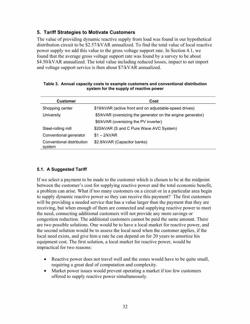
5. Tariff Strategies to Motivate Customers The value of providing dynamic reactive supply from load was found in our hypothetical distribution circuit to be $2.57/kVAR annualized. To find the total value of local reactive power supply we add this value to the gross voltage support rate. In Section 4.1, we found that the average gross voltage support rate was found by a survey to be about $4.50/kVAR annualized. The total value including reduced losses, impact to net import and voltage support service is then about $7/kVAR annualized.

Table 3. Annual capacity costs to example customers and conventional distribution system for the supply of reactive power

Customer Cost

Shopping center $19/kVAR (active front end on adjustable-speed drives) University $5/kVAR (oversizing the generator on the engine generator) $6/kVAR (oversizing the PV inverter) Steel-rolling mill $20/kVAR (S and C Pure Wave AVC System) Conventional generator $1 – 2/kVAR Conventional distribution system

$2.8/kVAR (Capacitor banks)

5.1. A Suggested Tariff

If we select a payment to be made to the customer which is chosen to be at the midpoint between the customer�’s cost for supplying reactive power and the total economic benefit, a problem can arise. What if too many customers on a circuit or in a particular area begin to supply dynamic reactive power so they can receive this payment? The first customers will be providing a needed service that has a value larger than the payment that they are receiving, but when enough of them are connected and supplying reactive power to meet the need, connecting additional customers will not provide any more savings or congestion reduction. The additional customers cannot be paid the same amount. There are two possible solutions. One would be to have a local market for reactive power, and the second solution would be to assess the local need when the customer applies, if the local need exists, and give him a rate he can depend on for 20 years to amortize his equipment cost. The first solution, a local market for reactive power, would be impractical for two reasons:

Reactive power does not travel well and the zones would have to be quite small, requiring a great deal of computation and complexity.

Market power issues would prevent operating a market if too few customers offered to supply reactive power simultaneously.

32

The average small customer probably is not interested in participating in a market, especially if this requires him to reset the power factor control on his PV inverter or the excitation on his generator every day.

The second solution, assessing the local need for reactive supply when the customer applies for connection, and then developing a long-term contract with the customer, could be done with engineering guidelines and would not require expensive engineering analysis on each circuit. If adequate dynamic reactive reserves already exist in an area, more need not be purchased. If dynamic reactive reserves are needed, they can be contracted for at the fixed rate that is known to be economical for the distribution system operator, but which will still be above the cost of supply for the customer, and will help amortize the cost of his PV or CHP system. The total value for local dynamic reactive supply, as found above, is about $7/kVAR on an annualized basis. This includes reduced losses, increased transmission capacity, and increased transfer. (Note that these estimates do not include the value of expanded margin to distribution voltage collapse or power quality. Recently there have been several events of micro voltage collapse from distribution circuits in Southern California Edison. A contracting parallel could be drawn for the distribution system to contract with local sources of dynamic reactive power to provide a margin to distribution voltage collapse. There is a concern that micro voltage collapse events could start to cascade and transform into large-scale events. Assessment of this problem and a recommendation for determining the value of local reactive supply to correct it is beyond the scope of this paper, however.) In some regions, generators are contracted to supply reactive reserves to the transmission system based on their own individual cost of service. It would be too complicated to attempt to contract with every single distributed energy resource based on their cost of providing reactive power. One of the biggest complicating factors is the changing cost of inverters; it is predicted that PV inverter prices are going to drop significantly soon. It would be much better to contract based on a uniform price paid to all distribution company customers. The value of local dynamic reactive supply in our example was about $7/kVAR on an annualized basis. The customer�’s cost in supplying dynamic reactive power ranges from about $5 �– 9/kVAR, annualized. The price that is paid must be reasonable for both the customer and the distribution company. We suggest a figure of $6/kVAR as appropriate compensation. We believe that if such a tariff were put into practice, each distribution company that wished to use it would do a calculation similar to the one above to determine the value of dynamic reactive support in their circuits. Again, as mentioned above, they would only be required to contract for the amount they need in a particular circuit. The customers who can profitably supply dynamic reactive power for this amount would then have a new revenue source to amortize their distributed energy investment. The customer and distribution company would also enjoy improved power quality and tighter voltage regulation �– another benefit we have not attempted to quantify.

33

5.2 The Suggested Tariff Applied to Four Sample Customers

5.2.1 Shopping Center

We found in Section 3.1 the cost of dynamic reactive supply from the shopping center. We considered retrofitting adjustable-speed drives with an active front end, and found the cost to be about $19/kVAR on an annualized basis. Clearly, this modification would not be economical from the sole viewpoint of providing the service of dynamic reactive supply.

5.2.2 University

We found in Section 3. 1. that the total cost to the university on an annualized basis for supplying dynamic reactive power from the new PV inverter, if we consider only the additional cost of oversizing the inverter, is about $6/kVAR on an annualized basis. The annualized cost from an oversized generator is about $5/kVAR. Either of these options look attractive. Most importantly, the PV installation would now have an additional revenue stream of $6 × 750 kVAR, or $4500 per year.

5.2.3 Steel-Rolling Mill

A steel-rolling mill has a power factor that varies from 0.9 to 0.5 lagging. The system which could be used to correct the rapidly fluctuating power factor is a �“Pure Wave�” SVC sold by S and C Electric. The annualized cost of the correction from this system is about $20/kVAR. This modification would not be economical from the viewpoint of providing reactive power, but the compensator would provide improved power quality at the mill, improve distribution system efficiency, and avoid any power factor penalty.

5.2.4 Conventional Generator

The fourth customer was a conventional generator. The plant has two gas turbines with a combined rating of 550 MW. Although not a distribution customer, the conventional generator is included in this report for the sake of completeness. A 200-MW generator is normally operating and connected to the grid. This generator is required to regulate local bus voltage in accordance with a voltage schedule, and this generator responds in about a half cycle. At this time, the generator is not required to go outside of the D curve when performing voltage regulation, so lost opportunity to generate and sell power due to reactive support is not an issue. They operate the generators depending on the market price for energy, and during spring and fall both generators are sometimes shut down. They are also often shut down during the night. They could be ordered to run by the CAISO if reactive reserves were an issue in their area, but this does not normally happen. They are required to meet the voltage schedule as a condition of connection. The costs of exciter operation, generator losses, etc., are quite low, perhaps $1/kVAR or less, and are factored into their bid for energy. Based on a check with this one customer, the market system appears to be working well at the transmission level for reactive reserves and voltage support. At this time, we do not see a need for a special tariff for generator customers connected at the transmission level.

34

6. Conclusion The value of reactive power supplied by the customer has been determined to be about $7/kVAR on an annualized basis. This includes the value of reduced losses, released transmission capacity, and increased transfer capability, as determined using a hypothetical distribution circuit. This does not include the value of increased margin to voltage collapse, because for many utilities voltage collapse is not an issue at this time. In addition, the value of increased margin to voltage collapse is difficult to quantify accurately and is a more subjective measure. The customer�’s cost of providing reactive power ranges from $5 to $20/kVAR on an annualized basis depending on the type of technology used. Thus, at the present time, the range of the cost of supply bounds the value of the service. It would be more desirable, from a profit motive, if the value were about twice, or more, the cost of supply. This would more easily justify procuring distributed energy equipment that could provide the service. In the future, as stress on distribution systems grows and generation capacity dwindles, the importance of efficient operation will grow. In addition, the cost of inverters is predicted to come down. We hope that as the price of supply is reduced, as predicted, and the need grows, that the practice of providing reactive power from microturbines, PV systems, fuel cells, and other inverter-based sources will grow, making them even more economically attractive for the customer.

35

36

7. References

ANSI, 2006. ANSI C84.1-2006, American National Standard for Electric Power Systems and Equipment �– Voltage Ratings (60 Hertz), p. 5.

CAISO, 2007. 2006 Annual Report on Market Issues and Performance, Chapter 5, page 5.2, (http://www.caiso.com/1bb7/1bb77ace17280.pdf).

CAISO, 2007. 2006 Annual Report on Market Issues and Performance, Chapter 6, page 6.12, (http://www.caiso.com/1bb7/1bb77b241b920.pdf).

CAISO, 2008. Tariff, Original Sheet 78 (page 95), http://www.caiso.com/1c0b/1c0ba7d5353c0.pdf.

CAISO, 2008a. See http://www.caiso.com/17c6/17c6f7e55e990.pdf.

CAISO, 2008b. Market Redesign Technology Upgrade, MRTU Tariff 8.2.3.3 http://www.caiso.com/17ba/17ba873e19350.html .

CAISO, 2008c. MRTU Tariff 8.5.6.2.

DOE, 2007. (U.S. Department of Energy, Office of Energy Efficiency and Renewable Energy Building Technologies Program.) Energy Conservation Standards Rulemaking Framework for Small Electric Motors, July 30, 2007.

FERC, 2005. Comments from ISO-NE and NEPOOL Committee to FERC, April 2005, Docket No. AD05-1-000,

Isemonger, A. G., 2007. �“Some Guidelines for Designing Markets in Reactive Power,�” The Electricity Journal, Volume 20, Issue 6, July 2007 pp. 35-45. DOI information: 10.1016/j.tej.2007.06.001.

IEEE, 1993. IEEE Standard 141-1993, IEEE Recommended Practice for Electric Power Distribution for Industrial Plants.

Li, F., J. Kueck, T. Rizy, and T. King, 2006. A Preliminary Analysis of the Economics of Using Distributed Energy as a Source of Reactive Power Supply, Oak Ridge National Laboratory Report ORNL/TM-2006/14, http://www.ornl.gov/sci/decc/Reports/Economics%20of%20DE%20for%20Reactive%20Power%20(ORNL-TM-2006-014).pdf.

PJM, 2000. Results of Heat Wave 1999: July 1999 Low Voltage Condition, Root Cause Analysis, March 21, 2000, Accepted by PJM Operating Committee.

Stewart, V., 2005. Modeling of Stalled Motor Loads for Power System Short Term Voltage Stability Analysis, IEEE Paper No. 0-7803-9156-X/05.

1

Appendixes to A Tariff for Reactive Power

Appendix 1 — Cost Estimate for Oversized Photo Voltaic Inverter Estimates for Inverter Cost ABB - $500k for a 2.5 MVAR Statcom: $200/kVAR, by e mail Ref. 25 ORNL/TM-2006/14 A Preliminary Analysis of the Economics of Using Distributed Energy as a Source of Reactive Power Supply p.12: American Superconductor DVAR is $80 to 100/kVAR p. 40:Cost for additional MVAR capability from an oversized inverter is $56 to 93/kVAR. A Review of PV Inverter Technology Cost and Performance Projections Navigant Consulting Inc. Burlington, Massachusetts Subcontract Report NREL/SR-620-38771 January 2006

Inverter size has an important impact on cost. For instance, a 3kW inverter is about 50% cheaper than a 1 kW unit on a $/kW basis. So, even within a relatively narrow size range, a single average $/kW figure inevitably hides large variations.

Inverter prices for larger installations (> 70 kW) for TEAM-UP were

generally in the $0.40/kW to $0.80/kW price range. (This was clarified by e mail to be 0.4 to 0.8 $/Watt.)

If the basis for current inverter prices is taken as ~$0.65/W, which is

representative of inverters in the 3-6 kW size range (XantrexGT 3.0, SMA SB 6000), then the price forecast for 2020 is $0.38/W, still about 30% higher than the DOE goal.

A price target of around $0.2-0.3/W by 2020 has been set for inverters, which

represents a reduction of 50-75% from current levels. This is most likely to be achieved through increased production volumes and learning-curve improvements.

SatCon PowerGate 500 kW 480/3 Inverter with Combiner http://www.affordable-solar.com/related_1697.htmList Price: $ 286,100.00 Your Price : $ 271,795.00 Product Code : 3040 Description : SatCon PowerGate 500 kW 480/3, AE-500-60-PV-A-G-C Inverter with Combiner PowerGate... SatCon PowerGate 100 kW 480/3, AE-100-60-PV-A-G-C Inverter with Combiner PowerGate inverters offer market-leading reliability, efficiency and ease-of-use for large-scale grid-connected photovoltaic systems. A single enclosure solution, the utility grade PowerGate incorporates a high efficiency transformer and both AC and DC

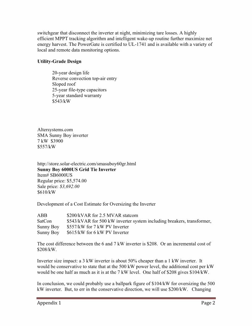
switchgear that disconnect the inverter at night, minimizing tare losses. A highly efficient MPPT tracking algorithm and intelligent wake-up routine further maximize net energy harvest. The PowerGate is certified to UL-1741 and is available with a variety of local and remote data monitoring options. Utility-Grade Design

20-year design life Reverse convection top-air entry Sloped roof 25-year file-type capacitors 5-year standard warranty $543/kW

Altersystems.com SMA Sunny Boy inverter 7 kW $3900 $557/kW http://store.solar-electric.com/smasuboy60gr.html Sunny Boy 6000US Grid Tie Inverter Item# SB6000US Regular price: $5,574.00 Sale price: $3,692.00 $610/kW Development of a Cost Estimate for Oversizing the Inverter ABB $200/kVAR for 2.5 MVAR statcom SatCon $543/kVAR for 500 kW inverter system including breakers, transformer, Sunny Boy $557/kW for 7 kW PV Inverter Sunny Boy $615/kW for 6 kW PV Inverter The cost difference between the 6 and 7 kW inverter is $208. Or an incremental cost of $208/kW. Inverter size impact: a 3 kW inverter is about 50% cheaper than a 1 kW inverter. It would be conservative to state that at the 500 kW power level, the additional cost per kW would be one half as much as it is at the 7 kW level. One half of $208 gives $104/kW. In conclusion, we could probably use a ballpark figure of $104/kW for oversizing the 500 kW inverter. But, to err in the conservative direction, we will use $200/kW. Changing

from a 1.0 to a 0.8 power factor increases the Volt Amp rating by 125 kVA; the original rating is 500 kW, we need 625 kVA. The additional 125 kVA will add $25,000 to the inverter cost.

Appendix 2 — Fixed-Cost-Recovery Analysis for University PV Inverter Additional Cost

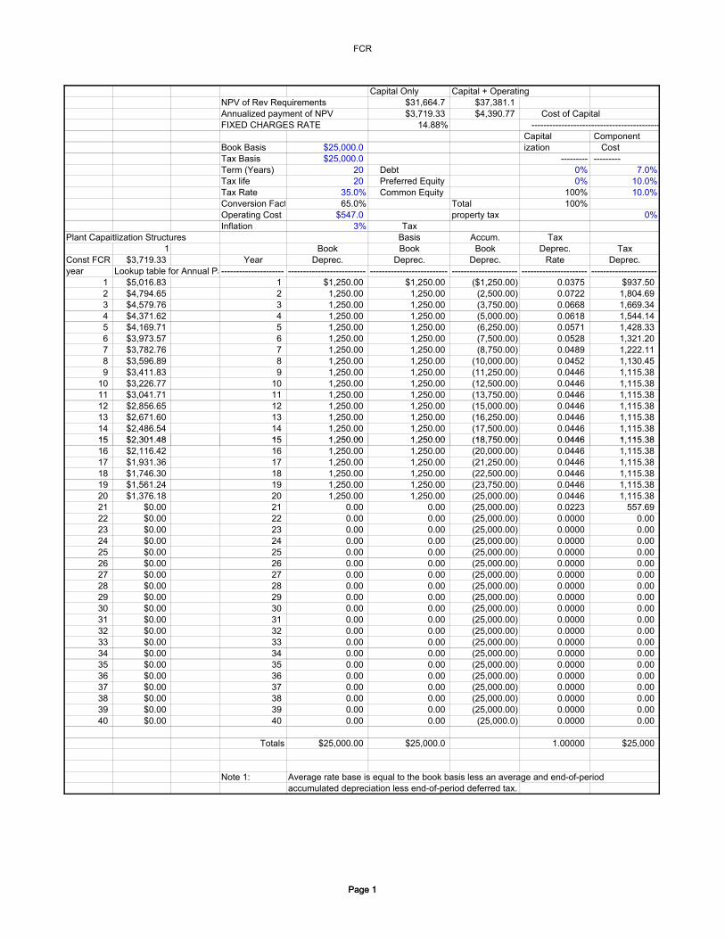
FCR

a

Page 1Page 1

15 $2 301 48 15 1 250 00 1 250 00 (18 750 00) 0 0446 1 115 38

Capital Only Capital + OperatingNPV of Rev Requirements $31,664.7 $37,381.1Annualized payment of NPV $3,719.33 $4,390.77 Cost of CapitalFIXED CHARGES RATE 14.88% -------------------------------------------

Capital ComponentBook Basis $25,000.0 ization CostTax Basis $25,000.0 --------- ---------Term (Years) 20 Debt 0% 7.0%Tax life 20 Preferred Equity 0% 10.0%Tax Rate 35.0% Common Equity 100% 10.0%Conversion Fact 65.0% Total 100%Operating Cost $547.0 property tax 0%Inflation 3% Tax

Plant Capaitlization Structures Basis Accum. Tax1 Book Book Book Deprec. Tax

Const FCR $3,719.33 Year Deprec. Deprec. Deprec. Rate Deprec.year Lookup table for Annual P --------------------- -------------------------- -------------------------- ---------------------- ---------------------- ----------------------

1 $5,016.83 1 $1,250.00 $1,250.00 ($1,250.00) 0.0375 $937.502 $4,794.65 2 1,250.00 1,250.00 (2,500.00) 0.0722 1,804.693 $4,579.76 3 1,250.00 1,250.00 (3,750.00) 0.0668 1,669.344 $4,371.62 4 1,250.00 1,250.00 (5,000.00) 0.0618 1,544.145 $4,169.71 5 1,250.00 1,250.00 (6,250.00) 0.0571 1,428.336 $3,973.57 6 1,250.00 1,250.00 (7,500.00) 0.0528 1,321.207 $3,782.76 7 1,250.00 1,250.00 (8,750.00) 0.0489 1,222.118 $3,596.89 8 1,250.00 1,250.00 (10,000.00) 0.0452 1,130.459 $3,411.83 9 1,250.00 1,250.00 (11,250.00) 0.0446 1,115.38

10 $3,226.77 10 1,250.00 1,250.00 (12,500.00) 0.0446 1,115.3811 $3,041.71 11 1,250.00 1,250.00 (13,750.00) 0.0446 1,115.3812 $2,856.65 12 1,250.00 1,250.00 (15,000.00) 0.0446 1,115.3813 $2,671.60 13 1,250.00 1,250.00 (16,250.00) 0.0446 1,115.3814 $2,486.54 14 1,250.00 1,250.00 (17,500.00) 0.0446 1,115.3815 $2 301 48, . 15 1 250 00, . 1 250 00, . (18 750 00), . 0 0446. 1 115 38, .16 $2,116.42 16 1,250.00 1,250.00 (20,000.00) 0.0446 1,115.3817 $1,931.36 17 1,250.00 1,250.00 (21,250.00) 0.0446 1,115.3818 $1,746.30 18 1,250.00 1,250.00 (22,500.00) 0.0446 1,115.3819 $1,561.24 19 1,250.00 1,250.00 (23,750.00) 0.0446 1,115.3820 $1,376.18 20 1,250.00 1,250.00 (25,000.00) 0.0446 1,115.3821 $0.00 21 0.00 0.00 (25,000.00) 0.0223 557.6922 $0.00 22 0.00 0.00 (25,000.00) 0.0000 0.0023 $0.00 23 0.00 0.00 (25,000.00) 0.0000 0.0024 $0.00 24 0.00 0.00 (25,000.00) 0.0000 0.0025 $0.00 25 0.00 0.00 (25,000.00) 0.0000 0.0026 $0.00 26 0.00 0.00 (25,000.00) 0.0000 0.0027 $0.00 27 0.00 0.00 (25,000.00) 0.0000 0.0028 $0.00 28 0.00 0.00 (25,000.00) 0.0000 0.0029 $0.00 29 0.00 0.00 (25,000.00) 0.0000 0.0030 $0.00 30 0.00 0.00 (25,000.00) 0.0000 0.0031 $0.00 31 0.00 0.00 (25,000.00) 0.0000 0.0032 $0.00 32 0.00 0.00 (25,000.00) 0.0000 0.0033 $0.00 33 0.00 0.00 (25,000.00) 0.0000 0.0034 $0.00 34 0.00 0.00 (25,000.00) 0.0000 0.0035 $0.00 35 0.00 0.00 (25,000.00) 0.0000 0.0036 $0.00 36 0.00 0.00 (25,000.00) 0.0000 0.0037 $0.00 37 0.00 0.00 (25,000.00) 0.0000 0.0038 $0.00 38 0.00 0.00 (25,000.00) 0.0000 0.0039 $0.00 39 0.00 0.00 (25,000.00) 0.0000 0.0040 $0.00 40 0.00 0.00 (25,000.0) 0.0000 0.00

Totals $25,000.00 $25,000.0 1.00000 $25,000

Note 1: Average rate base is equal to the book basis less an average and end-of-periodaccumulated depreciation less end-of-period deferred tax.

FCR

Page 2Page 2

(40 39) 6 834 61 $683 46 368 02 1 250 00 2 301 48 827 39 3 128 86

- Weighted Cost --------

0.00% 1.5 Federal income tax method0.00%

10.00% Tax Depreciation: declining balance, half-year/first-year,10.00% switching to straight-line when greater than declining balance.

Revenue Requirement---------------------- ---------------------- ---------------------- ---------------------- ---------------------- ----------------------

Accum. Average Int + Return Capital TotalDeferred Rate Base +prop tax Inc. Tax Book Revenue Operating Revenue

Tax (Note 1) Require. Require. Deprec. Require. Cost Require.---------------------- ---------------------- ---------------------- ---------------------- ---------------------- ---------------------- ---------------------- ----------------------

$109.38 $24,484.38 $2,448.44 $1,318.39 $1,250.00 $5,016.83 $547.00 $5,563.83(84.77) 23,040.23 $2,304.02 1,240.63 1,250.00 4,794.65 563.41 5,358.06

(231.53) 21,643.47 $2,164.35 1,165.42 1,250.00 4,579.76 580.31 5,160.08(334.48) 20,290.52 $2,029.05 1,092.57 1,250.00 4,371.62 597.72 4,969.34(396.89) 18,978.11 $1,897.81 1,021.90 1,250.00 4,169.71 615.65 4,785.36(421.82) 17,703.18 $1,770.32 953.25 1,250.00 3,973.57 634.12 4,607.69(412.05) 16,462.95 $1,646.29 886.47 1,250.00 3,782.76 653.15 4,435.91(370.21) 15,254.79 $1,525.48 821.41 1,250.00 3,596.89 672.74 4,269.63(323.10) 14,051.90 $1,405.19 756.64 1,250.00 3,411.83 692.92 4,104.75(275.98) 12,849.02 $1,284.90 691.87 1,250.00 3,226.77 713.71 3,940.48(228.86) 11,646.14 $1,164.61 627.10 1,250.00 3,041.71 735.12 3,776.84(181.74) 10,443.26 $1,044.33 562.33 1,250.00 2,856.65 757.18 3,613.83(134.63) 9,240.37 $924.04 497.56 1,250.00 2,671.60 779.89 3,451.49(87.51) 8,037.49 $803.75 432.79 1,250.00 2,486.54 803.29 3,289.82(40 39). 6 834 61, . $683 46. 368 02. 1 250 00, . 2 301 48, . 827 39. 3 128 86, .

6.72 5,631.72 $563.17 303.25 1,250.00 2,116.42 852.21 2,968.6353.84 4,428.84 $442.88 238.48 1,250.00 1,931.36 877.77 2,809.13

100.96 3,225.96 $322.60 173.71 1,250.00 1,746.30 904.11 2,650.41148.07 2,023.07 $202.31 108.93 1,250.00 1,561.24 931.23 2,492.47195.19 820.19 $82.02 44.16 1,250.00 1,376.18 959.17 2,335.35

0.00 0.00 $0.00 0.00 0.00 0.00 0.00 0.000.00 0.00 $0.00 0.00 0.00 0.00 0.00 0.000.00 0.00 $0.00 0.00 0.00 0.00 0.00 0.000.00 0.00 $0.00 0.00 0.00 0.00 0.00 0.000.00 0.00 $0.00 0.00 0.00 0.00 0.00 0.000.00 0.00 $0.00 0.00 0.00 0.00 0.00 0.000.00 0.00 $0.00 0.00 0.00 0.00 0.00 0.000.00 0.00 $0.00 0.00 0.00 0.00 0.00 0.000.00 0.00 $0.00 0.00 0.00 0.00 0.00 0.000.00 0.00 $0.00 0.00 0.00 0.00 0.00 0.000.00 0.00 $0.00 0.00 0.00 0.00 0.00 0.000.00 0.00 $0.00 0.00 0.00 0.00 0.00 0.000.00 0.00 $0.00 0.00 0.00 0.00 0.00 0.000.00 0.00 $0.00 0.00 0.00 0.00 0.00 0.000.00 0.00 $0.00 0.00 0.00 0.00 0.00 0.000.00 0.00 $0.00 0.00 0.00 0.00 0.00 0.000.00 0.00 $0.00 0.00 0.00 0.00 0.00 0.000.00 0.00 $0.00 0.00 0.00 0.00 0.00 0.000.00 0.00 $0.00 0.00 0.00 0.00 0.00 0.000.00 0.00 $0.00 0.00 0.00 0.00 0.00 0.00

$24,709.0 $13,304.86 $25,000 $63,014 $14,698 $77,712

Appendix 3 — Fixed-Cost-Recovery Analysis for University Generator Additional Cost

FCR

a

Page 1Page 1

15 $2 761 77 15 1 500 00 1 500 00 (22 500 00) 0 0446 1 338 46

Capital Only Capital + OperatingNPV of Rev Requirements $37,997.7 $83,770.7Annualized payment of NPV $4,463.19 $9,839.68 Cost of CapitalFIXED CHARGES RATE 14.88% -------------------------------------------

Capital ComponentBook Basis $30,000.0 ization CostTax Basis $30,000.0 --------- ---------Term (Years) 20 Debt 0% 7.0%Tax life 20 Preferred Equity 0% 10.0%Tax Rate 35.0% Common Equity 100% 10.0%Conversion Fact 65.0% Total 100%Operating Cost $4,380.0 property tax 0%Inflation 3% Tax

Plant Capaitlization Structures Basis Accum. Tax1 Book Book Book Deprec. Tax

Const FCR $4,463.19 Year Deprec. Deprec. Deprec. Rate Deprec.year Lookup table for Annual P --------------------- -------------------------- -------------------------- ---------------------- ---------------------- ----------------------

1 $6,020.19 1 $1,500.00 $1,500.00 ($1,500.00) 0.0375 $1,125.002 $5,753.58 2 1,500.00 1,500.00 (3,000.00) 0.0722 2,165.633 $5,495.72 3 1,500.00 1,500.00 (4,500.00) 0.0668 2,003.204 $5,245.94 4 1,500.00 1,500.00 (6,000.00) 0.0618 1,852.965 $5,003.65 5 1,500.00 1,500.00 (7,500.00) 0.0571 1,713.996 $4,768.28 6 1,500.00 1,500.00 (9,000.00) 0.0528 1,585.447 $4,539.31 7 1,500.00 1,500.00 (10,500.00) 0.0489 1,466.538 $4,316.27 8 1,500.00 1,500.00 (12,000.00) 0.0452 1,356.549 $4,094.20 9 1,500.00 1,500.00 (13,500.00) 0.0446 1,338.46

10 $3,872.13 10 1,500.00 1,500.00 (15,000.00) 0.0446 1,338.4611 $3,650.06 11 1,500.00 1,500.00 (16,500.00) 0.0446 1,338.4612 $3,427.99 12 1,500.00 1,500.00 (18,000.00) 0.0446 1,338.4613 $3,205.91 13 1,500.00 1,500.00 (19,500.00) 0.0446 1,338.4614 $2,983.84 14 1,500.00 1,500.00 (21,000.00) 0.0446 1,338.4615 $2 761 77, . 15 1 500 00, . 1 500 00, . (22 500 00), . 0 0446. 1 338 46, .16 $2,539.70 16 1,500.00 1,500.00 (24,000.00) 0.0446 1,338.4617 $2,317.63 17 1,500.00 1,500.00 (25,500.00) 0.0446 1,338.4618 $2,095.56 18 1,500.00 1,500.00 (27,000.00) 0.0446 1,338.4619 $1,873.49 19 1,500.00 1,500.00 (28,500.00) 0.0446 1,338.4620 $1,651.42 20 1,500.00 1,500.00 (30,000.00) 0.0446 1,338.4621 $0.00 21 0.00 0.00 (30,000.00) 0.0223 669.2322 $0.00 22 0.00 0.00 (30,000.00) 0.0000 0.0023 $0.00 23 0.00 0.00 (30,000.00) 0.0000 0.0024 $0.00 24 0.00 0.00 (30,000.00) 0.0000 0.0025 $0.00 25 0.00 0.00 (30,000.00) 0.0000 0.0026 $0.00 26 0.00 0.00 (30,000.00) 0.0000 0.0027 $0.00 27 0.00 0.00 (30,000.00) 0.0000 0.0028 $0.00 28 0.00 0.00 (30,000.00) 0.0000 0.0029 $0.00 29 0.00 0.00 (30,000.00) 0.0000 0.0030 $0.00 30 0.00 0.00 (30,000.00) 0.0000 0.0031 $0.00 31 0.00 0.00 (30,000.00) 0.0000 0.0032 $0.00 32 0.00 0.00 (30,000.00) 0.0000 0.0033 $0.00 33 0.00 0.00 (30,000.00) 0.0000 0.0034 $0.00 34 0.00 0.00 (30,000.00) 0.0000 0.0035 $0.00 35 0.00 0.00 (30,000.00) 0.0000 0.0036 $0.00 36 0.00 0.00 (30,000.00) 0.0000 0.0037 $0.00 37 0.00 0.00 (30,000.00) 0.0000 0.0038 $0.00 38 0.00 0.00 (30,000.00) 0.0000 0.0039 $0.00 39 0.00 0.00 (30,000.00) 0.0000 0.0040 $0.00 40 0.00 0.00 (30,000.0) 0.0000 0.00

Totals $30,000.00 $30,000.0 1.00000 $30,000

Note 1: Average rate base is eqal to the book basis less an average and end of period accumulated d

FCR

Page 2Page 2

(48 47) 8 201 53 $820 15 441 62 1 500 00 2 761 77 6 625 14 9 386 92

e

- Weighted Cost --------

0.00% 1.5 Federal income tax method0.00%

10.00% Tax Depreciation: declining balance, half-year/first-year,10.00% switching to straight-line when greater than declining balance.

Revenue Requirement---------------------- ---------------------- ---------------------- ---------------------- ---------------------- ----------------------

Accum. Average Int + Return Capital TotalDeferred Rate Base +prop tax Inc. Tax Book Revenue Operating Revenue

Tax (Note 1) Require. Require. Deprec. Require. Cost Require.---------------------- ---------------------- ---------------------- ---------------------- ---------------------- ---------------------- ---------------------- ----------------------

$131.25 $29,381.25 $2,938.13 $1,582.07 $1,500.00 $6,020.19 $4,380.00 $10,400.19(101.72) 27,648.28 $2,764.83 1,488.75 1,500.00 5,753.58 4,511.40 10,264.98(277.84) 25,972.16 $2,597.22 1,398.50 1,500.00 5,495.72 4,646.74 10,142.46(401.38) 24,348.62 $2,434.86 1,311.08 1,500.00 5,245.94 4,786.14 10,032.09(476.27) 22,773.73 $2,277.37 1,226.28 1,500.00 5,003.65 4,929.73 9,933.38(506.18) 21,243.82 $2,124.38 1,143.90 1,500.00 4,768.28 5,077.62 9,845.90(494.46) 19,755.54 $1,975.55 1,063.76 1,500.00 4,539.31 5,229.95 9,769.26(444.25) 18,305.75 $1,830.57 985.69 1,500.00 4,316.27 5,386.85 9,703.12(387.71) 16,862.29 $1,686.23 907.97 1,500.00 4,094.20 5,548.45 9,642.65(331.17) 15,418.83 $1,541.88 830.24 1,500.00 3,872.13 5,714.91 9,587.03(274.63) 13,975.37 $1,397.54 752.52 1,500.00 3,650.06 5,886.35 9,536.41(218.09) 12,531.91 $1,253.19 674.79 1,500.00 3,427.99 6,062.94 9,490.93(161.55) 11,088.45 $1,108.84 597.07 1,500.00 3,205.91 6,244.83 9,450.75(105.01) 9,644.99 $964.50 519.35 1,500.00 2,983.84 6,432.18 9,416.02(48 47). 8 201 53, . $820 15. 441 62. 1 500 00, . 2 761 77, . 6 625 14, . 9 386 92, .

8.07 6,758.07 $675.81 363.90 1,500.00 2,539.70 6,823.90 9,363.6064.61 5,314.61 $531.46 286.17 1,500.00 2,317.63 7,028.61 9,346.25

121.15 3,871.15 $387.11 208.45 1,500.00 2,095.56 7,239.47 9,335.03177.69 2,427.69 $242.77 130.72 1,500.00 1,873.49 7,456.66 9,330.15234.23 984.23 $98.42 53.00 1,500.00 1,651.42 7,680.36 9,331.78

0.00 0.00 $0.00 0.00 0.00 0.00 0.00 0.000.00 0.00 $0.00 0.00 0.00 0.00 0.00 0.000.00 0.00 $0.00 0.00 0.00 0.00 0.00 0.000.00 0.00 $0.00 0.00 0.00 0.00 0.00 0.000.00 0.00 $0.00 0.00 0.00 0.00 0.00 0.000.00 0.00 $0.00 0.00 0.00 0.00 0.00 0.000.00 0.00 $0.00 0.00 0.00 0.00 0.00 0.000.00 0.00 $0.00 0.00 0.00 0.00 0.00 0.000.00 0.00 $0.00 0.00 0.00 0.00 0.00 0.000.00 0.00 $0.00 0.00 0.00 0.00 0.00 0.000.00 0.00 $0.00 0.00 0.00 0.00 0.00 0.000.00 0.00 $0.00 0.00 0.00 0.00 0.00 0.000.00 0.00 $0.00 0.00 0.00 0.00 0.00 0.000.00 0.00 $0.00 0.00 0.00 0.00 0.00 0.000.00 0.00 $0.00 0.00 0.00 0.00 0.00 0.000.00 0.00 $0.00 0.00 0.00 0.00 0.00 0.000.00 0.00 $0.00 0.00 0.00 0.00 0.00 0.000.00 0.00 $0.00 0.00 0.00 0.00 0.00 0.000.00 0.00 $0.00 0.00 0.00 0.00 0.00 0.000.00 0.00 $0.00 0.00 0.00 0.00 0.00 0.00

$29,650.8 $15,965.83 $30,000 $75,617 $117,692 $193,309

preciation less end of period deferred tax.

Appendix 4 — Fixed-Cost-Recovery Analysis for Capacitor Banks

FCR

a

Page 1Page 1

Capital Only Capital + OperatingNPV of Rev Requirements $23,468.8 $48,818.9Annualized payment of NPV $3,737.78 $7,775.20 Cost of CapitalFIXED CHARGES RATE 16.99% -------------------------------------------

Capital ComponentBook Basis $22,000.0 ization CostTax Basis $22,000.0 --------- ---------Term (Years) 10 Debt 50% 7.0%Tax life 10 Preferred Equity 0% 10.0%Tax Rate 35.0% Common Equity 50% 12.0%Conversion Fact 65.0% Total 100%Operating Cost $3,600.0 property tax 0%Inflation 3% Tax

Plant Capaitlization Structures Basis Accum. Tax1 Book Book Book Deprec. Tax

Const FCR $3,737.78 Year Deprec. Deprec. Deprec. Rate Deprec.year Lookup table for Annual P --------------------- -------------------------- -------------------------- ---------------------- ---------------------- ----------------------

1 $4,860.73 1 $2,200.00 $2,200.00 ($2,200.00) 0.1000 $2,200.002 $4,502.23 2 2,200.00 2,200.00 (4,400.00) 0.1800 3,960.003 $4,179.02 3 2,200.00 2,200.00 (6,600.00) 0.1440 3,168.004 $3,884.05 4 2,200.00 2,200.00 (8,800.00) 0.1152 2,534.405 $3,611.65 5 2,200.00 2,200.00 (11,000.00) 0.0922 2,027.526 $3,357.33 6 2,200.00 2,200.00 (13,200.00) 0.0737 1,622.027 $3,111.04 7 2,200.00 2,200.00 (15,400.00) 0.0655 1,441.798 $2,864.75 8 2,200.00 2,200.00 (17,600.00) 0.0655 1,441.799 $2,618.45 9 2,200.00 2,200.00 (19,800.00) 0.0655 1,441.79

10 $2,372.16 10 2,200.00 2,200.00 (22,000.00) 0.0655 1,441.7911 $0.00 11 0.00 0.00 (22,000.00) 0.0328 720.9012 $0.00 12 0.00 0.00 (22,000.00) 0.0000 0.0013 $0.00 13 0.00 0.00 (22,000.00) 0.0000 0.0014 $0.00 14 0.00 0.00 (22,000.00) 0.0000 0.0015 $0.00 15 0.00 0.00 (22,000.00) 0.0000 0.0016 $0.00 16 0.00 0.00 (22,000.00) 0.0000 0.0017 $0.00 17 0.00 0.00 (22,000.00)( ) 0.0000 0.0018 $0.00 18 0.00 0.00 (22,000.00) 0.0000 0.0019 $0.00 19 0.00 0.00 (22,000.00) 0.0000 0.0020 $0.00 20 0.00 0.00 (22,000.00) 0.0000 0.0021 $0.00 21 0.00 0.00 (22,000.00) 0.0000 0.0022 $0.00 22 0.00 0.00 (22,000.00) 0.0000 0.0023 $0.00 23 0.00 0.00 (22,000.00) 0.0000 0.0024 $0.00 24 0.00 0.00 (22,000.00) 0.0000 0.0025 $0.00 25 0.00 0.00 (22,000.00) 0.0000 0.0026 $0.00 26 0.00 0.00 (22,000.00) 0.0000 0.0027 $0.00 27 0.00 0.00 (22,000.00) 0.0000 0.0028 $0.00 28 0.00 0.00 (22,000.00) 0.0000 0.0029 $0.00 29 0.00 0.00 (22,000.00) 0.0000 0.0030 $0.00 30 0.00 0.00 (22,000.00) 0.0000 0.0031 $0.00 31 0.00 0.00 (22,000.00) 0.0000 0.0032 $0.00 32 0.00 0.00 (22,000.00) 0.0000 0.0033 $0.00 33 0.00 0.00 (22,000.00) 0.0000 0.0034 $0.00 34 0.00 0.00 (22,000.00) 0.0000 0.0035 $0.00 35 0.00 0.00 (22,000.00) 0.0000 0.0036 $0.00 36 0.00 0.00 (22,000.00) 0.0000 0.0037 $0.00 37 0.00 0.00 (22,000.00) 0.0000 0.0038 $0.00 38 0.00 0.00 (22,000.00) 0.0000 0.0039 $0.00 39 0.00 0.00 (22,000.00) 0.0000 0.0040 $0.00 40 0.00 0.00 (22,000.0) 0.0000 0.00

Totals $22,000.00 $22,000.0 1.00000 $22,000

Note 1: Average rate base is eqal to the book basis less an average and end of period accumulated de

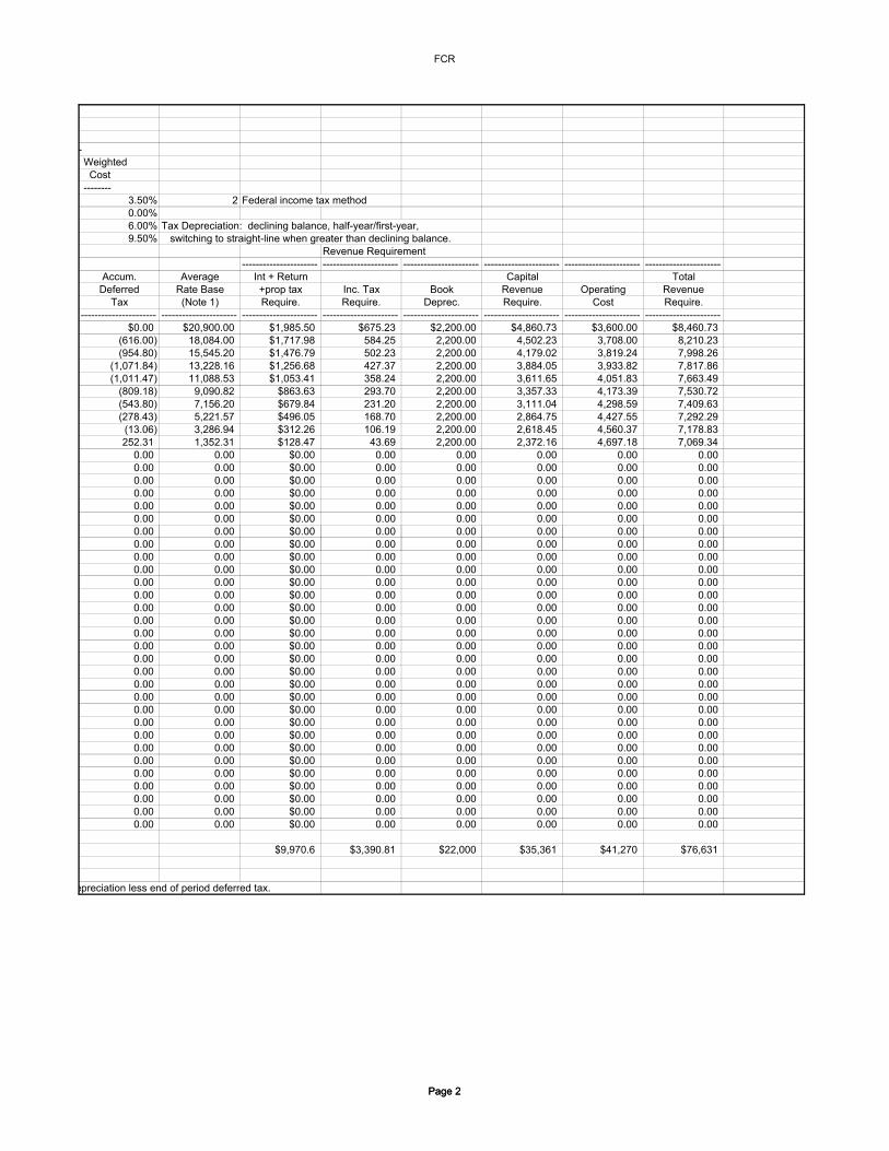
FCR

-

Page 2Page 2

e

Weighted Cost --------

3.50% 2 Federal income tax method0.00%6.00% Tax Depreciation: declining balance, half-year/first-year,9.50% switching to straight-line when greater than declining balance.

Revenue Requirement---------------------- ---------------------- ---------------------- ---------------------- ---------------------- ----------------------

Accum. Average Int + Return Capital TotalDeferred Rate Base +prop tax Inc. Tax Book Revenue Operating Revenue

Tax (Note 1) Require. Require. Deprec. Require. Cost Require.---------------------- ---------------------- ---------------------- ---------------------- ---------------------- ---------------------- ---------------------- ----------------------

$0.00 $20,900.00 $1,985.50 $675.23 $2,200.00 $4,860.73 $3,600.00 $8,460.73(616.00) 18,084.00 $1,717.98 584.25 2,200.00 4,502.23 3,708.00 8,210.23(954.80) 15,545.20 $1,476.79 502.23 2,200.00 4,179.02 3,819.24 7,998.26

(1,071.84) 13,228.16 $1,256.68 427.37 2,200.00 3,884.05 3,933.82 7,817.86(1,011.47) 11,088.53 $1,053.41 358.24 2,200.00 3,611.65 4,051.83 7,663.49

(809.18) 9,090.82 $863.63 293.70 2,200.00 3,357.33 4,173.39 7,530.72(543.80) 7,156.20 $679.84 231.20 2,200.00 3,111.04 4,298.59 7,409.63(278.43) 5,221.57 $496.05 168.70 2,200.00 2,864.75 4,427.55 7,292.29

(13.06) 3,286.94 $312.26 106.19 2,200.00 2,618.45 4,560.37 7,178.83252.31 1,352.31 $128.47 43.69 2,200.00 2,372.16 4,697.18 7,069.34

0.00 0.00 $0.00 0.00 0.00 0.00 0.00 0.000.00 0.00 $0.00 0.00 0.00 0.00 0.00 0.000.00 0.00 $0.00 0.00 0.00 0.00 0.00 0.000.00 0.00 $0.00 0.00 0.00 0.00 0.00 0.000.00 0.00 $0.00 0.00 0.00 0.00 0.00 0.000.00 0.00 $0.00 0.00 0.00 0.00 0.00 0.000.00 0.00 $0.00 0.00 0.00 0.00 0.00 0.000.00 0.00 $0.00 0.00 0.00 0.00 0.00 0.000.00 0.00 $0.00 0.00 0.00 0.00 0.00 0.000.00 0.00 $0.00 0.00 0.00 0.00 0.00 0.000.00 0.00 $0.00 0.00 0.00 0.00 0.00 0.000.00 0.00 $0.00 0.00 0.00 0.00 0.00 0.000.00 0.00 $0.00 0.00 0.00 0.00 0.00 0.000.00 0.00 $0.00 0.00 0.00 0.00 0.00 0.000.00 0.00 $0.00 0.00 0.00 0.00 0.00 0.000.00 0.00 $0.00 0.00 0.00 0.00 0.00 0.000.00 0.00 $0.00 0.00 0.00 0.00 0.00 0.000.00 0.00 $0.00 0.00 0.00 0.00 0.00 0.000.00 0.00 $0.00 0.00 0.00 0.00 0.00 0.000.00 0.00 $0.00 0.00 0.00 0.00 0.00 0.000.00 0.00 $0.00 0.00 0.00 0.00 0.00 0.000.00 0.00 $0.00 0.00 0.00 0.00 0.00 0.000.00 0.00 $0.00 0.00 0.00 0.00 0.00 0.000.00 0.00 $0.00 0.00 0.00 0.00 0.00 0.000.00 0.00 $0.00 0.00 0.00 0.00 0.00 0.000.00 0.00 $0.00 0.00 0.00 0.00 0.00 0.000.00 0.00 $0.00 0.00 0.00 0.00 0.00 0.000.00 0.00 $0.00 0.00 0.00 0.00 0.00 0.000.00 0.00 $0.00 0.00 0.00 0.00 0.00 0.000.00 0.00 $0.00 0.00 0.00 0.00 0.00 0.00

$9,970.6 $3,390.81 $22,000 $35,361 $41,270 $76,631

preciation less end of period deferred tax.

Appendix 5 — Siemens Budgetary Estimate for Adjustable-Speed Drives with Common Active Front End

Siemens Energy & Automation, Inc. Page 1 of 8 Power Conversion Division 100 Technology Drives Tel: (770) 740-3000 Alpharetta, GA 30005 Fax: (770) 740-3050

July 20, 2007

To: Oak Ridge National Laboratory Attn: John D. Kueck Subject: SINAMICS Budgetary Drive System

SE&A, Inc. - PCD, Proposal # AC-07152, Rev. 0 Siemens Energy & Automation, Inc. is pleased to present this budgetary quotation and technical proposal for SINAMICS variable frequency drives. This proposal covers Item 1 from your �“Budgetary Estimate Request�” document. Item 2 is being reviewed by a different Siemens Energy and Automation Group and would come on a different proposal. Item 3 is the active filters for you DC drives, is something we don�’t offer. We attached your original budgetary estimate request for your convenience. Siemens Energy & Automation is also offering an alternative approach to the common bus. In this case we supplied 10 individual active front end drives which could feed two motors per drive. This is referred to as Option #1. Please see the attached documents for our terms and conditions. As one of the world's largest electrical companies, Siemens provides a global experience base in industrial drive solutions. Thank you for the opportunity to present this technical solution to enhance your company's operations. We trust that our technical proposal and prices are of interest and meet your requirements. If you have any questions or require further information, please contact Chuck Fernandez at +1 (770) 740-3549. Sincerely yours, Chuck Fernandez Proposal and Application Engineering Industrial Drives Enclosures: Standard Terms and Conditions of Sale (TC of Sale-SEA-REV 10-1-2004.pdf) Field Service Rates (AD_Service_Rates_2006_Rev 5_1 (01-2007).pdf) Your Budgetary Estimate Request (Budgetary Estimate.2.doc)

cc: Wolfgang Hilmer, Siemens Energy & Automation, Inc.

Appndx5SiemensLetter Page 2 of 8

The following commercial conditions form an integral part of this quotation:

Commercial Conditions 1.0 Price Basis

The budgetary prices are based upon Siemens interpretation of your Inquiry, subject to final clarification and mutual agreement upon the scope of supply. The prices are budgetary in US $ based on the equipment described in this proposal. The variable frequency drive will be shipped FOB U.S. manufacturing facility, Alpharetta, GA, domestic packaging, no freight allowed per the attached terms and conditions.

2.0 Validity This quotation is budgetary and is subject to reconfirmation or change before an order would be accepted. This proposal is subject to credit approval and applicable US government regulations. This quotation is also subject to the customer obtaining any licenses or approvals, which may be required by the appropriate authorities.

3.0 Payment Conditions Project prices are based upon the following payment terms: 20% of the Contract price, to be paid upon receipt of order 80% of the Contract price upon pro rata shipment, or upon notification of readiness for shipment should shipment be delayed for reasons not attributable to Seller All payments are due 30 days after date of invoice. If necessary, it is assumed that payment guarantees or securities acceptable to Siemens will be provided, such as an irrevocable and confirmed letter of credit. The Purchaser shall bear all associated costs for such guarantees or securities. All bonds or guarantees, which might have to be provided by Siemens, are company guarantees. If external bonds or guarantees are required, all associated costs shall be borne by the Purchaser.

4.0 Shipment Period The exact shipment period will be determined at a later date.

5.0 Taxes and Duties The Prices do not include taxes and duties which may become payable under the country of import law. The purchaser shall bear the total cost of all taxes and duties, and if Seller or its employees shall be required to pay for taxes or duties, the Purchaser shall immediately reimburse the Seller.

Appndx5SiemensLetter Page 3 of 8

6.0 Other Conditions For all other commercial terms and conditions, the following attached Terms and Conditions shall apply: "Standard Terms and Conditions of Sale". Please see section 9.0 for additional comments, terms and exceptions.

7.0 Variable Frequency Drive Price Schedule

THE FOLLOWING EQUIPMENT WILL BE BUILT PER IEC STANDARDS

Item QTY Description Unit Price NET Total 1

Base Option

1 S120CM System

This includes an Isolation Transformer, Main Disconnect, Active Front End Common Bus with 20 Motor Modules.

Please refer to Scope of Supply section for more details.

$450,861.00

$450,861.00

1

Option #1

10 S150 Active Front End Variable Frequency Drives

This includes one Isolation Transformer and ten 110 KW Active Front End Drives with Fused Disconnect. Each drive would power two motors.

Please refer to Scope of Supply section for more details.

$35,654.00

$356,540.00

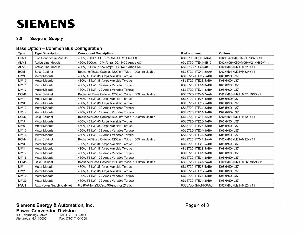
Siemens Energy & Automation, Inc. Page 4 of 8 Power Conversion Division 100 Technology Drives Tel: (770) 740-3000 Alpharetta, GA 30005 Fax: (770) 740-3050

8.0 Scope of Supply Base Option �– Common Bus Configuration

Type Type Description Component Description Part numbers Options LCM1 Line Connection Module 480V, 2500 A. FOR PARALLEL MODULES 6SL3700-0LE42-5BA0 D02+L42+M06+M21+M85+Y11 ALM1 Active Line Module 480V, 900kW, 1574 Amps DC, 1405 Amps AC 6SL3730-7TE41-4B_0 D02+K08+K90+M06+M21+M82+Y11 ALM2 Active Line Module 480V, 900kW, 1574 Amps DC, 1405 Amps AC 6SL3730-7TE41-4B_0 D02+M06+M21+M82+Y11 BCM1 Base Cabinet Bookshelf Base Cabinet 1200mm Wide; 1000mm Usable 6SL3720-1TX41-2AA0 D02+M06+M21+M82+Y11 MM9 Motor Module 480V, 46 kW, 85 Amps Variable Torque 6SL3720-1TE28-5AB0 K08+K90+L37 MM10 Motor Module 480V, 46 kW, 85 Amps Variable Torque 6SL3720-1TE28-5AB0 K08+K90+L37 MM11 Motor Module 480V, 71 kW, 132 Amps Variable Torque 6SL3720-1TE31-3AB0 K08+K90+L37 MM12 Motor Module 480V, 71 kW, 132 Amps Variable Torque 6SL3720-1TE31-3AB0 K08+K90+L37 BCM2 Base Cabinet Bookshelf Base Cabinet 1200mm Wide; 1000mm Usable 6SL3720-1TX41-2AA0 D02+M06+M21+M27+M82+Y11 MM7 Motor Module 480V, 46 kW, 85 Amps Variable Torque 6SL3720-1TE28-5AB0 K08+K90+L37 MM8 Motor Module 480V, 46 kW, 85 Amps Variable Torque 6SL3720-1TE28-5AB0 K08+K90+L37 MM13 Motor Module 480V, 71 kW, 132 Amps Variable Torque 6SL3720-1TE31-3AB0 K08+K90+L37 MM14 Motor Module 480V, 71 kW, 132 Amps Variable Torque 6SL3720-1TE31-3AB0 K08+K90+L37 BCM3 Base Cabinet Bookshelf Base Cabinet 1200mm Wide; 1000mm Usable 6SL3720-1TX41-2AA0 D02+M06+M21+M82+Y11 MM5 Motor Module 480V, 46 kW, 85 Amps Variable Torque 6SL3720-1TE28-5AB0 K08+K90+L37 MM6 Motor Module 480V, 46 kW, 85 Amps Variable Torque 6SL3720-1TE28-5AB0 K08+K90+L37 MM15 Motor Module 480V, 71 kW, 132 Amps Variable Torque 6SL3720-1TE31-3AB0 K08+K90+L37 MM16 Motor Module 480V, 71 kW, 132 Amps Variable Torque 6SL3720-1TE31-3AB0 K08+K90+L37 BCM4 Base Cabinet Bookshelf Base Cabinet 1200mm Wide; 1000mm Usable 6SL3720-1TX41-2AA0 D02+M06+M21+M82+Y11 MM3 Motor Module 480V, 46 kW, 85 Amps Variable Torque 6SL3720-1TE28-5AB0 K08+K90+L37 MM4 Motor Module 480V, 46 kW, 85 Amps Variable Torque 6SL3720-1TE28-5AB0 K08+K90+L37 MM17 Motor Module 480V, 71 kW, 132 Amps Variable Torque 6SL3720-1TE31-3AB0 K08+K90+L37 MM18 Motor Module 480V, 71 kW, 132 Amps Variable Torque 6SL3720-1TE31-3AB0 K08+K90+L37 BCM5 Base Cabinet Bookshelf Base Cabinet 1200mm Wide; 1000mm Usable 6SL3720-1TX41-2AA0 D02+M06+M21+M26+M82+Y11 MM1 Motor Module 480V, 46 kW, 85 Amps Variable Torque 6SL3720-1TE28-5AB0 K08+K90+L37 MM2 Motor Module 480V, 46 kW, 85 Amps Variable Torque 6SL3720-1TE28-5AB0 K08+K90+L37 MM19 Motor Module 480V, 71 kW, 132 Amps Variable Torque 6SL3720-1TE31-3AB0 K08+K90+L37 MM20 Motor Module 480V, 71 kW, 132 Amps Variable Torque 6SL3720-1TE31-3AB0 K08+K90+L37 PSU1 Aux. Power Supply Cabinet 6.3 KVA for 230Vac, 40Amps for 24Vdc 6SL3700-0MX16-3AA0 D02+M06+M21+M82+Y11

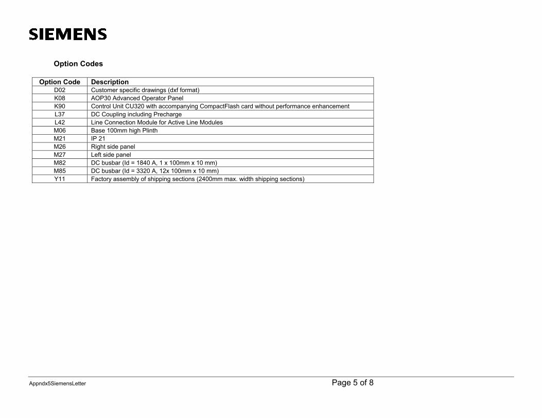
Appndx5SiemensLetter Page 5 of 8

Option Codes

Option Code Description D02 Customer specific drawings (dxf format) K08 AOP30 Advanced Operator Panel K90 Control Unit CU320 with accompanying CompactFlash card without performance enhancement L37 DC Coupling including Precharge L42 Line Connection Module for Active Line Modules M06 Base 100mm high Plinth M21 IP 21 M26 Right side panel M27 Left side panel M82 DC busbar (Id = 1840 A, 1 x 100mm x 10 mm) M85 DC busbar (Id = 3320 A, 12x 100mm x 10 mm) Y11 Factory assembly of shipping sections (2400mm max. width shipping sections)

Siemens Energy & Automation, Inc. Page 6 of 8 Power Conversion Division 100 Technology Drives Tel: (770) 740-3000 Alpharetta, GA 30005 Fax: (770) 740-3050

Line Connection Module (LCM)

Active Line Modules (ALM)AC

DC

AUX. POWER SUPPLIES

AUX. VOLTAGE BUS BARS

Auxillary Power Supply Module (PSU)

Bookshelf Motor Modules (MM)

DCAC

Motor

Compressor #1 480V, 70HP

MM11

DCAC

Motor

Fan #10480V, 50HP

MM10

DCAC

Motor

Fan #1480V, 50HP

MM1

DCAC

Motor

Compressor #10480V, 70HP

MM20

ACDC

4160V Primary

460V Secondary

Base Option �– Common Bus4160V Supply by Others

Appndx5SiemensLetter Page 7 of 8

Sinamics S150

AFE

DCAC

Motor

Fan #2480V, 50HP

MM

ACDC PO

WER

4160V Primary

460V Secondary

Option #1

4160V Supply by Others

Motor

Fan #1480V, 50HP

Sinamics S150

AFE

DCAC

Motor

Fan #10480V, 50HP

MM

ACDC PO

WER

Motor

Fan #9480V, 50HP

Sinamics S150

AFE

DCAC

Motor

Compressor #2480V, 70HP

MM

ACDC PO

WER

Motor

Compressor #1480V, 70HP

Sinamics S150

AFE

DCAC

Motor

MM

ACDC PO

WER

Motor

Compressor #10480V, 70HP

Compressor #9480V, 70HP

Siemens Energy & Automation, Inc. Page 8 of 8 Power Conversion Division 100 Technology Drives Tel: (770) 740-3000 Alpharetta, GA 30005 Fax: (770) 740-3050

9.0 Comments and Exceptions Note: This proposal is not based on a written customer specification. This quote letter and the attachments define Siemens�’ scope of supply and the terms and conditions of sale. Siemens reserves the right to revise this proposal if a specification or additional requirements are received at a later date. Comments: 1. The equipment will be delivered to Oak Ridge National Laboratory in shipping sections with a

maximum width of 2400mm. The exact details concerning the make-up of the shipping sections will be determined at a later date.

2. This proposal does not include labor for additional testing outside of the standard testing performed by Siemens AG.

3. This proposal does not include labor for the assembly of the shipping sections once they are received by Oak Ridge National Laboratory.

4. Drawings will be limited to the DXF format drawings supplied by Siemens AG 5. The ratings and options selected are based on our best interpretation of the requirements of this

application but it is left up to Oak Ridge National Laboratory to verify all ratings, features, options, etc.

6. Additional options or other changes to the scope of supply as quoted will result in additional charges.

7. All Variable Frequency Drives quoted are built to IEC Standards. 8. The IP21 drives in this proposal have been sized based on a 40° C Ambient. This proposal excludes supply of the following items:

Installation design, construction engineering, installation material, cable and installation labor Application specific programming and set-up of the drive systems (may be provided based on

attached field service hourly rate sheet). Field services (start-up, training, etc.) �– (may be provided based on attached field service

hourly rate sheet). Spare parts Assembly labor for the assembly of the shipping sections once shipped from Siemens AG Test labor (outside of standard testing performed by Siemens AG) Training (may be provided based on attached field service hourly rate sheet) Load reactors for motors (only required if cable length requirements are not satisfied �– 300

Meters maximum).

Appendix 6 — SatCon 500-kW Inverter and Switchgear Price Sheet from Affordable Solar

Home Store Learn

SatCon PowerGate 500 kW 480/3 Inverter with CombinerItem Code : 3040

Our Price : $ 271,795.00 List Price: $ 286,100.00 You Save: $ 14,305.00 (5.00 %)

Quantity: 1

Shipping Estimate

Select Your Country: United States (US)

Enter Your City:

Enter Your ZipCode:

SatCon PowerGate 500 kW 480/3, AE-500-60-PV-A-G-C Inverter with Combiner PowerGate inverters offer market-leading reliability, efficiency and ease-of-use for large-scale grid-connected photovoltaic systems. A single enclosure solution, the utility grade PowerGate incorporates a high efficiency transformer and both AC and DC switchgear that disconnect the inverter at night, minimizing tare losses. A highly efficient MPPT tracking algorithm and intelligent wake-up routine further maximize net energy harvest. The PowerGate is certified to UL-1741 and is available with a variety of local and remote data monitoring options. Utility-Grade Design

20-year design life Reverse convection top-air entry Sloped roof 25-year file-type capacitors 5-year standard warranty

Easy Installation and Use

Single enclosure minimizes field wiring Integrated high-efficiency transformer Optional integrated sub-array combiner (included) Internal AC and DC switchgear Top and bottom cable entry Top-lifting eye-bolts and forklift base

Superior Energy Harvesting

Industry leading efficiency Automatic night disconnect minimizes transformer losses High-speed MPPT Soft charge network minimizes in-rush current and nuisance trips Wide input voltage range

Remote and Local Data Monitoring

4-line alphanumeric LCD display

Site Map View Cart Check Out Support 1.800.810.9939

Products

Sale Appliances Archive Batteries & Enclosures Charge Controllers Electrical & Safety Supplies Emergency Backup Grid Tie Kits Inverter Power Panels Inverters & Accessories Mounts & Trackers Off-Grid Solar Outback Power Systems Portable Solar Power Residential Solar RV & Marine Solar Panels Solar Panels By Pallet System Monitoring & Meters Water Pumps for Solar Wind Power

Renewable Energy Newsletter & Weekly Deal Enrollment First Name:

Last Name:

E-mail:

We promise never to sell, rent, or trade your email (Privacy policy).

Newsletter

Rebates

My Account

Search Advanced Search Find by Manufacturer:

Store > Category > Inverters & Accessories > Commercial Inverters > SatCon PowerGate 500 kW 480/3 Inverter with Combiner

Page 1 of 3SatCon AE-500-60-PV-A-G-C 500 kW Inverter with Combiner

6/6/2008http://www.affordable-solar.com/satcon.ae.500.60.pv.a.g.c.htm

Optional PV View web enabled data monitoring Optional PV Zone sub-array performance monitoring RS485 Modbus

Safety

Certified to UL 1741 Integrated DC contactor for array isolation Surge withstand testing to ANSI 62.41 and IEEE 1547-2003

Specifications AC Output Voltage (L-L Vac): 480 Nominal Current/Phase (Amps): 602 Max Fault Current/Phase (Amps): 720 CEC Efficiency (%): 95 Nominal DC Current (Amps): 1595 Optional PV Sub-Array Combiner (#of fused strings): 30 x 100 amps Max Heat Dissipation (kBTU/hour): 79 Nominal MPP DC range (Vdc): 330 to 600 Max. MPPT Range (Vdc): 295 to 600 Max Voc (Vdc): 600 Nominal Frequency Range (Hz): 59.5 to 60.5 AC Voltage Range Set points (%): +-10 Power Factor: 1 Harmonic Distortion (% THD): <3 Peak Efficiency (%): 95-97 Cooling: Fan Forced Noise level (dBA): <65 Ambient Temperature range (Deg C): -20 to 50 Max ambient temperature at Pnom (Deg C): 50 Enclosure rating: NEMA 3R Enclosure Construction: 11 gauge Powder Coated Steel - Seismic Zone 4 Relative Humidity (%): 95 Altitude: 6000 feet / 1830 meters Display: LCD 4 Line x 20 Computer interface / type: RS232 / RS485 Communication Protocol: Modbus Standard Warranty: 5 Year Certification: UL 1741 Compliances: IEEE 929, 1547, 519, ANSI 62.41 Note: To achieve 295 volts "low tap" must be specified at time of order. Unite will derate if grid voltage is < nominal Optional Features PV View Remote Monitoring PV Zone Sub-Array Monitoring Environmental Monitoring External revenue grade meter Ground Fault Interrupt Notes: Inverter pricing includes the DC GFI as required by UL 1741 beginning May 7th 2007. PV Zone Monitoring requires the purchase of PV View Direct Monitoring and the DC Combiner. Extended Warranties Years 6-10: 15% of total cost of Inverter (including SatCon accessories, but doesn't include PV View accessories.) Years 11-15: 20% (aggregate of 35%) of total cost of Inverter (total should include all SatCon PowerGate options, but not the PV View Monitoring Options.) Max. Weight: 5400 lbs / 2455 kg Dimensions (HWD): 90" x 104" x 42" / 2286 x 2642 x 1067 mm This item must ship by freight due to weight. Please call 1-800-810-9939 for a free shipping quote.

Related Items

SatCon PV View Direct

Sale Price: $ 4,275.00

See More Related Items

Page 2 of 3SatCon AE-500-60-PV-A-G-C 500 kW Inverter with Combiner

6/6/2008http://www.affordable-solar.com/satcon.ae.500.60.pv.a.g.c.htm

About Us | Contact Us | Services | Support | Employment © 2007 Affordable Solar Group, LLC. All rights reserved.

Page 3 of 3SatCon AE-500-60-PV-A-G-C 500 kW Inverter with Combiner

6/6/2008http://www.affordable-solar.com/satcon.ae.500.60.pv.a.g.c.htm

Appendix 7 — Fixed Cost Recovery Analysis for “Pure Wave” AVC

FCR

a

Page 1Page 1

15 $29 919 21 15 16 250 00 16 250 00 (243 750 00) 0 0446 14 499 94

Capital Only Capital + OperatingNPV of Rev Requirements $411,641.4 $422,091.8Annualized payment of NPV $48,351.24 $49,578.75 Cost of CapitalFIXED CHARGES RATE 14.88% -------------------------------------------

Capital ComponentBook Basis $325,000.0 ization CostTax Basis $325,000.0 --------- ---------Term (Years) 20 Debt 0% 7.0%Tax life 20 Preferred Equity 0% 10.0%Tax Rate 35.0% Common Equity 100% 10.0%Conversion Fact 65.0% Total 100%Operating Cost $1,000.0 property tax 0%Inflation 3% Tax

Plant Capaitlization Structures Basis Accum. Tax1 Book Book Book Deprec. Tax

Const FCR $48,351.24 Year Deprec. Deprec. Deprec. Rate Deprec.year Lookup table for Annual P --------------------- -------------------------- -------------------------- ---------------------- ---------------------- ----------------------

1 $65,218.75 1 $16,250.00 $16,250.00 ($16,250.00) 0.0375 $12,187.502 $62,330.47 2 16,250.00 16,250.00 (32,500.00) 0.0722 23,460.943 $59,536.93 3 16,250.00 16,250.00 (48,750.00) 0.0668 21,701.374 $56,831.04 4 16,250.00 16,250.00 (65,000.00) 0.0618 20,073.765 $54,206.21 5 16,250.00 16,250.00 (81,250.00) 0.0571 18,568.236 $51,656.37 6 16,250.00 16,250.00 (97,500.00) 0.0528 17,175.617 $49,175.89 7 16,250.00 16,250.00 (113,750.00) 0.0489 15,887.448 $46,759.58 8 16,250.00 16,250.00 (130,000.00) 0.0452 14,695.899 $44,353.81 9 16,250.00 16,250.00 (146,250.00) 0.0446 14,499.94

10 $41,948.04 10 16,250.00 16,250.00 (162,500.00) 0.0446 14,499.9411 $39,542.28 11 16,250.00 16,250.00 (178,750.00) 0.0446 14,499.9412 $37,136.51 12 16,250.00 16,250.00 (195,000.00) 0.0446 14,499.9413 $34,730.75 13 16,250.00 16,250.00 (211,250.00) 0.0446 14,499.9414 $32,324.98 14 16,250.00 16,250.00 (227,500.00) 0.0446 14,499.9415 $29 919 21, . 15 16 250 00, . 16 250 00, . (243 750 00), . 0 0446. 14 499 94, .16 $27,513.45 16 16,250.00 16,250.00 (260,000.00) 0.0446 14,499.9417 $25,107.68 17 16,250.00 16,250.00 (276,250.00) 0.0446 14,499.9418 $22,701.92 18 16,250.00 16,250.00 (292,500.00) 0.0446 14,499.9419 $20,296.15 19 16,250.00 16,250.00 (308,750.00) 0.0446 14,499.9420 $17,890.38 20 16,250.00 16,250.00 (325,000.00) 0.0446 14,499.9421 $0.00 21 0.00 0.00 (325,000.00) 0.0223 7,249.9722 $0.00 22 0.00 0.00 (325,000.00) 0.0000 0.0023 $0.00 23 0.00 0.00 (325,000.00) 0.0000 0.0024 $0.00 24 0.00 0.00 (325,000.00) 0.0000 0.0025 $0.00 25 0.00 0.00 (325,000.00) 0.0000 0.0026 $0.00 26 0.00 0.00 (325,000.00) 0.0000 0.0027 $0.00 27 0.00 0.00 (325,000.00) 0.0000 0.0028 $0.00 28 0.00 0.00 (325,000.00) 0.0000 0.0029 $0.00 29 0.00 0.00 (325,000.00) 0.0000 0.0030 $0.00 30 0.00 0.00 (325,000.00) 0.0000 0.0031 $0.00 31 0.00 0.00 (325,000.00) 0.0000 0.0032 $0.00 32 0.00 0.00 (325,000.00) 0.0000 0.0033 $0.00 33 0.00 0.00 (325,000.00) 0.0000 0.0034 $0.00 34 0.00 0.00 (325,000.00) 0.0000 0.0035 $0.00 35 0.00 0.00 (325,000.00) 0.0000 0.0036 $0.00 36 0.00 0.00 (325,000.00) 0.0000 0.0037 $0.00 37 0.00 0.00 (325,000.00) 0.0000 0.0038 $0.00 38 0.00 0.00 (325,000.00) 0.0000 0.0039 $0.00 39 0.00 0.00 (325,000.00) 0.0000 0.0040 $0.00 40 0.00 0.00 (325,000.0) 0.0000 0.00

Totals $325,000.00 $325,000.0 1.00000 $325,000

Note 1: Average rate base is eqal to the book basis less an average and end of period accumulated d

FCR

Page 2Page 2

(525 11) 88 849 89 $8 884 99 4 784 22 16 250 00 29 919 21 1 512 59 31 431 80

e

- Weighted Cost --------

0.00% 1.5 Federal income tax method0.00%

10.00% Tax Depreciation: declining balance, half-year/first-year,10.00% switching to straight-line when greater than declining balance.

Revenue Requirement---------------------- ---------------------- ---------------------- ---------------------- ---------------------- ----------------------

Accum. Average Int + Return Capital TotalDeferred Rate Base +prop tax Inc. Tax Book Revenue Operating Revenue

Tax (Note 1) Require. Require. Deprec. Require. Cost Require.---------------------- ---------------------- ---------------------- ---------------------- ---------------------- ---------------------- ---------------------- ----------------------

$1,421.88 $318,296.88 $31,829.69 $17,139.06 $16,250.00 $65,218.75 $1,000.00 $66,218.75(1,101.95) 299,523.05 $29,952.30 16,128.16 16,250.00 62,330.47 1,030.00 63,360.47(3,009.93) 281,365.07 $28,136.51 15,150.43 16,250.00 59,536.93 1,060.90 60,597.83(4,348.25) 263,776.75 $26,377.68 14,203.36 16,250.00 56,831.04 1,092.73 57,923.77(5,159.63) 246,715.37 $24,671.54 13,284.67 16,250.00 54,206.21 1,125.51 55,331.72(5,483.60) 230,141.40 $23,014.14 12,392.23 16,250.00 51,656.37 1,159.27 52,815.64(5,356.70) 214,018.30 $21,401.83 11,524.06 16,250.00 49,175.89 1,194.05 50,369.94(4,812.76) 198,312.24 $19,831.22 10,678.35 16,250.00 46,759.58 1,229.87 47,989.45(4,200.24) 182,674.76 $18,267.48 9,836.33 16,250.00 44,353.81 1,266.77 45,620.58(3,587.72) 167,037.28 $16,703.73 8,994.32 16,250.00 41,948.04 1,304.77 43,252.82(2,975.20) 151,399.80 $15,139.98 8,152.30 16,250.00 39,542.28 1,343.92 40,886.19(2,362.68) 135,762.32 $13,576.23 7,310.28 16,250.00 37,136.51 1,384.23 38,520.75(1,750.16) 120,124.84 $12,012.48 6,468.26 16,250.00 34,730.75 1,425.76 36,156.51(1,137.64) 104,487.36 $10,448.74 5,626.24 16,250.00 32,324.98 1,468.53 33,793.51

(525 11). 88 849 89, . $8 884 99, . 4 784 22, . 16 250 00, . 29 919 21, . 1 512 59, . 31 431 80, .87.41 73,212.41 $7,321.24 3,942.21 16,250.00 27,513.45 1,557.97 29,071.41

699.93 57,574.93 $5,757.49 3,100.19 16,250.00 25,107.68 1,604.71 26,712.391,312.45 41,937.45 $4,193.74 2,258.17 16,250.00 22,701.92 1,652.85 24,354.761,924.97 26,299.97 $2,630.00 1,416.15 16,250.00 20,296.15 1,702.43 21,998.582,537.49 10,662.49 $1,066.25 574.13 16,250.00 17,890.38 1,753.51 19,643.89

0.00 0.00 $0.00 0.00 0.00 0.00 0.00 0.000.00 0.00 $0.00 0.00 0.00 0.00 0.00 0.000.00 0.00 $0.00 0.00 0.00 0.00 0.00 0.000.00 0.00 $0.00 0.00 0.00 0.00 0.00 0.000.00 0.00 $0.00 0.00 0.00 0.00 0.00 0.000.00 0.00 $0.00 0.00 0.00 0.00 0.00 0.000.00 0.00 $0.00 0.00 0.00 0.00 0.00 0.000.00 0.00 $0.00 0.00 0.00 0.00 0.00 0.000.00 0.00 $0.00 0.00 0.00 0.00 0.00 0.000.00 0.00 $0.00 0.00 0.00 0.00 0.00 0.000.00 0.00 $0.00 0.00 0.00 0.00 0.00 0.000.00 0.00 $0.00 0.00 0.00 0.00 0.00 0.000.00 0.00 $0.00 0.00 0.00 0.00 0.00 0.000.00 0.00 $0.00 0.00 0.00 0.00 0.00 0.000.00 0.00 $0.00 0.00 0.00 0.00 0.00 0.000.00 0.00 $0.00 0.00 0.00 0.00 0.00 0.000.00 0.00 $0.00 0.00 0.00 0.00 0.00 0.000.00 0.00 $0.00 0.00 0.00 0.00 0.00 0.000.00 0.00 $0.00 0.00 0.00 0.00 0.00 0.000.00 0.00 $0.00 0.00 0.00 0.00 0.00 0.00

$321,217.3 $172,963.14 $325,000 $819,180 $26,870 $846,051

preciation less end of period deferred tax.

Appendix 8 — S and C Electric Pure Wave AVC System Sizing Study

5251 West Franklin Drive Franklin, Wisconsin 53132 Telephone (414) 423-8776 Fax (414) 423-8766

PureWave® AVC System Sizing Study

For

Oak Ridge National Laboratory

February 28, 2008

Prepared by the Power Quality Products Division

S&C Electric Company

Page 2 of 13

1.0 Introduction This report presents results and analysis from measurements carried out at the Signode rolling mill in Pittsburg, California. The measurements were taken on February 19, 2008 and were used to evaluate the overall active and reactive power demand and harmonics during mill operation. This report focuses on the reactive power requirements of the mill and potential solutions that would improve the power factor at this location.

A single line diagram of part of the Signode system is provided below in Figure 1, with the monitoring locations identified. A 20 kV feed from PG&E provides electrical service to the mill. The plant is supplied by two parallel 2500 kVA, 20 kV to 4.16 kV transformers. The 4.16 kV bus on the secondary of the two parallel transformers is where the plant load is connected. Signode stated that roughly 70% of the total plant load is made up of one 800 HP DC motor and an induction furnace. Some additional motors and drives, as well as miscellaneous loads are also connected to the 4.16 kV bus.

Figure 1: Signode reversing mill single line diagram

2.0 Measurements Two instruments were used to collect data at the Signode facility. An AEMC Instruments 3945 PowerPad was used to collect three phase RMS voltages and currents at one second intervals.

Page 3 of 13

An IOTech data acquisition system was used to collect instantaneous three phase voltages and currents sampled at 86 samples per cycle. The IOTech was connected at the billing meter location for the entire measurement period. The PowerPad was used to collect two 30 minute data records at the main drive, one 30 minute data record at the induction heater and one 20 minute data record at the billing meter. The three metering positions can be seen in Figure 1. Figures 2 through 7 show recordings of the real and reactive power at each of the metering locations.

Real Power

40

60

80

100

120

140

160

0 200 400 600 800 1000 1200 1400 1600 1800

Time (Seconds)

Rea

l Pow

er (k

W)

PaPbPc

Figure 2: Per phase real power, Induction Furnace

Page 4 of 13

Reactive Power

40

50

60

70

80

90

100

0 200 400 600 800 1000 1200 1400 1600 1800

Time (Seconds)

Lagg

ing

Rea

ctiv

e Po

wer

(kVA

r)

QaQbQc

Figure 3: Per phase reactive power, Induction Furnace

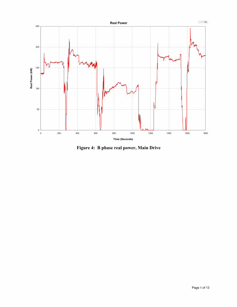
Page 5 of 13

Real Power

0

50

100

150

200

250

0 200 400 600 800 1000 1200 1400 1600 1800

Time (Seconds)

Rea

l Pow

er (k

W)

Pb

Figure 4: B phase real power, Main Drive

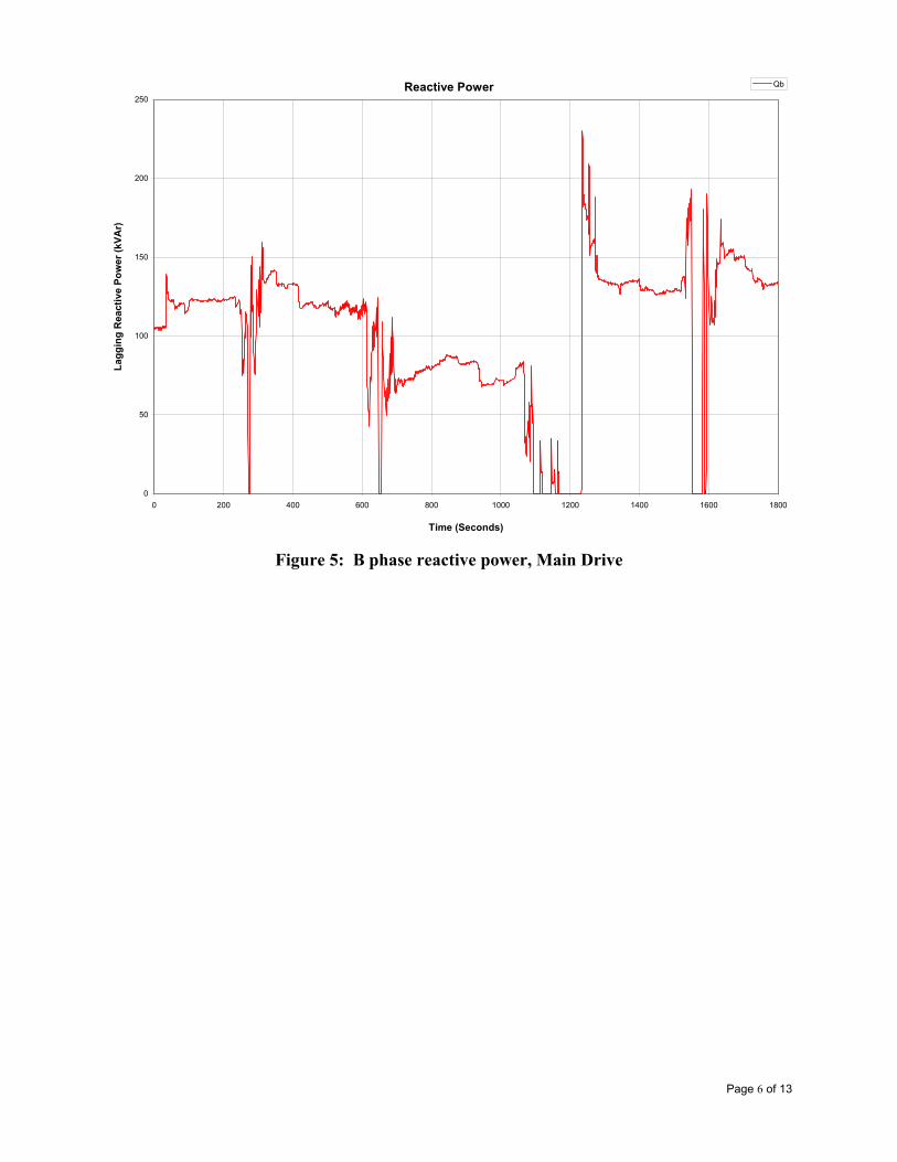
Page 6 of 13

Reactive Power

0

50

100

150

200

250

0 200 400 600 800 1000 1200 1400 1600 1800

Time (Seconds)

Lagg

ing

Rea

ctiv

e Po

wer

(kVA

r)

Qb

Figure 5: B phase reactive power, Main Drive

Page 7 of 13

Total Real Power

1000

1200

1400

1600

1800

2000

2200

0 200 400 600 800 1000 1200

Time (Seconds)

Rea

l Pow

er (k

W)

Ptotal

Figure 6: Total real power, Billing Meter

Page 8 of 13

Total Reactive Power

900

1000

1100

1200

1300

1400

1500

1600

1700

1800

0 200 400 600 800 1000 1200

Time (Seconds)

Lagg

ing

Rea

ctiv

e Po

wer

(kVA

r)

Qtotal

Figure 7: Total reactive power, Billing Meter

3.0 Analysis

The plant real power during the measurement period was between 1000 kW and 1900 kW. The reactive power was between 900 kVAr and 1650 kVAr. Power factor varied from 0.5 to 0.9 lagging. To achieve a 0.95 leading power factor, 1650 capacitive VArs would be needed to cancel out the mill’s lagging VArs plus an additional 625 VArs to make the mill go leading. There was between 19% and 34% unbalance present in the load current which can be seen in Figure 8. A single phase load appears to be connected between the A and B phases resulting in similar A and B phase currents and a 33% lower C phase current. There was less then 0.2% unbalance observed in the 20 kV voltage measured at the billing meter.

Page 9 of 13

Current

20

30

40

50

60

70

80

0 200 400 600 800 1000 1200

Time (Seconds)

Cur

rent

(A)

IaIbIc

Figure 8: Phase current, Billing Meter

A 480 kVAr (30%) step change in reactive power resulted in a 0.5% change in voltage at the billing meter. For this event, the change in reactive current was 13.9 A. The reactive current flowing through the system impedance to this point caused a drop of around 60 V. Assuming the system is dominated by X, and therefore has a relatively low R, the system impedance works out to be about 4.3 ohms. The short circuit capacity at this point would be 2685 A (93 MVA). This indicates the system is stiff enough to not result in significant voltage drop due to the Signode load. The load current contained between 10% and 25% THD, depending on the phase. The phase A and B current contained about 20% 3rd harmonic and 10% 5th. Phase C current had little 3rd and 10% 5th harmonic. Figure 9 shows a few cycles of the instantaneous current waveform. There was less then 3.0% THD measured in the voltage at the billing meter. Most of the voltage THD is due to 5th harmonic content. The phase A voltage had slightly higher 5th harmonic content (2.2%) while B and C phase were both around 1.9%. Figure 10 shows a few cycles of the instantaneous line to neutral phase voltages recorded at the billing meter.

Page 10 of 13

Current

100.950 100.960 100.970 100.980 100.990

-125

-100

-75

-50

-25

0

25

50

75

100

125 C

urre

nt (A

)

Ia Ib Ic

Figure 9: Instantaneous current, Billing Meter

Voltage

9.000 9.010 9.020 9.030 9.040 9.050

-20.0k

-15.0k

-10.0k

-5.0k

0.0

5.0k

10.0k

15.0k

20.0k

Volta

ge (V

)

Va Vb Vc

Figure 10: Instantaneous voltage, Billing Meter

Page 11 of 13

Figures 11, 12 and 13 show the spectra of phases A, B and C current respectively. Each column in the graph represents a harmonic. The far left column is the fundamental, the second column is second harmonic, the third column is the third harmonic and so on. The Y axis scale is in amps RMS. Phases A and B have similar spectra consisting mainly of 3rd and 5th harmonics. The 3rd harmonic content in these two phases is likely because of the single phase load. The C phase current has a much smaller 3rd harmonic content. Table 1 lists the harmonic content of Figures 11, 12 and 13 numerically.

IaHarm65.0

0.0

[1] 58.1084 Figure 11: A phase current spectrum, Billing Meter

Page 12 of 13

IbHarm65.0

0.0

[1] 56.4759 Figure 12: B phase current spectrum, Billing Meter

IcHarm

65.0

0.0

[1] 37.0686 Figure 13: C phase current spectrum, Billing Meter

Page 13 of 13

Phase A (Figure 11) Harmonic 1 2 3 4 5 6 7 8 9 10 11 12 13 14 15 Current (A) 58.11 0.09 9.62 0.06 5.59 0.12 2.29 0.07 1.03 0.04 0.71 0.05 0.45 0.05 0.35

Phase B (Figure 12) Harmonic 1 2 3 4 5 6 7 8 9 10 11 12 13 14 15 Current (A) 56.48 0.26 9.78 0.08 3.66 0.08 2.04 0.10 1.03 0.06 0.20 0.03 0.46 0.04 0.29

Phase C (Figure 13) Harmonic 1 2 3 4 5 6 7 8 9 10 11 12 13 14 15 Current (A) 37.07 0.02 0.48 0.07 4.00 0.06 0.44 0.02 0.08 0.05 0.89 0.06 0.05 0.02 0.10

Table 1: Harmonic Content, Billing Meter 3.0 S&C Solution

One method of improving the power factor at Signode would be to install an S&C PureWave® AVC System. The AVC uses discrete steps of thyristor switched capacitors to supply reactive compensation on a cycle by cycle basis. The AVC would measure the reactive portion of load current and then match the lagging current by switching in the proper number of capacitor stages. This can be done on a per phase basis which would work best for an unbalanced load like the Signode mill. Typically the AVC attempts to exactly match the reactive current and therefore would bring the power factor up to around 1.0. However, the controls can be configured to “over compensate” the lagging reactive current that is seen flowing to the load which would result in a leading power factor. Compensating the lagging reactive current also helps to limit the effect the load has on the system voltage by locally providing the necessary VArs. This results in less voltage drop across the system impedance. To achieve a 0.95 leading power factor at the Signode mill, a 2500 kVAr AVC would be required. The AVC would be preferable to slower, conventional switched capbanks because it can compensate faster transients and maintain a more consistent power factor. The AVC can also provide a “finer” compensation because it can switch capacitors on in up to 15 discrete steps, allowing for a closer match to the required compensation.

Appendix 9 — A Summary of Compensation Methods for Reactive Power for a Selection of Independent System Operators

1. ISO-NE

The ISO-NE’s Schedule 2 (ISO-NE Tariff, p.311) sets forth how generators providing voltage support will be compensated; and how the costs of providing this service will be allocated. As in most other ISOs, generation facilities are directed from time to time to operate to produce or absorb reactive power. To the extent that they are directed to produce (or absorb) reactive power, generation facilities are compensated for certain costs related to VAR control. The ISO-NE reimburses generators for four different kinds of costs related to voltage support, and the cost of voltage support is then spread to transmission customers (Load Serving Entities) based on load ratio share.

Payments for VS Procurement

Schedule 2 compensates for four (4) types of costs related to VAR control: Capacity Cost (CC) Lost Opportunity Cost (LOC) Cost of Energy Consumed (SCL) Cost of Energy Produced (PC)

Capacity Cost

The Capacity Costs is a payment that compensates generators for the equipment needed to deliver VARs to the system. This is a fixed payment system based on the Capacity Cost VAR Rate which is an annual formula rate calculation, established at the beginning of the year and in effect for the calendar year. The CC VAR Rate is a construct of the Base VAR Rate (currently set at $1.05/kVARyr) and a “Factor” which is either , or sometimes less than one if there is “excess” generator VAR capability. CC VAR Rate = Base VAR Rate * Factor Where: Base VAR Rate = $1.05 / kVAR-yr

Factor equals 1 or less than 1, if there is "excess" generator VAR capability.

Lost Opportunity Cost (LOC)

LOC is a payment that compensates generators if ISO, a Local Control Center or a "dispatch center" reduces the output of an on-line hydro, pumped storage or thermal generating unit for the purpose of VAR control. This is a variable compensation mechanism, and the compensation is equal to (the energy that the generator would have sold in an hour had it not been backed down for VAR control) * (LMP in that hour). This is conceptually similar to the LOC payment that the CAISO makes to generating units that it backs down to boost VARS during peak load conditions.

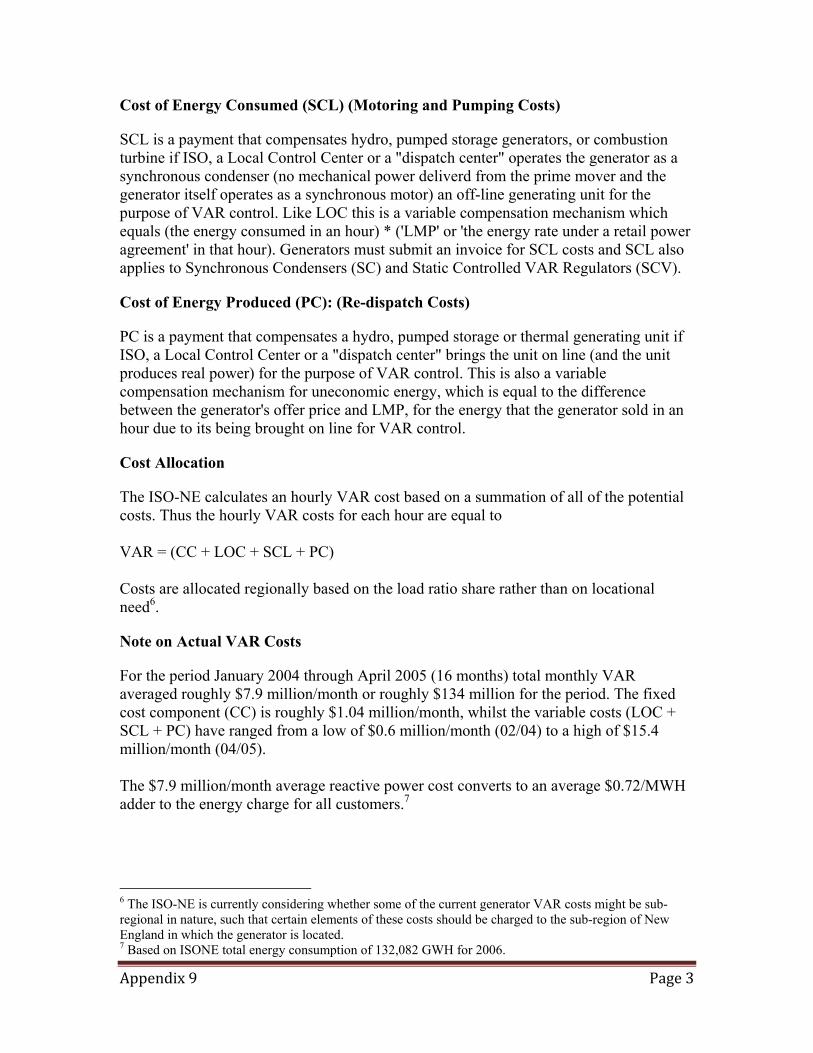
Cost of Energy Consumed (SCL) (Motoring and Pumping Costs)

SCL is a payment that compensates hydro, pumped storage generators, or combustion turbine if ISO, a Local Control Center or a "dispatch center" operates the generator as a synchronous condenser (no mechanical power deliverd from the prime mover and the generator itself operates as a synchronous motor) an off-line generating unit for the purpose of VAR control. Like LOC this is a variable compensation mechanism which equals (the energy consumed in an hour) * ('LMP' or 'the energy rate under a retail power agreement' in that hour). Generators must submit an invoice for SCL costs and SCL also applies to Synchronous Condensers (SC) and Static Controlled VAR Regulators (SCV).

Cost of Energy Produced (PC): (Re-dispatch Costs)

PC is a payment that compensates a hydro, pumped storage or thermal generating unit if ISO, a Local Control Center or a "dispatch center" brings the unit on line (and the unit produces real power) for the purpose of VAR control. This is also a variable compensation mechanism for uneconomic energy, which is equal to the difference between the generator's offer price and LMP, for the energy that the generator sold in an hour due to its being brought on line for VAR control.

Cost Allocation

The ISO-NE calculates an hourly VAR cost based on a summation of all of the potential costs. Thus the hourly VAR costs for each hour are equal to VAR = (CC + LOC + SCL + PC) Costs are allocated regionally based on the load ratio share rather than on locational need6.

Note on Actual VAR Costs

For the period January 2004 through April 2005 (16 months) total monthly VAR averaged roughly $7.9 million/month or roughly $134 million for the period. The fixed cost component (CC) is roughly $1.04 million/month, whilst the variable costs (LOC + SCL + PC) have ranged from a low of $0.6 million/month (02/04) to a high of $15.4 million/month (04/05). The $7.9 million/month average reactive power cost converts to an average $0.72/MWH adder to the energy charge for all customers.7

6 The ISO-NE is currently considering whether some of the current generator VAR costs might be sub-regional in nature, such that certain elements of these costs should be charged to the sub-region of New England in which the generator is located. 7 Based on ISONE total energy consumption of 132,082 GWH for 2006.

References

ISO-NE OATT Available on page 249-258 (Sheet 735) http://www.iso-ne.com/regulatory/tariff/sect_2/oatt/section2_of_rto_tariff.pdf ISO-NE VAR Settlement Presentation provided to the CAISO.

2. NYISO

The NYISO has a two part payment system for Voltage Support. It provides a fixed payment to all generators and synchronous condensers and also reimburses them for the LOC of dispatches that entail the reduction (or consumption) of real power.

Payments for VS Procurement

The NYISO tariff states that the annual payment to each Generator and synchronous condenser qualified and eligible to provide Voltage Support Service (VSS) shall equal the product of $3919/MVAr and the tested MVAr capacity of the Generator or synchronous condenser. The NYISO makes a distinction in its payments depending on whether or not the generator in question provides installed capacity.

Fixed Payments

Generators Providing Installed Capacity If a non-utility Generator provides installed capacity, the NYISO will pay it monthly the product of: (1) one -twelfth of the annual $/MVAr rate for NYISO payments to Suppliers of VSS and (2) the lesser of the tested Reactive Power production capability (MVAr) of the Non-Utility Generator or the contract MVAr capability.

Generators Not Providing Installed Capacity If a non-utility Generator does not provide Installed Capacity, the NYISO will pay it the product of (1) and (2), as calculated above, multiplied by the number of hours in the month the Non-Utility Generator provided VSS divided by the number of hours in the month.

Variable Payments

A Supplier providing VSS from a Generator that is In-Service is entitled to receive Lost Opportunity Costs (LOCs) in the event the NYISO dispatches or directs the Generator to reduce its real power (MW) output in order to allow the unit to produce or absorb more reactive power (MVAr). The method used by the NYISO for calculating the LOC is similar to that used elsewhere, in that the LOC is defined as the distance between the bid_price and the LMP. This is then calculated for the reduction in MWs ordered by the NYISO. The NYISO calculates and makes payments on a monthly basis.

Alan – they also pay for energy consumed by synchronous condensers or generators running in the condensing mode don’t they? - BJK

Cost Allocation

NYISO basically allocates the reactive power costs on a load ratio share. Transmission Customers and Load Serving Entity (LSEs) taking service under the NYISO OATT pay the NYISO for VSS associated with energy withdrawals from the transmission system. The NYISO computes the VSS Rate as follows: The sum of the projected NYISO payments to Suppliers providing Voltage Support including:

Total annual costs eligible for payment Any applicable Lost Opportunity Costs to provide VSS Total of prior year payments to Suppliers of VSS less the total of payments

received by the NYISO from Transmission Customers and LSEs in the prior year for VSS including all payments for penalties [this line item allows the carry forward of costs to ensure complete revenue recovery]

This sum is divided by annual forecasted transmission usage for the year as projected by the NYISO, including Load within the NYCA, Exports, and Wheels Through. Transmission Customers engaging in Wheels-Through or Exports pay to the NYISO a charge for this service equal to the rate as determined above multiplied by their Energy wheeled in the hour. Load Serving Entities serving loads in the NYCA pay to the NYISO a charge for this service equal to the hourly rate as determined above multiplied by the Energy withdrawn from the transmission system in order to serve that LSEs Load in the hour. The NYISO calculates the payment hourly and bills each Transmission Customer or LSE monthly.

Alan – did you find a total annual $ number? If so we can use NYISO’s annual energy of 162,500 GWH to get an average $/MWH allocation.

References

NYISO “Ancillary Services Manual” Available at http://www.nyiso.com/public/documents/manuals/operations.jsp?maxDisplay=20 NYSIO Tariff (Rate Schedule 2 – starting page 9) Available at http://www.nyiso.com/public/webdocs/documents/tariffs/market_services/rate_schedules.pdf

3. PJM

The PJM provision of voltage support seems to differ from that elsewhere in that Reactive Supply and Voltage Control from Generation Sources is provided directly by the Transmission Provider’s in their service territories. PJM itself does not seem to provide or procure voltage support. Rather each generation owner establishes a Reactive revenue requirement that they get approved by FERC. This is then specified in the PJM tariff for each service territory. PJM aggregates these generator revenue requirements by zone with each generator's revenue requirement being assigned to the specific zone in which it is located. PJM then allocates these revenues to the load in the applicable zone with a pro rata portion being charged to point-to-point transmission customers taking through and out service.

Alan – Were you able to tell if PJM or anyone else determines a need for the reactive power capability before granting the generator the revenue? I know that in MISO at least for a time there was not check of need. So a generator that did not even ever run could collect as much revenue as it wanted based on building unneeded reactive capability. I hope PJM does not allow that. FERC, of course, has no ability to technically determine need. – BJK

Payments for Voltage Support Procurement

Monthly credits are provided to generation and transmission owners with FERC-approved reactive revenue requirements (or generation owners with revenue requirements assigned to them by former generation owner). The owner’s monthly credit is equal to 1/12th of their annual reactive revenue requirement as shown in Schedule 2 of the Tariff. This is a fixed payment.

Variable Payments

PJM does not appear to have a facility to reimburse generators for variable payments.

Cost Allocation

Monthly pool-wide reactive revenue requirements are allocated as charges to point-to-point customers (and to network customers in transmission zones with no reactive revenue requirements) based on their monthly peak usage of the PJM transmission system. Monthly peak usage equals the total hourly amounts of transmission capacity reserved, and not curtailed by PJM, divided by 24. The remaining reactive revenue requirements for each transmission zone not recovered from point-to-point customers are allocated to the network customers and point-to-point customers serving load in that zone based on their monthly peak loads. Monthly peak loads equal the sum of all daily network service peak load contributions.

Figure 1: Example of the Publicly Available Revenue Requirement for Atlantic Electric as in PJM Tariff

References

PJM (2006) Schedule 2 of the PJM tariff, page 396, Revised Sheet No. 228, Available at: http://www.pjm.com/documents/downloads/agreements/tariff.pdf

4. ERCOT

ERCOT appears to have a system much like the current CAISO system in that generators are not compensated for providing Voltage Support except when their real power output changes.

Payments for VS Procurement

(1) Uncompensated Reactive Support - Generation Entities are required to maintain a voltage regulation schedule without compensation limited to the quantity of reactive power the Generation Resource can produce at rated capability, (MW), and a power factor of .95 leading or lagging (Unit Reactive Limit - URL) measured at the unit main transformer high voltage terminals.

(2) Compensated Reactive Support - If the ERCOT instructs the Generation Resource to exceed the URL, then the ERCOT will pay for the additional reactive power provided beyond the URL at a price that recognizes the avoided cost of reactive support Resources on the transmission network.

(3) Compensation for Power Reduction – Compensation for real power reduction to allow voltage support will be compensated as OOME Down, as specified in Section 6.8.2.2(4), Energy Payments, of the Protocols8.

Cost Allocation

As most of the ERCOT voltage support is uncompensated there are few charges, but to the extent that there are charges they are charged on a Load Ratio share basis (ERCOT, 2006 Section 6.9.3)

References

ERCOT (2006) Protocols Section 6. Available at: http://www.ercot.com/mktrules/protocols/current.html

8 This is defined as : “Generation Resources that are connected to the ERCOT Transmission Grid when their QSE is instructed to provide OOMC Service will be paid the Resource Category Generic Minimum Energy Cost less the MCPE for operating at the Low Sustainable Limit of the Resource during the instructed interval(s).”

5. Other Jurisdictions9

Columbia

Chang et.al.(2003) of the Brattle Group, a consultancy, detail a case study of the Columbian power system, a deregulated market with a system administrator responsible for the overall security of the grid. In that paper they detail a framework in which there are four classes of reactive support, namely;

Mandatory Reactive Support: reactive support provided as a condition of participation, is specified as an available MVAr, and is not recompensed. Substitute Reactive Support: via a bulletin board the SA (System Administrator) facilitates the trade in the mandatory reactive support component from generating units in electrically equivalent zones. Trades are done bilaterally. Supplemental Reactive Support: a visible spot market supplying only a small proportion of reactive power needs via a yearly auction process. Procurement is zonal to ensure product substitutability and prices are capped to prevent local market power abuses. Exceptional Reactive Support: the SA can call on any unit in exceptional circumstances and will reimburse them via a LOC payment.

England and Wales

The National Grid is the authority responsible for running the electricity grid in England and Wales. It appears they have had a competitive reactive power market for some time. National Grid (2005) documents the sixteenth tender round of a process that seems to have two tender rounds per year for contracts that are either 12,18 or 24 months long. It appears that generators tender to provide the reactive power service and are evaluated according to public criteria developed by the National Grid. The tenders are ranked and offered contracts based on their tenders and their benefits to the grid. Not all entities take up the offered tenders. The process appears to be backstopped by a Default Payment Mechanism to ensure some level of base case reliability. The FERC staff report points out that the system operator sends the generator a dispatch signal consisting of the amounts of real power and reactive power within a range of the required generator capability. A generator can accept a default payment for reactive power of approximately $2.40/Mvarh leading or lagging, or as an alternative, the generator may offer contracts with a minimum term of one year. The offer consists of three parts: a synchronized capability price in £/ MVAR, an availability capability price in £/MVAR and a utilization price in £/ Mvarh. The grid company assesses the offer, historical performance and effectiveness of each generator against its locational forecast needs in about 20 electrical zones to decide which offers to accept. This provides generators incentives to offer

9 FERC had a technical conference on Reactive Power and there is much documentation there (Docket No. AD05-1-000):

capability beyond the requirements, lowering investment requirements for the transmission system.

References

Chang, J.W. Graves, F.C., Murphy, D.M. (2003) “Transmission Management in the Deregulated Electric Industry: A Case Study on Reactive Power” Electricity Journal, October 2003, 61-73 National Grid (2005) “Reactive Power Market” November 2005. Available at: http://www.nationalgrid.com/uk/Electricity/Balancing/archivedmaterial/tenders/