o in PLS Path Models for Composite Indicators · NTTS 2009, February 18th-20th 2009! o Role and...

NTTS 2009, February 18th-20th 2009!

Laura Trinchera & Giorgio Russolillo!Role and treatment of categorical variables

in PLS Path Models for Composite Indicators

Laura Trinchera1,2 & Giorgio Russolillo2 !1Dipartimento di Studi sullo Sviluppo Economico, Università degli Studi di Macerata

2Dipartimento di Matematica e Statistica, Università degli Studi di Napoli “Federico II”


Talk outline

  Part I: Using Structural Equation Models and PLS Path Modeling to build systems of Composite Indicators

  Part II: Categorical Variables as moderating variables

  Manifest Moderating variables   Latent Moderating variables

  Part III: Categorical Indicators as manifest variables   Modified PLS Path Modeling algorithm

  Part IV: An example with RUSSET data

  Conclusion and Perspectives

Laura Trinchera & Giorgio Russolillo!



Part I

Composite Indicators (CIs) are mathematical combinations of single quantitative indicators representing different dimensions of the concept

to be measured (Saisana et al., 2002)

The main feature of a CI is that it summarizes complex and multidimensional issues

Each CI is not only a composite indicators but also a complex indicator due to the causal relations with the other CIs

Introduction

Structural Equation Models (SEMs) are complex models allowing the study of real world complexity by taking into account a number of causal relationships among latent concepts (i.e. the CIs), each measured by several observed indicators usually defined as Manifest Variables.


Structural Equation Models

ξ3

x11

x21

x31

x12

x13

x22

x23

x33

x43

x53

•  P manifest variables or indicators (MVs ) observed on N units

•  Q latent variables or Composite Indicators (LVs) •  Q blocks composed by each LV and the corresponding MVs

xpq generic MV ξq generic LV

in each q-th block pq manifest variables xpq , with

Inner or Structural model Outer or Measurement model

Path Coefficients

β1

β2 λ12

λ22

Loadings

ξ1

ξ2

€

pqq=1

Q

∑ = P


Part I



Part I

PLS Path Modeling (PLS-PM) (Wold, 1975) and (Tenenhaus et al., 2005)

It is an iterative algorithm that allows us to estimate the LV scores through a system of interdependent linear equations modeling the relations among the MVs and their corresponding LV and among the LVs of the model

The LV scores (i.e. the CIs) are obtained so as to be the most representative of each block of indicators and the most correlated with one another

(according to path diagram)

•  it is always identified •  it is a distribution-free technique

•  the LV scores are “directly” obtained

•  PLS-PM convergence is assured in practice, but it is not proved •  PLS-PM does not maximizes a unique function

PLS-PM pro and cons :



Part I

A schematic representation of the PLS-PM algorithm

Mode A: wq = (1/n)Xʼqzq Mode B: wq = (XʼqXq)-1Xʼqzq

Initialization step

vq ∝ ± Xqwq

v1

vqʼ

zq

e1q

e2q

eqʼq

v2

PLS Path Modeling (PLS-PM)

wq

Choice of weights eqʼq: - Centroid: correlation signs - Factorial: correlations -  Path weighting scheme: multiple regression coefficients or correlations


Categorical Variables in PLS-PM Laura Trinchera &

Giorgio Russolillo!Part I

Categorical Variables can play two different roles in a PLS Path Model:

Active categorical variables --> are variables directly participating in computing LV scores

Moderating categorical variables --> are variables influencing the relations, in terms of strength and/

or direction, between an exogenous and an endogenous variable

The moderating effect can be seen as the effect obtained by considering several groups of units

Categorical variables are indicators (MVs) in a PLS Path Model


Moderating Categorical Variables Laura Trinchera &

Giorgio Russolillo!Part II

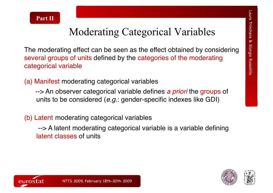
The moderating effect can be seen as the effect obtained by considering several groups of units defined by the categories of the moderating categorical variable

(a) Manifest moderating categorical variables --> An observer categorical variable defines a priori the groups of

units to be considered (e.g.: gender-specific indexes like GDI)

(b) Latent moderating categorical variables --> A latent moderating categorical variable is a variable defining latent classes of units



Part II (a)

Manifest Moderating Categorical Variables

ξ1 ξ3

Moderating variable

x11

x21

x13

x23

x33

x43

x53

xm

xm is a categorical variables defining classes, for instance the gender variable

Several techniques has been proposed to consider xm in a PLS Path Model:

--> by including interaction term as the product of the indicators linked to the exogenous LV and the categories of the moderating variable (Chin et. al, 2003)

--> by including interaction term trough a two steps procedure (first define the LV scores and then used these variables to obtain interaction terms) (Henseler et. al, 2009) --> by considering the interaction term in the sense of Chin et al. (2003) but removing the redundant information (Tenenhaus et. al, 2009)


Latent Moderating Categorical Variables Laura Trinchera &

Giorgio Russolillo!Part II (b)

We search for latent classes showing different models, i.e. local models

Hahn et al. (2002)

Squillacciotti (2005) Trinchera et al. (2006)

Sánchez and Aluja (2006)

A Priori Segmentation

Simultaneous Segmentation and Estimation

PATHMOX

PLS Typological Path Modeling

Finite Mixture PLS Clustering in

PLS-PM

Trinchera (2007), Esposito Vinzi et al. (2008)

REBUS-PLS

Several techniques have been proposed to obtain response-based unit clustering in PLS-PM :

These techniques allow us to obtain groups of units homogenous with respect

to the weights used to compute the CIs



Part III

Categorical Variables as MVs

ξ3

x11

x21

x31

x*12

x13

x22

x23

x33

x43

x53

ξ1

ξ2

x*12 is a categorical indicator, e.g. type of government

Usually x*12 is replaced by the corresponding dummy-matrix , but:

--> The number of indicators increases (we have as many indicators as the categories of categorical indicator are) --> The impact of each categories is measured, but no information about the role of the categorical indicator as a whole €

˜ X 12

Optimal scaling of categorical indicators



Part III

Categorical Variables as MVs

We extend PLS-CAP regression algorithm by Russolillo (2008) to PLS-PM

Each categorical indicator x*pq is quantified in such a way that its weight in building the corresponding LV score is a function of the LV variance explained by x*pq categories, in particular:

€

x pq ∝ ˜ X pq ˜ ′ X pq ˜ X pq( )−1 ˜ ′ X pqzq€

cor x pq ,zq( ) =ηx pq* ,zq

where xpq is the quantified indicator obtained as the normalized orthogonal projection of the inner estimate of the LV (zq) on the space spanned by the columns of :

€

˜ X pq



Part III

Categorical Variables as MVs Modified PLS-PM algorithm to handle qualitative indicators

Mode A: wq = (1/n)Xq’zq Mode B: wq = (Xq’Xq)-1Xq’zq

vq ∝ ± Xqwq

v1

vq’

zq

e1q

e2q

eqʼq

v2

€

x pq ∝ ˜ X pq ˜ ′ X pq ˜ X pq( )−1 ˜ ′ X pqzq

Initialization step

zq



Part IV Real case example:

data from RUSSET (1964)

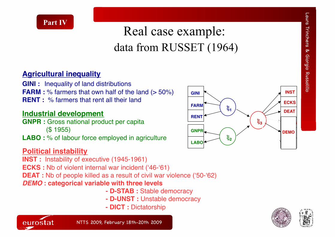
Agricultural inequality GINI : Inequality of land distributions FARM : % farmers that own half of the land (> 50%) RENT : % farmers that rent all their land

Industrial development GNPR : Gross national product per capita ($ 1955) LABO : % of labour force employed in agriculture

Political instability INST : Instability of executive (1945-1961) ECKS : Nb of violent internal war incident (ʻ46-ʻ61) DEAT : Nb of people killed as a result of civil war violence (ʻ50-ʻ62) DEMO : categorical variable with three levels - D-STAB : Stable democracy - D-UNST : Unstable democracy

- DICT : Dictatorship

GINI

FARM

RENT

GNPR

LABO

ξ1

ξ2

ECKS

DEAT

D-STB

D-INS

INST

DICT

ξ3

DEMO



Part IV

Agricultural Inequality

Industrial Development Political Instability

GINI

FARM

RENT

GNPR

LABO

ξ1

ξ2

ECKS

DEAT

D-STB

D-INS

INST

DICT

ξ3

Real case example: results for the model with dummy variables

GoF = 0.618

.459

.528

.082

.522

-.550

.105

.274

.295

-.346 .024

.305

.21

-.70 R2=.626

Communality =0.731

Communality =0.907

Communality =0.452



Part IV



GINI

FARM

RENT

GNPR

LABO

ξ1

ξ2

ECKS

DEAT

DEMO

INST

ξ3

Real case example: results for the model with the quantified variable

GoF = 0.645

R2=.594

.464

.514

.118

.525

-.547

.129

.336

.365

.449

.228

-.669

Communality =0.571

Communality =0.736

Communality =0.908



Part IV



GINI

FARM

RENT

GNPR

LABO

ξ1

ξ2

ECKS

DEAT

INST

ξ3

Real case example: results for the model without DEMO

GoF = 0.562 .442

.461

.244

.538

-.534

.194

.504

.561

.273

-.531 R2=.436

Communality =0.749

Communality =0.908

Communality =0.578


--> However, each CI can be seen also as a complex indicator, obtained according to the others Cis in the model, in particular each endogenous LV can be predicted also trough the exogenous LVs and the path coefficients:


Part IV Real case example:

Conclusions

Political instability (ξ3) = 0.13×INST+0.34×ECKS+0.37×DEAT+0.45×DEMO

To conclude, categorical indicators can be used as MVs in a reflective PLS-PM by means of our modified PLS-PM algorithm

Political instability ( ) = 0.23×Agricultural ineq.(ξ1) -0.67× Industrial dev.(ξ2)

€

ˆ ξ 3

According to the results obtained trough the modified PLS-PM algorithm --> The LV scores, i.e. the Cis, are obtained as linear combination of the corresponding indicators, e.g. for the CI “Political Instability”:


Conclusions and perspectives

  Constrained PLS-PM should be developed in order to include a priori information on the weights defining composite indicators

  The identification of the compromise model need to be further investigate


  The effect of the number of categories of a categorical indicator on the quantification need to be study


1. Baron R.M. and Kenny D.A., The Moderator-Mediator Variable Distinction in Social Psychological Research: Conceptual, Strategic, and Statistical Considerations, Journal of Personality and Social Psychology, 51 (6), 1173-1182 (1986). 2. Bollen K. A., Structural equations with latent variables, Wiley, New York (1989). 3. Chin W.W., A permutation procedure for multi-group comparison of PLS models, in PLS and related methods - Proceedings of the International Symposium PLS’03, M. Vilares et al. (eds), DECISIA, 33-43 (2003). 4. Escofier B. and Pagés J., Multiple factor analysis (AFMULT package), Computational Statistics and Data Analysis, 18,121-140 (1994). 5. Esposito Vinzi V., Trinchera L., Squillacciotti S. and Tenenhaus M., REBUS-PLS: A Response–Based Procedure for detecting Unit Segments in PLS Path modeling, Applied Stochastic Models in Business and Industry, (2008). 6. Hahn C., Johnson M., Herrmann A. and Huber F., Capturing Customer Heterogeneity using a Finite Mixture PLS Approach, Schmalenbach Business Review, 54, 243-269 (2002). 7. Hensler J. and Fassott G., Testing moderating effects in PLS path models: An illustration of available procedure, in Handbook of Partial Least Squares - Concepts, Methods and Applications, V. Esposito Vinzi et al. (eds), Springer, Berlin, Heidelberg, New York (2009). 8. Russolillo G., A proposal for handling categorical predictors in PLS regression framework. in First joint meeting of the Socit Francophone de Classification and the Classification and Data Analysis Group of the Italian Statistical Society. Book of short papers, Edizioni Scientifiche Italiane, 401 (2008). 9. Saisana M. and Tarantola S. State-of-the-art Report on Current Methodologies and Practices for Composite Indicator Development, EUR 20408 EN, European Commission-JRC: Italy (2002). 10. Tenenhaus M., Esposito Vinzi V., Chatelin Y.-M. and Lauro C., PLS Path Modeling, Computational Statistics and Data Analysis, 48, 159-205 (2005). 11. Trinchera L., Unobserved Heterogeneity in Structural Equation Models: a new approach in latent class detection in PLS Path Modeling, PhD thesis, DMS, University of Naples (2007).

Main references Laura Trinchera &

Giorgio Russolillo!

o in PLS Path Models for Composite Indicators · NTTS 2009, February 18th-20th 2009! o Role and...

Documents

Transcript of o in PLS Path Models for Composite Indicators · NTTS 2009, February 18th-20th 2009! o Role and...