NUREG/CR-5583KEI No. 1656

I Prediction of Check ValvePerformance and Degradationin Nuclear Power Plant Systems --

Wear and Impact Tests

Final ReportSeptember 1988 - April 1990

Prepared by M. S. Kalsi, C. L Horst, 3. K. Wang, V. Sharma

Kalsi Engineering, Inc.

Prep re-d for,t U.S. Nuclear Regulatory Commission

I

I ,

AVAILABILITY NOTICE

Availability of Reference Materials Cited In NRC Puications

Most documents cited In NRC pubicatlons wUl be available from one of the following sources:

1. The NRC Publo Document Room. 2120 L Street, NW, Lower Level. Washington. DC 20555

2. The Superintendent of Documents, U.S. Government Printing office. P.O. Box 37082, Washington,DC 20013-7082

3. The National Technical Information Service, Springfield, VA 22161

Although the Isting that follows represents the majority of documents cited In NRC publications, It Is notIntended to be exhaustive.

Referenced documents available for Inspection and copying for a fee from the NRC Pubic Document RoomInclude NRC correspondence and Internal NRC memoranda; NRC Office of Inspection and Enforcementbulletins, crculars, Information notices, Inspection and Investigation notices; Ucensee Event Reports; ven-dor reports and correspondence; Commission papers; and applicant and licensee documents and corre-spondence.

The following documents In the NUREG series are available for purchase from the GPO Sales Program:formal NRC staff and contractor reports, NRC-sponsored conference proceedings, and NRC booklets andbrochures. Also available are Regulatory Guides, NRC regulatons In the Code of Federal Regulations, andNuclear Regulatory Commission Issuances.

Documents available from the National Technical Information Service Include NUREG series reports andtechnical reports prepared by other federal agencies and reports prepared by the Atomlo Energy Commls-ston, forerunner agency to the Nuclear Regulatory Commission.

Documents available from pubic and special technical libraries Include al open literature Items, such asbooks, journal and periodical articles, and transactions. Federal Register notices, federal and state legisla-tion, and congressional reports can usually be obtained from these libraries.

Documents such as theses, dissertations, foreign reports and translations, and non-NRC conference pro-ceedings are available for purchase from the organization sponsoring the publication cited.

Single copies of NRC draft reports are available free, to the extent of supply, upon written request to theOffice of Information Resources Management, Distrlbution Section, U.S. Nuclear Regulatory Commisslon.Washington, DC 20555.

CopIes of Industry codes and standards used hI a substantive manner In the NRC regulatory process aremaintained at the NRC Library, 7920 Norfolk Avenue, Bethesda, Maryland, and are available there for refer-ence use by the public. Codes and standards are usually copyrighted and may be purchased from theoriginating organization or. If they are American National Standards, from the American National StandardsInstitute, 1430 Broadway, New York, NY 10018.

DISCLAIMER NOTICE

This report was prepared as an account of work sponsored by an agency of the United States Government.Neitherthe United States Government nor any agencythereol, or any oftheir employees, makes any warranty,expresed or Implied, or assumes any legal liability of responsibility for any third paty's use, or the results ofsuch use, of any Information, apparatus, product or process disclosed In this report, or represents that Its useby such third party would not Infringe privately owned rights.

NUREG/CR-5583KEI No. 1656RG, RV

Prediction of Check ValvePerformance and Degradationin Nuclear Power Plant Systems --

Wear and Impact TestsFinal ReportSeptember 1988 - April 1990

Manuscript Completed: May 1990Date Published: August 1990

Prepared byM. S. Kalsi, C. L. Horst, J. K. Wang, V. Sharma

W. S. Farmer, NRC Project Manager

Kalsi Engineering, Inc.745 Park Two DriveSugar Land, TX 77478

Prepared forDivision of EngineeringOffice of Nuclear Regulatory ResearchU.S. Nuclear Regulatory CommissionWashington, DC 20555NRC FIN D2510

ABSTRACT

Check valve failures in nuclear power plants have led to safety concerns as well as'extensive damage and loss of plant availability in recent years. Swing check valveinternals may experience premature deterioration if the disc is not firmly held openagainst its stop. At the present time no guidelines exist for the prediction of degradationtrends and the determination of suitable inspection intervals.

This research Is aimed at developing a reliable quantitative wear and fatigue predictionmodel for swing check valves which can be used to improve the safety and reliability oftheir operation. Additionally, the predictive techniques can be used to augment checkvalve preventive maintenance programs by providing the plant engineer with quantitativeand conservative estimates of damage potential for check valve internals.

- iii -

TABLE OF CONFENTSPage

EXECUTIVE SUMMARY 1

INTRODUCTION 2Background 2Overall Research Objectives 2Phase I Research 2Phase II Research 3

WEAR PREDICTION 5Theoretical Wear Equation 5Wear Coefficient, K 5Sliding Distance 5Load 6

ACCELERATED WEAR TESTS 7General 7Valve and Hinge Pin Modifications for Wear Testing 9Selection of Materials to Accelerate Wear 9Preliminary Wear Tests, Accuracy of Measurements, and Eliminating Effects 12of Corrosion and ErosionMatrix of Accelerated Wear Tests 13

WEAR TEST RESULTS AND DISCUSSION 15

Accelerated Wear Test Results 15Normalized Wear Rates 19Comparison Between Theoretical Wear Prediction and Tests 2D

WEAR PREDICIION METHODOLOGY - SlUMARYAND CONCLUSIONS 2

IMPACT AND FATIGUE PREDICTIONS 23

Theoretical Prediction Techniques 23Disc Natural Frequency Approach 23Pipe Eddy Frequency Approach 24Mean and 3G Disc Speed Approach 24

IMPACT AND FATIGUE TESTING 25

General Methodology 25Test Valve 25Calibration of Strain Gaged Valve Disc 29Instrumentation 29

-V.

TEST RESULTS 3)Typical Impact Signature 30Discussion of Impact and Disc Motion Signals 2Discussion of Disc Motion Measurements and Modified Disc 33Use of 3a Disc Speed for Disc Impact Force Estimates 34Rate of Occurrence of Impacts 35

CORRELATION OF IMPACT TEST DATA TO THEORY 37Kinetic Energy Conversion Approach 37Disc Oscillation Amplitude and Frequency Approach 37

IMPACT FORCE AND FATIGUE PREDICTION MEHODOLOGY- 4

SUMMARY AND CONCLUSIONS

CORRELATION AGAINST PLANT DATA 41Plant Correlation Example 1: 4118-Inch Swing Check Valves with Excessive Hinge Pin Bushing WearPlant Correlation Example 2: 4418-Inch Swing Check Valves with Low Hinge Pin Bushing WearPlant Correlation Example 3: 444-Inch Tilting Disc Check Valve Modifications to Reduce Hinge Pin WearPlant Correlation Example 4: 4510" Swing Check Valve Disc Stud Fatigue Failure

SUMBIARY OF CHECK VALVE REVIEW OME ODOLOGY 47Overview of Check Valve Review and Analysis Procedure 47Vmin Calculation 47Calculation of Modified Vmin using Cup 60Wear and Fatigue Calculations 51Conclusions 51

REFERENCES

APPENDIX Az Impact and Fatigue Prediction MethodsAPPENDIX B.: Calculation of Vmin, Flow Velocity, and Wear Rate for

Plant Correlation Example 1APPENDIX C: Correlation of Fatigue Analysis with Available Plant Data

for Plant Correlation Example 4APPENDIXD-. Plots of Mean Disc Speed and 3-Sigma Disc Speeds for

the 3-Inch and 6-Inch Test Swing Check Valves

- vi -

LISr OF FIGURESFigure No.

1 Typical Swing Check Valve Geometry

2 Instrumented Test Valve

8 Valve Modifications for Accelerated Wear Tests

4 Modified Hinge Pin for Accelerated Wear Tests

6 Typical Aluminum Hinge Pin and Bushings Used in Wear Tests

6 Multihole Orifice Plates Used to Generate Turbulence

7 Typical Hinge Pin Wear Results for the 3-Inch Swing Check Valve(Upstream Disturbance: 36 x 3/16-Inch Hole Turbulence Plate at 2.5 D)

8 Accelerated Wear Test Results for the 3-Inch Valve

9 Accelerated Wear Test Results for the 6-Inch Valve

10 Comparison of Accelerated Wear Test Results to Theoretical Predictions

11 Instrumented Disc Cross Section

12 Strain Gage Bridge Schematics

13 Strain Gaged Check Valve Disc

14 Detail of Strain Gage Installation

15 Disc Showing Sealed Wire Exit

16 Wire Exit from Disc

17 Completion of Pressure Boundary Using Hermetic Connector

18 Impact Signature, Upstream Turbulence Source

19 Impact Signature, Upstream Elbow

23 Impact Signature, Upstream Turbulence (Modified Disc)

21 Raw and Filtered Impact Force Signatures

22 Disc Displacement Plot Corresponding to Impact Event of Figure 21

23 Impact Measurement Assembly

24 Impact Force Survey (Based on Filtered Signal, Ibs)

25 Impact Force Survey (Based on Filtered Signal, Ibs)

26 18-Inch Swing Check Valve Installation Used in Example 1

27 Hinge Pin Bushing Wear in 18-Inch Valves (Example 1)

28 Severe Hinge Pin Wear in 4-Inch Tilting Disc Check Valve

29 Minimum Velocity Formula Comparison Against Test Results

SD Significance of Disc Projection (Y/D) on Performance

Page

4

7

10

n

n

12

15

17

is21

26

26

26

27

27

28

26

31

31

31

32

33

34

96

36

42

43

44

48

49

- Vi-

L1ST OF TABLETable No. Page

LA Data for 3-Inch Valve 8

1B Data for 6-Inch Valve 8

2 Matrix of Hinge Pin Accelerated Wear Tests 14

3 Summary of Hinge Pin Accelerated Wear Tests 144 Summary of Test Parameters and Wear Rates Results of 16

Hinge Pin Accelerated Wear Tests

5 Disc Assembly Resonant Frequencies, hz 30

6 Impact Force Ranges (After Low-Pass Filtering) 357 Comparison of Theoretical and Measured Impact Forces 39

6-Inch Modified Disc Assembly; High Turbulence Sourceat 1.5 Diameters Upstream

- viii -

ACKNOWLEDGEMENTS

We are greatful for the funding provided by the Small Business Innovation Researchprogram of the U. S. Nuclear Regulatory Commission which made this research possible.Special thanks are due William S. Farmer of the NRC for his guidance andencouragement throughout the project.

The authors would also like to pay special recognition to Daniel Alvarez for thedevelopment of the load cell concept employed in these tests, and to Bobbie Lambert forpatiently working through many revisions and for her painstaking attention to detail inpreparing this manuscript.

- ix -

EXECUlMVE SUMMARY

Check valve failures at nuclear power plants in recent years have led to serious safetyconcerns, and caused extensive damage to other plant components which had a significantimpact on plant availability. In order to understand the failure mechanism and improvethe reliability of check valves, a systematic research effort was proposed by KalsiEngineering, Inc. to U.S. Nuclear Regulatory Commission (NRC) under their SmallBusiness Innovation Research (SBIR) program. The overall goal of the research was todevelop models for predicting the performance and degradation of swing check valves innuclear power plant systems so that appropriate preventive maintenance or designmodifications can be performed to improve the reliability of check valves.

Under Phase I of this research, a large matrix of tests was run with instrumented swingcheck valves to determine the stability of the disc under a variety of upstream flowdisturbances (elbows, reducers, butterfly valves, and multiple hole orifice plates as highturbulence sources), covering a wide range of disc stop positions (50 to 75 degrees) and flowvelocities (up to 20 ft/sec) in two different valve sizes (3- and 6-inch). Phase I research ledto the development of upstream flow disturbance factors which should be taken into accountto determine the minimum velocity required to achieve a stable, full open disc position.The matrix of tests also quantified the severity of the disc fluctuations that can be expectedwhen these minimum velocity requirements are not met. The results of Phase I researchwere published in NUREG/CR-5159.

The goals of Phase II research were to develop predictive models which quantify theanticipated degradation of swing check valves that have flow disturbances closelyupstream of the valve and are operating under flow velocities that do not result in full discopening. Two major causes of swing check valve failure are premature degradation due tohinge pin wear and fatigue of the disc stud connection to the hinge arm. A matrix ofaccelerated wear tests were performed using aluminum hinge pins and bushings in the 3-and 6-inch valves to quantify wear experienced in the hinge pin area. A special discinstrumented with strain gages was used in the 6-inch valve to measure the impact forcesand their rate of occurrence to quantify the fatigue damage caused by tapping of the discagainst the stop. Based on this theoretical and experimental research, wear and fatigueprediction models have been developed which show good correlation against laboratory testresults as well as against a limited number of check valve failures at the plants which hadbeen sufficiently documented in the past.

This research allows the inspection/maintenance activities to be focussed on those checkvalves that are more likely to suffer premature degradation. The quantitative wear andfatigue prediction methodology can be used to develop a sound preventive maintenanceprogram. The results of the research also show the improvements in check valveperformance/reliability that can be achieyed by certain modifications in the valve design.

-1-

INTRODUCTION

BackgroundA review of check valve failures in nuclear power plants shows that severe degradation ofthe internals during normal plant operation is responsible for most of the failures (Refs. 1through 8). Ideally, check valves should be sized to provide full disc lift under normal flowconditions, and should be located sufficiently away from upstream flow disturbances toavoid premature degradation. Where these ideal conditions are not met, all check valvescan be expected to experience some degradation. However, the level of degradation mayvary from negligible to very severe, depending upon a number of factors relating to thedesign, installation, operating conditions, usage, and maintenance practices. Previoussurveys have shown that, even though over 70 percent of the check valve installations do notmeet the "ideal" requirements of minimum flow velocity and distance from upstreamflow disturbances (Ref 9), serious problems do not exist with this large population ofvalves. In fact, the actual percentage of check valves that fail in service due to prematuredegradation is estimated to be only 1 to 2 percent (Refs. 2, 3). This shows that the previousclassification of "misapplied" check valves (based on failing minimum velocity andproximity of the upstream disturbance criteria) is too coarse, and better screeningtechniques are need to truly identify the valves that are most likely to suffer frompremature degradation.

Overall Research ObjectivesIn order to accomplish this goal of better identifying swing check valves that are mostlikely to suffer premature degradation, Kalsi Engineering, Inc. proposed a systematicresearch program to the U.S. Nuclear Regulatory Commission under the Small BusinessInnovation Research (SBIR) program. The major objective of the proposed research was todevelop quantitative techniques for predicting swing check valve performance anddegradation in nuclear power plant systems. These predictive techniques can beintegrated into preventive maintenance programs with the aim of identifying the fewvalves most likely to be suffering from accelerated degradation and ensuring thatmaintenance efforts are expended first on those valves with the greatest need. Theproposed research was selected and funded by NRC in two phases. Phase I was completedin April 1988, the results of which were published in Reference 1. Since the details of PhaseI research are important for a complete understanding of the overall predictive techniquesdeveloped under Phase I and II, the reader is encouraged to familiarize himself with thecontents of Reference 1 which are briefly summarized here.

Phase I ResearchThe major objective of Phase I research was to investigate the stability of the swing checkvalve disc at different flow velocities in piping systems that have significant flowdisturbances within 10 pipe diameters upstream of the check valve. The effects of elbows,reducers, and turbulence sources of varying degrees of severity on the disc stability wereinvestigated. A matrix of over 2,000 flow tests was completed to determine the disc stabilityof three-inch and six-inch swing check valves. Under these upstream flow disturbances,the minimum flow velocity requirements to achieve full disc opening, as well as themaximum disc fluctuations (when the flow velocities are less than the minimumrequirements), were determined for a wide range of test conditions.

- 2 -

PhaseflResearchThe objective of Phase II research was to develop quantitative techniques for predicting thedegradation of internals of swing check valves operating under velocities insufficient tofully open the disc. Figure 1 shows a typical swing check valve. There are two majorareas in swing check valves that are subject to premature degradation: the hinge pin, andthe disc stud connection to the hinge arm. Hinge pin failures are caused by excessivewear, and disc stud connection failures occur because of impact related fatigue.

The overall goals of Phase II research were accomplished by the development of appropriatetheoretical models supported by necessary laboratory testing, and then correlation to actualplant data that were available. Accelerated wear testing using aluminum hinge pins andbushings was done on three-inch and six-inch instrumented test valves for a number ofupstream flow disturbance configurations. Impact force measurements were made in thesix-inch test valve using a disc that had been modified to incorporate strain gages.

As a result of this extensive theoretical and experimental research, predictive methodologyfor quantifying degradation of the check valve internals caused by hinge pin wear or discstud impact has been developed. The predictions were found to be in reasonable agreementwith the actual performance at the operating plants, as shown in the plant correlationexamples. For reliable predictions based on the methodology developed, a detailedknowledge of the geometry and design of the check valve internals, its installation details,operating conditions, and usage is required. The predictions should be compared with theactual performance history, whenever possible, to refine various assumptions used in theanalytical methodology. When properly implemented and integrated with the preventivemaintenance activities, the quantitative degradation prediction techniques developedunder Phase I and II research have the potential of significantly improving the overallreliability of the check valves in nuclear power plants.

-3 -

HINGE ARM

r DISC/STUD CONNECTION

HINGE PIN

D

Figure 1

Typical Swing Check Valve Geometry

-4 -

WEAR PREDICTION

Theoretical Wear EquationExcessive hinge pin wear is a common cause of many swing check valve and tilting disccheck valve failures. Adhesive wear is the most commonly encountered and leastpreventable form of wear in sliding contacts. Hinge pin wear, whether it is caused by atwo-body adhesive mechanism in which wear particles escape the rubbing interface or athree-body abrasive wear mechanism in which wear particles remain entrapped at thisinterface, can be predicted by a simple equation which has the same form for both types ofwear mechanisms (Ref. 10):

W=KLVtH

where W = Volume of material worn away

L = Load between the two bodies in sliding contact

V = Relative velocity between sliding surfaces

t = Time over which sliding occurs

H = Penetration hardness of the surface of material being worn away

K = Nondimensional "wear coefficient" for the sliding pair ofmaterials

Wear Coefficient, KIdeally, an experimentally determined value of the wear coefficient for the slidingmaterial combination under the actual environmental conditions should be used to makeaccurate wear predictions. The wear coefficient can be determined experimentally byusing any of the standard wear test machines described in Reference 10. In the absence ofan experimentally determined wear coefficient for the exact material combination andenvironmental conditions of interest, a reasonable choice can be made by judicious useand interpolation of available data from various sources. The use of previously publisheddata for wear coefficients requires a careful consideration of several factors such ascompatibility of the alloying elements used in the metal pair, the degree of lubricationprovided by the fluid, and the operating temperature. Adhesive wear coefficients span arange from 3 x 10-6 to 1500 x 10-6 for various combinations of metal surfaces sliding undervarying degrees of lubricity provided by water and steam to no lubrication. Extensivework has been done in this area by Rabinowicz (Refs. 10, 11) to develop a table of wearcoefficients for adhesive wear, which can be used within its statistical bounds ofuncertainty to make wear estimates. However, it is important to note that the individualbehavior of a specific tribological pair of metals may be higher or lower than the average ofthe category into which they fall (Ref. 11). Actual data for the specific metal combinations,therefore, remains the best choice for accurate wear predictions.

Sliding DistanceIn the wear equation (1), the term V t can be equated to d, the total distance the two wearsurfaces have slid relative to each other. For check valves, this total sliding distance canbe estimated from the disc oscillation frequency and its amplitude. The amplitude of disc

-5-

fluctuation depends upon the type of upstream disturbance and its proximity. The results ofextensive testing on three-inch and six-inch valves under Phase I in which discfluctuations were measured under a variety of common upstream disturbances aredocumented in Ref. 1. Evaluation of the disc motion data obtained from the Phase I testsshows that in general the disc does not oscillate at a well-defined single frequency.However, an estimate of the dominant frequency at which the disc is likely to oscillate canbe made by calculating the disc natural frequency based on one of three methods: fluidspring stiffness, pendulum frequency, and eddy frequency approaches as described inAppendix A. Alternatively, the mean disc speed can be used directly in making wearcalculations, if it is known. Appendix D includes the results of Phase I test data whichwere processed to obtain the mean and 3a disc speeds as a function of flow velocity,upstream disturbances, and full disc opening angles for the three- and six-inch testvalves. These data span a range of flow velocities and upstream disturbances and theirproximity to the check valve. These disc speeds can be used directly or for reference andcomparison against the frequency- and amplitude-based disc speed estimates.

LoadThe load, L, between the hinge pin and the bushing is the result of disc weight and fluiddynamic lift and drag components on the disc. A free body diagram analysis of thecomplete force system shows that this resultant load remains within ± 20 percent of theeffective disc weight for swing check valves over a wide range of disc opening angles.Since the uncertainty in wear coefficients is much larger than this, the effective discweight, which includes the hinge arm weight contribution (Weff = WdiSc + 0.5 Warm), canbe used as the total reaction load in making wear estimates for swing check valves.However, in tilting disc check valves, since the disc remains in the flow stream, fluiddynamic drag forces at very high fluid velocities and for non-aerodynamically shapeddiscs will be much higher than for swing check valves. The total hinge pin reaction loadcan therefore be significantly higher than the disc weight alone. Fluid dynamic dragforces should, therefore, be considered in determining total load estimates for tilting disccheck valves.

-6 -

ACCELERATED WEAR TESTS

GeneralAccelerated wear tests were performed using aluminum hinge pins and bushings in thethree-inch and six-inch swing check valves under a number of upstream flow disturbanceconfigurations and flow velocities to validate and support the development of a reliablewear prediction model. Aluminum wear parts have been primarily used by others indetermining relative wear trends in double disc and swing check valves; however, noattempt was made in these studies to achieve correlation against absolute wear ratepredictions (Refs. 13, 14). By substituting soft aluminum for the hardened carbon steel orstainless steels normally used as hinge pin/bushing materials, significant amounts ofwear can be produced within a few hours that normally take several months or years ofactual operation in the plant. The ability to run many tests allowed the importantparameters to be varied in a systematic manner in a matrix of accelerated wear tests,discussed in the following sections.

Figure 2 shows the three-inch test valve with a Plexiglass bonnet and a displacementtransducer for continuous disc motion monitoring. Dimensional and weight data for thethree-inch and six-inch test valves used in Phase I and II tests are included in Tables 1Aand 1B.

I t1

Figure 2Instrumented Test Valve

-7-

Valve Type

Manufacturer

Weight and Dimensional Data

Disc Weight (incl. nut), Wdisc

Hinge Arm Weight, Whinge

Hinge Pin Diameter, dhinge

Disc O.D., Ddise

Seat Bore Diameter, D

Seat Tilt From Vertical, a

Full Open Angle From Vertical, a +

Fluid Impingement Angle, 0

Hinge Pin to Disc Stud Distance, R

Disc Projection, Y

3", 300# Swing Disc Check

MCC Pacific Valve Company

1.94 lbs.

0.72 lbs.

0.375"

3.90"

3.0"

30

730

17°*

2.85"

0.0"

Table 1AData for 3-Inch Valve

Valve Type

Manufacturer

Weight and Dimensional Data

Disc Weight (incl. nut), Wdisc

Hinge Arm Weight, Whinge

Hinge Pin Diameter, dhinge

Disc O.D., Ddijs

Seat Bore Diameter, D

Seat Tilt From Vertical, a

Full Open Angle From Vertical, a +,

Fluid Impingement Angle, 0

Hinge Pin to Disc Stud Distance, R

Disc Projection, Y

6", 300# Swing Disc Check

MCC Pacific Valve Company

8.94 lbs.

3.38 lbs.

0.500"

6.90"

6.0"

30

700

200*

5.12"

0.8"

Table 1BData for 6-Inch Valve

* See discussion on the effect of valve geometry on fluid impingement angle 0 in sectionentitled "Summary of Check Valve Review Methodology."

-8-

Valve and Hinge Pin Modifications for Wear TestingFigures 3, 4, and 5 show the modifications made in the hinge pin and the hinge armbushing area of the test valves to incorporate certain key features. The hinge pin wear areawas reduced to relatively narrow bands, approximately 1116-inch wide, so that reduction inthe wear diameter could be accurately measured to within ± .0001-inch. Even though actualweight loss measurement (within ± 0.2 milligrams accuracy) was used as the primarymethod of wear quantification, the diametrical measurements were used as anindependent check on the location and magnitude of wear. In order to ensure that weartook place at the same location on the wear bands, an indexing slot and tang arrangementwas used on one end of the pin to prevent rotation of the pin and ensure the correct angularorientation after disassembly and reassembly to make intermediate weight lossmeasurements. Pin rotation was prevented to ensure that all of the wear occurred betweenthe wear bands on the aluminum hinge pin and the aluminum bushing and that no slidingtook place between the aluminum hinge pin and the carbon steel body.

To allow for easy removal of the hinge pin for frequent weight-loss measurements, adummy pin could be inserted which pushed out the test pin and simultaneously supportedthe hinge arm. The hinge pin was provided with generous chamfers so it would slide inand out smoothly.

Selection of Materials to Accelerate WearA thorough investigation of the type of aluminum to be used was done to ensure that reliablewear data could be developed. Heat treatable aluminum alloys such as 6061-T6, 7075-T6,etc., were ruled out to avoid possible problems caused by continuing change in theirmechanical properties due to their age hardening characteristics. To achieve high wearrates and maintain reasonably constant material properties, commercially purealuminum (Alloy 1100F) was selected because of its low hardness and its freedom from agehardening phenomenon. After machining, the aluminum hinge pin was fully annealedto develop the desired mechanical properties. In this condition, the hardness of thematerial was tested to be 23 Brinell. The material had a yield strength of 3,600 psi, tensilestrength of 12,000 psi with 51 percent elongation, and 93 percent reduction of area. In orderto guarantee consistency of material behavior from pin to pin, all test pins of the same sizewere made from the same bar, even though different bars were used for different sizes.

-9-

Figure 3

Valve Modifications for Accelerated Wear Tests

- 10-

WEAR SURFACES

ANT I-ROTATISON\ \& I NDEX ING SLOT

LEAD IN CHAMFERS

Figure 4

Modified Hinge Pin for Accelerated Wear Tests

� % , 0 � 1! 1,1pa I q- . � - .1 - __ 1

F~gur 5-e ; ;;Typical~~~,, Aluinu Hig i n uhnsUe nWa e

-11-

Preliminary Wear Tests, Accuracy of Measurements,and Eliminating Effects of Corrosion and ErosionAll of the preliminary wear tests were performed on the three-inch Pacific swing checkvalve with a multi-hole orifice plate placed 2.5 diameters upstream. A number of multi-hole orifice plates were used in Phase I tests (Fig. 6); the specific orifice plate used in PhaseII tests had 36 holes of 3/16-inch diameter, which was determined to be the most severeturbulence source during the Phase I tests. The flow velocity chosen for these tests was 7ftlsec, which corresponds to a zone of operation where the mean disc speed of the fluctuatingdisc was near its maximum value (around 220/sec), but the disc stud was not tappingagainst the backstop. These test conditions were chosen to create maximum wear rates forthe three-inch valve during preliminary testing.

FigureMultihole Orifice Plates Used

6

to Generate Turbulence

A series of tests were run with the objective of accurately quantifying wear rates andseparating them from other effects such as corrosion or erosion which can also cause amaterial loss from the hinge pin. Initial tests were run with the aluminum hinge pinbeing run against 17-4 PH stainless steel bushings. In order to separate the contribution ofmaterial loss caused by sliding wear from that caused by corrosion and erosion, a series oftests was run: one in which the disc was allowed to oscillate, the second in which the discwas prevented from fluctuating by bringing the backstop down to the appropriate position,

- 12 -

and another with pins immersed in still water. These tests revealed that the material lossdue to corrosion was not an insignificant part of the total hinge pin weight loss for the three-inch valve hinge pin. From these results, it was concluded that provisions will need to bemade to reduce the corrosion material loss so that it is well below the levels encountered inthese tests.

It was decided to anodize the aluminum hinge pin to eliminate corrosion related materialloss, leaving the wear band areas on the hinge pin unanodized by masking them duringthe anodizing process. The next series of tests run with the anodized aluminum hinge pinagainst 17-4 PH stainless steel bushings confirmed that corrosion wear effects werevirtually eliminated, and practically all of the weight loss encountered was attributable tosliding wear. However, it was also found that the actual wear rates obtained by using thealuminum hinge pin against 17-4 PH stainless steel bushings were less than our goal toaccomplish accelerated wear testing within 20 to 30 hours average for any given set ofconditions being tested.

Since it is well documented (Refs. 10, 11) that the wear coefficients using an identical pairof materials (e.g., Al vs Al) at the sliding contact are on the average three times higherthan those obtained with compatible material ( e.g., Al vs. Fe), the next series of tests wererun with the aluminum hinge pin sliding against aluminum bushings. The specificaluminum alloy selected for the bushings was 7075-T6, which is harder than the 11OOFalloy used for the hinge pin. This was done to ensure that wear would occur predominantlyon the hinge pin. As expected, this change produced higher wear rates, thus permittingtypical test durations of 20 to 30 hours during subsequent tests. As described in more detaillater, the actual test duration for any given configuration ranged from 6 hours to 40 hours.The minimum duration of each test was governed by our goal of reducing the overall errorto less than 10 percent in the weight loss measurements considering the accuracy andrepeatability of the laboratory balance used, and the amount of material that could be lostwhile removing and inserting the hinge pin for intermediate measurements.

This concluded the preliminary debugging stage of the wear tests. All of the subsequentlong-term wear tests were done with the aluminum hinge pin (with the non-wearingsurface anodized) sliding against the aluminum bushing.

hMatrix ofAccelerated Wear TestsTable 2 shows the matrix of accelerated wear tests that were run on the three- and six-inchvalves. Two types of disturbances at varying upstream distances were used in a judiciousmanner to cover the anticipated range in the mean disc speed, which, as predicted by thefundamental wear equation, should directly affect the wear rates in a linear manner. Theturbulence plates with small holes used in Phase I tests that produced the most severe discoscillations were used as one of the upstream flow disturbances, with upstream distancesranging up to 10 diameters. An "elbow up" configuration at different upstream distanceswas used as the second source of flow disturbance. Table 2 identifies flow disturbance,flow velocity, test number, and the total hours of testing for each configuration.

For each valve size, the flow velocities chosen corresponded to the approximate range ofmaximum disc fluctuations. In some tests, the flow velocity was intentionally selected tobe different to determine if the wear behavior followed the predictions based on thefundamental wear equation. In one of the tests, a combination of the two flow disturbances

- 13 -

(elbow up plus turbulence plate) was used to study its combined effect on the wear rates. Alltogether, a total of eight unique test configurations identified by A-1 through A-8 were testedfor the three-inch valve, and seven configurations identified by B-1 through B-7 were testedfor the six-inch valve. As summarized in Table 3, the average duration of tests was 30.6hours and 19.7 hours respectively for the three-inch and six-inch valves. Each test wasspanned by several intermediate segments to inspect the wear surfaces and makeintermediate weight measurements. The test segments averaged 5.1 hours and 7.7 hoursrespectively for the three-inch and six-inch valves.

11 ~ ~~~~~Ts~ubrTotalValve | Disturbance | Flow TestNumber TetSize f ource Velocity Distance To Disturbance Source Hours

l l QD | 1.~~~0 I 5D |2.5D I 3D I 4.5D |IOD -

36 x3/16"7fpA8 A1A2 A4Turbulence 7 A-i A-2 A-4 13PlateA3

3" Elbow Up 7.5 fps A-5 A-6 76

Elbow Up + 7.5 fps A-7 8361x 3116"TurbulencePlate

361x 3/8" 55fsB1 B6B55Turbulence 5.5 | B-i B-6 B-S |8Plate

63 Elbow Up 5.5 fps B-4 B-7 |3

Elbow Up 9.0 fps B-2 21

Elbow Up, .fp B36(w/worn pin) ps B-3 6 l

Table 2Matrix of Hinge Pin Accelerated Wear Tests

Table 3Summary of Hinge Pin Accelerated Wear Tests

- 14-

WEAR TEST RESULIS AND DISCUSSION

Aocelerated Wear Test ResultsFigure 7 shows a typical plot obtained from the accelerated wear test (Test No. A-1) on thethree-inch test valve, with a severe turbulence source (orifice plate with 36 holes of 3/16-inch diameter each) located 2.5 diameters upstream of the check valve. Intermediatemeasurements after each test segment show that the hinge pin wear follows a linear trendas predicted by the wear equation. The number of intermediate weight measurements wasdifferent for each test, but in each case no significant deviations from a linear trend wasnoted. The average wear rate for this test configuration is found to be 0.95 mg/hr.

30

25

E

I0o

CLE

20

15

10

5

00 5 1 0 1 5 20 25 30 35

Elasped Time, hrs.

Figure 7

Results for the 3-Inch Swing Check Valvex 3/16 Inch Hole Turbulence Plate at 2.5 D)

Typical Hinge Pin Wear(Upstream Disturbance: 36

The overall results of all the accelerated wear tests performed on the three-inch and six-inch test valves are summarized in Table 4. The wear rates were found to span a rangefrom 0.11 mg/hr to 0.95 mg/hr for the three-inch valve and 0.37 mg/hr to 2.8 mg/hr for thesix-inch valve, depending upon the upstream disturbance source and its proximity.

- 15-

Mean 3a Mean 3aNumber Disc Disc Disc Disc Wear

Valve Test of~or Angl Fluct. Seed Speed PlatSize No. of Testing (0) (° Isec) (0 lsec) (mgslhr)

A-1 32 59.0 12.8 22.3 50.8 0.95

A-2 30 60.6 7.8 15.1 34.8 0.39

A-3 8 60.5 11.2 20.0 47.1 0.51

3" A-4 31 60.9 3.8 6.3 14.4 0.16

A-5 36 60.0 5.4 10.7 25.0 0.33

A-6 40 60.8 3.4 6.1 14.3 0.11

A-7 8 60.8 14.0 27.9 63.4 0.86

A-8 37 59.6 11.6 20.3 47.5 0.70

B-1 13 58.1 13.8 17.0 42.4 2.80

B-2 21 66.1 6.0 9.9 23.6 2.48

6" B-3 6 60.3 5.2 4.9 13.2 1.04

B-4 29 60.3 5.8 6.4 15.3 0.37

B-5 23 58.2 9.6 11.6 26.3 1.38

B-6 22 53.4 13.0 14.6 32.7 2.52

B-7 24 60.5 4.4 5.5 12.9 0.47

Table 4Hinge Pin WearSummary of Test Results

To provide better insight into the overall results from accelerated wear tests, wear rates areplotted as a function of mean disc speed for the three-inch and six-inch valves in Figures 8and 9 respectively. The tables in these figures are arranged in order of decreasing meandisc speed, regardless of the type of upstream disturbance and its proximity.

- 16 -

S.

E

0~

1..

E

Mean Disk Speed, Olsec

Upstream IUpsrm Mean Disk Speed 1 Wear Rate T TestDisturbance Distance degreeslsecond mgslhr_ Nunber

Elbow Up +Elbow Up + ~1.51)27.9 0.86 A-7Turbulence Plate

Turbulence Plate 1.5D 20.3 0.70 A-8

Turbulence Plate 2.5D 20.0 0.51 A-3

22.3 0.95 A-1

Turbulence Plate 4.5D 15.1 0.39 A-2

Elbow Up OD 10.7 0.33 A-5

Turbulence Plate 10D 6.3 0.16 A-4

ElbowUp 3D 6.1 0.11 A-6

FIGURE 8

Wear Test Results forAccelerated the 3-Inch Valve

- 17 -

3

0~0

I-

a

0

C

C

2

1

00 5 10 15

Mean Disk Speed, l/sec

20

Upstream Upstream Mean Disk Speed Wear Rate TestDisturbance Distance degrees/second mgslhr Number

Turbulence Plate 1.5D 17.0 2.80 B-1

Turbulence Plate 2.5D 14.6 2.52 B-6

Turbulence Plate 4.5D 11.6 1.38 B-5

Elbow Up /Increased OD 9.9 2.48 B-2

Velocity

Elbow Up OD 6.4 0.37 B-4

Elbow Up 3D 5.5 0.58 B-7

Elbow Up P OD 4.9 1.04 B-3

Figure 9

Accelerated Wear Test Results for the 6-Inch Valve

- 18-

The most important conclusion from these plots is that the wear rate depends upon the meandisc speed, regardless of the type and proximity of the upstream disturbance responsible forit. This confirms that the fundamental wear equation is a valid qualitative form ofpredictive model for hinge pin wear in swing check valves. The quantitative correlationbetween the predicted and the actual wear rates will be discussed next.

Normalized Wear RatesTo facilitate a comprehensive comparison between theoretical predictions and test results,the fundamental wear Equation (1) can be rearranged to express wear rates in anormalized form as shown below. The volume of the material worn away is given byEquation (1) and is repeated here for convenience:

W=KLVt (1)

For a material weight density of p, the above equation can be converted to give the weight,m, of the material lost:

pmKLVt (2)

H

Therefore, wear rate can be expressed as

m =pLV ( )t H

The average sliding speed, V, at the hinge pin of diameter dhinge can be related to theangular mean disc speed, e (degree/sec) as follows:

V = 0.5 dhinge x 3,600 (4)

V = 10Ondhinge in/hr

From Equations (3) and (4),p K L (10c 1) dhing

H

Rearranging

m| (Ld: = pK(10i |6) (5)

- 19 -

where= Defined as normalized wear rate in mg/hr/lblin

m = Wear rate in mg/hrL = Load at the sliding surfaces, lb

dhinge = Diameter of the hinge pin, inp = Weight density of material, mg/in3

K = Nondimensional wear coefficient for the sliding pair of materials0 = Mean angular disc speed, degrees/secH = Penetration hardness of the surface of the material being worn

Comparison Between Theoretical Wear Prediction and TestsAll of the accelerated wear test data for the three-inch and six-inch test valves were reducedto a plot of normalized wear rate, M, vs. mean disc speed, 9, using Equation (5). Theeffective disc weight was used for the load on the sliding surfaces in this equation. Data forthe weights and hinge pin diameters shown in Tables 1A and 1B were used.

Theoretical wear calculations were done by using a density of 44,452 mg/in3 foraluminum and a surface hardness of Brinell 23, which corresponds to 32,700 psi. Wearcoefficients for adhesive wear for identical metals range from K = 3 x 10-4 for poorlubrication to K = 15 x 10-4 for no lubrication. Wear coefficients for abrasive wear aretypically an order of magnitude lower (Refs. 10, 11, 12).

Figure 10 shows an overall comparison between all the wear test data and theoreticalpredictions. Theoretical predictions based on the generic table of wear coefficients foradhesive wear for identical metal sliding pairs with poor lubrication to no lubricationnicely bound all the test results. This confirms the wear mechanism to be the adhesive oneand the quantitative validity of the predictive approach.

A more precise prediction can be made if the actual wear coefficients for aluminum vs.aluminum, instead of the generic value for identical metals was used. However, no datafor this specific material combination were found in the available published literature.Further research into the wear coefficients of aluminum against aluminum revealed thataluminum has a higher wear coefficient than the average. Unpublished data by theleading tribologist Rabinowicz shows that K for aluminum vs. aluminum is two to threetimes higher than the generic average for identical metal pairs, and the use of a geometricaverage (log scale) between the poorly lubricated and unlubricated values wasrecommended* . This gives a value of K = 6.7 x 10-4. With this specific wear coefficient,experimental results and theoretical predictions were found to be in excellent agreement.

From this laboratory comparison, it is concluded that the wear model presented in thisreport is a valid approach for predicting hinge pin wear in swing check valves. Theapplication of the model and its correlation against limited plant data that were availablewill be presented in a separate section.

* Private communication between Prof. Ernest Rabinowicz, Massachusetts Institute ofTechnology, and M. S. Kalsi (principal investigator, NRC/SBIR project), May 8, 1990.

-20-

20,

b.

A.

I

I

AS

1.04

1.0

-~ 9'~ Ton flO Iuredj~lcthn' basedhb (KaIsX ,O:4

Avg of e0p data (K.9g2 X 104

Therglc'Ped~Cbnbased

0"R~ 1 O-67X10 4)

TertclPrediction based

10 on~~~~~~~~~f poor Iutricl 0~ fK-3 X 1d4)

0.O.

0o

4 Mean Disk Speed$ deg/" C

30

Comparison

IFlgure 10

Of Accelerated Wear test Results to the

-21.

WEAR PREDICTION MXtHODOLOGY - SUMMARY AND CONCLUSIONS

The overall results and conclusions from the swing check valve hinge pin wear predictionresearch are summarized below:

1. The wear mechanism causing hinge pin wear is adhesive wear.

2. The fundamental wear equation predictions were found to provide excellentcorrelation with the accelerated wear test results for the three-inch and six-inch testvalves under a total of 15 different test configurations that were tested.

3. Mean disc speed can be used to predict wear rates, regardless of the upstreamdisturbance source that is responsible for causing the disc motion.

4. Data from the large matrix of tests performed under Phase I research have beenprocessed and included in Appendix D to provide mean disc speeds for a largenumber of upstream disturbances at varying proximities. Where applicable, thismatrix of wear disc speed results can be used in hinge pin wear analysis.

5. The combined effect of more than one upstream flow disturbance was determined inonly one test (A-7). A high turbulence orifice plate and an elbow were tested at 1.5diameters upstream. The wear rate for this combined disturbance was found to beapproximately the same as would be expected with the more severe source alone.

6. The use of appropriate adhesive wear coefficient requires a detailed knowledge of thetribological system to make accurate wear predictions. The actual wear coefficientsfor different metal sliding pairs under various environmental conditions span avery wide range. A number of factors, such as compatibility of the alloy elements inboth of the metals, environmental fluid, and operating temperature, should beconsidered in selecting wear coefficients from previously published wear data. Forbest prediction, experimentally determined wear coefficient for the specificcombination of sliding metals of interest should be used.

7. Even though hinge pin wear was found to follow linear predictions, excessive wearcan cause the wear rates to increase nonlinearly. This can result from increases inhinge pin load due to possible impact between the sliding parts due to increasedclearances.

8. Differences in the range of factors of 2 to 3 between the actual wear rates and theprediction based on a sound application of tribological principles are considerednormal (Refs. 10, 11). If the differences are larger than this range, the assumptionused or the actual conditions warrant a closer scrutiny.

9. Measurements of the actual parts in service obviously provide the most reliableinformation regarding actual wear rates. Whenever practically possible, these datashould be used to refine future wear predictions and to determine suitablemaintenance intervals.

This summary concludes our discussion on the accelerated wear test research on the three-inch and six-inch valves in the laboratory. Application of this prediction methodology toactual plant conditions and their correlation are presented in a separate section.

-22 -

IMPACT AND FATIGUE PREDICTIONS

When the flow velocity through a check valve is insufficient to cause the disc to reach thefully open position, disc oscillation and tapping can occur. Tapping against the backstopcan generate significant impact forces that may result in fatigue failure of the disc stud.This section describes an analytical approach developed to predict these impact forces aswell as documents the results of impact force measurements made on a specially modifiedand instrumented check valve disc during actual flow operation. Theoretical predictionsare compared to the measurements for model verification.

Theoretical Prediction TedhniquesThe kinetic energy of the oscillating disc assembly is assumed to be completely convertedinto strain (potential) energy of the impacting members at the instant contact occurs.Since the stiffness of the elements involved in the impact (disc, disc stud, valve bonnet) iseither known or can be calculated, this strain energy can be used to determine the peakforce delivered during impact. It can be shown that the stiffness of the disc and bonnet isconsiderably higher than that of the disc stud; therefore, the strain energy will be absorbedprincipally by the much softer disc stud. This system model assumes that the disc studbehaves as a linear spring element and that no other losses occur that would decrease thenet amount of energy delivered to the disc stud.

The most important element in this model becomes the determination of the disc velocityand, therefore, the kinetic energy of the disc at the moment of impact. Several approacheswere developed which can be used to predict the disc velocity at impact. Each method relieson determining a characteristic frequency of disc motion and corresponding amplitudefrom which an estimate of linear velocity can be derived. Briefly, these approaches fordetermining velocity before impact are:

1. Disc natural frequency based on fluid spring stiffness,2. Pipe eddy frequency,3. Mean and 3a disc speed from Phase I test data.

Each of these techniques will be described more fully in the following sections. For acomplete derivation of the velocity and impact force equations presented below, refer toAppendix A.

Disc Natural Frequency ApproachThis approach is based on the assumption that the disc behaves as a single degree offreedom vibratory system and will therefore oscillate at its natural frequency whensubjected to the random fluctuating forces present in the turbulent flow. The disc weight atany opening angle is supported by the fluid impingement force, which has a nonlinearforce vs. opening angle characteristic (Ref. 3.). Due to this nonlinear force deflectioncharacteristic, the disc natural frequency will vary as a function of disc position definedby angle, 0, which in turn depends upon the flow velocity (Appendix A). The disc velocitycan be calculated as follows:

VdIac = VR I [ 2KpAdiRc V2ZJ (6a)

-23 -

where

Z = [cos e sin.0 + 2 cos 0 sin 0] (6b)

The impact force can be directly calculated using the method described in Appendix A if thedisc fluctuation angle, A6, is known. The best available data for disc fluctuation angleunder a variety of upstream flow disturbances and their proximities were developed underPhase I of this program and are reported in Reference 1.

Pipe Eddy Freency ApproachThis estimate of disc velocity is based on the eddy frequencies observed in fully developedturbulent flow in a pipe (Refs. 17, 18, 19). Since disc oscillations in water (or other liquids)were found to be highly damped in our Phase I tests, the disc has a tendency to respond to thedisturbing frequencies present in the turbulent flow stream. The disc velocity based on itsresponse at this frequency is given by:

Vdisc = 0.2513 VRA (7)| ~~~~Dpipe}

Again, the impact force can be directly calculated using the method described in AppendixA.

Mean and 3ca Disc Speed ApproachThe disc motion data gathered during the Phase I portion of this program was extensivelyreviewed to ascertain the characteristic disc oscillation frequencies for the many testsperformed. However, this analysis showed that only a small percentage of test cases hadan energy peak near a dominant frequency. Typically, the oscillation energy was spreadover a range of frequencies up to approximately 6 hz. Therefore it appears that the disc doesnot behave as a simple single degree of freedom system that would respond at its singlenatural frequency, but is able to respond over a range of frequencies contained in the inputflow stream. Considering the chaotic nature of the turbulent flow stream, this responseseems reasonable.

In order to characterize the disc motion and velocity in some usable way, a numericaltechnique was developed which considered the randomness of the disc response. The resultis a parameter we call the Mean Disc Speed which is, in effect, the average disc angularvelocity taken over a time long enough to average out instantaneous variations whichwould otherwise skew the velocity in one direction or another. When fatigue calculationsare to be performed, the maximum velocity attained prior to impact is of particular interestbecause the highest velocity impacts, even though relatively infrequent, will account for themajority of fatigue damage. To this end, a second parameter is calculated by taking thestandard deviation of the disc velocity data. When multiplied by three, we have the 3a discspeed which will bound the highest 0.3 percent of the disc velocities. A discussion of howthese parameters are calculated is contained in Appendix D. Also contained in thisappendix is a complete set of the mean and 3a disc speed plots derived from the Phase I workfor both the three- and six-inch valves.

-24 -

IMPACT AND FATIGUE TESTING

In order to measure the impact forces generated when disc tapping occurs, a test programwas devised in which a specially modified check valve could be subjected to a variety offlow conditions known to cause the disc to tap against the full open stop. By instrumentingthe valve disc with strain gages, actual disc stud impact forces could be captured in realtime and compared to theoretical predictions.

General MethodlovyThe six-inch valve was installed in the flow loop and tested with two different upstreamdisturbances. An elbow was used to generate low levels of turbulence and a perforated platewas used for high levels of turbulence. Tests were performed with the disturbances at twoproximities and flow velocities were varied over a range from 2 to 18 feet per second.During the tests, data from the instruments were recorded on a wide-band FM tape recorderfor subsequent review and signal processing.

Test ValveModifications were made to the six-inch swing check valve to permit direct measurementof disc stud impact loads. This was accomplished by building a special disc withprovisions for mounting strain gages in a machined recess in the disc (Fig. 11). A thindiaphragm (0.125-inch thick) was created so that mechanical amplification of the straincaused by impact would produce adequate strain signals. Extensive finite elementanalyses were conducted to optimize the load measuring characteristics of the disc and toprovide a relatively constant strain field at the gage locations.

THIN DIAPHRAGM

STRAIN GAUGES

SILICONE RUBBER SEALANT

ALUMINUM COVER PLATE

Figure 11

Instrumented Disc Cross Section

The disc was instrumented with three separate strain gage bridges as shown in Fig. 12.Eight gages were mounted in the recessed cavity, four of which were used in a full bridge

-25 -

configuration for axial load measurement. Two additional full bridges, each with twoactive arms, were built to measure bending loads along two orthogonal axes (Figs. 13, 14).The gages were protected from moisture penetration by various epoxy and siliconecoatings. The remaining cavity volume was then filled with a special silicone pottingcompound, covered with an aluminum plate, and again sealed from the environment withan adhesive coating (Fig. 15).

3 7

R c

BENDING #2HALF BRIDGE

BENDING #1HALF BRIDGE

AXIALFULL BRIDGE

Figure 12

Strain Gage Bridge Schematics

Figure 13

Strain Gaged Check Valve Disc

-26 -

Figure 14Detail of Strain Gage Installation

\SEALED WIRE EXIT

l STRAIN GAUGES

SILICONE RUBBER SEALANT

ALUMINUM COVER PLATE

Figure 15Disc Showing Sealed Wire Exit

Wires from the gages were routed through a drilled passage to the top of the disc and routed

along the hinge arm with appropriate strain relief. The wire exit was also thoroughly

potted in silicone adhesive and potting compounds to preclude moisture penetration (Fig.

16). Finally, the wires were terminated in a special glass sealed hermetic connector

mounted on the valve bonnet which served as part of the valve body pressure boundary as

well as an exit to the outside world for the strain signals (Fig. 17).

-27 -

i - . 10

Figure 16

Wire Exit from Disc

EXTENSION TUBE

WIRE BUNDLEFROM STRAIN GAGES

Figure 17

Completion of Pressure Boundary Using Hermetic Connector

-28 -

Calibration of Strain Gaged Valve DiscEach of the three strain gage bridges was calibrated before starting the impact tests. Thebridges were found to respond in a very linear fashion, and the amplified axial bridgeoutput was 2,900 lb/volt. During the course of testing, the bending bridges were damagedand became unusable. A check of the axial bridge found it to be operating satisfactorilywith no detectable change in output scale factor. After completing the test series, the axialbridge output was found to have decreased somewhat to 2,288 lbs/volt; but the bridgebehavior remained very linear and repeatable. Since the shift in output scale factor couldnot be traced to a particular point in time, all data reduction has used an average of these

2,900+ 2,288two values, or 2 = 2,594 lbs/volt. Therefore, the maximum error in the forcemeasurements reported here is approximately bounded by ± 12 percent.

LnstrumentationMuch of the instrumentation used in the course of the impact testing was the same as thatused in the Phase I research (Ref. 1). The additional equipment used consisted of thefollowing:

1. Strain gage amplifiers and signal conditioners,2. Seven-channel FM tape deck,3. Two-channel spectrum analyzer,4. Two-channel digital storage oscilloscope,5. Digital signal processing and filtering software.

An important aspect of the force measurement instrumentation was to ensure adequateinstrument frequency response for capturing the impact load signatures. Measurementsof impacts made during the Phase I effort showed that the load event duration wasapproximately three milliseconds. Since a stiffer steel bonnet was being used in the PhaseII tests than the one made of polycarbonate used in tHe Phase I tests, even shorter impactdurations could be expected. Therefore, the strain gage amplifiers and tape deck used torecord these events were capable of measuring signals from DC to 10 khz ± 0.5 db.

-29 -

TEST RESULTS

The impact tests were divided into two areas of investigation. First, the impact loadsignature was characterized in terms of its amplitude, duration, and shape. Thisinformation, gathered for different upstream disturbances and flow velocities, would beused for correlation to the impact force prediction techniques. Second, the frequency atwhich these impacts happen was determined. The number of impacts of a given magnitudethat occur over the "tapping zone," which is defined as the range of flow velocities overwhich tapping takes place, was determined for a very large number of impact events. Thisinformation combined with the data about impact magnitudes provides the basis forperforming disc stud fatigue calculations.

Typical Impact SignatureShown in Figs. 18 to 20 are impact load signatures generated with the strain-gaged discassembly. Figures 18 and 19 are impacts recorded with the high turbulence source andelbow located 1.5 diameters and 3 diameters upstream of the valve respectively. Figure 20is also for the high turbulence source, but includes additional modifications to the disc andhinge arm assembly to be discussed later. The plots show that the characteristic shape ofthe impact signal is independent of the type and proximity of the upstream disturbance aswell as the flow velocity. The principal difference among the signals is the amplitude,which depends on the velocity of the disc at the time of impact. The plots also show that theimpact excites various resonant frequencies in the load measuring disc. Thesefrequencies are superimposed on the basic impact load signature and, because they arerelatively high in magnitude compared to the impact force itself, result in a low signal-to-noise ratio. In addition, the resonant frequencies are of the same order as the frequency ofthe impact event itself, further heightening the difficulty of extracting the signal ofinterest.

Before we could attempt to filter out the high frequency information from the impact forcesignals, the resonant frequencies had to be identified. A separate series of controlledimpact tests were performed to determine the natural frequencies of the load measuringdisc. The measured natural frequencies are shown in Table 5:

Test Case | T fl I 2

Disc Assembly in Air | I WO _

Disc Assembly in Water | 3875 1875

Table 5

Dlsc Assembly Resonant Frequencles, hz

-30 -

Turbulence Plate QIJ5D (Unmodiiled Disk)

I

II

Figure 18

Impact Signature,Upstream Turbulence Source

Figure 19Impact Signature,Upstream Elbow

Figure 20

Impact Signature,Upstream Turbulence

(Modifled Disc)

Time, seconds

Elbow Up 0 3D (Unmodified Disk)

AI

Tme, seconds

Turbulence Plate 1.50 (Modified Disk)

A

I

Time, seconds

-31 -

By performing the tests in and out of water, we were able to quantify the added mass effectof the water, which increases the effective weight of the dynamic portion of the strain gagedassembly by 14 percent. Spectral analysis of the test data also confirmed our qualitativeobservation that the impact energy was concentrated below 1000 hz. Since the discassembly natural frequencies are higher than the effective frequency of the impact event, adigital low pass filter was implemented to remove these unwanted frequencies from theimpact force signal. The result is shown in Figure 21 where the original and filteredsignals are shown superimposed. The remaining impulse is now clearly visible and theamplitude and duration can be easily extracted.

Discussion of Impact and Disc Motion SignalsExamples of an impact signal (filtered and unfiltered) and the corresponding disc motionsignal are shown in figures 21 and 22. The peak force can be measured directly from theplot as 950 pounds. Since both signals were recorded on tape simultaneously, the discexcursion that resulted in the impact event can be identified and the average velocity atimpact determined as 10.5 inches per second. This velocity is used to calculate the kineticenergy of the disc at impact which is then converted to the peak impact force for latercomparison.

Turbuience Plate @1.50 (Modifled Disk)

Time, seconds

Figure 21

Raw and Filtered Impact Force Signatures

-32 -

Turbulence Plto Os1.5D (Modiflid Disk)

__ _

I

9~

If

w.~~A A /l A A

?.,. C-I \ I 41

40.1

.-*. *C -I - 0; C 4 C *, 0. VI *

Time, seconds

Figure 22

Disc Displacement Plot Corresponding to Impact Event of Figure 21

Discussion of Disc Motion Measurements and Modified DiscThe technique used to measure disc motion is illustrated schematically in Figure 23. Ascan be seen, the physical connection from the displacement transducer is made to the hingearm which moves with the disc in response to the fluid flow. While this system has servedvery well in previous test programs, certain limitations became apparent in this project.The important variable in the force calculation is the impact velocity of the disc. Since themeasurement connection is actually made to the hinge arm, the disc velocity is, in effect,inferred from the motion (hence, velocity) of the hinge arm. The clearance, C 1, betweenthe disc stud and hinge arm allows the disc a small but significant amount of freedomindependent of the hinge arm. To eliminate this problem, the disc was modified by rigidlypinning it to the hinge arm so that the two behaved as a single entity. While this helped thesituation, impact force calculations, based on instantaneous hinge arm motion, remainedin disagreement with the measurements.

We believe that, although minimized as far as practicable, the remaining clearancesshown in the illustration, namely those between the hinge arm and pin, C2, and clevis andhinge arm, C3, still prevent the LVDT from following the disc motion to the degree ofaccuracy needed for these measurements to provide instantaneous correlation betweenvelocity and impact.

This can be quantified as follows. The measured clearance, C3, is 0.005-inch. At discvelocity, V, of 3 in/sec, the time required to traverse clearance C3 is

t=C= 0-005 inch =0.0017 secondsV 3in1sec

-33 -

Figure 23Impact Measurement Assembly

This length of time is almost twice the duration of the impact events themselves.Therefore, the actual disc impact force measured by the disc mounted strain gages couldeasily occur out of complete time synchronization with the hinge arm motion/velocitymeasurement. The only way to eliminate this problem and get true disc motionmeasurement would be to attach an accelerometer directly to the disc stud and use thissignal as the basis for disc motion and velocity. This was not easily achievable; therefore,emphasis was put on comparing measurements with the upper-bound predictions discussedearlier.

Use of SaDisc Speed For Disc Impact Force EstimatesThe problems associated with determining the instantaneous disc impact velocity from thedisc motion signals caused us to reexamine the 3a disc speed data presented in Appendix Das an alternate measure of the disc velocity. The 3a disc speed, which has proven a goodmeasure of the maximum disc velocity, should establish an upper bound on the impactvelocity, and therefore on the calculated impact force. In reviewing the data presented inAppendix D, one can see that as the flow velocity increases through the tapping zone, thedisc speed begins to decrease. For the purpose of calculating the bounding values, themaximum 3a disc speed has been used and no credit taken for any decrease. Thismeasure of disc velocity has been taken from data collected during the Phase I portion ofthis work and reduced as part of the Phase II program.

-34 -

Rate of Occurence of ImpactsIn order to perform a fatigue analysis of the disc stud, the frequency of occurrence ofimpacts of a given magnitude must be known. To quantify this factor, the six-inch valveflow test data was surveyed and the number of impacts above a given threshold force werecounted and recorded. The test data were divided into the impact force ranges presented inTable 6:

Range E1b 3d High lurbutencem EhwpS Source@1.5d

A 130-2601bs 260-5201bs

B 260-3251bs 520-780lbs

C 325 -3901bs 780- 1040lbs

D 390 - 5201bs 1040 - 1170Ibs

E 520 - 650 1bs 1170 - 15756 bs

F 650 - 7801bs 1575 - 19501bs

G 780- 10401lbs 1950-20801bs

Table 6

Impact Force Ranges(After Low-Pass FllterIng)

At forces below the lowest incremental level (Range A), the impact frequency was so high(about four impacts per second) that manually counting them was unfeasible. Since thestresses developed in the stud at these lower force levels are well below the endurance limitof the stud material, their contribution to cumulative fatigue damage can be neglected. Themethod used to identify these impacts used the raw, or un-filtered strain gage signalscontaining the high amplitude ringing due to resonant excitation. For comparison to theimpact force data presented earlier, which had been processed with the digital low passfilter to eliminate the ringing effects, the forces reported in this section have been reducedby a factor of two, which was the typical reduction observed after filtering the raw impactforce signals.

Data from the high turbulence and elbow up surveys is presented in Figures 24 and 25. Inboth sets of data, as the impact force decreases, the number of impacts rises quickly. Thisagrees with observed valve behavior where the statistical occurrence of low velocityexcursions that would result in low impact forces is greater than high velocity excursionsthat would create high impact forces. Another observation is that the number of impactsthat occur at a given load range is much greater for the high turbulence source than for theelbow up. For example, impact forces between 130 and 260 pounds occur at a rate of about 0.7impacts per second with the elbow disturbance, whereas the turbulence source generatesforces between 1,040 to 1,170 pounds at roughly the same rate. This is in keeping with thedata gathered during Phase I where the amplitude of disc motion generated with theturbulence source was much greater than with the elbow.

-35 -

High Turbulence Source @ 1.5D>5 Hz

5

0

a 4

a 3-a

E 2-

8E 13

a

0-

A. 260-520 D: 1040-1170 G: 1850-2080B: 520-780 E: 1170-1580C: 780-1040 F: 1580-1850

N Unmodified DiscEl Modified Disc

1

.A WINEM_-,, ~~~~~~ ~ -,, --,,

A B C D E F G

Figure 24

Impact Force Survey(Based on Filtered Signal, Ibs)

Elbow Up @3D

n 3i -.

la0

coI 0.6-

CL0

4 0.2

z

A:B3:C:

130-260260-390390-520

D: 520-590E: 590-790F: 790-930

G: 930-1040

* Unmodified Disc

-_0.0 - .TI - -- --. T

A B C D E F G

Figure 25

Impact Force Survey(Based on Filtered Signal, Ibs)

-36 -

CORRELATION OF IMPACT TEST DATA TO THEORY

A total of twelve impact events have been analyzed for comparison to theoreticalpredictions of impact force. The data is presented in Table 7. All tests were performed withthe modified disc assembly previously described. The upstream disturbance used was thehigh turbulence source located 1.5 diameters upstream. Flow velocities ranged from 6 fps(start of tapping) to 18 fps. It is important to note that cavitation begins at approximately10 fps and increases in intensity to 18 fps. Cavitation will increase the level of turbulenceas well as create higher frequency disturbances in the flow stream to which the disc mayrespond.

Kinetic Energy Conversion ApproachUsing the 3G disc speed to estimate the maximum disc impact velocity, the conversion tokinetic energy yields predicted impact forces that are within 80 percent of the measuredloads up to a flow velocity of 9.5 fps. Beyond this flow velocity, where cavitation begins, thedifference grows larger, reaching about 250 percent at 14 fps. Beyond this point, the level ofcavitation is quite high, and the predictive technique falls short of the measured loads by alarge margin.

Disc Oscillation Amplitude and Frequency ApproachA second predictive technique involves use of the disc natural frequency estimationmethod along with the appropriate disc oscillation amplitude data gathered during Phase Iof this project. (Refer to Appendices A and C for the methodology used.)

Impact Force Calculations for Six-Inch Instrumented Disc

Flow Condition : Water @ 8 f/s - 709F

Upstream Disturbance Perforated plate at 1.5D upstream

Disc Oscillation Angle 160 before tapping

Disc Equilibrium Angle 630

Disc Natural Frequency:

fn = 1 Ksif

W/g

1 2KApV 2 ZRW

whereK = 2.0

A = 6.9 x40.26ft2

p = 62.4 lb/ 3

-37 -

V2 = 8 ft/sec

R = 5-04=0.42ft12

W = Wdi. + 2 Whinge +p3 p disc

=10.19+ -x62.4x (6193 k12)

= 14.14 lb

Z= cosO sin 0+ cossin9

22 c2 21

= cos 270 sin 13.5° + I cos 13.5 sin 270

= 0.429

A fl]1 12x2x0.26x62.4 x82X0.429*--~~ In - 0. 42 x 14.14

-2.757hz v

Maximum Disc Velocity at2.757 hz and 16° Amplitude (peak to peak)

Vmn, = R x0x 2 7if2

=5.04x8x X .x2nx2.757180

= 12.19 in / sec

Maximum Disc Inpact Force

Fmax = 162.4 Vmax

= 1,980 lb

The highest force measured in the tapping zone was 1,276 lbs. As can be seen by examiningthe measured impact loads in Table 7, the theoretical value of 1,980 lbs bounds this value bya comfortable margin.

-38 -

Flowv Average 3 Sigma Ftheorefical Fieasured Ratio ofVelocity Velocity at cSpeed based on FIaJsured

Inpact 3 Sigma toDisc Speed Ftheorefical

filsec degisec deglsec lbs lbs

6.0 7.8 78 1,063 916 0.86

7.9 19.5 8) 818 998 L22

8.5 13.2 55 750 920 1.23

9.0 16.4 50 682 1,276 1.87

9.5 12.3 45 613 1,098 1.79

10.0 18.8 40 545 1,407 2.58(2)

1L0 5.9 33 450 1,148 2.55(2)

12.0 12.2 25 560 894 1.60(2)

13.0 14.7 20 341 792 2.32(2).

14.1 5.6 15 204 971 4.75(2)

16.0 4.7 7 96 795 8.28(2)

17.1 3.6 6 32 530 6.50(2)

(1) Modified disc is rigidly connected to the hinge arm to eliminate excess clearance

(2) This data affected by onset of cavitation

Table 7Comparison of Theoretical and Measured Impact Forces

6-inch Modified Disc Assembly (1)High Turbulence Source @ 1.5 Diameters Upstream

-39 -

IMPACT FORCE AND FATIGUE PREDICTION METHODOLOGY -SUMIARYAND CONCLUSIONS

The overall results and conclusions from the six-inch swing check valve impact andfatigue prediction research are summarized below:

1. Impact forces as high as 1,276 pounds can occur when the valve is operating at flowvelocities in the tapping zone. Testing shows that, as the disc enters the tapping zone,the impact forces increase in magnitude to a maximum and then diminish as theflow velocity increases.

2. Measured impact forces are bounded by predicted values based on the disc frequencyand oscillation amplitude method discussed earlier in this section.

3. Impact forces calculated using the disc velocity inferred from hinge arm motionwere within 80 percent of the theoretical values in the flow range of 6.0 ft/sec to 9.5ft/sec where other factors such as cavitation were not present.

4. To make valid comparisons of predicted versus measured impact forces, an accuratemeasurement of the instantaneous disc motion (instead of the hinge arm motion) isrequired.

5. Experimental measurement of the number of impacts occurring at a given load isbounded by predictions made using the disc natural frequency method.

6. Higher amplitude impacts occur less frequently than lower level impacts.

7. As discussed later in Plant Correlation Example 4, the techniques described in thisreport adequately predict actual disc-stud fatigue failure.

-40 -

CORRELATION AGAINST PLANT DATA

As discussed in detail in other sections of this report, wear and fatigue/impact predictivemodels were found to be in good agreement with the laboratory tests conducted under PhaseII research. This section presents the correlation between model predictions and actualplant test data for some important, well-documented cases of premature degradation orfailure of check valves. Also included are some examples of correlations where relativelylow degradation was predicted for valves used in long-term service with the disc not fullyopen. Separate correlation examples are given for failures of each type: those resultingfrom excessive hinge pin wear and one caused by fatigue of the disc stud nut. The fatigueexample is the San Onofre Unit 1 check valve failure event in November, 1985 that causedthe NRC and the nuclear industry to focus their attention on check valve problems (Refs. 5,6, 7).

It should be pointed out that this part of the project was limited in scope because specifictasks in our original proposal to obtain detailed performance data from several operatingplants under the NRC (SBIR Phase II) research could not be funded. Despite this, ourliterature search, review of previously published plant data, and our involvement withutilities in root cause analyses of check valve failures provided us with some excellentexamples against which the validity of the predictive methodology could be established. Asadditional plant data with sufficient details are obtained in the future, further validationand refinements of the predictive model will be made.

Plant Correlation Example 1:18-Inch Swing Check Valves with Excessive Hinge Pin Bushing WearThis is one of the best cases for wear correlation against the predictive model because allthe pertinent valve design data, installation data, dimensional inspections, and operatingand maintenance history records for a large population of valves for many years ofoperation are well documented (Refs. 15, 16).

Sixteen 18-inch, Class 900 swing check valves (CV-3) installed in the primary loop of thecore discharge system of the pressurized water reactor operated by UNC NuclearIndustries, Inc. for the U.S. Department of Energy near Richland, Washington werefound to have high hinge pin bushing wear. Excessive wear of the hinge pin bushings hadcaused some of the bushings to completely wear through, and the debris of the worn-throughbushings for some valves were found downstream. Figures 26 and 27 show installationdetails and the typical hinge pin bushing wear observed. These valves were installedwithin two feet downstream of a side discharge dead-end line tee. The average wear ratewas found to be 0.022"/year for these valves based on the first detailed inspection in 1973after approximately eight years of operation. In a subsequent surveillance inspectionprogram, the wear rates were more precisely monitored and found to be 0.027"Iyear ofservice. At this rate, the 3/16-inch thick bushing wears through in about seven years,necessitating massive change-out of components. It should be noted that both the hinge pinand the bushing are made of cobalt-based alloys (Haynes Stellite #25 and Stoody #6respectively). These materials are known to have relatively good wear characteristics.

-41-

~~~~~~~ J~~~4 s

CV-3 Checkt 114/va-/8 w 0 33*A43

004/A elJA4C d0w6. #/8/

I-6- r

20.4Er,a

AM OIVFigure 26

18" Swing Check Valve Installation Used In Example 1

Figure 27

Hlnge Pin Bushing Wear In 18" Valves(Example 1)

Appendix B contains the pertinent data and analysis details for these valves based on thepredictive models developed under this NRC-sponsored research. The results show that theminimum velocity required to fully open the valve without any upstream disturbance is 19ftlsec; however, when the effect of the upstream disturbance is accounted for as described inthe Phase I report, the minimum velocity to fully open goes up to 22.8 ft/sec. The actual flowvelocity during normal operation was 20 ft/sec, thus showing that the valve disc will beoscillating in the tapping zone. Since the valve disc and hinge arm are of an integral castdesign that eliminates the disc stud connection to the hinge arm, the typically fatigue-prone area is not present in this design, and no fatigue problems were found.

The upstream flow disturbance is a tee connection with one end dead-end on the main run.The intensity of this flow disturbance is estimated to be more severe than an elbow, but lesssevere than the high turbulence source. This gives a (3f) disc fluctuation angle ofapproximately eight degrees, based on Phase I research. The natural frequency of discoscillation is calculated to be 2.0 hz based on Appendix A approach. The overall slidingmotion is shared by the two bushings between the disc and shaft, and two bushings betweenthe support trunnions and shaft, within which the shaft is free to rotate.

Because the bushing was made of a cast Stoody-6 (Co-CRW alloy) and the shaft was madeof wrought Haynes Stellite-25 (Co-Cr-W-Ni alloy), the sliding pair of metals can beclassified as compatible. The value of the wear coefficient for this combination for water athigh temperature is estimated to fall between 1 x 10-4 (for poor lubrication) and 5 x 104 (forno lubrication). The average (on a logarithm scale) of these two values is 2.24 x 104, whichis our best estimate of the applicable wear coefficient in lieu of actual tests on the exactmaterial combination.

The theoretical wear rate prediction based on this value of K is calculated to be 0.0335-inchper year, compared to the measured wear rate of 0.022 to 0.027 inch/year. Based on ourpredictive methodology, the 3116-inch thick bushing will be expected to wear through

-43 -

completely in a little less than six years of operation. This is in excellent agreement withthe actual experience which caused a number of the bushings to wear through in eight yearsof operation.

Plant Correlation Example 2:18-Inch Swing Check Valves with Low Hinge Pin Bushing WearThis is an extension of Example 1 because the only difference between the two is that thesesixteen 18-inch valves (CV-5) of identical design were installed in the core inlet side at theend of a long run of approximately 70 feet of pipe. The operating flow conditions and theirdurations are the same as for the valves in Example 1.

In the absence of an upstream flow disturbance, the disc fluctuations are predicted to be inthe range of baseline 3a disc fluctuation of 1.5 to 2 degrees (instead of the 8 degrees forExample 1) as shown in the Phase I report.

These low levels of disc oscillations are predicted to result in bushing wear rates of .006-inch to .008-inch per year, which corresponds to a bushing wear-out life of 22.8 to 31.2 years.This correlates well with actual wear rates, which were reported to be "negligible based oneight years of actual operation for these valves in Ref. 16.

Plant Correlation Example &:4-Inch Tilting Disc Check Valve Modifications to Reduce Hinge Pin WearSevere hinge pin wear was observed in two four-inch, Class 600 tilting disc check valvesused in the auxiliary feedwater turbine steam supply system after one year of operation atSan Onofre Unit 2 in 1986 (Ref. 8). The valves are normally closed, but the system hadbeen recently modified to permit a small flow of 600 to 800 lb/hr of steam through thesevalves to avoid condensation and accumulation of water in the downstream piping. In oneyear of operation, the 0.5-inch diameter 410 stainless steel hinge pins had almostcompletely worn through due to the disc oscillation caused by the low rate of steam flow(Fig. 28). In this case, the 410 SS hinge pins were sliding against the bushings made fromStellite 6 material.

WORN CONTACT SURFACE

ORIGINAL SHAFTl

Figure 28

Severe Hinge Pin Wear In 4-Inch Tilting Disc Check Valve

-44 -

Wear analysis for' this valve was performed using the pendulum frequency approachbecause the disc is'oscillating near the closed position due to low flow conditions. Discoscillation frequency was calculated to be 2.9 hz, and mean disc oscillation angle of * 10degrees was used in wear analysis. The upper bound of disc oscillations found in thePhase I tests with water was around 16 degrees, and somewhat higher values areanticipated in steam due to lower damping. Wear coefficient for the 410 stainless steel (Fe-Cr-Ni alloy) hinge pin and Stellite-6 (Co-Cr-Ni alloy) bushing, a compatible metal slidingpair in steam (unlubricated surfaces) is estimated to be 5.0 x 104. The hardness of the pinwas approximately 275 Brinell.

Analysis predicted severe wear of 0.36-inch in one year of operation, which is more than 70percent of the hinge pin diameter. Under such high wear conditions, wear depth rateincreases rapidly after half the hinge pin diameter is worn due to reduction in the bushingarea. These analytical estimates were found to be in agreement with actual inspectionresults from the two valves.

Even though absolute wear predictions based on assumptions made in the analysis shouldbe considered accurate only within a factor of two or three (Refs. 10, 11), relativeimprovements by making material modifications can be predicted more accurately.Modifications were made in the hinge pin area by changing to Stellite-6 vs. Stellite-6materials, which was predicted to reduce the wear rate to between 0.007-inch and 0.030-inch per year. Actual measurements made on the modified arrangement after fivemonths of operation showed a wear rate of 0.010"/year, which is in good agreement with thepredicted improvement, and about 30 times less than the original design!

Plant Correlation Example 4:10-Inch Swing Check Valve Disc Stud Fatigue FailureAt San Onofre Nuclear Generating Site Unit 1, a water hammer event occurred in thepressurized water reactor horizontal feedwater line caused by failed check valves inNovember 1985 (Ref. 7). The disc stud/nut connection in these check valves had fractureddue to repeated impact against the open stop, which had allowed the disc to separate from thehinge prior to this water hammer event. These valves had operated satisfactorily forseveral years at full power conditions. Fifteen months prior to this event, the plant wasoperated at approximately 85 percent reduced power. This resulted in insufficient flowvelocity to fully open the disc, causing disc tapping and eventually fatigue failure of thethreaded connection. Root cause analysis of this failure is documented in earlier reports(Refs. 6, 7); however, the root cause analysis did not attempt to quantify the fatiguefailures.

Using the predictive fatigue/impact model developed under this research, this failure wasreexamined quantitatively from a fatigue standpoint. The details of the analysis approachare contained in Appendix C. The important results from this analysis are presented here.

The minimum flow velocity to fully open the valve with no upstream disturbance iscalculated to be 14.6 ft/sec. When adjusted for the upstream disturbance effect of the severeturbulence source (control valve) that is present immediately upstream, the minimum flowvelocity requirements increase to approximately 17.5 ft/sec to 20.4 ft/sec. The actual flowvelocity at full power is 18.5 ft/sec which is in the same range as the minimum flow

-45 -

requirements. Therefore, the disc is estimated to be only marginally seated even at fullpower. At 85 percent power, the actual flow velocity is 16.5 ft/see, which is just below theminimum requirements. Therefore, severe disc tapping is predicted to occur in this zoneof operation.

Disc oscillation magnitude for this installation, which has a severe turbulence sourceimmediately upstream of the check valve, is estimated to be 16 degrees based on Phase Iresearch (Ref 1). The disc oscillation frequencies, based on free body flow equilibriummethod and the eddy frequency method, are calculated to be 2.65 hz and 1.58 hz. The highamplitude motion and impacts are most likely to occur near the lower of the twofrequencies, based on comparisons between theory and actual tests on the three- and six-inch valves tested under Phase II. The peak stress at the base of the stud due to this level ofdisc motion is estimated to be 24 ksi, which falls in the low cycle fatigue range for thematerial used. Fatigue analysis results show that there is a very high propensity to failuredue to disc stud fracture, and the analytical predictions are in the same range as theobserved failure life of a few months when operated in this flow velocity range.

-46 -

SUMMARY OF CHECK VALVE REVIEW METHODOLOGY

As stated in the introduction of this report, one of the major goals of the Phase II researchwas to develop a method to predict the behavior of swing and tilt disc check valves.Specifically, we are interested in predicting several common modes of check valvedegradation so that potentially troublesome installations can be identified before the valvecauses a plant problem. We believe the techniques described here, combined with the largeamount of data presented in Reference 1, go a long way toward meeting this goal. In thissection, we will present a summary of the method to be followed in predicting check valvedegradation. We believe the predictive methodology outlined below is of particular meritboth because of what it does do and, just as importantly, for what it does not do. The abilityto identify and quantify, in advance, a check valve's propensity for accelerateddegradation should be the aim of any review and analysis technique. The methodologydescribed here does this.

Many check valve reviews depend on determining whether the Vmin requirements are metfor each valve application. It is very easy to create a maintenance nightmare if open-and-inspect decisions are based solely on the results of Vmin calculations since 70 percent to 80percent of all check valves will fail this single criterion and will end up withrecommendations to be opened and inspected. This is what our methodology does not do.

Overview of Check Valve Review and Analysis Procedure

1. Calculate minimum velocity, Vmin, requirements (Ref 3).

2. Determine Cup factor and calculate modified Vmin (Ref. 1).

3. Do not get discouraged when 70 percent to 80 percent of valves fail to meet Vminrequirements. Most will prove to be in satisfactory condition.

4. Calculate hinge pin wear and, if necessary, disc stud fatigue potentials using thepredictive models described in this report.

5. Disposition the valve based upon analysis results and any available maintenancerecords.

These steps will be reviewed in more detail in the following sections.

Vmin CalculationThe important first step in the review process is determination of the valve minimumvelocity requirements. In the absence of actual test data on the specific value in question,the Vmini formula described in Ref. 3 should be used.

This formula has been proven many times to provide an excellent estimate of Vminrequirements for many swing and tilt disc check valves if certain constraints arefollowed. Figure 29 presents the results of seventeen valve tests compared with their Vminpredictions calculated using the EPRI guideline formula.

.47 -

MINIMUM VELOCITY FORMULACOMPARISON AGAINST TEST RESULTS

M.

0

0.

acc0Lw

0 5 10 15 20TEST DATA, FPS

Figure 29

Minimum Velocity Formula ComparisonAgainst Test Results

As can be seen, there is excellent correlation between the measured and predicted values,except for two data points. These two points illustrate the first important constraint of theVmin formula. As previously noted in Ref. 3, when the disc projection, Y, into the flowstream is less than about 25 percent of the valve size, d, the predicted results will begin todeviate from test results. This Y/d ratio is illustrated in Figure 30. Both valves have a discangle, 0, with respect to the flow stream of 65 degrees; however, Valve A has a Y/d of 25percent and Valve B has a Y/d of almost zero. Valve B is typical of what are generallyclassified as clearway swing check valves, and the Vmin formula will underestimate theflow velocity requirements by as much as 50 percent for valves of this type. In Figure 29,the two data points labeled three-inch and six-inch are, in fact, clearway swing checkswith Y/d ratios of zero and 0.14 respectively. While the fluid impingement angle, 4, is animportant factor in the Vmin calculation, it must be recognized that the Y/d ratio is anindependent factor which can significantly affect the accuracy of the Vmin estimate. If thisimportant fact is recognized, then judicious adjustments can be made to estimate a morerealistic Vmin for a clearway valve. Refinement of the Vmin formula is possible to take

-48 -

Geometry A, YID = 0.25

Geometry B, YID a 0

Notes:(1) Vmn and disc stability are seriously affected by independent parameter "Y(2) When Y/D c .25, actual Vmin may be much higher than predicted by generaglzed

VmIn equation, and disc stability may not be achievable with velocity increase

Figure 30

Significance of Disc Projection (Y/D) on Performance

-49 -

into account the Y/d ratio. Preliminary work has shown the validity of an approachpresently under development. However, systematic testing is needed to properly quantifythe effect of this important factor.

In addition to the Y/d ratio, care must be exercised in the following areas when applyingthe Vmin formula:

1. Fluid impingement angle, 0, and seat angle, atMost valves have an inclined seat with angle, a. Some will have an angle as high as30 degrees or more. In most cases this will not affect the net fluid impingementangle, O. A good illustration of this is in Plant Correlation Example 1, discussedearlier. These valves have seat inclination angles of 20 degrees, yet the inlet of thevalve is straight and horizontal. The seat angle by itself will not alter the flowdirection through the valve to any appreciable extent. Therefore, the fluidimpingement angle will equal f3, the angle the disc makes with the pipe axis whenfully open. Accounting for the full value of a in the net impingement angle canresult in grossly underestimating the flow velocity requirements of a valve. Forthose valves which have both an inclined seat and a deliberately inclined inletgeometry leading into the seat, some contribution to the net impingement angle canbe taken into account. Typically, this additional amount is in the area of 3 to 10degrees.

2. Reduced Inlet Port GeometryRelated very often to the previous discussion are concerns about valves with reducedinlet ports. This design feature is usually incorporated in an attempt to increase theflow velocity through the seat and, in effect, reduce the Vmin requirements based onthe flow velocity in the (larger) piping system. Unfortunately, there are oftendetrimental side effects which accompany the velocity increase. For example, thefluid often undergoes a severe directional change while passing through the valve or,after passing through the reduced seat area, expands abruptly upon entering the valvebody. In these cases, one has in effect created a self-contained flow disturbance thatmay very well eliminate any beneficial effect of the increased seat velocity. In thesesituations, a valve which has only straight pipe for 10d upstream and would otherwisebe treated as having no upstream disturbance, might best be modeled for Vminpurposes as having a low turbulence source at Od.

3. Effective Disc DiameterAs recommended in Ref. 3, the disc diameter used to calculate the disc flowimpingement area, A, should not exceed 110 percent of the valve seat diameter.Significant errors will often result if the disc diameter is assumed to be equal to thebasic valve size.

Calculation of Modified Vmin using CupAfter determining the generalized minimum velocity, the effects of any upstreamdisturbances must be accounted for. These disturbances will always serve to increase theVmin requirements above those calculated using the basic Vmin formula. A table of Vminmodification factors for upstream disturbances is included in Reference 1. These weredetermined from the extensive set of tests performed as part of that research. While every

-50-

conceivable disturbance type cannot be covered, engineering judgment can be used tomake sound and conservative judgments based on the test data at hand.

Having completed this Vmin calculation, it is not uncommon to find that 70 percent or moreof all check valves in nuclear power plants systems do not meet VmIn requirements.Technically these valves are misapplied, yet it is clear from industry records that seriousproblems do not exist with this large population of valves. Only a small percentage of theso-called misapplied valves suffer from accelerated degradation. The problem for theutility engineer becomes one of determining which of these misapplied check valves willturn out to be the truly "bad apple" likely to be suffering from accelerated wear anddegradation. Knowledge of the valve Vmin is necessary; but it is insufficient informationto progress further. The following steps must 'be completed before making thisdetermination.

Wear and Fatigue CalculationsThe techniques developed in this Phase II work form the basis for predicting two of the mostimportant check valve degradation processes: hinge pin wear and disc stud fatigue. Onlyafter these calculations have been performed can one make an informed decision withrespect to the need to-open and inspect a valve, and with what frequency. Our experiencehas shown that by applying these techniques, using conservative estimates whereinformation may be lacking (valve dimensions, typically), the majority of valves whichdo not meet Vmin requirements are found to have very low predicted hinge pin wear ratesand, often, no predicted disc stud fatigue problems. These valves are operating under sub-optimal conditions and their behavior must be quantified unless a massive plant-wideopen-and-inspect program is desired. This is where the Phase II work can be used topredict hinge pin wear and disc stud fatigue. As shown in the plant correlation examples,considerable engineering judgment must be exercised in certain areas. Nevertheless, themethodology will greatly reduce the number ofvalves in need of inspection.

Conclusions -

This Phase II research has resulted in quantitative techniques that can be used to predictthe performance of swing check valves and help identify those valves most likely to sufferpremature degradation from hinge pin wear and/or disc stud fatigue. Predictive modelsfor hinge pin wear and disc stud fatigue have been presented with experimentalverification as well as correlation to actual plant examples.

) 3

- 51-

REFERENCES

1. M. S. Kalsi, Todd Horst, J. K Wang. Prediction of Check Valve Performance andDegradation in Nuclear Power Plant Systems, NUREG/CR 5159, prepared for theU.S. Nuclear Regulatory Commission as Phase I SBIR Research, May 1988.

2. Check Valve Failures or Degradation, Significant Operating Experience ReportNo. 86-3, Institute of Nuclear Power Operations, Atlanta, GA, October 1986.

3. Application Guidelines for Check Valves in Nuclear Power Plants, EPRI NP-5475,January 1988.

4. Aging and Service Wear of Check Valves Used in Engineered Safety-FeatureSystems of Nuclear Power Plants, NRC NUREG/CR-4302, Vol. 1, December 1985.

5. Loss of Power and Water Hammer Event at San Onofre Unit I on November 21,1985, NRC NUREG-1190.

6. Chong Chiu and M. S. Kalsi. Failure Analysis of Swing Check Valves - SanOnofre Nuclear Generation Site - Unit 1, NRC Docket No. 50-206, April 1986.

7. Chong Chiu and M. S. Kalsi. Plant Availability Improvement by EliminatingDisc Vibrations in Swing Check Values, ASME Paper No. 86-JPGC-NE-6, October1986.

8. M. S. Kalsi. Analysis of the 4-Inch Tilting Disc Check Valve Problems andProposed Modifications, Kalsi Engineering, Inc. report (3.10.2) to SouthernCalifornia Edison Company, 1986.

9. Todd Horst and M. S. Kalsi. Integrating the Check Valve Application Review withPreventive Maintenance Programs, ASME Paper No. 89-JPGCINE-2, October 1989.

10. E. Rabinowicz. Friction and Wear of Materials, John Wiley & Sons, 1964.

11. Wear Control Handbook, edited by Peterson & Winer, ASME Publication, NewYork, 1980.

12. J. F. Archard. "Wear Theory and Mechanisms," Wear Control Handbook, ed. byPeterson and Winer, p. 35, ASME Publications, New York, 1980.

13. J. P. Tullis and W. J. Rahmeyer. Performance Tests on Feedwater Check Valvesfor San Onofre Nuclear Power Plant, Phase A and Phase B, Utah State UniversityFoundation Report, April 1986.

14. S. L. Collier, C. C. Hoerner, and C. E. Davila. Behavior and Wear of CheckValves, ASME Paper 82-PET-12.

-52 -

15. D. J. Trimble and T. A. Galisto. Selection of a Non-Cobalt Alloy for Sliding WearService in a Nuclear (Check) Valve, Wear of Materials, edited by Rhee, Ruff, andLudena, p. 219, ASME Publication, New York, 1981.

16. W. J. Love. Value Bushing Wear in the Atwood-Morrell Co. Check Valves CV-3,CV-5, PCSV-202, UNI-WJL-1, March 10, 1977, UNC Nuclear Industries, Richland,Washington.

17. John E. Sununu. Wear in Check Valves Due to Flow Induced Motion, Master'sThesis, Massachusetts Institute of Technology, May 1987.

18. J. 0. Hinze. Turbulence, McGraw-Hill, New York, 1959.

19. Laufer, The Structure of Turbulence In Fully Developed Pipe Flow, I9f54

20. K. T. Patton. Tables for Hydrodynamic Mass Factors for Translational Motion,ASME 65-WA/IUNT-2.

21. Criteria of the ASME Boiler and Pressure Vessel Code for Design by Analysis inSection VII and VIII, Division 2. Published by ASME, 1969.

i A

-53.

APPENDIX AIMPACT AND FATIGUE PREDICTION METHODS

APPENDIX A

IMPACT AND FATIGUE PREDICTION MH ODS

A. 1. PEAK DISC STUD IMPACT FORCE ESTIMATION

The peak impact force estimates in the disc stud can be based upon the disc velocity beforeimpact using the energy balance relationships. The disc/disc stop assembly may beconsidered as a simple mass-spring system where the disc is the moving mass and thecombined assembly has an equivalent stiffness as in a simple spring. During the impact,a majority of the kinetic energy of the moving mass is converted to the elastic strainenergy in the spring with a small energy loss due to friction, vibration, or small contactdeformation. Neglecting the energy loss, the upper bound elastic strain energy in thesystem at the peak of impact where the disc movement stops momentarily can be expressedas

Kinetic Energy of Disc = Elastic strain energy in the assembly

For a small amplitude of disc oscillation, the kinetic energy of the disc before impact canbe estimated as:

K.E. = 2 m V2 (in-lb)2

wherelb - sec2

m = Disc mass,

V = Linear velocity of disc before impact, in/sec

The equivalent stiffness of the assembly can be approximated without resorting to adetailed stiffness analysis. As shown in most swing check valve designs, the mostflexible element in a disc/disc stop assembly is the disc stud. Assuming that the disc studis the spring element which absorbs all the kinetic energy during the impact and the discand disc stop are rigid, the total strain energy in the stud is

Stud Strain Energy = Strain energy in compression + strain energy in bending

=_ + 22 2

F 2 L M2 L2AE 2 E1

F2 L e2 L)2 (AE +El

whereF = uniform axial force on stud, lb

L = Stud length, in

- A.1 -

A = Average stud cross-sectional area, in2

M = Uniform bending moment on stud, in-lb= Fe

e = Eccentricity of axial force, in8 = Axial deformation of disc stud9 = Angular deformation of disc stud

The upper peak impact force can be estimated based upon the kinetic energy to the strain:

M2= F2(L e2L2 2 (AE EEI)

F= VL e2 L

- A.2 -

A.2. PEAK FORCE ESTIMATION FOR THE SIX-INCH INSTR 1h E DISC

I STRAIN GAUGESSILICONE RUBBER SEALANT

Figure A.1Instrumented Disc Cross-Section

Figure A.1 shows the cross-section sketch of the instrumented disc modified from a six-inch disc design to accommodate the strain gauge installation for the axial impact forcemeasurements. The axial stiffness of the disc was precisely analyzed by the finiteelement method and found to be 1.0 K 106 lb/in. The combined disc weight plus one-half ofthe hinge weight is 10.19 pounds. The peak impact force under a straight axial impact canbe estimated using the above derived equation as

F=V I(L E2L

V 1

= 10.19 x LOxl 106 V38S 6.4

F= 162.4V lb

The tested valve has a hinge length of 5.04 inches. Therefore, the disc angular velocityversus impact force can be expressed as

F= 162.4 x 5.04 x co180

= 14.285 am

where ID = Disc angular velocity before impact, deg/ sec

The input force varies linearly with the disc angular velocity. For convenience, the tablebelow shows the magnitude of angular/linear disc velocity vs. impact force.

- A.3 -

Disc Angular Velocity, Disc Linear Velocity, Impact Frcedegisec | in/sec l l b

2 0.1759 29

4 0.3519 57

6 0.5278 85

8 0.7037 114

10 0.8796 143

12 1.055 171

14 1.232 200

16 1.407 229

18 1.583 257

20 1.759 286

24 2.111 343

28 2.463 400

32 2.815 457

36 3.167 514

40 3.519 571

45 3.958 643

50 4.398 714

55 4.838 786

60 5.278 857

70 6.158 1,000

80 7.037 1,143

90 7.917 1,286

100 8.796 1,429

150 13.195 2,143

200 17.593 2,857

Table A.1

Angular/Linear Disc VelocityMagnitude of vs. Impact Force

A.S. ESITION OF DISC OSCIILATION FREQUENCY

Disc oscillation frequencies may vary with many factors such as the types of upstreamdisturbance, fluid media, and disc positions (disc opening angles). The actual discfrequency for a specific case is based on comparison against available test data fromreferences (Refs. 1, 6, 7, 17, 18, 19) and engineering judgment. The three methodsdiscussed below have been used in estimating disc oscillation frequencies: (1) the free bodyflow equilibrium method, (2) the eddy frequency method, and (3) the pendulum frequencymethod based upon the disc mass and hinge length.

A.B.1. FreeBodyFlowEquilibriunmMethodThe natural frequency of a single degree of freedom spring-mass system is given by:

2 x~Wig

wherefn = Natural frequency, hertz

Kstff = System spring rate, lb/in

W = Effective disc weight, lb= Wdisc + 0.5 Whin + I3 p (dasc)s

g = Gravitational acceleration, in/sec2

= 386A

dcisc = disc diameter, in

p =Fluid weight density, lb/ns

For the check valve, effective spring rate can be expressed as the force required to open thedisc to some equilibrium angle, 0. An expression for this force, as developed in Reference3, is:

2kApV 2. sinG

F ~sin -g 2

whereF = Fluid force acting on the disc, lb

k =an empirical constant dependent on valve geometry= 2.0 (average value)

A = Disc area, in2

V = Fluid mean velocity, in/sec

0 = Fluid impingement angle (see Fig. 1 in report), deg

Ksuf = R do where R = radius from hinge pin to disc %, inR dO

Kif= 2 KApV2 d (sin0 snR g do 2)

- A.5 -

Kstiff = 2(KAV2 cosO sin ! + 2 cos 2 sin 0Rg 1. 2 2 2

Finally

fn= 1 2KApV2 Z2iRW

where

Z = [cos sin os 0sin 0]

A.3.2. EdyFrequecy Mehod

As shown in Reference 17, the eddy frequency of the fluid can be estimated as

0.08 Vfeddy =

where

feddy = Eddy frequency, Hz

V = Flow velocity, in/sec

Vs = Nominal valve size, in

A.3.3. PendlumFrequencyMethod

The pendulum frequency is most suitable for disc frequency estimations for low flow

conditions where discs are in almost vertical hanging positions. The pendulum

frequency is:

fpend = 1

where

fpend = Pendulum frequency, Hz

g = Gravitational acceleration, in/sec2= 386.4

R = Disc hinge length, in

- A.6 -

A.4. ESIMATION OF DISC OSCILLATION ANGLE

Different types of upstream disturbances and distances of disturbance source producevarious degrees of disc fluctuation as shown in the test results in References 1 and 3.These test results can be utilized for the similar types of upstream disturbances to estimateoscillation angles for the disc fatigue and wear predictions.

A.5. ESTIMATIONOFDISC STUD FATIGUE STRENGTH

The disc stud fatigue strength under disc tapping conditions may be estimated using thefollowing steps:

i) Calculate the minimum flow velocity requirement to fully open the disc,including the velocity margin factor to account for upstream disturbances asgiven in References 1 and 3. If this disc is not fully open and possibly tapping,then proceed with the following steps for stud fatigue calculations.

ii) Calculate the disc oscillation frequency as discussed in Section A.3.

iii) Calculate the disc oscillation angle as discussed in Section A.4.

iv) Calculate the maximum disc velocity based on the above calculated disc frequencyand amplitude as (Appendix D also provides the measured maximum disc velocityfrom tests):

VzaX = R x 2 x 2x f2

where

R = Hinge length, in

0 = Disc oscillating angle (peak to peak), rad

f = Disc oscillating frequency, Hz

v) Calculate the maximum impact force using the method described in Section A.1.

vi) From the above calculated peak impact force, the stud axial and bending stressesat the weakest cross-section can be calculated as:

Ffa.d = A

M FeObending =- =-z z

whereF = Peak impact force, lb

A = Cross-Section area, in2

e = Load eccentricity, in

Z = Section modulus, in3

- A.7 -

The maximum stud surface alternating stress is:

calt = x SCF x (a.jA + ('bending)

whereSCF = Stress concentration factor at the selected cross-section

vii) Calculate fatigue usage based upon the above calculated alternating stress, hoursof service, oscillation frequency, and the stud mterial fatigue curve (such as theASME fatigue curve used in the example in Appendix C).

It should be noted that the disc oscillation angle provided in Reference 1 is the 3udisc angle on the Gaussian distribution curve (i.e., the actual disc oscillationangles due to flow turbulence are less than the 3a value 99.7 percent of the time).Therefore, the disc impact forces are expected to be much lower than the calculatedforce the majority of the time. Statistical method such as Gaussian distributionmay be used to provide a more realistic estimation of the stud fatigue usage.Detailed calculations are given in the example in Appendix C.

-A.8 -

APPENDIX B

CALCULATION OF VMIN, FLOW VELOCITY, AND WEAR RATE

FOR PLANT CORRELATION EXAMPLE 1

APPENDIXBCALCULATION OF VxM, FLOW VELOCITY, AND WEAR RATE

FOR PLANT CORRELATION EXAMPLE 1

B.1. DATA USED IN CALCULATIONS

Dimensions

Valve ID

Disc Diameter

Disc & Hinge Weight

Hinge Length

Hinge Pin Diameter

Hinge Pin Wear Length

Fluid Impingement Angle

16.76"

15.875"

200 lbs

11.375"

1.625"

4.38"(This is accounting for both pairs of bush-ings, namely, the disk-shaft bushings andthe trunnion bushings, that the shaft canslide in.)

20°

Materials

Bushings

Hinge PinHinge Pin Hardness

:Stellite-6/Stoody6

Haynes Alloy 2538RC

Installation

Valve Orientation

Upstream Disturbance

Fluid

OperatingConditions

Flow Rate

Operating Temperature

Operating Pressure

Valve Usage per Year

Horizontal

Side discharge dead end line tee at 2 ft

Water

:1SOMgpm

530PF

1,875 psi

70%

B.2. VN AND FLOW VELOCITY CALCULATIONS

[g j WffCos 0 5Vngeneradized - K p A sin 2 J

g = Acceleration due to gravity = 32.2 ft/sec2

C = Bouyancy factor = 0.9 for water

Weff = Weight of disc-hinge arm assembly = 200 lbs

0 = Impingement angle = 20°

K = Empirical construct = 2.0

p = Density of constant water (operating fluid)at 530°F (operating temperature)

= 46.9 lb'ft3

A = Disc Area = 4 (x5 172 ft2 =L3745ft 2

* Vminlgnerlized = 19.0 ft/sec

Since the upstream disturbance is a medium turbulence source,

Cup= L2 to L 4 - Table 3, pg. 20, NUREG/CR-5159

VMil = Cup X Vminlgenemlized

= L2 x 19.00

Vmn = 22.8 fps

Determination of Flow Velocity Under Operating Conditions

Operating Flow Rate 12,500 gpm

Valve ID : 15.75"

=w Cross-Sectional Area = ' x(15.75)2 = 194.8 in24

F low Velocity (fps) = 12,500 gal in3 1min x 1 iftmin gal 60 sec 194.8 in2 12 in

Flow Velocity = 20.59fps

This flow velocity is less than Vmin; accounting for upstream disturbance.

B.S. WEAR CALCUlATIONS

The wear equation is

WEKLdH

where

K = Wear coefficient

L = Effective weight of disc = (Wdisc + Warm) + bouyancy factor

d = Total distance traveled by the hinge pin

H = Penetration hardness

Determination of Wear Coefficient, K

The geometric average of the wear coefficient of a compatible metal combination under

poorly lubricated conditions (1 x 104) and an unlubricated condition (5 x 104) is:

K = 10"

where [log 0 (1 x 104)+loglo(5x 104e)

X K=2.236x10 4

Determination of L, the Effective Disc Weight

Disc Weight = 200lbs

Bouyancy Factor = 0.9 (for water)

X Effective Disc Weight = 0.9 x 200 lbs = 180 lbs

L = 180lbs

Determination of Sliding Distance, d

d=0 x x2xf xx0.5xtxs180

where0 = Oscillating angle

f = Frequency of oscillation

t = Total time over which wear is calculated

s = Statistical factor

- B.3 -

The side discharge dead end tee line is a medium turbulence source. In NUREG/CR-5159,

page 58, Figure 30, the disc fluctuation angle is seen to be approximately 8 degrees for a

medium turbulence source.

9 = 8°

The equation described in Section A.3.1, page 6 of Appendix A, the frequency of oscillation

is given by

1 = 2KApV2 Z

2x X RW

where Z = [cos a sin 2 + 2 cos 0 sin 0]

K = an empirical constant dependent on valve geometry

= 2.0 (average valve)

A = Area of seat port= 2 x (1875)2 = L3745 ft24 144

V = Flow velocity = 20.6 fps (computed in Appendix B, Section 2)

9 = Impingement angle = 200

p = Fluid density = 46.9 lW'fM3 at 5300F

R = Hinge arm length = 11.375" = 0.948 ft

W = 200+!PD3 =200+ 1 x 624 x( 1.875) = 248 lbs3 3isc 3

= f = 1.97Hz

1 12x2xL3745x46.9x(20.6)2x0.3316 ft2 X lbx ft2

n 2X 0.948x 248 ft ft3 sec2

Z[cos20 sin 10+ 1 cos 10sin20]=0.33162

= f=2.Ohz

* = Hinge pin diameter = 1.625"

Total Valve Usage per Year = 70%

0.7x8,760 hrs x3,6005.X Total Operating Time, t = year hr

=n t = 22,075,200 seconds

- B.4 -

For a Gaussian distribution, the statistical factor, s - 0.309 from the sum of the products of

magnitude multiplied by probability.

Z d = 8oxXL x2x2.0xL625xO.5x22,075,200xO.309in180

= 3.095 x 106 in

Determination of Penetration Eardness, H

H = RC38 = 38 x 14,232 psi

w H = 540,810psi

Wear Rate =K L d = 2.236 x 10 4 x 180 x 3.095 x 106H 5.40,810

w W = 0.2303 cu.inlyear

Bearing Area = sd x I = = x L625 x 2.69 =,3.433in2

4 4

Total Bearing Area = Bearing area at disc to shaft bushing+ bearing area at trunnion bushing = 3.433 in2 x 2

= 6.866 in2

Wear Depth VolumetricWear Rate 0.2303in8/yrTotal Bearing Area 6.866 in2

i Wear Depth = 0.0335 in/yr

APPENDIX C

CORRELATION OF FATIGUE ANALYSIS WITH AVAILABLE PLANT DATA

FOR PLANT CORRELATION EXAMPLE 4

APPENDIXC

CORRELATION OF FATIGUE ANALYSIS WIH AVAILABLE PLANT DATA

FOR PLANT CORRELATION EXAMPLE 4

C.1. CASE EHISORY AND AVAILABLE PLANT DATAAt San Onofre Nuclear Generating Site Unit 1, a water hammer event occurred in thepressurized water reactor horizontal feedwater line caused by failed check valves inNovember 1985 (RefS. 5, 6, 7). The disc stud/nut connection in these check valves hadfractured due to repeated impact against the open stop, which had allowed the disc toseparate from the hinge prior to this water hammer event. These valves had operatedsatisfactorily for several years at full power conditions. Fifteen months prior to this event,the plant was operated at approximately 85 percent reduced power. This resulted ininsufficient flow velocity to fully open the disc causing disc tapping and eventually fatiguefailure of the threaded connection. The specific valve and system data available from theplant are:

Valve Description : 10" x 600# MCC Pacific swing check

Fluid Condition Water 0 3750F18.54 ft/sec 0 full power16.50 Wsec 0 reduced power

Disc Weight : 33 lb

Hinge Weight 12 lb

Total Impingement Angle : 15 deg

Disc Diameter : 11.25 in

Upstream Disturbances

Disc Stud Diameter

Disc Stud Length (approx.)

Hinge Length

: Control valve 0 19"Expander 0 14"

: 1-1/8 in

: 3in

: 7.5in

Disc Material: A217 Tensile strength 70 ksiYield strength 40 ksi

C.2. STUD FATIGUE STRENGTH CALCULATIONS

C.2.1. Minim Required Flow Velocity

Vmj,, = n C =e ' a 0mlf K A sin 0

whereg = 32.2ft/sec2

p = 54.56lb/ft3

C 489-p = 0 . 89489

Weff Wdisc+P2 Whjng,=33+6+391b

K = 2.0

A= j (d., )2 = 0.7854 (1L225) = 0.6903 ft2

0 = 15 deg

Vmin = 14.61 ft/sec

Minimum required flow velocity with upstream disturbance, V'min (see Ref. 1):

V'min = Cup Vmin

The estimated Cup for the upstream disturbance as stated in Ref. A.7 is 1.2 to 1.4.Therefore,

V'min = 1.2 x 14.61 = 17.68 ft/sec

= 1.4 x 14.61 = 20.61 ft/sec

The calculated minimum required flow velocity is approximately in the same range as theactual flow velocity under the full power condition. Therefore, the disc is not held firmlyagainst the backstop even at full power operation. At the reduced power condition, theactual flow velocity is less than the minimum required flow velocity. Therefore, disctapping is expected.

- C.2 -

C.2.2. Disc Oscillating Frequency

Using the three methods given in Section A.3, we have

Wigwhere

2x2x0.6903x 144x54.56x(16.5x 12)27.5x386.4x 128

x (cos 13.30 sin 6.7° +1cos 6.7° sin 13.3)

= 38.7 lb/in

Note: The disc angle, 0, is calculated from the disc equilibrium positionbased on the actual flow velocity of 16.5 ftsec.

W= Wd~c+ 0.6Wbing+ 1lp (ddilc~~~~~~

=(1I125)3

=54 lb

1 38. 7 X386.i265Hfn = I ~ ~ 2.65 Hz2xr 54

0. 08 V =. 96 x 16.5 x 12 =L8Hfeft = ~O 9==XI 6X HVs 10

Fpend= 21 = 2ui 385 L.14 Hz

Among the above calculated frequencies, the eddy frequency of 1.58 hz is closest to theestimates based on Phase I test data and will be used in later fatigue calculations.

C.2.3. Disc Oscillation AngleBased on the Reference 1 test data, the estimated disc oscillation angle is 16.2 degrees (3adisc oscillation angle). The following impact force and stress are calculated using thisoscillation angle.

C.2.4. Maximum Disc Velocity

VmaX=Rx2xf

= 7.5 x 16. x xx 2 x 1582 x 180

= 10.5 in/sec

C.2.5. MaximumImpactForce

F=V m

Assuming the loading eccentricity is 0.4-inch, then

39

F= 10.5 386.4

3 _ _ __ _ _ _0.42 X3

b x L 125 2 x 30 x 10+ 30 x 10" x 1. x L 1254

6,195e b

C.2.ff. Maximum Alternating Stress

1 (FFe~Oak= 2 x SCFx (A + -Z)

Assuming SCF at the stud fillet radius is 2, then

(ait= 1 x2x{ 6,195 + 6,195x0.4]2 X4 x L 1252 3 x L 1259)

4 32 )0

23,960 psi

C.2.7. Fatigue UsageThe above alternating stress calculations show that under 16.2 degrees of disc oscillationangle and impacting at the maximum disc velocity of 10.6 in/sec, the maximum peakstress in the stud is 23,960 psi. Using this conservative peak stress as the 3a peak stress, theGaussian distributions for peak stress are:

Gaussian Distibution_[ Strea Magnitude, W Id ,% |

3.75 - 4.00 a 30.0 - 3L9 0.02

3.50 -3.75 a 28.0 -30.0 0.02

3.25 -3.60a 26.0-28.0 0.08

3.00 - 3.25 a 24.0 - 26.0 0.14

2.75-3.000 22.0-24.0 0.34

2.50 -2.75 a 20.0 - 22.0 0.60

2.25 - 2.506 18.0 - 20.0 1.20

2.00 -2.25 a 16.0- 18.0 2.12

1.75 - 2.00 a 14.0 - 16.0 3A6

L50 - 1.75 a 12.0-14.0 5.34

L25 - 1.50a F 10.6-12.0 7.76

1.00 - 1.25 a 8.0 - 10.0 10.62

Table A.1

Gausslan DIstributIons for Peak Stress

The fatigue usage of the stud can be estimated based on the above peak stress distributions,hours of service, oscillating frequency, and a fatigue curve such as Figure C.1 (fromASME, Section III, Fig. I-9.1, 1989 Edition). The fatigue usage in an hour's tapping can beestimated as shown in Table C.2:

Gaussian Avg. Peak Design Impact CyclesDishribution Stre*s, ksi Cycles 1lr Usge

3.75- 4.00 a 31.0 2.4x 104 0.4557 L9 10-5

3.50-3.75a | 29.0 3x104 0.4557 1.51 10-5

3.25 - 3.50 a 27.0 3.6 x 104 L823 5.1 x 10-

3.00-3.25a 25.0 4.5x104 3.2 7.1x10-5

2.75 - 3.00 a 23.0 6x 104 7.7 L3 x 10-4

2.50 -2.75 a 21.0 1 x b 13.7 1.37 x 104

2.25 - 2.50 a 19.0 1.3x 105 27.3 2.10x 10-4

2.00-2.25a 17.0 2x 105 48.3 2.42 x 10-4

1.75 - 2.00 a. 15.0 3x 105 78.8 2.63 x 10-4

1.50 - 1.75 a 13.0 5x 105 121.7 2.43 x 10-4

1.25- 1.50 a 11.0 lx 107 176.8 L8x 10-

1.00-1.25a 9.0 0S 242.0 0

Total 1.399 x 103

* Number of impact cycles is calculated as N - 3600idja, x Probability

Table C.2

Fatigue Usage Estimations

Therefore, the total fatigue usage in one hour of service is estimated to be 1.399 x 103. It isequivalent to a stud design life of 715 hours. The actual disc stud failed within 10,000 hoursof service. It should be noted that the ASME fatigue curve used in the above calculations is adesign fatigue curve; i.e., a safety margin of 2 on peak stress or 20 on fatigue cycles isincluded in deriving the fatigue curve (Ref. 21). Therefore, the actual stud fatigue lifewouldi be more than one order of magnitude higher than the above estimated value if theactual mean fatigue curve of the material is used for the calculations.

- C.6 -

104

UI ---- I l

l l l l + l _ .I

la

1*1

14.14. .9.

C-4

102

10

10 102 IDS

NOTE: E -30 X 104 pu1- - - UTS C 80.0 ksl- UTS 116.0 - 130.0 kOiInterpolet for UTS 80.0- 115.0 hil

Number of cycles. N

Figure CAASME, Section iII Design Fatigue Curves for Carbon, Low Alloy, and High Tensile Steels

APPENDIX D

PLOTS OF MEAN DISC SPEED AND 3-SIGMA DISC SPEEDS

FOR THE 3-INCH AND 6-INCH TEST SWING CHECK VALVES

LTST OF FIGURES

Figure No. Page

D.1 3-Inch Valve Mean Disk Speed(Elbow Up, OD) D.4D.2 3-Inch Valve Mean Disk Speed (Elbow Up, ID) D.4D.3 3-Inch Valve Mean Disk Speed (Elbow Up, SD) D.5DA 3-Inch Valve Mean Disk Speed (Elbow Up, 5D) D.5D.5 6-Inch Valve Mean Disk Speed (Elbow Up, OD) D.6D.6 6-Inch Valve Mean Disk Speed (Elbow Up, ID) D.6D.7 6-Inch Valve Mean Disk Speed (Elbow Up, 3D) D.7D.8 6-Inch Valve Mean Disk Speed (Elbow Up, 5D) D.7D.9 3- and 6-Inch Valve 3 Sigma Disk Speed (Elbow Up, OD) D.8D.10 3- and 6-Inch Valve 3 Sigma Disk Speed (Elbow Up, ID) D.8D.11 3- and 6-Inch Valve 3 Sigma Disk Speed (Elbow Up, 3D) D.9D.12 3- and 6-Inch Valve 3 Sigma Disk Speed (Elbow Up, 5D) D.9D.13 3-Inch Valve Mean Disk Speed (Elbow Down, OD) D.10D.14 3-Inch Valve Mean Disk Speed (Elbow Down, ID) D.10D.15 3-Inch Valve Mean Disk Speed (Elbow Down, 3D) D.11D.16 3-Inch Valve Mean Disk Speed (Elbow Down, 5D) D.11D.17 6-Inch Valve Mean Disk Speed (Elbow Down, OD) D.12D.18 6-Inch Valve Mean Disk Speed (Elbow Down, ID) D.12D.19 6-Inch Valve Mean Disk Speed (Elbow Down, 3D) D.13D.20 6-Inch Valve Mean Disk Speed (Elbow Down, 5D) D.13D.21 3- and 6-Inch Valve 3 Sigma Disk Speed (Elbow Down, OD) D.14D.22 3- and 6-Inch Valve 3 Sigma Disk Speed (Elbow Down, ID) D.14D.23 3- and 6-Inch Valve 3 Sigma Disk Speed (Elbow Down, 3D) D.15D.24 3- and 6-Inch Valve 3 Sigma Disk Speed (Elbow Down, 5D) D.15D.25 3-Inch Valve Mean Disk Speed(3/16" Holes, Orifice Plate at 1.5D) D.16D.26 3-Inch Valve Mean Disk Speed(7/8" Holes, Orifice Plate at 1.5D) D.16D.27 6-Inch Valve Mean Disk Speed(3/8" Holes, Orifice Plate at 1.5D) D.17D.28 6-Inch Valve Mean Disk Speed(1.75" Holes, Orifice Plate at 1.5D) D.17D.29 6-Inch Valve Mean Disc Speed (3/16" Holes, Orifice Plate at 1.5D) D.18D.30 6-Inch Valve 3-Sigma Disc Speed (Orifice Plate at 1.5D) D.18D.31 3-Inch Valve Mean Disc Speed (3/16" Holes, Orifice Plate at 2.5D) D.19D.32 3-Inch Valve Mean Disc Speed (7/8" Holes, Orifice Plate at 2.5D) D.19D.33 6-Inch Valve Mean Disc Speed (3/8" Holes, Orifice Plate at 2.5D) D.20D.34 6-Inch Valve Mean Disc Speed (1.75" Holes, Orifice Plate at 2.51)) D.20D.35 6-Inch Valve 3-Sigma Disc Speed (Orifice Plate at 2.5D) D.21D.36 6-Inch Valve 3-Sigma Disc Speed (Orifice Plate at 2.5D) D.21D.37 3-Inch Valve Mean Disc Speed (3/16" Holes, Orifice Plate at 4.5D) D.22

D.38 3-Inch Valve Mean Disc Speed (7/8" Holes, Orifice Plate at 4.5D) D.22D.39 6-Inch Valve Mean Disc Speed (3/8" Holes, Orifice Plate at 4.5D) D.23D.40 6-Inch Valve Mean Disc Speed (1.75" Holes, Orifice Plate at 4.5D) D.23D.41 3-Inch Valve 3-Sigma Disc Speed (Orifice Plate at 4.5D) D.24D.42 6-Inch Valve 3-Sigma Disc Speed (Orifice Plate at 4.5D) D.24D.43 3-Inch Valve Mean Disk Speed(3/16" Holes, Orifice Plate at 10D) D.25D.44 3-Inch Valve Mean Disk Speed(7/8" Holes, Orifice Plate at 10D) D.25D.45 6-Inch Valve Mean Disk Speed(3/8" Holes, Orifice Plate at 10D) D.26D.46 6-Inch Valve Mean Disk Speed(1.75" Holes, Orifice Plate at 10D) D.26D.47 3-Inch Valve 3-Sigma Disc Speed (Orifice Plate at 10D) D.27D.48 6-Inch Valve 3-Sigma Disc Speed (Orifice Plate at 10D) D.27D.49 3-Inch Valve: Relative Severity of Various Upstream Disturbances

Expressed in Terms of 3 Sigma Disc Speed D.28D.50 6-Inch Valve: Relative Severity of Various Upstream Disturbances

Expressed in Terms of 3 Sigma Disc Speed D.28

LIST OF TABLESTable No. Page

D. IA 3-Inch Valve: Mean Disc Speed vs. Flow Velocity Plots D.3

D.1B 3-Inch Valve: 3 Sigma Disc Speed vs. Flow Velocity Plots D.3

D.2A 6-Inch Valve: Mean Disc Speed vs. Flow Velocity Plots D.3

D.2B 6-Inch Valve: 3 Sigma Disc Speed vs. Flow Velocity Plots D.3

- D.ii -

APPENDIXID

DATABASE OFMEANDISC SPEED AND S-SIGMADISC SPEEDS

FOR THE 3-INCHE AND G-INCH TEST SWING CH3ECKVALVES

Compiled in this appendix is a series of graphs that plot mean disc speeds and three-sigma

disc speeds vs. flow velocity. The graphs cover four different types of upstream

disturbances located over a range of distances upstream from the valves. Data is presented

for both the three-inch and the six-inch test swing check valves.

Table D.1A provides a cross-reference index linking the upstream disturbance and the

distance it was located from the three-inch valve to the number of the figure in which the

data of mean disc speed vs. flow velocity is plotted.

Table D.1B provides a cross-reference index linking the upstream disturbance and the

distance it was located upstream of the three-inch valve to the number of the figure in which

three-sigma disc speed vs. flow velocity data is plotted.

Table D.2A provides a cross-reference index linking the upstream disturbance and the

distance it was located upstream of the six-inch valve to the number of the figure in which

the data of mean disc speed vs. flow velocity is plotted.

Table D.2B provides a cross-reference index linking the upstream disturbance and the

distance it was located upstream of the six-inch valve to the number of the figure in which

the three-sigma disc speed vs. flow velocity data is plotted.

The objective of determining the mean disc speed was to estimate the average angular

distance traversed by the disc per second. The scaled LVDT signal that measured the

instantaneous disc angle was first differentiated in time. The resultant signal was the

instantaneous velocity of the disc. Since the disc oscillates about a mean position, the

direction of the disc velocity varies constantly. Because it was the magnitude of angular

distance traversed by the disc and not the direction of disc travel that was of significance,

the magnitude of the velocity signal was extracted by determining the absolute value of

each of the data points in the velocity signal. The average of the resulting signal was the

disc speed, a number that represented the angular distance traveled by the disc per second.

This value has been determined for both the three- and six-inch valves for a variety of

disturbances located at several different upstream distances from the test valve and for a

wide range of flow velocities.

The objective of determining the three-sigma disc velocity was to estimate the maximum

possible velocity at which an impact of the disc stud against the disc stop could occur. The

mean standard deviation and the mean of the mean disc speed signal was first computed.

The three-sigma disc velocity was equal to the sum of mean and thrice the standard

deviation of the mean disc speed data. Figures 49 and 50 are used to summarize an overall

trend that is observed from the 3c disc speed data presented in this appendix. The

dependence of 3a disc speed on the level of severity of the turbulence source and its

proximity to the valve is clearly noticeable.

Upstream U 1 pleam Severe Medium|Distnce ElbowUp ElbwDon| Distance Turbulence ITurbulence

OD mean 1 13 1.6D mean 25 261D mean 2 14 2.6D mean 31 32

3D mean 3 15 4.5D mean 37 38|D mean 4 16 I lOD mean 47 44

Table D.1A3" Valve: Mean Disc Speed vs. Flow Velocity Plots

iUpstram Elbow U Eo w Upsheam Severe M MediumDistnce aI IDiace Turbulence [Turbulence

OD3Sigma 9 21 j 1.5D mean 29 29|lD3Sigma 10 22 2.5D mean 35 35

3D3Sigma | 1 23 4.5D mean 41 415D3Sigma 12 24 | lODmean | 47 47

Table D. B3" Valve: 3 SIgma Disc Speed vs. Flow Velocity Plots

IUpsram I fo~ Ilo~w 11ps~tram 1 S&vere IMedium IDisance V | D wn |Distance Turbulence [Turbulence

OD mean 5 17 1.5D mean_| 27 [ 281D mean 6 18 2.5D mean| 33 | 343D mean 7 19 4.5D mean | 39 40

5D mean 8 2) lOD mean 45 46

Table D.2A6" Valve: Mean Disc Speed vs. Flow Velocity Plots

Upsre 1 E Up Ebw F Usa Severe M MediumDisance _E p_11 Distance Turbulence Turbulence

OOD3Sigma 9 21 |j 1.5D mean 30 301D 3 Sigma 10 22 2.5D mean 36 363D3Sigma | 23 4.5D mean 42 42

5D3Sigma 12 24 10 lODmean 48 48

Table D.2B6" Valve: 3 Sigma Disc Speed vs. Flow Velocity Plots

25-u1 2 3- Elbow Up at OD| + Legen

u+ 73 stop20 - + + + * 630 stop

+ o53 stop

.- a 15-

10 . .

0 2 4 B 8 10 12 14 16 18 20 22 24 2B 28 30

Flow Velocity, feet/sac

Figure DA.13-lnch Valve Mean Disk Speed

12 -

*~ ~~~~~(lo Up OD

oJ 12 - | 3U Elbow U Legend10 24881011416120222+ + 7328stop

lo -+Flo Velocty, fet/se

Fi+ g 53u stop

8 2- nl+

co

3-Ic Valve Mean Disk Speed(Elbow Up, 1OD)

12-

0 ___2 4 8 0 1214 1_1 2022 4 6 2 3

(Elbow Up, 3 EloDpa)1D Lgn

12 -10[ 3' Elbow Up at 3D Legend

10 + ~~~~~~~~~~~~~~~+ 730 stop| El + * 5630stop

A + + 6 530 stop

o 6- +~~+++ ++

X 4- 0 +~~~~~~CFO

4 2 - 13 El * + +2

C 2 s m. ** +S~~~~~0C m8 gk a ^ E + +

0 I.. A I I I I A0 2 4 6 8 10 12 14 16 18 20 22 24 26 28 30

Flow Velocity, feet/sec

Figure D.33" Valve Mean Disk Speed

(Elbow Up, 3D)

12-0: | 3T Elbow Up at 5D Legend

810 * 30 stp

+ + 0 530stop

X 6 ~ ico

0 ~ + +

40 ~~~~~+

2 +1

S * 0 +~~~K* *p~

0 2 4 6 8 10 12 14 16 18 20 2224 2628 30

Flow Velocity, feet/sec

Figure D.43" Valve Mean Disk Speed

(Elbow Up, 5D)

120

0

a.10

C

01

10

8

8

4

2

0

| 6 Elbow Up at OD || Legend+ + 70° stop+ * 600 sto

+ 1 sow stop

+ +

an

13 ~ ~ ~ +

1l mu aa12 D* + * 4

0 2 4 6 8 10 12 14 16 18 20 22 24 26 28 30

Flow Velocity, feet/sec

Figure D.56" Valve Mean Disk Speed

(Elbow Up, OD)

Qaaaa

a.0

0.

12 -

10 -

8-

6-

4-

2-

1 lbw p atIDI

+ 4~~4+ + 4 ++ q

* 90 G *+ +

U. 9 * * + 4+

~ct~aU to I4 ++

ALege-nd

I+ 70 stop

* 600 stopl 500 stop

0 .1

0 2 4 6 8 10 12 14Flow Velocity,

.II .I II I I 116 18 20 22 24 26

feet/sec

Figure D.66" Valve Mean Disk Speed

(Elbow Up, I D)

o ~~~~~~~~~~~~~~~~Legend i* 6 * | 6^ Elbow Up at 3| e8+ + 70° stop

* 5 + * 60 stop+ 0 504l Stop

- l

8 30 E +

C0 ~ 130+

a 1 *ji *w t +

0

0 2 4 6 8 10 12 14 16 18 20 22 24 26 28 30

Flow Velocity, feet/sec

Figure D.76" Valve Mean Disk Speed

(Elbow Up, 3D)

|n Legend6^ Elbow Legend' - ' V~~~~+700stopI

E . * 600 stopX. 50O stop

4~~~4 -~~~~~~~~~4

+

0,, 2+Ex 222a +C 1In tim a 40.0*0 +m+ o 4.CZ

0 2 4 6 8 10 12 14 16 18 20 22 24 26 28 30

Flow Velocity, feet/sec

Figure D.86" Valve Mean Disk Speed

(Elbow Up, 50)

a0aa0

0

*0

-i0

a

0

aS

cmaa

4

0aa

01

0.ba,

a

a,4

ci

100

90

80

70

60

50

40

30

20-

10

I Elbow Up atODS

a aQ13~~~~

a U

m * *

* *Et ~ ~ ~ ~ 'P * *

*. C.I~~~~~~v

0

50

45

40

35

30

25

20

15

10

5

0

0 2 4 6 8 10 12 14 16 18 20 22 24 26 28 30

Flow Velocity, feet/sec

Figure D.93" and 6" Valve 3-Sigma DIsc Speed

(Elbow Up, OD)

Elbow Up at ID

C0 13

C. 1 1. I a l l I a I I O I . B .

I_ * @ @ -~~~~

LegendG0 3* Valve* 60 Valve

Legend* 3V Valve3 S Valve

0 2 4 6 8 10 12 14 16 18 20 22 24 26 28 30Flow Velocity, feet/see

3"' and S"

Figure D.10Valve 3-Sigma DIsc Speed(Elbow Up, 1 D)

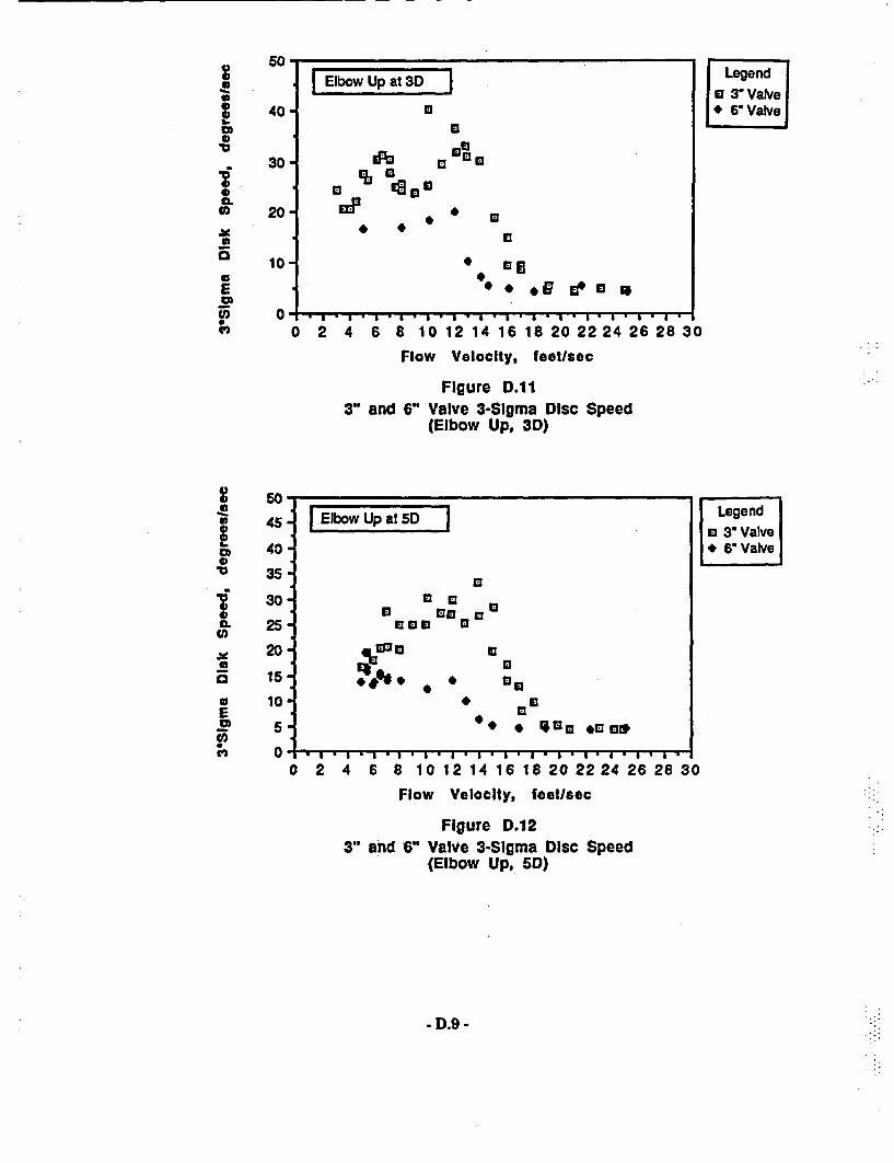
S

0.V

-Pa

;S

0

0)

00

a)

Ea

B

50

40

30

20

10

0

5045

40

35

30

25

20

15

10

5

0

IElbow Up at 3DI

B

va

MP *~~ #

*S *O G do 5 l

., ., ., ., ., ., ., .,.,.L0 2 4 6 8 10 12 14 16 18202224 26283C

Flow Velocity, feet/sec

Figure D.113" and 6" Valve 3-Sigma Disc Speed

(Elbow Up, 3D)

| Elbow Up at 5D | Legendm 3' Valve* 6" Valve

BU.M

0coo mea

*4 * 0 * so *ma

I0 2 4 6 8 10 12 14 16 18 20 22 24 26 28

Flow Velocity, feet/sec

Figure D.123" and 6" Valve 3-Slgma Disc Speed

(Elbow Up, 5D)

30

0

0

0

a.g2VS06

X0

21.

0

co

0

0.

0

16

14

12

10

8

6

4

2

0

16

14

12

10

8

6

4

2

0

13 low Downat OD

+4+4

3-*+~~~~~44

a 3 +

aa pU ea E

.* I ., ,, .I , I * , I , I I0 2 4 8 8 10 12 14 16 18 20 2224 26 28 30

Flow Velocity, feet/sec

Figure D.133" Valve Moan Disc Speed

(Elbow Down, OD)

1+ 73', stopI*630stopI

1+ 73"1 stopI*63*0stopI

30Elow onat1IDI

IPO +

**I4t.I + +

m * ~ 4

4.

0 2 4 6 8 10 12 14 18 18 20 22 24 28 28 30Flow Velocity, feet/sec

Figure D.143" Valve Mean Disc Speed

(Elbow Down, 1D)

-D.10-

m-e06

f(0

CO

(09

S

CSeW

12'-12 FElbow Down at 3D

10

+8-~~+4 + + +.

6- 1+ + , ++

4 - *C z +

2 la ++

+¢n n=*44+ +

0 1 0 2 0 3 0Flow Velocity, feet/sec

Figure D.153" Valve -Mean Disc Speed

(Elbow Down, 3D)

12-I Elbow Down at 5D I

10 F

,- +fi + +

U + 4.~~~

4 a 0 +

2 at0* p * -

O- 10. 20 3-.........

Legend+ 730stop* 63- stopa 530 stop

Legend+ 730 stop* 630 stopo 530 stop

0 2 4 6 8 10 12 14 16 18 20 22 24 26 28 30

Flow Velocity, feet/sec

Figure D.163" Valve Mean Dlsc Speed

(Elbow Down, SD)

- D.1 -

80 ~ ~ *Legend

* 7 16 Elbow Down atODI +70-stopIl

e+ + * 60- stop6 + + 50 stop

* +~~~~~~~~

.0i 4 e + + +0.* 4 - l +

3 + + +

o 2 v2

0

0 2 4 6 8 10 12 14 1618 20 22 24 28 28 30Flow Velocity, ftet/sec

Figure D.176" Valve Mean Disc Speed

(Elbow Down, OD)

<,6-e 1~~6- Elbow Down t 1 D Legen

[i~~~o~~~i~~ownat1D ~ ~ ~ ~ +700stop

5 stop

o 4. +

.0 1- 4 4. Z 4 >. Dr

O - 4 13 8 01 41 8202 42 83

0

Flow Velocity, feet/soc

Flgure D.186" Valve Mean-Disc Speed

(Elbow Down, ID)

-D.12-

0

0

04

00

An0

CL

0Ok

C

a

6

5

4

3

6 Ebw Downat 31)ID

m. a * ina Ma. a a U I

2

1

0

6

i I a I a * a * a * * X A I0 2 4 6 8 10 12 14 16 18 20

Flow Velocity, feet/sec

Figure D.196" Valve Mean Disc Speed

(Elbow Down, 3D)

Legend+ 700 stop* 600 stopl 50° stop

Legend+ 70° stop.* 60°stopn 50° stop

U

00

E

(In

CLW

0

5.

4.

3.

2-

I1-

16 Ebo own at 51)

a4.

+

4.4.

.4-

IF4+

- *a gb 8C

1 la 14 +Is

0 B - I -

0 2 4 6 8 10Flow Velocity,

12 14

feet/sec1 6 18 20

i Figure D.20t6" Valve Mean Dlscs Speed

(Elbow Down, 5D)

-D.13 -

0aSa

b.

0

0.

aa

CL

U)

0

I.

0

0.

CO

U)

(aCO)

60

50

40

30

20

10

0

60

50

40

30

20

10

0

I lbwaowta0 D IU U3

*3a

U

13 a

1% 0~~~S

113" ValveI

I3 3'Valve

1.1. I A I. aI&IIIII0 2 4 6 8 10 12 14 16 18 20 22 24 26 28 3C

Flow Velocity, feet/sec

Figure D.213" and 6" Valve 3-Sigma DIsc Speed

(Elbow Down, OD)

I lbwDown at D ID

U

Ur M

_%Y. 13 *U

I

.50O 2 . I f I f I . I . I I .B .1 .1 .1 .

2 4 6 8 10 12 14 16 IS 20 22.I. I I I I 1

24 26 28 30

Flow Velocity, feet/sec

Figure D.223" and 6" Valve 3-SIgma Disc Speed

(Elbow Down, ID)

-D.14-

a0a0C0

0

la

0I,

AC2aa

E0S

a

0

J9~

40

30

20-

10-

Elbow Down at 3Da

ae FP

m*UU00

a

U 0

aa C a aa 0

00

40

30

20

10

0

l' I a I a I a I a .a . I I ,., .I .I I li0 2 4 6 8 10 12 14 16 18 20 22 24 26 28 3C

Flow Velocity, feet/sec

Figure D.233" and 6" Valve 3-Sigma Disc Speed

(Elbow Down, 3D)

jDowDownaat5D I

a a aa

' *.* .. .* .* .* .-a. .................

J030 Valvej

Legendfa3' Valve~* G Vlv

0 2 4 6 8 10 12 14 16 18 20 22 24 26 28 30

Flow Velocity, feet/sec

Figure D.24

3" and 6" Valve 3-Slgma DIsc Speed(Elbow Down, SD)

-D.15-

300Sa

*0

a.

S

C*

a

a

aa0S

*0

0

00.

2

25

20

15

10

5

0

20

15

10

5

0

13/16- Holes Orifice at 1.5(

Fe* + +

.~~~~~~~~4Me. 4.+

El

In la 's*

l

0 2 4 6 8 10 12 14 16 18 20Flow Velocity, feet/sec

Figure D.253" Valve Mean Disc Speed

(3116" Holes, Orifice Plate at 1.5D)

17/8* Holes Orifice at 1.5DI

+° * a a a * +

+ +

I . I I4I I

I+73.VstopIIB83 stopI

1+ 73"1 stopI' 631 stop0 50tsop

0 2 4 6 8 10 12 14 16 18

Flow Velocity, feet/sec

Figure D.263"' Valve Mean Disc Speed

(7/8" Holes, Orifice Plate at 1.5D)

20

-D.16 -

30 I00

0

0ECa

8

0

I 13/8' Holes Orifice at 1.51

25-

20 -

15

10

:1 ,

Legend+ 700 stop* 60° stop0 501, stop

++

++

+

+4

C ++ *4'O:

* .a + d u~~ e~

I-. I�p*,*p*p�-i� -.

0I --I. a .0~~~~~~~~~~~~~~~~~~~ .a. I .I . I .I .

2 4 6 8 10 12 14 16 18

Flow Velocity, feet/sec

Figure D.276" Valve Mean Disc Speed

(3/8" Holes, Orifice Plate at 1.5D)

20

&' .'

a0a0,0

0

0.CD

m

C

01

15-

10 -

5-

11.75' Holes Orifice at 1.5DI

if ++4+I

%a

% G~ +

I+700stopI* 600stopI

, . . . . ~ 1

0 2 4 6 8 10 12 14 16 18

Flow Velocity, feet/sec

20

Figure D.286" Valve Mean Disc Speed

(1.75" Holes, Orifice Plate at 1.5D)

- D.17 -

0aa-Sao2IS

a

0

0

.9C.)

120110

100

8 10 12 14 16

Flow Velocity, feet/sec

Figure 0.296" Valve Mean Disc Speed

(3116" Holes, Orifice Plate at 1.50)

0aCs5-aaS

0.

a)a

0

10090 -

80 -

70 -

60 -

50-

40-

30 -

20 -

10-

0 -

I

70 Sto Orifice at 1 .5D

I Orifice at 1.51)

0

U o

009...*

."+4 03

I Legendl 318' Holes

* 1.7520Hole

2 0

U

.a 40

a ~ ~ . . . . . . .o . 2 I . 8 . I . 1 2 1 1 6 1 8 I

0 2 4 6 8 1 0 1 2 1 4 1 6 1 8

Flow Velocity, feet/sec

Figure D.306" Valve 3-Sigma Disc Speed

(Orifice Plate at 1.50)

-D.18-

25C00

0)

i

F

0

CL

-0

0

C

£0*

S

a

CD

01

1 3/18" Holes Orifice at 2.5D I+

20 -

15-

10 -

4.0'

0T +

13

4.

0

l

0 092

0o C s 1 0as

0

25

20

15

10

5

0

a I I I I .

0 2 4 6 8 10 12 14 16 18 2C

Flow Velocity, feet/sec

Figure D.313" Valve Mean Disc Speed

(3/16" Holes, Orifice Plate at 2.5D)

LegendT 730 stop* 63e stopo 53° stop

Legend+ 730 stop* 63 stop13 530 stop

| 7/8' Holes Orifice at 2.5D I

4T-

4.+ 4

1-,o #*

+4

a 4. +4.Cim £ *a a

U -T -U * a * I * a * I * I * I * … * I

0 2 4 6 8 10 12 14 16 18 20

Flow Velocity, feet/sec

Figure D.323" Valve Mean Disc Speed

(7/8" Holes, Orifice Plate at 2.5D)

-D.19 -

0Saa00

h.

m

0

00

a

Cai

12

10

8-

6-

4-

2-

3/80 Holes Orifice at 2.5D

U D d

Legend+ 70- stop* 600 stopa Sol, stop

00 2 4 6 8 10

Flow Velocity, feet/sec

Figure D.336" Valve Mean Disc Speed

(3/8" Holes, Orifice Plate at 2.5D)

00i010

-01

0.

0

as

Cai0

12

10

8

6

4

2

0

Legend+ 701 stop* 601 stopl 5011 stop

0 2 4 6 8 10 12 14 16

Flow Velocity, feet/sec

Figure D.346" Valve Mean Disc Speed

(1.75" Holes, Orlifce Plate at 2.5D)

18 20

- D.20-

0

0

0

b.0

0,

-i4)

0CLco00

a

S

E1R

100

90

80

70

60

50

40

30

20

10

0

100

90

80

70

60

50

40

30

20

10

0

I

Orfieat2.51)

0

IF

C0 0

* 0 0

*9 0 %?

I . -I A I I I a . . . .... . I0 2 4 6 8 10 12 -14 16 18 2C

Flow Velocity, feet/sec

Figure D.353" Valve 3-Sigma Disc Speed

(Orifice Plate at 2.5D)

I . *1

Legend

# 7/81 HolesI

j r 3/8" HolesL .7" olesj

I riice at 2.51)

0moEmm la0

10 0.

* * 0

I MO~~ 0 inU

0 2 4 6 8 10 12 14 16 18 20

Flow Velocity, feet/sec

Figure D.366" Valve 3-Sigma Disc Speed

(Orifice Plate at 2.5D)

*D.21 -

0a

00

-01

0)a

C.x

aa

0

00

a

0

0.1

Ca00

20311 6 Holes Orifice at 4.50

15 -9

El+

5 D +

0 2 4 6 8 10 12 14 18 18 20Flow Velocity, feet/see

Figure D.373" Valve Mean Disc Speed

(3/16" Holes, Orifice Plate at 4.5D)

20 -7/8B Holes Orifice at 4.50

15

10 - +* +~~ ~+4+

+ 4 + + +

5 +~~~~~~~ C ~ ~ ~

M13g * 0 lp *

0 2 4 6 8 10 12 14 16 18 2(

Legend+ 73e stop* 63e stopEl 530 StOp

Legend+ 73e stop* 630 stopD 53e StOp

)

Flow Velocity, feet/sea

Figure D.383" Valve Mean DIsc Speed

(7/8" Holes, Orifice Plate at 4.5D)

- D.2:2-

00-0a0E0*0

0

CLSx

20

is-

10 -

5-

| 3180 Holes Orifice at 4.5D I Legend+ 70O stop* 600 stopa 5V0 stop

04. + +

0 +++

4..~~~41

a *0 *a~5~O

a.60

C+

4.4.+

+$

is a4. +'m+1

0 'I

0 2 4 6 8 10 12 14 16 18 20

Flow Velocity, feet/sec

Figure D.396" Valve Mean Disc Speed

(318" Holes, Orifice Plate at 4.5D)

inC0-00

*0

0.

10

lef0L

01

8-

I

6-

4-

2 -

1 1.75 Holes Orifice at 4.51I

*

B +T

B 1B * + 4* 4

,'mm&. T a + m 0 4

n4.~ b. U B I

I+700stopl*00stop

L 50. stop

0 I...... . I. I I a ..... I. . I. ..... I . I- . I .A

0 2 4 6 8 10 12 14 16 18 20

Flow Velocity, feet/sec

Figure D.406" Valve Mean Disc Speed

(1.75" Holes, Orifice Plate at 2.5D)

-D.23-

0

0

S6

0.C*

0.Cl)

0

21

01

0

0.1Cl)

B;

50s

40

30

20

10

0

60

50

40

30

a a 3 1 rifie at 4.51)

0 * 0U0~~~~~

*~~~~~1

9 a

I

, I., ., . ., . I . I I0 2 4 6 8 10 12 14 16 18 2C

Flow Velocity, feet/3sc

Figure D.413" Valve 3-Sigma Disc Speed

(Orifice Plate at 4.5D)

a 3/1 6"Hates

1U7/8' HolesI

a /WHolesOrifice at 4.5D)

a amU

mm, V

U aN

13a *g~~U 5 *

20 -

10 -

0 .1--I . - - - - -~ ~~ . .E . ^ .

0I ' . a * a . I - , . a . .

2 4 6 8 10 12 14Flow Velocity, feet/sec

16 18 20

Figure D.426" Valve 3-Sigma Disc Speed

(Orifice Plate at 4.5D)

- D.24 -

a

U

I00

CLS)SK

6

| 3/16- Holes Orifice at 1 OD1-

0 + * .+

+ + ld5

* B

* 3

Legend

+ 730 stop* 630stopa 530 stop

4

0 '.u.

0 2 4 6 8 10

Flow Velocity, feet/sec

Iigure D.433" Valve Mean Disc Speed

(3/16" Holes, Orifice Plate at 10D)

S

0

U01

iSLS)

8

. 6

4

2

0

I+73-stopI1* 630 stop

20Flow Velocity, feet/sec

Figure D.443" Valve Mean DIsc Speed

(7/8" Holes, Orifice Plate at 10D)

-D.25 -

6a0

0

-01

-o

0.b

0

-a.

0

-01

0

0.

0

iS

5

4

3

2

1

0

5

. 318' Holes Orifice at 10D

l +

a *0

03 a Q * a* 0 0*

9 *~~ a & *

0 2 4 6 8 10

Flow VelocIty, feetlsec

Figure D.456" Valve Mean Disc Speed

(3/8" Holes, Orifice Plate at 1OD)

. -~~~~~~~~~~~~~~~~~~~

Legenct+ 70- stop* 60' stopo 50 stop

Legend+ 70' stop* 60' stop13 500 stop

3 -

2-

1-

1 1.75S Holes Orifice at 100D

++~~ ~~ U+~ a P +

Ul

q . . . . . . . . . _

0I . I . - U- --.

2 4 S 8 102I- 1- 16 1

1 2 14 16 18 20

Flow velocity, leetlsec

Figure D.466" Valve Mean Disc Speed

(1.75" Holes, Orifice Plate at 10D)

- D.26 -

a)0

000

S

0

1.9

-0

10

9..

8

7.

6-

5.

4.

3.

2-

1*n .

9

0~~~~~~a 0

a1U

A

j0n3/16' Holes* 78' oles

16 16 2U . .. . .. . ..U -.............

0 2 4 6 8 10 12 14Flow Velocity, feet/sec

Figure D.473" Valve 3-Sigma Disc .Speed

(Orifice Plate at 10D)

S

06S.1

C.0

SW

0

E0

24222018161412

10 -

6-

42-0 :

I Orifice at 10D

0 0 d 0 Ed 0

0 * EU

& a * .

LegedIU3/8SHolesI[ 175*Hole

-- - -Ir

0 2 4 6 8 10 12Flow Velocity, feet/sec

Figure D.486" Valve 3-Sigma Disc Speed

(Orifice Plate at 10D)

- D27 -

3" 300 lb Swing Check Valve

100_ * ~~~~~~~~~~~~Strong Turbulence

80- 0 WekTublecX * X * 1|1 ~~~~~~~~~Elbow Up

ffi 60 - + | | | ES}~~ Elbow Down~60

j 40-

E20

Lw, 0

OD 10-1.5D 2.5D-3D 4.50-50 IODUpstream Distance to Disturbance

Figure D.493-inch Valve: Relative Severity of Various Upstream Disturbances

Expressed In Terms of 3 Sigma Disc Speed

6" 300 lb Swing Check Valve

100_ * ~~~~~~~~~~~~Strong Turbulence

so 8- M eakTuzteX~~~~~~~~~~~~ Eb w EUp

~40-

220

OD 1 D-1.5D 2.5D-3D 4.5D-5D 1ODUpstream Distance to Disturbance

Figure 0.506-Inch Valve: Relative Severity of Various Upstream Disturbances

Expressed In Terms of 3 Sigma Disc Speed

- D.28 -

NRC FORM 335 US. NUCLEAR REGULATORY COMMISSION 1. REPORT NUMBER12-89) = ige b NFC. Add Vol.. e~ eNRCM 110:2 C VW tdm tnbma. Io V.3201.3M BIBLIOGRAPHIC DATA SHEET

(See iflstfucti -on nndI ~NUREG/CR-55832. TITLE AND SUBTITLE KEI No. 1656

Prediction of Check Valve Performance and Degradation in 3. DATE REPORTPUBLISHED

Nuclear Power Plant Systems -- Wear and Impact Tests 3. j VYEAR

August 19904. FIN OR GRANT NUMBER

X________________________________ _ -D2510S. AUTHOR (S) S. TYPE OF REPORT

Technical7. PERIOD COVEREDIm*cAu gs;

M.S. Kalsi, C.L. Horst, J.K. Wang, V. Sharma 9/88 - 4/90

L. MrcnRvING'4 unuRGuAIZAHO - NAME~ PIU MULFwncaz Or ~L v.WW.U~ ff~g4I. I&M -- VWMSWY~l,, W 5' ~ Psmea and ffWeflln .d~id.

Kalsi Engineering, Inc.745 Park Two DriveSugar Land, Texas 77478

P. SPONSORING ORGANIZATION-NAME AND ADDRESS ifN. type- .me o.wioN to.pvid RCivbion. Office as, ReoCgion. U.& NchaeRguAtorC.mmsln.and w eddmm)

Division of EngineeringOffice of Nuclear Regulatory ResearchU.S. Nuclear Regulatory CommissionWashington, DC 20555

10. SUPPLEMENTARY NOTES

11. ABSTRACT 10 0wo.'o ai

Check valve failures in nuclear power plants have led to safety concerns as well asextensive damage and loss of plant availability in recent years. Swing check valveinternals may experience premature degradation if the disc is not firmly held openagainst its stop and significant flow disturbances are present upstream within 10 pipediameters. The objective of the current Phase II research was to develop and experi-mentally verify a quantitative methodology for predicting swing check valve performanceand the degradation of internals caused by hinge pin wear or disc stud impact. Phase Iresearch had focussed on investigating the stability of the swing check valve disc atdifferent flow velocities for a wide variety of upstream flow disturbances locatedwithin 10 pipe diameters of the check valve. Valve performance predictions based onmethodology developed as a result of Phase I and II research correlate well with actualvalve operating history at plants. The conservative guidelines provided by thismethodology, tempered and refined by actual performance history and integrated withpreventive maintenance activities, have the potential for significantly improving theoverall reliability of check valves in nuclear power plants.

12. KEY WORDS/DESCRIPTORS sartwo and ophmm shot wil henw&e*s hi csdnu m tpwr.i t o AVAIABILITY STATEMENT

check valve behavior Unlimitedcheck valve degradation 14. SECURITY CLA3SIFICATIO

aging research rr ")wear and impact on check valves Unclassified

Ih X4gf.

Unclassified5. NUMBER OF PAGES

16. PRICE

kRC FORM 335 42491

UNITED STATESNUCLEAR REGULATORY COMMISSION

WASHINGTON, D.C. 20555

OFFICIAL BUSINESSPENALTY FOR PRIVATE USE, $300

FOUIL XRTH-CLASS RATESPOSTAGE & FEES PAID

AMNoC

PERMITNo. G J6