Numerical  Methods  in    Biomedical  Engineering  

Lecture’s  website  for  updates  on  lecture  materials:  h5p://9nyurl.com/m4frahb  

     Individual  and  group  homework       Individual  and  group  midterm  and  final  projects       (Op?onal)  computer  lab  every  Monday,  Room    B03,  5-­‐6.30pm    

What  are  numerical  methods?  Techniques  by  which  mathema?cal  problems  are    

formulated  so  that  they  can  be  solved    with  arithme?c  opera?ons.  

They  provide  approxima?ons  to    the  problems  in  ques?on.  

Why  study  numerical  methods?  

Most  (  >  99.9%)  of  real  world  problems  in  science  and  engineering  are  too  complex  and  sophis?cated  to  be  

solved  analy?cally  (exactly),  hence  they  can  only  be  solved  numerically  (approximately).  

[Computa?onal  Modeling  of  Endovascular  Deep  Brain  Simula?on]  hXps://www.msi.umn.edu/content/computa?onal-­‐modeling-­‐endovascular-­‐deep-­‐brain-­‐simula?on  

Errors  and  Numerical  Series  

Errors  •  Computers use a base-2 representation

1 0 1 0 1 1 0 1

•  Computers cannot precisely represent certain exact base-10 numbers. Non-integer numbers, such as π = 3.1415926535…, e = 2.718281…, or are cumbersome and can’t be expressed by a fixed number of significant figures.

•  The discrepancy creates an error usually referred to as round-off error or rounding error

Errors  Suppose ã is an approximation to the (nonzero) true value a, then:

Absolute error

Relative error

Example: the value of π = 3.1415926535… is to be stored on a base-10 system that allows 7 significant figures. Chopping approximation π = 3.141592 Absolute error = |3.1415926535 – 3.141592| = 0.0000006535 Rounding approximation π = 3.141593 Absolute error = |3.1415926535 – 3.141593| = 0.0000003465

Floa9ng-­‐point  System  Fractional numbers in computers are usually represented using floating-point form:

man?ssa  base  of  the  number  system  being  used  

exponent  

Example: in a floating-point base-10 system that allows only 4 decimal places to be stored, the quantity 1/34 = 0.029411765 would be stored as 0.2941 x 10-1

Allows both fractions and very large numbers to be expressed on the computer

Takes up more space Takes longer time to process Source of round-off error

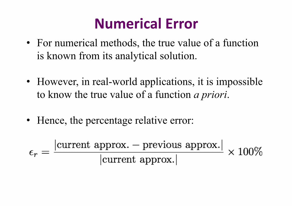
Numerical  Error  •  For numerical methods, the true value of a function is known from its analytical solution.

•  However, in real-world applications, it is impossible to know the true value of a function a priori.

•  Hence, the percentage relative error:

Maclaurin’s  series  

Let the power series for f(x) be

where are constants.

At

Substituting for in f(x) gives:

Condi9ons  of  Maclaurin’s  series  

(3) The resultant Maclaurin’s series must be convergent

0  

f(0)  f(h)  

x  

y=f(x)  

y  

h  

P  

Q  

Using Maclaurin’s series, at some point Q in Figure above:

Taylor  series  If the y-axis and origin are moved a units to the left, the equation of the same curve relative to the new axis becomes y = f(a+x) and the function value at P is f(a).

0  

f(0)  

f(a+h)  

x  

y=f(a+x)  y  

a  

P  

Q  

At point Q:

f(a)  

h  

Zero  order  

Taylor series provides a means to predict a function value at one point in terms of the function value and its derivatives at another point:

where:

n = order of derivative

Example  Use zero-through third-order Taylor series expansion to predict for

using a base point at . Compute the true percent relative error for each approximation. Solution The true value of the function at is , which is the value that we are going to predict/approximate.

For , the Taylor series approximation is

and relative error

For , the first derivative is , and the first order Taylor series approximation

For , the second derivative is , and the second order Taylor series approximation

and relative error

and relative error

For , the third derivative is , and the third order Taylor series approximation

hence, the remainder term is

The Taylor series expansion to the third order derivative yields an exact estimate at ,

Trunca9on  Errors  Taylor series can be used to estimate truncation errors.

The notion of truncation errors usually refers to errors introduced when a more complicated mathematical expression is “replaced” with a more elementary formula.

From the Taylor series expansion

we truncate the series after the first derivative term

Trunca9on  Errors  

Using

for , we get

or

Rearranging the equation gives us

trunca?on  error  first-­‐order  approxima?on  

Error  Propaga9on  

The problem with evaluating is that f(x) is unknown because x is unknown. We can overcome this if: •  is close to x, and •  is continuous and differentiable

We use Taylor series to compute f(x) near

Suppose we have a function f(x) which has one dependent variable x. Assume that is an approximation of x. To assess the effect of the discrepancy between x and on the value of the function, we use

Error  Propaga9on  

where

or

Dropping the second- and higher-order terms and rearranging gives us

represents an estimate of the error of the function f(x) represents an estimate of the error of x

This enables us to approximate the error in f(x) given the derivative of a function and an estimate of the error in x.

Taylor  Series  for  Func9ons  with  More  than  One  Variable  

If we have a function of two independent variables x and z, the Taylor series can be written as

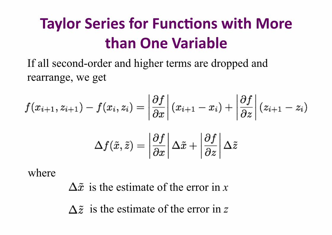
Taylor  Series  for  Func9ons  with  More  than  One  Variable  

If all second-order and higher terms are dropped and rearrange, we get

where is the estimate of the error in x

is the estimate of the error in z