NumericalAnalysis-AnIntroduction … · we try to minimize by using MATLAB as a toolbox for...
136
Numerical Analysis - An Introduction Claus F¨ uhrer, Achim Schroll Numerical Analysis Center for Mathematical Sciences Lund University 3 rd Edition, 2001
-
Upload
truongkiet -
Category
Documents
-
view
223 -
download
7
Transcript of NumericalAnalysis-AnIntroduction … · we try to minimize by using MATLAB as a toolbox for...

Numerical Analysis - An Introduction
Claus Fuhrer, Achim SchrollNumerical Analysis
Center for Mathematical SciencesLund University
3rd Edition, 2001

ii
Contents
1 Interpolation and Curve Design 1
1.1 Some Definitions and Notations . . . . . . . . . . . . . . . . . . . 1
1.2 Polynomial Spaces and Interpolation . . . . . . . . . . . . . . . . 3
1.2.1 Lagrange Polynomials . . . . . . . . . . . . . . . . . . . . 5
1.2.2 Newton Interpolation Polynomials. . . . . . . . . . . . . . 6
1.2.3 Interpolation Error. . . . . . . . . . . . . . . . . . . . . . . 8
1.2.4 Polynomial Interpolation in MATLAB . . . . . . . . . . . 10
1.2.5 Bernstein Polynomials . . . . . . . . . . . . . . . . . . . . 11
1.3 Bezier Curves . . . . . . . . . . . . . . . . . . . . . . . . . . . . . 13
1.3.1 Some notations and definitions . . . . . . . . . . . . . . . 13
1.3.2 de Casteljau Agorithm . . . . . . . . . . . . . . . . . . . . 15
1.3.3 Bezier curves and Bernstein polynomials . . . . . . . . . . 17
1.3.4 Chebyshev Polynomials . . . . . . . . . . . . . . . . . . . 19
1.3.5 Three-term recursion and orthogonal polynomials . . . . . 23
1.4 Quadrature formulas . . . . . . . . . . . . . . . . . . . . . . . . . 26
1.4.1 Quadrature in MATLAB . . . . . . . . . . . . . . . . . . . 29
1.4.2 Gauss Quadrature . . . . . . . . . . . . . . . . . . . . . . 29
1.5 Piecewise Polynomials and Splines . . . . . . . . . . . . . . . . . . 32
1.5.1 Minimal Property of Cubic Splines . . . . . . . . . . . . . 35
1.5.2 B-Splines . . . . . . . . . . . . . . . . . . . . . . . . . . . 36
2 Linear Systems 41
2.1 Regular Linear Systems . . . . . . . . . . . . . . . . . . . . . . . 42
2.1.1 LU Decomposition . . . . . . . . . . . . . . . . . . . . . . 42
2.1.2 Matrix Norms, Inner Products and Condition Numbers . . 48
2.2 Nonsquare Linear Systems . . . . . . . . . . . . . . . . . . . . . . 52
2.2.1 Projections . . . . . . . . . . . . . . . . . . . . . . . . . . 54
2.2.2 Condition of Least Squares Problems . . . . . . . . . . . . 55
2.2.3 Orthogonal factorizations . . . . . . . . . . . . . . . . . . 56
2.2.4 Householder Reflections and Givens Rotations . . . . . . . 58
2.2.5 Rank Deficient Least Squares Problems . . . . . . . . . . . 60
iii
iv CONTENTS
3 Signal Processing 633.1 Discrete Fourier Transformation . . . . . . . . . . . . . . . . . . . 63
4 Iterative Methods 734.1 Computation of Eigenvalues . . . . . . . . . . . . . . . . . . . . . 74
4.1.1 Power iteration . . . . . . . . . . . . . . . . . . . . . . . . 754.2 Fixed Point Iteration . . . . . . . . . . . . . . . . . . . . . . . . . 784.3 Newton’s Method . . . . . . . . . . . . . . . . . . . . . . . . . . . 82
4.3.1 Numerical Computation of Jacobians . . . . . . . . . . . . 844.3.2 Simplified Newton Method . . . . . . . . . . . . . . . . . . 85
4.4 Continuation Methods in Equilibrium Computation . . . . . . . . 874.5 Gauß-Newton method . . . . . . . . . . . . . . . . . . . . . . . . 914.6 Iterative Methods for Linear Systems . . . . . . . . . . . . . . . . 92
5 Ordinary Differential Equations 955.1 Differential Equations of Higher Order . . . . . . . . . . . . . . . 965.2 The Explicit Euler Method . . . . . . . . . . . . . . . . . . . . . . 96
5.2.1 Derivation of the Explicit Euler Method . . . . . . . . . . 975.2.2 Graphical Illustration of the Explicit Euler Method . . . . 975.2.3 Two Alternatives to Derive Euler’s Method . . . . . . . . . 985.2.4 Testing Euler’s Method . . . . . . . . . . . . . . . . . . . . 99
5.3 Stability Analysis . . . . . . . . . . . . . . . . . . . . . . . . . . . 1005.4 Local, Global Errors and Convergence . . . . . . . . . . . . . . . 1015.5 Stiffness . . . . . . . . . . . . . . . . . . . . . . . . . . . . . . . . 1035.6 The Implicit Euler Method . . . . . . . . . . . . . . . . . . . . . . 104
5.6.1 Graphical Illustration of the Implicit Euler Scheme . . . . 1065.6.2 Stability Analysis . . . . . . . . . . . . . . . . . . . . . . . 1065.6.3 Testing the Implicit Euler Method . . . . . . . . . . . . . . 107
5.7 Multistep Methods . . . . . . . . . . . . . . . . . . . . . . . . . . 1095.7.1 Adams Methods . . . . . . . . . . . . . . . . . . . . . . . . 1095.7.2 Backward Differentiation Formulas (BDF) . . . . . . . . . 1125.7.3 Solving the Corrector Equations . . . . . . . . . . . . . . 1135.7.4 Order Selection and Starting a Multistep Method . . . . . 114
5.8 Explicit Runge–Kutta Methods . . . . . . . . . . . . . . . . . . . 1155.8.1 The Order of a Runge–Kutta Method . . . . . . . . . . . . 1175.8.2 Embedded Methods for Error Estimation . . . . . . . . . . 1185.8.3 Stability of Runge–Kutta Methods . . . . . . . . . . . . . 120
PrefaceThe basic education in mathematics at LTH ends with an introductory coursein Numerical Analysis. Many mathematical problems have been introduced andmethods to solve some of them exactly (or analytically) have been studied. Sincecenturies mathematics was focused on finding exact solutions to mathematicallyformulated problems in science and engineering. With the appearance of firstmechanical and then electronic computing devices the interest in approximatesolutions to problems which could not be solved exactly increased drasticallyand so-called numerical methods were developed. ”Numerical” means in thatcontext that already in an early stage mathematical manipulation of algebraicexpressions are replaced by computations with numbers. A function is replacedby an algorithm, which evaluates the function for a given numeric argument.In this introduction course we will present some of the most important computa-tional methods and we will analyze them, to see how accurate results they maygenerate and how robust. That’s why the course is called Numerical Analysis.The numerical part will demand from you some skills in programming, whichwe try to minimize by using MATLAB as a toolbox for performing numericalexperiments. In this part you will miss the classical ”paper-and-pencil” way towork in mathematics. The analysis part demands good knowledge in calculus andlinear algebra. Finally the course has a strong engineering science part where welink the field to important problems in applications.The lecture notes (this booklet) covers the analytical part. We tried to use amathematical language and avoid to present the material just by a collectionof ”recipes”. The collection of computer assignments and also the final projectrelated exam covers the algorithmic and engineering part. All three parts areimportant and interact permanently.Though we try to motivate all methods by practical examples, their importanceof some techniques might become clear for you in later stages in your engineeringeducation.This course starts a series of other courses in numerical analysis on a more ad-vanced level. It should also be completed by courses in applied mathematics,signal processing and control theory.Be aware that lecture notes are no textbook. Therefore you will find referencesto other literature in the text. It will help you a lot, if you look at some of thesereferences and also classical textbooks.
Claus Fuhrer & Achim Schroll, Lund, October 2001
v

vi CONTENTS

Notational conventions
In this manuscript we apply (hopefully consequently) the following conventions
• indices, integer numbers: small Latin letters in the range [i − n], see For-tran60 convention.
• scalar numbers: Greek letters, e.g. α, β, . . .
• vectors: small Latin letters mainly from the end of the alphabet, e.g.u, v, w
• matrices: capital Latin letters, e.g. A,B, . . .
• identity and zero matrix: I and 0 (sometimes with the dimension as asubscript).
• matrix elements Aij or ai,j
• linear spaces: caligraphic letters, e.g. C• norms: ‖ · ‖ with the type of norm as subscript (if necessary)
• absolute value (modulus): | · |
vii

viii CONTENTS

Topics
Course hoursPolynomial Interpolation all 4Bezier Curves D 2Spline Interpolation all 4Bezier Splines D 2Norms, Stability, Condition all 2Linear Systems of Equations all 2Least Squares (Data fitting) all 2Orthogonal Factorization I 2Numerical Signal Processing: FFT all 4Nonlinear Systems: Fixed point problems all 2Nonlinear Systems: Newton Iteration all 2Nonlinear Data Fitting: Gauss-Newton I 2Ordinary Differential Equation: Initial Value Problems all 8Ordinary Differential Equations: Boundary Value Problems F,I,K 4Basics of Parameter Estimation I 2
ix

x CONTENTS

Chapter 1
Interpolation and Curve Design
Before reading this paragraph make sure, that you are familiar with the basicsin Linear Algebra. Reread Chapter 6.2 in [Spa94].
1.1 Some Definitions and Notations
Interpolation Interpolating data is one of the most important topics in NA.It is used to obtain a “handy” functional description instead of just the raw dataobtained from measurements, observations etc.A functional description has several purposes:
• Compressing the amount of data
• Give information about values not covered by measurements, i.e. interpo-lation, extrapolation
• Speed up evaluation: function evaluation is often faster than table-look-ups
On the other hand interpolation is also the basis of many other more advancedmethods in NA.The situation is the following:
Definition 1Given data points (ti, yi), i = 1, . . . , n.A function f is called interpolating these data if
f(ti) = yi
You might think of the independent variable ti being time points while yi denotemeasurements at the these points.Other examples are pressure versus temperature, current versus voltage etc.There can be more measurements at a given time ti, thus yi might be a vectorwith several components.
1

2 CHAPTER 1. INTERPOLATION AND CURVE DESIGN
An interpolating function (or an interpolant) is seeked often in the set of poly-nomials, piecewise polynomials, trigonometric polynomials, rational functions orpiecewise rational functions. In this course we will not treat interpolation byrational and piecewise rational functions.Sometimes the requirements for interpolation are giving more restrictions on thefunction than desired. If we relax the interpolation by asking for the residuals
f(ti)− yi = ri
being small or even minimal in some sense, than we speak about approximationinstead of interpolation. For this end we have to discuss what we mean by “small”or “minimal” and we have to introduce norms and inner products. This will bethe topic in a later chapter.Another important topic in this context is curve design. Curve design is the taskcovered by many modern drawing programs like FREEHAND, COREL DRAWetc. It is also the basis for font generation for example in METAFONT and inthe POSTSCRIPT language.
Parametric and Non Parametric Curves, Graphs Functions relate in aunique way independent variables t to dependent variables y ∈ R
n.The graph of a function is the set
Γf := {(
tf(t)
)|t ∈ [t0, te]}
and (ti
f(ti)
)is a particular point of that graph. Note, that the independent variable t isalways the first component of the points if we consider a graph of a function. tparameterizes the graph and the resulting curve is called a non parametric curve.
General curves are parametric, i.e. the describing parameter has to be givenseparately and is not a component of the points. The graph of a parametric2D-curve has the form:
Γ := {(f1(t)f2(t)
)|t ∈ [t0, te]}
where f1 and f2 are functions over the given interval. A given graph can havedifferent parameterizations, i.e.
Γ := {(f1(t)f2(t)
)|t ∈ [t0, te]} = {
(ϕ1(τ)ϕ2(τ)
)|τ ∈ [τ0, τe]}.

1.2. POLYNOMIAL SPACES AND INTERPOLATION 3
An example for graph of a non parametric curve is the plot of the sine function,while the plot of the letter ”S” in a given font is an example for a parametriccurve.In this curse we will consider only 2D-graphs together with interpolation, approx-imation and curve design.
1.2 Polynomial Spaces and Interpolation
We call a function
p(t) = antn + an−1t
n−1 + ...+ a1t+ a0 (1.1)
a polynomial of degree n. The ai ∈ Rk are its coefficients. Mostly we will consider
scalar polynomials, i.e. k = 1.The set of all nth degree polynomials is denoted by Pn.We note, that Pn is a linear space over R, which has dimension n+ 1.A basis can easily be given
Theorem 2 The monomials 1, t, t2, . . . , tn form a basis of Pn.While uniquely defining a general function we need infinitely many values (allfunction values), a polynomial is uniquely given by n + 1 coefficients. Thus acommon task in Numerical Analysis is to approximate a given function by apolynomial and then describing it by its coefficients.We turn now to the interpolation task, which asks us to determine coefficients aiof a polynomial p(t) which interpolates the points (tj, yj), j = 0, . . . , k. Just bycomparing the amount of information we got with the number of unknowns weassume that we have to seek for a polynomial of degree n = k.Writing down the interpolation conditions
p(ti) = yi (1.2)
and rearranging the equations in matrix-vector form we obtain a square linearsystem of equations:
tn0 tn−10 · · · t0 1
tn1 tn−11 · · · t1 1· · ·
tnn tn−1n · · · tn 1
︸ ︷︷ ︸
=:A
an
an−1...a0
︸ ︷︷ ︸
=:x
=
y0y1...yn
︸ ︷︷ ︸
=:b
(1.3)
which has to be solved for the unknown coefficients ai.We will learn later in this course (cf. Ch. 2) how algorithms for solving thesekind of systems are constructed. Here we just take the corresponding MATLABcommand:

4 CHAPTER 1. INTERPOLATION AND CURVE DESIGN
x = A \ b
and find the ai as components of the solution vector x.The interesting question in this context is the solvability of the system, which isanswered by the following
Theorem 3 (Unisolvence Theorem)Given n+ 1 data points (ti, yi) with mutually different ti, there is a unique poly-nomial p ∈ Pn of (max) degree n which solves the interpolation task
p(ti) = yi i = 0, . . . , n
(The proof is based on contradiction).Thus we have to require, that we got measurements at distinct time points ti forobtaining a unique solution. In that case the matrix A is regular and the linearsystem has a unique solution.
Definition 4 The coefficient matrix
A :=
tn0 tn−1
0 · · · t0 1tn1 tn−1
1 · · · t1 1· · ·
tnn tn−1n · · · tn 1
of the linear system is called a Vandermonde matrix. 1
This matrix can be generated in MATLAB by the command vander.MATLABOnce the coefficients ai determined we can evaluate the polynomial at differentpoints. The cheapest way of evaluating is to apply Horner’s rule, which some-times also is called method of nested multiplications. For this end we rewrite thepolynomial in the following form:
p(t) =( · · · ((ant+ an−1)t+ an−2)t+ · · · a1
)t+ a0.
To evaluate p by using this formula requires n multiplications, while evaluatingthe polynomial in its standard form would require n(n+ 1)/2 multiplications.While determining an interpolation polynomial using monomials and solving theVandermonde system is quite easy it is numerically not the best thing to do. Theentries of that matrix might differ widely in magnitude already for rather smalln which leads to a badly scaled matrix and a lot of input information might belost during the process of solving this system. Furthermore adding (or removing)measurements require that the entire solution process has to be redone, whichmight be in same applications even for small n computationally to expensive.So we have to answer now two questions:
1For biographical notes on most of the mathematicians named in this manuscript checkhttp://www-groups.dcs.st-and.ac.uk/history/Mathematicians

1.2. POLYNOMIAL SPACES AND INTERPOLATION 5
• Are there alternative basis representations of Pn which allow us to computethe coefficients in a cheaper and more robust way?
• What is the typical degree of interpolation polynomials we have to dealwith?
Answering the first question leads us to the Lagrange and Newton basis of Pn.
1.2.1 Lagrange Polynomials
Let us consider a generic interpolation task and seek a polynomial interpolatingthe data for a given value j ∈ {0, . . . , n}
(ti, δij) with δij =
{0 for j �= i1 for j = i
Kronecker symbol
with i = 0 : n.It can be easily checked that the polynomial
Lnj (t) =n∏
i = 0i �= j
(t− ti)
(tj − ti)(1.4)
performs this task.
Example 5 For n = 2 the Lagrange polynomials are
L20(t) =
(t− t1)
(t0 − t1)
(t− t2)
(t0 − t2)
L21(t) =
(t− t0)
(t1 − t0)
(t− t2)
(t1 − t2)
L22(t) =
(t− t0)
(t2 − t0)
(t− t1)
(t2 − t1).
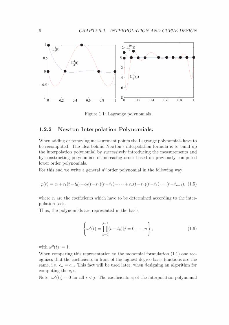
For n = 4 and n = 10 some Lagrange polynomials are depicted in Fig. 1.1
Definition 6 The n + 1 polynomials Lnj ∈ Pn, j = 0, . . . , n are called Lagrangepolynomials.
Theorem 7 The n+ 1 Lagrange polynomials form a basis of Pn.These polynomials are constructed in such a way, that the interpolation task canbe solved without solving any linear system. The interpolation polynomial is justa linear combination of the Lagrange polynomials with the measurements yi’s asfactors:
p(t) =n∑i=0
yiLni (t)
(Check, that p indeed interpolates the data!)
6 CHAPTER 1. INTERPOLATION AND CURVE DESIGN
� ��� ��� ��� ��� ���
���
�
��
�����
����
� ��� ��� ��� ��� ���
��
��
��
�
� �����
�����
Figure 1.1: Lagrange polynomials
1.2.2 Newton Interpolation Polynomials.
When adding or removing measurement points the Lagrange polynomials have tobe recomputed. The idea behind Newton’s interpolation formula is to build upthe interpolation polynomial by successively introducing the measurements andby constructing polynomials of increasing order based on previously computedlower order polynomials.
For this end we write a general nthorder polynomial in the following way
p(t) = c0+c1(t− t0)+c2(t− t0)(t− t1)+ · · ·+cn(t− t0)(t− t1) · · · (t− tn−1), (1.5)
where ci are the coefficients which have to be determined according to the inter-polation task.
Thus, the polynomials are represented in the basis
{ωj(t) =
j−1∏k=0
(t− tk)|j = 0, . . . , n
}, (1.6)
with ω0(t) := 1.
When comparing this representation to the monomial formulation (1.1) one rec-ognizes that the coefficients in front of the highest degree basis functions are thesame, i.e. cn = an. This fact will be used later, when designing an algorithm forcomputing the ci’s.
Note: ωj(ti) = 0 for all i < j. The coefficients ci of the interpolation polynomial

1.2. POLYNOMIAL SPACES AND INTERPOLATION 7
are then given as the solution of the following lower triangular system
ω0(t0) 0 0 · · · 0 0ω0(t1) ω1(t1) 0 · · · 0 0ω0(t2) ω1(t2) ω2(t2) · · · 0 0
...ω0(tn−1) ω1(tn−1) ω2(tn−1) · · · ωn−1(tn−1) 0ω0(tn) ω1(tn) ω2(tn) · · · ωn−1(tn) ωn(tn)
c0c1c2...
cn−1
cn
=
y0y1y2...
yn−1
yn
(1.7)
Such a triangular system can be solved by an easy recursion formula:
• Solve the first equation for c0
• Use this value and solve the next equation for c1
• and so on.
This recursive procedure can also be expressed in a recursion of successive inter-polation polynomials:Let us assume that pj−1 ∈ Pj−1 interpolates the first j data points. Then thepolynomial which interpolates the first j + 1 data points takes the form
pj(t) = pj−1(t) + cjωj(t). (1.8)
From the jth row in Eq. (1.7) one concludes
cj =yj − pj−1(tj)
ωj(tj)
This can be generalized to the composition of two interpolation polynomials oforder j − 1 two one of order j:
Theorem 8 (Lemma of Aitken)Let us denote by p(f |t1, . . . , tj) ∈ Pj−1 the polynomial which interpolates ti, yi :=f(ti), i = 1, . . . , j.Then the polynomial which interpolates ti, yi := f(ti), i = 0, . . . , j is given by
p(f |t0, . . . , tj)(t) =
(t0 − t)p(f |t1, . . . , tj)(t)− (tj − t)p(f |t0, . . . , tj−1)(t)t0 − tj
Definition 9 We denote by p(f |t0, . . . , tj−1) ∈ Pj−1 the polynomial which inter-polates ti, yi := f(ti), i = 0, . . . , j − 1.

8 CHAPTER 1. INTERPOLATION AND CURVE DESIGN
Its leading coefficient, i.e. the coefficient in front of tj−1 in its monomial repre-sentation is correspondingly denoted by
f [t0, . . . , tj−1].
These coefficients are called divided differences.
Note, by this definition f [ti] = f(ti).
An ultimate consequence of Aitken’s Lemma (Th. 8) is the recursion formula forthe divided differences, which is also the reason for their name:
f [t0, . . . , tj] =f [t1, . . . , tj]− f [t0, . . . , tj−1]
tj − t0. (1.9)
Furthermore we conclude from Eq. (1.8)
p(f |t0, . . . , tj)(t) = f [t0]ω0(t) + f [t0, t1]ω
1(t) + . . .+ f [t0, . . . , tj]ωj(t). (1.10)
Thus the coefficients cj of the interpolation polynomial are given by the divideddifferences, which can easily be computed recursively:
k = 0 k = 1 k = 2 . . . k = nt0 f [t0]
f [t0, t1]t1 f [t1] f [t0, t1, t2]
f [t1, t2]. . .
t2 f [t2]... f [t0, . . . , tn]
... f [tn−2, tn−1, tn]...
...f [tn−1, tn]
tn f [tn]
Note, the MATLAB command diff is a useful tool for forming differences ofvector components.MATLAB
1.2.3 Interpolation Error.
When interpolating a function we are often interested to estimate the interpola-tion error, i.e. the quantity
r(t) := f(t)− p(f |t0, . . . , tn)(t).

1.2. POLYNOMIAL SPACES AND INTERPOLATION 9
Theorem 10 Let f ∈ Cn+1(a, b) and let p(f |t0, . . . , tn) be the polynomial interpo-lating the points (ti, f(ti)), i = 0, . . . , n and denote by I(t0, . . . , tn, t) the smallestinterval containing t0, . . . , tn and t.Then there exists for all t ∈ (a, b) a ξ ∈ I(t0, . . . , tn, t) such that
r(t) =1
(n+ 1)!f (n+1)(ξ)ωn+1(t) (1.11)
holds.
Before we prove this theorem we discuss its consequences. The error is essentiallycomposed by two components, one depending on the function f and anotherdepending on ω(t) and consequently on the location of the ti and t. If the functionf and the polynomial degree is given, the only parameter which can be influencedto decrease the error is the location of ti. An equidistant grid of ti’s is not optimal.An optimal placing of the interpolation points will be discussed in the advancedcourse, when Chebychev polynomials are introduced.If t is outside I(t0, . . . , tn) we speak about extrapolation. Extrapolation is of-ten used for predicting the behavior of a process, e.g. the development of aninvestment fond. As can be seen from the exercise the Newton interpolationpolynomials and with them the interpolation error grow rapidly outside the datainterval. Extrapolation is therefore a numerically dangerous process.Proof (of Theorem 10):We fix a t �= ti and set F (t) := r(t)−Kωn+1(t) and determine K so that F (t) = 0.Then, F has at least n+2 zeros in I[t0, t1, . . . , tn, t]. Thus, by Rolle’s theorem F ′
has at least n + 1 zeros, F ′′ has n zeros and finally F (n+1) has at least one zero,say ξ ∈ I[t0, t1, . . . , tn, t].As p(n+1) ≡ 0 it follows
F (n+1)(ξ) = f (n+1)(ξ)−K(n+ 1)! = 0
Thus
K =f (n+1)(ξ)
(n+ 1)!
from which we obtain the expression for the error. ✷.So far we were interested in the error committed when interpolating a functionf by a polynomial of fixed degree. Can we decrease the error by increasing thedegree of the polynomials by adding more and more interpolation points?This question is discussed in the exercises (see Runge’s phenomenon), from whichwe conclude, that interpolation with high degree polynomials can lead to anhighly oscillatory error behavior and large errors.
Example 11 Assume the sine-function in [0, π/2] is interpolated by a fifth-orderpolynomial p on an equidistant grid. What is the upper bound for

10 CHAPTER 1. INTERPOLATION AND CURVE DESIGN
• the error at t = 0.1
• the error at t = 34π (extrapolation!)
• the maximal error in the interval [0, π/2]?The answers can be given directly by evaluating (1.11). Using the fact sin6(t) ≤ 1we can answer the questions by
• r(0.1) ≤ 1720
ω6(0.1) ≤ 1720
0.017 < 2.3 10−5
• r(34π) ≤ 1
720ω6(3
4π) ≤ 1
72010.15 < 1.2 10−2
• maxt∈[0,π/2] |r(t)| ≤ 1720
maxt∈[0,π/2] |ω6(t)| ≤ 2.3 10−5 .
The corresponding function r(t) is plotted in Fig. 1.2.
0 0.5 1 1.50
0.2
0.4
0.6
0.8
1
1.2
1.4
1.6
1.8x 10
−5
t
|r(t
)|
Interpolation Points
Figure 1.2: Interpolation error: Sine function interpolated by a fifth degree poly-nomial
1.2.4 Polynomial Interpolation in MATLAB
MATLAB provides a pair of powerful commands for polynomial interpolationpolyfit and polyval.MATLABPolyfit takes the data points (ti, yi) as input and returns the polynomial co-efficients ai. Polyval takes the coefficients as input and the points where thepolynomial should be evaluated and returns the value of the polynomial.
Example 12 To interpolate the data points (0, 1), (1, 2), (2,−1), (3,−2) by a thirdorder polynomial and to plot the results for 100 points in [0, 3] these two com-mands are used as follows

1.2. POLYNOMIAL SPACES AND INTERPOLATION 11
ti=[0,1,2,3] yi=[1,2,-1,-2];
coeff=polyfit(ti,yi,3)
p=polyval(coeff,linspace(0,3,100));
plot(linspace(0,3,100),p)
Note, that the last parameter of polyfit is the degree of the desired polynomial.If you provide a number k < n − 1, where n is the number of data points, thenpolyfit returns a polynomial, which fits a polynomial to the data points in theleast squares sense. The polynomial will in general no longer interpolate the data.Polynomial data fitting is the topic of Sec. 2.2.polyfit uses the Vandermonde approach.
1.2.5 Bernstein Polynomials
Another interesting way to represent polynomials is based on Bernstein polyno-mials. This representation is the basis for curve and surface design tools and leadsto Bezier curves and splines. Many important algorithms in computer aided ge-ometry and computer graphics are built on these concepts. First we will studythe properties of Bernstein polynomials and their use for interpolation.Consider the binomial formula
1 = ((1− t) + t)n =n∑i=0
(n
i
)(1− t)n−iti
with the binomial coefficients being defined as(n
i
):=
n!
i!(n− i)!and 0! := 1.
Note that every summand is in Pn([0, 1]).
Definition 13 The polynomials
Bni (t) :=
(n
i
)(1− t)n−iti
are called Bernstein polynomials.
From
Bni (t) =
(n
i
)(1− t)n−iti
=
(n− 1
i
)(1− t)n−iti +
(n− 1
i− 1
)(1− t)n−iti
= (1− t)Bn−1i (t) + tBn−1
i−1 (t),

12 CHAPTER 1. INTERPOLATION AND CURVE DESIGN
0 0.2 0.4 0.6 0.8 10
0.2
0.4
0.6
0.8
1Cubic Bernstein Polynomials
B03(λ) B
33(λ)
B13(λ) B
23(λ)
Figure 1.3: Bernstein polynomials
we obtain a recursion formula for Bernstein polynomials
Bni (t) = (1− t)Bn−1
i (t) + tBn−1i−1 (t)
with B00(t) = 1 and we set Bn
j (t) = 0 for j > n and j < 0.We briefly summarize some properties of Bernstein polynomials:
1.∑n
i=0 Bni (t) = 1
2. t = 0 is a root of multiplicity i
3. t = 1 is a root of multiplicity n− i
4. Bni (t) = Bn
n−i(1− t)
5. Bni (t) ≥ 0
6. Bni has exactly one maximum
7. {Bni , i = 0 . . . , n} is a basis of Pn([0, 1])
Due to the last property we can write every polynomial in Pn([tmin, tmax]) as alinear combination of Bernstein polynomials:
p(t) =n∑i=0
biBni (t)
where the bi are called Bezier points and
Bni (t) := Bn
i
( t− tmin
tmax − tmin
),

1.3. BEZIER CURVES 13
with tmin := mini ti and tmax := maxi ti.
The Bezier points for the interpolating polynomial are given as the solution ofthe linear systemBn
0 (t0) Bn1 (t0) · · · Bn
n(t0)...
......
Bn0 (tn) Bn
1 (tn) · · · Bnn(tn)
b0
...bn
=
y0...yn
.
Note, the entries of the governing matrix are all in [0, 1] by construction.
1.3 Bezier Curves
We leave now (for a while) the interpolation topic and study the principal ideasof how to use polynomials and splines for curve design2. Recall the definition ofa parametric and non parametric curve, cf. p. 2.
We construct curves by iterated linear interpolation. For this end, we need firstsome definitions and conventions.
1.3.1 Some notations and definitions
Definition 14We consider barycentric combinations of points:
b =n∑i=0
αibi with bi ∈ EI 2, αi ∈ R andn∑i=0
αi = 1
where EI 2 is the space of all points in R2 (to be exact: EI 2 is an affine linear space
over R2.)
Special cases of barycentric combinations are convex combinations, where αi ≥ 0.All points c ∈ EI 2, which can be written as a convex combination of a given setof points bi ∈ EI 2 form the convex hull of the set {bi, i = 0, . . . , n}
Definition 15A map Φ : EI 2 → EI 2 is called an affine map if it leaves barycentric combinationsinvariant, i.e.
b =n∑i=0
αibi ⇒ Φ(b) =n∑i=0
αiΦ(bi)
2Much more detail on this topic can be found in [Far88].

14 CHAPTER 1. INTERPOLATION AND CURVE DESIGN
Properties like “being the midpoint” of a line are kept invariant.In coordinates, an affine map can be written as
Φ(b) = Ab+ v
where b are the coordinates of b ∈ EI 2, A a 2× 2 matrix and v the coordinates ofa vector.Here some examples for affine maps
Example 16
• The identity A = I, v = 0
• Scaling v = 0, A, diagonal
• Rotation v = 0 and
A =
(cosα − sinαsinα cosα
)(1.12)
• Translation A = I is an affine map.
• Shearing v = 0 and
A =
(1 α0 1
)Maps which leave angles and lengths unchanged are called orthogonal maps (orrigid body motions). They are characterized by ATA = I. The set
{c|c = (1− t)a+ tb, t ∈ R} ⊂ EI 2
is called a straight line through a and b. All points are obtained by a barycentriccombination of a and b.Note, a straight line can be viewed as the result of an affine map applied to thereal axis. In particular the interval [0, 1] is mapped to the line segment [a, b].We call α = (1−t) and β = t the barycentric coordinates of the point c = αa+βband c(t) as a linear interpolation of a and b.Linear interpolation is affine invariant, i.e.
Φ(αa+ βb) = Φ(c) = αΦ(a) + βΦ(b)
The points a, b, c are called collinear, if they are related by linear interpolation.Given three collinear points we note
α =vol1(c, b)
vol1(a, b)β =
vol1(a, c)
vol1(a, b),

1.3. BEZIER CURVES 15
where vol1(a, c) denotes the signed distance between a and c.The ratios
ratio(a, c, b) :=vol1(c, b)
vol1(a, c)=
β
α
are evidently affine invariant, i.e. proportions are kept invariant.
Definition 17A sequence of straight lines, where each segment interpolates two given pointsbi, bi+1 is called a polygon or a piecewise linear interpolant of b0, b1, . . . , bN .
1.3.2 de Casteljau Agorithm
After having defined linear interpolation, we apply now repeated linear interpo-lation to obtain higher degree polynomials. This is the basis of the de CasteljauAlgorithm 1959:Let b0, b1, b2 ∈ EI 2, t ∈ R.We define
b10(t) := (1− t)b0 + tb1
b11(t) := (1− t)b1 + tb2
which gives a polygon through b0, b1, b2.We continue linear interpolation by defining
b20(t) = (1− t)b10(t) + tb11(t)
which is a parabola
b20(t) = (1− t)2b0 + 2t(1− t)b1 + t2b2
Note, the special representation of the parabola in terms of the (basis) functions
(1− t)2, 2t(1− t), t2
which are the summands of the binomial expansions of
1 = ((1− t) + t)2.
This parabola is constructed via barycentric combinations, thus
ratio(b0, b10(t), b1) = ratio(b1, b
11(t), b2) = ratio(b10(t), b
20(t), b
11(t))
= ratio(0, t, 1) =t
1− t
We can generalize this construction principle to generate higher degree polyno-

16 CHAPTER 1. INTERPOLATION AND CURVE DESIGN
0 0.5 1 1.5 2 2.5 3 3.5 40
0.5
1
1.5
2
2.5
3
b0
b1
b2
b02b
01
b11
0 1t
Figure 1.4: de Casteljau Algorithm
mials:
Given b0, b1, . . . , bn ∈ EI 2.
Start with b0i (t) := bi with i = 0, . . . , n.
Recurse:
bri (t) := (1− t)b(r−1)i (t) + tb
(r−1)i+1 (t)
for r = 1, . . . , n and i = 0, . . . , n− r (1.13)
Definition 18The bri (t) are called partial Bezier curves of degree r. They are controlled by thepoints bi, . . . , bi+r.The final curve bn(t) := bn0 (t) ∈ Pn[0, 1] is called a Bezier curve and the polygondefined by b0, b1, . . . , bn is called its control polygon with control points bi.
Properties of Bezier curves and polygons
• Bezier curves are affine invariant, i.e. applying Φ to the control points yieldsthe same result as applying it to the complete Bezier curve.
• t ∈ [0, 1] lies in the convex hull of 0 and 1. Consequently, by the propertiesof barycentric combinations, bn(t) lies in the convex hull of b0, b1, . . . , bn.Ideal property for curve design!!

1.3. BEZIER CURVES 17
• Endpoint property: bn(0) = b0 and bn(1) = bn.
• Slopes and derivatives: dk
dtkbn(0) is determined by bi, i = 0, . . . , k and dk
dtkbn(1)
is determined by bn−i, i = 0, . . . , k.
1.3.3 Bezier curves and Bernstein polynomials
From page 15 we could already suspect a strong relationship between Beziercurves and Bernstein polynomials. Here what can be said about that relationship:
Theorem 19The partial Bezier curve bri (t) can be written as
bri (t) =r∑j=0
bi+jBrj (t) with r = 0 : n, i = 0 : n− r.
In particular (set i = 0, r = n)
bn(t) =n∑j=0
bjBnj (t)
Proof: (Induction)
bri (t) = (1− t)br−1i (t) + tbr−1
i+1 (t)
= (1− t)r−1∑j=0
bi+jBr−1j (t) + t
r−1∑j=0
bi+1+jBr−1j (t)
= (1− t)i+r−1∑j=i
bjBr−1j−i (t) + t
i+r∑j=i+1
bjBr−1j−i−1(t)
= (1− t)i+r∑j=i
bjBr−1j−i−1(t) + t
i+r∑j=i
bjBr−1j−i−1(t),
note Br−1r = Br−1
−1 = 0 per construction.Thus,
bri (t) =i+r∑j=i
bj[(1− t)Br−1j−i (t) + tBr−1
j−i−1(t)]
=i+r∑j=i
bjBrj−i(t)
=r∑j=0
bj+iBrj (t) ✷

18 CHAPTER 1. INTERPOLATION AND CURVE DESIGN
Properties:
1. Affine invarianceDue to
∑Bni (t) = 1 the values of the Bernstein polynomials can be viewed
as barycentric coordinates of bn(t).
2. Convex hull propertyFrom Bn
i (t) ≥ 0 we see again bn(t) is in the convex hull of the controlpolygon defined by the bi. (review the definition of a convex combination!)
3. Linear precision, i.e.n∑i=0
i
nBni (t) = t,
Note: (1− in)a+ i
nb are uniformly spaced points on the straight line between
a and b.
4. Invariance under parameter transformation
n∑i=0
biBni (t) =
n∑i=0
biBni (
τ − a
b− a)
Definition 20 We introduce the notation
bezier(b0, b1, . . . , br)(t) :=r∑j=0
bjBrj (t)
for the Bezier curve generated by the Bezier points b0, b1, . . . , br.
We end this section with some examples. In Fig. 1.5 a Bezier curve with its fourcontrol points
b0 :=
(01
), b1 :=
(0.252
), b2 :=
(0.52
), b3 :=
(0.751
), b4 :=
(11.5
),
and the corresponding control polygon are displayed. Note, that the abscissaeof the Bezier points are equally spaced which corresponds to a non parametriccurve, see also the linear precision property above.In Fig. 1.6 the corresponding partial polynomials are plotted along with theBezier curve. These are b10(t), b
11(t), b
12(t), b
13(t), b
20(t), b
21(t), b
22(t) and finally b30, b
31.
For example,
b30(t) := bezier(b0, b1, b2, b3, t) = bezier(b20(t), b21(t), t).
We modify now the curve and replace b4 by
b4 :=
(0.41.5
).

1.3. BEZIER CURVES 19
0 0.1 0.2 0.3 0.4 0.5 0.6 0.7 0.8 0.9 10.5
1
1.5
2
2.5
Figure 1.5: A Bezier Curve and its Control Polygon
Figure 1.6: Partial Polynomials of a Bezier Curve
Note, the abscissae of the Bezier points are no longer equidistant. The effect ofthis change is seen in Fig. 1.7. We can visualize this figure as a so-called crossplot,cf. Fig. 1.8
1.3.4 Chebyshev Polynomials
We consider Theorem 10 again and try to state the interpolation task in such away that the interpolation error is minimized.
The only way to minimize the error in the error expression above is to minimizemax |ωn+1(t)| by optimally placing the knots. In many direct application of in-terpolation there is often no freedom in choosing the interpolation points (e.g.the time when measurements are made), but when designing more complex nu-merical methods which include interpolation as a substask, one often considersoptimal placing of the interpolation points to optimize the method’s accuracy.The classical example for this is Gauß’ quadrature formula, which will be takenup in a later section.

20 CHAPTER 1. INTERPOLATION AND CURVE DESIGN
Figure 1.7: Bezier curve representing a parametric graph and the correspondingconvex hull
Definition 21 The polynomials
Tn(t) = cos(n arccos t) t ∈ [−1, 1]are called Chebyshev-Polynomials
To see that these are indeed polynomials, set t := cosα and consider
cosnα = 2 cosα cos(n− 1)α− cos(n− 2)α
which gives the three term recursion
Tn(t) = 2tTn−1(t)− Tn−2(t), T0(t) = 1
Consequently the Ti are polynomials of degree i. Here some examples:
Chebyshev polynomials have special properties, which make them useful for ourpurposes:
• The Ti have integer coefficients.
• The leading coefficient is an = 2n−1.
• T2n is even, T2n+1 is odd.
• |Tn(t)| ≤ 1 for x ∈ [−1, 1] and |Tn(t)| = 1 for tk := cos(kπ/n).
• Tn(1) = 1, Tn(−1) = (−1)n
• Tn(tk) = 0 for tk = cos(2k−12n
π)for k = 1, . . . , n
Furthermore Chebyshev polynomials have an important minimal property whichwe want to prove now:

1.3. BEZIER CURVES 21
� ��� ��� ��� ��� � ��� ��� ��� ���
� ��� ��� ��� ����
���
���
���
���
���
���
���
���
���
���
�
�
Figure 1.8: Crossplot of a parametric Bezier curve
Theorem 22
1. Let P ∈ Pn([−1, 1]) have a leading coefficient an �= 0. Then there exists aξ ∈ [−1, 1] with
|P (ξ)| ≥ |an|2n−1
.
2. Let ω ∈ Pn([−1, 1]) have a leading coefficient an = 1. Then the scaledChebychev polynomials Tn/2
n−1 have the minimal property
‖Tn/2n−1‖∞ ≤ minω‖ω‖∞
Proof:([DH95])The first part will be proven by contradiction:Let P ∈ Pn be a polynomial with leading coefficient an = 2n−1 and |Pn(t)| < 1for all x ∈ [−1, 1]. Then, P − Tn ∈ Pn−1 as both polynomials have the sameleading coefficient. We consider now this difference at tk := cos kπ
n:
Tn(t2k) = 1 ∧ P (t2k) < 1 ⇒ P (t2k)− Tn(t2k) < 0
Tn(t2k+1) = −1 ∧ P (t2k+1) > −1 ⇒ P (t2k+1)− Tn(t2k+1) > 0.

22 CHAPTER 1. INTERPOLATION AND CURVE DESIGN
−1 −0.5 0 0.5 1−1
−0.5
0
0.5
1
T1(x)
T2(x)
T3(x)
Figure 1.9: Chebyshev Polynomials
Thus, the difference polynomial changes its sign at least n times in the interval[−1, 1] and has consequently n roots in that interval. This contradicts the factP −Tn ∈ Pn−1. By this we showed that for each polynomial P ∈ Pn be a polyno-mial with leading coefficient an = 2n−1 there exists a ξ ∈ [−1, 1] with |Pn(ξ)| ≥ 1.By scaling we finally see that for a general polynomial with an �= 0 there exists aξ ∈ [−1, 1] with |Pn(ξ)| ≥ |an|
2n−1 .The second part of the theorem then follows directly. ✷
We apply this theorem to the result on the approximation error (cf. Th. 10) ofpolynomial interpolation and conclude for [a, b] = [−1, 1]:The approximation
f(t)− P (f |t0, . . . , tn)(t) = 1
(n+ 1)!f (n+1)(τ) · ωn+1(t)
error is minimal if ωn+1 = Tn+1/2n, i.e. if the ti are roots of the n+1st Chebychev
polynomial, so-called Chebychev points.In case of [a, b] �= [−1, 1] we have to consider the map:
[a, b]→ [−1, 1] t �→ τ = 2t− a
b− a− 1
and
[−1, 1]→ [a, b] τ �→ t =1− τ
2a+
1 + τ
2b

1.3. BEZIER CURVES 23
1.3.5 Three-term recursion and orthogonal polynomials
We saw that Chebyshev polynomials can be generated by a three term recursion.In this chapter we want to characterize in more details the class of polynomialsgenerated by three term recursions.First we introduce an inner product (scalar product) in function spaces:
< f, g >w:=
∫ b
a
w(t)f(t)g(t)dt (1.14)
with a weight function w(t) : (a, b)→ R+.
By using inner products we can define orthogonality:
Definition 23
• Two functions f, g are called orthogonal with respect to the inner product< ·, · >w if
< f, g >w= 0 (1.15)
• A sequence of polynomials pk ∈ Pk is called orthogonal if for all k:< pk, g >= 0 ∀g ∈ Pk−1
Orthogonal polynomials and three-term recursions are related to each other bythe following theorem:
Theorem 24There exists a unique sequence of normalized orthogonal polynomials
pk(t) = tk + πk−1(t) πk−1 ∈ Pk−1.
It obeys the three-term recursion
pk+1(t) = (t− βk+1)pk(t)− γ2k+1pk−1(t)
with p−1(t) := 0, p0(t) := 1 and
βk+1 :=< tpk, pk >w
< pk, pk >w
γ2k+1 :=
< pk, pk >w
< pk−1, pk−1 >w
Proof:The proof is by induction. Let us assume that p0, . . . , pk−1 have already beenconstructed. They form an orthogonal basis of Pk−1. If pk is a pair with leadingcoefficient 1, then ∈ Pk−1. Thus, there exist coefficients cj such that
pk(t)− tpk−1(t) =k−1∑j=0
cjpj(t) (1.16)

24 CHAPTER 1. INTERPOLATION AND CURVE DESIGN
with
cj =< pk − tpk−1, pj >w
< pj, pj >w
(why?).As < pk − tpk−1, pj >w=< pk, pj >w − < tpk−1, pj >w we obtain when requiringthat pk is orthogonal to all lower degree polynomials
cj = −< tpk−1, pj >w
< pj, pj >= −< pk−1, tpj >w
< pj, pj >w
which results in c0 = . . . = ck−3 = 0 and
ck−1 = −< tpk−1, pk−1 >w
< pk−1, pk−1 >w
and
ck−2 = −< pk−1, tpk−2 >w
< pk−2, pk−2 >w
.
As tpk−2 = pk−1 + (lower degree polynomial) we can we get
ck−2 = −< pk−1, tpk−2 >w
< pk−2, pk−2 >w
= −< pk−1, pk−1 >w
< pk−2, pk−2 >w
.
From (1.16) we then obtain
pk(t) = (t+ ck−1︸︷︷︸−βk
)pk−1 + ck−2︸︷︷︸−γ2
k
pk−2
which completes the proof. ✷
Example 25The Chebyshev polynomials are orthogonal polynomials on [−1, 1] with repect tothe weight function w = (1− t2)−1/2.
Example 26For a = −1, b = 1 and ω(t) = 1 we obtain the Legendre polynomials Pk, whichcan be constructed e.g. by the following MAPLE code:
p_m:=0;
p_0:=1;p_1:=t;
beta_2:=int(t*p_1*p_1,t=-1..1)/int(p_1*p_1,t=-1..1);
gamma2_2:=int(p_1*p_1,t=-1..1)/int(p_0*p_0,t=-1..1);
p_2:=(t-beta_2)*p_1-gamma2_2*p_0;
beta_3:=int(t*p_2*p_2,t=-1..1)/int(p_2*p_2,t=-1..1);
gamma2_3:=int(p_2*p_2,t=-1..1)/int(p_1*p_1,t=-1..1);
p_3:=(t-beta_3)*p_2-gamma2_3*p_1;

1.3. BEZIER CURVES 25
−1 −0.5 0 0.5 1−1
0.5
0
0.5
1
P1(t)
P2(t)
P3(t)
Figure 1.10: Legendre polynomials
Chebyshev polynomials have their importance in approximation theory. We sawtheir importance for optimally placing interpolation points. Legendre polyno-mials give optimal integration (quadrature) formulas as will be seen in Section1.4. In order to show this we need to show some more properties of orthogonalpolynomials.
Theorem 27Let pk ∈ Pk be orthogonal to all p ∈ Pk−1.
Then pk has k simple real roots in the open interval (a, b).
Proof:Let t0, . . . , tm−1 be distinct points in (a, b) where pk changes sign.Then Qm(t) := (t−t0)(t−t1) . . . (t−tm−1) changes sign at the same points. Thus,wQmpk does not change sign in (a, b) and we get
< Qm, pk >w=
∫ b
a
w(t)Qm(t)pk(t)dt �= 0.
Since the pk are orthogonal polynomials the degree of Qm has to be k. Thus, pkhas exactly k simple real roots in (a, b). ✷

26 CHAPTER 1. INTERPOLATION AND CURVE DESIGN
1.4 Application of Polynomial Interpolation:
Quadrature
In this section we apply interpolation to construct quadrature formulas for nu-merically integrating a given function. Numerical integration formulas are basicto any method for numerically solving ODEs
y = f(t, y) y(0) = y0
or equivalently
y(t) =
∫ t
t0
f(τ, y)dτ + y0.
In the special case f(t) := f(t, y) this results in a quadrature task:
y(t) =
∫ t
t0
f(τ)dτ + y0.
Furthermore, numerical integration is important for its own, e.g. when computingelement matrices in FEM (finite element method) applications.We introduce the following short notation
Iba(f) :=
∫ b
a
f(τ)dτ
and by Iba(f) an appropriate numerical approximation.
Example 28The approximation
I tet0 (f) :=n∑i=1
I titi−1(f)
with
I titi−1(f) := hi
(1
2f(ti−1) +
1
2f(ti)
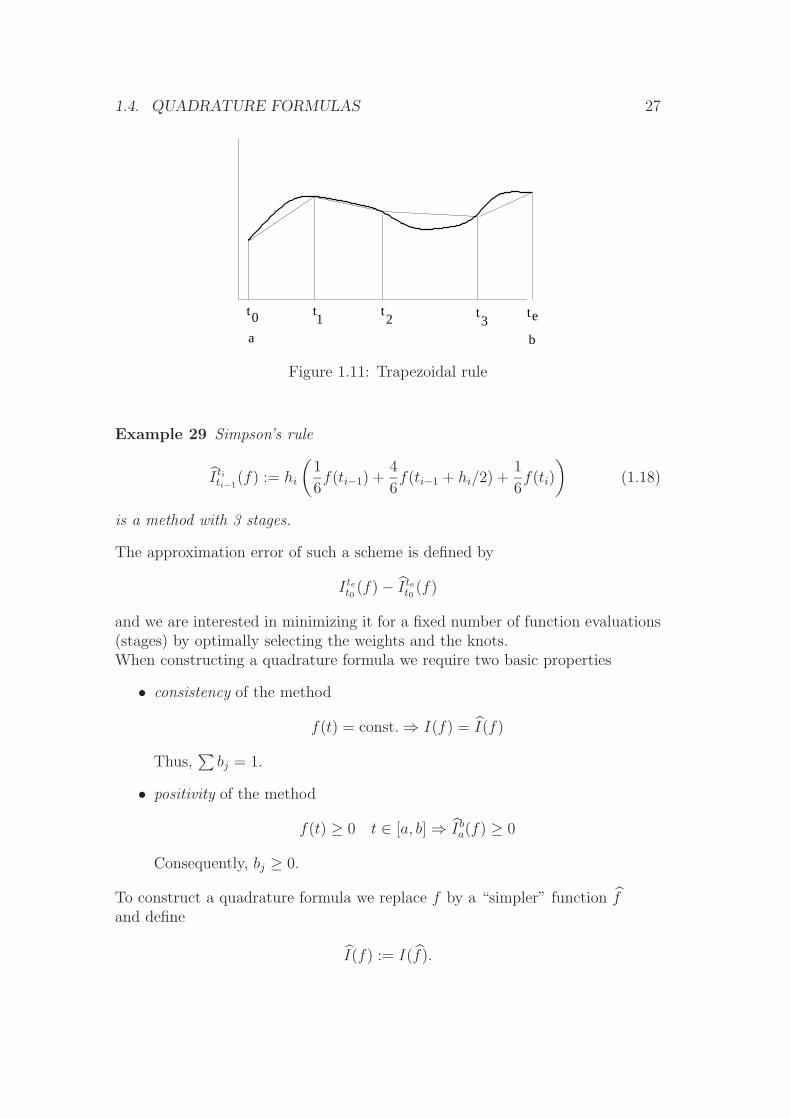
)and hi := ti − ti−1 step size is called trapezoidal rule.
A general scheme for numerical integration can be written as follows
I titi−1(f) := hi
s∑j=1
bjf(ti−1 + cjhi), (1.17)
where s is number of stages, bj are the weights and cj the knots of the quadratureformula.
1.4. QUADRATURE FORMULAS 27
t t t tet0 1 2 3a b
Figure 1.11: Trapezoidal rule
Example 29 Simpson’s rule
I titi−1(f) := hi
(1
6f(ti−1) +
4
6f(ti−1 + hi/2) +
1
6f(ti)
)(1.18)
is a method with 3 stages.
The approximation error of such a scheme is defined by
I tet0 (f)− I tet0 (f)
and we are interested in minimizing it for a fixed number of function evaluations(stages) by optimally selecting the weights and the knots.When constructing a quadrature formula we require two basic properties
• consistency of the method
f(t) = const.⇒ I(f) = I(f)
Thus,∑
bj = 1.
• positivity of the method
f(t) ≥ 0 t ∈ [a, b]⇒ Iba(f) ≥ 0
Consequently, bj ≥ 0.
To construct a quadrature formula we replace f by a “simpler” function fand define
I(f) := I(f).

28 CHAPTER 1. INTERPOLATION AND CURVE DESIGN
Let f be a polynomial interpolating f on the knots τj := ti−1 + cjhi
f(t) := P (f |τ1, . . . , τs)(t) =s∑j=1
f(τj)Ls−1j (t).
Here Ls−1j (t) is the jth Lagrange polynomial defined by the knot points (cf. Sec-
tion 1.2.1)
Ls−1j (t) =
s∏j �=i=1
t− τiτj − τi
.
Thus,
I titi−1(f) =
s∑j=1
f(τj)Ititi−1
(Ls−1j (t)).
Set
bsj :=1
hi
∫ ti
ti−1
Ls−1j (t)dt =
∫ 1
0
Ls−1j (ti−1 + σhi)dσ
then
I titi−1(f) = hi
s∑j=1
bsjf(τj).
Thus, given cj the weights bj are fixed. The methods are consistent due to∑sj=1 L
s−1j (t) = 1. They are exact for polynomials at least up to order s− 1, i.e.
p ∈ Ps−1 ⇒ I(p) = I(p)
Lemma 30Given s distinct points τ1, . . . , τs ∈ [0, 1],then there is a unique functional
I10 (f) =s∑j=1
bjf(τj)
with the propertyI10 (p) = I10 (p) ∀p ∈ Ps−1.
Proof:by construction and the uniqueness of interpolating polynomials. ✷
By coordinate transformation this result applies to any finite time interval anal-ogously.We investigate now the approximation error and define

1.4. QUADRATURE FORMULAS 29
Definition 31If I(p) = I(p) ∀p ∈ Pk−1 and if there is a p0 ∈ Pk with I(p0) �= I(p0), then themethod has order k.
Note, consistent methods have at least order 1.A criterion for the order of a scheme is given by the following theorem:
Theorem 32If∑s
i=1 bicq−1i = 1
qq = 1, . . . , k then the method I has order k.
Proof:Taylor expansion of f about ti. ✷
Example 33It can be easily checked by Taylor expansion that for the trapezoidal rule the localerror is
I titi−1(f)− I titi−1
(f) =1
12f ′′(ti−1)h
3i +O(h4
i )
with hi = ti − ti−1. The global error is bounded by∣∣∣I tet0 (f)− I tet0 (f)∣∣∣ = ∣∣∣∣∣
n∑i=1
I titi−1(f)− I titi−1
(f)
∣∣∣∣∣ ≤ te − t012
maxξ∈[t0,te]
f ′′(ξ)h2 +O(h3)
with h = 1/(te − t0).The power of h in this expression corresponds to the order of the method.
1.4.1 Quadrature in MATLAB
MATLAB provides two commands for computing numerically the integrand of agiven function: quad and quadl . Both methods are adaptive, i.e. the stepsize is MATLABadjusted automatically in such a way, that an error can be guaranteed within auser given tolerance bound. quad is based on Simpson’s rule, while quadl uses amore sophisticated method based on Lobatto polynomials.In this course we will not discuss adaptive quadrature methods. Adaptivity willbe a topic in the chapter concerning ordinary differential equations, see Ch. 5.
1.4.2 Gauss Quadrature
An interesting question in this context is how to place the knots cj so that themethod gets an order k > s. What is the optimal (maximal) order? To an-swer this question some knowledge from the theory of orthogonal polynomialsis required. This will be a topic in one of the advanced courses in NumericalAnalysis, where it can be seen, that the so-called Gauss-methods are optimal.We investigate now the following questions:

30 CHAPTER 1. INTERPOLATION AND CURVE DESIGN
• Can we place the knots cj so that the method gets an order k > s ?
• What is the optimal (maximal) order ?
Theorem 34Define I10 by (ci, bi)
si=1 with order k ≥ s,
and setM(t) := (t− c1)(t− c2) · · · (t− cs) ∈ Ps[0, 1].
The order of I10 is larger than s+m iff∫ 1
0
M(t)p(t)dt = 0 ∀p ∈ Pm−1[0, 1], (1.19)
i.e. M⊥Pm−1[0, 1] in L2.
Proof:Let f ∈ Ps+m−1. Then we can write it as
f(t) = M(t)g(t) + r(t)
with two polynomials g ∈ Pm−1 and r ∈ Ps−1. Consider
I10 (f) = I10 (Mg) + I10 (r).
Due to condition (1.19) the second term vanishes and due to the order of the
method we have I10 (r) = I10 (r).On the other hand
I10 (f) =n∑i=1
bif(ci) =n∑i=1
biM(ci)g(ci) + I10 (r)
where the second term vanishes due to M(ci) = 0. Thus I10 (f) = I10 (f). ✷
Example 35Consider m = 1, s = 3:
0 =
∫ 1
0
(t− c1)(t− c2)(t− c3) · 1dt
=1
4− 1
3(c1 + c2 + c3) +
+1
2(c1c2 + c1c3 + c2c3)− c1c2c3
⇒c3 =
14− (c1 + c2)/3 + c1c2/213− (c1 + c2)/2 + c1c2
Thus, there are two degrees of freedom in designing such a method.

1.4. QUADRATURE FORMULAS 31
Theorem 36A method with s stages has maximal order 2s.
Proof:Assume order k ≥ 2s+ 1. Then by preceding theorem:
0 =
∫ 1
0
M(t)p(t)dt ∀p ∈ Ps[0, 1] (1.20)
especially also for p(t) = M(t). Thus,
0 =
∫ 1
0
M(t)M(t)dt =
∫ 1
0
(t− c1)2 · · · (t− cs)
2dt > 0, (1.21)
which is a contradiction. ✷
Note, the existence of a method of order k = 2s is not stated by this theorem.For constructing such a method we set M(t) = c · Ps(2t − 1), where Ps is theLegendre polynomial of degree s and c a constant such that cPs has the leadingcoefficient 1.Then, by construction ∫ 1
0
M(t)g(t)dt = 0 ∀g ∈ Ps−1. (1.22)
Thus a method based on knots cj with Ps(2cj − 1) = 0 has order k = 2s.
Theorem 37There is a method of order 2s. It is uniquely defined by taking cj as the roots ofthe sth Legendre polynomial Ps(2t− 1).
Example 38
• s = 1 gives the midpoint rule
I10 (f) = f(1
2) (1.23)
• s = 2 Exercise.
• s = 3 gives a 6th order method
I10 (f) =5
18f(
1
2−√15
10) +
8
18f(
1
2) +
5
18f(
1
2+
√15
10). (1.24)
These methods are called Gauß methods.

32 CHAPTER 1. INTERPOLATION AND CURVE DESIGN
1.5 Piecewise Polynomials and Splines
To interpolate a larger amount of data and to avoid effects like Runge’s phe-nomenon as demonstrated in the exercises one applies piecewise polynomial in-terpolation, i.e. constructs a function s which interpolates the data points andwhich is a polynomial between these points.
Definition 39 We consider now functions s ∈ Cr−1[t0, tn] of the following type:
s : [t0, tn]→ R with s[ti,ti+1]
= si ∈ Pr[ti, ti+1] (1.25)
Functions with these properties are called splines (r = 1 linear splines, r = 3cubic splines). We call the points ti knots or breakpoints of the spline s.
The continuity requirements imply
dk
dtksi(ti+1) =
dk
dtksi+1(ti+1) k = 0, . . . , r − 1.
Again, we consider the interpolation task, i.e. we look for a spline function ssatisfying the interpolation conditions:
s(ti) = yi i = 0, . . . , n
A linear spline is easy to construct. It requires to simply draw straight linesbetween the interpolation points.We leave linear and quadratic splines for the exercises and turn directly to cubicsplines, the family of splines, which is most used in applications.For a cubic spline we require that the functions si are cubic polynomials and joinat the knots with C2-continuity. Thus,
si(t) = ai(t− ti)3 + bi(t− ti)
2 + ci(t− ti) + di (1.26)
and we have the following conditions to determine the coefficients ai, bi, ci, di:
si(ti) = yi i = 0, . . . , n− 1 sn−1(tn) = yn (1.27a)
si(ti+1) = si+1(ti+1) i = 0, . . . , n− 2 (1.27b)
s′i(ti+1) = s′i+1(ti+1) i = 0, . . . , n− 2 (1.27c)
s′′i (ti+1) = s′′i+1(ti+1) i = 0, . . . , n− 2 (1.27d)
We have n+1 knots and consequently n intervals and 4n unknowns. To determinethese unknowns we have 4(n− 1)+2 = 4n− 2 conditions. There are two degreesof freedom left. We will fix them later by setting up two additional boundaryconditions.

1.5. PIECEWISE POLYNOMIALS AND SPLINES 33
From (1.27a) we getdi = yi i = 0, . . . , n− 1. (1.28)
We set hi := (ti+1 − ti) and obtain from (1.27b)
yi+1 = aih3i + bih
2i + cihi + yi. (1.29)
The first and second derivatives are
s′i(ti+1) = 3aih2i + 2bihi + ci (1.30a)
s′′i (ti+1) = 6aihi + 2bi (1.30b)
We introduce new variables for the second derivatives at ti, i.e.
Si := s′′i (ti) = 6ai(ti − ti) + 2bi = 2bi (1.31)
From (1.27d) we then obtain
Si+1 = 6aihi + 2bi. (1.32)
Hence,
bi =1
2Si ai =
Si+1 − Si6hi
(1.33)
Inserting these relations into (1.29) gives
yi+1 =(Si+1 − Si
6hi
)h3i +
Si2h2i + cihi + yi.
From that we get ci:
ci =yi+1 − yi
hi− hi
2Si + Si+1
6.
Now we use condition (1.27c) and get
ci = 3ai−1h2i−1 + 2bi−1hi−1 + ci−1.
Inserting the expression for ai, bi and ci gives
yi+1 − yihi
− hi2Si + Si+1
6=
3(Si − Si−1
6hi−1
)h2i−1 + 2
(Si−1
2
)hi−1 +
yi − yi−1
hi−1
− hi−12Si−1 + Si
6
and finally
hi−1Si−1 + 2(hi−1 + hi)Si + hiSi+1 = 6(yi+1 − yi
hi− yi − yi−1
hi−1
)(1.34)

34 CHAPTER 1. INTERPOLATION AND CURVE DESIGN
with i = 1, . . . , n− 1.These are n−1 equations for the n+1 unknown second derivatives Si. We have toask for two more conditions, which are boundary conditions if we put conditionson S0 and Sn.The easiest is to ask for
S0 = Sn = 0. (1.35)
A cubic spline fulfilling this condition is called a natural spline. We will firstconsider this possibility and then discuss other common choices of boundaryconditions.Equations (1.34) and (1.35) give us a square linear system of equations which canbe solved to determine the Si:
2(h0 + h1) h1
h1 2(h1 + h2) h2
h2. . . h3
. . . hn−2
hn−2 2(hn−2 + hn−1)
S1
S2
S3...
Sn−1
=
= 6
y2−y1h1− y1−y0
h0y3−y2h2− y2−y1
h1......
yn−yn−1
hn−1− yn−1−yn−2
hn−2
(1.36)
Note, the ”empty” entries in the coefficient matrix are zeros. The matrix has abanded structure. It is a tridiagonal matrix , furthermore it is symmetric. Howthis structure can be exploited when solving the system will be discussed inChapter 2. Here we just use the corresponding MATLAB commandMATLAB
S=A\b
for solving the system. For defining the coefficient matrix we can use the factthat the matrix is banded and apply MATLAB’s command ”diag”, cf. ”helpMATLABdiag” and the exercises.As pointed out before the definition of a cubic spline leaves two degrees of freedom.These are normally described in terms of boundary conditions. There are severalcommon choices
• natural spline: We take S0 = Sn = 0. This choice is often taken, if we haveno other specific information available.
• end slope condition We might have knowledge about the slopes at theboundary points, i.e. s′(t0) and s′(tn) are known. From that conditionsfor S0 and S1 can be derived and the linear system corresponding to (1.36)can be set up. We leave this as an exercise.
1.5. PIECEWISE POLYNOMIALS AND SPLINES 35
• periodic spline: We assume, that the function we want to interpolate is aperiodic function with a period tn− t0. From that we can conclude s′(t0) =s′(tn) and S0 = s′′(t0) = s′′(tn) = Sn. Which gives enough conditions touniquely define the spline.
• not-a-knot condition: If the physical context gives no additional informationabout the spline at the boundary, one may fix the boundary conditions bythe additional requirements
s′′′0 (t1) = s′′′1 (t2) s′′′n−2(tn−1) = s′′′n−1(tn−1). (1.37)
By this s0 and s1 become a cubic parabola and the point t1 is no longer aknot. The same holds for sn−2, sn−1 and tn−1. This motivates the nameof this type of boundary conditions. The MATLAB function ”spline” usesthis type of boundary condition. MATLAB
In MATLAB’s spline toolbox there are many additional tools for computing and MATLABevaluating splines. A command that computes spline coefficient for various endconditions is csape.
1.5.1 Minimal Property of Cubic Splines
The Webster gives the following historical description of the word spline ”a thinwood or metal strip used in building construction” (1756). When bending astraight piece of metal along some nails (interpolation points) its deformation isdefined by minimizing the deformation energy. Let the curve be a function s withthe property s(ti) = yi, where (ti, yi) are the coordinates of the nails, then thiscurve has the property ∫ te
t0
(s′′)2(t)dt = min ‖f ′′‖22
(up to physical constants, like the elasticity coefficient), where the minimum istaken over all C2 functions satisfying the interpolation conditions.
In this subsection we will show, that the cubic spline functions indeed share thisproperty.
We denote by V the set of all C2 functions which interpolate the points (ti, yi)with i = 0, . . . , l + 1.
Theorem 40Let s∗ ∈ V be a cubic spline satisfying a natural boundary condition. Then‖s∗′′‖2 ≤ ‖s′′‖2 ∀s ∈ V.
36 CHAPTER 1. INTERPOLATION AND CURVE DESIGN
Proof:Let s ∈ V, then there is a h ∈ C2 with h(ti) = 0 such that s(t) = s∗(t)+ h(t). Wethen obtain
‖s′′‖22 = ‖s∗′′ + h‖22 = ‖s∗′′‖2 + 2 < s∗′′, h′′ > +‖h′′‖22with
< s∗′′, h′′ >:=
∫ te
t0
s∗′′(t)h′′(t)dt.
We have to show that < s∗′′, h′′ >= 0:Integration by parts gives
< s∗′′, h′′ >= s∗′′(t)h′(t) tet0−∫ te
t0
s∗′′′(t)h′(t)dt.
From the natural boundary conditions follows
s∗′′(t)h′(t) |tet0 = 0.
As s∗ is a piecewise cubic polynomial we get for the last term∫ te
t0
s∗′′′(t)h′(t) =∑
αi
∫ ti
ti−1
h′(t) =∑
αi(h(ti)− h(ti−1)) = 0
with some constants αi. ✷
1.5.2 B-Splines
In this subsection we study the linear space of splines like we did before forpolynomial spaces and look for a basis of this space which gives us spline repre-sentations with ”nice” coefficients. By ”nice” we mean in the context of graphics,coefficients which have a direct geometrical interpretation. By changing the coef-ficients we want to influence the shape of the spline only locally. We saw this taskalready when discussing the Bernstein basis for polynomials. For the interpola-tion task it plays the interpretation of the coefficients plays not a certain role, butwhen using splines for design purposes the coefficients can solve as ”handles” toinfluence the shape by positioning them through mouse clicks or other computerinput devices.Let ∆ := {a = t0, t1, . . . , tl+1 = b} with ti < ti+1 denote a partitioning (or a grid)of the interval [a, b].The space of all splines of degree k − 1 with respect to ∆ is denoted by Sk,∆. Itis easily checked that Sk,∆ is a linear space and evidently Pk−1 ⊂ Sk,∆ holds.

1.5. PIECEWISE POLYNOMIALS AND SPLINES 37
Thus a basis of Sk,∆ consists of a basis of the polynomial space plus some addi-tional functions. Let us consider first the monomial basis of the polynomial spaceand extend it to a basis of the spline space.For this end we define
Definition 41
(t− ti)k−1+ :=
{(t− ti)
k−1 if t ≥ ti0 else.
Theorem 42B := {1, t, . . . , tk−1, (t− t1)
k−1+ , . . . , (t− tl)
k−1+ } is a basis of Sk,∆ and dimSk,∆ =
k + l.
Note, the numbering. Why are the functions (t− t0)k−1+ and (t− tl+1)
k−1+ corre-
sponding to the first and the last grid point not taken as basis functions?
Example 43 If we consider cubic splines (k = 4) and l = n − 1 we obtaindimSk,∆ = 4 + n − 1 = 2 + n + 1. So, when uniquely defining a spline we haveto give as many conditions for the coefficients. In the interpolation task we fixedthem by n+ 1 interpolation conditions plus two boundary conditions.
With this theorem we got an easy way to determine the dimension of a spline spacebut for computational purposes there are better ways to choose basis functions,which lead us to B-splines.We formally extend the grid to
∆ : τ1 = . . . = τk < τk+1 < . . . < τk+l+1 = . . . = τk+l+k
with τk+i = ti for i = 0, . . . , l and define
Definition 44The functions Nik defined recursively as follows are called B-splines:
Ni1(t) :=
0 if τi = τi+1
1 if t ∈ [τi, τi+1)0 else
and
Nik :=t− τi
τi+k−1 − τiNi,k−1 +
τi+k − t
τi+k − τi+1
Ni+1,k−1
where we use the convention 0/0 = 0 if nodes coincide.
Examples of these functions are depicted in Fig. 1.12. There one observes the in-creasing degree of smoothness when raising the order of these functions. Withoutproof we collect some important properties of these functions:
1. Nik(t) �= 0 only for t ∈ [τi, τi+k]: local support

38 CHAPTER 1. INTERPOLATION AND CURVE DESIGN
0
0.2
0.4
0.6
0.8
1
1.2
τi
τi+1
τi+2
τi+3
τi+4
Ni1
Ni2
Ni3
Ni4
Figure 1.12: B-splines of order up to 4
2. Nik(t) ≥ 0: non-negative
3. Nik ∈ Sk,∆ if τi �= τi+k: B-splines are splines
4. Nik ∈ Ck−1−m if there are m-fold knots τj.
The last property may be used for modeling corners, see Fig. 1.13.
1 1.5 2 2.5 3 3.5 4−0.2
0
0.2
0.4
0.6
0.8
1
1.2
Figure 1.13: N13 generated with a double knot at τ = 3
Theorem 45 The B-splines Nik, i = 1, . . . l + k form a basis of Sk,∆.Therefore has any function s ∈ Sk,∆ a unique representation
s =l+k∑i=1
diNik

1.5. PIECEWISE POLYNOMIALS AND SPLINES 39
and in particular
1 =l+k∑i=1
Nik.
The coefficients di are called de Boor points. See also their role in the context ofBezier splines.Changing the di’s influences only a local part of the total spline due to the localsupport property of the B-splines. The degree of the B-spline determines thenumber of intervals influenced by this change.More on this subject can be found in [de 78, Far88].

40 CHAPTER 1. INTERPOLATION AND CURVE DESIGN

Chapter 2
Linear Systems
We saw in the preceding sections the need for solving linear systems. They oc-curred when we wanted to solve the Vandermonde or Bezier system for polynomialinterpolation and in a special form (tridiagonal system) when computing cubicinterpolation splines.Solving linear systems occurs in nearly all algorithms in numerical analysis as asubproblem. It has the following form
Ax = b with A ∈ Rn×m
In this course we study the following cases
• n = m square systems
• n > m overdetermined systems
As n and m can be very large (up to 104 unknowns) computing time for solvingthese systems can become crucial.So long in this course we just solved these systems by using the MATLAB com- MATLABmand1.
x = A \ b
Now, we go into details and look what this command actually does.We first review some facts on solvability of linear systems.
Definition 46The linear space
N (A) = {x ∈ Rm|Ax = 0}
is called the nullspace or kernel of A and
R(A) = {z ∈ Rn|∃x ∈ R
mAx = z}is called the range space or image space of A.
1For MATLAB help on the ”\” command, type help mldivide
41
42 CHAPTER 2. LINEAR SYSTEMS
(see also [Spa94, p. 143,144]).We note,
det(A) �= 0 ≡ N (A) = {0} .If det(A) �= 0 the matrix is called non singular. If n = m a non singular matrixis also called regular.
Theorem 47 The linear system Ax = b has a solution, if b ∈ R(A).The solution is unique, if N (A) = {0}.We will first consider the case n = m and only regular matrices.
2.1 Regular Linear Systems
2.1.1 LU Decomposition
Definition 48 A matrix L is called a lower triangular matrix if all elementsover its diagonal are zero. Furthermore, if its diagonal elements are one, then itis called unit lower triangular.
Here an example for a unit lower triangular matrix.
L =
1 0 0 0 0 0l21 1 0 0 0 0l31 l32 1 0 0 0l41 l42 l43 1 0 0l51 l52 l53 l54 1 0l61 l62 l63 l64 l65 1
.
An example for a lower triangular matrix is given in Eq.(1.7).Correspondingly we speak of an upper triangular matrix U if its entries underthe diagonal are zero. Here an example:
U =
u11 u12 u13 u14 u15 u16
0 u22 u23 u24 u25 u26
0 0 u33 u34 u35 u36
0 0 0 u44 u45 u46
0 0 0 0 u55 u56
0 0 0 0 0 u66
.
We assume, that we can factorize A into a product of a lower and upper triangularmatrix: A = LU . Then the linear system can be written as
Ax = b (2.1a)
LUx = b (2.1b)
Ly = b (2.1c)

2.1. REGULAR LINEAR SYSTEMS 43
withy := Ux (2.1d)
This suggests the following algorithm
• LU Factorization: Decompose A into a product of a lower triangular matrixL and an upper triangular matrix U .
• Forward substitution Solve Ly = b for y by exploiting the triangular struc-ture of L.
• Backward substitution Solve Ux = y for x by exploiting the triangularstructure of U .
Before considering a method for performing the decomposition step, we look atthe two substitution steps.
Forward and backward substitutionConsider the example of a lower triangular system of the type Ly = b:
b1 = l11y1
b2 = l21y1 + l22y2...
b5 = l51y1 + l52y2 + l53y3 + l54y4 + l55y5
From the first equation you immediately get y1. Using this value, you easilyobtain y2 from the next equation and so on.We describe the procedure for a general lower triangular matrix by the followingpiece of MATLAB code: MATLAB
for i=1:n;
for j=1:i-1;
b(i)=b(i)-l(i,j)*b(j);
end;
b(i)=b(i)/l(i,i);
end;
y=b;
Here a similar example of an upper triangular system Ux = y:
y1 = u11x1 + u12x2 + u13x3 + u14x4 + u15x5
y2 = u22x2 + u23x3 + u24x4 + u25x5
...
y5 = u55x5

44 CHAPTER 2. LINEAR SYSTEMS
For solving this system, we start with the last equation and solve for y5 andproceed in a similar way but backwards.In MATLAB code this readsMATLAB
for i=n:-1:1;
for j=i+1:n
y(i)=y(i)-u(i,j)*y(j);
end;
y(i)=y(i)/u(i,i);
end;
x=y;
Counting operations gives n2/2+O(n) multiplications and as many additions forthe backward or forward substitution methods2
Elementary transformations We turn now to the decomposition step andshow the principal idea by transforming A stepwise into an upper triangular ma-trix by multiplication with so-called elementary transformation matrices. Again,we explain things first by looking at an example of a 5× 5 matrix:
1−l21 1...
. . .
−ln1 1
︸ ︷︷ ︸
=:M1
a11 a12 . . . a1na21 a22...
. . .
an1 ann
︸ ︷︷ ︸
=:A
=
a11 a12 . . . a1n0 a
(1)22 a
(1)2n
.... . .
0 a(1)n2 . . . a
(1)nn
︸ ︷︷ ︸
=:A(1)
witha(1)ij := aij − li1 a1j j = i, . . . , n
and li1 := ai1/a11.We observe, that premultiplying A by M1 annihilates all but the first element inthe first column of A and changes all other elements but those in the first row.In general an elementary transformation matrix has the following form:
Mk :=
1. . .
1
−lk+1,k. . .
...−ln,k 1
(2.2)
2Operations are counted often in a ”unit” called flop, which stands for floating point oper-ation and corresponds to an addition or multiplication. See the MATLAB command flops.

2.1. REGULAR LINEAR SYSTEMS 45
with lik := a(k−1)ik /a
(k−1)kk and A(k−1) := Mk−1 · · ·M1A and A(0) := A.
Elementary transformations are regular matrices and their inverses have a similarstructure:
M−1k :=
1. . .
1
lk+1,k. . .
...ln,k 1
(2.3)
We note two important facts in this context (which can be checked easily):
• Products of triangular matrices are triangular.
• Inverses of upper (lower) triangular matrices are upper (lower) triangular(if they exist).
We setU := Mn−1Mn−2 . . .M2M1︸ ︷︷ ︸
L−1
A
with an upper triangular matrix U and a lower triangular L.Thus we got the LU -factorization of A
A = LU (2.4)
with L = M−11 . . .M−1
n−2M−1n−1.
We call a(k−1)kk the pivot element at stage k. The matrix A has an LU factorization
as long as all pivot elements are different from zero.The derivation above is not a description of an algorithm. Setting up all ele-mentary transformations explicitly and performing multiplications with matriceswhich have very few non zero entries would be an enormous waste of computingresources.We give an algorithm for the LU factorization as a short segment of a piece ofMATLAB code: MATLAB
function [L,U]=lu_np(A)
% Factorizes A into a lower and an
% upper triangular part without pivoting.
% This code does not correspond to MATLAB’s command lu .
N=size(A,1);
if N~=size(A,2)
disp(’Matrix has to be square’)
break
46 CHAPTER 2. LINEAR SYSTEMS
end
for i=1:N,
pivot=A(i,i);
if pivot==0
disp(’Matrix has zero pivot elements’)
break
end
for j=i:N,
L(j,i)=A(j,i)/pivot;
end
for k=i+1:N,
for j=i+1:N,
A(k,j)=A(k,j)-L(k,i)*A(i,j);
end
end
end
U=zeros(N,N);
for i=1:N,for j=i:N, U(i,j)=A(i,j);end;end;
Note every regular matrix can be LU factorized. The pivot elements might bezero which will lead to a break in the algorithm. This can be seen from thefollowing (regular) example: (
0 11 0
)(x1
x2
)=
(b1b2
)We will give a criterion for matrices which are LU factorizable.
Definition 49A is called diagonal row dominant iff
|aii| >n∑j �=i|aij| ∀i = 1, . . . , n
Theorem 50Every diagonal dominant matrix A has an LU decomposition.
If A is diagonal dominant, then also all A(k), and
maxij|a(k+1)ij | ≤ max
ij|a(k)ij | ≤ max
ij|aij|.
From the example above we see, that a matrix which has no LU factorizationcan be transformed into a matrix which has an LU factorization by permutingthe rows: (
1 00 1
)(x1
x2
)=
(b2b1
)
2.1. REGULAR LINEAR SYSTEMS 47
Interchanging rows of a matrix can mathematically expressed by premultiplica-tion by a permutation matrix P . Permutations are row permuted identity ma-trices. Here an example of a matrix which permutes the second with the fourthrow when premultiplying a 4× 4 matrix.
1 0 0 00 0 0 10 0 1 00 1 0 0
We modify now the LU factorization above by introducing row permutationsafter each step: In general the rows have to be interchanged
A(k+1) = MkPkA(k)
with permutation matrix Pk which interchanges the rows in such a way thatthe pivot element becomes the largest element in the column segment a(:, k : n)(MATLAB notation). Consequently, MATLAB
|lik| ≤ 1 i = k + 1, . . . , n.
Looking for the largest element in a column and then interchanging rows is calledpartial pivoting in contrast complete pivoting which is a more seldom appliedstrategy. There one attempts to interchange both rows and columns to obtaina pivot element which is the largest element in the actual submatrix in the k-thstep.
Theorem 51 If A is a regular matrix, there is always a permutation matrix P ,such that PA has an LU factorization.
In MATLAB LU-factorization with pivoting is performed by the command lu. MATLABIt returns the triangular factors and the permutation matrix.We conclude this section by counting the operations which are required for LUfactorization. It can be read from the MATLAB code LU np above, that
N−1∑i=1
(N − i)2 =N−1∑k=1
k2 =( N∑k=1
k2)−N2
multiplications and as many additions are needed.By noting,
k2 =
∫ k
k−1
x2dx+ k − 1
3
andN∑k=1
k2 =N∑k=1
(
∫ k
k−1
x2dx+ k − 1
3)

48 CHAPTER 2. LINEAR SYSTEMS
we finally get ( N∑k=1
k2)−N2 =
N3
3− N2
2+
N
6
multiplications for LU decomposition. Additionally we have to perform N(N −1)/2 divisions.Often we have to solve the same linear system for different right hand sides b.In that case the factorization step needs only to be performed once and only the(cheaper) forward and backward substitution steps have to be performed for thedifferent right hand sides. A particular example is the numerical evaluation ofthe mathematical expression
A−1B
This can be rewritten as aAX = B
where X is a matrix with columns x(i). Every column is then the solution of alinear system
Ax(i) = b(i).
2.1.2 Matrix Norms, Inner Products and Condition Num-bers
Numerical computations are always influenced by errors. The errors in the resultsof our algorithms we considered so far have mainly two sources
• Round-off errors
• errors in the input data .
Later we will meet a third error source, the truncation error when solving thingsiteratively.In order to study the effects of errors we have to be able to measure the size oferrors. Errors are often described as relative quantities, i.e.
relative error =absolute error
exact solution
and as the exact solution often is not available we consider instead
relative error =absolute error
obtained solution.
An error in the result of a linear system is a vector, thus we have to be able tomeasure sizes of vectors.For this end we introduce norms

2.1. REGULAR LINEAR SYSTEMS 49
Definition 52A vector norm is defined by ‖.‖ : R
n → R with
• ‖x‖ ≥ 0
• ‖x‖ = 0⇔ x = 0
• ‖x+ y‖ ≤ ‖x‖+ ‖y‖• ‖αx‖ = |α|‖x‖ α ∈ R
(see also [Spa94, p. 111]).Norms we use in this course:
‖x‖p := (|x1|p + . . .+ |xn|p)1/p
so-called p-norm or Holder-norm.
Example 53‖x‖1 = |x1|+ . . .+ |xn|‖x‖2 = (|x1|2 + . . .+ |xn|2)1/2 (Euklid)‖x‖∞ = max |xi|Theorem 54All norms on R
n are equivalent in the sense:There are constants c1, c2 > 0 such that for all x
c1‖x‖α ≤ ‖x‖β ≤ c2‖x‖αholds.
Example 55
‖x‖∞ ≤ ‖x‖2 ≤√n‖x‖∞
‖x‖2 ≤ ‖x‖1 ≤√n‖x‖2
‖x‖∞ ≤ ‖x‖1 ≤ n‖x‖∞Recall from your calculus course, that the definition of convergence is based onnorms. The ultimate consequence of this theorem is that an iteration processin a finite dimensional space converging in one norm is also converging in anyother norm. For proving convergence we just can select a norm which is the mostconvenient for the particular proof. Note, that in infinite dimensional spaces(function spaces) this nice property is lost.We relate now vector norms to matrices. The concept is highly based on viewingmatrices as linear maps
A : Rn −→ R
n.

50 CHAPTER 2. LINEAR SYSTEMS
Definition 56
‖A‖p = maxx �=0
‖Ax‖p‖x‖p = max
‖x‖p=1‖Ax‖p
defines a matrix norm, which is called subordinate to the vector norm ‖x‖p.Some matrix norms:
‖A‖1 = max j∑
i ‖aij‖
‖A‖2 =√
maxi λi(ATA) where λi(A) denotes the i-th eigenvalue of A
‖A‖∞ = maxi∑
j ‖aij‖
‖A‖F =(∑
i
∑j |aij|2
)1/2(Frobenius Norm)
Vector and matrix norms can be computed in MATLAB by the command norm,MATLABwhich takes additional argument to define the type of norm, i.e. ’inf’ standsfor infinity norm.We consider now the sensitivity of the linear system Ax = b with respect toperturbations ∆b of the input data b.
Ax = A(x+∆x) = b+∆b (2.5)
How is the relative input error‖∆b‖‖b‖
related to the relative output error
‖∆x‖‖x‖ ?
FromA∆x = ∆b⇒ ∆x = A−1∆b
we obtain by taking norms
∆x = A−1∆b⇒ ‖∆x‖ ≤ ‖A−1‖‖∆b‖.
2.1. REGULAR LINEAR SYSTEMS 51
Note that the right inequality is a direct consequence from Def. 56. Analogouslywe get
b = Ax⇒ ‖b‖ ≤ ‖A‖‖x‖.This leads to,
‖∆x‖‖x‖ ≤
‖A−1‖ ‖∆b‖‖x‖ =
‖A‖ ‖A−1‖‖∆b‖‖A‖‖x‖
Thus,‖∆x‖‖x‖ ≤ ‖A‖ ‖A
−1‖‖∆b‖‖b‖
Definition 57 κ(A) := ‖A‖‖A−1‖ is called the condition number of A.
Condition numbers can obtained in MATLAB by using the commands cond and MATLABrcond. The first command computes the condition number exactly and takes asargument a specification of the type of norm used for computing this number.rcond estimates the inverse of the condition number κ(A)−1 with respect to the1-norm.We consider also perturbations of the matrix A:
(A+∆A)(x+∆x) = b
and define for this end: A(t) := A+ t∆A and x(t) := x+ t∆x, with t ∈ R.Consider:
A(t)x(t) = b
and take the derivative w.r.t. t:
A′(t)x(t) + A(t)x′(t) = 0
x′(t) = −A(t)−1A′(t)x(t)
Thus,
‖x′‖‖x‖ ≤ ‖A
−1‖ ‖A′‖
≤ ‖A−1‖ ‖A‖‖A′‖
‖A‖Note, A′(t) = ∆A and x′(t) = ∆x. Thus
‖∆x‖‖x‖ ≤ κ(A)
‖∆A‖‖A‖
Example 58 The relative error due to round-off is called the so-called machineepsilon. Usually we have ε ≈ 10−16 when using double precision arithmetic.

52 CHAPTER 2. LINEAR SYSTEMS
If there is no other error in the input data we obtain
‖∆x‖‖x‖ ≤ κ(A)ε
If κ(A) = 1 no amplification of the relative input error occurs. If κ(A) = 10k weloose in the worst case k digits of accuracy.
The number κ(A)−1 can be viewed as the distance from A to the nearest singularmatrix.
2.2 Nonsquare Linear Systems
In this section, we consider linear systems of the form
Ax = b with A ∈ Rm×n
with m" n. This kind of problem often occurs when performing data fitting.
Example 59We would like to fit the data
i 0 1 2 3 4ti -1.0 -0.5 0.0 0.5 1.0yi 1.0 0.5 0.0 0.5 2.0
by a quadratic polynomial of the form
p(t) = a2t2 + a1t+ a0.
We set up interpolation conditions p(ti) = yi:1 t0 t201 t1 t211 t2 t221 t3 t231 t4 t24
a0
a1a2
=
y0y1y2y3y4
.
This leads to a nonsquare linear system. It is overdetermined in the sense, thatalready three data points would have been enough to uniquely define a quadraticpolynomial.In general, this linear systems has no solution at all, because the measurementsmight not fit to a quadratic polynomial.While often physical laws determine the degree of the polynomial this effect isdue to measurement errors. Just reducing the amount of information to make

2.2. NONSQUARE LINEAR SYSTEMS 53
the system solvable would be the wrong way to attack the problem, because asingle erroneous measurement gets a too strong influence on the result.Therefore we formulate the problem in a different way:Find an x with
‖Ax− b‖2 = minx‖Ax− b‖2 = min
x‖r(x)‖2 (2.6)
with the residual vectors r(x) := b− Ax.A necessary condition for x to be a minimizer is
d
dx‖r(x)‖22 x=x
= 0. (2.7)
From
‖r(x)‖22 = rTr = (b− Ax)T(b− Ax) = bTb− 2xTATb+ xTATAx
we take the first derivative w.r.t. x.This gives the condition for x :
ATAx− ATb = 0 (2.8)
These equations are called normal equations and their solution a least squaressolution of the overdetermined linear system.Normal equations have a geometric interpretation: Consider the range spaceR(A). It is spanned by the columns of A.By writing the normal equations as
AT(b− Ax) = ATr(x) = 0
we see that the residual corresponding to the least squares solution has to benormal (orthogonal) to the columns of A or, in other words, to the range spaceof A. This justifies the name ”normal” equations. This result can be generalizedas follows
Theorem 60Let V be a finite dimensional linear space with an inner product < ·, · >. LetU ⊂ V be a subspace and
U⊥ := {v ∈ V | < v, u >= 0 ∀u ∈ U}be its orthogonal complement in V .Then, for all v ∈ V
‖v − u∗‖ = minu∈U‖v − u‖ ⇔ v − u ∈ U⊥ (2.9)
with the norm ‖v‖ = (< v, v >)1/2 induced by the inner product < ·, · >.

54 CHAPTER 2. LINEAR SYSTEMS
rb
A x
Im(A)
Figure 2.1: Geometric interpretation of the normal equations
Proof:Let u∗ ∈ U be the unique point with v − u∗ ∈ U⊥. (Why is this point unique?)Then for all u ∈ U we have
‖v − u‖2 = ‖v − u∗‖+ 2 < v − u∗, u∗ − u > +‖u∗ − u‖2= ‖v − u∗‖2 + ‖u∗ − u‖2 ≥ ‖v − u∗‖2
where equality holds only for u = u∗. ✷
To compute the least squares solution from the normal equations requires to firstform the matrix ATA. It can be shown that the condition number is squared bythis process, which will result in an unnecessary high sensitivity with respect toperturbations. This can be avoided by using special techniques like orthogonalfactorization of A or singular value decomposition [Hea97].Overdetermined systems are solved in MATLAB with the same command asMATLABsquare systems, i.e. by using ”\”. Note, that totally different algorithms areperformed by one and the same command. In the overdetermined case caseMATLAB does not solve the least squares problem by directly setting up andsolving the normal equations. MATLAB uses for stability reasons, which will beexplained later, orthogonal factorizations (see Sec. 2.2.3) instead.
2.2.1 Projections
From Fig.2.1 it is intuitively clear that the normal equations and the least squaresapproach are related to projections. In linear algebra projections are defined by
Definition 61An n× n matrix P is called an orthogonal projection if it satisfies

2.2. NONSQUARE LINEAR SYSTEMS 55
• P 2 = P
• PT = P
As Pv ∈ Range(P ) we also say that P projects onto Range(P ).Orthogonal projections have the property that the vector v − Pv is orthogonalto any vector in Range(P ):
< v − Pv, Px >= vTPx− vTPTPx = vTPx− vP 2x = 0
Example 62
• The solution of the normal equations is the projection of b onto RangeAbecause A(ATA)−1AT is a projector on Range(A).
• If P is an orthogonal projector so is I − P an orthogonal projector onRange(P )⊥.
• ‖w‖2 = 1 P = I − wwT is a projector on the hyperplane wTx = 0.
• Q1 = (q1, . . . , qr) an m× r matrix,with QT
1 Q1 = I, thenQ1Q
T1 projector on R(Q1)
I −Q1QT1 projector on R(Q1)
⊥ = N(Q1)
• A projector is singular or the identity.
2.2.2 Condition of Least Squares Problems
We investigate now the sensitivity of least squares solutions with respect to per-turbations of the right hand side b (measurements) and with respect to pertur-bations of the matrix A (time points).For this end we first define
Definition 63The angle δ between b ∈ X and a subspace U ⊂ X is defined by
sin δ =‖b− Pb‖2‖b‖2 ,
where P is an orthogonal projection onto U (see Fig. 2.1).
The following theorem relates this angle to the condition of the least squaresproblem with respect to perturbations of the data (perturbations in measurements= perturbations of b, perturbations in measurement time = perturbation in A):

56 CHAPTER 2. LINEAR SYSTEMS
Theorem 64 (Condition of a least squares problem)Let A ∈ R
m×n be a full rank matrix, b ∈ Rn and consider the least squares problem
min ‖Ax− b‖2.The condition number of this problem
• with respect to perturbations in b is given by
κ ≤ κ2(A)
cos δ
• and with respect to perturbations in A
κ ≤ κ2(A) + κ2(A)2 tan δ
Here κ2(A) :=(maxi λi(A
TA)mini λi(ATA)
)1/2is the condition number of A with respect to ‖ · ‖2
and δ is the angle between b and R(A) as defined above.
In the extreme case that δ = π/2 the condition becomes infinity, which expressesthe fact that the data has no relation to the problem. This indicates a wrongmodel of the physical problem.On the other hand, if δ is small, than the condition number is of the size of κ(A).It is worth while to compare this fact to the condition of the normal equationswhich is
κ2(ATA) = κ2(A)2.
Thus, often the condition of least squares problem is significantly smaller thanthe condition of the normal equations and one would introduce an ”artificial”sensitivity with respect to perturbations if one would attempt to solve the leastsquares problem via the normal equation. So we seek for an alternative charac-terization of the least squares solution, which avoids forming the matrix ATA.This alternative way may be computationally more expensive but it will be morestable, i.e. less sensitive to perturbations.For this end we will discuss orthogonal factorizations of A in the next subsection.
2.2.3 Orthogonal factorizations
First, we recall the definition of an orthogonal matrix:
Definition 65 An n× n matrix Q is called orthogonal if
QTQ = I

2.2. NONSQUARE LINEAR SYSTEMS 57
First, note that a orthogonal projection is only in the trivial case P = I describedby an orthogonal matrix. So do not confound the terms.A direct consequence of the definition is det(Q) = ±1 (see determinant multi-plication theorem). Furthermore we see from the definition of the 2-norm ‖ · ‖that for orthogonal matrices ‖Q‖2 = 1 holds. This makes orthogonal matrices soimportant in numerical analysis: Transformations by orthogonal matrices do notchange the condition of linear systems.
Example 66
• Rotations (det(Q) = +1) are described by orthogonal matrices. A 2 × 2rotation matrix is given by
Q =
(cos θ sin θ− sin θ cos θ
)• Reflections (det(Q) = −1) are described by orthogonal matrices. A 2 × 2reflection matrix has the form
Q =
(cos θ sin θsin θ − cos θ
)We assume now that we can write the m×n matrix A as a product of an m×morthogonal matrix Q and an m× n upper triangular matrix R:
A = QR
or schematically: We can reformulate the normal equations Eq. 2.8 by using this
=0
R
RQA =
Q1Q2
A1
factorizations:
ATAx− ATb = RTQTQRx−RTQTb
RT1 R1x = RT
1 QT1 b
R1x = QT1 b.
So, instead of solving the normal equations we can solve
R1x = QT1 b (2.10)

58 CHAPTER 2. LINEAR SYSTEMS
and we avoid forming the product ATA.By the relation
‖Ax− b‖22 = ‖QT(Ax− b)‖22 = ‖R1x−QT1 b‖22 + ‖QT
2 b‖22we obtain even an expression for the norm of the residual of the least squaressolution:
‖r‖2 := min ‖Ax− b‖2 = ‖QT2 b‖2
In MATLAB there is a command qr performing QR-factorization. The numericalMATLABalgorithm is based on either successive rotations of the coordinate system orsuccessive reflections corresponding to the geometric interpretation of orthogonalmatrices given above.
2.2.4 Householder Reflections and Givens Rotations
• Householder reflections
• Givens rotations.
In this course we will discuss only Householder reflections and refer to literature,e.g. [Gv96], for Givens rotations.The principal idea of of Householder reflections can be described geometrically:Given a vector v, a reflection across span(v)⊥ is given by the (orthogonal) matrix
H = I − 2vvT
vTv
(Check that Hx = x for all x ∈ span(v)⊥.)
v a
Haspan(v)
Figure 2.2: Reflection across span(v)⊥
We select a vector v in such a way that it reflects a given vector a such that
Ha = H
a1a2...
am
=
a10...0
.

2.2. NONSQUARE LINEAR SYSTEMS 59
This can be achieved by setting v = a ∓ σe1 σ := ‖a‖2.. It can easily checkedthat with this choice Ha = σe1.This special choice of v is illustrated in Fig. 2.3. The method is best illustrated
v a
Ha
Figure 2.3: Householder tranformation for annihilating entries in a vector
by the following MATLAB sequence MATLAB
function [v]=house(a1,m)
% [v]=function house(a1,m)
% computes a householdermatrix to
% transform the m-vector a1 into
% sigma e_1, where e_1 is the
% first unit vector and sigma is
% up to a sign norm(a1)
%
sigma=norm(a1);
e1=zeros(m,1);
e1(1)=1;
alpha=a1’*e1;
v=a1+sign(alpha)*sigma*e1;
gamma=sigma*(sigma+abs(alpha));
sigma=-sign(alpha)*sigma;
This code applied to the vector a :=(1 2 3
)Tgives the following result Ha :=(−3.7417 0 0
)T.
It is important to note that multiplications with Householder matrices can bedone with n+ 1 multiplications and additions as
Ha = (I − vvT
γ)a = a− 1
γ(vTa)v
with γ := 1/2 vTv. (Standard matrix vector multiplications requires n2 multipli-cations and additions.
60 CHAPTER 2. LINEAR SYSTEMS
With this elementary Householder transformations a matrix can be transformedinto a triangular matrix. We apply for this end n−1 Householder transformationsH1, ..., Hn−1 to A, where the ith transformation introduces zeros in the ith column,while leaving the columns 1, . . . , i− 1 unaffected.To demonstrate the process we assume that the first two columns are alreadytransformed, i.e
H2H1A =
x x x x x0 x x x x0 0 a33 x x0 0 ? x x0 0 ? x x
.
The goal for the third transformation is then to construct a Householder matrixH3 with
H3
a33??
=
a3300
.
Then we set
H3 =
(I 0
0 H3
)where we augment H3 by the identity matrix to keep the earlier columns of Aunaffected.If we set then QT = Hn−1 · . . . ·H1 we obtain QTA = R, where R is the desiredtriangular matrix and we thus got the descomposition A = QR. For implemen-tational details see [Gv96].
2.2.5 Rank Deficient Least Squares Problems
So far we assumed A ∈ Rm×n to be a full-rank matrix (Rank(A) = max(n,m)).
Now we consider the general case:Rank(A) ≤ max(n,m).The least squares problem (and the normal equations) still has a solution but itis no longer unique.We are interested to compute among those solutions, the solution with the leastEuclidean norm. Thus we have to solve the problem:
minx∈L(b)
‖x‖2 with L(b) := {x : ‖Ax− b‖ = min}
It is called the minimum norm least squares solution.In order to characterize this solution we make first some definitions.
Definition 67An n × m matrix A+ is called the More-Penrose pseudoinverse of the m × nmatrix A if the following properties hold

2.2. NONSQUARE LINEAR SYSTEMS 61
1. (A+A)T = (A+A)
2. (AA+)T = (AA+)
3. A+AA+ = A+
4. AA+A = A.
It can be shown, that A+ is uniquely defined by these conditions.Let us look first at some examples:
Example 68 • If m = n and A regular, then A−1 = A+.
• If m ≥ n and if A has full rank, then
A+ = (ATA)−1AT
These examples show, that, if the linear system has a unique solution in the”classical” or in the ”least squares sense”, then it can expressed by x∗ = A+b.Furthermore we note, that AA+ is an orthogonal projector onto R(A). Thus itfollows by Theorem 60 that x∗ = A+b is a solution of min ‖Ax− b‖2, i.e.
‖AA+b− b‖2 = min ‖Ax− b‖2(set in Th.60 U := R(A) and u = Ax).All other solutions have the form
x = x∗ + v = A+b+ v with v ∈ N (A)
Furthermore we note that if b �= 0 then x∗ ∈|N (A) (see property (3) in Def. 67.Thus,
minx∈L(b)
‖x‖2 = minx=A+b+v
‖x‖2 = minv∈N (A)
‖x∗ + v‖.
Again by Theorem 60, the solution of this problem satisfies x∗ + v ∈ N (A)⊥,consequently v = 0.This proves the following theorem, which characterizes the minimum norm leastsquares solution by the pseudo inverse
Theorem 69The solution of
minx∈L(b)
‖x‖2 with L(b) := {x : ‖Ax− b‖ = min}
is xast = A+b.
The pseudoinverse A+ can be computed via the singular value decomposition ofA, which is a generalization of the diagonalization of a symmetric matrix by asimilarity transformation with orthogonal matrices:

62 CHAPTER 2. LINEAR SYSTEMS
Theorem 70Any matrix A ∈ R
m×n can be factorized in
A = UΣV T
with U ∈ Rm×m and V ∈ R
n×n being orthogonal matrices and Σ ∈ Rm×n with
Σ = diag(σ1, . . . , σmin(m,n))
and σi ≥ 0.
This factorization is called singular value decomposition and the σi are calledsingular values.In this course we will not present an algorithm for numerically performing thesingular value decomposition. It is very much related to algorithms for computingeigenvalues of a general real matrix. We refer to standard text books like [Gv96].We note some properties of the singular values, which can easily be checked:
• If A = AT , then the singular values are the eigenvalues of A.
• In general, the σ2i are just the eigenvalues of ATA.
• If Rank(A) = k < min(m,n) then σi = 0 for i > k.
•• If Σ = diag(σ1, . . . , σk, 0, . . . , 0) then Σ+ = diag(σ−1
1 , . . . , σ−1k , 0, . . . , 0)
• A+ = V Σ+UT .
From the last property we see how the pseudoinverse can be constructed via thesingular value decomposition (svd). In MATLAB the singular value decomposi-MATLABtion is obtained by running the command
[U,S,V] = svd(A)
Compute from U, S and V the pseudo inverse of a singular m × n matrix andcompare the result to the output of MATLAB’s command
Aplus = pinv(A)

Chapter 3
Signal Processing
3.1 Discrete Fourier Transformation
We return for a short while to the interpolation task. In Chapter 1.2 we in-terpolated data by polynomials and computed for this purpose the polynomialcoefficients. The basis was chosen in such a way, that the computational processbecomes as efficient as possible. The coefficients themselves played an importantrole in the case of a Bernstein basis. There, they have a simple geometrical in-terpretation and they could be used as control parameters to influence the shapeof the resulting polynomial in an easy way.In this chapter we interpolate large data sets by trigonometric polynomials. Alsoin that case, the coefficients have an important interpretation. They can berelated to frequencies and are therefore control parameters to influence the spec-trum of the function.1
Definition 71 The complex valued functions
ωj(t) =(ei2πt)j
= ei2πjt
are called basic complex trigonometric polynomials. ( i :=√−1 ). These are
complex-valued periodic functions with period 1.The space of all complex trigonometric polynomials of maximal degree N is
TNC :=
{ϕ(t)|ϕ(t) =
N−1∑j=0
cjei2πjt c ∈ C
}
Let again yi, i = 0, . . . , N − 1 denote given measurements at equidistant timepoints
0 = t0 < t1 < . . . < tN−1.
1Parts of the material in this section follows the lines of [DH95]. For additional reading wesuggest [Jam95].
63

64 CHAPTER 3. SIGNAL PROCESSING
We assume in this chapter, that the measurements are samples of a periodicfunction with period T . Thus, yN = y0 and tN = T . Thus ti − ti−1 = h = T
N.
The quotient NT
= r is called the sampling rate, it gives the number of samplesper seconds.
Example 72 In MATLAB you can generate the samples from a sound file. Youwill find on the homepage of the course a sound file kaktus.au. By applying theMATLAB commands
NM1=auread(’kaktus’,’size’)
[y,rate]=auread(’kaktus’);
you get the number of samples, here N = 480720, the sampling rate r = 8012 andfinally the samples y ∈ R. We can complete the data vector by yN = y0. Thusplaying the sound file will take T = N/r = 60 sec.
In the following we will assume, that the time scale is normalized in such a waythat T = 1.The interpolation task requires to determine ci ∈ C complex coefficients, suchthat
ϕ(tk) =N−1∑j=0
cjei2πjtk = yk
holds. Writing these conditions as a linear system results again in a Vandermonde-like system
ωN−10 · · · ω0 1
ωN−11 · · · ω1 1
· · ·ωN−1N−1 · · · ωN−1 1
︸ ︷︷ ︸
=:A
cN−1...c1c0
︸ ︷︷ ︸
=:x
=
y0y1...
yN−1
︸ ︷︷ ︸
=:b
(3.1)
with ωk := ei2πtk .For the amount of data we consider now, this system cannot be solved any longerin ”finite” time even with fast computers. It would require for the example aboveabout 3.7 1016 complex multiplications and as many additions. However, thenature of the problem allows us to reduce this work drastically. But before wedemonstrate this, we will give an interpretation of the resulting coefficients.As the yi are real numbers, we get
yk = ϕ(tk) =N−1∑j=0
cjei2πjtk = ϕ(tk) =
N−1∑j=0
cje−i2πjtk =
N−1∑j=0
cN−jei2πjtk .
Thus, when yi ∈ R,cj = cN−j. (3.2)

3.1. DISCRETE FOURIER TRANSFORMATION 65
For odd N , i.e. N − 1 = 2n we get
ϕ(tk) = c0 +2n∑j=1
cjei2πjtk
= c0 +n∑j=1
(cje
i2πjtk + cje−i2πjtk
).
By using Euler’s formula
cos t =eit + e−it
2and sin t =
eit − e−it
2i(3.3)
we obtain
ϕ(tk) = c0 +n∑j=1
2(Re(cj) cos(2πjtk)− Im(cj) sin(2πjtk)
)=
a02
+n∑j=1
(aj cos(2πjtk) + bj sin(2πjtk)
)with aj := 2Re(cj) = cj + cj = cj + cN−j and bj := −2Im(cj) = i(cj − cj) =i(cj − cN−j).We got two representations of the trigonometric interpolation polynomial, a com-plex and a real one:
ϕ(t) = c0 +2n∑j=1
cjei2πjt =
a02
+n∑j=1
(aj cos(2πjt) + bj sin(2πjt)
)(3.4)
For even N , i.e. N = 2n we get similarly,
ϕ(t) = c0+2n∑j=1
cjei2πjt =
a02+
n−1∑j=1
(aj cos(2πjt)+ bj sin(2πjt)
)+
an2
cosnt. (3.5)
This gives us now the interpretation of the coefficients: The measurements aresignals composed out of trigonometric functions. If t ∈ [0, 1], (a2j + b2j)
1/2 gives
the amplitude at the frequency j Hz and arctan− bjaj
the corresponding phase.
Definition 73 The transformation y0...
yN−1
⇀
c0...
cN−1
with cj given by Eq. 3.1 is called Discrete Fourier tranformation DFT.

66 CHAPTER 3. SIGNAL PROCESSING
0 20 40 60 80 1000
0.1
0.2
0.3
0.4
0.5
0.6
0.7
0.8
0.9
1
Frequency (Hz)
Am
plitu
de
0 20 40 60 80 100−2
−1.5
−1
−0.5
0
0.5
1
1.5
2
Frequency (Hz)
Pha
se (
rad)
Figure 3.1: Amplitude and Phase
Example 74 Consider the function f(t) = sin(44 · 2πt + 1) + 0.2 sin(10 · 2πt)and assume that 100 samples are taken equidistantly in [0, 1]. From the Fouriercoefficients cj we obtain the amplitude and phase depicted in Fig. 3.1.The corresponding MATLAB code to generate this picture is MATLAB
N=100;
t=linspace(0,1,N+1);
t=t(1:N); %Erase the last point
signal=sin(44*2*pi*t+1)+0.2*sin(10*2*pi*t);% generate the signal
c=fft(signal)/N; % Compute the Fourier coefficients
amplitude=sqrt((2*real(c)).^2+(-2*imag(c)).^2);
phase=atan((2*imag(c))./(2*real(c)));
% erase phase values caused by round-off errors
phase(find(amplitude<1.e-5))=0; %check: help find
figure(1)
stem([0:N-1],amplitude)
figure(2)
stem([0:N-1],phase)
The figure reflects clearly the two frequencies, 44 Hz and 10 Hz contained in thesignal. Additionally one observes that the picture is symmetric and the frequenciesare reflected at 50 Hz. This is a consequence of the property (3.2) of the Fouriercoefficients. The phase plot reflects the phase shifts, −π/2 at 10 Hz and 1− pi/2at 44 Hz. Note that the phase shift is related to the phase of the cosine function.In the MATLAB code the Fourier coefficients are computed via the commandfft, which stands for Fast Fourier Transformation, an algorithm, which will beMATLABexplained in the rest of this chapter. Note, the division by N in the MATLABcode. MATLAB uses a slightly different definition of the Fourier transformationas we use it in this course. The definitions differ by this factor.

3.1. DISCRETE FOURIER TRANSFORMATION 67
For solving Eq. (3.1) we note first an important property of the complex trigono-metric base polynomials ω(t)j
Theorem 75 Let tk = k/N and ωk := ei2πtk = ei2πk/N then
N−1∑j=0
ωkjω−lj = Nδkl (3.6)
with δkl being the Kronecker symbol (cf. p. 5).
Thus, the ωkj , k = 0, . . . , N − 1 form an orthogonal system with respect to theinner product (scalar product)
< ξ, ψ >:=1
N
N−1∑j=0
ξjψj
of the sequence space {(ξi){i=0,...,N−1}|ξi ∈ C
}.
Using this fact, we can directly write the solution of Eq. (3.1):cN−1...c1c0
=1
N
ω−(N−1)0 · · · ω
−(N−1)N−2 ω
−(N−1)N−1
ω−(N−2)0 · · · ω
−(N−2)N−2 ω
−(N−2)N−1
· · ·1 · · · 1 1
y0y1...
yN−1
(3.7)
as due to Th. 75 and the fact ωkj = ωjk
1
N
ωN−10 · · · ω0 1
ωN−11 · · · ω1 1
· · ·ωN−1N−1 · · · ωN−1 1
ω−(N−1)0 · · · ω
−(N−1)N−2 ω
−(N−1)N−1
ω−(N−2)0 · · · ω
−(N−2)N−2 ω
−(N−2)N−1
· · ·1 · · · 1 1
= I
holds.Thus the Fourier coefficients cj can be obtained by a matrix-vector multiplication,which reduces the amount of work from 2n3 complex operations to 2n2.Let us look at the matrix-vector multiplication in some more detail, we get
cj =1
N
N−1∑k=0
ykω−jk =
1
N
N−1∑k=0
ykω−kj1 . (3.8)
We assume that N is even, i.e. N = 2M and consider first even indices (j = 2l):
c2l =1
N
M−1∑k=0
ykω−2kl1 +
1
N
N−1∑k=M
ykω−2kl1
=1
N
M−1∑k=0
ykω−2kl1 +
1
N
M−1∑k=0
yk+Mω−2kl1

68 CHAPTER 3. SIGNAL PROCESSING
i
1
j=0
j=1j=2
j=3
j=4
j=5
j=6
j=7
Figure 3.2: Unit roots
We note, ω−2kl1 = ω
−2(k+M)l1 and ω2
1 = ω2 (cf. Fig.3.2). Consequently,
c2l =1
N
M−1∑k=0
(yk + yk+M)ω−kl2 . (3.9)
Correspondingly, we get for odd indices (j = 2l + 1)
c2l+1 =1
N
M−1∑k=0
(yk − yk+M)ω−k1 ω−kl
2 . (3.10)
Thus, by rearranging the sum, we could half the computational effort.We define
α[0]k := (yk + yk+M)
for the data in the ”even step” (that the step is ”even” is indicated by thesuperscript ”0”) and
α[1]k := (yk − yk+M)ω−k
1
for the data in the ”odd step” (that the step is ”odd” is indicated by the super-script ”1”).With these definitions Eqs. (3.9) and (3.10) read
c2l =1
N
M−1∑k=0
α[0]k ω−kl
2 and c2l+1 =1
N
M−1∑k=0
α[1]k ω−kl
2 .
We obtained the same style of formulas as (3.8), we replaced only N by M = N/2,y by α and ω1 by ω2. Note, that the powers of ω2 run through the unit circlein Fig. 3.2 twice as fast as the powers of ω1. If M is pair, the procedure can be

3.1. DISCRETE FOURIER TRANSFORMATION 69
repeated and the numbers of sums can be halved another time. Now, we have todistinguish the cases l even and l odd. We add another superscript to α to mark,which case we considered (see example below). The optimal situation occurs, ifN = 2p. Then this transformation can be iterated until we have only a singleterm.We will describe the procedure first by an example:
Example 76 Let N = 8 and j = 5. During the process we have to divide jsuccessively by 2 and to apply the ”even” formula if we obtain an even numberor the ”odd” formula if we got an remainder 1. This can be read off the binaryrepresentation of j. In this case j = (101)2, i.e. we have first to apply the ”odd”formula, then the ”even” and finally the ”odd” again.
c5 =1
N
3∑k=0
(yk − yk+4)ω−k1︸ ︷︷ ︸
=:α[1]k
ω−4k1 =
1
N
3∑k=0
α[1]k ω−2k
2 odd
=1
N
1∑k=0
(α[1]k + α
[1]k+2)︸ ︷︷ ︸
=:α[10]k
ω−2k2 =
1
N
1∑k=0
α[01]k ω−k
4 even
=1
N
0∑k=0
(α[10]k − α
[10]k+1)ω
−k4︸ ︷︷ ︸
=:α[101]k
=1
Nα[101]0 odd
Similarly, we get cj =1Nα[mirror2(j)]0 . Where mirror2 just reverses the binary rep-
resentation of j, e.g.
j = 3 (j)2 = 011 mirror2(j) = 110.
The scheme for computing all coefficients is depicted in Fig. 3.1.
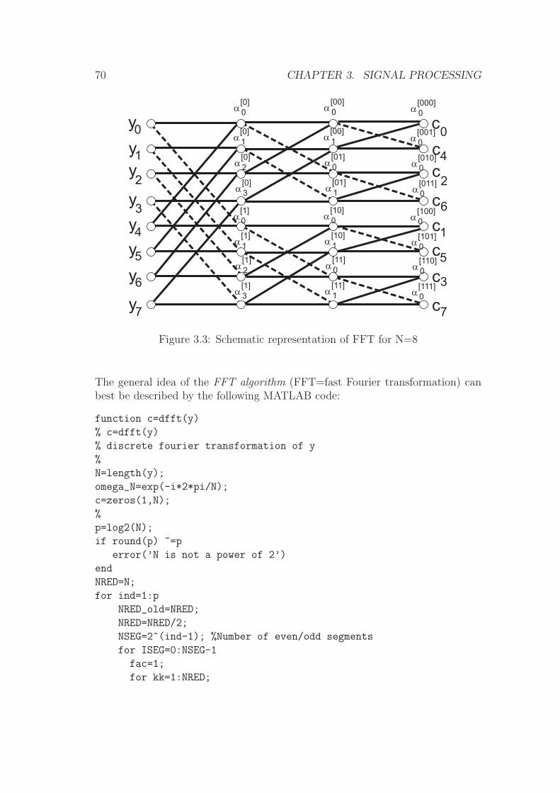
70 CHAPTER 3. SIGNAL PROCESSING
�
�
��
�
��
�
�
�
�
�
�
�
�
�
�
�
�
�
�
�
�����
�����
�����
�����
�����
�����
�����
�����
������
������
������
������
������
������
������
������
�������
�������
�������
�������
�������
�������
�������
�������
Figure 3.3: Schematic representation of FFT for N=8
The general idea of the FFT algorithm (FFT=fast Fourier transformation) canbest be described by the following MATLAB code:
function c=dfft(y)
% c=dfft(y)
% discrete fourier transformation of y
%
N=length(y);
omega_N=exp(-i*2*pi/N);
c=zeros(1,N);
%
p=log2(N);
if round(p) ~=p
error(’N is not a power of 2’)
end
NRED=N;
for ind=1:p
NRED_old=NRED;
NRED=NRED/2;
NSEG=2^(ind-1); %Number of even/odd segments
for ISEG=0:NSEG-1
fac=1;
for kk=1:NRED;

3.1. DISCRETE FOURIER TRANSFORMATION 71
k=kk+ISEG*NRED_old;
alpha_even=y(k)+y(k+NRED);
alpha_odd =(y(k)-y(k+NRED))*fac;
fac=fac*omega_N;
y(k)=alpha_even;
y(k+NRED)=alpha_odd;
end;
end;
omega_N=omega_N^2;
end;
% Sorting the indices and normalizing by N
% (this could be done by a simple bit-handling instead)
for j=0:N-1,
jbin=dec2bin(j,p+1);
jbininv=jbin(p+1:-1:2);
c(j+1)=y(bin2dec(jbininv)+1)/N;
end;

72 CHAPTER 3. SIGNAL PROCESSING
4090 4091 4092 4093 4094 4095 4096 4097 4098 409910
5
106
107
108
109
Number of Points
Flo
ps
Computational Effort for FFT in Dependency on Prime Factors
Prime Prime
2
2,5,409
2,3,11,31
2,23,89
3,5,7,13
17,241
2,3,683
Prime
Figure 3.4: Computational effort for FFT depending on the prime factors of N
The basic idea of this algorithm is due to Cooley and Tucker. It’s success is basedon the fact that it requires only O(N log2 N) multiplications if N is a power oftwo.If the number of samples N is no power of two, the iteration follows no longera binary tree and the sums (3.8) are split corresponding to the prime factors ofN . The computational works increases with the size of the prime factors and inthe extrem, when N is prime the computational effort becomes O(n2) which isjust the work which has to be done for the matrix-vector multiplication in (3.7),cf. Fig. 3.4.

Chapter 4
Iterative Methods
All methods we discussed so far were finite in nature, i.e. the result was obtainedin a finite number of computational steps. The computational effort for obtaininga numerical solution can be predicted, as the number of operation depends onlyon the problem type, not on the particular data. For example, to perform LU fac-torization of a non-sparse matrix requires always the same number of operations.If we assume that computations can be carried without any round-off error, thismethods would give the exact answer to the given problem in a finite numberof arithmetic operations (+,−, ·, /). However, that is an exceptional situation.In most cases solutions of mathematical problems can not be computed exactly.This is particularly the case, if the solution is a irrational number like
√2, for
example. Therefore, solutions of nonlinear equations, e.g.
x2 − 2 = 0
can not be computed exactly. As eigenvalues are defined as solutions of the char-acteristic polynomial, they are not computable in a finite number of operations.
The methods we will consider now are based on iterative processes. The nu-merical solution is the limit of a convergent series {xn}. Iteration means, thatone computes xi based on previous elements xi−1, xi−2, . . . and estimates the dis-tance ‖xi − x∗‖. If this quantity is small enough xi is taken as the numericalapproximation to the problem at hand. How many iterates it needs to reach thistolerance limit depends highly on the data. Consequently, the computationaleffort depends on the data and not only on the type of problem. Even assumingthat computations can be carried out at infinite precision (no round-off), theresult will be in general not the exact solution due to the truncation of the lim-iting process. We obtain only approximative solutions and we need a good errorestimation along with the method.
We discuss in this course iterative method to compute eigenvalues and zeros ofnonlinear functions.
73

74 CHAPTER 4. ITERATIVE METHODS
4.1 Computation of Eigenvalues
Recall the definition
Definition 77 Let A be a real n× n matrix, then λ ∈ C is called an eigenvalueof A if
det(A− λI) = 0.
If λ is an eigenvalue of a, then a vector x ∈ Cn is called a corresponding eigen-
vector of A ifAx = λx.
Furthermore we want to recall some basic properties of eigenvalues and eigenvec-tors
• An n× n matrix has n (not necessarily distinct) eigenvalues λ1, λ2, . . . , λn.
• If there are n linear dependent eigenvectors X = [x1, . . . , xn], then
X−1AX = diag(λ1, . . . , λn).
• If λ is an eigenvalue, than λ is also an eigenvalue of A.
• If A = AT than all eigenvalues are real. The eigenvectors are linear inde-pendent and form an orthogonal system, i.e. XXT = I.
• The eigenvalues of A are the zeros of its characteristic polynomial
p(λ) = det(A− λI)
It is a well-known result from algebra, that zeros only for polynomials up todegree 4 can be computed in a finite number of steps. So eigenvalues of matriceswith n ≥ 5 can only be computed iteratively and we will get only approximativeresults.Often, it is possible to estimate the location of the eigenvalues. For the methodswe discuss later in this section it is often sufficient to know in advance how theeigenvalues are clustered.A standard tool to get some a-priori information about the location of the eigen-values is the following theorem by Gerschgorin:
Theorem 78 Every eigenvalue λj ∈ C of the n × n matrix A is at least in oneof the circles
Bi :=
z ∈ C : |z − aii| ≤n∑
j=1
j �=i
|aij| =: ri
(4.1)

4.1. COMPUTATION OF EIGENVALUES 75
Proof :Let λ be an eigenvalue of A and x the corresponding eigenvector. Choose theindex i such that |xi| = ‖x‖∞. We write now the i-th component from the relationAx− λx = 0 as (
Ax)i= λxi.
Subtracting aiixi gives (Ax)i− aiixi = (λ− aii)xi.
Consequently,
|λ− aii| |xi| = |(Ax)i− aiixi| ≤
n∑j=1
j �=i
|aijxj| =n∑
j=1
j �=i
|aij| |xj| ≤( n∑
j=1
j �=i
|aij|)|xi|.
Thus λ ∈ Bi. ✷.
Furthermore it can be shown that if the union of r circles Bi is not intersectingthe remaining Bj, then the union contains exactly r eigenvalues.
4.1.1 Power iteration
We consider a symmetric N ×N matrix A. Let 0 �= x(0) ∈ RN be a given vector
and set
x(n) = Ax(n−1). (4.2)
Definition 79 The quantity
µ(n) :=x(n)TAx(n)
‖x(n)‖2 (4.3)
is called the Rayleigh quotient
We will relate now the Rayleigh quotient to the in modulus largest eigenvalue ofA:
Theorem 80 Let λ1, λ2, . . . , λN be the eigenvalues of A with |λ1| > |λi| and letx1 be the eigenvector corresponding to λ1. The iterates x(n) generated by therecursion (4.2) have the properties
limn→∞
µ(n) = λ1
if xT1 x
(0) �= 0.

76 CHAPTER 4. ITERATIVE METHODS
Proof :Let x1, . . . , xN be an orthonormal system of eigenvectors of A. Then, there arecoefficients αi such that
x(0) =N∑i=1
αixi.
Due to the orthogonality of the eigenvectors we get
xTi x
(0) = αi
and especially, by the assumption on x(0)
α1 �= 0.
Furthermore,
x(1) = Ax(0) =N∑i=1
αiAxi =N∑i=1
αiλixi
and by iterating
x(n) = Ax(n−1) = Anx(0) =N∑i=1
αiλni xi.
Due to the orthonormality of the xi:
x(n)Tx(n) = ‖x(n)‖22 =N∑i=1
α2iλ
2ni
and
x(n)TAx(n) =N∑i=1
α2iλ
2n+1i .
Thus,
µ(n) =
∑Ni=1 α
2iλ
2n+1i∑N
i=1 α2iλ
2ni
= λ1
∑Ni=1 α
2i
(λi
λ1
)2n+1∑Ni=1 α
2i
(λi
λ1
)2n .
As |λ1| > |λi| and α1 �= 0 we get
limµ(n) = λ1
✷
With mainly the same technique it can be shown
limn→∞
xTk x
(n)
‖x(n)‖ = 0 k = 2, 3, . . . , N (4.4)
which implies that x(n) converges towards the eigenvector x1.The iteration (4.2) is called power iteration. It is the simplest method to computethe largest eigenvalue and the corresponding eigenvector.We collect some properties of that iteration:

4.1. COMPUTATION OF EIGENVALUES 77
• The better the eigenvalues are separated the faster the convergence (seeexercises).
• If λ1 = λ2, then
limn→∞
xTk x
(n)
‖x(n)‖ = 0 k = 3, 4, . . . , N (4.5)
and x(n) converges no longer to an eigenvector, but
limn→∞
x(n) = x∗ ∈ span{x1, x2}.
Nevertheless, limµ(n) = λ1 = λ2
By power iteration we obtain the largest eigenvalue. The smallest eigenvaluecan be obtained by the inverse power iteration, which is based on the followingtheorem:
Theorem 81 Let λ be an eigenvalue of a regular n × n matrix A and x thecorresponding eigenvector. Then
• λ−1 is an eigenvalue of A−1 with eigenvector x
• λ− s is an eigenvalue of A− sI with eigenvector x.
So, if we apply the power iteration to A−1 we would obtain the largest eigenvalueof A−1 which is just the inverse of the smallest eigenvalue of A. This way ofapplying power iteration is called the inverse power iteration method.By applying the second statement of Theorem 81 enables us to compute alsoother eigenvalues, not only the largest or smallest. If we assume, that si is agood guess of the ith eigenvalue of A, then A − siI has an eigenvalue which isnear zero and consequently, we can expect, that (A − siI)
−1 has (λi − si)−1 as
its largest eigenvalue in modulus. Often Gerschgorin’s theorem can be applied toobtain a good guess for a certain eigenvalue. This technique to compute the ith
eigenvalue of A is called eigenvalue shift technique.The inverse power iteration is a good example for a problem, where the sameLU factorization is applied to many different right hand side vectors as we canrewrite the iteration in the following way in order to avoid direct inversion of A:
x(n) = A−1x(n−1) ⇔ Ax(n) = x(n−1).
Note, eigenvectors are unique up to scaling. The scaling factor tends to growduring the inverse iteration process. That is the reason, why the iterates arenormalized after each step.We summarize the algorithm for the inverse power iteration:
• Let x(0) be a given vector.

78 CHAPTER 4. ITERATIVE METHODS
• LU -factorize A (normally with pivoting)
• Solve Ax(1) = x(0) for x(1).
• Set x(1) := x(1)/‖x(1)‖
• Compute µ(1)
• Iterate these steps, i.e. Solve Ax(k) = x(k−1) for x(k), set x(k) := x(k)/‖x(k)‖and compute the Rayleigh quotient µ(k).
• If for some n the difference |µ(n) − µ(n−1)| is sufficiently small, then setλ = (µ(n))−1.
• Apply the eigenvalue shift to repeat the process for the next eigenvalue.
Recall that this algorithm is applied to symmetric matrices and that its con-vergence depends on how good the eigenvalues are separated from each other.The main application of this technique can be found in eigenvalue problems forboundary value problems, where depending on the particular discretization meth-ods symmetric matrices of the type (1.36) occur.There are also iteration methods for general, non symmetric matrices. Theseare based on an iterative similarity transformation of A to block triangular form(Schurform), cf. [Gv96].
4.2 Fixed Point Iteration
Fixed point iteration is the basis of nearly all iteration methods in NumericalAnalysis. The principle can be illustrated for a control circuit which has theproperties:
����
�� ���������� �
ϕ
������ ����
���������
Figure 4.1: Control circuit

4.2. FIXED POINT ITERATION 79
1. There is exactly one desired state x∗. Is the system in this state, thecontroler may not change anything
x∗ = ϕ(x∗).
In that sense, the desired state x∗ is called a fixed point of the controler ϕ.
2. The controler tries to reduce deviations from the desired state x∗
‖ϕ(x)− x∗‖ ≤ L‖x− x∗‖, L < 1 (4.6)
in order to stear the system towards x∗.
Formally speaking, such a control system is described by a fixed point iterationor functional iteration:
x(i) := ϕ(x(i−1)) (4.7)
with a given starting vector x(0).When applying an iteration scheme like (4.7) we have to ask ourselves the fol-lowing questions:
1. Are the iterates well defined ?
2. Do they converge ?
3. How fast do they converge ?
To answer these questions, more precise terminology is needed.
Definition 82 Let ϕ : D ⊂ Rn → R
n. We call a point x∗ ∈ D a fixed point ofϕ if
ϕ(x∗) = x∗ (4.8)
Fixed points and zeros of nonlinear functions are closely connected, as
F (x∗) = 0⇔ x∗ = x∗ − F (x∗) =: ϕ(x∗)
A fundamental property of the function ϕ is c.f. (4.6):
Definition 83 A function ϕ : D ⊆ Rn → R
n is called a contraction on a setD0 ⊆ D if there is an L(ϕ) < 1 and a norm such that
‖ϕ(x)− ϕ(y)‖ ≤ L(ϕ)‖x− y‖ (4.9)
for all x, y ∈ D0.Otherwise the function is called dissipative.

80 CHAPTER 4. ITERATIVE METHODS
Recall, that condition (4.9) implies that ϕ is Lipschitz continuous on D0.For differentiable functions, contractivity can be checked by applying the meanvalue theorem:
ϕ(x)− ϕ(y) =
∫ 1
0
ϕ′(x+ t(y − x))dt (x− y) (4.10)
In order to be able to apply this theorem we have to require
x, y ∈ D ⇒ x+ t(y − x) ∈ D ∀t ∈ [0, 1]
which implies that D has to be a convex set.Thus on convex sets D we then have
L(ϕ) = supx∈D‖ϕ′(x)‖. (4.11)
In this context it is important to relate norms to eigenvalues. Let us denote byρ(A) the absolute value of the largest eigenvalue of A. ρ(A) is sometimes calledthe spectral radius of A.
Theorem 84 For all An×n and all ε > 0 there exists a norm ‖.‖ such that
‖A‖ ≤ ρ(A) + ε
By this theorem and Eq. (4.11) we can check for continuously differentiablefunctions ϕ contractivity by checking eigenvalues:The condition
ρ(ϕ′(x∗)) ≤ δ < 1
is sufficient for ϕ being a contraction in a neighborhood of a point x∗.We are ready now for one of the most central theorems in Numerical Analysis
Theorem 85 (Fixed Point Theorem by Banach)Let ϕ : D ⊆ R
n → Rn be contractive on a closed set D0 ⊆ D and suppose
ϕ(D0) ⊂ D0.Then ϕ has a unique fixed point x∗ ∈ D0. Moreover for any arbitrary pointx(0) ∈ D0 the iteration x(i+1) = ϕ(x(i)) converges to x∗
Proof:For all x(0) ∈ D0 holds
‖x(i+1) − x(i)‖ = ‖ϕ(x(i))− ϕ(x(i−1))‖ ≤ L‖x(i) − x(i−1)‖ (4.12)
and consequently
‖x(i+1) − x(i)‖ ≤ Li‖x(1) − x(0)‖. (4.13)

4.2. FIXED POINT ITERATION 81
We show first that {x(i)} is a Cauchy-sequence:
‖x(i+m) − x(i)‖ ≤ ‖x(i+m) − x(i+m−1)‖+ · · ·+ ‖x(i+1) − x(i)‖≤ (Li+m + Li+m−1 + · · ·Li)‖x(1) − x(0)‖= Li(1 + L+ L2 + · · ·Lm−1)‖x(1) − x(0)‖≤ Li
1− L‖x(1) − x(0)‖.
Thus {x(i)} is a Cauchy series and as Rn is complete, there exists a x∗ ∈ R
n with
x∗ = limi→∞
x(i).
Furthermore as D0 is closed, x∗ ∈ D0. Now, we have to show that x∗ is a fixedpoint of ϕ:
‖x∗ − ϕ(x∗)‖ = ‖x∗ − x(i+1) + x(i+1) − ϕ(x∗)‖= ‖x∗ − x(i+1) + ϕ(x(i))− ϕ(x∗)‖≤ ‖x∗ − x(i+1)‖+ ‖ϕ(x(i))− ϕ(x∗)‖≤ ‖x∗ − x(i+1)‖︸ ︷︷ ︸
→0
+L ‖x(i) − x∗‖︸ ︷︷ ︸→0
Thus, x∗ = ϕ(x∗). ✷
We turn now to the question about the speed (rate) of convergence and aboutthe error we make, when we stop iterating after a finite number of iterations.Let x∗ be the fixed point. Then we get for contractive functions ϕ:
‖x(i) − x∗‖ = ‖ϕ(x(i−1))− ϕ(x∗)‖≤ L(ϕ)‖x(i−1) − x∗‖≤ L(ϕ)(‖x(i−1) − x(i)‖+ ‖x(i) − x∗‖)
(4.14)
and consequently:
‖x(i) − x∗‖ ≤ L(ϕ)
1− L(ϕ)‖x(i−1) − x(i)‖ (4.15)
This inequality is called an a posteriori error bound. With this we can decide onthe quality of the kth iterate after having computed it.If we want to know in advance how many iterates we would need to achieve acertain accuracy we apply an a priori error bound: Inserting
‖x(i−1) − x(i)‖ = ‖ϕ(x(i−2))− ϕ(x(i−1))‖ ≤ L(ϕ)‖x(i−2) − x(i−1)‖≤ L(ϕ)i−1‖x(0) − x(1)‖

82 CHAPTER 4. ITERATIVE METHODS
into (4.15) gives
‖x(i) − x∗‖ ≤ L(ϕ)i
1− L(ϕ)‖x(0) − x(1)‖ (4.16)
which is the desired a priori bound.
Definition 86 (Order or rate of convergence)An iteration is called convergent of order p, if
‖x(i) − x∗‖ ≤ C‖x(i−1) − x∗‖p
p is sometimes called also the rate of convergence.
Two special cases are of particular importance
• p = 2 quadratic convergence. We will see later that this is the ideal orderof convergence for Newton’s method.
• p = 1 linear convergence. As we see from (4.14), this is the order of con-vergence of fixed point iterations
Furthermore one often considers superlinear convergence which is achieved if theCk > 0 with
‖x(i) − x∗‖ ≤ Ci‖x(i−1) − x∗‖form a null sequence.
4.3 Newton’s Method
We consider now the problem:Find x ∈ R
n such that
F (x) = 0 (4.17)
with F : Rn → R
n.These kind of problems occur frequently in many technical applications, e.g. thedetermination of equilibrium points of dynamic processes in chemical, mechan-ical or electrical engineering. Furthermore, this problem occurs as a subtask inoptimization (the gradient has to be zero) and in other numerical methods, e.g.implicit discretization methods for ordinary differential equations.As usual we first recall what we know from calculus about the solvability of theproblem:
Theorem 87 (Inverse Function Theorem)Let F be continuously differentiable in an open set D ⊆ R
n and 0 ∈ F (D).Assume furthermore that F ′(x) regular for all x ∈ D, then

4.3. NEWTON’S METHOD 83
1. there is a locally unique x∗ ∈ Dwith F (x∗) = 0
2. there is in a neighborhood V (0) of 0a continuously differentiable function Gwith F (G(y)) = y and G(0) = x∗.
3. For the derivative the following relation holds in V (0):
G′(y) = (F ′(G(y)))−1
For the proof we refer to e.g. [OR70].We saw in the beginning of the preceding section how fixed point problems andthe problems of finding zeros of nonlinear functions are related. Fixed pointiteration applied to (4.17) might result in a slowly convergent or even divergentsequence x(i) depending on the contractivity of ϕ = I − F .We modify ϕ now so that(4.17) is equivalent to a fixed point problem with optimalcontractivity properties:
F (x) = 0⇐⇒ x = x− F ′(x)−1F (x) =: ϕN(x). (4.18)
Assume that F ′(x) is non singular in a neighborhood of x∗. Then
ϕ′N(x) = I −
(d
dxF ′(x)−1
)F (x)− F ′(x)−1F ′(x) = 0 at x = x∗.
Consequently, ϕN is contractive in a neighborhood of x∗.A fixed point iteration applied to ϕN(x) is Newton’s method for (4.17):
x(i+1) = x(i) − F ′(x(i))−1F (x(i)) =: ϕN(x(i))
In numerical computations however, the inverse of the Jacobian is never com-puted. Instead one solves a linear system. Therefore Newton’s method is betterdescribed by the following algorithmic notation:Newton’s method:Iterate the following two steps:
1. Solve the linear system F ′(x(i))∆x(i) = −F (x(i)) for ∆x(i).
2. Let x(i+1) := x(i) +∆x(i).
Obviously, every iteration step requires
• the computation of a Jacobian
• the solution of a linear system

84 CHAPTER 4. ITERATIVE METHODS
These high costs can only be compensated by a fast convergence. The conver-gence properties of Newton’s method are stated by the Newton–KantorovitchTheorem. It says that Newton’s method is locally quadratic convergent undersome conditions on the smootheness of F and on the topological properties ofD, i.e. for every x(0) sufficiently near the solution x∗ a sequence x(i) is generatedwith
‖x(i) − x∗‖ ≤ CN‖x(i−1) − x∗‖2.In many applications no information about the Jacobian F ′(x(i)) is available.Often F is known only as a set of complex subroutines, which are generated au-tomatically by special purpose programs in optimization or engineering. Thereare modern techniques, called automatic differentiation which generate a sub-routine for the corresponding Jacobian. These techniques can be viewed as apre-compiler1.
4.3.1 Numerical Computation of Jacobians
Alternatively, the Jacobian can be approximated by finite differences. The kth
column of the Jacobian is approximated by
∆ηekF =
F (x(i) + ηek)− F (x(i))
η
with ek being the kth unit vector and η ∈ R a sufficiently small number. Theincrement η has to be chosen such that the influence of the approximation errorε(η) can be neglected. It consists of truncation errors and roundoff errors inthe evaluation of F . Let εF be an upper bound for the error in the numericalcomputation of F , then
|εij(η)| =∣∣∣∣∆η
ejFi − ∂Fi
∂xj
∣∣∣∣ ≤ 2εF + 12‖∂2Fi
∂x2j‖η2 +O(η3)
η. (4.19)
In Fig. 4.2 the overall error for the example sin′(1) is given. In the left part ofthe figure the roundoff error dominates and in the right part the truncation error.The slopes in double logarithmic representation are -1 and +1 for the roundoffand approximation errors which can be expected from (4.19).When neglecting η2 and higher order terms this bound is minimized if η is selectedaccording the rule of thumb
η = 2
√εF
∣∣∣∣∂2Fi∂x2
j
∣∣∣∣−1
1see html://www.mcs.anl.gov/adifor

4.3. NEWTON’S METHOD 85
10−15
10−10
10−5
10010
−10
10−5
Perturbation η
Err
or |
ε(η)
|
Figure 4.2: Error |εij(η)| in the numerical computation of sin′(1)
which in practice is often replaced by
η = 2√εF .
The effort for the computation of F ′(x) by numerical differentiation consists ofaditional n additional evaluations of F . This high effort motivates the use ofsimplified Newton methods even when the convergence is no longer quadratic.Note that by numerically approximating F ′(x) this property is already lost (κ �=0).
4.3.2 Simplified Newton Method
In order to save evaluations of the Jacobian and to make full use of the first LUdecomposition, one may freeze the Jacobian in the first iteration step and iteratethe following two steps:
1. Solve the linear system F ′(x(0))∆x(i) = −F (x(i)) for ∆x(i).
2. Let x(i+1) := x(i) +∆x(i).
This method is called simplified Newton method. Every single step is much simplerto compute, because of the Jacobian and it’s LU factorization are already known.However this method is only linearly convergent.
Newton Convergence TheoremThe main theorem for the convergence of Newton’s method is the Newton Con-vergence Theorem, cf. [OR70, DH95]. We consider it here in a form, which is

86 CHAPTER 4. ITERATIVE METHODS
applicable also for the simplified Newton method (set in the theorem B(x) =F ′(x(0))−1 or for the Gauß-Newton method, which we will consider later (setB(x) = F ′(x)+).
Theorem 88Let D ⊂ R
n be open and convex and x(0) ∈ D.Let F ∈ C1(D,Rm) and B ∈ C0(D,Rn×m).Assume that there exist constants r, ω, κ, δ0 such that for all x, y ∈ D the followingproperties hold:
1. Curvature condition∥∥B(y)(F ′(x+ τ(y − x))− F ′(x)
)(y − x)
∥∥ ≤ τω ‖y − x‖2 (4.20)
with τ ∈ [0, 1].
2. Compatibility condition
‖B(y)R(x)‖ ≤ κ‖y − x‖ (4.21)
with the compatibility residual R(x) := F (x)−F ′(x)B(x)F (x) and κ < 1.
3. Contraction condition
δ0 := κ+ω
2‖x(1) − x(0)‖ < 1.
with x(1) = x(0) −B(x(0))F (x(0))
4. Condition on the initial guess
D0 :={x| ‖x− x(0)‖ ≤ r
}⊂Dwith r :=
‖x(1) − x(0)‖1− δ0
.
Then the iterationx(k+1) := x(k) −B(x(k))F (x(k))
is well-defined with x(k) ∈ D0 and converges to a solution x∗ ∈ D0 of B(x)F (x) =0.The speed of convergence can be estimated by
‖x(k+j) − x∗‖ ≤ δjk1− δk
‖∆x(k)‖ (4.22)
with δk := κ+ ω2‖∆x(k)‖ and the increments decay conforming to
‖∆x(k+1)‖ ≤ κ‖∆x(k)‖+ ω
2‖∆x(k)‖2. (4.23)

4.4. CONTINUATION METHODS IN EQUILIBRIUM COMPUTATION 87
By setting k = 0 the a priori error estimation formula
‖x(j) − x∗‖ ≤ δj01− δ0
‖x(1) − x(0)‖ (4.24)
can be obtained.This theorem with its constants needs some interpretation:
1. Curvature condition (1). This is a weighted Lipschitz condition for F ′,written in a way that it is invariant with respect to scaling. It can be fulfilledwith ω = L sup ‖B(y)‖ if F ′ is Lipschitz continuous with constant L and‖B‖ is bounded on D. For linear problems F ′ is constant and ω = 0. Then,the method converges in one step. Hence ω is a measure for the nonlinearityof the problem. In the case of a large ω, the radius of convergence r maybe very small because for a large ω, ‖x(1) − x(0)‖ has to be very small.
2. Compatibility condition (2). In the case of Newton’s method, i.e. B(x) =F ′(x)−1 we have R(x) = 0 and thus κ = 0. Then the method convergesquadratically.In the other cases this is a condition on the quality of the iteration matrixB(x). It says how tolerant we can be, when replacing F ′(x(k))−1 by anapproximate B(x). Due to κ �= 0 we can expect only linear convergence.The better the Newton iteration matrix is approximated the smaller κ.
3. “δ”-conditions (3), (4). These conditions are restrictions on the initialguess x(0). Newton’s method is only locally convergent and the size of theconvergence region depends on ω and κ.
4.4 Continuation Methods in Equilibrium Com-
putation
One of the main problems with Newton’s method is the choice of a starting valuex(0). In the case of highly nonlinear problems or due to a poor approximationB(x) of F ′(x)−1 the method might converge only for starting values x(0) in avery small neighborhood of the unknown solution x∗. So, special techniques forgenerating good starting values have to be applied. One way is to embed the givenproblem F (x) = 0 into a parameter depending family of problems H(x, s) = 0with
H(x, s) := F (x)− (1− s)F (x0) = 0 (4.25)
and a given value x0 ∈ D. This family contains two limiting problems. On onehand we have
H(x, 0) = F (x)− F (x0) = 0

88 CHAPTER 4. ITERATIVE METHODS
which is a system of nonlinear equations with x0 as a known solution. On theother hand we have
H(x, 1) = F (x) = 0
which is the problem we want to solve.The basic idea of continuation methods2 is to choose a partition 0 = s0 < s1 <s2 < · · · < sm = 1 of [0, 1] and to solve a sequence of problems
H(x, si) = 0, i = 1, . . . ,m
by Newton’s method where the solution xi of the ith problem is taken as startingvalue for the iteration in the next problem. The key point is that if ∆si = si+1−siis sufficiently small, then the iteration process will converge since the startingvalue xi for x will be hopefully in the region of convergence of the next subproblemH(x, si+1) = 0.From the mechanical point of view −F (x0) is a force which has to be added toF (x) in order to keep the system in a non-equilibrium position. The goal ofthe homotopy is then to successively reduce this force to zero by incrementallychanging s.The embedding chosen in (4.25) is called a global homotopy. It is a special caseof a more general class of embeddings, the so-called convex homotopy
H(x, s) := (1− s)G(x) + sF (x), s ∈ [0, 1] (4.26)
where G ∈ C1(D,Rn) is a function with a known zero, G(x0) = 0. By takingG(x) := F (x)− F (x0) the global homotopy is obtained again.We have
H(x, 0) = G(x), H(x, 1) = F (x),
i.e. the parameter s leads from a problem with a known solution to a problemwith an unknown solution. It describes a path x(s) with x(0) = x0 and x(1) = x∗.In general a homotopy function for a continuation method is defined as
H : Rn × R→ R
n
with H(x0, 0) = 0 and H(x, 1) = F (x), where x0 is a given point x0 ∈ D.The method sketched so far is based on the assumption that there exists a smoothsolution path x(s) without bifurcation and turning points. Before describing con-tinuation methods in more algorithmic details we look for criteria for an existenceof such a solution path.For this end we differentiate H(x(s), s) = 0 with respect to the parameter s andobtain
Hx(x, s)x′(s) = −Hs(x, s)
2Often also called homotopy or path following method.

4.4. CONTINUATION METHODS IN EQUILIBRIUM COMPUTATION 89
with Hx :=ddx
H, Hs :=ddsH.
If Hx(x, s) is regular we get to the so-called Davidenko differential equation:
x′(s) = −Hx(x, s)−1Hs(x, s), x(0) = x0 (4.27)
The existence of a solution path x(s) at least in a neighborhood of (x(0), 0) canbe ensured by standard existence theorems for ordinary differential equations aslong as Hx has a bounded inverse in that neighborhood. For the global homotopy(4.25) this requirement is met if F satisfies the conditions of the Inverse FunctionTheorem 87.For the global homotopy the Davidenko differential equation reads
x′(s) = −F ′(x)−1F (x0).
We summarize these observations in the following Lemma [AG90].
Lemma 89 Let H : D × I ⊂ Rn+1 → R
n be a sufficiently smooth map and letx0 ∈ R
n be such that H(x0, 0) = 0 and Hx(x0, 0) is regular.Then there exists for some open interval 0 ∈ I0 ⊂ I a smooth curveI0 ( s �→ x(s) ∈ R
n with
• x(0) = x0;
• H(x(s), s) = 0;
• rank(Hx(x(s), s)) = n ;
for all s ∈ I0.
The direction x′(s) given by the right hand side of the Davidenko differentialequation is just the tangent at the solution curve x in s.Fig. 4.3 motivates the following definition
Definition 90 A point (x(si), si) is called a turning point if rank(H′(x(si), si) =
n and rank(Hx(x(si), si)) < n.
In the neighborhood of turning points the curve cannot be parameterized by theparameter s and locally another parameterization must be taken into account.We not cover the topic of turning points in this course and refer to [AG90]instead. We will assume that there are no turning points in [0, 1].Having just seen that if no turning points are present, the path x(s) is just thesolution of an ordinary differential equation, the Davidenko differential equation,we could conclude this section by referring to numerical methods for ODEs. Un-fortunately, this differential equation cannot be solved in a stable way. Smallerrors are not damped out and will drift-off from the exact solution.

90 CHAPTER 4. ITERATIVE METHODS
x
s0 s1 si
ix'(s )
x(s)
Figure 4.3: Turning points
Most numerical path following methods are predictor-corrector methods. Thepredictor at step i provides a starting value x
(0)i for the Newton iteration which
attempts to “correct” this value to x(si) := x∗i .
We have already seen the predictor of the classical continuation method whichjust takes
x(0)i := x∗
i−1.
There, the predictor is just a constant function in each step.A more sophisticated predictor is used by the tangential continuation methodwhere the predictor is defined as
x(0)i := x∗
i−1 + (si − si−1)x′i−1(si).
This is just a step of the explicit Euler method for ODEs applied to the Davi-denko differential equation, cf. Sec. 5.7.1.
The amount of corrector iteration steps depends on the quality of the prediction.First, we have to require that the predicted value is within the convergence regionof the corrector problem. This region depends on the constants given by Theorem88, mainly on the nonlinearity of the F . Even if the predicted value is withinthe domain of convergence, it should for reasons of efficiency be such that thereare not too many corrector iteration steps needed. Both requirements demandan elaborated strategy for the step size control, i.e. for the location of the pointssi. For other strategies we refer to [AG90].A central example for an application of a homotopy method will be given in theproject homework of this course.

4.5. GAUSS-NEWTON METHOD 91
4.5 Gauß-Newton method
Consider the following example
Example 91 The radiation from a radioactive source is measured behind a pro-tective wall of thickness x as the number of counts per second. This number Ndepends on x according to theory in the following way:
N(x) = N0e−αx
Let us assume we want to determine the parameters α and N0 from n measure-ments N(xi), i = 1, . . . , n. If m > 2, then we get a nonlinear least squaresproblem. (Note, often logarithms are taken to transform it into a linear leastsquares problem, which might give a different solution!)
This problem is of the following general form:
‖F (x)‖22 = min
with F : Rn → R
m and m ≥ n.A necessary criterion forg(x) := F (x)TF (x) having a minimum is
g′(x) = 2G(x) = 2F ′(x)TF (x) = 0
The straight forward approach is to apply Newton’s method to G(x) = 0, whichgives the iteration
G′(x(k))∆x = −G(x(k)
with x(k) := x(k−1)) + ∆x. Note, that G′(x) =(ddx
F ′(x)T)F (x) + F ′(x)TF ′(x)
is the second derivative, the Hessian, of g. The numerical computation of thisfunction is time consuming and often not very reliable. This is why this approachis not very usefull. We will consider a second approach instead, which is basedon successively linearizing F and then minimizing.This way, we obtain a sequence of quadratic problems:
‖F (x(k)) + F ′(x(k))∆x‖22 = min
and set x(k+1) := x(k)) + ∆x. This method is called Gauß-Newton Method.Note, that we obtain in every iteration step a linear least squares problem withthe corresponding normal equations:
F ′(x(k))TF ′(x(k))∆x = −F ′(x(k))TF (x(k))
or expressed by the pseudo-inverse
∆x = −F ′(x(k))+F (x(k))

92 CHAPTER 4. ITERATIVE METHODS
which shows a formal similarity with Newton’s method for nonlinear equations.When comparing to the first approach, we note that we now neglected the Hes-sian. This neglection can be made if F (x∗) is sufficiently small, which correspondsto the requirement that the measurement errors are small and unbiased. In thatcase Newton’s convergence theorem assures locally linear convergence and in par-ticular if F (x∗) = 0 even locally quadratic convergence. For a detailed practicalexample see the exercises.
4.6 Iterative Methods for Linear Systems
We return in this section to the problem of solving linear systems of the form
Ax = b
where we assume that A ∈ Rn×n is regular. In Chapter 2 we considered so-called
direct methods, which computed the solution x in a finite number of computationsteps by some sort of factorization method. Here, we will consider iterativemethods for this problem, which approximate the solution within some givenaccuracy bound. In particular when the problem occurs as a subproblem fromsolving partial differential equations (PDEs)
• the dimension of A may be so large, that direct methods become to expen-sive,
• A often has a certain structure (sparsity pattern), which should be exploitedfor saving computation time and memory. This sparsity pattern often getslost when methods based on matrix factorization are applied. Zeros in thematrix are often replaced by non-zero elements by this process and thestructure of the matrix is destroyed. This effect is called fill-in.
• A is in this special application often a symmetric and even positive definite.So we will try to exploit this fact when considering iterative methods.
• PDEs are solved within some accuracy bound. The error depends on thedensity of the discretization mesh. It would be an unnecessary waste ofcomputation time to solve a subproblem, like linear system solving, to ahigher accuracy as the one required for the overall process.
All these points motivate the construction of iterative methods.We first reformulate the problem into a fixed point problem following the sameidea, which we applied when considering nonlinear problems, see p. 79:
Ax = b ⇔ Q−1(b− Ax) + x = x
(I −Q−1A)︸ ︷︷ ︸G
x+Q−1b︸ ︷︷ ︸c
= x

4.6. ITERATIVE METHODS FOR LINEAR SYSTEMS 93
where Q can be any regular n× n matrix.So we have to study the fixed point iteration for the problem
ϕ(x) = Gx+ c = x.
From the fixed point theorem (Th. 85) we conclude that the iteration
x(i+1) := Gx(i) + c
converges ifρ(G) < 1,
where ρ(G) denotes the spectral radius of G, see p. 80.We consider three important choices of Q:
• Q = I: Richardson iteration
• Q = D with Jacobi iteration
• Q = D + L with A = L+D + U : Gauss-Seidel iteration
Richardsson IterationIf we just choose Q = I we obtain the iteration
x(i+1) := x(i) − Ax(i) + b,
which converges if
ρ(G) = ρ(IA) = max{|1− λmax(A)|, |1− λmin|(A)} < 1
which is equivalent to |λ(A)| < 2. This restricts severely the class of problemsfor which this methods is applicable.
Jacobi IterationWe write A as a sum of a diagonal matrix D and lower and upper triangularmatrices L and U ,
A = L+D + U,
and choose Q = D. This gives the iteration
x(i+1) := −D−1(L+ U)x(i) +D−1b.
Again by checking the spectral radius we get a condition for convergence:
ρ(D−1(L+ U)) ≤ ‖D−1(L+ U)‖∞ = max∑i�=j|aijaii|
Thus, Jacobi iteration converges for diagonally dominant matrices.

94 CHAPTER 4. ITERATIVE METHODS
Gauss-Seidel IterationHere, we choose Q = D + L and obtain the iteration
x(i+1) := −(D + L)−1Ux(i) + (D + L)−1b.
As D + L is a triangular matrix one has to perform a forward substitution inevery iteration step.Gauss-Seidel iteration converges for all positive matrices A, see [DH95].

Chapter 5
Ordinary Differential Equations
In this chapter we want to compute numerically a function y ∈ C1[t0, te], whichis the solution of the following initial value problem
y = f(t, y) with y(t0) = y0. (5.1)
Initial value problems occur frequently in applications. The numerical solutionof these kind of problems is a central task in all simulation environments formechanical, electrical, chemical systems. There are special purpose simulationprograms for applications in these fields, which often require from their users adeep understanding of the basic properties of the underlying numerical methods.For constructing methods we might write this ordinary differential equation inintegral-form:
y(t) = y0 +
∫ t
t0
f(τ, y(τ)) dτ
Before we study numerical methods for computing a solution of (5.1) we haveto ask us the question if there exists a solution to that problem and if it isunique. Without existence and uniqueness guaranteed asking for a numericalsolution becomes obsolete. For this end let us review a central and basic resultsfrom ODE theory: The existence and uniqueness of a solution of (5.1) requireLipschitz continuity of f , i.e.
Definition 92 A function f : D ⊂ Rn → R
n is called Lipschitz continuous ifthere exists a constant L > 0 such that for all x, y ∈ D
‖f(x)− f(y)‖ ≤ L‖x− y‖For functions having this property we get the main theorem for initial valueproblems:
Theorem 93 (Picard and Lindelof)Let S := {(t, y)|t0 ≤ t ≤ te, y ∈ R
n} and let f : S → Rn be Lipschitz continuous
on S with respect to y, then there exists for every initial value (t0, y0) a uniquesolution y(t) of (5.1).
95

96 CHAPTER 5. ORDINARY DIFFERENTIAL EQUATIONS
5.1 Differential Equations of Higher Order
It is not necessarily always the first order derivative that appears in the differentialequation. The most prominent example of a second order differential equation isNewton’s law of mechanics
m · a(t) = f(x, t).
Here m is the mass of a body, a(t) = x(t) is its acceleration and f(t) is a forceacting on the body. If one is interested in the position as a function of time, thegoverning equation is the second order differential equation
x(t) = f(x, t)/m.
Introducing y1(t) = x(t) and y2(t) = x(t), the second order ODE can be rewrittenas a first order system of two equations:
y1(t) = y2(t),
y2(t) = x(t) = f(y1(t), t)/m.
In vector notation this system reads
Y (t) = F (t, Y (t)),
where Y =
(y1y2
)and F (t, Y ) =
(y2(t)
f(y1(t), t)/m
). Formally the solution is
given by “integration”
Y (t) = Y (t0) +
∫ t
t0
F (τ, Y (τ)) dτ.
Note that now the “initial value”
Y (t0) =
(y1(t0)y2(t0)
)=
(x(t0)x(t0)
)is a two component vector. In other words: To solve a second order ODE, twoinitial values need to be specified. Correspondingly, to solve a system of n 2nd.order ODEs 2n initial values are needed.
5.2 The Explicit Euler Method
The construction of numerical methods for initial value problems as well as basicproperties of such methods shall first be explained for the simplest method: Theexplicit Euler method. Be aware that this method is not the most efficient onefrom the computational point of view. In later sections, when a basic under-standing has been achieved, computationally efficient methods will be presented.

5.2. THE EXPLICIT EULER METHOD 97
5.2.1 Derivation of the Explicit Euler Method
A general principle to derive numerical methods is to “discretize” constuctionslike derivatives, integrals, etc.Given an initial value problem
y(t) = f(t, y(t)), y(t0) = y0
the operation which can not be evaluated numerically obviously is the limit h→ 0,that defines the derivative
y(t) = limh→0
y(t+ h)− y(t)
h.
However, for any positive (small) h, the finite difference
y(t+ h)− y(t)
h
can easily be evaluated. By definition, it is an approximation of the derivativey(t). Let us therefore approximate the differential equation y(t) = f(t, y(t)) bythe difference equation
u(t+ h)− u(t)
h= f(t, u(t)).
Given u at time t, one can compute u at the later time t + h, by solving thedifference equation
u(t+ h) = u(t) + hf(t, u(t)).
This is exactly one step of the explicit Euler method Introducing the notationtn+1 = tn + h and un = u(tn) it reads
un+1 = un + hf(tn, un), u0 = y0. (5.2)
We shall see in Sect. 5.4 that un really is a first order approximation to the exactsolution y(tn)
‖un − y(tn)‖ = O(h) h→ 0.
5.2.2 Graphical Illustration of the Explicit Euler Method
Given the solution y(tn) at some time tn, the differential equation y = f(t, y)tells us “in which direction to continue”. At time tn the explicit Euler methodcomputes this direction f(tn, un) and follows it for a small time step tn → tn+h.This is expressed in the formula (5.2) and illustrated in Fig. 5.1. Obviously eachstep introduces an error and ends up on a different trajectory. A natural question,that will be answered below is: How do these errors accumulate?

98 CHAPTER 5. ORDINARY DIFFERENTIAL EQUATIONS
0.8 1 1.2 1.4 1.6 1.8 2 2.2 2.40.7
0.75
0.8
0.85
0.9
0.95
1
1.05
1.1
1.15
1.2
t
y
Figure 5.1: Explicit Euler Method
5.2.3 Two Alternatives to Derive Euler’s Method
In the first derivation, the derivative was discretized using a finite differencequotient. This is not the only way to construct numerical methods for initial valueproblems. An alternative view on Euler’s method is based on the reformulationof the problem as an integal equation
y(t) = y0 +
∫ t
t0
f(τ, y(τ)) dτ
Then any of the quadrature rules of Chapter 1.4 can be applied to approximatethe integral. Choosing the rectangular rule,∫ tn+1
tn
f(τ, y(τ)) dτ ≈ hf(tn, y(tn)),
we find again Euler’s method
un+1 = un + hf(tn, un).
Clearly other quadrature rules will lead to other methods.Finally a constuction principle based on Taylor expansion shall be explained. Tothis end, one assumes that the solution of the initial value problem (5.1) can beexpanded in a Taylor series
y(tn + h) = y(tn) + hy(tn) +O(h2).

5.2. THE EXPLICIT EULER METHOD 99
Ignoring the second order term and using the differential equation to express thederivative y(tn) leads also to Euler’s method
un+1 = un + hf(tn, un).
5.2.4 Testing Euler’s Method
From the three derivations it is clear, that Euler’s method does not computethe exact solution of an initial value problem. All one can ask for is a reason-ably good approximation. The following experiment illustrates the quality of theapproximation. Consider the differential equation
y = −100y.
The exact solution is y(t) = y0e−100t. With a positive initial value y0 it is positive
and rapidly decreasing as t → ∞. The explicit Euler method applied to thisdifferential equation reads
un+1 = (1− 100h)un.
With a step size h = 0.1 the numerical “approximation” un+1 = −9un
un = (−9)nu0
oscillates with an exponentially growing amplitude. It does not approximatethe true solution at all. Reducing the step size to h = 0.001 however, yieldsun+1 = 0.9un and the numerical solution
un = (0.9)nu0
is smoothly decaying.
Another test example is the initial value problem
y = λ(y − sin(t)) + cos t, y(π/4) = 1/√2,
where λ is a parameter. First we set λ = −0.2 and compare the results forEuler’s method with two different step sizes h = π/10 and h = π/20, see Fig. 5.2.Obviously, the errors decrease with the step size. Setting now λ = −10 thenumerical results for h = π/10 oscillate arround the true solution and the errorsgrow rapidly in every single step. For the reduced step size h = π/20 however,Euler’s method gives a quite good approximation to the true solution, see Fig. 5.3.

100 CHAPTER 5. ORDINARY DIFFERENTIAL EQUATIONS
0.6 0.8 1 1.2 1.4 1.6 1.8 2 2.2 2.40.5
0.6
0.7
0.8
0.9
1
1.1
1.2
t
y
0.6 0.8 1 1.2 1.4 1.6 1.8 2 2.2 2.40.5
0.6
0.7
0.8
0.9
1
1.1
1.2
t
y
Figure 5.2: Explicit Euler Method, λ = −0.2, h = π/10 (left), h = π/20 (right)
0.6 0.8 1 1.2 1.4 1.6 1.8 2 2.2 2.40.5
0.6
0.7
0.8
0.9
1
1.1
1.2
t
y
0.6 0.8 1 1.2 1.4 1.6 1.8 2 2.2 2.40.5
0.6
0.7
0.8
0.9
1
1.1
1.2
t
y
Figure 5.3: Explicit Euler Method, λ = −10, h = π/10 (left), h = π/20 (right)
5.3 Stability Analysis
The previous section showed that in order to obtain reasonable approximationsthe step size in Euler’s method has to be choosen small enough — how smalldepends on the differential equation. The goal of the present section is to quantifythe condition on the step size. To this end consider the test equation
y = λy, (5.3)
where λ now is a complex parameter. The solution
y(t) = y0eλt
remains bounded|y(t)| = |y0| · |e(α+iβ)t| = |y0| · |eαt|

5.4. LOCAL, GLOBAL ERRORS AND CONVERGENCE 101
if α = Reλ is non positive. In this case it is reasonable to ask that the numericalsolution remains bounded too. For the explicit Euler method,
un+1 = (1 + hλ)un
this demand requires that the amplification factor is bounded by one
|1 + hλ| ≤ 1. (5.4)
The explicit Euler method is called stable for the test equation (5.3) if the stepsize h satisfies the condition (5.4). In the case of real and negative λ, this meansh ≤ −2/λ, cf. the experiments in the previous section.The set
S = {hλ ∈ C : |1 + hλ| ≤ 1}is called the stability region of the Euler method. It is a disc of radius 1 centeredat (−1, 0), see Fig. 5.4.
−2.5 −2 −1.5 −1 −0.5 0 0.5−1.5
−1
−0.5
0
0.5
1
1.5
Re
Im
Figure 5.4: Explicit Euler Method, stability region
5.4 Local, Global Errors and Convergence
So far qualitative properties of the approximation (boundedness, monotonicity)have been studied. In this section the actual errors will be analyzed. To this endwe have to destinguish local and global errors.
Definition 94 Given an initial value problem y = f(t, y) with y(0) = y0 andnumerical approximations un ≈ y(tn). The difference
en = un − y(tn)

102 CHAPTER 5. ORDINARY DIFFERENTIAL EQUATIONS
is called the global error. The difference
εn+1 = un+1 − y(tn+1)
is called the local error, where y is the solution to ˙y = f(t, y) with initial conditiony(tn) = un.
Note that the local error is an error in the numerical approximation, that is in-trocuced in one single time step; at time tn the values un and y(tn) are identical.The global error however, is an error at time tn that has accumulated duringn steps of integration. That is the error that one naturally observes when per-forming numerical calculation. In order to estimate the global error, we firstanalyze the local error and then study how local errors accumulate during manyintegration steps.Local errors can be analyzed by Taylor expansion. We demonstrate this for theexplicit Euler method
un+1 = un + hf(tn, un).
Inserting the initial condition for y yields
un+1 = y(tn) + hf(tn, y(tn)). (5.5)
Taylor expansion of y reads
y(tn+1) = y(tn) + h ˙y(tn) +h2
2¨y(tn) + . . .
Using the differential equation for y we find
y(tn+1) = y(tn) + hf(tn, y(tn)) +h2
2¨y(tn) + . . . (5.6)
Subtracting (5.6) from (5.5) gives the local error for the explicit Euler method :
εn+1 = −h2
2¨y(tn) + . . .
The accumulation of all local errors during the time stepping procedure deter-mines the global error which is observed after many iteration steps. To investigatethe global error, we subtract the Taylor expansion of the true solution
y(tn+1) = y(tn) + hy(tn) +h2
2y(tn) + . . .
= y(tn) + hf(tn, y(tn)) +h2
2y(tn) + . . .
from the explicit Euler method
un+1 = un + hf(tn, un).

5.5. STIFFNESS 103
This gives the global error recursion
en+1 = en + hf(tn, y(tn) + en)− hf(tn, y(tn))− εn+1 (5.7)
Taking norms and using Lipschitz–continuity of f yields
‖en+1‖ ≤ ‖en‖+ hLf‖en‖+ ‖εn+1‖.To get an explicit bound for ‖en‖, we apply the following result.
Lemma 95 (discrete Gronwall lemma) Let an+1 ≤ (1+hµ)an+b with h > 0,µ > 0, b > 0 and a0 = 0. Then
an ≤ b
h
etnµ − 1
µ, tn = nh.
For the global error we find the bound
‖en‖ ≤ hmax ‖y‖2
etnLf − 1
Lf.
For any fixed time level tn = nh, the global error decreases linearly with h :
‖en‖ = O(h) as h→ 0.
We say that Euler’s method is convergent of order 1. More precisely:
Definition 96 The order of convergence of a method is p, if the global errorsatisfies
‖en‖ = O(hp), h→ 0.
Note that the local error for Euler’s method is of second order ‖εn‖ = O(h2). Theaccumulation of local errors over n = O(h−1) steps causes the the order of theglobal error to decrease by one. The same effect was also observed for quadratureerrors in Section 1.4, c.f. Example 33. It is also interesting to compare the erroraccumulation in quadrature formulas, which consists in simply summing up localerrors, with the non–linear recursion (5.7).
5.5 Stiffness
The explicit Euler method is always stable for the test equation y = λy, λ < 0when only the step size h is small enough
h < −2/λ.However, for strongly negative λ* −1, this leads to extremely small step sizes.Small step sizes may be reasonable and hence acceptable if the right hand side

104 CHAPTER 5. ORDINARY DIFFERENTIAL EQUATIONS
of the differential equation is large and the solution has an large gradient. But,a stongly negative λ does not neccessarily imply large gradients (the right handside depends on y(t) also). Consider the example
y = λ(y − sin t) + cos t, λ = −50. (5.8)
A particular solution isyp(t) = sin t.
The general solution for the homogenous equation is
yh(t) = ceλt,
thus the general solution for the nonhomogenous differential equation (5.8) is
y(t) = (y0 − sin t0)eλ(t−t0) + sin t. (5.9)
This solution consists of a slowly varying part, sin t and an exponentially fastdecaying initial layer
(y0 − sin t0)eλ(t−t0).
Generally, differential equations which admit very fast initial layers as well asslow solution components, are called stiff problems.When in (5.9) y0 �= sin(t0) and λ* −1, then the layer has a large derivative andit is plausible that a numerical method requires small step sizes. However, afteronly a short time the initial layer has decayed to zero and is no longer visiblein the solution (5.9). Then y(t) ≈ sin t and it would be reasonable to use muchlarger time steps. Unfortunatelly, the explicit Euler method does not allow timesteps larger then the stability bound h < −2/λ. Even if we start the initial valueproblem for t0 = π/4 exactly on the slow component y0 = sin(π/4) —that meansthere is no initial layer present— the explicit Euler approximation diverges withh = 0.3 > −2/λ, see Fig. 5.5. The reason for this effect is as follows. In the firststep, the method introduces an local error as u1 �= sin(t1). Then in the secondstep the initial layer is activated, the step size is too large, and the error getsamplified.As it is impossible to avoid local errors, the only way out of this problem isis to construct methods with better stability properties. This leads to implicitmethods.
5.6 The Implicit Euler Method
Similar as for the explicit counterpart, there are several ways to derive the implicitEuler method. We begin by discretizing the derivative in y(t) = f(t, y(t)). Forsmall h it holds that
y(t)− y(t− h)
h≈ y(t) = lim
h→0
y(t)− y(t− h)
h,

5.6. THE IMPLICIT EULER METHOD 105
1 1.5 2 2.5 3−2
−1.5
−1
−0.5
0
0.5
1
1.5
2
time
solu
tion
Figure 5.5: Explicit Euler Method
thusy(t)− y(t− h)
h≈ f(t, y(t))
leading to the schemeun+1 = un + hf(tn+1, un+1). (5.10)
This method is known as the implicit Euler method. Given un ≈ y(tn), a newapproximation un+1 ≈ y(tn+1) is defined by formula (5.10). However, this is animplicit definition for un+1 and one has to solve the nonlinear equation (5.10) tocompute un+1. Clearly, the methods of Ch. 4 can be applied for that task. Forexample a fixed point iteration applied to (5.10)
u(j+1)n+1 = un + hf(tn+1, u
(j)n+1), j = 0, 2, . . .
is easy to compute once an initial guess u(0)n+1 is known. However, to find this
guess, which may be a rough approximation to un+1, an explicit Euler step isgood enough
u(0)n+1 = un + hf(tn, un).
In this context the explicit Euler step is called a predictor to the fixed point iter-ation which is then used as a corrector of the approximation. So called predictor–corrector algorithms will be discussed in more detail in Sect. 5.7.1.Before analyzing the implicit Euler method let us first give a second explanation.We have seen in Sec. 5.2.3 that numerical methods can also be derived from theintegral formulation of the initial value problem
y(t) = y0 +
∫ t
t0
f(τ, y(τ)) dτ.

106 CHAPTER 5. ORDINARY DIFFERENTIAL EQUATIONS
0.6 0.8 1 1.2 1.4 1.6 1.8 2 2.2 2.40.5
0.6
0.7
0.8
0.9
1
1.1
1.2
t
y
Figure 5.6: Implicit Euler Method
Approximating the integral by a rectangular rule where the integrand is evaluatedat the right end point of the integration intervall (instead of the left one),∫ tn+1
tn
f(τ, y(τ)) dτ ≈ h · f(tn+1, y(tn+1)),
we obtain again Euler’s implicit method
un+1 = un + hf(tn+1, un+1).
5.6.1 Graphical Illustration of the Implicit Euler Scheme
The implicit version of Euler’s method uses a numerical gradient in the n + 1st
step from tn to tn+1 which is equal to the gradient of the true solution in the newapproximation un+1:
un+1 − unh
= f(tn+1, un+1).
This is illustrated in Fig. 5.6.
5.6.2 Stability Analysis
The main motivation to search for implicit methods rather than explicit ones isto construct a more stable algorithm. Let us therefore check the stability of theimplicit version. Consider the test equation
y = λy
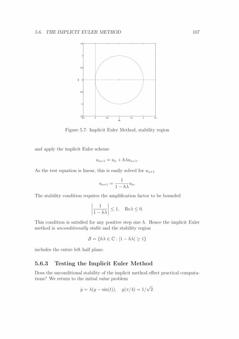
5.6. THE IMPLICIT EULER METHOD 107
−0.5 0 0.5 1 1.5 2 2.5−1.5
−1
−0.5
0
0.5
1
1.5
Re
Im
Figure 5.7: Implicit Euler Method, stability region
and apply the implicit Euler scheme
un+1 = un + hλun+1.
As the test equation is linear, this is easily solved for un+1
un+1 =1
1− hλun.
The stability condition requires the amplification factor to be bounded∣∣∣∣ 1
1− hλ
∣∣∣∣ ≤ 1, Reλ ≤ 0.
This condition is satisfied for any positive step size h. Hence the implicit Eulermethod is unconditionally stable and the stability region
S = {hλ ∈ C : |1− hλ| ≥ 1}
includes the entire left half plane.
5.6.3 Testing the Implicit Euler Method
Does the unconditional stability of the implicit method effect practical computa-tions? We return to the initial value problem
y = λ(y − sin(t)), y(π/4) = 1/√2.

108 CHAPTER 5. ORDINARY DIFFERENTIAL EQUATIONS
which could not be approximated by the explicit Euler method in the case λ =−10 and h = π/10, see Sect. 5.2.4.
Figs. 5.8 and 5.9 show a stable behaviour of the implicit method independentof the parameters λ and h. Also the errors obviously decrease as h → 0 (withλ fixed). In fact, the unconditionally stable implicit Euler method producesqualitatively correct approximations for all (reasonable) step sizes. Of course therobustness of the method has its price: solving a nonlinear equation in everysingle step.
0.6 0.8 1 1.2 1.4 1.6 1.8 2 2.2 2.40.5
0.6
0.7
0.8
0.9
1
1.1
1.2
t
y
0.6 0.8 1 1.2 1.4 1.6 1.8 2 2.2 2.40.5
0.6
0.7
0.8
0.9
1
1.1
1.2
t
y
Figure 5.8: Implicit Euler Method, λ = −0.2, h = π/10 (left), h = π/20 (right)
0.6 0.8 1 1.2 1.4 1.6 1.8 2 2.2 2.40.5
0.6
0.7
0.8
0.9
1
1.1
1.2
t
y
0.6 0.8 1 1.2 1.4 1.6 1.8 2 2.2 2.40.5
0.6
0.7
0.8
0.9
1
1.1
1.2
t
y
Figure 5.9: Implicit Euler Method, λ = −10, h = π/10 (left), h = π/20 (right)

5.7. MULTISTEP METHODS 109
5.7 Multistep Methods
5.7.1 Adams Methods
The idea leading to Adams methods is quite simple. It is based on transformingthe initial value problem
y = f(t, y) with y(t0) = y0 (5.11)
into its integral form
y(t) = y0 +
∫ t
t0
f(τ, y(τ)) dτ (5.12)
and then approximating the integrand by an adequate polynomial. We will as-sume that the time interval under consideration is partitioned into
t0 < t1 < · · · < ti < ti+1 = ti + hi < · · · < te
with the step size hi at step i+1. Let us assume for the moment that k solutionpoints at successive time points are given
un+1−i := y(tn+1−i), i = 1, . . . , k.
Then, by evaluating the function to be integrated (right hand side function in(5.11) or simply rhs-function) the corresponding derivatives
f(tn+1−i, y(tn+1−i)), i = 1, . . . , k
are known and can be used to define an interpolation polynomial πpk of degree
k − 1 with the property
πpk(tn+1−i) = f(tn+1−i, un+1−i), i = 1, . . . , k.
By this requirement this polynomial is uniquely defined, though there are manydifferent ways to represent it. For theoretical purposes the Lagrange formulationis convenient. There, πp
k is combined of Lagrange basis polynomials Lk−1i (t) (cf.
Sec. 1.2.1 and Sec. 1.4)
πpk(t) =
k∑i=1
Lk−1i (t)f(tn+1−i, un+1−i) (5.13)
with
Lk−1i (t) :=
k∏i�=j=1
t− tn+1−jtn+1−i − tn+1−j
.
They fulfill
Lk−1i (tn+1−j) := δij (Kronecker symbol).

110 CHAPTER 5. ORDINARY DIFFERENTIAL EQUATIONS
By integrating (5.13) from tn to tn+1, the Adams–Bashforth scheme in Lagrangeformulation for approximating y(tn+1) is obtained:
upn+1 = un + hn
k∑i=1
βpk−if(tn+1−i, un+1−i) (5.14)
with βpk−i =
1
hn
∫ tn+1
tn
Lk−1i (t) dt.
The number of previous values needed to approximate x(tn+1) is called the num-ber of steps of the method and all previous values and their derivatives sometimesare called the trail of the method. In the sequel we will denote by un the numericalapproximation to y(tn) and set fn := f(tn, un).
Example 97 For equal (constant) step sizes the Adams–Bashforth methods aregiven by the following formulas
k = 1 : un+1 = un + hfn explicit Euler method
k = 2 : un+1 = un + h(32fn − 1
2fn−1
)k = 3 : un+1 = un + h
(2312fn − 16
12fn−1 +
512fn−2
).
As a consequence of the construction of the basic polynomials Lk−1i the coefficients
β depend on the spacings hn, . . . , hn−k. In practical codes the polynomials arenormally not represented by Lagrange polynomials. For computational efficiencya modified Newton representation is taken instead, cf. Eq. (1.5). To improve thestability of the method an implicit multistep scheme is taken into consideration:Let us assume for the moment that un+1 and previous values are known. Then apolynomial πc
k+1 of degree k can be constructed by requiring
πck+1(tn+1−i) = f(tn+1−i, un+1−i), i = 0, 1, . . . , k.
Similar to Eq. (5.14) this leads to the so-called Adams–Moulton method :
un+1 = un + hn
k∑i=0
βck−if(tn+1−i, un+1−i) (5.15)
with
βck−i :=
1
hn
∫ tn+1
tn
Lki (t) dt
Lki (t) :=k∏
i�=j=0
t− tn+1−jtn+1−i − tn+1−j
.

5.7. MULTISTEP METHODS 111
Example 98 For equal (constant) step sizes the Adams–Moulton methods aregiven by the following formulas
k = 0 : un+1 = un + hfn+1 implicit Euler method
k = 1 : un+1 = un + h(12fn+1 +
12fn)
Trapezoidal rule
k = 2 : un+1 = un + h(
512fn+1 +
812fn − 1
12fn−1
)k = 3 : un+1 = un + h
(924fn+1 +
1924fn − 5
24fn−1 +
124fn−2
).
In contrast to Eq. (5.14) Adams–Moulton methods are defined by implicit equa-tions, which must be solved iteratively for un+1. The iteration process is startedwith the “predicted” value up
n+1 from the Adams–Bashforth scheme (5.14).This results in the Adams Predictor-Corrector scheme:
Predict (P)
upn+1 = un + hn
∑ki=1 β
pk−if(tn+1−i, un+1−i)
Evaluate (E)
f(tn+1, upn+1)
Correct (C)
un+1 = un + hn
(βckf(tn+1, u
pn+1) +
∑ki=1 β
ck−if(tn+1−i, un+1−i)
)Evaluate (E)
f(tn+1, un+1).
(5.16)
This scheme is symbolized by the abbreviation PECE. Frequently, the correctoris iterated in the following way:
u(i+1)n+1 = un + hn
(βckf(tn+1, u
(i)n+1) +
k∑i=1
βck−if(tn+1−i, un+1−i)
)i = 0, . . . ,m− 1
(5.17)
with u(0)n+1 := up
n+1. This implementation is symbolized by P (EC)mE. It con-sists of m steps of a fixed point iteration. The integration step is completed byassigning un+1 := u
(m)n+1. Though the scheme (5.15) is an implicit one, the overall
method is explicit if there is only a fixed number of corrector iteration steps taken,e.g. m = 1. Alternatively, this iteration can be carried out “until convergence”,i.e. the iteration is controlled and m is kept variable. These versions differ withrespect to their stability properties. In the sequel we will assume always correctorvalues obtained from iterating until convergence unless otherwise stated.

112 CHAPTER 5. ORDINARY DIFFERENTIAL EQUATIONS
5.7.2 Backward Differentiation Formulas (BDF)
There is another important class of multistep methods, which is based on in-terpolating the solution points un+1−i rather than the derivatives. Let πp
k be apolynomial of degree (k − 1), which interpolates the k points
un+1−i, i = 1, . . . , k.
Again, using the Lagrange formulation it can be expressed by
πpk(t) =
k∑i=1
Lk−1i (t)un+1−i.
By just extrapolating this polynomial, a new solution point can be predicted as
xpn+1 = πp
k(tn+1) =k∑i=1
Lk−1i (tn+1)un+1−i.
Introducing the coefficients αpk−i := −Lk−1
i (tn+1) the predictor equation
upn+1 = −
k∑i=1
αpk−iun+1−i
is obtained. In this formula no information about the function f is incorporated.It is only useful as a predictor in a predictor–corrector scheme. The BDF correctorformula is obtained by considering the kth degree polynomial πc
k+1 which satisfiesthe conditions:
πck+1(tn+1−i) = un+1−i, i = 0, . . . , k (5.18a)
πck+1(tn+1) = f(tn+1, un+1). (5.18b)
The first conditions are interpolation conditions using the unknown value xn+1,which is defined implicitly by considering (5.18b).With the coefficients
αck−i :=
Lki (tn+1)
Lk0(tn+1), βc
k :=1
hnLk0(tn+1)
equation (5.18b) can be expressed by
un+1 = −k∑i=1
αck−iun+1−i + hnβ
ckf(tn+1, un+1), (5.19)
where the Lki now correspond to the interpolation points un+1−i, i = 0, . . . , k.This is the corrector scheme of the backward differentiation formula. We will see

5.7. MULTISTEP METHODS 113
later that this method is of particular interest for stiff problems. The predictor-corrector scheme for a BDF method has the form:
Predict (P)
upn+1 = −
∑ki=1 α
pk−iun+1−i
Evaluate (E)
f(tn+1, upn+1)
Correct (C)
un+1 = −∑k
i=1 αck−iun+1−i + hnβ
ckf(tn+1, u
pn+1)
(5.20)
Again, the implicit formula can be solved iteratively by applying the schemeP (EC)m with m ≥ 1, though, in practice, BDF methods are mainly implementedtogether with Newton’s method. We will see the reason for this later, whendiscussing stiff ODEs.
5.7.3 Solving the Corrector Equations
In this section we discuss the corrector iteration. The corrector iteration describedso far has the general form
u(i+1)n+1 = ξ + hnβ
ckf(tn+1, u
(i)n+1) (5.21)
with ξ being the contributions based on “old” data, which is
ξ = un + hn
k∑i=1
βck−if(tn+1−i, un+1−i)
in the case of Adams–Moulton methods, see Eq. (5.17), and
ξ = −k∑i=1
αck−iun+1−i
in the case of implicit BDF methods, cf. (5.20). Eq. (5.21) describes a fixed pointiteration. By the fixed point theorem a necessary condition for the convergenceof this iteration is that the corresponding mapping
ϕ(u) = ξ + hnβckf(t, u)
is a contraction, cf. Def. 4.9. As the Lipschitz constants of ϕ and f are relatedby
L(ϕ) = hn|βck|L(f),

114 CHAPTER 5. ORDINARY DIFFERENTIAL EQUATIONS
it is obvious that ϕ is contractive and the iteration convergent if the step sizeis sufficiently small. In many cases L(f) is of moderate size such that the stepsize for the required local accuracy is small enough to ensure fast convergenceof the fixed point iteration. On the other hand, if the Jacobian d
dxf(t, x) has
eigenvalues being large in modulus, the step size might be restricted much moreby the demand for contractivity than by the required tolerance and stability.This situation is to be expected when dealing with stiff systems. In this case it isappropriate to switch from fixed point iteration to Newton iteration for solvingthe implicit corrector equation. When applying Newton’s method, the nonlinearequation
F (un+1) = un+1 − (ξ + hnβckf(tn+1, un+1)) = 0 (5.22)
is considered. Newton’s method then defines the iteration
J(tn+1, u(i)n+1)∆u(i) = −
(u(i)n+1 − (ξ + hnβ
ckf(tn+1, u
(i)n+1))
)(5.23)
with u(i+1)n+1 := u
(i)n+1 +∆u(i) and
J(t, u) := I − hβck
d
duf(t, u).
Like in the case of fixed point iteration the predictor solution is taken as startingvalue: u
(0)n+1 := up
n+1. The method demands an high computational effort, whichis mostly spent when computing the Jacobian J and solving the linear system.
5.7.4 Order Selection and Starting a Multistep Method
The local residual of a pth order method depends on the p+ 1st derivative of thesolution in the actual time interval [tn, tn+1]. If
‖cphpy(p)‖ < ‖cp+1hp+1y(p+1)‖
it might be advantageous to take a method of order p − 1 instead. Similarly,one might consider to raise the order if the higher derivative is smaller in thatsense. Adams and BDF methods allow to vary the order in an easy way. Theyare defined in terms of interpolation polynomials based on a certain number ofpoints. Raising or lowering the number of interpolation points raises or lowers theorder of the interpolation polynomial and the order of the method. After everysuccessful step it is considered how many points of the past should be takento perform the next step. As mentioned earlier in this chapter, interpolationpolynomials can be defined in different ways. Especially the definition based onfinite differences, like in Newton’s interpolation method, permits in an efficientway to vary the order of an interpolation polynomial by adding or taking awayadditional interpolation points. In order to get an idea of the size of y(p+1), thepth resp. p + 1st derivative of the kth order interpolation polynomial is taken.

5.8. EXPLICIT RUNGE–KUTTA METHODS 115
The automatic order variation is also used for starting multistep methods: Thestarting points are successively obtained by starting with a one step method, thenproceeding with a two step method and so on until an order is reached which isappropriate for the given problem.
5.8 Explicit Runge–Kutta Methods
Runge–Kutta methods are one-step methods, i.e. they have the generic form
un+1 := un + hφh(tn, un) (5.24)
with a method dependent increment function φh. In contrast to multistep meth-ods, the transition from one step to the next is based on data of the most recentstep only.The basic construction scheme is
U1 = un (5.25a)
Ui = un + hi−1∑j=1
aijf(tn + cjh, Uj) i = 2, . . . , s (5.25b)
un+1 = un + hs∑i=1
bif(tn + cih, Ui). (5.25c)
s is called the number of stages.
Example 99 By taking s = 2, a21 = 1/2, b1 = 0, b2 = 1, c1 = 0, and c2 = 1/2 thefollowing scheme is obtained
U1 = un (5.26a)
U2 = un +h
2f(tn, U1) (5.26b)
un+1 = un + hf(tn +h
2, U2) (5.26c)
For this method the increment function reads
φh(t, u) := f(t+
h
2, u+
h
2f(t, u)
).
Normally, Runge–Kutta methods are written in an equivalent form by substitut-ing ki := f(tn + cih, Ui)
k1 = f(tn, un)
ki = f(tn + cih, un + h
i−1∑j=1
aijkj) i = 2, . . . , s
un+1 = un + hs∑i=1
biki.

116 CHAPTER 5. ORDINARY DIFFERENTIAL EQUATIONS
The coefficients characterizing a Runge–Kutta method are written in a compactform using a so-called Butcher tableau:
c1c2 a21c3 a31 a32...
......
. . .
cs as1 as2 · · · as,s−1
b1 b2 · · · bs−1 bs
orc A
bT
with A = (aij) and aij = 0 for j ≥ i.The classical 4-stage Runge–Kutta method reads in this notation
012
12
12
0 12
1 0 0 116
26
26
16
. (5.27)
An s-stage Runge–Kutta method usually requires s function evaluations. If
cs = 1, asj = bj and bs = 0 (5.28)
the function evaluation for the last stage at tn can be used for the first stage attn+1.The higher amount of function evaluations per step in Runge–Kutta methodscompared to multistep methods is often compensated by the fact that Runge–Kutta methods may be able to use larger step sizes.A non autonomous differential equation y = f(t, y) can be written in autonomousform where the right hand side of the differential equation is not explicitly de-pending on time, by augmenting the system by the trivial equation t = 1:
y =
(tx
)=
(1
f(t, x)
)= F (y).
Applying a Runge–Kutta method to the original and to the reformulated systemshould lead to the same equations. This requirement relates the coefficients ci tothe aij:
ci =s∑j=1
aij. (5.29)
We will consider only methods fulfilling this condition and assuming for the restof this chapter autonomous differential equations for ease of notation.

5.8. EXPLICIT RUNGE–KUTTA METHODS 117
5.8.1 The Order of a Runge–Kutta Method
The global error of a Runge–Kutta method at tn is defined in the same way asfor Euler’s method
en := y(tn)− un.
with n = tn/h. A Runge–Kutta method has order p if en = O(hp).Using (5.24) we get
en+1 = y(tn+1)− un − hφh(tn, un)
= y(tn+1)− y(tn) + en − h(φh(tn, y(tn))− φh(tn, y(tn)) + φh(tn, un)).
Setting ε(t, y, h) := y(t + h) − y(t) − hφh(t, y(t)) and applying the mean valuetheorem1 to φ gives
en+1 = Φn(h)en + ε(tn, y, h) +O(e2n) (5.30)
with Φn(h) := 1 + h ddyφh(tn, y)
y(tn). Thus,
Φn(h) = 1 +O(h).
ε is called the local error or, due to its role in (5.30), the global error incrementof the Runge–Kutta method.Viewing the error propagation formula (5.30) we have to require
ε(tn, y, h) = O(hp+1) (5.31)
to get a method of order p.
Example 100 For the Runge–Kutta method (5.26) we get by Taylor expansion
ε(tn−1, y, h) =h3
24(fyyf
2 + 4f 2y f) +O(h4). (5.32)
using the notation fy :=ddyf(y)
y(tn−1)for the elementary differentials.
Thus (5.26) is a second order method.
The goal when constructing a Runge–Kutta method is to choose the coefficients insuch a way that all elementary differentials up to a certain order cancel in a Taylorseries expansion of ε. This requires a special symbolic calculus with elementarydifferentials, which is based on relating these differentials to labeled trees. Theorder conditions are much more complicated than in the multistep case. Theyconsist of an underdetermined system of nonlinear equations for the coefficientsA, b, c, which is solved by considering additional simplifying assumptions.
1For notational simplicity we restrict the presentation to the scalar case.

118 CHAPTER 5. ORDINARY DIFFERENTIAL EQUATIONS
5.8.2 Embedded Methods for Error Estimation
Variable step size codes adjust the step size in such a way, that the global errorincrement is kept below a certain tolerance threshold TOL. This requires agood estimation of this quantity. The error can be estimated by comparing twodifferent methods. Here, a Runge–Kutta method of order p and another methodof order p+ 1 is taken to perform a step from tn to tn+1, say.The local error of the pth order method is
ε(p)(t, y) = C(p)(t, y)hp+1 +O(hp+2)
while the global error increment of the p+ 1st order method is
ε(p+1)(t, y) = C(p+1)(t, y)hp+2 +O(hp+3),
where the coefficients C(i) depend on error coefficients and elementary differen-tials, cf. (5.32).The difference of both quantities is
u(p)n − u(p+1)
n = C(p)(t, y)hp+1 +O(hp+2) = ε(p)(tn, y(tn)) +O(hp+2)
where the superscripts indicate the respective method.Directly evaluating this formula for estimating the error would require addi-tional function evaluations according to the number of stages of the higher ordermethod. This would be much too expensive. This extra work can be avoidedby using embedded methods. These are pairs of Runge–Kutta methods using thesame coefficients A and c. Thus, the stage values ki of both methods coincide.The only difference is in the b coefficients, which are determined in such a way,that one method has order p + 1 while the other has order p. The two methodsare described by the tableau
c1c2 a21c3 a31 a32...
......
...cs as1 as2 · · · as,s−1
bp1 bp2 · · · bps−1 bps
bp+11 bp+1
2 · · · bp+1s−1 bp+1
s
where p indicates the order of the method and where
u(p)n+1 = un + h
s∑i=1
bpi ki
u(p+1)n+1 = un + h
s∑i=1
bp+1i ki.

5.8. EXPLICIT RUNGE–KUTTA METHODS 119
Example 101 One method of low order in that class is the RKF2(3) method
01 112
14
14
12
12
016
16
46
(5.33)
It uses 3 stages and is due to Fehlberg.
Local ExtrapolationThough it is always the error of the lower order method which is estimated,one often uses the higher order and more accurate method for continuing theintegration process. This foregoing is called local extrapolation. This is alsoreflected in naming the method, i.e.
• in RK2(3) the integration process is carried out with a second order methodand in
• in RK3(2) local extrapolation is used, thus a third order method is takenfor the integration.
When designing a Runge–Kutta method one is interested in minimizing theweights in the principle error term. In the context of embedded methods thedifference of both methods must be as large as possible to give a good estimate,so it might not be a good idea to seek for a lower order method with minimalweights in the principle error term, when applying local extrapolation. Coeffi-cients optimal with respect to this and some other design criteria have been foundby Dormand and Prince leading to one of the most effective explicit Runge–Kuttaformulas. We give here the coefficients for the 5,4-pair:
Example 102
015
15
310
340
940
45
4445
−5615
329
89
193726561
−253602187
644486561
−212729
1 90173168
−35533
467325247
49176
− 510318656
1 35384
0 5001113
125192
−21876784
1184
35384
0 5001113
125192
−21876784
1184
0
517957600
0 757116695
393640
− 92097339200
1872100
140
(5.34)

120 CHAPTER 5. ORDINARY DIFFERENTIAL EQUATIONS
This method uses six stages for 5th order result and one more for obtaining the4th order result. One clearly sees that the method saves one function evaluationby meeting the requirement (5.28) for the 5th order method which is used for localextrapolation.
5.8.3 Stability of Runge–Kutta Methods
Similar to the discussion for Euler’s method, we investigate the stability of Runge–Kutta methods for finite step sizes h by considering the linear test equationy = λy, cf. Sect. 5.3Applying the Runge–Kutta method (5.25) to that equation results in
U1 = un
Ui = un + h
i−1∑j=1
aijλUj i = 2, . . . , s
un+1 = un + h
s∑i=1
biλUi.
By inserting the stage values into the final equation we get
un+1 =(1 + hλ
s∑i=1
bi + (hλ)2s∑i=2
biai1 + (hλ)3s∑i=3
biai2ai−1,1 + . . .
. . .+ (hλ)sbsas,s−1 · as−1,s−2 . . . a2,1
)un
:= R(hλ)un. (5.35)
The function R : C→ C is called stability function of the Runge–Kutta method,see also the amplification factor (5.4) for Euler’s method.A Runge–Kutta method is stable for a given step size h and a given complexparameter λ if |R(hλ)| ≤ 1. Then, an error in y0 is not increased by applying(5.35).In Fig. 5.10 the stability regions of the methods DOPRI4 and DOPRI5 are dis-played. One realizes that lower order methods tend to have the larger stabilityregion. When applying embedded methods with local extrapolation this factmust be envisaged.

5.8. EXPLICIT RUNGE–KUTTA METHODS 121
-4 -2 0 2-4
-2
0
2
4
DOPRI4
DOPRI5
Figure 5.10: Stability regions for the Runge–Kutta pair DOPRI4 and DO-PRI5.The methods are stable inside the gray areas.

122 CHAPTER 5. ORDINARY DIFFERENTIAL EQUATIONS

Bibliography
[AG90] Eugene L. Allgower and Kurt Georg. Numerical Continuation Meth-ods. Springer, 1990.
[BB99] Adrian Biran and Moshe Breiner. MATLAB 5 for Engineers.Addison-Wesley, 1999.
[de 78] C. de Boor. A practical guide to splines. Springer-Verlag, 1978.
[DH95] Peter Deuflhard and Andreas Hohmann. Numerical Analysis - A firstcourse in Scientific computing. Walter de Gruyter, 1995.
[Far88] Gerald Farin. Curves and Surfaces in Computer Aided GeometricDesign. New York, 1988.
[Gv96] Gene H. Golub and Charles F. van Loan. Matrix Computations. JohnHopkins University Press, 3rd edition, 1996.
[GW99] Curtis F. Gerald and Patrick O. Wheatley. Applied Numerical Anal-ysis. Addison-Weseley, 6th edition, 1999.
[Hea97] Michal T. Heath. Introduction to Scientific Computing. McGrawHill, 1997.
[Jam95] John F. James. A Student’s Guide to Fourier Transforms. CambridgeUniversity Press, 1995.
[OR70] J.M. Ortega and W.C. Rheinboldt. Iterative Solutions of NonlinearEquations in Several Variables. Academic Press, New York, 1970.
[PESMI96] Eva Part-Enander, Anders Sjoberg, Bo Melin, and Pernilla Isaksson.The MATLAB Handbook. Addison-Wesley, 1996.
[QSS00] Alfio Quarteroni, Riccardo Sacco, and Fausto Saleri. NumericalMathematics. Springer, 2000.
[SAP97] Lawrence Shampine, Richard Allen, and Steve Pruess. Fundamentalsof Numerical Computing. John Wiley, 1997.
[Spa94] Gunnar Sparr. Linjar algebra. Studentlitteratur, 1994.
123

Index
p-norm, 49
singular values, 62
a posteriori error bound, 81a priori error bound, 81Adams method, 109Aitken, 8amplification factor, 101automatic differentiation, 84autonomous ODE, 116
B-splines, 37Bezier curve
partial, 16Bezier points, 12backward differentiation formula, 112backward substitution, 43barycentric combinations, 13BDF, 113Bernstein polynomials, 11boundary conditions, 32Butcher tableau, 116
characteristic polynomial, 74Chebychev points, 22Chebyshev-Polynomials , 20complete pivoting, 47complex trigonometric polynomials,
63condition number, 51continuation methods, 88contraction, 113contraction, 79convergence
Newton’s method, 85convergent of order p, 82
convex combinations, 13convex set, 80Cooley, 72corrector
Adams method, 111BDF method, 112Euler method, 105solution, 113
Davidenko differential equation, 89de Boor points, 39de Casteljau algorithm, 15diagonal row dominant, 46Discrete Fourier tranformation, 65dissipative, 79divided differences, 8
eigenvalue, 74eigenvector, 74elementary transformation matrices,
44elementary transformation matrix, 44embedded methods, 118explicit Euler
amplification factor, 101convergence, 103global error, 103local error, 102method, 97stability region, 101
FFT algorithm, 70fill-in, 92fixed point, 79fixed point iteration, 79flop, 44
124

INDEX 125
forward substitution, 43functional iteration, 79
Gauss-methods, 29Gauss-Seidel iteration, 93Gauß methods, 31Gauß-Newton Method, 91Gerschgorin, 74global error, 102global error increment, 117
Holder-norm, 49homotopy
convex, 88global, 88
Horner’s rule, 4
image space, 41implicit Euler
amplification factor, 107method, 105stability region, 107unconditional stability, 107
increment function, 115initial layer, 104initial value problem, 95inner product, 23interpolation polynomial
Lagrange form, 109inverse power iteration method, 77
Jacobi iteration, 93Jacobian, 83
kernel, 41Kronecker symbol, 5
Lagrange polynomials, 5least squares solution, 53Legendre polynomial, 31Lipschitz constant, 113Lipschitz continuous, 80local error, 102, 117local extrapolation, 119locally quadratic convergent, 84
lower triangularunit, 42
matrixbanded, 34orthogonal, 56reflection, 57rotation, 57tridiagonal, 34
mean value theorem, 80midpoint rule, 31monomials, 3More-Penrose inverse, 60multistep method
predictor corrector scheme, 111Adams method, 109Adams–Bashforth method, 110Adams–Moulton method, 110BDF, 113implicit scheme, 110
nested multiplications, 4Newton basis polynomials, 6Newton’s method, 83Newton–Kantorovitch Theorem, 84non parametric curve, 2non singular matrix, 42normal equations, 53nullspace, 41
one-step method, 115order of a RK method, 117ordinary differential equation, 95overdetermined linear system, 53
partial Bezier curve, 16partial pivoting, 47PECE, 111pivot element, 45polynomial, 3polynomials
Bernstein, 11Lagrange, 5Newton, 6

126 INDEX
predictor-corrector methods, 90projection
orthogonal, 54pseudo inverse, 60
quadrature formula, 26consistency, 27knots, 26positivity, 27stages, 26weights, 26
range space, 41rate of convergence, 82Rayleigh quotient, 75reflection, 57regular matrix, 42Richardson iteration, 93rotation, 57roundoff errors, 84Runge’s phenomenon, 9, 32Runge–Kutta
stages, 115Runge–Kutta method
explicit, 115order, 117stability, 120
sampling rate, 64scalar product, 23Schurform, 78shift technique, 77simplified Newton method, 85simplifying assumptions, 117Simpson’s rule, 27singular matrix, 42singular value decomposition, 62sparsity pattern, 92spectral radius, 80spline
natural, 34not-a-knot end condition, 35periodic, 35with end slope condition, 34
splines, 32boundary condition, 34breakpoints, 32knots, 32natural, 34
stabilityRunge–Kutta method, 120stability function, 120
stability region, 101stiff system, 114superlinear convergence, 82
theoremunisolvence, 4
three term recursion, 20trail of multistep method, 110trapezoidal rule, 26triangular matrix
lower, 42upper, 42
truncation errors, 84Tucker, 72
Vandermonde matrix, 4