Numerical Summary of

Quantitative Data

Chapter 2 – Class 15

1

Class Work

What kind of numerical summary have you learned so far?

2

5 number summary

Min Q1 Median Q3 Max

3

4

Example 2.14 Fastest Speeds for MenOrdered Data (in rows of 10 values) for the 87 males:

• Median = (87+1)/2 = 44th value in the list = 110 mph• Q1 = median of the 43 values below the median =

(43+1)/2 = 22nd value from the start of the list = 95 mph• Q3 = median of the 43 values above the median =

(43+1)/2 = 22nd value from the end of the list = 120 mph

5

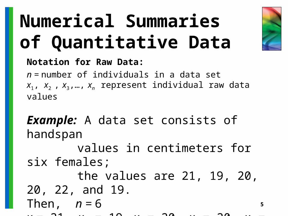
Numerical Summaries of Quantitative Data

Notation for Raw Data:

n = number of individuals in a data setx1, x2 , x3,…, xn represent individual raw data values

Example: A data set consists of handspan values in centimeters for six females; the values are 21, 19, 20, 20, 22, and 19.

Then, n = 6x1= 21, x2 = 19, x3 = 20, x4 = 20, x5 = 22, and x6 = 19

6

Notation and Finding the Quartiles

Split the ordered values into the half that is below the median and the half that is above the median.Q1 = lower quartile

= median of data valuesthat are below the median

Q3 = upper quartile = median of data values

that are above the median

7

Percentiles

The kth percentile is a number that has k% of the data values at or below it and (100 – k)% of the data values at or above it.

• Lower quartile = 25th percentile• Median = 50th percentile• Upper quartile = 75th percentile

8

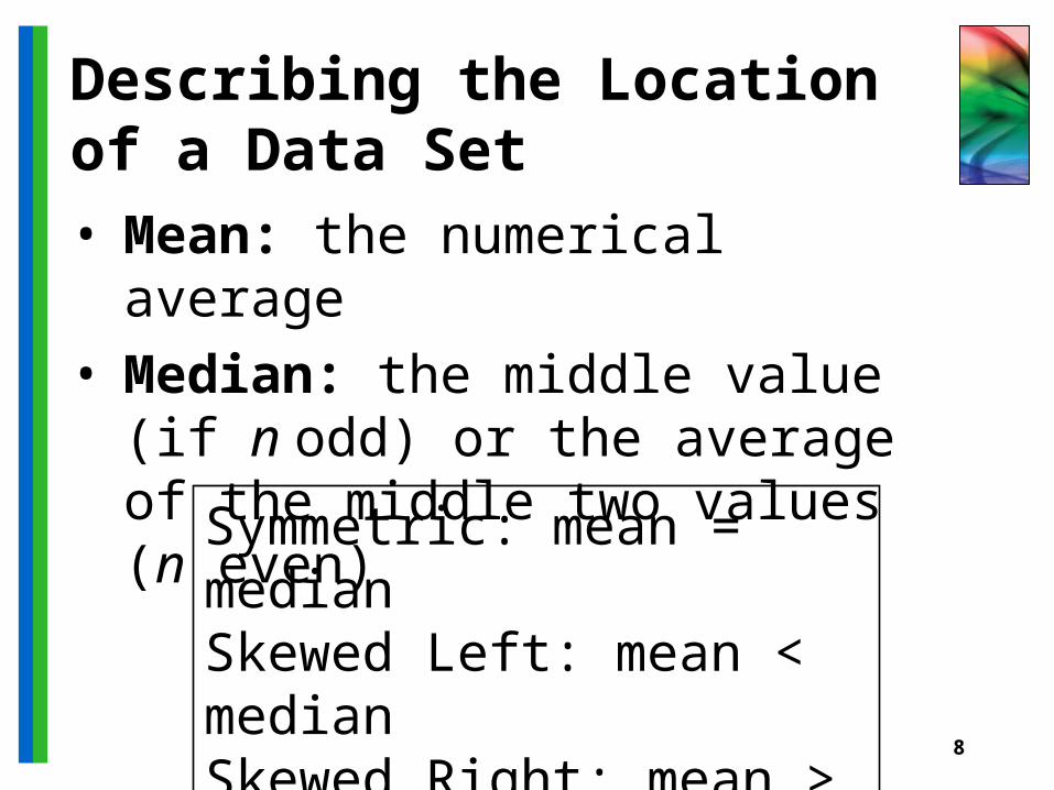
Describing the Location of a Data Set• Mean: the numerical average

• Median: the middle value (if n odd) or the average of the middle two values (n even)

Symmetric: mean = medianSkewed Left: mean < medianSkewed Right: mean > median

9

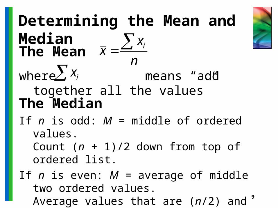
Determining the Mean and Median

The Mean

where means “add together all the values” ixn

xx i

The MedianIf n is odd: M = middle of ordered values.

Count (n + 1)/2 down from top of ordered list.

If n is even: M = average of middle two ordered values.Average values that are (n/2) and (n/2) + 1 down from top of ordered list.

10

Example 2.12 Will “Normal” RainfallGet Rid of Those Odors?

Mean = 18.69 inchesMedian = 16.72 inches

Data: Average rainfall (inches) for Davis, California for 47 years

In 1997-98, a company with odor problem blamed it on excessive rain.That year rainfall was 29.69 inches. More rain occurred in 4 other years.

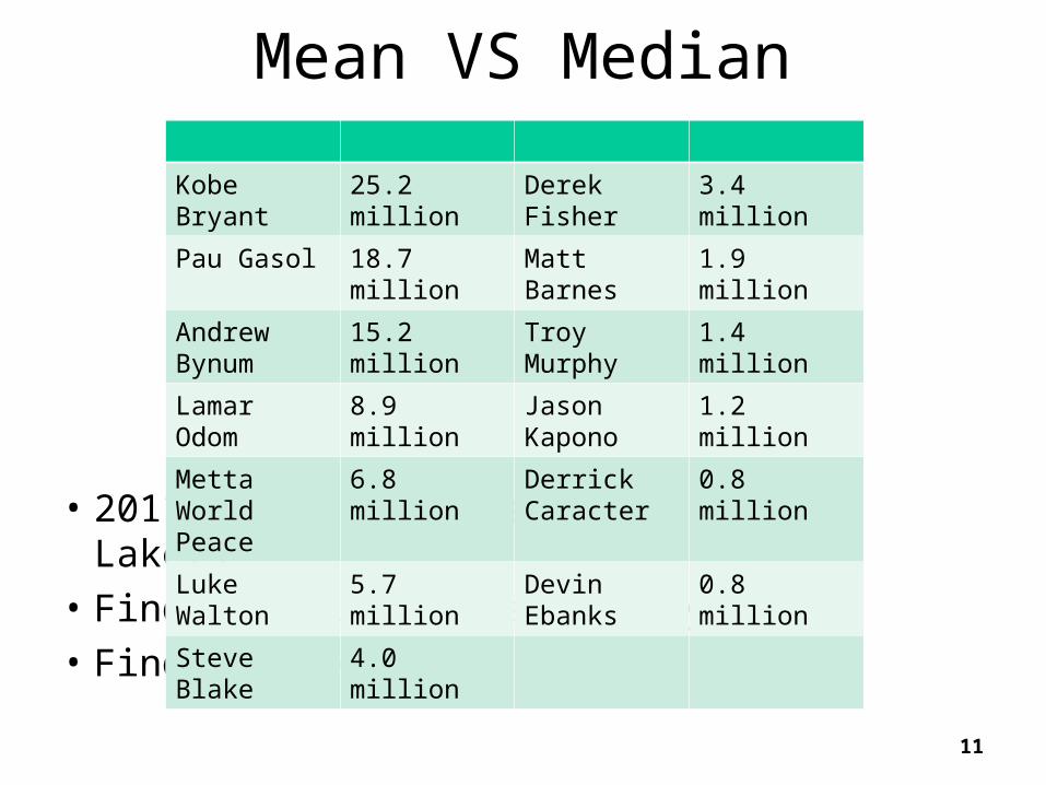
Mean VS Median

• 2011-2012: Salaries of Los Angeles Lakers• Find the five number salary• Find the mean

11

Kobe Bryant 25.2 million Derek Fisher 3.4 million

Pau Gasol 18.7 million Matt Barnes 1.9 million

Andrew Bynum

15.2 million Troy Murphy 1.4 million

Lamar Odom 8.9 million Jason Kapono 1.2 million

Metta World Peace

6.8 million Derrick Caracter

0.8 million

Luke Walton 5.7 million Devin Ebanks 0.8 million

Steve Blake 4.0 million

Choose a Summary

• Skewed Distribution– Use 5 number summary

• Reasonably symmetric distribution – free of outliers– Mean and standard deviation (Since they are

strongly affected by outliers)

12

13

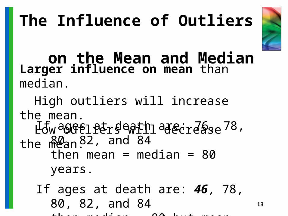
The Influence of Outliers on the Mean and Median

Larger influence on mean than median.

High outliers will increase the mean. Low outliers will decrease the mean.

If ages at death are: 76, 78, 80, 82, and 84then mean = median = 80 years.

If ages at death are: 46, 78, 80, 82, and 84 then median = 80 but mean = 74 years.

14

Describing Spread: Range and Interquartile Range

• Range = high value – low value

• Interquartile Range (IQR) = upper quartile – lower quartile

• Standard Deviation (covered later )

15

Example 2.13 Fastest Speeds Ever Driven

Five-Number Summary for 87 males

• Median = 110 mph measures the center of the data• Two extremes describe spread over 100% of data

Range = 150 – 55 = 95 mph• Two quartiles describe spread over middle 50% of data

Interquartile Range = 120 – 95 = 25 mph

16

Outlier: a data point that is not consistent with the bulk of the data.

How to Handle Outliers

• Look for them via graphs.

• Can have big influence on conclusions.

• Can cause complications in some statistical analyses.

• Cannot discard without justification.

17

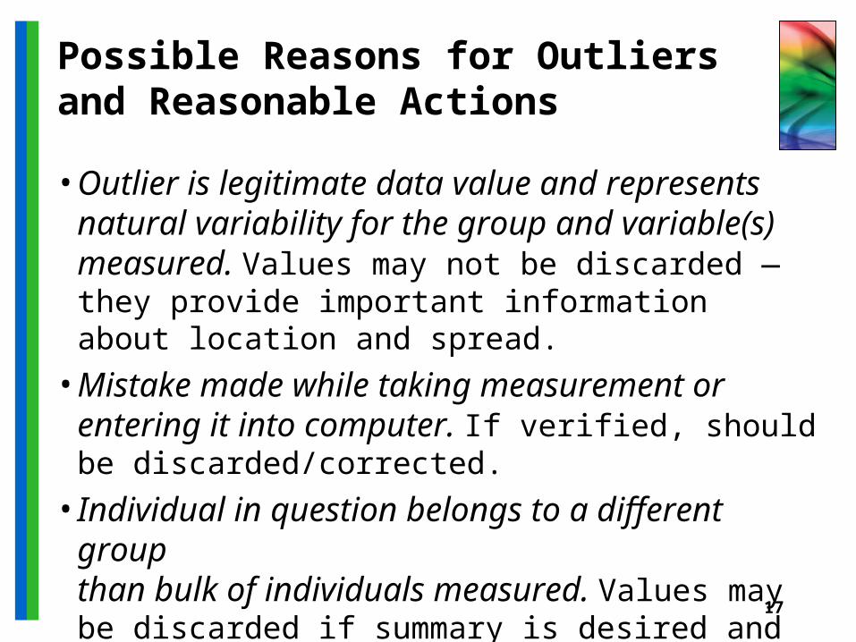
Possible Reasons for Outliersand Reasonable Actions

• Outlier is legitimate data value and represents natural variability for the group and variable(s) measured. Values may not be discarded — they provide important information about location and spread.

• Mistake made while taking measurement or entering it into computer. If verified, should be discarded/corrected.

• Individual in question belongs to a different group than bulk of individuals measured. Values may be discarded if summary is desired and reported for the majority group only.

18

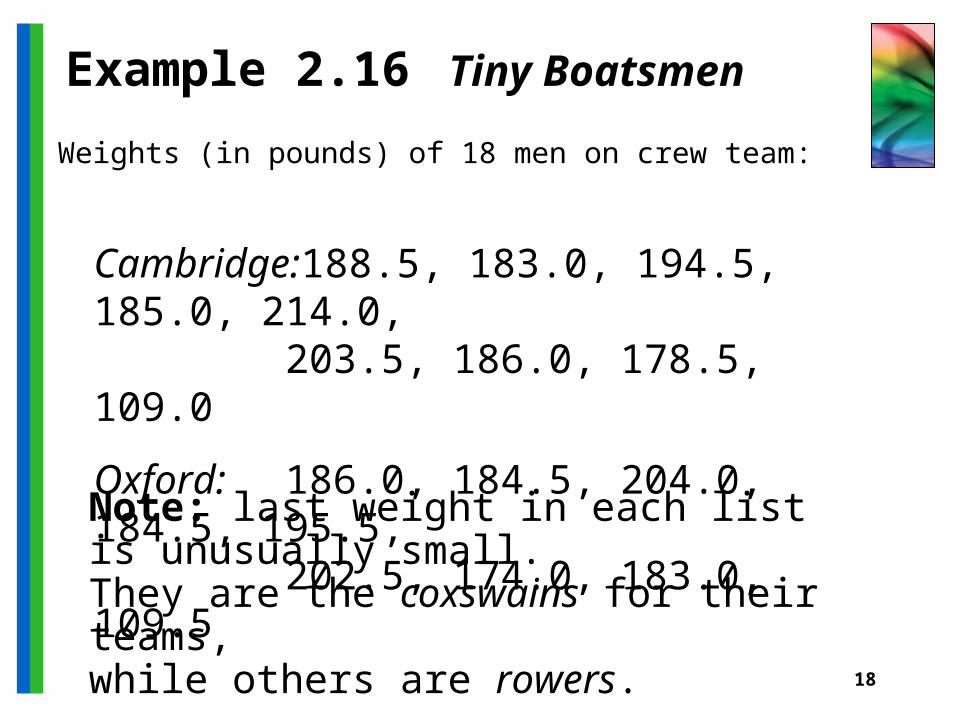
Example 2.16 Tiny Boatsmen

Weights (in pounds) of 18 men on crew team:

Note: last weight in each list is unusually small.

They are the coxswains for their teams, while others are rowers.

Cambridge:188.5, 183.0, 194.5, 185.0, 214.0, 203.5, 186.0, 178.5, 109.0

Oxford: 186.0, 184.5, 204.0, 184.5, 195.5, 202.5, 174.0, 183.0, 109.5

Homework

• Assignment:

•  Chapter 2 – Exercise 2.43 and 2.44

• Chapter 2 – Exercise 2.74 and 2.81

• Reading:

• Chapter 2 – p. 37-46

19