www.elsevier.com/locate/enbuild

Energy and Buildings 39 (2007) 962–974

Numerical study on thermal behavior of classical or

composite Trombe solar walls

Jibao Shen a,b, Stephane Lassue a,*, Laurent Zalewski a, Dezhong Huang b

a Laboratoire d’Artois de Mecanique Thermique et Instrumentation (LAMTI), Faculte des Sciences Appliquees, Universite d’Artois, 62400 Bethune, Franceb Department of Civil Engineering, School of Engineering, Shaoxing College of Arts and Sciences, Shaoxing University, Shaoxing, Zhejiang 312000, China

Received 21 October 2005; received in revised form 20 November 2006; accepted 21 November 2006

Abstract

It is very difficult to calculate and analyze with precision the thermal behavior of the walls of building envelope when coexist various modes of

thermal transfer and because of the particularly random climatic phenomena. These problems are very complex in the case of special components

such as passive solar wall used in ‘‘bio-climatic’’ architecture. In this paper, the thermal performances of passive solar systems, a classical Trombe

wall and a composite Trombe–Michel wall, are studied. The models were developed by our cares with the finite differences method (FDM) [L.

Zalewski, S. Lassue, B. Duthoit, M. Butez, Study of solar walls—validating a numerical simulation model, International Review on Building and

Environment, 37 (1) (2002) 109–121], and with TRNSYS software [Solar Laboratory of energy (USA), Manuals of TRNSYS, University of

Wisconsin-Madison, USA, 1994]. The model for a composite wall developed with FDM was validated by experimentation [1]. The comparisons

between the results of simulation with TRNSYS [2] and with FDM, and between the results of simulation a classical Trombe wall and the results of

simulation and a composite Trombe wall have been made. They show that the models developed by ourselves are very precise, and the composite

wall has better energetic performances than the classical wall in cold and/or cloudy weather.

# 2006 Elsevier B.V. All rights reserved.

Keywords: Passive solar system; Solar wall; Classical wall; Composite wall; Finite difference method; TRNSYS

1. Introduction

The passive solar walls collect and store solar energy which

can contribute to the heating of buildings. Most known is the

classical Trombe wall, passive solar system. A glazing is

installed at a small distance from a massive wall. The wall

absorbs solar radiation and transmits parts of it into the interior of

the building by natural convection through a solar chimney

formed by the glazing on one side and the wall on the other. The

principal advantage of the classical Trombe wall is its simplicity,

but one major problem is its small thermal resistance. If the solar

energy received by the wall is reduced, during the night or

prolonged cloudy periods, some heat flux is transferred from the

* Corresponding authors at: Laboratoire d’Artois de Mecanique Thermique et

Instrumentation (LAMTI), Faculte des Sciences Appliquees, Universite

d’Artois, 62400 Bethune, France. Tel.: +33 3 21 63 71 54;

fax: +33 3 21 63 71 23.

E-mail addresses: articlejbs2004@yahoo.com.cn (J. Shen),

lassue@univ-artois.fr (S. Lassue), laurent.zalewski@univ-artois.fr

(L. Zalewski).

0378-7788/$ – see front matter # 2006 Elsevier B.V. All rights reserved.

doi:10.1016/j.enbuild.2006.11.003

inside to the outside, which results in excessive heat loss from the

building. This problem becomes important in the regions with

cold climates and/or with high latitudes. A solution is to use a

composite Trombe–Michel wall [7] which includes an insulating

layer. Zrikem and Bilgen [3], Zalewski [4].

It is rather difficult to establish a general rule to calculate

with precision the capacity of storage and of energy

recuperation of solar energy for this sort of wall. It is necessary

for that to resort to simulation tools such as TRNSYS developed

by the members of US Solar Energy Laboratory at the

University of Wisconsin-Madison. Thanks to the component

Type 36 of TRNSYS, we can easily study the classical Trombe

wall. To study the composite Trombe–Michel wall, we

designed a new simulation component.

In this work, the classical and composite wall systems are

studied and the finite differences method is used. In the

following section, the thermal study of a classical wall and a

composite wall, the comparisons of the simulation results by

TRNSYS and those of simulation with the finite difference

method (FDM) are presented. The comparisons between both

walls are also presented.

Nomenclature

a thermal diffusivity (m2/s)

A area (m2)

C specific heat (J/kg 8C)

Cd discharge coefficient

D distance (m)

g acceleration of gravity (m/s2)

Gr Grashof number

he convection coefficient (W/m2 8C)

hr radiation coefficient (W/m2 8C)

H height (m)

Ho vertical distance between two vents (m)

Ig global solar radiation flux density (W/m2)

Id diffuse solar radiation flux density (W/m2)

Ih solar radiation flux density on a horizontal

surface (W/m2)

L width (m)

m air mass flow rate (kg/s)

Nu Nusselt number

Pr Prandtl number

Q thermal energy (J)

Ra Rayleigh number

t time (s)

T temperature (8C)

Tabs temperature (K)

V fluid velocity (m/s)

x, z Cartesian coordinates

X thickness (m)

Greek letters

a solar absorptivity

b thermal expansion coefficient (K�1)

e emissivity

z sum of load loss coefficients

l thermal conductivity (W/m 8C)

m dynamic viscosity (kg/m s)

r density (kg/m3)

s Stefan–Boltzmann constant (5.674 � 10�8 W/

m2 K4)

t transmissivity

w heat flux density (W/m2)

F heat flux (kJ/h)

Subscripts

abs absolute temperature

am ambiance

c convection

e emission

e exterior

env environment

f fluid

g glazing

gy gypsum

i insulating

int interior (dwelling)

m massive wall

o orifice of ventilation (vent)

r radiation

s solar

sf surface

J. Shen et al. / Energy and Buildings 39 (2007) 962–974 963

In this work, the meteorological data used are the one

from Carpentras in south of France (latitude 44.058N,

longitude 5.038E). The parameters of the composite wall are

based on a previous experimental study Zalewki and

coworkers [4,5]. To compare both walls, some parameters

of the classical wall are based on that of the experimental

composite wall. With the component Type 36 of TRNSYS,

we consider only one layer for the massive wall (the layer of

gypsum is not considered for simulations of the classical

wall). It will be assumed that the thermal exchange exists in

only one direction only and there are no heat losses in the

others.

2. Classical Trombe wall

2.1. Functioning principle

The classical Trombe wall is constituted of a massive

wall installed at a small distance from a glazing. In the case

of the thermo-circulation phenomenon, the massive wall

absorbs the solar flux through the glazing(s). The wall

transfers a part of the flux inside the building by conduction.

The heating of the air in contact with this wall induces a

natural circulation: the air is admitted by the lower vent of

the wall and comes back to the room by the upper vent. The

air circulating, transfers part of the solar heat flux (cf. left

part of Fig. 1).

An inverse thermo-siphon phenomenon was observed at the

time of little or non-sunny periods at night or in winter. In fact,

when the wall becomes colder than the indoor temperature, an

air circulation, from the vent on top to the vent at the bottom,

produces itself and comes to cool the habitat. To resolve this

problem, we can, for example, place a supple plastic film at the

level of the orifices, when there is a thermo-siphon

phenomenon. The vents are then opened, and in the opposite

case they are closed.

Fig. 1. Classical Trombe wall.

J. Shen et al. / Energy and Buildings 39 (2007) 962–974964

2.2. Description of the classical Trombe wall for studying

We choose to compare the results of TRNSYS simulation

with those of simulation by FDM. The parameters of the wall

based on a previous experimental study of the composite wall

Zalewski [4]. The geometric characteristics of the classical

Trombe wall studied are illustrated in Fig. 1.

The wall studied has the following characteristics:

(1) A

zimuth surface angle of the wall, g = 0 (South

orientation).

(2) W

all height, H = 2.47 m.

(3) W

all width, L = 1.34 m.

(4) M

assive wall thickness, X = 0.15 m.

(5) M

assive wall conductivity, lm = 0.8117 W/(m 8C).

(6) T

hermal capacity of the massive wall, rmCm = 1.803

� 106 J/(m3 8C) (rm = 1900 kg/m3, Cm = 949 J/kg 8C).

(7) S

olar absorption of the massive wall, a = 0.9.

Fig. 2. Analogical diagram of classical Trombe wall.

(8) E missivity of the massive wall, em = 0.9.

(9) E

missivity of the glazing, eg = 0.9.

(10) N

umber of glazing, Ng = 1.

(11) D

istance between the surface of the glazing and one of the

massive wall, D = 0.03 m.

(12) S

urface of the massive wall vent, Ao = 0.15 � 0.60

= 0.09 m2.

(13) V

ertical distance between two vents, Ho = 2.15 m.

(14) T

emperature of the dwelling, Tint = 19 8C (constant).

(15) G

lobal exchange coefficient (by convection and by

radiation) between the surface of the massive wall and

the dwelling, hint = hr int + hc int = 9.1 W/(m2 8C).

(16) T

ransmissivity of the glazing, t = 0.81.

2.3. Analysis of the different thermal exchanges

The analysis of the different thermal exchanges for the

classical wall is similar to that for the composite wall presented

in the next section. The analogical diagram of the thermal heat

transfer in the classical wall is shown in Fig. 2.

The Type 36 of TRNSYS uses only one parameter for the

height of the wall and the distance between two vents, and one

layer for the massive wall. Since the air mass flow rate in the

chimney formed by the glazing and the massive wall flows

between two openings of ventilation, we only considered the

wall surface between these two vents (H = 2.15 m,

L = 1.34 m).

3. Composite Trombe–Michel wall

3.1. Functioning principle

The functioning of a composite Trombe–Michel wall is

similar to that of a classical Trombe wall. But the latter induces

important heat loss during the cold periods due to the small

thermal resistance of the massive wall. We can remedy this

problem while using the composite wall. The latter has an

insulating wall at the back of the massive wall. The thermal

energy can be transferred from outside to the interior air layer

by conduction in the massive wall. Then it can be transferred by

convection while using the thermo-circulation phenomenon of

air between the massive wall and the insulating wall. At the

time of little or non-sunny days during winter or at nights, the

vents in the insulating wall are closed. Thanks to the big

thermal resistance, there is little thermal flux that going from

indoor to outdoor (little loss) (cf. Fig. 3).

This passive solar wall has been studied experimentally

within the framework of Zalewski’s [4]. The measurements

were realized on the Cadarache site in the south of France and

made possible to set up a simulation model based on the use of

the finite difference method FDM.

Simultaneous measurements of heat fluxes and of surface

temperatures particularly at the level of the massive wall have

allowed us to quantify the energetic performances of this

component and to validate our simulation model within the

framework of an experimental follow up which lasted several

years.

For example one can observe the good correspondence

between the heat flows measured and simulated in Fig. 4, here

during a week in winter.

This model made possible to position the composite Trombe

wall as regards the more classical walls in terms of energetic

balance for heating period (1/10 to 20/05, see Fig. 5).

3.2. Description of the composite Trombe–Michel wall for

studying

We chose the parameters of the composite Trombe–Michel

wall according to the previous experimental study Zalewski and

coworkers [4,5]. The geometric characteristics of the wall

studied are illustrated by Fig. 3.

The wall exposed to the south has the following

characteristics:

(1) W

all height, H = 2.47 m.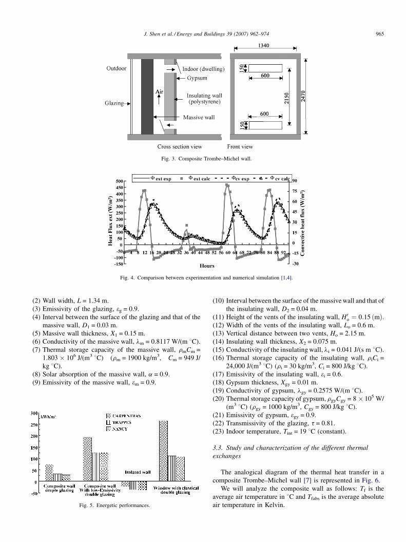

Fig. 3. Composite Trombe–Michel wall.

Fig. 4. Comparison between experimentation and numerical simulation [1,4].

J. Shen et al. / Energy and Buildings 39 (2007) 962–974 965

(2) W

all width, L = 1.34 m.

(3) E

missivity of the glazing, eg = 0.9.

(4) I

nterval between the surface of the glazing and that of the

massive wall, D1 = 0.03 m.

(5) M

assive wall thickness, X1 = 0.15 m.

(6) C

onductivity of the massive wall, lm = 0.8117 W/(m 8C).

(7) T

hermal storage capacity of the massive wall, rmCm =

1.803 � 106 J/(m3 8C) (rm = 1900 kg/m3, Cm = 949 J/

kg 8C).

(8) S

olar absorption of the massive wall, a = 0.9.

(9) E

missivity of the massive wall, em = 0.9.

Fig. 5. Energetic performances.

(10) I

nterval between the surface of the massive wall and that of

the insulating wall, D2 = 0.04 m.

(11) H

eight of the vents of the insulating wall, H0o ¼ 0:15 ðmÞ. (12) W idth of the vents of the insulating wall, Lo = 0.6 m.

(13) V

ertical distance between two vents, Ho = 2.15 m.

(14) I

nsulating wall thickness, X2 = 0.075 m.

(15) C

onductivity of the insulating wall, li = 0.041 J/(s m 8C).

(16) T

hermal storage capacity of the insulating wall, riCi =

24,000 J/(m3 8C) (ri = 30 kg/m3, Ci = 800 J/kg 8C).

(17) E

missivity of the insulating wall, ei = 0.6.

(18) G

ypsum thickness, Xgy = 0.01 m.

(19) C

onductivity of gypsum, lgy = 0.2575 W/(m 8C).

(20) T

hermal storage capacity of gypsum, rgyCgy = 8 � 105 W/

(m3 8C) (rgy = 1000 kg/m3, Cgy = 800 J/kg 8C).

(21) E

missivity of gypsum, egy = 0.9.

(22) T

ransmissivity of the glazing, t = 0.81.

(23) I

ndoor temperature, Tint = 19 8C (constant).

3.3. Study and characterization of the different thermal

exchanges

The analogical diagram of the thermal heat transfer in a

composite Trombe–Michel wall [7] is represented in Fig. 6.

We will analyze the composite wall as follows: Tf is the

average air temperature in 8C and Tfabs is the average absolute

air temperature in Kelvin.

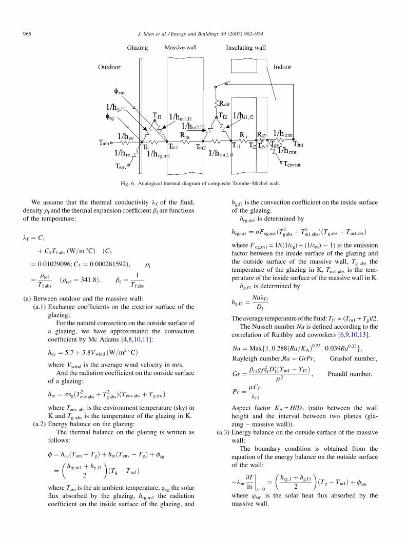
Fig. 6. Analogical thermal diagram of composite Trombe–Michel wall.

J. Shen et al. / Energy and Buildings 39 (2007) 962–974966

We assume that the thermal conductivity lf of the fluid,

density rf and the thermal expansion coefficient bf are functions

of the temperature:

lf ¼ C1

þ C2T f abs ðW=m �CÞ ðC1

¼ 0:01029096; C2 ¼ 0:000281592Þ; rf

¼ rref

T f abs

ðrref ¼ 341:8Þ; bf ¼1

T f abs

(a) B

etween outdoor and the massive wall:

(a.1) Exchange coefficients on the exterior surface of the

glazing;

For the natural convection on the outside surface of

a glazing, we have approximated the convection

coefficient by Mc Adams [4,8,10,11]:

hce ¼ 5:7þ 3:8Vwind ðW=m2 �CÞ

where Vwind is the average wind velocity in m/s.

And the radiation coefficient on the outside surface

of a glazing:

hre ¼ segðT2env abs þ T2

g absÞðTenv abs þ Tg absÞ

where Tenv abs is the environment temperature (sky) in

K and Tg abs is the temperature of the glazing in K.

(a.2) Energy balance on the glazing:

The thermal balance on the glazing is written as

follows:

f ¼ hceðTam � TgÞ þ hreðTenv � TgÞ þ fsg

¼�

hrg;m1 þ hg;f1

2

�ðTg � Tm1Þ

where Tam is the air ambient temperature, wsg the solar

flux absorbed by the glazing, hrg,m1 the radiation

coefficient on the inside surface of the glazing, and

hg,f1 is the convection coefficient on the inside surface

of the glazing.

hrg,m1 is determined by

hrg;m1 ¼ sFeg;m1ðT2g abs þ T2

m1 absÞðTg abs þ Tm1 absÞ

where Feg,m1 = 1/((1/eg) + (1/em) � 1) is the emission

factor between the inside surface of the glazing and

the outside surface of the massive wall, Tg abs the

temperature of the glazing in K, Tm1 abs is the tem-

perature of the inside surface of the massive wall in K.

hg,f1 is determined by

hg;f1 ¼Nulf1

D1

The average temperature of thefluid:Tf1 = (Tm1 + Tg)/2.

The Nusselt number Nu is defined according to the

correlation of Raithby and coworkers [6,9,10,13]:

Nu ¼ Maxf1; 0:288ðRa=KAÞ0:25; 0:039Ra0:33g;Rayleigh number;Ra ¼ GrPr; Grashof number;

Gr ¼ bf1gr2f1D3

1ðTm1 � T f1Þm2

; Prandtl number;

Pr ¼ mCf1

lf1

Aspect factor KA = H/D1 (ratio between the wall

height and the interval between two planes (gla-

zing � massive wall)).

(a.3) Energy balance on the outside surface of the massive

wall:

The boundary condition is obtained from the

equation of the energy balance on the outside surface

of the wall:

�lm

@T

@x

����x¼0

¼�

hrg;1 þ hg;f1

2

�ðTg � Tm1Þ þ fsm

where wsm is the solar heat flux absorbed by the

massive wall.

J. Shen et al. / Energy and Buildings 39 (2007) 962–974 967

(b) I

n the massive wall (conduction):

The thermal flux through the massive wall is determined

by the one-dimensional equation:

@T

@t¼ am

@2T

@x2ð0< x<X1Þ

am is the diffusivity of the massive wall, am = lm/rmCpm.

(c) B

etween the massive wall and the insulating wall:

(c.1) Radiation coefficient:

The radiation coefficient between the inside

surface of the massive wall and the outside surface

of the insulating wall:

hrm2;i1 ¼ sFem2;i1ðT2m2 abs þ T2

i1 absÞðTm2 abs þ T i1 absÞ

where Fem2, i1 = 1/((1/em) + (1/ei) � 1) is the emis-

sion factor between the inside surface of the mas-

sive wall and the outside surface of the insulating

wall, Tm2 abs the temperature on the inside surface

of the massive wall in K, and Ti1 abs is the tem-

perature on the outside surface of the insulating

wall in K.

(c.2.) Air mass flow in the chimney—load losses (case of

the open vents).

(c.2.1) Air mass flow rate.

The flow in the chimney is produced

naturally by the thermo-siphon. The thermal

resistance between the inside surface of the

massive wall and the outside surface of the

insulating wall, depends on the air mass flow

through the opening vents in the insulating

wall. In our case this thermal resistance is

calculated on the assumption that all the load

losses are caused by the upper and lower air

vent.

The air mass flow in the chimney is

produced between two vents, so we only

considered the wall section between these

vents (Ho = 2.15 m, L = 1.34 m).

We suppose that the air temperature in the

chimney varies linearly along the chimney

height. The air average temperature in the

space between the inside surface of the

massive wall and the ‘‘outside’’ surface of

the insulating wall will therefore be

T f2 ¼ðTo bottom þ To topÞ

2where To top is the air temperature in the upper

vent and To bottom is the air temperature in the

lower vent.

The air mass flow is directly linked to the

difference of the air temperatures existing

between the vents, and equally to the sum of

the load losses produced during the air flow

crossing the chimney (i.e. Idel’cik [14]).

The global load loss DH, sum of load

losses by friction and the load losses unique,

is equal to

DH ¼ zgf2V2

f2

2g

where z is the sum of the load losses coeffi-

cients, gf2 the average specific weight of the

air in the chimney, and Vf2 is the average

velocity of the air mass flow in the chimney.

While assuming the air to be perfect gas,

admitting the hypothesis of a permanent flow

and following the one-dimensional vertical one

(z), and neglecting the viscosity effects, we

obtain the load loss between the entry (lower

vent) and the exit of the canal (upper vent):

DH ¼Z Ho

0

g dz

where Ho is the vertical distance between the

orifices.

While supposing that the temperature

varies linearly on the journey of the air along

the wall, from the two preceding relations, we

deduce the speed of the air in the chimney:

V f2 ¼ Cd

ffiffiffiffiffiffiffiffiffiffiffiffiffiffiffiffiffiffiffiffiffiffiffiffiffiffiffiffiffiffiffiffiffiffiffiffiffiffiffiffiffiffiffiffiffiffiffiffiffiffiffiffiffigHoðTo top abs � To bottom absÞ

To top abs þ To bottom abs

s

where Cd ¼ffiffiffiffiffiffiffi2=z

pis the discharge coeffi-

cient, To top abs the air temperature at the upper

vent in K, and To bottom abs is the air tempera-

ture at the lower vent in K.

The sum of the load loss coefficients is

determined by

z ¼ zlinear þ zentry

rf2

rfl

�Achim

Ao

�2

þ zout

rf2

rfo

�Achim

Ao

�2

þ zo bottom

rf2

rfl

�Achim

Ao

�2

þ zo top

rf2

rfo

�Achim

Ao

�2

þ zelbow :bottom

rf2

rfl

�Achim

Ao

�2

þ zelbow top

where Achim/Ao is the ratio between the chim-

ney section and that of the orifices, rf2 the

density at the average temperature Tf2, rfl the

density at the average temperature To bottom, rfo

the density at the average temperature To top,

zlinear the linear load loss in the chimney, zentry

the load singular loss coefficient at the entry,

zout the load loss coefficient at the exit (rush

expansion), zo the load loss coefficient at the

level of the orifices (zo bottom and zo top), and

J. Shen et al. / Energy and Buildings 39 (2007) 962–974968

zelbow is the load loss coefficient at the level of

the elbows (zelbow bottom and zelbow top).

Here, the coefficients zelbow depends on the

dimensions of the chimney, its orifice, on the

angle of the elbows, and also on the nature of

the materials. If the device contains a ‘‘dead’’

zone in the ventilated air layer upon the upper

vent, the coefficient zelbow must be increased

by 20% [14].

It is therefore possible to calculate the air

mass flow rate m in the chimney as follows:

m

rf2

¼ CdA

ffiffiffiffiffiffiffiffiffiffiffiffiffiffiffiffiffiffiffiffiffiffiffiffiffiffiffiffiffiffiffiffiffiffiffiffiffigHoðTo abs � T i absÞ

To abs þ T i abs

s

Then the air mass flow is calculated by the

following formula:

m ¼ rf2CdA

ffiffiffiffiffiffiffiffiffiffiffiffiffiffiffiffiffiffiffiffiffiffiffiffiffiffiffiffiffiffiffiffiffiffiffiffiffiffiffiffiffiffiffiffiffiffiffiffiffiffiffiffiffigHoðTo top abs � To bottom absÞ

To top abs þ To bottom abs

s

(c.2.2) Thermal balance in the chimney (convection)

The thermo-circulation is produced when

the average temperature in the chimney is

higher than that of the indoor temperature.

The thermal energy transported by the air

towards the top orifice is written as

fo ¼mCf2ðTo top � To bottomÞ

Am

¼ hm2;f2ðTm2 � T f2Þ þ hi1;f2ðT i1 � T f2Þ

where hm2,f2 is the convection coefficient at

the inside surface of the massive wall and

hi1,f2 is the convection coefficient at the out-

side surface of the insulating wall.

hm2,f2, hi1,f2 are determined by

hm2;f2 ¼ hi1;f2 ¼Nulf2

Ho

The Nusselt number is defined according to

the correlation of Fishenden and Saunders

[3,15]:

Nu ¼ 0:107Gr1=3

The Grashof number is defined as follows:

Gr ¼ bf2gr2f2H3

oðTo top � To bottomÞm2

(c.2.3) Energy balance on the inside surface of the

massive wall:

The boundary condition is obtained from

the equation of the energy balance on the

inside surface of the wall:

�lm

@T

@X

����x¼x1

¼ hm2;f2ðTm2 � T f2Þ þ hrm2;i1ðTm2 � T i1Þ

(c.2.4) Energy balance on the outside surface of the

insulating wall:

The boundary condition is obtained from

the equation of the energy balance on the

outside surface of the insulating wall:

�li

@T

@X

����x¼0

¼ hi1;f2ðT f2 � Tm2Þ þ hrm2;i1ðTm2 � T i1Þ

(c.3) Case in which the vents are closed:

(c.3.1) Energy balance on the inside surface of the

massive wall:

The boundary condition is obtained from

the equation of the energy balance on the

inside surface of the wall:

�lm

@T

@X

����x¼x1

¼ ðhm2;i1 þ hrm2;i1ÞðTm2 � T i1Þ

(c.3.2) Energy balance on the outside surface of the

insulating wall:

The boundary condition is obtained from

the equation of the energy balance on the

outside surface of the insulating wall:

�li

@T

@X

����x¼0

¼ ðhm2;i1 þ hrm2;i1ÞðTm2 � T i1Þ

(c.3.3) Convection coefficient:

hm2;i1 ¼hm2;f2

2¼ hi1;f2

2

hm2,f2 is determined by

hm2;f2 �Nulf2

D2

The Nusselt number Nu is defined according

to the correlation of Raithby and coworkers

[6,9,10,13]:

Nu¼Maxf1;0:288ðRa=KAÞ0:25; 0:039Ra0:33g;Rayleigh number;Ra¼GrPr;

Grashof number;Gr ¼ bf2gr2f2D3

2ðTm2� T f2Þm2

;

Prandtl number;Pr ¼ mCf2

lf2

KA = H/D2 is the ratio between the wall height

and the two planes’ interval.

(d) In the insulating wall (heat conduction):

The thermal flux through the insulating wall is

determined by the one-dimensional equation:

@T

@t¼ ai

@2T

@X2ð0<X<X2Þ

ai is the diffusivity of the insulating wall, ai = li/riCpi.

(e) On the interface between the insulating wall and

gypsum:

Fig. 7. Meteorological data: solar horizontal heat flux, Ih; solar diffuse heat flux, Id.

J. Shen et al. / Energy and Buildings 39 (2007) 962–974 969

The thermal flux is determined by the equation:

@T

@t¼ ai gy

@2T

@X2ð�dx<X< dxÞ

ai gy is the average diffusivity of the insulation mate-

rial and the gypsum and dx is a small element.

(f) On the inner surface of the insulating wall (on the

surface of the gypsum):

The boundary condition is obtained from the

equation of energy balance on the inside surface of

the wall:

�lgy

@T

@X

����x¼x2

¼ hintðTgy2 � T intÞ

with hint = hr gy2 + hc gy2.

The radiation coefficient on the inside surface of the

insulating wall towards the heated room:

hr gy2 ¼ segy2ðT2gy2 abs þ T2

int absÞðTgy2 abs þ T int absÞ

The convection coefficient on the inside surface of the insulat-

ing wall:

Hc gy2 ¼Nulf2

Hi

where Hi is the insulating wall height.

For the calculation of the coefficient hc gy2, we use the

correlations proposed by the ASHRAE in natural convection

Fig. 8. Meteorological data: outdoor air temp

for vertical plates [12,16]:

if 104 <GrH < 108; NuH

¼ 0:516Ra1=4H ; if 108 <GrH < 1012; NuH

¼ 0:117Ra1=3H ; Rayleigh number;RaH

¼ GrHPr; Grashof number;GrH

¼ bfigr2fiH

3i ðTgy2 � T intÞm2

; Prandtl number;Pr ¼ mCf int

lf int

4. Meteorological data

We have carried out the simulations of the classical Trombe

wall and the composite Trombe–Michel wall for 10 days (from

the 57th to the 66th day, i.e. from February 26 to March 7). The

meteorological data are shown in Figs. 7 and 8. During the first

day, there was a lot of sunlight, the horizontal solar flux Ih is big.

After 3 days, there were a lot of clouds, the temperature of the

air Tam went down, and the velocity of the wind Vwind raised.

During the last day of this period, there was a lot of sun, the

horizontal solar flux Ih raised.

5. Comparison of the results of simulations with

TRNSYS and FDM

We carried out the simulations of the solar walls with

TRNSYS and with the finite differences method (FDM). The

erature, Tam; velocity of the wind, Vwind.

Fig. 9. Comparison of the temperature Tsf outside on the outside surface of the massive wall in the classical wall.

J. Shen et al. / Energy and Buildings 39 (2007) 962–974970

model with FDM had been validated in comparison

with experimental results in the case of the composite wall

and then modified in order to simulate the functioning of

the classical wall Zalewski [4]. In this section, we will

compare the simulation results of both methods. It means that

we consider the wall without insulation and with air

circulation through the massive concrete wall (classical

Trombe wall).

5.1. Comparison on the classical wall

Figs. 9–11 indicate the temperature Tsf outside on the outside

surface of the massive wall, the temperature Tsf inside on the

inside surface of the massive wall and the temperature To of the

air in the upper vent in the classical wall.

Figs. 12 and 13 indicate the thermal flux Fo transferred from

the ventilated air layer to the dwelling and the thermal flux

Fsf inside transferred from the inside surface of the massive wall

to the dwelling in the classical wall.

In the simulations with TRNSYS, the Type 36 uses the

constant global coefficient hint. In reality, hint increases with the

temperature difference between the surface and the fluid.

Therefore, the temperatures Tsf inside obtained by the two

methods are different (see Fig. 10). On the other hand, Tsf inside

is a little lower when hint increases. The heat flux Fsf inside is

almost the same (see Fig. 13).

The discharge coefficient Cd is constant in the simulations

with TRNSYS. The discharge coefficient Cd is determined by

Fig. 10. Comparison of the temperature Tsf inside on the in

the equation:

Cd ¼ffiffiffi2

z

s

where z is the sum of the load loss coefficients:

z ¼ C1

�Achim

Ao

�2

þ C2 ðC1 ¼ 8;C2 ¼ 4Þ

where Achim/Ao is the ratio of the chimney area to that of the

orifices, representing the load loss. The discharge coefficient Cd

is supposed to be constant.

Contradictory, the discharge coefficient is not constant. It

changes with the air speed in the chimney Vf. When the solar

heat flux Ih increases, the temperature Tsf outside on the outside

surface of the wall increases with it. And when the speed Vf

increases, the discharge coefficient Cd increases. Therefore, the

heat flux Fo increases. In the simulations with TRNSYS, since

Cd is constant, the amplitudes of Fo are smaller (see Fig. 12).

5.2. Comparison on the composite wall

Figs. 14–16 indicate the temperature Tsf outside of the outside

surface of the massive wall, the temperature Tsf inside of the

inside surface of the insulating wall and the temperature To of

the air in the wall top orifice in the composite wall.

side surface of the massive wall in the classical wall.

Fig. 11. Comparison of the temperature To of the air at the upper vent in the classical wall.

Fig. 12. Comparison of the thermal flux Fo in the classical wall.

J. Shen et al. / Energy and Buildings 39 (2007) 962–974 971

Fig. 17 indicates the thermal flux Fo from the ventilated air

layer to the dwelling in the composite Trombe wall.

To calculate the solar flux with TRNSYS, we used the Type

16 (Solar Radiation Processor) TRNSYS manual [2]. But with

FDM, we used another method describe by [13,14].

Because of the different calculations, the global solar flux on

the vertical wall in the simulation with FDM is a little bigger than

that in the simulation with TRNSYS. We can notice that the

results in the simulation with FDM are a little bigger than that in

the simulation with TRNSYS. Figs. 14–17 shows that the results

of the two methods are again very similar. The simulations with

TRNSYS for the composite wall seem successful.

Fig. 13. Comparison of the thermal fl

6. Comparison between the two walls

We will make comparisons between the two types of walls

(see Figs. 18–22).

According to the figures, we note that, every day, the

amplitudes of the values for the composite wall are smaller than

those for the classical wall.

For the classical wall, at the time of day when it is not very

sunny, the minimum Tsf inside is inferior to Tint by 2 8C while on

sunny day, the maximum Tsf inside is more than 26 8C. For the

composite wall, the difference between Tsf inside and Tint is less

than 1 8C.

ux Fsf inside in the classical wall.

Fig. 14. Comparison of the temperatures Tsf outside on the outside surface of the massive wall in the composite wall.

Fig. 15. Comparison of the temperatures Tsf inside on the inside surface of the insulating wall in the composite wall.

Fig. 16. Comparison of the temperatures To of the air at the upper vent in the composite Trombe wall.

Fig. 17. Comparison of the thermal flux Fo in the composite wall.

J. Shen et al. / Energy and Buildings 39 (2007) 962–974972

Fig. 18. Comparison of the temperatures Tsf outside of the outside surface of the massive wall.

Fig. 19. Comparison of the temperature Tsf inside on the inside surface of the wall.

J. Shen et al. / Energy and Buildings 39 (2007) 962–974 973

For the heating by solar walls, the thermal flux Fo from the

ventilated air layer to the dwelling and the thermal flux Fsf inside

from the inside surface of internal wall to the heating room are

the most important parameters. Therefore, we are going to

study these parameters.

Since the solar flux enter directly into the chimney between

the glazing and the massive wall of the classical wall, the

temperature of the fluid between the glazing and the massive

wall is directly influenced by the solar thermal radiation. And

the thermal flow that is lost crosses directly the glazing towards

the exterior. The amplitudes of the air mass flow, of the

temperature To of the air in the upper vent and of the thermal

flux Fo from the air layer to the dwelling are therefore bigger.

With the composite wall, the solar flux is absorbed by the

massive wall, and then some of it crosses the massive wall, and

finally enters the chimney between the massive wall and the

Fig. 20. Comparison of the temperatures To

insulating wall. The entering or lost flux crosses the massive

wall. The massive wall, with its great heat capacity, induced a

dephasing on the heat fluxes evolution. The amplitudes of the

air mass flow, of the temperature To of the air at the top orifice

and of the thermal flux Fo from the orifice to the room are then

smaller. And the changes of the amplitudes are delayed. On

sunny days, the thermal flux enters the dwelling continually at

night by the air mass flow. On sunny days and during the first

day when it is not very sunny (60th day), it heats again the room

at night. But the classical wall cannot heat the room at the

night.

Since the thermal resistance of the insulating wall is bigger

than that of the massive wall, the amplitudes of the temperature

of the inside surface of the internal wall Tsf inside and of the flux

from the inside surface of internal wall to the room Fsf inside are

smaller in the composite wall.

of the air at the upper vent of the wall.

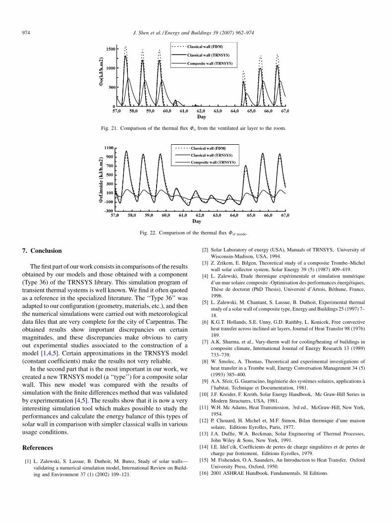
Fig. 21. Comparison of the thermal flux Fo from the ventilated air layer to the room.

Fig. 22. Comparison of the thermal flux Fsf inside.

J. Shen et al. / Energy and Buildings 39 (2007) 962–974974

7. Conclusion

The first part of our work consists in comparisons of the results

obtained by our models and those obtained with a component

(Type 36) of the TRNSYS library. This simulation program of

transient thermal systems is well known. We find it often quoted

as a reference in the specialized literature. The ‘‘Type 36’’ was

adapted to our configuration (geometry, materials, etc.), and then

the numerical simulations were carried out with meteorological

data files that are very complete for the city of Carpentras. The

obtained results show important discrepancies on certain

magnitudes, and these discrepancies make obvious to carry

out experimental studies associated to the construction of a

model [1,4,5]. Certain approximations in the TRNSYS model

(constant coefficients) make the results not very reliable.

In the second part that is the most important in our work, we

created a new TRNSYS model (a ‘‘type’’) for a composite solar

wall. This new model was compared with the results of

simulation with the finite differences method that was validated

by experimentation [4,5]. The results show that it is now a very

interesting simulation tool which makes possible to study the

performances and calculate the energy balance of this types of

solar wall in comparison with simpler classical walls in various

usage conditions.

References

[1] L. Zalewski, S. Lassue, B. Duthoit, M. Butez, Study of solar walls—

validating a numerical simulation model, International Review on Build-

ing and Environment 37 (1) (2002) 109–121.

[2] Solar Laboratory of energy (USA), Manuals of TRNSYS, University of

Wisconsin-Madison, USA, 1994.

[3] Z. Zrikem, E. Bilgen, Theoretical study of a composite Trombe–Michel

wall solar collector system, Solar Energy 39 (5) (1987) 409–419.

[4] L. Zalewski, Etude thermique experimentale et simulation numerique

d’un mur solaire composite -Optimisation des performances energetiques,

These de doctorat (PhD Thesis), Universite d’Artois, Bethune, France,

1996.

[5] L. Zalewski, M. Chantant, S. Lassue, B. Duthoit, Experimental thermal

study of a solar wall of composite type, Energy and Buildings 25 (1997) 7–

18.

[6] K.G.T. Hollands, S.E. Unny, G.D. Raithby, L. Konicek, Free convective

heat transfer across inclined air layers, Journal of Heat Transfer 98 (1976)

189.

[7] A.K. Sharma, et al., Vary-therm wall for cooling/heating of buildings in

composite climate, International Journal of Energy Research 13 (1989)

733–739.

[8] W. Smolec, A. Thomas, Theoretical and experimental investigations of

heat transfer in a Trombe wall, Energy Conversation Management 34 (5)

(1993) 385–400.

[9] A.A. Sfeir, G. Guarracino, Ingenierie des systemes solaires, applications a

l’habitat, Technique et Documentation, 1981.

[10] J.F. Kreider, F. Kreith, Solar Energy Handbook, Mc Graw-Hill Series in

Modern Structures, USA, 1981.

[11] W.H. Mc Adams, Heat Transmission, 3rd ed., McGraw-Hill, New York,

1954.

[12] P. Chouard, H. Michel et, M.F. Simon, Bilan thermique d’une maison

solaire, Editions Eyrolles, Paris, 1977.

[13] J.A. Duffie, W.A. Beckman, Solar Engineering of Thermal Processes,

John Wiley & Sons, New York, 1991.

[14] I.E. Idel’cik, Coefficients de pertes de charge singulieres et de pertes de

charge par frottement, Editions Eyrolles, 1979.

[15] M. Fishenden, O.A. Saunders, An Introduction to Heat Transfer, Oxford

University Press, Oxford, 1950.

[16] 2001 ASHRAE Handbook, Fundamentals, SI Editions.