ARTICLE IN PRESS

0967-0637/$ - see

doi:10.1016/j.ds

�CorrespondiKong Universit

Kowloon, Hong

E-mail addre

Deep-Sea Research I 55 (2008) 137–154

www.elsevier.com/locate/dsri

Numerical study of the tide and tidal dynamics in theSouth China Sea

Tingting Zua, Jianping Gana,b,�, Svetlana Y. Erofeevac

aAtmospheric, Marine, Coastal Environment (AMCE) Program, Hong Kong University of Science and Technology,

Clear Water Bay, Kowloon, Hong KongbDepartment of Mathematics, Hong Kong University of Science and Technology, Clear Water Bay, Kowloon, Hong Kong

cCollege of Oceanic and Atmospheric Sciences, Oregon State University, Corvallis, USA

Received 30 January 2007; received in revised form 23 October 2007; accepted 28 October 2007

Available online 9 November 2007

Abstract

Tides and their dynamic processes in the South China Sea (SCS) are studied by assimilating Topex/Poseidon altimetry

data into a barotropic ocean tide model for the eight major constituents (M2 S2 K1 O1 N2 K2 P1 Q1) using a tidal data

inversion scheme. High resolution (�10 km) and large model domain are adopted to better resolve the physical processes

involved and to minimize the uncertainty from the open boundary condition. The model results, which are optimized by an

inversion scheme, compare well with tidal gauge measurements. The study reveals that the amplitude of the semi-diurnal

tide, M2, decreases, while the amplitude of the diurnal tide, K1, increases similar to the Helmholtz resonance after the tidal

waves propagate from the western Pacific into the SCS through the Luzon Strait (LS). Analyses of the energy studies show

that the LS is a place where both M2 and K1 tidal energy dissipates the most, and strong M2 tidal dissipation also occurs in

the Taiwan Strait (TS). The work rate of the tidal generating force in the SCS basin is negative for M2 and positive for K1.

It is found that the responses of tides in the SCS are largely associated with the propagating directions of the tides in the

Pacific, the tidal frequency, the wavelengths, the local geometry and bottom topography.

r 2007 Elsevier Ltd. All rights reserved.

Keywords: The South China Sea; Data assimilation; Tide and tidal dynamics

1. Introduction

The South China Sea (SCS) is located between99E–122E and 0–25N, along the edge of theEurasian plate. It consists of a deep basin withtwo continental shelves (about 55% of the total size)

front matter r 2007 Elsevier Ltd. All rights reserved

r.2007.10.007

ng author at: Department of Mathematics, Hong

y of Science and Technology, Clear Water Bay,

Kong.

ss: magan@ust.hk (J. Gan).

along the north and southwest coasts. In thenorthern SCS (NSCS), SCS connects to the EastChina Sea (ECS) through the Taiwan Strait (TS),and to the Pacific Ocean through the Luzon Strait(LS). In the southern part of the basin, it links withthe Java Sea through the Karimata Strait, and withthe Sulu Sea through several narrow channelsbetween the Philippine Islands (Fig. 1). The com-plex and steep bottom topography of the SCS has agreat influence on the wind-induced circulation andthe distribution, propagation and dissipation of the

.

ARTICLE IN PRESS

Fig. 1. (a) Topography and (b) observation stations in the South

China Sea. The area inside the rectangular box in (a) is the model

domain of the SCS.

T. Zu et al. / Deep-Sea Research I 55 (2008) 137–154138

tidal energy. Gan et al. (2006) showed that theseasonal circulation forced by monsoonal windstress is greatly regulated by the bottom topographyalong the continental margin. The complicated tidaldynamics over prominent bottom topography hasbeen pointed out in many previous studies (e.g.Morozov, 1995; Egbert and Ray, 2000; Niwa andHibiya, 2004). These studies found that tidalenergy is dissipated not only by the bottomfriction in shallow seas but also by scattering ofthe surface tide over the rough topography into theinternal tide.

For the physical process in the SCS, previousstudies (e.g. Wyrtki, 1961; Xu et al., 1982; Shaw andChao, 1994; Chao et al., 1996; Chu et al., 1999; Huet al., 2000) agreed that the circulation of the SCS isaffected mostly by the monsoon winds and thatcirculation in the NSCS is also related to waterexchanges through the LS and the TS. While lowerfrequency forcing such as heat fluxes and wind stressare dominant factors in ocean circulation on longertime scales, the higher frequency forcing from thetide should not be neglected in reaching a fullunderstanding of the circulation, mass and energytransport, and ecosystem dynamics in the ocean. Inaddition, the tidal current is also a significant energysource for ocean mixing (Egbert and Ray, 2000),and its energy dissipation accounts for about 1/2 ofthe mechanical energy needed to maintain theglobal thermohaline circulation as estimated byMunk and Wunsch (1998).

Based on different data sets, early studies of thetides in the SCS produced cotidal charts thatshowed great diversity in describing the tidalcharacteristics in the regions over the continentalshelves (e.g. Dietrich, 1944; Sergeev, 1964). Sincethe 1980s, different approaches have been adoptedin tidal studies in the SCS. They include analyzingtidal harmonic constituents from 320 observa-tion stations by Yu (1984), using Topex/Poseidon(T/P) altimetry data by Yanagi et al. (1997) andHu et al. (2001), and using numerical models byYe and Robinson (1983) and Fang et al. (1994,1999). These previous modeling studies all solvedthe two-dimensional (2D) depth-integrated shallowwater equations and applied open boundaryconditions to elevation that is determined fromestimation of limited local tidal observations orfrom interpolation of historical cotidal charts.In particular Ye and Robinson (1983) treated theM2 and K1 constituents separately in their model.All these studies have shown that tidal wavespropagate into the SCS mainly through the LS,and several amphidromic systems exist in thecontinental shelf areas. The tidal currents are weakand regularly distributed in the deep basin whilethey are strong and complex on the shelves. Never-theless, because of the generally adopted low gridresolution with the open boundary on the LS, theprevious numerical modeling studies with limitedtidal constituents were not well resolved for the tidaldynamics involved in the complex topography inthe SCS and the strong tidal energy dissipation inthe LS.

ARTICLE IN PRESST. Zu et al. / Deep-Sea Research I 55 (2008) 137–154 139

The deficiencies in both observation data andnumerical equations could be improved by usingdata assimilation. Both types of information couldbe used to regulate the behaviors and to correct theerrors of the other. The advent of satellite altimetry,which provides us unprecedented amounts ofobservation data in the ocean, and the developmentof data assimilation methods in numerical modelinghave set up a new venue to tackle these problems.Guided by this concept and considering there is nostudy of tides that utilized the inverse scheme in ahigh-resolution model in the SCS so far, we haveimplemented a high resolution, large nested domaintidal model using a data assimilation method withinversion scheme (Egbert et al., 1994; Egbert andErofeeva, 2002) in the SCS to investigate thecharacteristics of the local tide and tidal energyand to explore the dynamics involved in the tidalwaves in the SCS, which has been largely neglectedin previous studies.

2. Tidal model and its implementation

The OTIS (http://www.coas.oregonstate.edu/research/po/research/tide/index.html Oregon StateUniversity Tidal Inversion Software) (Egbert et al.,1994; Egbert and Erofeeva, 2002) is utilized, whichconsists of prior calculations of dynamic equationsand subsequent data assimilation. In the priorcalculation, tidal heights and currents are solvedby the time stepping, 2D shallow water equationsbased on the conventional hydrostatic and Bossi-nesq assumptions, along with the quadratic bottomfriction dissipation, inertial terms and horizontaleddy viscosity. The forcing from the astronomicaltide generating force, the Earth’s body tide, tidalloading and self-attraction are included in the modelequations, which consist of a momentum Eq. (2.1)and continuity Eq. (2.2)

q~Uqtþ ð~U � rÞ~vþ f � ~U

þ gHrðz� zSAL � zEÞ �HAhr2~vþ F ¼ 0, ð2:1Þ

qzqtþ r � ~U ¼ 0, (2.2)

where H is the water depth, z is sea surfaceelevation, ~v is velocity vector, and ~U is volumetransport vector, which equals the velocity vectormultiplied by the water depth, H, g is the gravita-tional acceleration (9.8m/s2), and f ¼ 2O sinf is theCoriolis parameter, which varies with latitude (O is

the earth’s rotation rate, f is latitude). The quantityzSAL is the ocean self-attraction and loadingcomputed from a global tidal model (Ray, 1998),zE is the combined tidal potential and Earth tide,expressed as zE ¼ (1+k�h)Z, with k and h being thestandard Love numbers, Z is the elevation equili-brium tide, which is given by Zn ¼ Hn cos

2f co-s(ont+2w+Vn), for the semi-diurnal tide, andZn ¼ Hn sin 2f cos(ont+w+Vn), for the diurnal tide,f is latitude, w is east longitude, on is the frequency,and Vn is the astronomical argument phase angle.The Hn, k and h values for the eight tidalcomponents are chosen to be the same as thoseused by Foreman et al. (1993). The quantity Ah isthe horizontal viscosity parameter and is set to100m2/s. Sensitivity experiments with differenthorizontal viscosity coefficients (Ah) show that thesolutions are not overly sensitive to the values of Ah,although the results with Ah ¼ 100m2/s givesmoother solutions. With 10-km spatial resolutionand tidal current as large as 1m/s (around TS), thechosen value of Ah appears to be reasonable. Thequantity F is the bottom friction stress expressed asF ¼ CDðjjujj=HÞ~U , and CD is set to 0.003. In theassimilation calculation, an efficient generalizedinverse (GI) scheme, which is a compromise betweenhydrodynamic equations and K-dimensional vectorof tidal data by minimization of the quadraticpenalty functional, is used. The GI scheme isaccomplished by a variant of the representer method(Egbert et al., 1994; Egbert, 1997; Egbert andErofeeva, 2002; Foreman et al., 2004). Since therepresenter method is not strictly applicable to thenon-linear equations mentioned above, a linearizedmodel equation using the time averaged tidalvelocity in the quadratic dissipation term (i.e.,calculated by F ¼ CD jjujjh i=H

� �~U ; here /S de-

notes the time average) and omitting the non-linearterm is adopted. Thus, the dynamical equations fordata assimilation are linear, and they can betransformed to the frequency domain with indivi-dual tidal constituents decoupled.

To minimize the errors from the approximationof the open boundary conditions and more accu-rately resolve the tides across the LS, the modeldomain is extended from (0–25N) to (8S–28N) inthe south–north direction, and from (99–122E) to(99–135E) in the east–west direction. Since a largeamount of the M2 barotropic tidal energy isdissipated and converts into internal tides alongthe LS and ECS continental shelf (Egbert and Ray,2000; Niwa and Hibiya, 2004), moving the eastern

ARTICLE IN PRESST. Zu et al. / Deep-Sea Research I 55 (2008) 137–154140

boundary farther away from the LS is expected togive a more accurate representation of the energydistribution and dynamic processes around thisarea. At the south boundary, because of the spatialcomplexity and large amplitude of both the diurnaland semi-diurnal tides in the Indonesian Seas(Egbert and Erofeeva, 2002), an optimal southernboundary is chosen along 8S after some sensitivityexperiments. Following Egbert et al. (1994) andEgbert and Erofeeva (2002), the errors are allowedin both the open and solid boundaries, and the massconservation is retained. Tidal transports of theeight major constituents (M2 S2 K1 O1 N2 K2 P1 Q1)from the global model solution (TPXO6.2, ((11/4)�(11/4)) resolution, obtained from the OSU tidalinverse model output) are applied at all openboundaries. Our model grid size is around 10 km,by far the highest resolution for tidal simulation inthe SCS, and the model topography is interpolatedfrom the ETOPO5 (National Geophysical DataCenter, NOAA). Model runs for 240 days for theprior calculation and the results of the last 183 daysare used in the harmonic analysis. For the dataassimilation part, the harmonics from point-wisetime series analyses of the T/P altimetry data at allcross-over points with 10 points along-track sitesbetween, obtained during 1992 and 2002, areadopted. The details about the processing andharmonic analyzing of T/P data used in theassimilation could be seen in Egbert and Erofeeva(2002). A total of 214 representers are computed foreach constituent, but only 203 are actually used toobtain the inverse solution. The rest of therepresenters are truncated because of negligibleeigenvalues obtained by singular value decomposi-tion (SVD) of the representer matrix. Errorcalculations have been tested using different de-correlation length scales, and the value of 100 km,which gave the most satisfactory results, is adoptedfor the dynamical covariance.

3. Characteristics of tides

In this section, the basic tidal characteristics inthe SCS are discussed based on the distributions ofco-amplitude, co-phase and tidal current ellipses ofthe tidal constituents generated from the harmonicanalysis of the model results. The sea surfaceelevation, z, of any tidal constituent, i, could beexpressed as

zi ¼ f iHi cosðsitþ ðV 0 þ uÞi � giÞ, (3.1)

where f and u are the nodal modulation amplitudeand phase corrections, respectively, s is frequencyof tidal constituent i and V0 is the astronomicalargument phase angle. The quantities H and g

are the harmonically analyzed constants thatrepresent the maximum amplitude and phase lag,respectively.

3.1. The M2 tide

The cotidal charts and tidal current ellipses of M2

are shown in Fig. 2. The co-amplitude and co-phaselines are obtained from H and g in Eq. (3.1). Theresults show that the M2 amplitude is generallysmall (o0.3m) in the central part of the SCS. Inparticular, the M2 amplitudes in the SCS basin, theGulf of Tonkin and the Gulf of Thailand only reachabout 0.2m. However, the M2 tide is amplified inthe coastal regions with strong shoaling andnarrowing effects. The largest M2 tide amplitude(about 2m) exists in the TS and the amplitudes ofabout 1–1.5m are found in regions south ofGuangdong around Leizhou Peninsula, the north-west coast of Kalimantan, south of the Indo-ChinaPeninsula, and around the western and southernparts of the Malay Peninsula. All these places haveshallower continental shelves with straits or concavecoastlines. Clearly, shoaling and narrowing effectsare key factors that increase the M2 tidal amplitude.The co-phase lines in Fig. 2(a) shows that the M2

tide propagates mainly from the Pacific into the SCSthrough the LS, and it is subsequently directedsouthwestward into the interior of the SCS andnorthward into the Taiwan shoal. The M2 tidalamplitude (about 0.2m) is markedly diminishedafter passing through the LS from the Pacific (about0.6m), which is associated with strong tidal energydissipation by the local topography (to be discussedin Section 4). The distribution pattern and magni-tude of H and g shown in Fig. 2(a) are generallysimilar to those found by Fang et al. (1999), Huet al. (2001), and Cai et al. (2006). The componentof the southwestward tidal wave bifurcates nearHainan Island, with one propagating into the Gulfof Tonkin and the other continuing southwards toreach the Sunda shelf and form a standing wave inthe Gulf of Thailand. The spacing of the co-phaselines demonstrates the wave speed, c, which can beestimated by c ¼ L/t, where L is the distancebetween two neighboring co-phase lines, t is thetime needed for the wave to travel this distance,which could be calculated by t ¼ ðDg=360Þ � TM2

,

ARTICLE IN PRESS

Fig. 2. Cotidal charts and tidal current ellipses of the M2 tide from the inverse solution. (a) Cotidal charts, (b) tidal current ellipses. Filled

contours in (a) denote the magnitude of the co-amplitude (m). Contour lines are the co-phase lines (1) 8 h before GMT at 1201E. Tidal

ellipses in (b) are plotted at every eight grid points in both the x- and y-directions.

T. Zu et al. / Deep-Sea Research I 55 (2008) 137–154 141

where Dg is the difference between two neighboringco-phase lines and TM2

is the period of the M2 tide(for example, in the SCS between 300 and 330 co-phase lines, Dg ¼ 301, TM2

¼ 12:41 h, t ¼ 3723 s,LE610 km, and c ¼ L/tE164m/s). Obviously, thewave speed for M2 is large in the SCS basin andsmall in the continental shelf areas, where the L ismuch smaller. It is noted that the co-phase linesclustered densely just on the south of the Taiwanshoal along the extension of the 100-m isobath,where the tidal waves propagating northward fromthe LS and southward from the ECS meet. Theinteraction of these two waves in the TS (alsomentioned by Fang et al. (1999) and Cai et al.(2006)) might contribute to the formation of thelargest M2 tide in the SCS, besides the co-effectfrom the shoaling of the continental shelf andnarrowing of the TS. In the Java Sea, the distribu-tion of the co-phase lines is somewhat irregularcompared with the SCS, suggesting a complex tidalsystem (Egbert and Erofeeva, 2002). We havecarried out several sensitivity experiments andfound that the tidal results are sensitive to thelocation of the southern boundary in the Java Sea.Two degenerated counterclockwise amphidromesystems are found on the northern tip of the TSand the northwest of the Gulf of Thailand. Asimilar degenerated amphidrome point was alsofound in the northwest of the Gulf of Thailand by

Ye and Robinson (1983) and Cai et al. (2006).However, our degenerated amphidrome point islocated farther to the northwest than theirs.The results from Fang et al. (1999) showed anamphidrome point east of our location, insteadof a degenerated one. Since the location of theamphidrome point is sensitive to the bottomfriction, more precise bottom topography andcoastlines are needed to resolve the amphidromesystem in shallow waters. A clockwise amphidromesystem is found inside the Gulf of Thailand, which isvery rare in the northern hemisphere. The rightturning of the incident wave and low latitudes canbe considered as the main causes, as explained byFang et al. (1999).

The tidal current ellipses show the velocity vectortracks for one constituent, in which the major axisand minor axis correspond to the maximumand minimum tidal velocity of this constituent,respectively. Fig. 2(b) shows the tidal currentellipses of the M2 tide, with strong currents in theshallower continental shelves and weak currentsin the deep ocean basin. It can be seen clearly thatthe large tidal currents are found in the places withlarge tidal amplitude, except at the LS, whererelatively large currents with small amplitudesoccur. As tidal currents pass the narrow LS, thevelocity and thus the kinetic energy increase, whilethe potential energy decreases in the form of

ARTICLE IN PRESST. Zu et al. / Deep-Sea Research I 55 (2008) 137–154142

amplitude decrease according to the Bernoulliconservation theorem.

3.2. The K1 tide

Similar to the conditions of the M2 tide, relativelyhigh amplitude of the K1 tide appears onthe continental shelf, particularly the Sunda shelf(Fig. 3(a)). However, unlike M2 no extremely highamplitude of K1 exists in the TS, and the largestamplitude of the K1 tide occurs in the Gulf ofTonkin (about 0.7–0.9m). Three other areas withrelatively high K1 amplitudes are located on thenorthern part and mouth of the Gulf of Thailandand south of the Karimata Strait (about 0.6m). Thecorresponding strong K1 currents are found inthe Gulfs of Tonkin and Thailand and over thecontinental shelf in the northern and southwesternparts of the basin (Fig. 3(b)). The K1 currents arestronger in the gulfs of Tonkin and Thailand, theLS, and the Karimata Strait, but weaker in the TS,as compared with currents induced by the M2 tide.Note that, contrary to the condition of the M2 tide,the amplitude of K1 is markedly increased in theSCS basin (about 0.2–0.4m) after propagating fromthe Pacific (about 0.1–0.2m) through the LS. Thisparticular phenomenon has never been documentedbefore. Since the SCS is separated from PacificOcean forcing by LS, the amplified K1 is consideredto be caused by the Helmholtz resonance inside the

Fig. 3. Same as Fig. 2, b

SCS, given that the phase and amplitude of the K1

tide in the SCS basin are nearly constant (Fig. 3).According to Sutherland et al. (2005), the resonantfrequency for a Helmholtz oscillator, o0, iso0 ¼

ffiffiffiffiffiffiffiffiffiffiffiffiffiffigE=Al

p, where l is the length of the LS, A

is the surface area of the SCS, and E is the cross-sectional area of the LS. Given E ¼ 748 km2,l ¼ 378 km and A ¼ 4� 106 km2, we have theresonant period T0 ¼ (2p/o0) ¼ 24.8 h, which isclose to the diurnal tidal periods of K1 (23:93 h)and O1 (25:82 h) tides. Similar resonance in the SCSis obtained using an improved formula whichintegrates along the LS (Garrett and Cummins,2005). The resonance in the SCS is also found in O1

(see Fig. 4(b)).Like the M2 tide, the K1 tide mainly propagates

into the SCS from the Pacific through the LS(Fig. 3(b)). However, as compared with the M2 tide,a much weaker tidal diffraction of K1 occurs aroundTaiwan Island as it propagates from the Pacifictowards the ECS and the SCS. The K1 tide formstwo degenerated counterclockwise amphidromesystems, at the northern tip of Luzon Island andin the southwestern part of the Gulf of Tonkin, anda counterclockwise amphidrome system inside theGulf of Thailand. The rotation direction of the K1

tide in the Gulf of Thailand is opposite to that of theM2 tide, suggesting that the clockwise amphidromesystem of M2 may be due to its particular tidalfrequency, although its real mechanism requires

ut for the K1 tide.

ARTICLE IN PRESS

Fig. 4. Inverse results of S2 and O1 tide, same as Figs. 2(a) and 3(a).

T. Zu et al. / Deep-Sea Research I 55 (2008) 137–154 143

further investigation. In addition, there are threeother distinct differences between the K1 and M2

co-phase lines. The first one is that no denselyclustered K1 co-phase lines exist south of theTS, indicating that no K1 tidal wave turns north-ward after entering through the LS. The seconddifference is that the spaces between the co-phaselines of K1 in the SCS basin are larger than thoseof M2. However, it should be noted that the M2

and K1 tidal waves, in fact, propagate at almostthe same speed after converting the phase lag intothe corresponding time lag. The third differenceis that after reaching the Sunda shelf, the K1 tidalwave propagates southward across the KalimantanStrait and into the Java Sea, while the M2 tidalwave mainly travels westward (Figs. 2(a) and 3(a)).This difference is also reflected in the tidal currentellipses (Fig. 3(b)), with strong K1 and weak M2

currents along the strait. In addition, M2 rotatesclockwise inside the Gulf of Thailand, while K1

rotates counterclockwise. This is also correlatedwith the different rotation directions of theamphidrome systems inside the gulf. Obviously,most of these phenomena are closely related tothe local bottom topographies and shapes of thegulfs.

3.3. The S2 and O1 tides

Similar to results obtained by Fang et al. (1999)and Hu et al. (2001), the S2 and O1 tides exhibit

similar co-amplitude and co-phase patterns to theM2 and K1 tides, respectively (Fig. 4). Theamplitude of S2 is visibly smaller than that of M2,while the amplitudes of K1 and O1 are comparable.Similar to K1, the O1 with period of 25:82 h alsoexperiences Helmholtz resonance in the SCS. Inaddition, we have compared the solutions withthose in which only M2 and K1 are included in thesimulations and found that there is little differencebetween the solutions with the two and eightconstituents included, suggesting that the non-linearinteractions among the constituents are weak.A relatively large difference is found in K1,primarily due to the relative importance of O1 inthis region.

3.4. Comparison with the prior solution

The main procedure of OTIS could be dividedinto two parts. Results from the first part, i.e., theprior solution (~U0), are obtained by solving thetime-stepping 2D dynamic Eqs. (2.1) and (2.2), thenthe solution ~U , which minimizes the cost function, isthe linear combination of ~U0 and the representers(Egbert et al., 1994). To evaluate the performance ofthe dynamics of the OTIS and the effect from thedata assimilation, the model results from the priorsolution (without data assimilation) are shown inFig. 5(a) and (b).

Reasonably good tidal characteristics in the SCSare displayed in the prior solution, suggesting the

ARTICLE IN PRESS

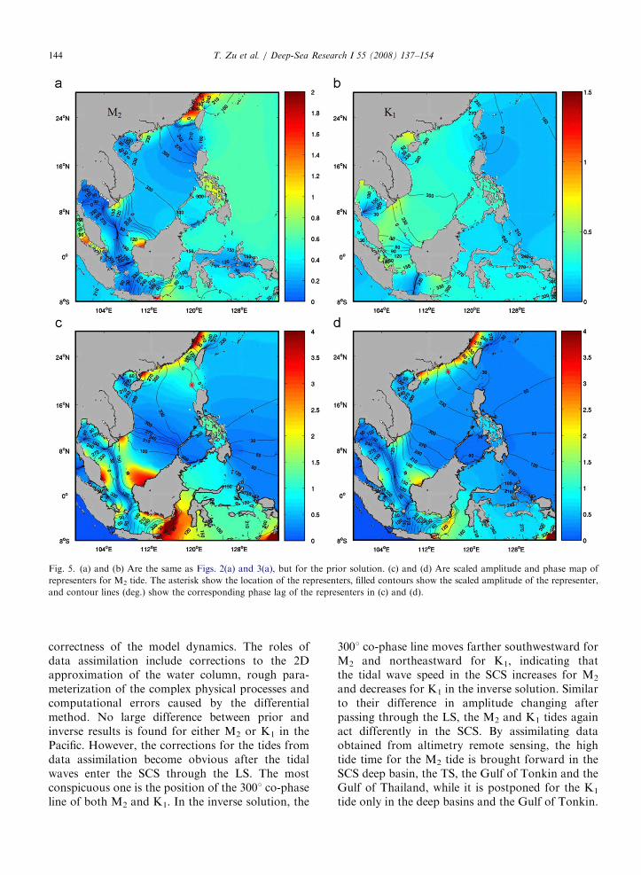
Fig. 5. (a) and (b) Are the same as Figs. 2(a) and 3(a), but for the prior solution. (c) and (d) Are scaled amplitude and phase map of

representers for M2 tide. The asterisk show the location of the representers, filled contours show the scaled amplitude of the representer,

and contour lines (deg.) show the corresponding phase lag of the representers in (c) and (d).

T. Zu et al. / Deep-Sea Research I 55 (2008) 137–154144

correctness of the model dynamics. The roles ofdata assimilation include corrections to the 2Dapproximation of the water column, rough para-meterization of the complex physical processes andcomputational errors caused by the differentialmethod. No large difference between prior andinverse results is found for either M2 or K1 in thePacific. However, the corrections for the tides fromdata assimilation become obvious after the tidalwaves enter the SCS through the LS. The mostconspicuous one is the position of the 3001 co-phaseline of both M2 and K1. In the inverse solution, the

3001 co-phase line moves farther southwestward forM2 and northeastward for K1, indicating thatthe tidal wave speed in the SCS increases for M2

and decreases for K1 in the inverse solution. Similarto their difference in amplitude changing afterpassing through the LS, the M2 and K1 tides againact differently in the SCS. By assimilating dataobtained from altimetry remote sensing, the hightide time for the M2 tide is brought forward in theSCS deep basin, the TS, the Gulf of Tonkin and theGulf of Thailand, while it is postponed for the K1

tide only in the deep basins and the Gulf of Tonkin.

ARTICLE IN PRESST. Zu et al. / Deep-Sea Research I 55 (2008) 137–154 145

On condition that the errors in the satelliteobservations are small enough, we could thinkthat the changes between the prior and inversesolutions are caused mainly by the large bottomtopography gradient and the coarse parameteriza-tion of the bottom friction coefficient. However, themost conspicuous change between the prior andinverse solutions in the SCS basin is probablycaused by the inclusion of baroclinicity, i.e., theinternal tide in the inverse flow field. Many studies(Jan et al., 2007; Niwa and Hibiya, 2004; Tian et al.,2003; Egbert and Ray, 2000) have pointed out thatinternal tides are generated in the LS and thecontinental shelf on the ECS with huge tidal energydissipation.

Figs. 5(c) and (d) show examples of representerfor the M2 constituent measured at the sites west ofthe LS and the continental edge of northern shelf,respectively. Following Foreman et al. (2004), thevalues of amplitudes and phase are scaled withrespect to the values of the measured sites. Theresults at both sites suggest that large amplitudes ofthe representers are mainly on the shelf, where wateris shallow, and in the slope, where topographygradient is large.

3.5. Model results validation

Simulated tidal harmonic constants are comparedwith those observation data obtained from tidalstations in the SCS. The comparison results for M2

and K1 tidal components are listed in Table 1.Differences between their amplitudes and phase lagsare calculated as distances in the complex plane(Foreman et al., 1993)

d ¼

ffiffiffiffiffiffiffiffiffiffiffiffiffiffiffiffiffiffiffiffiffiffiffiffiffiffiffiffiffiffiffiffiffiffiffiffiffiffiffiffiffiffiffiffiffiffiffiffiffiffiffiffiffiffiffiffiffiffiffiffiffiffiffiffiffiffiffiffiffiffiffiffiffiffiffiffiffiffiffiffiffiffiffiffiffiffiffiffiffiffiffiffiffiffiffiffiffiffiffiffiffiffiffiffiffiffiffiffiffiffiffiffiðHO cos gO �HS cos gSÞ

2þ ðHO sin gO �HS sin gSÞ

2

q,

where HO, gO, HS and gS are the observed andsimulated amplitudes and phase lags. The RMSerror of the complex amplitude isffiffiffiffiffiffiffiffiffiffiffiffiffiffiffiffiffiffiffiffiffiffiffiffiffiffiffiffiffiffiffiffiffiffiffiffiffiffiffiffiffiffiffi1

2N

XN

i¼1

jHSi �HOij2;

vuut

where N is the number of the observation stations,HSi is the model simulated amplitude at station i

and HOi is the amplitude from observation data atstation i.

Observation data are those first composed byFang et al. (1999) and used by Hu et al. (2001) andCai et al. (2006) based on two sources of data. Data

from the stations along the coasts of the mainlandof P.R. China, Hainan Island and Yongshujiaotaken from the archives of the Institute of Oceanol-ogy, the Chinese Academy of Sciences are generallybased on at least a full year of observations. Therest of the stations are quoted from the BritishAdmiralty Tide and Tidal Stream Tables, and theirdata quality varies (Fang et al., 1999). In ourcomputational domain, we randomly selected 55observation stations from these two sources of data.Simulated harmonic constants at the observationstations are interpolated or extrapolated by those onthe nearest model grids. The results are presented inTable 1.

In general, the results obtained in this study withthe GI scheme are improved in comparison with theresults along these coastal stations from theprevious studies. The RMS error of the complexamplitude of M2 and K1 for our result is (4.29, 2.15)as shown in Table 1, and were (11.64, 4.39), (17.58,3.59), (5.01, 2.58) for Fang et al. (1999), Hu et al.(2001), and Cai et al. (2006), respectively. FromTable 1 and Figs. 2(a) and 3(a), it is not difficult todiscover that most improved stations are focused onthe left and right sides of the SCS basin, between 61and 181N, where the co-phase lines of both M2 andK1 are sparse and their co-amplitude lines do notvary much. The station where the simulation datacompares most favorably with the observation datais Yongshujiao (Fig. 6), located south of the centralSCS basin (Fig. 1), and where the d of M2, K1 are0.21 and 1.57, respectively. In other words, the tidalwaves are well reproduced in the deep basin.However, the results at stations on the shallowcontinental shelves and in the gulfs, where theaccuracy of the tidal wave is highly dependent onthe veracity of the coastal topography, are notimproved as much as those along basin edges or inthe open ocean, as compared with previous results.In general, the model’s performance on shallowcontinental shelves, where the tidal features arecomplicated, with densely distributed co-phase linesand variable co-amplitude lines, is not as good asthat around the deep SCS basin. For example, the d

of M2 and K1 is 10.62 and 10.92 at Hong Kong,23.87 and 6.08 at Kuching, much larger than that atYongshujiao. Insufficient model resolution over theshelves is one of the possible reasons. Since thecomplex coastlines still could not be well resolved bythe present model, small tidal features around theobservation stations along the coasts and near theislands might not be represented. In addition,

ARTIC

LEIN

PRES

S

Table 1

Comparison of the harmonic constant between observation and calculated results

Station name Latitude Longitude M2 K1

Observation Calculation Absolute error Relative

error (%)

d Observation Calculation Absolute error Relative

error (%)

d

H

(cm)

g

(deg.)

H g dH dg H g H g dH dg

1 Xiamen 241270 1181040 184 352 168.5 351.3 �15.5 �0.7 8.42 0.20 15.65 34 281 32.2 282.4 �1.8 1.4 5.29 0.50 1.97

2 Hong Kong 221180 1141100 37 256 37.4 272.4 0.4 16.4 1.08 6.41 10.62 36 297 36.2 314.4 0.2 17.4 0.56 5.86 10.92

3 Lingshuijiao 181230 1101040 18 310 19.9 304.9 1.9 �5.1 10.56 1.65 2.54 30 317 32.7 316 2.7 �1 9.00 0.32 2.75

4 Basuo 191060 1081370 18 61 17.6 66.6 �0.4 5.6 2.22 9.18 1.78 54 71 55 74.3 1 3.3 1.85 4.65 3.29

5 Beihai 211290 1091050 44 177 43.1 177.5 �0.9 0.5 2.05 0.28 0.98 88 96 88.1 101.7 0.1 5.7 0.11 5.94 8.76

6 Tsieng mum 211080 1071370 18 179 19.4 173.4 1.4 �5.6 7.78 3.13 2.30 73 96 79.1 101.6 6.1 5.6 8.36 5.83 9.61

7 Thuan An 161340 1071380 18 351 19.1 350.5 1.1 �0.5 6.11 0.14 1.11 3 270 4.2 302.4 1.2 32.4 40.00 12.00 2.32

8 Da Nang 161050 1081110 17 330 17 319.2 0 �10.8 0.00 3.27 3.20 20 304 23.6 301.8 3.6 �2.2 18.00 0.72 3.70

9 Qui Nhon 131450 1091130 18 321 17.5 312.3 �0.5 �8.7 2.78 2.71 2.74 34 315 32.7 311.4 �1.3 �3.6 3.82 1.14 2.47

10 Nha Trang 121120 1091120 18 321 17.9 317.9 �0.1 �3.1 0.56 0.97 0.98 34 307 33.8 311.8 �0.2 4.8 0.59 1.56 2.85

11 Cam Ranh 111530 1091120 18 329 18.5 320 0.5 �9 2.78 2.74 2.91 34 307 34.3 311.3 0.3 4.3 0.88 1.40 2.58

12 Con Dao 81400 1061380 79 81 71 82.9 �8 1.9 10.13 2.35 8.38 64 333 59 339.7 �5 6.7 7.81 2.01 8.75

13 Ream 101300 1031360 7 29 6.4 12.8 �0.6 �16.2 8.57 55.86 1.98 22 135 19.7 124.8 �2.3 �10.2 10.45 7.56 4.36

14 KaohKong Is. 111250 1031000 12 51 9.4 24 �2.6 �27 21.67 52.94 5.60 37 161 34.7 161 �2.3 0 6.22 0.00 2.30

15 Satahib bay 121390 1001550 24 159 21 160.5 �3 1.5 12.50 0.94 3.06 64 176 62.5 180.7 �1.5 4.7 2.34 2.67 5.40

16 Bangkok bar 131280 1001350 55 170 40.7 184.7 �14.3 14.7 26.00 8.65 18.74 67 182 73.3 188.7 6.3 6.7 9.40 3.68 10.33

17 Ko Reat 111480 991490 6 168 6.8 170.3 0.8 2.3 13.33 1.37 0.84 52 184 52.1 181.8 0.1 �2.2 0.19 1.20 2.00

18 Tumpat 61120 1021100 18 261 16.2 247.3 �1.8 �13.7 10.00 5.25 4.45 28 351 25.3 346.8 �2.7 �4.2 9.64 1.20 3.33

19 Trengganu 51210 1031080 27 243 26.3 237.4 �0.7 �5.6 2.59 2.30 2.70 52 3 48.8 1.4 �3.2 �1.6 6.15 53.33 3.50

20 Kuantan 31500 1031200 55 270 55.19 262 0.19 �8 0.35 2.96 7.69 52 18 52.4 13.4 0.4 �4.6 0.77 25.56 4.21

21 Pulau Laut 41450 1081000 9 85 14.7 80.4 5.7 �4.6 63.33 5.41 5.77 36 348 41.5 343 5.5 �5 15.28 1.44 6.45

22 Natuna 31480 1081020 21 117 21 106.9 0 �10.1 0.00 8.63 3.70 40 355 36.5 352.9 �3.5 �2.1 8.75 0.59 3.77

23 Subi Kechil 31030 1081510 49 109 44.9 103.8 �4.1 �5.2 8.37 4.77 5.91 37 350 35.5 344.1 �1.5 �5.9 4.05 1.69 4.02

T.

Zu

eta

l./

Deep

-Sea

Resea

rchI

55

(2

00

8)

13

7–

15

4146

ARTIC

LEIN

PRES

S24 Tangjong Datu 21050 1091390 91 117 113.2 117.1 22.2 0.1 24.40 0.09 22.20 37 335 45.6 340.4 8.6 5.4 23.24 1.61 9.43

25 Batang Mukah 21540 1121050 37 93 33.9 88.2 �3.1 �4.8 8.38 5.16 4.29 40 326 44.1 323.9 4.1 �2.1 10.25 0.64 4.38

26 Miri 41230 1131590 15 341 15.8 335.7 0.8 �5.3 5.33 1.55 1.63 37 324 36.9 315.3 �0.1 �8.7 0.27 2.69 5.61

27 Labuan 51170 1151150 27 322 26 322.8 �1 0.8 3.70 0.25 1.07 40 320 38.2 317.3 �1.8 �2.7 4.50 0.84 2.58

28 Kota Kinabalu 51520 1151590 23 314 27.7 325.9 4.7 11.9 20.43 3.79 7.03 35 314 37.7 318.8 2.7 4.8 7.71 1.53 4.07

29 Balabak Is. 81000 1171040 24 314 21.3 311.6 �2.7 �2.4 11.25 0.76 2.86 30 323 34.2 314.3 4.2 �8.7 14.00 2.69 6.42

30 Ulugan bay 101040 1181460 21 304 19.4 303.4 �1.6 �0.6 7.62 0.20 1.61 34 317 31.8 313.6 �2.2 �3.4 6.47 1.07 2.94

31 Kulion Is. 111480 1191570 24 303 23.5 300.9 �0.5 �2.1 2.08 0.69 1.00 30 318 31.9 317.2 1.9 �0.8 6.33 0.25 1.95

32 Lubang Is. 131490 1201120 20 290 16.5 292 �3.5 2 17.50 0.69 3.56 29 310 29.1 313.3 0.1 3.3 0.34 1.06 1.68

33 Olongapo 141490 1201170 17 287 15.2 290.1 �1.8 3.1 10.59 1.08 2.00 27 316 28.3 313.8 1.3 �2.2 4.81 0.70 1.68

34 Santa Cruz 151460 1191540 12 263 12.8 285.3 0.8 22.3 6.67 8.48 4.86 26 313 26.9 314 0.9 1 3.46 0.32 1.01

35 San Fernando 161370 1201180 8 264 9.5 268.3 1.5 4.3 18.75 1.63 1.64 24 312 23.5 315.2 �0.5 3.2 2.08 1.03 1.42

36 Yongshujiao 91330 1121530 18 319 17.8 318.9 �0.2 �0.1 1.11 0.03 0.20 35 311 34.3 313.4 �0.7 2.4 2.00 0.77 1.61

37 Makung 231230 1191340 87 326 95.8 326.2 8.8 0.2 10.11 0.06 8.81 25 278 24.5 276.8 �0.5 �1.2 2.00 0.43 0.72

38 Kaohsiung 221370 1201160 15 236 19.9 211.7 4.9 �24.3 32.67 10.30 8.77 16 295 18.5 283 2.5 �12 15.63 4.07 4.38

39 Taichung 241110 1201290 148 327 163.8 317.8 15.8 �9.2 10.68 2.81 29.55 18 268 23.4 264.5 5.4 �3.5 30.00 1.31 5.54

40 Shaoanwan 231360 1171060 76 14 76.5 14.71 0.5 0.71 0.66 5.07 1.07 34 292 30.7 291.2 �3.3 �0.8 9.71 0.27 3.33

41 Shantou 231200 1161450 41 22 45.1 16.12 4.1 �5.88 10.00 26.73 6.02 29 297 29.3 292.2 0.3 �4.8 1.03 1.62 2.46

42 Shanwei 221450 1151210 28 255 25 246.5 �3 �8.5 10.71 3.33 4.94 33 298 32.4 296.3 �0.6 �1.7 1.82 0.57 1.14

43 Dayawan 221440 1141440 37 252 36.8 253.1 �0.2 1.1 0.54 0.44 0.74 34 295 36.1 302.8 2.1 7.8 6.18 2.64 5.21

44 Hailingshan 211350 1111490 68 294 54.6 276 �13.4 �18 19.71 6.12 23.30 42 314 38.7 312.7 �3.3 �1.3 7.86 0.41 3.42

45 Haikou 201010 1101170 20 264 23.9 253.2 3.9 �10.8 19.50 4.09 5.67 39 96 36.7 91.2 �2.3 �4.8 5.90 5.00 3.92

46 Yangpu 191500 1091200 24 150 29 148.7 5 �1.3 20.83 0.87 5.04 73 85 78.9 90.8 5.9 5.8 8.08 6.82 9.68

47 Hon Nieu 181480 1051460 30 31 37.7 32.1 7.7 1.1 25.67 3.55 7.73 49 103 51 110.5 2 7.5 4.08 7.28 6.84

48 Quang Khe 171420 1061280 18 41 25.3 17 7.3 �24 40.56 58.54 11.49 21 110 25 107.1 4 �2.9 19.05 2.64 4.16

49 Vung Tau 101200 1071040 79 63 69.7 65.1 �9.3 2.1 11.77 3.33 9.69 61 327 55.6 327.5 �5.4 0.5 8.85 0.15 5.42

50 Hatien 101220 1041280 10 119 13 98.2 3 �20.8 30.00 17.48 5.09 26 81 23 79.5 �3 �1.5 11.54 1.85 3.07

51 Pulau Tionman 21480 1041080 58 274 62.9 272.7 4.9 �1.3 8.45 0.47 5.09 49 25 46.6 25.3 �2.4 0.3 4.90 1.20 2.41

52 Anamba Is. 31140 1061150 18 267 17.3 256.7 �0.7 �10.3 3.89 3.86 3.24 40 13 39 13.4 �1 0.4 2.50 3.08 1.04

53 Kuching 11340 1101210 149 131 150.9 121.9 1.9 �9.1 1.28 6.95 23.87 47 348 48.7 341 1.7 �7 3.62 2.01 6.08

54 Kuala Paloh 21270 1111140 110 114 116.7 117.8 6.7 3.8 6.09 3.33 10.07 46 338 46.5 336.3 0.5 �1.7 1.09 0.50 1.46

55 Putai 231230 1201090 60 312 62.1 307.8 2.1 �4.2 3.50 1.35 4.94 20 278 20.4 274.3 0.4 �3.7 2.00 1.33 1.36

averarge absolute error 0.46 �3.81 0.43 0.31

RMS error of complex amplitude 4.29 2.15

g is the local phase lag, 8 h before GMT at 1201E.

T.

Zu

eta

l./

Deep

-Sea

Resea

rchI

55

(2

00

8)

13

7–

15

4147

ARTICLE IN PRESS

Fig. 6. Tidal elevation predictions from the model results and the observation data based on M2 S1 K1 and O1 constituents for the

Yongshujiao station.

T. Zu et al. / Deep-Sea Research I 55 (2008) 137–154148

omitting non-linear terms in the data assimilationpart might also compromise the accuracy of themodel results, as non-linear interactions betweentidal constituents are sometimes important inshallow waters. The figures in Table 1 also showthat the results for K1 are better than those for M2

in the TS, because the strong M2 tide is highlysensitive to the local topography. On the contrary,results for M2 are better than those for K1 at thenorthern part of the Gulf of Tonkin.

4. Tidal energy and dynamic discussion

To understand the tidal dynamics and to explainthe mechanism of the processes of the M2 and K1

tides, the distribution of tidal energy in the SCS isinvestigated in this section. Following Garrett(1975), the energy equation is obtained by thenon-linear equations in the prior model. Adding(2.1)~v and (2.2)gz, we have

qE

qtþ r � ðg~UzÞ ¼ g~U � rðzSAL þ zEÞ � F �~v� ð~U � r~vÞ �~v

þHAh~v � r2~v, ð4:1Þ

where E ¼ ð1=2ÞH~v2 þ ð1=2Þgz2 denotes the energydensity. Assuming that qE=qt ¼ 0 and (4.1)� r and

averaged over a tidal cycle, then (4.1) becomes

W � r � P ¼ DþN � L, (4.2)

where W ¼ rg U � rðzSAL þ zEÞ� �

is the work ratedone by the tidal generating force, P ¼ rg/UzSdenotes the tidal energy flux, r � P represents thedivergence of the energy flux, D ¼ r F �~vh i denotesthe tidal dissipation rate caused by the bottomfriction, N ¼ ð~U � r~vÞ �~v is the work rate by thenon-linear interaction, L ¼ HAh~v � r

2~v is the dis-sipation caused by the lateral friction, and /Sdenotes time average.

In the data assimilation calculation, the energyEq. (4.2) can be written as

W � r � P ¼ DþN þ LþD0, (4.3)

where D0 denotes the residuals in the momentumequation. When the numerical techniques areassumed reasonably accurate, D0 is mostly due tothe incomplete and inaccurate physics prescribed inthe dynamic equation, probably arising from someuncertain dissipation processes, such as theenergy transformation from barotropic tide intothe internal tide, etc. Other terms are the same asthose in Eq. (4.2).

ARTICLE IN PRESST. Zu et al. / Deep-Sea Research I 55 (2008) 137–154 149

4.1. Tidal energy distribution

The values of P, r � P and W calculated from(4.3) are shown in Figs. 7–9, respectively. FromFig. 7, we could see that southeast of LS in thePacific; the directions of the M2 and K1 tidal energyflux are quite different. The M2 energy fluxes arenorthward and northwestward, while the K1 energyfluxes are southwestward. In the northeast of the

Fig. 7. Vectors of tidal energy flux (P) for M2 and K1

Fig. 8. Divergence of the tidal

LS, the tidal energy fluxes of both M2 and K1 areamplified as the tidal waves approach the 3000-misobath from the open ocean. The directions of P

for both M2 and K1 shift southwestward bythe southwest–northeast oriented isobaths northeastof the TS. Only the stronger M2 energy flux isable to cross this topographical trench (Ryukyutrench) and propagates northward into the ECS,while the energy flux of K1 is guided mainly by the

. Contours denote the magnitude of P (W/m).

energy flux, , �P (W/m2).

ARTICLE IN PRESS

Fig. 9. The work rate done by the tidal generating force, W (W/m2).

T. Zu et al. / Deep-Sea Research I 55 (2008) 137–154150

local topography and propagates southwestward.The maximum M2 and K1 energy fluxes reach2� 105 and 1.5� 105W/m, respectively, in the LS,and the westward vectors of both the M2 and K1

energy fluxes suggest that the energy fluxes enter theSCS from the Pacific through the LS. On the east sideof the LS, the magnitude of both M2 and K1 tideenergy fluxes are larger than those on the west side ofthe LS, indicating the loss of energy while tidal wavespassing through the LS. In addition, only M2 energyflux is able to intrude into the SCS through the TS.Inside the SCS, both tidal waves propagatesouthwestward, which are in accordance with thecotidal charts. However, the magnitude of the M2

energy flux is weaker than that of K1 inside the SCS,while the opposite state occurs around the east of andin the LS.

The different characteristics of the M2 andK1 energy fluxes are associated with the work rateof the tidal generating force, energy divergence anddissipation around the LS, and with the directionsof the tidal energy flux east of the LS affected by theexistence of the northeast–southwest orientatedsteep Ryukyu trench. The divergence of the tidalenergy fluxes is tightly correlated with the bottomtopography (Fig. 8), as shown by the concomitantappearance of the strong energy flux divergence andconvergence over the complex and sharply changedtopography, such as the Ryukyu trench northeast ofTaiwan, the narrow steep straits and the Zhongsha,

Nansha archipelago inside the SCS basin. Fig. 8(a)shows that the LS and the TS are two regions withthe strongest M2 energy flux convergence. Thevalues of r � P in these two regions are more than�0.1W/m2, about five times of the values of W

(see below). According to (4.3), it suggests thatstrong M2 tidal energy dissipation occurs in theLS and the TS. Since the LS is also a mainconvergent zone for the K1 tidal energy flux(Fig. 8(b)), it could be regarded as a pump thatabsorbs and dissipates the tidal energy coming fromthe Pacific. On the west side of the LS in the SCSbasin, there exists a relatively large convergent/divergent area (about 0.03–0.06W/m2) of theM2/K1 tides, with the existence of the largernegative/positive work rate in the area (Fig. 9),suggesting that the M2/K1 tidal energy is reduced/amplified in this region.

A positive W denotes energy gain from the workof the tidal generating force, and a negative W

denotes energy loss while work is done against thetidal generating force. Fig. 9 shows that W is nearzero on most of the continental shelves. A large areaof positive work rate of the M2 tidal generatingforce, W, occurs in the Pacific basin (about0.003–0.01W/m2). The areas of positive W for theK1 tide in the Pacific are smaller than that for M2,and mainly located along the 3000-m isobath east ofTaiwan, where negative W is dominant for M2. Theamplified negative value (about �0.02W/m2) of the

ARTICLE IN PRESST. Zu et al. / Deep-Sea Research I 55 (2008) 137–154 151

M2 work rate occurs around the LS and in both thenorthern and southern parts of the TS, suggestingthat considerable M2 energy is lost there to the tidalgenerating force. The W distribution for the K1 tidein the LS is closely related to the bottom topo-graphy. Regions with negative work rates are foundin the shallower areas, while those with positivework rates exist in the deep channel between the twoshallower areas. West of the LS in the SCS basin,W is negative for M2 and positive for K1. Themaximum value of W for K1 is over 0.015W/m2.Without showing the distribution of W Ye andRobinson (1983) pointed out that the work doneby tidal generating force in the SCS was negativefor both M2 and K1, while Fang et al. (1999)showed that the W in the SCS basin was negativefor M2 and positive for K1, in accordance withour results. The spatial distribution of W aroundthe LS also suggests that while propagating fromeast of the LS into the SCS, the M2 tidecontinuously loses energy, and the K1 tide gainsenergy from the tidal generating force except in thetwo small shallower areas in the LS. Therefore, thecontrary behavior of the work rate of M2 and K1

tidal generating forces might be another factor thatexplains why M2 and K1 tides act quite differentlyinside the SCS.

The distribution of bottom friction dissipation,D, has also been calculated for the M2 and K1 tide(not shown). The results show strong D in shallowareas with large tidal currents, such as in the TS forM2 and in the gulf of Tonkin for K1, which is closelyrelated to the distribution of tidal current ellipsesshown in Figs. 2(b) and Fig. 3(b). However, no largearea of strong D is seen in LS. Since the magnitudesof N and L are 2–3 times smaller than r � P, thelarge energy dissipation (as defined in Egbert andRay (2000), i.e. W � r � P) in the LS is mostlybalanced by D0 in (4.3), and it could be consideredas the correction to the prior model, which couldnot take into account the conversion of barotropictidal energy into internal tide.

Additional information about the tide energy canbe obtained by comparing the energy flux resultsfrom the prior and inverse model. The obviousdifferences are found in the region around the LS(Fig. 10). The magnitudes of tidal energy fluxes ofboth M2 and K1 in the prior results reaching the LSfrom the Pacific are weaker than those from theinverse results, but the opposite conditions occur onthe west side of the LS. This evidently suggests thatmore energy of M2 and K1 is lost after crossing the

LS when the inverse scheme is applied. Quantita-tively, the energy budget across LS is estimated by theenergy flux into/out of the box shown in Fig. 10(a).The box is divided into SCS (left box) and Pacific(right box) parts by the central dashed line, represent-ing energy going out of and coming into the box. Inthe inverse (prior) calculation, for M2 tide, 48.71(41.79) GW energy flows into the right box, and 26.05(35.20) GW energy flows out of the left box, with22.66 (6.59) GW being dissipated in LS. For K1 tide,44.10 (28.48) GW energy flows into the right box, and19.17 (24.79) GW energy flows out of the left box,with 23.93 (3.69) GW being dissipated in LS. It isobvious that much more energy is dissipated in LS inthe inverse calculation. One possible explanation isthe conversion of the barotropic tides into the internaltides in the inverse results (Egbert, 1997; Egbert andRay, 2000; Niwa and Hibiya, 2004). From anotherpoint of view, to better understand the dynamicprocess of tides in areas of such complex topographyas the LS, a three-dimensional (3D) model is required.From the above analyses, it is conceivable that theweakened tide energy flux in the SCS after crossingthe LS is caused mainly by the strong tidal dissipationoccurring in the strait for K1 and the co-effect ofenergy lost in working against W and strong tidaldissipation for M2.

5. Summary

To study the tide and tidal energy in the SCS,T/P altimetry data have been assimilated into abarotropic ocean tide model by using OTIS. Itsolves the non-linear shallow water equation bytime stepping to get the prior results and then itlinearizes the equations and uses the advanced GImethod in the data assimilation calculation to getthe inverse results. The combination of largeamounts of T/P data with the dynamically well-defined equations are a good way to improvethe accuracy of tidal modeling by diminishingproblems such as the uncertainties in shallow watersand coastal areas caused by analyzing only theT/P data and the inaccuracies caused by merelysolving the dynamic equations with rough para-meterization of the coefficients. Additionally, highresolution and large model domain are applied inour study, which also improve the accuracy of themodeling. Reasonably good results are therebyobtained.

Results show that the M2 and K1 tides propagateinto the SCS through the LS and that they mainly

ARTICLE IN PRESS

Fig. 10. The tidal energy flux at the Luzon Strait, (a) the inverse and (b) the prior results for M2. Similarly, (c) and (d) are for K1. Contours

denote the magnitude of P (W/m).

T. Zu et al. / Deep-Sea Research I 55 (2008) 137–154152

continue propagating southwestward along the axisof the SCS basin. The M2 tidal amplitude is reducedwhile the K1 amplitude is amplified after they passthrough the LS, mainly because of the Helmholtzresonance. The tidal amplitude distribution and thecurrent fields are also closely related to the bottomtopography. Tidal characteristics are quite differenton the shallow continental shelves and in the deepwaters. The tidal waves propagate fast in the deepocean and slow on the continental shelves, while thetidal currents are strong and complex on the shelfareas and weak and regular in the deep waters.The co-phase lines are rather complex in shallowareas; several amphidromic systems exist on thecontinental shelf areas and in the two gulfs. Energy

studies show that on the eastern side of Luzon in thePacific, the northwestward M2 energy flux isfavorable for the intrusion into the ECS, whilethe southwestward K1 energy flux is favorablefor the intrusion into the SCS. Furthermore, thestudies reveal that the magnitudes of the workrate of the tidal generating forces, the divergenceof the energy flux and the energy dissipationare amplified in the LS and the TS. Both M2

and K1 tidal energies are dissipated most in the LSover the sharply varied bottom topography, indicat-ing the strong control of the topography overthe tidal energy distribution. The work rate fromthe tidal generating force in the SCS basin isnegative for M2 and positive for K1. The strong

ARTICLE IN PRESST. Zu et al. / Deep-Sea Research I 55 (2008) 137–154 153

negative W of M2 in the LS also explains whyso much M2 energy is lost while the tide passesthrough the LS into the SCS. It can be summarizedthat the different features of M2 and K1 in theSCS are highly associated with the different direc-tions of energy flux in the Pacific, which isunfavorable for the intrusion of M2 tidal energyinto the SCS but favorable for the K1 tide; andwith the tidal energy losses in M2 and gains in K1

from W inside the SCS basin. The different M2 andK1 behaviors in the SCS are also largely associatedwith the Helmholtz resonance in K1.

Acknowledgments

The authors are grateful to Gary Egbert, Jilan Su,Chris Garrett and Richard Ray for their help.Thoughtful comments and suggestions from twoanonymous reviewers, which led to many improve-ments in the manuscript, are appreciated. Thisresearch was supported by the Research GrantsCouncil of Hong Kong under Grants CERG-601204, CERG-601105 and CERG-601006.

References

Cai, S., Long, X., Liu, H., Wang, S., 2006. Tide model evaluation

under different conditions. Continental Shelf Research 26

(2006), 104–112.

Chao, S.Y., Shaw, P.T., Wu, S.Y., 1996. Deep water ventilation

in the South China Sea. Deep-Sea Research I 43 (4),

445–466.

Chu, P.C., Edmons, N.L., Fan, C.W., 1999. Dynamical mechan-

isms for the South China Sea seasonal circulation and

thermohaline variability. Journal of Physical Oceanography

29, 2971–2989.

Dietrich, G., 1944. Die Gezeiten des Weltmeeres als geograph,

Erseheinung Z. d. ges. Erdkunde, Berlin, 69pp.

Egbert, G.D., 1997. Tidal data inversion: interpolation and

inference. Progress in Oceanography 40, 81–108.

Egbert, G.D., Erofeeva, S.Y., 2002. Efficient inverse modeling of

barotropic ocean tides. Journal of Atmospheric and Oceanic

Technology 19 (2), 183–204.

Egbert, G.D., Ray, R.D., 2000. Significant dissipation of tidal

energy in the deep ocean inferred from satellite altimeter data.

Nature 405, 775–778.

Egbert, G.D., Bennett, A.F., Foreman, M.G.G., 1994. TOPEX/

Poseidon tides estimated using a global inverse model.

Journal of Geophysical Research 99, 24821–24852.

Fang, G., Cao, D., Huang, Q., 1994. Numerical modeling of the

tide and tidal current in the South China Sea. Acta

Oceanologica Sinica 16 (4), 1–12 (in Chinese).

Fang, G., Kwok, Y.K., Yu, K., Zhu, Y., 1999. Numerical

simulation of principal tidal constituents in the South China

Sea, Gulf of Tonkin and Gulf of Thailand. Continental Shelf

Research 19, 845–869.

Foreman, M.G.G., Henry, R.F., Walters, R.A., Ballantyne,

V.A., 1993. A finite element model for tides and resonance

along the north coast of British Columbia. Journal of

Geophysical Research 98, 2509–2531.

Foreman, M.G.G., Sutherland, G., Cummins, P.F., 2004. M2

tidal dissipation around Vancouver Island: an inverse

approach. Continental Shelf Research 24 (2004), 2167–2185.

Gan, J., Li, H., Curchitser, E. N., Haidvogel, D. B., 2006.

Modeling South China Sea circulation: response to seasonal

forcing regimes. Journal of Geophysical Research 111,

C06034, doi:10.1029/2005JC003298.

Garrett, C., 1975. Tides in gulfs. Deep-Sea Research 22,

23–35.

Garrett, C., Cummins, P., 2005. The power potential of tidal

currents in channels. Proceedings of the Royal Society.

doi:10.1098/rspa.2005.1494.

Hu, J.Y., Kawamura, H., Hong, H., Qi, Y.Q., 2000. A review on

the currents in the South China Sea: seasonal circulation,

South China Sea warm current and Kuroshio intrusion.

Journal of Oceanography 56, 607–624.

Hu, J.Y., Kawamura, H., Hong, H.S., Kobashi, F., 2001.

Tidal features in the China Sea and their adjacent sea

areas as derived from TOPEX/POSEIDON altimeter data.

Chinese Journal of Oceanology and Limnology 19 (4),

293–305.

Jan, S., Chern, C.-S., Wang, J., Chao, S.-Y., 2007. Generation

of diurnal K1 internal tide in the Luzon Strait and

its influence on surface tide in the South China Sea,

Journal of Geophysical Research 112, C06019, doi:10.1029/

2006JC004003.

Morozov, E.G., 1995. Semidiurnal internal wave global field.

Deep-Sea Research I 42, 135–148.

Munk, W.H., Wunsch, C., 1998. Abyssal recipes II: energetics

of tidal and wind mixing. Deep-Sea Research I 45,

1977–2010.

Niwa, Y., Hibiya, T., 2004. Three-dimensional numerical

simulation of M2 internal tides in the East China Sea,

J. Geophysical Research 109 (C04027).

Ray, R.D., 1998. Ocean self-attraction and loading in numerical

tidal models. Marine Geodesy 21, 181–192.

Sergeev, J.N., 1964. The application of the method of marginal

values for the calculation of charts of tidal harmonic

constants in the South China Sea. Okeanologiia 4, 595–602

(in Russian, English abstract).

Shaw, P.T., Chao, S.Y., 1994. Surface circulation in the South

China Sea. Deep-Sea Research I 40 (11/12), 1663–1683.

Sutherland, G., Garrett, C., Foreman, M.G.G., 2005. Tidal

resonance in Juau de Fuca Strait and the Strait of Georgia.

Journal of Physical Oceanography 35, 1279–1286.

Tian, J., Zhou, L., Zhang, X., Liang, X., Zheng, Q., Zhao, W.,

2003. Estimates of M2 internal tide energy fluxes along the

margin of Northwestern Pacific using TOPEX/POSEIDON

altimeter data. Journal of Geophysical Research 30 (17),

1889.

Wyrtki, K., 1961. Physical oceanography of the Southeast Asian

water. In NAGA Report Vol. 2, Scientific Result of Marine

Investigation of the South China Sea and Gulf of Thailand

1959–1961, Scripps Institution of Oceanography, La Jolla,

California, 195pp.

Xu, X.Z., Qiu, Z., Chen, H.C., 1982. The general descriptions

of the horizontal circulation in the South China Sea.

In: Proceedings of the 1980 Symposium on Hydrometeology

ARTICLE IN PRESST. Zu et al. / Deep-Sea Research I 55 (2008) 137–154154

of the Chinese Society of Oceanology and Limnology,

Science Press, Beijing (in Chinese with English abstract),

pp. 137–145.

Yanagi, T., Takao, T., Morimoto, A., 1997. Co-tidal and co-

range charts in the South China Sea derived from satellite

altimetry data. Lamer 35, 85–93.

Ye, A.L., Robinson, I.S., 1983. Tidal dynamics in the South

China Sea. Geophysical Journal of the Royal Astronomical

Society 72, 691–707.

Yu, M., 1984. A preliminary study of tidal characteristics in

the South China Sea. Acta Oceanologica Sinica 6, 293–300

(in Chinese).