NUMERICAL STUDY OF A TURBULENT HYDRAULIC JUMP

Qun Zhao 1 Shubhra K. Misra1

Ib A. Svendsen 1 (Member, ASCE) and James T. Kirby 1 (Member, ASCE)

ABSTRACTIn this paper, we describe the numerical simulation of a turbulent hydraulic jump. The numerical

model is based on RIPPLE (Kothe et al., 1994) with two turbulence closure submodels: the standardk− ε model of Launder and Spalding (1974) and a multi-scale k− l model of Zhao et al. (2004). Modelresults are compared to LDV data of Bakunin (1995) and Svendsen et al. (2000).

Keywords: hydraulic jump, bore, spilling breaker

INTRODUCTIONHydraulic jumps and bores are similar flows even though the hydraulic jump is stationary

and the bore is propagating. In fact a bore can be viewed and analyzed in a coordinate sys-tem moving at the bore propagation speed as a stationary hydraulic jump. Hydraulic jumpsare commonly used as energy dissipators and they have been studied intensively by hydraulicengineers mainly through laboratory experiments.

Hydraulic jumps and bores are also of interest to coastal engineers due to the similaritywith broken waves inside the surf zone (Peregrine and Svendsen, 1978, Madsen and Svendsen,1983). Spilling breakers are often modeled as a hydraulic jump with a stagnant eddy (roller)riding on the turbulent front face (Svendsen and Madsen, 1984). Most of the studies focusingon hydraulic jumps are however based on laboratory experiments and semi-analytical solutions(Svendsen et al., 2000). The numerical studies reported so far are mainly based on nonlinearshallow water equations (NSWE), where jumps and bores are considered as a discontinuity(shocks) of the water surface. An early study by Hibberd and Peregrine (1975) used a Lax-Wendroff scheme where the dissipation was implicitly represented in the numerical scheme.More advanced ”shock capture” methods such as Weighted Averaged Flux (WAF) method areused by recent NSWE solvers such as Brocchini et al.(2001) and Hubbard and Dodd (2002).However, as pointed out by Madsen and Svendsen (1983), these methods based on NSWE areunable to correctly describe the shape of the free surface and the velocities underneath it.

In the present work, we apply a Navier-Stokes solver based on the VOF method (Kothe etal., 1994, Zhao et. al 2004) to study a turbulent hydraulic jump. We will focus on the meanflow motions in the hydraulic jump. Another aspect that distinguishes the present study fromothers (such as Chippada et al., 1994; Liu and Drewes, 1995; Ma et al., 2002) is that in this

1Center for Applied Coastal Research, University of Delaware, Newark, DE 19716, USA. Corresponding authoremail: zhao@coastal.udel.edu, fax:302-831-1228

work we will focus on weak hydraulic jumps/bores, i.e., Froude number less than 2, due totheir similarity to the bores observed in the natural beach. At the first stage of this work, wewish to validate our numerical model using the laboratory measurements of Bakunin (1995)and Svendsen et al. (2000).

GOVERNING EQUATIONSThe numerical model used here is based on the two-dimensional VOF model RIPPLE

(Kothe et al., 1994). The governing equations are the continuity and momentum equationfor incompressible flow in the x − z plane,

∂uj

∂xj

= 0 (1)

∂ui

∂t+ uj

∂ui

∂xj

= −1

ρ

∂p

∂xi

+ ν∂2ui

∂xj∂xj

+ gi, (2)

where i = 1, 2 are indices in the x and z direction, respectively, and j is a repeated dummyindex. ν is the kinematic viscosity and gi the gravitational acceleration, where g1 = 0. p is thepressure, and ρ the fluid density with t the time. The pressure is solved using an incompleteCholesky conjugate gradient technique for the pressure Poisson equation.

The VOF method uses a ”volume of fluid” function F (x, z, t) to to track the motion of thefree surface. A unit value of F corresponds to a cell full of fluid, while a zero value indicatesthat the cell contains no fluid. Cells with F values between zero and one contain a free surface.The time evolution of F is governed by,

∂F

∂t+ uj

∂F

∂xj

= 0. (3)

The instantaneous equations (1)-(3) cannot be solved directly due to the high Reynoldsnumber and the limitation of the grid size. The governing equations are thus averaged overtime or space. Upon using the Boussinesq eddy viscosity assumption, the mean momentumequations read

∂ui

∂t+ uj

∂ui

∂xj

= −1

ρ

∂p

∂xi

+∂

∂xj

[(ν + νT )∂ui

∂xj

] + gi. (4)

where νT is the eddy viscosity. The variables with an overbar denote the mean variables eithertime-averaged or space-averaged depending on the turbulence model used.

TURBULENCE MODELING

The k − ε modelThe ”standard” k − ε model (Launder and Spalding, 1974; Rodi, 1980) is given by

∂K

∂t+ uj

∂K

∂xj

=∂

∂xj

(ν +νT

σK

∂K

∂xj

) + PROD − ε. (5)

∂ε

∂t+ uj

∂ε

∂xj

=∂

∂xj

(ν +νT

σε

∂ε

∂xj

) + ε(cε1PROD − cε2ε). (6)

where K and ε are the turbulent kinetic energy and dissipation rate. PROD denotes the pro-duction term due to the mean flow

PROD = νT

[

1

2

(∂ui

∂xj

+∂uj

∂xi

)(∂ui

∂xj

+∂uj

∂xi

)

]

, (7)

2

K 4K 2K 1

K N

εε2

1

3

ε4 εN−1

ε3

ε

4κ1 κ2

N

3 κN−1 κNκ

K

κ

K

κ

PROD

FIG. 1. Partition of the spectra density

and the eddy viscosity relates the kinetic energy and dissipation rate as

νT = cµK2

ε(8)

We use the ”standard coefficients” here: cu = 0.09, σK = 1.0, σε = 1.3, cε2 = 1.92,

cε1 = cε2 − κ2/σεc1

2µ .

The Multi-scale Turbulence ModelAs for the multi-scale turbulence model, we follow the work of Zhao et al. (2004) to set up

N levels of k − l equations, in which turbulent kinetic energy can be transferred from largerlength scales to smaller ones explicitly (see Figure 1). In this approach, the production termat the first level is dominated by the ”large eddies”, i.e., the smallest resolved scale (the gridscale, in this case),

PROD1 = νt1

[

1

2

(∂ui

∂xj

+∂uj

∂xi

)(∂ui

∂xj

+∂uj

∂xi

)

]

, (9)

The dissipation term is the k − l type dissipation,

εn = Cdk3

2n /ln, 1 ≤ n < N, (10)

where the length scale for each partition is

ln =

√∆x∆z

2n−11 ≤ n < N (11)

Within each partition n > 1, production is set equal to dissipation at the next n-level grid scalepartition,

PRODn = εn−1 2 ≤ n ≤ N. (12)

Then the total sub-grid scale (SGS) turbulent kinetic energy is the sum of the kinetic energy inall partitions,

k = k1 + k2 + ... + kN = ΣNn=1kn. (13)

3

We also assume that turbulent kinetic energy leaves the system at the smallest scales, thereforethe total dissipation of the system is characterized as

ε = εN . (14)

Then the nth level k − l equation reads,

∂kn

∂t+ uj

∂kn

∂xj

=∂

∂xj

(νtn

σk

∂kn

∂xj

) + PRODn − εn. (15)

Cd = 0.2, Cs = 0.1 and σk = 1.0 are used in the present study.The eddy viscosity νtn at the nth level is set to all the scales smaller than n,

νtn = ΣNi=nCsk

1

2

i li 1 ≤ n < N. (16)

andνT = νt1 , (17)

in (4). For the results presented below, N = 3, i.e., three levels of k − l equations are solved.

NUMERICAL CONSIDERATIONSThe numerical scheme in this work follows RIPPLE (Kothe et al., 1994) and Zhao et al.

(2004). At the bottom boundary, we use the wall boundary condition (Launder and Spalding,1974) to match the near wall velocity to the ”wall function”. At inflow, we use the powerlaw velocity profile to approximate the velocity at the first measured point in the experiment.Downstream boundary condition is forced to conserve the volume flux.

PRELIMINARY RESULTS: THE MEAN QUANTITIES

0 1 2 3 4 5 6 7 8 9 100

0.5

1

1.5

x/h0

z/h 0

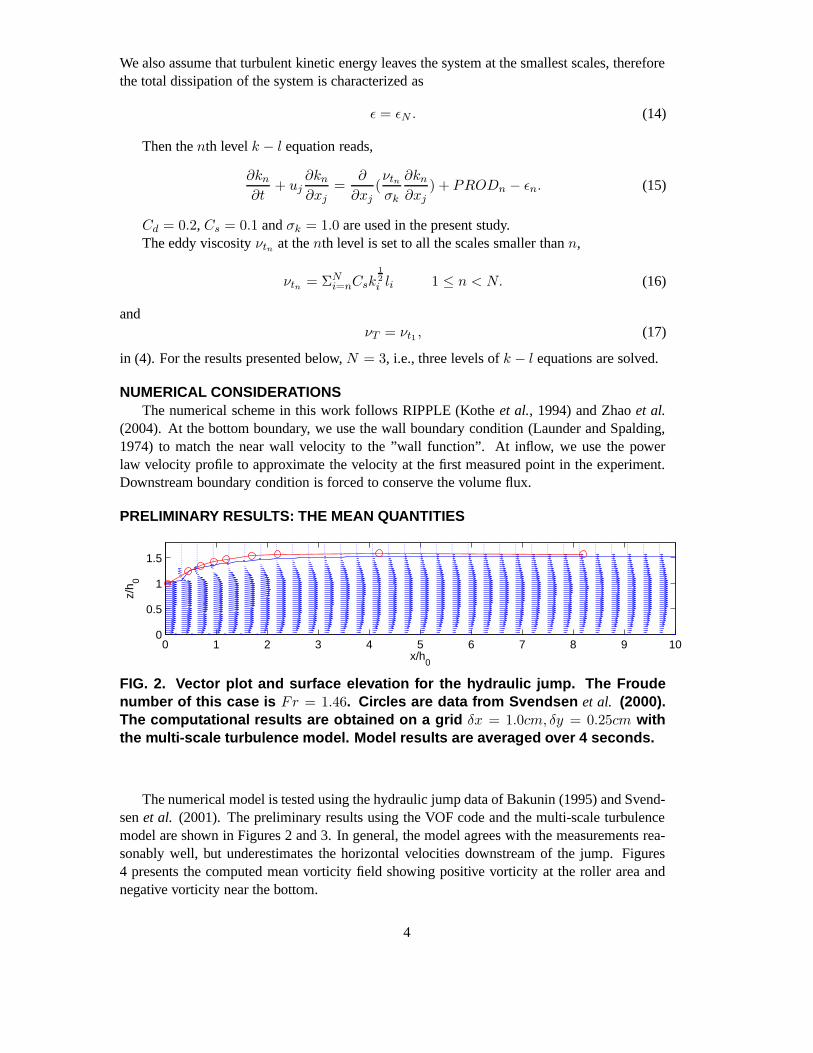
FIG. 2. Vector plot and surface elevation for the hydraulic jump. The Froudenumber of this case is Fr = 1.46. Circles are data from Svendsen et al. (2000).The computational results are obtained on a grid δx = 1.0cm, δy = 0.25cm withthe multi-scale turbulence model. Model results are averaged over 4 seconds.

The numerical model is tested using the hydraulic jump data of Bakunin (1995) and Svend-sen et al. (2001). The preliminary results using the VOF code and the multi-scale turbulencemodel are shown in Figures 2 and 3. In general, the model agrees with the measurements rea-sonably well, but underestimates the horizontal velocities downstream of the jump. Figures4 presents the computed mean vorticity field showing positive vorticity at the roller area andnegative vorticity near the bottom.

4

−50 0 50 1001500

0.5

1

1.5

gauge1

z/h 0

−50 0 50 1001500

0.5

1

1.5

gauge2

−50 0 50 1001500

0.5

1

1.5

gauge3

−50 0 50 1001500

0.5

1

1.5

gauge4

−50 0 50 1001500

0.5

1

1.5

gauge5

−50 0 50 1001500

0.5

1

1.5

gauge6

z/h 0

U(cm/s)−50 0 50 1001500

0.5

1

1.5

gauge7

U(cm/s)−50 0 50 1001500

0.5

1

1.5

gauge8

U(cm/s)−50 0 50 1001500

0.5

1

1.5

gauge9

U(cm/s)

FIG. 3. Comparison of measured (circles, Svendsen et al., 2000) and modeled(line, the multi-scale turbulence model) mean horizontal velocity profiles. Gaugelocations correspond to the circles in Figure 2.

SUMMARYThe preliminary results show that the numerical model agrees reasonably well with the

lab measurements for the mean flow. But the model underestimates the horizontal velocitiesdownstream of the jump. We are currently working on comparing the turbulent motions withthe measurements and hope to present those results at the conference.

ACKNOWLEDGMENTSThis work is supported by the National Oceanographic Partnership Program (NOPP), grant

N00014-99-1-1051.

REFERENCES

• Bakunin, J. (1995): Experimental study of hydraulic jumps in low Froude numberrange. MCE thesis, Department of Civil AND Environmental Engineering, Univer-sity of Delaware, Newark, DE 19711.

• Brocchini, M., R. Bernetti, A. Mancinelli and G. Albertini (2001): An efficient solverfor nearshore flows based on WAF method. Coastal Engineering, vol 43, pp. 105-129.

• Chippada, S., B. Ramaswamy and M. F. Wheeler (1994): Numerical simulation of hy-draulic jump. International Journal of Numerical Methods in Engineering. vol. 37, pp.

5

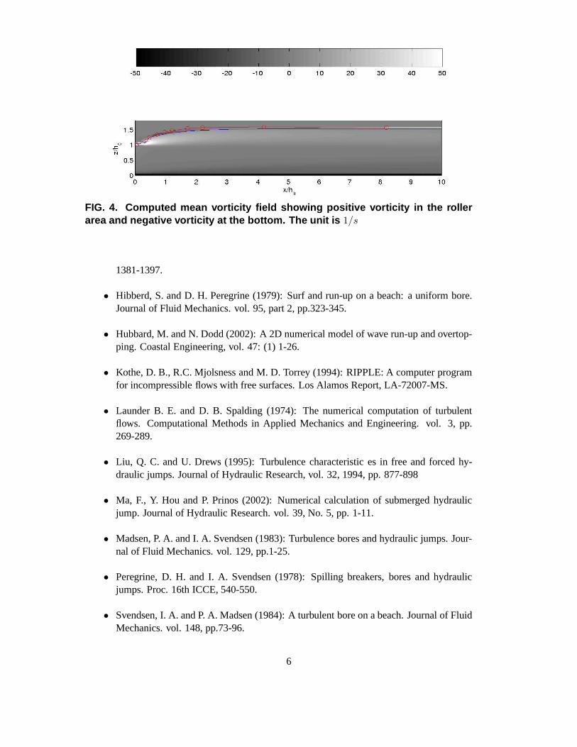
FIG. 4. Computed mean vorticity field showing positive vorticity in the rollerarea and negative vorticity at the bottom. The unit is 1/s

1381-1397.

• Hibberd, S. and D. H. Peregrine (1979): Surf and run-up on a beach: a uniform bore.Journal of Fluid Mechanics. vol. 95, part 2, pp.323-345.

• Hubbard, M. and N. Dodd (2002): A 2D numerical model of wave run-up and overtop-ping. Coastal Engineering, vol. 47: (1) 1-26.

• Kothe, D. B., R.C. Mjolsness and M. D. Torrey (1994): RIPPLE: A computer programfor incompressible flows with free surfaces. Los Alamos Report, LA-72007-MS.

• Launder B. E. and D. B. Spalding (1974): The numerical computation of turbulentflows. Computational Methods in Applied Mechanics and Engineering. vol. 3, pp.269-289.

• Liu, Q. C. and U. Drews (1995): Turbulence characteristic es in free and forced hy-draulic jumps. Journal of Hydraulic Research, vol. 32, 1994, pp. 877-898

• Ma, F., Y. Hou and P. Prinos (2002): Numerical calculation of submerged hydraulicjump. Journal of Hydraulic Research. vol. 39, No. 5, pp. 1-11.

• Madsen, P. A. and I. A. Svendsen (1983): Turbulence bores and hydraulic jumps. Jour-nal of Fluid Mechanics. vol. 129, pp.1-25.

• Peregrine, D. H. and I. A. Svendsen (1978): Spilling breakers, bores and hydraulicjumps. Proc. 16th ICCE, 540-550.

• Svendsen, I. A. and P. A. Madsen (1984): A turbulent bore on a beach. Journal of FluidMechanics. vol. 148, pp.73-96.

6

• Svendsen, I. A., Veeramony, J., Bakunin, J. and J. T. Kirby (2000): The flow in weakturbulent hydraulic jump. Journal of fluid Mechanics. vol 418, pp. 25-57.

• Zhao, Q., S. Armfield and K. Tanimoto (2004) : Numerical simulation of breakingwaves by a multi-scale turbulence model.Coastal Engineering 51, pp. 53-80.

7