Numerical Study of a Stratified Cold Water Storage956036/FULLTEXT01.pdf · Utan att ändra de andra...
118
Master of Science Thesis KTH School of Industrial Engineering and Management Energy Technology EGI-2016-038 Division of Heat and Power SE-100 44 STOCKHOLM Numerical Study of a Stratified Cold Water Storage Jean-François OLIVIER
Transcript of Numerical Study of a Stratified Cold Water Storage956036/FULLTEXT01.pdf · Utan att ändra de andra...

Master of Science Thesis KTH School of Industrial Engineering and Management
Energy Technology EGI-2016-038 Division of Heat and Power
SE-100 44 STOCKHOLM
Numerical Study of a Stratified Cold Water Storage
Jean-François OLIVIER

Master of Science Thesis EGI-2016-038
Numerical Study of a Stratified Cold Water Storage
Jean-François OLIVIER
Approved
Examiner
Andrew MARTIN
Supervisor
Dr. Justin CHIU
Commissioner
Contact person
KUNGLIGA TEKNISKA HÖGSKOLAN
MASTER THESIS
Numerical Study of a Stratified Cold WaterStorage
Author:Jean-François OLIVIER
Supervisor:Dr. Justin CHIU
A thesis submitted in fulfillment of the requirementsfor the degree of Sustainable Energy Engineering
in the
Heat and Power DivisionEnergy Technology EGI-2016-038
August 19, 2016

iii
Abstract
This master thesis contributes to the design of a stratified cold-water storage. The ob-jective is to provide a second opinion on the design of the water distributors and charg-ing/discharging parameters, by means of numerical simulations.
The first chapter is an introduction to district cooling, it provides some concepts es-sentials to the understanding of this project and details the challenges associated withthe particular case of a stratified cold-water storage. The second chapter focuses onfluid dynamics considerations. The third chapter reminds the fundamentals of per-forated distributors theory, derives formula for pressure evolutions in the distributorand a design criterion. The fourth and fifth chapters give the results of the numericalsimulations.
For the distributor’s design, the theory has been tested by numerical methods whichgave coherent results. A design has been determined. Regarding thermocline forma-tion, we observed that injection water at 14◦C led to a thermocline of 2.5 m. All otherthings remaining equal, using the district heating network to inject water at 25◦C leadsto a thermocline of 1 m. When it comes to thermocline evolution, the results broughtout the limited influence of either the number of pipes or the flow rates characteristicson the thickness evolution.

v
SammanfattningDen här masteruppsatsen bidrar till designen av ett stratifierat kyllager. Syftet är att,med hjälp av numeriska simulationer, tillhandahålla en annan åsikt om designen avvattenfördelningen och laddning/urladdningsparametrar.
Det första kapitlet är en introduktion till fjärrkyla, där några koncept som är essentiellaför förståelsen av det här projektet redovisas och på ett detaljerat tillvägagöngssättstuderar utmaningarna associerade med det särskilda fallet av ett stratifierat kyllager.Det andra kapitlet fokuserar på fluiddynamiska teorier. Det tredje kapitlet erinrarom grundprinciperna av perforerad rörteori som erhåller formler för tryckevolutioni fördelaren samt ett designkriterium. Det fjärde kapitlet visar resultaten av de nu-meriska simulationerna.
För designen på fördelaren har teorin blivit testad av numeriska metoder som givitsammanhängande resultat. En design har blivit fastställd. Angående termoklinbild-ningen observerades att vatten som injicerats vid 14◦C ledde till en termoklin på 2.5m. Utan att ändra de andra parametrarna blir resultatet en termoklin på 1 m när vat-ten injicerats vid 25◦C med hjälp av ett fjärrvärmenät. När det gäller termoklinevolu-tionen har resultaten konstaterat den limiterade influensen av antalet rör eller flöde-shastighetens karaktär på tjockleksevolutionen.


vii
Acknowledgements
I would like to express my gratitude to my supervisor Justin Chiu for the useful com-ments, remarks and engagement through the learning process of this master thesis. Fur-thermore I would like to thank Tobias Gezork for helping me with Linux throughoutthe project, assistance without which I could not have brought this project to the end.Finally I would like to thank Aleksandra for her support throughout the project.

ix
Contents
Abstract iii
Sammanfattning v
Acknowledgements vii
1 Introduction to district cooling and thermal energy storage 11.1 Cold water production . . . . . . . . . . . . . . . . . . . . . . . . . . . . . 1
1.1.1 District cooling . . . . . . . . . . . . . . . . . . . . . . . . . . . . . 11.1.2 Cooling techniques . . . . . . . . . . . . . . . . . . . . . . . . . . . 31.1.3 Compressors for cold production . . . . . . . . . . . . . . . . . . . 41.1.4 Integration of district cooling . . . . . . . . . . . . . . . . . . . . . 7
1.2 Cold energy storage . . . . . . . . . . . . . . . . . . . . . . . . . . . . . . . 71.2.1 Advantages and inconveniences . . . . . . . . . . . . . . . . . . . 71.2.2 Thermal energy storage . . . . . . . . . . . . . . . . . . . . . . . . 81.2.3 Natural stratification . . . . . . . . . . . . . . . . . . . . . . . . . . 91.2.4 Categories . . . . . . . . . . . . . . . . . . . . . . . . . . . . . . . . 9
1.3 Challenges associated . . . . . . . . . . . . . . . . . . . . . . . . . . . . . . 101.3.1 Construction . . . . . . . . . . . . . . . . . . . . . . . . . . . . . . 101.3.2 Special design . . . . . . . . . . . . . . . . . . . . . . . . . . . . . . 121.3.3 Conclusion . . . . . . . . . . . . . . . . . . . . . . . . . . . . . . . 14
2 Computational fluid dynamics considerations 152.1 Fluid mechanics in the Stratified Cold Water Storage . . . . . . . . . . . . 15
2.1.1 Introduction to transport mechanisms . . . . . . . . . . . . . . . . 152.1.2 Dimensionless numbers . . . . . . . . . . . . . . . . . . . . . . . . 17
2.2 CFD models . . . . . . . . . . . . . . . . . . . . . . . . . . . . . . . . . . . 182.2.1 Turbulence modeling . . . . . . . . . . . . . . . . . . . . . . . . . . 182.2.2 Reynolds Averaged Navier Stockes . . . . . . . . . . . . . . . . . 202.2.3 Wall treatment and wall fonctions . . . . . . . . . . . . . . . . . . 222.2.4 Buoyancy modeling . . . . . . . . . . . . . . . . . . . . . . . . . . 23
2.3 Convergence criteria . . . . . . . . . . . . . . . . . . . . . . . . . . . . . . 232.3.1 Residuals and numerical errors . . . . . . . . . . . . . . . . . . . . 242.3.2 Heat/mass conservation and grid independence . . . . . . . . . . 252.3.3 Accelerating convergence . . . . . . . . . . . . . . . . . . . . . . . 25
3 Distributor design: theory 27
x
3.1 Perforated distributor theory . . . . . . . . . . . . . . . . . . . . . . . . . 273.1.1 Importance of a pre-study . . . . . . . . . . . . . . . . . . . . . . . 273.1.2 Basic theory . . . . . . . . . . . . . . . . . . . . . . . . . . . . . . . 27
3.2 Derivation of general formula . . . . . . . . . . . . . . . . . . . . . . . . . 293.2.1 Frictional losses . . . . . . . . . . . . . . . . . . . . . . . . . . . . . 293.2.2 Momentum recovery . . . . . . . . . . . . . . . . . . . . . . . . . . 313.2.3 Two perforations . . . . . . . . . . . . . . . . . . . . . . . . . . . . 33
3.3 Design criterion . . . . . . . . . . . . . . . . . . . . . . . . . . . . . . . . . 343.3.1 Good flow distribution . . . . . . . . . . . . . . . . . . . . . . . . . 343.3.2 Application . . . . . . . . . . . . . . . . . . . . . . . . . . . . . . . 36
4 Distributor design: simulations 394.1 Verification of the theory . . . . . . . . . . . . . . . . . . . . . . . . . . . . 39
4.1.1 Geometry and meshing . . . . . . . . . . . . . . . . . . . . . . . . 394.1.2 Convergence and initial conditions . . . . . . . . . . . . . . . . . . 424.1.3 Design criterion . . . . . . . . . . . . . . . . . . . . . . . . . . . . . 42
4.2 Sensitivity analysis . . . . . . . . . . . . . . . . . . . . . . . . . . . . . . . 464.2.1 Impact of perforation spacing . . . . . . . . . . . . . . . . . . . . . 464.2.2 Impact of perforation diameters . . . . . . . . . . . . . . . . . . . 494.2.3 Conclusion . . . . . . . . . . . . . . . . . . . . . . . . . . . . . . . 53
5 Thermocline evolution 555.1 Different challenges . . . . . . . . . . . . . . . . . . . . . . . . . . . . . . . 55
5.1.1 Dependency on distributor design . . . . . . . . . . . . . . . . . . 555.1.2 Formation and conservation . . . . . . . . . . . . . . . . . . . . . . 565.1.3 A word on SST and Laminar models . . . . . . . . . . . . . . . . . 57
5.2 Thermocline formation . . . . . . . . . . . . . . . . . . . . . . . . . . . . . 595.2.1 Settings . . . . . . . . . . . . . . . . . . . . . . . . . . . . . . . . . 595.2.2 Numerical results . . . . . . . . . . . . . . . . . . . . . . . . . . . . 625.2.3 Conclusion . . . . . . . . . . . . . . . . . . . . . . . . . . . . . . . 68
5.3 Thermocline conservation . . . . . . . . . . . . . . . . . . . . . . . . . . . 695.3.1 Settings . . . . . . . . . . . . . . . . . . . . . . . . . . . . . . . . . 695.3.2 A word on user-defined functions . . . . . . . . . . . . . . . . . . 705.3.3 Numerical results . . . . . . . . . . . . . . . . . . . . . . . . . . . . 725.3.4 Thickness evolution for several cycles . . . . . . . . . . . . . . . . 755.3.5 Conclusion . . . . . . . . . . . . . . . . . . . . . . . . . . . . . . . 76
6 Stratification characterization and conclusion 776.1 Richardson and MIX numbers . . . . . . . . . . . . . . . . . . . . . . . . . 776.2 Future work, conclusion and recommendations . . . . . . . . . . . . . . . 79
A Pressure evolutions for water injection 83
B Pressure evolutions for water suction 87
C Velocities evolutions for water injection 91

xi
D Velocities evolutions for water suction 95

xiii
List of Figures
1.1 Representation of a district cooling network . . . . . . . . . . . . . . . . . 21.2 Representation of a vapor compression cycle . . . . . . . . . . . . . . . . 31.3 Reciprocating compressor [6] . . . . . . . . . . . . . . . . . . . . . . . . . 51.4 Screw compressor [7] . . . . . . . . . . . . . . . . . . . . . . . . . . . . . . 61.5 Centrifugal compressor [8] . . . . . . . . . . . . . . . . . . . . . . . . . . . 61.6 Different thermocline positions . . . . . . . . . . . . . . . . . . . . . . . . 81.7 Dimensions of the cave . . . . . . . . . . . . . . . . . . . . . . . . . . . . . 111.8 Cross section of the distributor . . . . . . . . . . . . . . . . . . . . . . . . 131.9 Illustration of the distributor . . . . . . . . . . . . . . . . . . . . . . . . . . 131.10 Illustration of a possible perforation pattern . . . . . . . . . . . . . . . . . 14
2.1 Fluid mechanisms . . . . . . . . . . . . . . . . . . . . . . . . . . . . . . . . 162.2 Flow regimes [13] . . . . . . . . . . . . . . . . . . . . . . . . . . . . . . . . 162.3 Illustration of turbulences . . . . . . . . . . . . . . . . . . . . . . . . . . . 182.4 Richardson energy cascades . . . . . . . . . . . . . . . . . . . . . . . . . . 192.5 Scales of turbulences . . . . . . . . . . . . . . . . . . . . . . . . . . . . . . 192.6 Scales of turbulences and their numerical resolution . . . . . . . . . . . . 202.7 Law of the wall [19] . . . . . . . . . . . . . . . . . . . . . . . . . . . . . . . 22
3.1 Illustration of a uniform flow distribution [21] . . . . . . . . . . . . . . . 283.2 Illustration of a flow distribution dominated by frictional losses [21] . . 283.3 Illustration of a flow distribution dominated by momentum recovery [21] 283.4 Illustration of a flow distribution dominated by different phenomena [21] 283.5 Geometry to consider for frictional losses . . . . . . . . . . . . . . . . . . 293.6 Plot of the sum result for n increasing . . . . . . . . . . . . . . . . . . . . 313.7 Geometry to consider for momentum recovery . . . . . . . . . . . . . . . 313.8 Illustration of the vena contracta . . . . . . . . . . . . . . . . . . . . . . . 343.9 Design criterion characteristic graph . . . . . . . . . . . . . . . . . . . . . 38
4.1 Inner tube . . . . . . . . . . . . . . . . . . . . . . . . . . . . . . . . . . . . 404.2 Outer tube . . . . . . . . . . . . . . . . . . . . . . . . . . . . . . . . . . . . 404.3 Meshing and inflation . . . . . . . . . . . . . . . . . . . . . . . . . . . . . 414.4 Meshing and inflation (cut) . . . . . . . . . . . . . . . . . . . . . . . . . . 414.5 Meshing of the perforations . . . . . . . . . . . . . . . . . . . . . . . . . . 414.6 Meshing of the perforations (cut) . . . . . . . . . . . . . . . . . . . . . . . 424.7 Pressure evolution in the inner pipe for m = 115 kg/s . . . . . . . . . . . 434.8 Stream velocity in the perforations of the inner pipe for m = 115 kg/s . . 43
xiv
4.9 A closer look on stream velocities at the beginning and end of the dis-tributor for m = 115 kg/s . . . . . . . . . . . . . . . . . . . . . . . . . . . . 44
4.10 A closer look on stream velocities on CFD-Post processing . . . . . . . . 444.11 Pressure evolution in the inner pipe for m = 90 kg/s . . . . . . . . . . . . 454.12 Stream velocity in the perforations of the inner pipe for m = 90 kg/s . . 464.13 Comparison of pressure evolutions for different spacings and m = 115
kg/s . . . . . . . . . . . . . . . . . . . . . . . . . . . . . . . . . . . . . . . . 474.14 Closer look on pressure evolutions for different spacings and m = 115 kg/s 484.15 Stream velocities in the perforations of the inner pipe for m = 115 kg/s . 494.16 Comparison of pressure evolutions for different perforation diameters
and m = 115 kg/s . . . . . . . . . . . . . . . . . . . . . . . . . . . . . . . . 504.17 Closer look on pressure evolutions for different perforation diameters
and m = 115 kg/s . . . . . . . . . . . . . . . . . . . . . . . . . . . . . . . . 514.18 Stream velocities in the perforations of the inner pipe for m = 115 kg/s . 524.19 Water suction: stream velocities in the perforations of the inner pipe for
m = 90 kg/s . . . . . . . . . . . . . . . . . . . . . . . . . . . . . . . . . . . 534.20 Water suction: pressure along the inner pipe for m = 90 kg/s . . . . . . . 54
5.1 Eddy viscosity too high leading to unrealistic thermal mixing duringthermocline formation . . . . . . . . . . . . . . . . . . . . . . . . . . . . . 57
5.2 Eddy viscosity too high leading to unrealistic thermal mixing during acycle . . . . . . . . . . . . . . . . . . . . . . . . . . . . . . . . . . . . . . . 58
5.3 Unrealistic thermal mixing during a cycle . . . . . . . . . . . . . . . . . . 595.4 Geometry of the 2D model . . . . . . . . . . . . . . . . . . . . . . . . . . . 605.5 Mesh of the 2D model: a very high mesh density . . . . . . . . . . . . . . 605.6 Mesh of the 2D model: around the distributors . . . . . . . . . . . . . . . 615.7 Mesh of the 2D model: sizing . . . . . . . . . . . . . . . . . . . . . . . . . 615.8 Outlets: slots and circular holes . . . . . . . . . . . . . . . . . . . . . . . . 625.9 Results for the first thermocline formation . . . . . . . . . . . . . . . . . . 635.10 Tank height as a function of temperature . . . . . . . . . . . . . . . . . . . 645.11 Results for the thermocline formation with higher inlet temperature . . . 655.12 Tank height as a function of temperature . . . . . . . . . . . . . . . . . . . 665.13 Results for the thermocline formation with higher inlet temperature an
five water distributors . . . . . . . . . . . . . . . . . . . . . . . . . . . . . 675.14 Comparison for 3 and 5 pipes . . . . . . . . . . . . . . . . . . . . . . . . . 685.15 Characteristic of the smooth load . . . . . . . . . . . . . . . . . . . . . . . 695.16 Characteristic of the steep load . . . . . . . . . . . . . . . . . . . . . . . . 705.17 Compiling two UDF in FLUENT . . . . . . . . . . . . . . . . . . . . . . . 715.18 Using a UDF for velocity magnitude . . . . . . . . . . . . . . . . . . . . . 715.19 Smooth charging/discharging cycle of 24h with 3 pipes . . . . . . . . . . 725.20 Smooth charging/discharging cycle of 24h with 5 pipes . . . . . . . . . . 735.21 Comparison after a full cycle for 3 and 5 pipes for a smooth load . . . . . 735.22 Steep charging/discharging cycle of 24h with 3 pipes . . . . . . . . . . . 745.23 Comparison after a full cycle for 3 and 5 pipes for a smooth load . . . . . 745.24 Velocity magnitude during discharging . . . . . . . . . . . . . . . . . . . 75
xv
5.25 Thermocline evolution for 6 days of charging/discharging (days 2, 4, 6) 755.26 Graphs of thermocline evolution for 6 days of charging and discharging 76
6.1 MIX number against non-dimensional time . . . . . . . . . . . . . . . . . 79
A.1 09_260: Pressure evolution in the inner pipe for m = 115 kg/s . . . . . . 83A.2 09_390: Pressure evolution in the inner pipe for m = 115 kg/s . . . . . . 84A.3 09_520: Pressure evolution in the inner pipe for m = 115 kg/s . . . . . . 84A.4 08_520: Pressure evolution in the inner pipe for m = 115 kg/s . . . . . . 85A.5 10_520: Pressure evolution in the inner pipe for m = 115 kg/s . . . . . . 85
B.1 09_260: Pressure evolution in the inner pipe for m = 90 kg/s . . . . . . . 87B.2 09_390: Pressure evolution in the inner pipe for m = 90 kg/s . . . . . . . 88B.3 09_520: Pressure evolution in the inner pipe for m = 90 kg/s . . . . . . . 88B.4 08_520: Pressure evolution in the inner pipe for m = 90 kg/s . . . . . . . 89B.5 10_520: Pressure evolution in the inner pipe for m = 90 kg/s . . . . . . . 89
C.1 09_260: velocities in the perforations of the inner pipe for m = 115 kg/s . 91C.2 09_390: velocities in the perforations of the inner pipe for m = 115 kg/s . 92C.3 09_520: velocities in the perforations of the inner pipe for m = 115 kg/s . 92C.4 08_520: velocities in the perforations of the inner pipe for m = 115 kg/s . 93C.5 10_520: velocities in the perforations of the inner pipe for m = 115 kg/s . 93
D.1 09_260: velocities in the perforations of the inner pipe for m = 90 kg/s . 95D.2 09_390: velocities in the perforations of the inner pipe for m = 90 kg/s . 96D.3 09_520: velocities in the perforations of the inner pipe for m = 90 kg/s . 96D.4 08_520: velocities in the perforations of the inner pipe for m = 90 kg/s . 97D.5 10_520: velocities in the perforations of the inner pipe for m = 90 kg/s . 97

1
Chapter 1
Introduction to district cooling andthermal energy storage
This chapter consists of three sections. The first two sections give the readeran introduction to district cooling and provide some concepts essentials to theunderstanding of this project. The third section details the challenges associatedwith the particular case of a stratified cold-water storage. We will answer thefollowing questions: what is district cooling, why are thermal energy storagesinteresting and what makes our project unique?
1.1 Cold water production
1.1.1 District cooling
In 2016, 50% of the global population lives in urban areas. These cities account for 75%of the global energy consumption and are responsible for 80% of the Greenhouse Gasesemissions. With a scarcity of resources combined with an increase of urbanization, ourgeneration faces a challenge of urban efficiency[1]. Urban efficiency is a concept thattakes in solutions optimizing energy performances while conserving resources acrossthe global energy chain in urban areas. The demand for services such as air condition-ing already increases rapidly, and will increase even more in the future with the popu-lation growing and the increase in the number of computers for instance. To face thesechallenges, district cooling is one of the most effective ways to manage energy, both interms of savings, streamlining of distribution, pollution and water consumption.
A district cooling network is a concept in which the cold is produced in a centralizedmanner in cold production plants from which the cold is distributed to the differentconsumers in the form of chilled water circulating in a network of ducts and pipes,making chillers and associated equipment unnecessary in the premises of the users,hence reducing significantly the cost of energy distribution for society[2].
2 Chapter 1. Introduction to district cooling and thermal energy storage
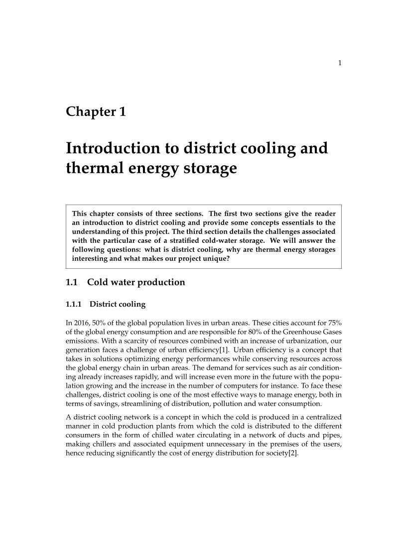
FIGURE 1.1: Representation of a district cooling network
The first district cooling networks were developed on a non-profit basis. Owners ofmultiple buildings (hospitals, university campuses, military camps and airports) in-stalled them with the objective to simplify the operational management of their facili-ties. The first commercial district-cooling network appeared in Hartford, Connecticut(United States) in 1962 when Hartford Steam Company opened the world’s first com-bined heating and cooling system for commercial service[3]. They are numerous ad-vantages for such systems. A centralized facility benefits from more improved analysisand designs than when it comes to small and scattered units, and can handle variationsand different load profiles of consumers much more efficiently. As a result, the produc-tion equipment used in centralized facilities generally present a much higher efficiencythan several smaller units. When particularly strict regulations are in place, you canadd additional equipment to control pollution in much better economic conditions. Butthe improvement are also on the user side: maintenance of production equipment, re-quiring highly trained and qualified staff, no longer ask the consumers’ participation.In centralized systems, maintenance regards a smaller number of equipment and canbe managed by means of computer systems, which represents a reduction of mainte-nance personnel and costs. Finally, it is worth mentioning that district cooling benefitedgreatly of the development of air conditioning in buildings. Air-conditioning has be-come increasingly necessary in many situations, especially in urban centers, which aremost affected by district cooling networks.
The design of a district cooling network requires considering many parameters to en-sure a competitive investment associated with a set combining flexibility, energy effi-ciency, operational savings, capacity and longevity. Amongst these parameters we canhighlight the energy production cost analysis, the requirements of future users, their
1.1. Cold water production 3
demands and load demand, the choice of type and number of cooling installations.Each project is very different and should be studied like a particular case, because eachsituation is unique and the variety of technical solutions encountered and describedbelow will show that it is important not to generalize. Adding a storage medium isan additional way of setting a rational management of district cooling, its design andthe choice of technology for better complementarity with the production system is theresult of a detailed and unique study.
1.1.2 Cooling techniques
Two main industrial cooling techniques exist for chilled water production. The first oneis based on vapor compression, the second is based on absorption. Other techniquesmay however be considered such as free cooling, adsorption chillers, ice slurries sys-tems, gas expansion systems or even deep water source cooling whose good exampleis the cooling network of Fortum Heat and Power (historically started by Birka Energi)in Stockholm which takes advantage of the Baltic Sea waters[4][5]. For simplicity andbecause it is enough for a basic understanding, we will limit our further explanationsto vapor compression systems.
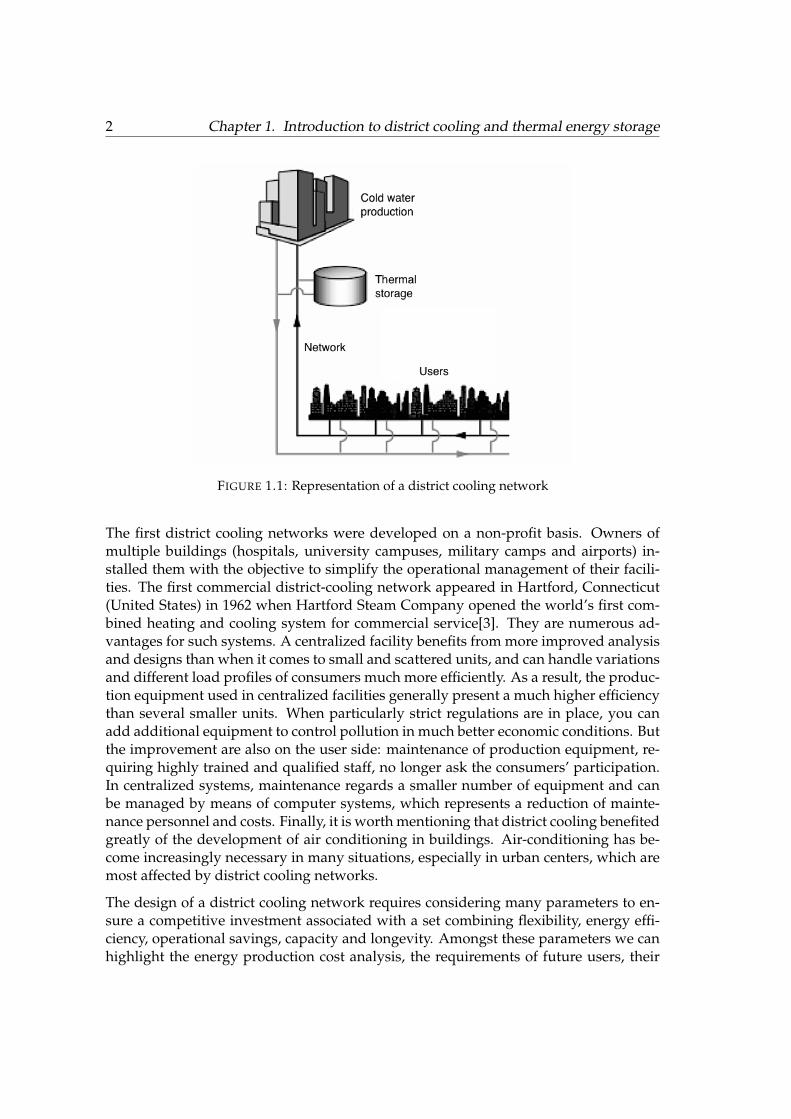
The most common way to produce cold by an industrial process is to use a compressioncycle, in which a fluid is compressed, condensed, expanded and evaporated. The figurebelow illustrates the cold production technique by vapor compression.
FIGURE 1.2: Representation of a vapor compression cycle
A compression cycle can be broken down as follows:
4 Chapter 1. Introduction to district cooling and thermal energy storage
• The refrigerant at low pressure, slightly superheated, is brought to high pressureand high temperature via the compressor;
• After cooling in the condenser, the vapor of the refrigerant fluid is completely con-densed and the heat released by these operations is discharged into the ambientmedium (cooling water or ambient air);
• The condensate is expanded to low pressure and at low temperature through apressure regulator or expansion valve;
• The wet refrigerant stream enters the evaporator and absorbs the heat of the ambi-ent medium (water from the evaporator at a low temperature: 0.5 to 10◦C), whileevaporating and returning to a state of superheated steam.
The efficiency of the chiller is determined by calculating a coefficient of performance(COP), which is defined by the ratio of the cooling energy supplied to the energy con-sumed. With QC the energy getting out of the system at the condenser, QE the energygetting in at the evaporator and W the work of the compressor:
COP =QEW
(1.1)
QC = W +QE (1.2)
1.1.3 Compressors for cold production
Three major types of compressors can be considered when it comes to cold production.The three of them are described in the next paragraphs: reciprocating compressors,screw compressors and centrifugal compressors.
Coolers equipped with a reciprocating compressor are generally used for relativelymodest refrigeration powers (less than 1.5 MW) and have a coefficient of performancelower than other types of coolers, which reduces their presence in the field of districtcooling. This technique is well known and easy to operate. However, they are some re-ciprocating compressors whose refrigeration power can go up to 30 MW and producecooling to cryogenic temperatures. They are very effective, but their investment andmaintenance costs are very high.
1.1. Cold water production 5
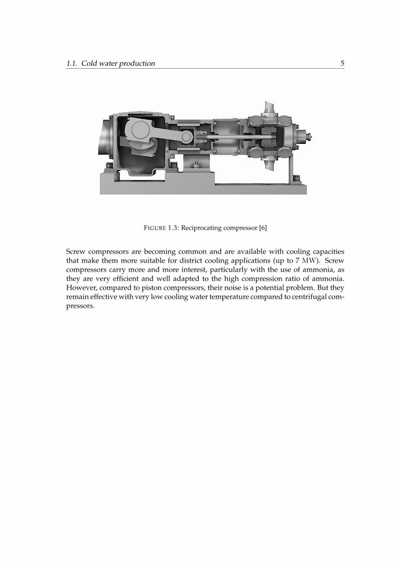
FIGURE 1.3: Reciprocating compressor [6]
Screw compressors are becoming common and are available with cooling capacitiesthat make them more suitable for district cooling applications (up to 7 MW). Screwcompressors carry more and more interest, particularly with the use of ammonia, asthey are very efficient and well adapted to the high compression ratio of ammonia.However, compared to piston compressors, their noise is a potential problem. But theyremain effective with very low cooling water temperature compared to centrifugal com-pressors.

6 Chapter 1. Introduction to district cooling and thermal energy storage
FIGURE 1.4: Screw compressor [7]
Centrifugal compressors are also used in the field of district cooling. Their cooling ca-pacity can be up to 25 MW and they easily adapt to load variations, until a minimumof 40% of maximum load. Below this minimum load instability phenomena are likelyto occur. Reliability, operating cost per megawatt and small dimensions are also greatadvantages. The price difference between the screw compressors and centrifugal com-pressors shall be evaluated on the basis of specific projects.
FIGURE 1.5: Centrifugal compressor [8]
1.2. Cold energy storage 7
1.1.4 Integration of district cooling
Cold-water production is mainly based on the most classical compression systems hav-ing the highest COP. These are usually packaged units and different manufacturershave perfected the technique by combining their experience and modern solutions incomponents such as plate heat exchangers, electronic controls and automation. Themaintenance is well known and spare parts are easily available. A network can haveseveral cooling stations. This means several production plants as well as cold-waterthermal energy storage. This architecture improves the reliability of the distribution. Itcan also become a requirement when the cooling demand exceeds the flow capacity ofthe pipe at the exit of the plant.
Water chillers for district cooling applications require multiple machines to providethe target load. The coolers can be arranged in series, in parallel or a combination ofboth[9]. Connections in series allow different levels of cooling, but the most commontechnique is to have the units in parallel. The cold water at the outlet of the coolers ismixed in a collector before being redirected to the cooling network. But of course, it ispossible to combine the units in series and parallel in order to provide a good operatingflexibility and to adjust the power output to the load.
1.2 Cold energy storage
1.2.1 Advantages and inconveniences
As mentioned previously, thermal energy storage is an attractive strategy for the op-timization of district cooling networks. It generally generates a fairly significant re-duction in investment and operating costs and a more streamlined operation of powergeneration facilities. We often refer to thermal storage (hot or cold) with the abbrevia-tion TES (Thermal Energy Storage). During times when the cooling demand is low, coldproduction facilities operate in excess. The surplus energy produced is stored in a TES.The cold water stored is then used to meet the cooling load demand of customers. Thestorage medium may be chilled water, ice or an eutectic phase change material (morecommon for solar power plant TES).
A cold-water storage presents several advantages:
• It prevents the use of emergency generators in case of mechanical failure of acooling unit;
• Because of the significant variations between the cooling loads during days andnights, it leads to a significant reduction (from 25% to 50%) of the necessary coldproduction power to be installed;
8 Chapter 1. Introduction to district cooling and thermal energy storage
• A cold water storage allows each chiller to operate at its rated power at full capac-ity, also ensuring a more continuous operation with fewer starts and stops, whichimproves both the time-efficiency and life of the machines;
• It allows the shift of electricity use to off-peak hours;
• Throughout the year, cold-water storages improve the average COP of the pro-duction plant because during the night, the condenser temperature is lower thanthe ambient outside temperature during the day.
However they also present some challenges:
• Heat losses in some tanks can sometimes not be negligible, particularly in the caseof small-scale storages. For cold storage of small or medium-scale, heat lossesmay range from 1% to 5% of the storage capacity per day[10];
• Some storage systems can also lead to a decrease in production efficiency. For in-stance, ice slurry storages require a cold production of about -10◦C instead of 5◦Cin normal circumstances: as the COP depends on the temperature of the evapo-rator, the loss of efficiency resulting is about 35% to 40%.
1.2.2 Thermal energy storage
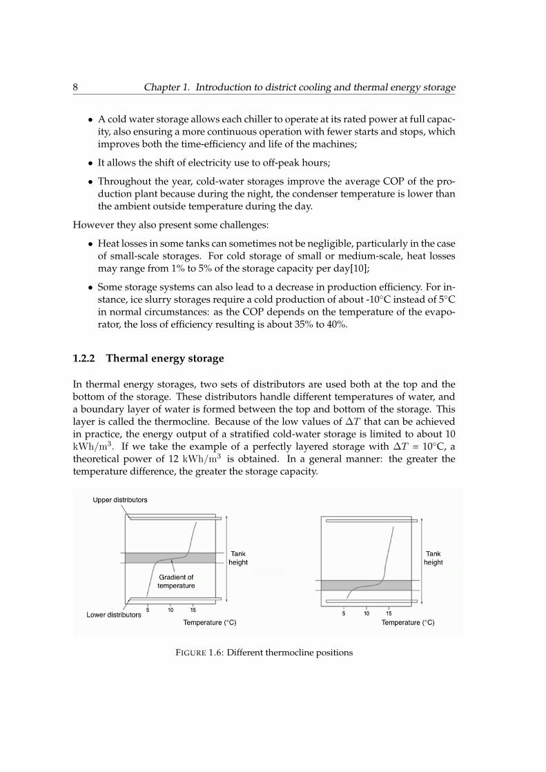
In thermal energy storages, two sets of distributors are used both at the top and thebottom of the storage. These distributors handle different temperatures of water, anda boundary layer of water is formed between the top and bottom of the storage. Thislayer is called the thermocline. Because of the low values of ∆T that can be achievedin practice, the energy output of a stratified cold-water storage is limited to about 10kWh/m3. If we take the example of a perfectly layered storage with ∆T = 10◦C, atheoretical power of 12 kWh/m3 is obtained. In a general manner: the greater thetemperature difference, the greater the storage capacity.
FIGURE 1.6: Different thermocline positions
1.2. Cold energy storage 9
Water does not necessarily have to be the medium, but is the most common one forthe storage of heat or cold. However, to ensure that the water remains in the liquidstate, the value of ∆T may generally not exceed 15◦C for cold storage and 70◦C for heatstorage. It turns out that, unlike hot water storages, cold-water storages are often verylarge. While the hot water storage is the only type of storage used for district heatingnetwork, a large number of cold storage methods have been developed to improve theperformance of district-cooling networks. We could quote diaphragm tanks, labyrinthsystems and baffled tanks amongst others. The one we are interested in is: naturalstratification in stratified cold-water storages.
1.2.3 Natural stratification
Natural stratification systems are probably the most economical and reliable, due totheir simplicity. Gravity separates the cold water (heavier) from the warm water (lighter).Natural stratification tanks ensure efficient separation without the need of physical bar-riers or complex systems of pipes and valves, as in the case of a multiple tank systemwith a large number of tanks. Research projects comparing the efficiency of stratifica-tion systems to other systems such as diaphragms systems, showed that the differencein efficiency is often very low; in many cases the stratification systems, more economi-cal, are preferable.
However, it is important to avoid the damaging or destruction of the thermocline thatcould result from improper design of feed-in and outputs of water. It is hence necessaryto use improved distributors to gently fill the storage with a flow regime allowing a nicethermocline formation, as show is the picture in the previous paragraph. Because of thevery large response time, much attention should be given to transitional operations sothat they do not ruin the stratification.
1.2.4 Categories
Regarding district cooling, we can classify TES in two categories: centralized and dis-tributed energy storages. Centralized TES are located near the central cooling plant,allowing significant economies and the use of ice as well as cold water systems. Dis-tributed TES are located away from the center. They bring improved capacity to bothcold production and pipes level. Thus, TES are used more and more in order to go be-yond the original boundaries of the distribution system capacity. It is a good solutionwhen a more economical operation is required.
We can separate these storages in two other categories: partial storages and total stor-ages. Storages designed to cope with the maximum load of a district-cooling networkare functioning in total storage mode. Those designed to cope with instantaneous loadsoperate in partial storage mode. Partial storage systems use a smaller TES, and theircooling capacities are less important than in the case of a total storage system, whichreduces the initial costs but limits the potential for demand reduction.
10 Chapter 1. Introduction to district cooling and thermal energy storage
Partial storage systems can be divided as well into two categories: peak reduction andpeak shaving systems. The peak reduction method is an intermediate solution betweenthe total storage and peak shaving. The savings generated by peak reduction systemsare higher than in a peak shaving system, and less than for a total load substitution sys-tem. Peak shaving systems are designed to generate maximum savings on cooling plantcapacity: the cooling equipment continuously operates at full load and full capacity 24hours per day.
Centralized TES are usually cheaper due to distance effects, but distributed TES maybe more economic, particularly when the capacity becomes insufficient for the district-cooling network. Indeed, they relieve the cooling network as well as the cold produc-tion plant.
The cost of electricity, cooling demand profile and economic considerations are keyfactors to determine the best duration of charge/discharge cycle. Depending on theratio between the capacity of the TES and the cooling power, we can classify a TESfrom its average cycle time: short-term storage (a few hours or even less), daily storage(charge-discharge cycle of 24h), weekly storage or even seasonal storage. The ratioof storage costs and storage capacity is generally a decreasing function of the storagecapacity, particularly in the case of large water storage systems. As a result, the biggerthe storage is, the longer the optimal cycle time becomes.
Daily storages are the most commonly used and the ones we are interested in. However,a model is needed to determine the optimum storage capacity. Indeed, a large numberof parameters must be taken into account, amongst which we find:
• Load profile;
• Electricity prices depending on the period;
• Cost of the TES;
• ∆T of the TES;
• Thermocline thickness;
• Chiller efficiency depending on the storage temperature.
1.3 Challenges associated
1.3.1 Construction
Tanks for TES are usually made of steel, concrete, fiberglass or plastic. There are dif-ferent types of steel tanks. Large tanks, whose capacity is greater than 1500 m3, areassembled on site from welded steel plates. Smaller tanks (less than 100 m3) may bemade from galvanized steel plates and a reinforcing frame. Pressurized cylindricaltanks are generally used for volumes from 10 to 200 m3 [10]. Underground storage
1.3. Challenges associated 11
allows use of the spared area at the surface to create a car park, a stadium or a parkfor example. Underground storage should only be considered after taking into accountvarious factors:
• Complexity of the pipes of an underground reservoir;
• Impact on the ground and groundwater;
• Regulations on tanks burial (which get tighter and tighter);
• Total investment cost, often twice as large as in the case of an air tank.
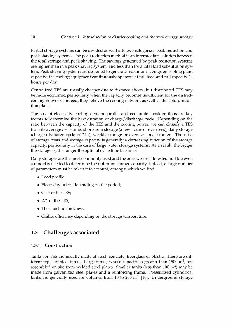
There is another possibility: using existing underground caves. Stockholm and its sur-roundings present caverns that used to be oil storages. Those caves are a great op-portunity to use as stratified cold-water storages; using existing natural infrastructurewould greatly reduce investments costs. There is however, one major complication. Tofacilitate the formation and evolution of a thermocline in a stratified cold-water stor-age, its height should be longer than its width. Indeed, this design choice restricts thecontact areas between warm and cold water. The cave we are considering in this projectpresents the following dimensions:
• 150 m long
• 15 m wide
• 14 m in height
FIGURE 1.7: Dimensions of the cave
In common cold-water storages, the flow entering the tank is usually fully turbulent[11],but the chosen dimensions of the height and width of the tank still lead to relaminar-ization of the flow, and ultimately to the formation and conservation of a thermocline.With a cave of 15 m high and 135 m long, relaminarization is not an easy process toachieve. Several criteria appear to be necessary to relaminarization:
12 Chapter 1. Introduction to district cooling and thermal energy storage
• Uniform flow distribution: the fluid must be injected and removed from the stor-age in a uniform manner, so that we can achieve a horizontal thermocline. In ourcase, several perforated pipes are placed on the top of the cave and some otherperforated pipes on the bottom. Only one side of the tubes serves as inlet, theother side being obstructed. The pressure variations between the inlet and theend of the distributors can lead to non-uniform flow distributions;
• Laminar or transition flow regime: because of the very unusual dimensions of thecave, the flow out of the distributors should be laminar or at least in the laminar-turbulent transition regime, so that we minimize the turbulences as much as pos-sible, hence setting better conditions for a thermocline formation and conserva-tion in time. Far from the thermocline however, small turbulences may not be toomuch of a problem.
As we can see in the above sketch, the length of the storage is not the only obstacle tothe development of a satisfying thermocline. A ramp of approximately 8 m in heightand 5 m wide runs along half of the entire length of the cave. However the velocitiesinvolved for the thermocline (around five millimeters per minute maximum) indicatethat this ramp will probably not be a problem.
1.3.2 Special design
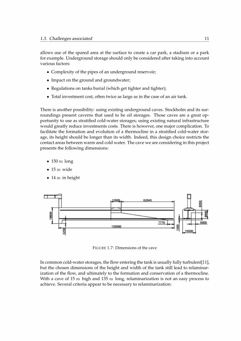
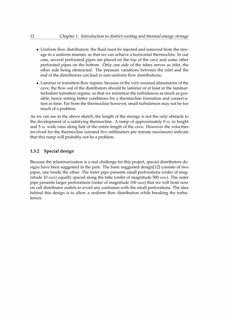
Because the relaminarization is a real challenge for this project, special distributors de-signs have been suggested in the past. The basic suggested design[12] consists of twopipes, one inside the other. The inner pipe presents small perforations (order of mag-nitude 10 mm) equally spaced along the tube (order of magnitude 500 mm). The outerpipe presents larger perforations (order of magnitude 100 mm) that we will from nowon call distributor outlets to avoid any confusion with the small perforations. The ideabehind this design is to allow a uniform flow distribution while breaking the turbu-lences.
1.3. Challenges associated 13
FIGURE 1.8: Cross section of the distributor
FIGURE 1.9: Illustration of the distributor
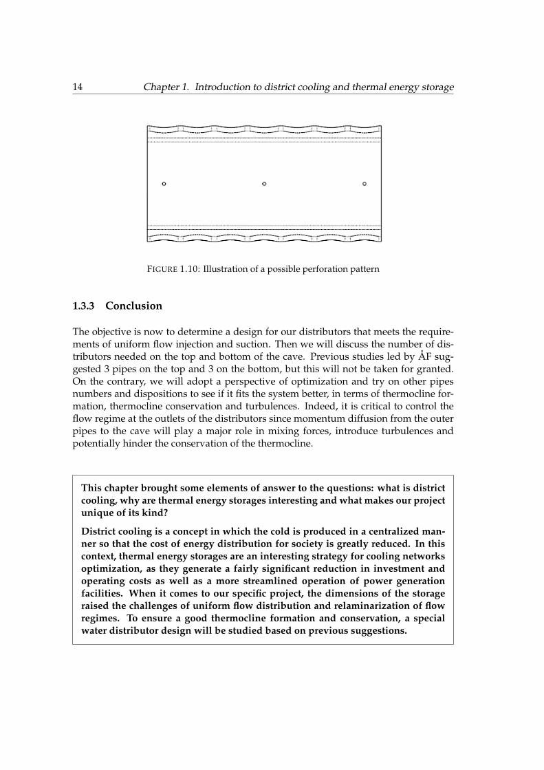
For construction and part assembly purposes, we need an even number of holes in theouter tube for each perforation in the pressure pipe. The perforations must follow apattern: spacing the outlets by 130 mm compels perforations’ spacings to be multiplesof 130 mm.
14 Chapter 1. Introduction to district cooling and thermal energy storage
FIGURE 1.10: Illustration of a possible perforation pattern
1.3.3 Conclusion
The objective is now to determine a design for our distributors that meets the require-ments of uniform flow injection and suction. Then we will discuss the number of dis-tributors needed on the top and bottom of the cave. Previous studies led by ÅF sug-gested 3 pipes on the top and 3 on the bottom, but this will not be taken for granted.On the contrary, we will adopt a perspective of optimization and try on other pipesnumbers and dispositions to see if it fits the system better, in terms of thermocline for-mation, thermocline conservation and turbulences. Indeed, it is critical to control theflow regime at the outlets of the distributors since momentum diffusion from the outerpipes to the cave will play a major role in mixing forces, introduce turbulences andpotentially hinder the conservation of the thermocline.
This chapter brought some elements of answer to the questions: what is districtcooling, why are thermal energy storages interesting and what makes our projectunique of its kind?
District cooling is a concept in which the cold is produced in a centralized man-ner so that the cost of energy distribution for society is greatly reduced. In thiscontext, thermal energy storages are an interesting strategy for cooling networksoptimization, as they generate a fairly significant reduction in investment andoperating costs as well as a more streamlined operation of power generationfacilities. When it comes to our specific project, the dimensions of the storageraised the challenges of uniform flow distribution and relaminarization of flowregimes. To ensure a good thermocline formation and conservation, a specialwater distributor design will be studied based on previous suggestions.
15
Chapter 2
Computational fluid dynamicsconsiderations
This chapter presents three sections. The first section introduces the differentflow regimes and fluid mechanisms happening in the stratified cold-water stor-age. The second section gives basic considerations on computational fluid dy-namics relevant for this project. The third section explains more about conver-gence criteria of numerical simulations. We will answer the following questions:what are the challenges that come with the numerical simulation of a stratifiedcold water storage, what important models will be used and what guaranties theadequacy of the results?
2.1 Fluid mechanics in the Stratified Cold Water Storage
2.1.1 Introduction to transport mechanisms
For our stratified cold-water storage, different areas of the system will present differentflow regimes that are likely to change depending on several factors: storage charging ordischarging, flow rate evolution, thermocline formation, thermocline in motion, etc. Asmentioned in the previous chapter, momentum diffusion at the outlet holes in the outerpipes will play a key role in mixing the fluid, introduce turbulences and potentiallyhinder the formation and conservation of a thermocline. Indeed, turbulent diffusionincreases momentum diffusion as well as energy diffusion; this means more thermalmixing which in terms means a thicker thermocline. Convection heat transfer is also animportant mechanism in the storage when re-injecting warm water after a complete fill-ing with cold-water (may be necessary as a purge to get rid of the stagnant warm wateron the top of the upper-distributors for instance). Conduction heat transfer will alsooccur, especially at the thermocline level where we will find the strongest temperaturegradient. These mechanisms influence greatly the stratification process.
16 Chapter 2. Computational fluid dynamics considerations
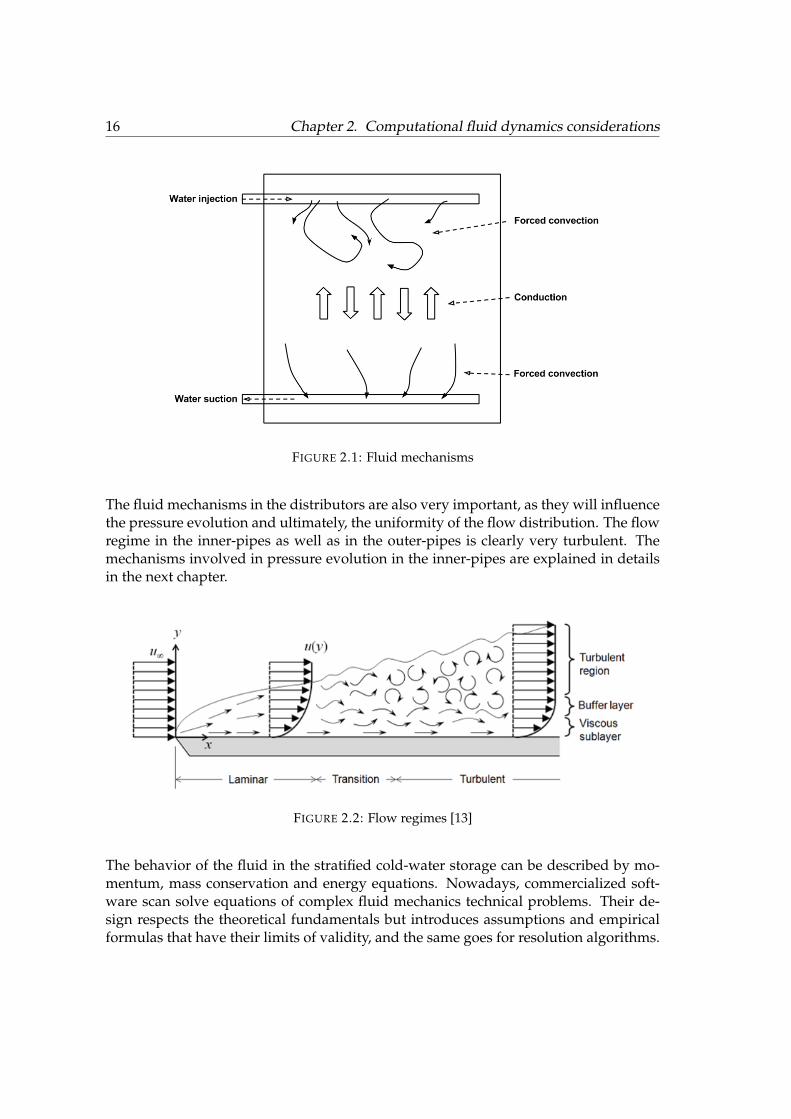
FIGURE 2.1: Fluid mechanisms
The fluid mechanisms in the distributors are also very important, as they will influencethe pressure evolution and ultimately, the uniformity of the flow distribution. The flowregime in the inner-pipes as well as in the outer-pipes is clearly very turbulent. Themechanisms involved in pressure evolution in the inner-pipes are explained in detailsin the next chapter.
FIGURE 2.2: Flow regimes [13]
The behavior of the fluid in the stratified cold-water storage can be described by mo-mentum, mass conservation and energy equations. Nowadays, commercialized soft-ware scan solve equations of complex fluid mechanics technical problems. Their de-sign respects the theoretical fundamentals but introduces assumptions and empiricalformulas that have their limits of validity, and the same goes for resolution algorithms.
2.1. Fluid mechanics in the Stratified Cold Water Storage 17
Using these numerical tools requires the highest vigilance even for fluid mechanics spe-cialists. This project has been conducted with ANSYS 15.0 Fluent.
2.1.2 Dimensionless numbers
Usual fluid mechanics dimensionless numbers can describe the stratification process:the Reynolds number, the Peclet number and the Richardson number[14]. Experimen-tal results shows that, for the same fluid circulating in a given material environment,the flow is laminar at low speeds and becomes turbulent for high speeds. The transitionfrom one to the other depends on the relative importance of inertia forces and viscosityforces. The ratio of these forces, which appear in the Navier Stokes equation, leads to adimensionless number called the Reynolds number:
Re =V d
ν(2.1)
Here we have ν the kinematic viscosity of the fluid, V the average velocity of the fluid,d the characteristic dimension of the flow. Before Re ' 2000 the flow is laminar, thenthe flow becomes turbulent. The number 2000 is an approximation, and between thelaminar and turbulent regimes we observe a transition region. The Reynolds numberclose to the outlets of the outer pipes should be as low as possible. The Peclet numberrepresents the relative strength of convection and diffusion forces. For a flow governedby pure diffusion, the Peclet number is close to 0. For a flow where convection takesover, the Peclet number reaches infinity. With α being the thermal conductivity, thePeclet number is defined as:
Pe =V d
α(2.2)
The Peclet number in the thermocline should be as low as possible since we wish tolimit the convection forces. Finally, the Richardson number relates the ratio betweenthe gravitational potential energy of a fluid particle and its kinetic energy. To put itsimply, this number is the ratio of the buoyancy forces and the mixing forces, or naturalconvection and forced convection. It generally takes values between 0 and 10 and aRichardson number smaller than 1 indicates a flow governed by forced convection. Thegravity is called g and the characteristic length is d. With β being the thermal expansioncoefficient of the fluid and ∆T the temperature difference of the fluid considered:
Ri =gβ∆Td
v2(2.3)
In the last chapter, some of these dimensionless numbers and more will be investi-gated.
18 Chapter 2. Computational fluid dynamics considerations
2.2 CFD models
2.2.1 Turbulence modeling
Numerical simulations require to choose different fluid mechanics models. To under-stand the choices that have been made between these models, it is important to receivea short but proper introduction to the basics of turbulences.
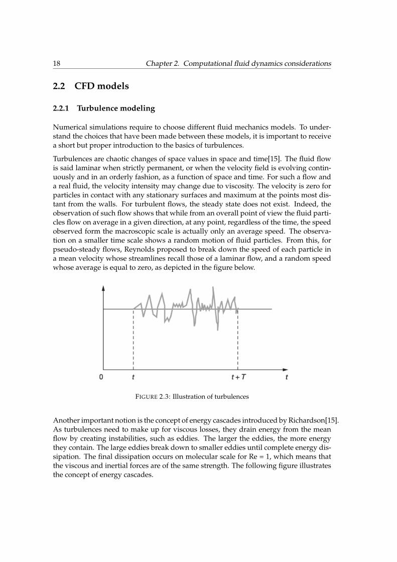
Turbulences are chaotic changes of space values in space and time[15]. The fluid flowis said laminar when strictly permanent, or when the velocity field is evolving contin-uously and in an orderly fashion, as a function of space and time. For such a flow anda real fluid, the velocity intensity may change due to viscosity. The velocity is zero forparticles in contact with any stationary surfaces and maximum at the points most dis-tant from the walls. For turbulent flows, the steady state does not exist. Indeed, theobservation of such flow shows that while from an overall point of view the fluid parti-cles flow on average in a given direction, at any point, regardless of the time, the speedobserved form the macroscopic scale is actually only an average speed. The observa-tion on a smaller time scale shows a random motion of fluid particles. From this, forpseudo-steady flows, Reynolds proposed to break down the speed of each particle ina mean velocity whose streamlines recall those of a laminar flow, and a random speedwhose average is equal to zero, as depicted in the figure below.
FIGURE 2.3: Illustration of turbulences
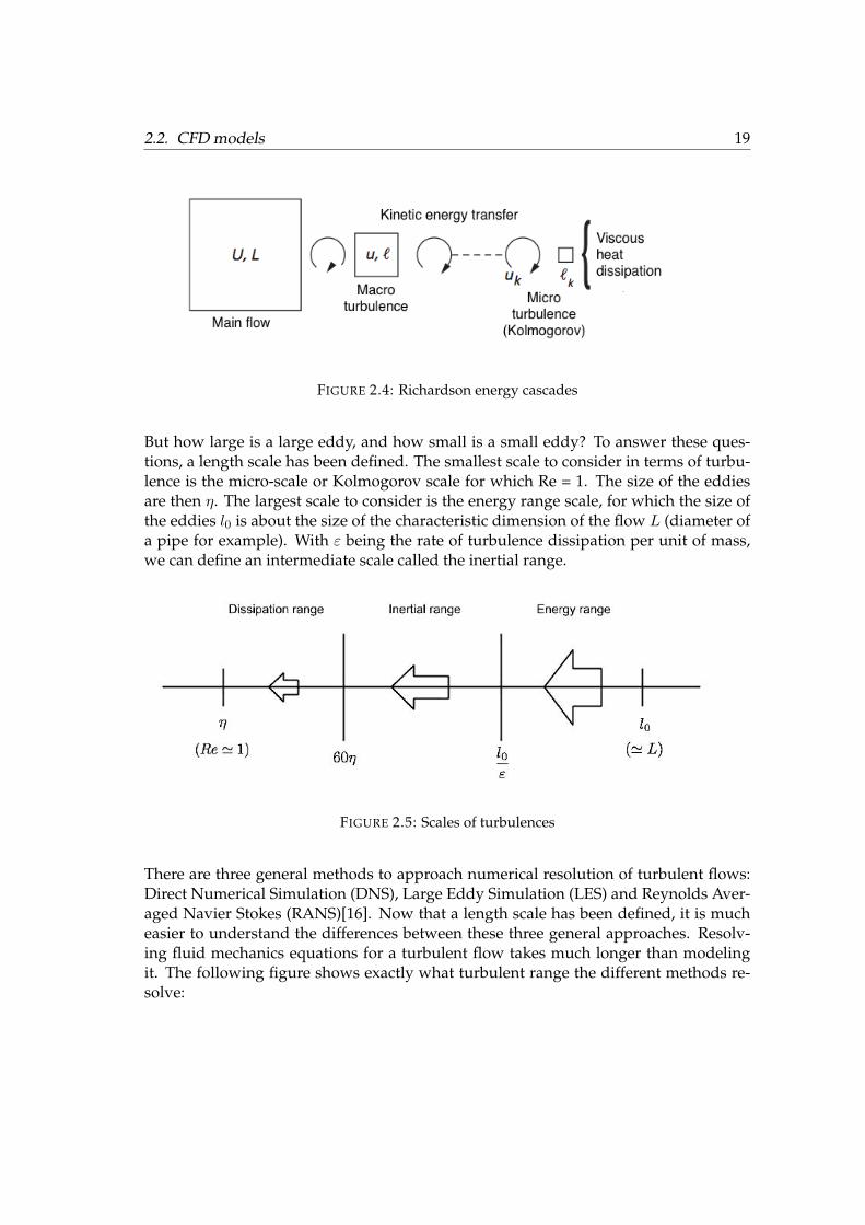
Another important notion is the concept of energy cascades introduced by Richardson[15].As turbulences need to make up for viscous losses, they drain energy from the meanflow by creating instabilities, such as eddies. The larger the eddies, the more energythey contain. The large eddies break down to smaller eddies until complete energy dis-sipation. The final dissipation occurs on molecular scale for Re = 1, which means thatthe viscous and inertial forces are of the same strength. The following figure illustratesthe concept of energy cascades.
2.2. CFD models 19
FIGURE 2.4: Richardson energy cascades
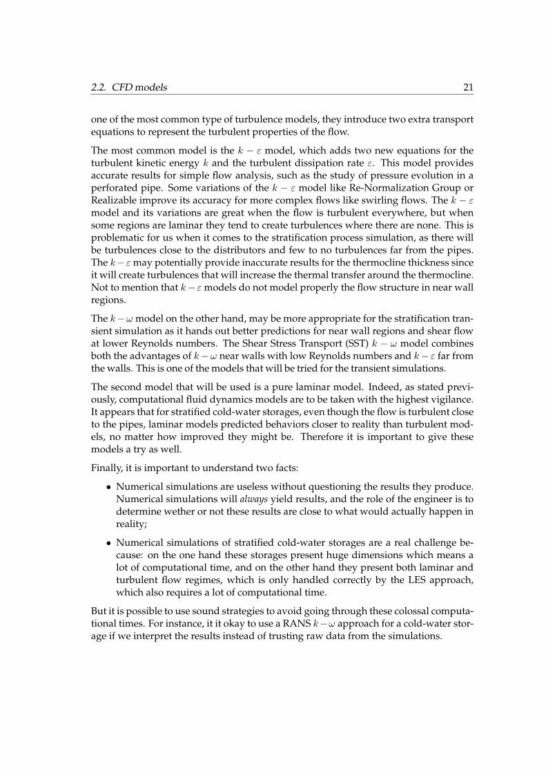
But how large is a large eddy, and how small is a small eddy? To answer these ques-tions, a length scale has been defined. The smallest scale to consider in terms of turbu-lence is the micro-scale or Kolmogorov scale for which Re = 1. The size of the eddiesare then η. The largest scale to consider is the energy range scale, for which the size ofthe eddies l0 is about the size of the characteristic dimension of the flow L (diameter ofa pipe for example). With ε being the rate of turbulence dissipation per unit of mass,we can define an intermediate scale called the inertial range.
FIGURE 2.5: Scales of turbulences
There are three general methods to approach numerical resolution of turbulent flows:Direct Numerical Simulation (DNS), Large Eddy Simulation (LES) and Reynolds Aver-aged Navier Stokes (RANS)[16]. Now that a length scale has been defined, it is mucheasier to understand the differences between these three general approaches. Resolv-ing fluid mechanics equations for a turbulent flow takes much longer than modelingit. The following figure shows exactly what turbulent range the different methods re-solve:

20 Chapter 2. Computational fluid dynamics considerations
FIGURE 2.6: Scales of turbulences and their numerical resolution
Direct Numerical Simulation is very time consuming and is generally used for researchto understand fluid mechanisms at the molecular level. With the improvement of com-puting power, Large Eddy Simulations are used more and more in the industry, for finaldesigns or when the problem requires the resolution of large eddies. The Reynolds-Averaged Navier Stokes is the one mostly used in the industry, because of its goodratio calculation time to quality of results. This project will be conducted with RANSapproach.
2.2.2 Reynolds Averaged Navier Stockes
In the RANS approach, eddies are not solved but modeled. Transport equations aretime-averaged, so that the turbulences are accounted for in a statistical manner. Whenthe Navier Stokes equations (momentum equations) are time-averaged, a new quantityappears: the Reynolds stresses quantity. The difference between the RANS models liesin how this new quantity is defined. Finally, the number of new equations they in-troduce classifies them: one equation turbulence models solve one turbulent transportequation, usually the turbulent kinetic energy, and two equation turbulence models are
2.2. CFD models 21
one of the most common type of turbulence models, they introduce two extra transportequations to represent the turbulent properties of the flow.
The most common model is the k − ε model, which adds two new equations for theturbulent kinetic energy k and the turbulent dissipation rate ε. This model providesaccurate results for simple flow analysis, such as the study of pressure evolution in aperforated pipe. Some variations of the k − ε model like Re-Normalization Group orRealizable improve its accuracy for more complex flows like swirling flows. The k − εmodel and its variations are great when the flow is turbulent everywhere, but whensome regions are laminar they tend to create turbulences where there are none. This isproblematic for us when it comes to the stratification process simulation, as there willbe turbulences close to the distributors and few to no turbulences far from the pipes.The k−ε may potentially provide inaccurate results for the thermocline thickness sinceit will create turbulences that will increase the thermal transfer around the thermocline.Not to mention that k− ε models do not model properly the flow structure in near wallregions.
The k−ω model on the other hand, may be more appropriate for the stratification tran-sient simulation as it hands out better predictions for near wall regions and shear flowat lower Reynolds numbers. The Shear Stress Transport (SST) k − ω model combinesboth the advantages of k−ω near walls with low Reynolds numbers and k− ε far fromthe walls. This is one of the models that will be tried for the transient simulations.
The second model that will be used is a pure laminar model. Indeed, as stated previ-ously, computational fluid dynamics models are to be taken with the highest vigilance.It appears that for stratified cold-water storages, even though the flow is turbulent closeto the pipes, laminar models predicted behaviors closer to reality than turbulent mod-els, no matter how improved they might be. Therefore it is important to give thesemodels a try as well.
Finally, it is important to understand two facts:
• Numerical simulations are useless without questioning the results they produce.Numerical simulations will always yield results, and the role of the engineer is todetermine wether or not these results are close to what would actually happen inreality;
• Numerical simulations of stratified cold-water storages are a real challenge be-cause: on the one hand these storages present huge dimensions which means alot of computational time, and on the other hand they present both laminar andturbulent flow regimes, which is only handled correctly by the LES approach,which also requires a lot of computational time.
But it is possible to use sound strategies to avoid going through these colossal computa-tional times. For instance, it it okay to use a RANS k−ω approach for a cold-water stor-age if we interpret the results instead of trusting raw data from the simulations.
22 Chapter 2. Computational fluid dynamics considerations
2.2.3 Wall treatment and wall fonctions
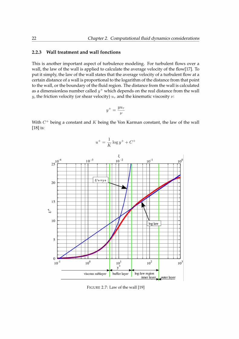
This is another important aspect of turbulence modeling. For turbulent flows over awall, the law of the wall is applied to calculate the average velocity of the flow[17]. Toput it simply, the law of the wall states that the average velocity of a turbulent flow at acertain distance of a wall is proportional to the logarithm of the distance from that pointto the wall, or the boundary of the fluid region. The distance from the wall is calculatedas a dimensionless number called y+ which depends on the real distance from the wally, the friction velocity (or shear velocity) uτ and the kinematic viscosity ν:
y+ =yuτν
With C+ being a constant and K being the Von Karman constant, the law of the wall[18] is:
u+ =1
Klog y+ + C+
FIGURE 2.7: Law of the wall [19]

2.3. Convergence criteria 23
Below the region where the law of the wall is applicable, that is to say the buffer layerand viscous sublayer, there are other estimations for friction velocity. In the viscoussublayer, for y+<5 the dimensionless velocity u+ of the turbulent flow is equal to y+.In the buffer layer, no law applies. This concept is important when choosing the size ofthe first mesh close to the walls. After y+ ' 11 the log law is more accurate than thelinear approximation y+ = u+.
When using wall functions and for most models, Fluent connects the viscosity-affectedregion to the fully turbulent region with the laws introduced before, and no cells shouldexist in the viscous sublayer. That means that the first cell should be at least at y+ = 11.If one wants to resolve the viscous sublayer, y+ = 1 is required. However, in the case ofthe improved SST k − ω models, any cell size works. It is also possible to use scalablewall functions that will ignore the mesh below y+ = 11.
2.2.4 Buoyancy modeling
The temperature difference in the stratified cold-water storage leads to a buoyancy-driven flow. The classical approach to modeling buoyancy is the Boussinesq modelwhich considers a constant density in every equation except for the buoyancy term ofthe momentum equations. This approach gives acceptable results when the tempera-ture difference (and so the density difference) is small.
For the transient simulations, we will use the Boussinesq approximation, as it will sim-plify the problem and save computational time. Firstly, the literature seems very un-clear about what temperature is or isn’t acceptable to apply the Boussinesq approxima-tion. One criterion recommended by Fluent[20] is β∆T � 1. At 10◦C the volumetricthermal expansion coefficient of water is β = 8.8 × 10⁻⁵K−1 and our temperature dif-ference in the storage is 10◦C, which yields the following result:
β∆T = 8.8× 10−5 × 10 = 8.8× 10⁻⁴ � 1 (2.4)
We will then use the Boussinesq approximation.
2.3 Convergence criteria
Convergence is a very large topic and remains often a very unclear area. When dealingwith convergence and residuals monitoring, it is important to ask ourselves the rightquestions. The following subsections gives key elements that have been used to handleconvergence in this master thesis. This gathering of information is the result of anintensive research on CFD online forums, topic "Fluent".
24 Chapter 2. Computational fluid dynamics considerations
2.3.1 Residuals and numerical errors
When convergence is reached, different conditions should be satisfied. First of all, eitherdiscrete conservation equations (momentum and energy equations) should be obeyedin every cell to a specified tolerance which is defined by the size of the residuals orthe solution should no longer changes with subsequent iterations, e.g. the residuals donot change anymore. We then understand the importance of monitoring convergenceusing residual history. It seems generally agreed that a decrease in residuals by threeorders of magnitude indicates a qualitative convergence. At the very least, the majorflow features should at this point be established, and it is in many cases enough for theresults we may need. However, we also encounter engineers writing that scaled energyresidual should decrease to at least 10−6 when using the pressure-based solver, andscaled species residual may need to decrease to 10−5 to achieve species balance.
This is about ensuring that overall mass, momentum, energy, and scalar balances areachieved. But it is also possible to monitor quantitative convergence of the simulationby monitoring other relevant key variables/physical quantities for a confirmation ofthe results. In our case, the pressure along the inner pipes of the distributors can bemonitored to keep an eye on the simulation evolution; when convergence is reached,the pressure characteristic should no longer change.
Numerical errors are associated with calculation of cell gradients and cell face interpo-lations.
Concerning numerical errors, here are some ideas to limit them:
• Using higher-order discretization schemes (such as second-order upwind)
• Attempting to align the grid with the flow to minimize false diffusion
• Refining the mesh
• Minimizing variations in cell size in non-uniform meshes
• Improving the uniformity of the mesh to limit truncation errors
• Using FLUENT ability to adapt the mesh based on cell size variation
• Minimizing cell skewness and aspect ratio
• Avoid aspect ratios higher than 5:1
• Optimal quad/hex cells should be bounded angles of 90 degrees
• Optimal tri/tet cells should be equilateral
2.3. Convergence criteria 25
2.3.2 Heat/mass conservation and grid independence
At convergence one should also make sure that overall mass, heat and species conser-vation is satisfied. The net flux imbalance should be less than 1% of the smallest fluxthrough the domain boundary.
The size of the mesh can impact the final solution. We say that a grid-independentsolution exists when the solution no longer changes after a mesh refinement. The pro-cedure to follow is quite systematic: generate a new and finer mesh, start calculationsuntil convergence, compare the results obtained for the different sizes mesh, repeat theprocedure if necessary. In this project, we adopted the following criterion: a solution isgrid-independent when a mesh refinement of 15% leads to a solution change less that5%.
2.3.3 Accelerating convergence
Convergence can be accelerated by several factors. The first one is supplying betterinitial conditions or starting from a previous solution. If the convergence is still hard toachieve, one could try to gradually increase under-relaxation factors or Courant num-ber: doing that, convergence is preferred over time-cost, which means that the simula-tion might find its way to convergence but it will take a longer amount of time. How-ever it is often recommended not to play with under-relaxation factors when the simu-lation does not present combustions or phase change. One can also control the Multi-Grid solver settings, which is also generally not recommended for non-experiencedCFD analysts.
If after everything, the flow features do not seem reasonable (as we said before, resultshave to be interpreted), then one might reconsider the physical models and boundaryconditions of the simulation. Also, examining mesh quality and sometimes remeshingthe system can help. Inadequate choice of domain and boundary locations (especiallythe outlet boundary) can significantly impact the solution accuracy and convergence.Some pairs of inlets/outlets seem to not work well together, also it is preferable to avoidthe pair mass flow inlet/pressure outlet and use velocity inlet/pressure outlet instead.The reason why these pair problems appear are inherent to the way Fluent is coded,and is not explained by the notice.
This chapter brought some elements of answer to the questions: what are thechallenges that come with the numerical simulation of a stratified cold-waterstorage, what important models will be used and what guaranties the adequacyof the results?
Stratified cold-water storages present both laminar and turbulent flows, whichput as a pair are not well handled by today’s commercialized softwares. If Large
26 Chapter 2. Computational fluid dynamics considerations
Eddy Simulations would be the way-to-go here, the outsized differences in or-ders of magnitudes when it comes to fluid mechanisms would require a very finemesh over the entire storage and lead to astronomical computational times. Thenecessary simplifications will be conducted and we will keep a critical eye on theresults. Reynolds Averaged Navier-Stokes models will be used, and the Boussi-nesq approximation will serve for the transient simulations. The adequacy ofthe results is guarantied by controlling a multitude of factors to reduce numeri-cal errors, verify heat/mass conservation, grid independence and ensure conver-gence.
27
Chapter 3
Distributor design: theory
This chapter consists of three sections. The first section reminds the fundamen-tals of perforated distributors theory. The second section details the derivationof formula for pressure evolutions in the distributor. The third section defines adesign criterion for good flow distribution. We will answer the following ques-tions: what is the mathematical expression of the pressure evolution in the innerpipes of the distributors and what design will be the starting point of the numer-ical simulations?
3.1 Perforated distributor theory
3.1.1 Importance of a pre-study
One of the objectives of a numerical simulation is to verify the behavior of a systemunder different operating conditions and improve its design. Simulations can be verytime intensive, therefore before running a CFD simulation, it is important to have anidea of the final design we would like. Trying uncritically to find a suitable designby running different CFD simulations with different designs would be both time con-suming and inefficient. To obtain an optimum flow distribution, it is essential to giveproper consideration to flow conditions upstream and downstream in the distributor,flow behavior in the distributor, and distribution requirements.
In this chapter, we will go through the fundamentals of perforated distributors theory,derive formula for pressure evolutions in the distributors, define a design criterion forgood flow distribution and finally apply this criterion to our case.
3.1.2 Basic theory
Consider a simple horizontal perforated tube, opened on the left side and closed on theright side. The pressure variations inside the tube come from frictional pressure dropalong the length of the pipe and pressure recovery due to kinetic energy or momentumchanges. The physical principles behind these pressure variations will be explained in
28 Chapter 3. Distributor design: theory
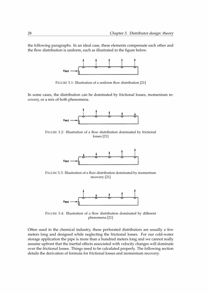
the following paragraphs. In an ideal case, these elements compensate each other andthe flow distribution is uniform, such as illustrated in the figure below.
FIGURE 3.1: Illustration of a uniform flow distribution [21]
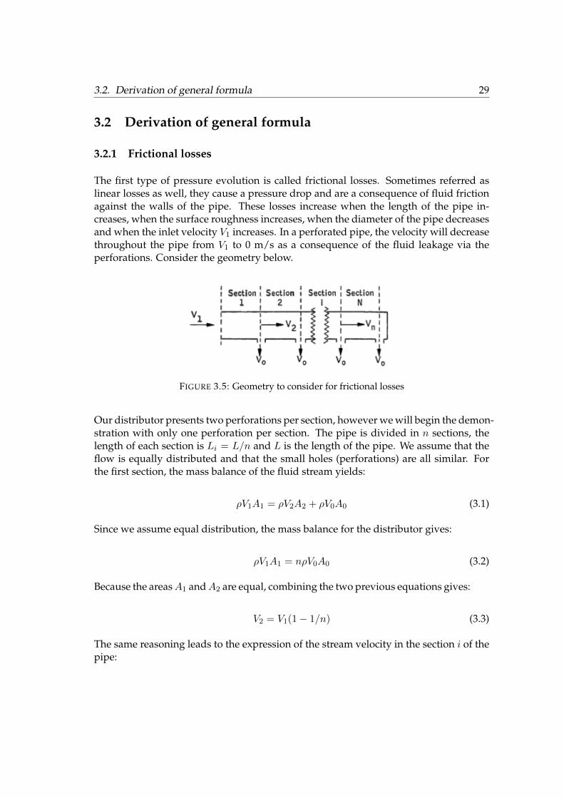
In some cases, the distribution can be dominated by frictional losses, momentum re-covery, or a mix of both phenomena.
FIGURE 3.2: Illustration of a flow distribution dominated by frictionallosses [21]
FIGURE 3.3: Illustration of a flow distribution dominated by momentumrecovery [21]
FIGURE 3.4: Illustration of a flow distribution dominated by differentphenomena [21]
Often used in the chemical industry, these perforated distributors are usually a fewmeters long and designed while neglecting the frictional losses. For our cold-waterstorage application the pipe is more than a hundred meters long and we cannot reallyassume upfront that the inertial effects associated with velocity changes will dominateover the frictional losses. Things need to be calculated properly. The following sectiondetails the derivation of formula for frictional losses and momentum recovery.
3.2. Derivation of general formula 29
3.2 Derivation of general formula
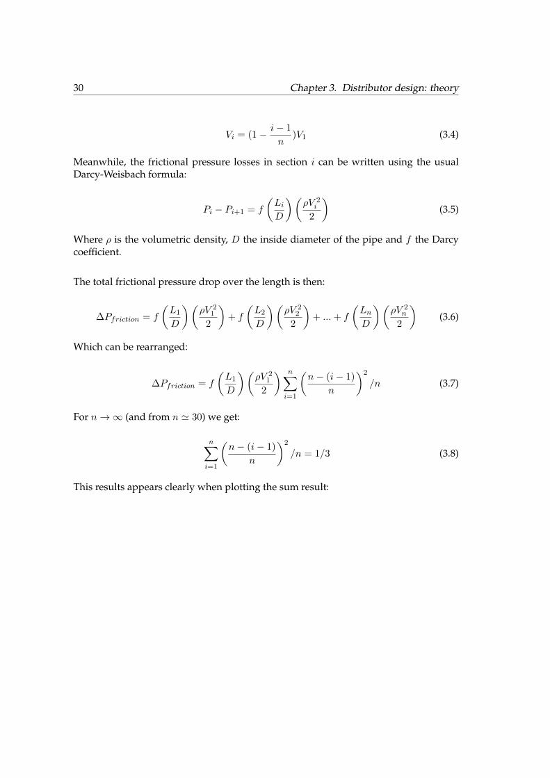
3.2.1 Frictional losses
The first type of pressure evolution is called frictional losses. Sometimes referred aslinear losses as well, they cause a pressure drop and are a consequence of fluid frictionagainst the walls of the pipe. These losses increase when the length of the pipe in-creases, when the surface roughness increases, when the diameter of the pipe decreasesand when the inlet velocity V1 increases. In a perforated pipe, the velocity will decreasethroughout the pipe from V1 to 0 m/s as a consequence of the fluid leakage via theperforations. Consider the geometry below.
FIGURE 3.5: Geometry to consider for frictional losses
Our distributor presents two perforations per section, however we will begin the demon-stration with only one perforation per section. The pipe is divided in n sections, thelength of each section is Li = L/n and L is the length of the pipe. We assume that theflow is equally distributed and that the small holes (perforations) are all similar. Forthe first section, the mass balance of the fluid stream yields:
ρV1A1 = ρV2A2 + ρV0A0 (3.1)
Since we assume equal distribution, the mass balance for the distributor gives:
ρV1A1 = nρV0A0 (3.2)
Because the areasA1 andA2 are equal, combining the two previous equations gives:
V2 = V1(1− 1/n) (3.3)
The same reasoning leads to the expression of the stream velocity in the section i of thepipe:
30 Chapter 3. Distributor design: theory
Vi = (1− i− 1
n)V1 (3.4)
Meanwhile, the frictional pressure losses in section i can be written using the usualDarcy-Weisbach formula:
Pi − Pi+1 = f
(LiD
)(ρV 2
i
2
)(3.5)
Where ρ is the volumetric density, D the inside diameter of the pipe and f the Darcycoefficient.
The total frictional pressure drop over the length is then:
∆Pfriction = f
(L1
D
)(ρV 2
1
2
)+ f
(L2
D
)(ρV 2
2
2
)+ ...+ f
(LnD
)(ρV 2
n
2
)(3.6)
Which can be rearranged:
∆Pfriction = f
(L1
D
)(ρV 2
1
2
) n∑i=1
(n− (i− 1)
n
)2
/n (3.7)
For n→∞ (and from n ' 30) we get:
n∑i=1
(n− (i− 1)
n
)2
/n = 1/3 (3.8)
This results appears clearly when plotting the sum result:
3.2. Derivation of general formula 31
1 10 20 30 40 50
1
0.33
0.67
1
n
∑ni=1
(n−(i−1)
n
)2/n
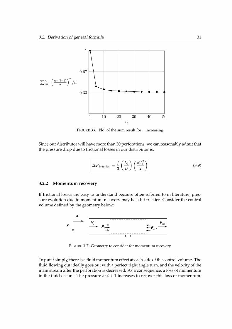
FIGURE 3.6: Plot of the sum result for n increasing
Since our distributor will have more than 30 perforations, we can reasonably admit thatthe pressure drop due to frictional losses in our distributor is:
∆Pfriction =f
3
(L1
D
)(ρV 2
1
2
)(3.9)
3.2.2 Momentum recovery
If frictional losses are easy to understand because often referred to in literature, pres-sure evolution due to momentum recovery may be a bit trickier. Consider the controlvolume defined by the geometry below:
FIGURE 3.7: Geometry to consider for momentum recovery
To put it simply, there is a fluid momentum effect at each side of the control volume. Thefluid flowing out ideally goes out with a perfect right angle turn, and the velocity of themain stream after the perforation is decreased. As a consequence, a loss of momentumin the fluid occurs. The pressure at i + 1 increases to recover this loss of momentum.
32 Chapter 3. Distributor design: theory
Hence the name momentum recovery. For the control volume between sections i andi+ 1 we can write the conservation of momentum on the X axis:
∑F = moutVout −minVin (3.10)
∑F = ρAV 2
i+1 − ρAV 2i (3.11)
The force components are the pressure forces on each section i and i + 1 as well as thepressure forces from the pipe walls to the control volume. We will then neglect the Xcomponent of resistance of the walls FwallX , small compared to the other forces.
∑F = PiA− Pi+1A+ XXXXFwallX (3.12)
The previous equations can be rearranged in a simpler form:
Pi+1 − Pi = ρV 2i − ρV 2
i+1 (3.13)
However, the fluid flowing out by the perforations does not do a perfect right angle. Totake into account the inefficiency of the turn, we introduce the inefficiency coefficientk (which value is between 0 and 1). This coefficient has been determined empiricallyin the past and is known to be around 0.55 for turbulent flows. Finally, we get for theentire distributor:
Pn − P1 = kρ[(V 21 − V 2
2 ) + (V 22 − V 2
3 ) + ...+ (V 2n−1 − V 2
n )] (3.14)
Which simplifies in:
P1 − Pn = −kρV 21 [1− 1/n2] (3.15)
For a large number of perforations, we derive the following:
∆Pmomentum = −kρV 21 (3.16)
Finally, we found what we were looking for. The total pressure evolution in the distrib-utor due to friction and momentum recovery is:
∆Ptotal = ∆Pfriction + ∆Pmomentum =
(fL
3D− 2k
)ρV 2
1
2(3.17)
3.2. Derivation of general formula 33
∆Ptotal =
(fL
3D− 2k
)ρV 2
1
2(3.18)
3.2.3 Two perforations
In this section, we consider a distributor with more than 1 perforation. If the innerpipe presents P perforations per section, the mass balance for the entire distributorbecomes:
ρV1A1 = nPρV0A0 (3.19)
The mass balance for the section 1 becomes:
ρV1A1 = ρV2A2 + PρV0A0 (3.20)
The mass balance for the section i becomes:
ρViAi = ρVi+1Ai+1 + PρV0A0 (3.21)
Once again all the areas are equal, so the previous equations can be combined andrearranged such as:
Vi+1 =
(1− i
n
)V1 (3.22)
Which can also we written:
Vi =
(1− i− 1
n
)V1 (3.23)
From this step, we observe that the definition of Vi does not depend on the numberof perforations per section. From then, we can conduct the same calculations as in theprevious paragraphs and find that the total pressure evolution for a distributor with Pperforations per section is:
∆Ptotal = ∆Pfriction + ∆Pmomentum =
(fL
3D− 2k
)ρV 2
1
2(3.24)
One should keep in mind that this formula is only valid for a perforated distributorthat injects a fluid from the distributor towards the exterior environment (the thermal
34 Chapter 3. Distributor design: theory
storage in our case). If the flow is reversed, so that the distributor is sucking the fluidin, the inefficiency coefficient k becomes negative and the total pressure drop increases.In our case, the pipes will be used both ways.
3.3 Design criterion
3.3.1 Good flow distribution
For a good flow distribution, we can read in the literature that the average pressuredrop ∆P0 across the small holes must be one order of magnitude superior to the totalpressure drop ∆Ptotal throughout the pipe (that we just calculated in the previous sec-tion). This statement feels right. Indeed if the relative pressure drop variation is lowbetween all the small holes, the variation in flow will be small too.
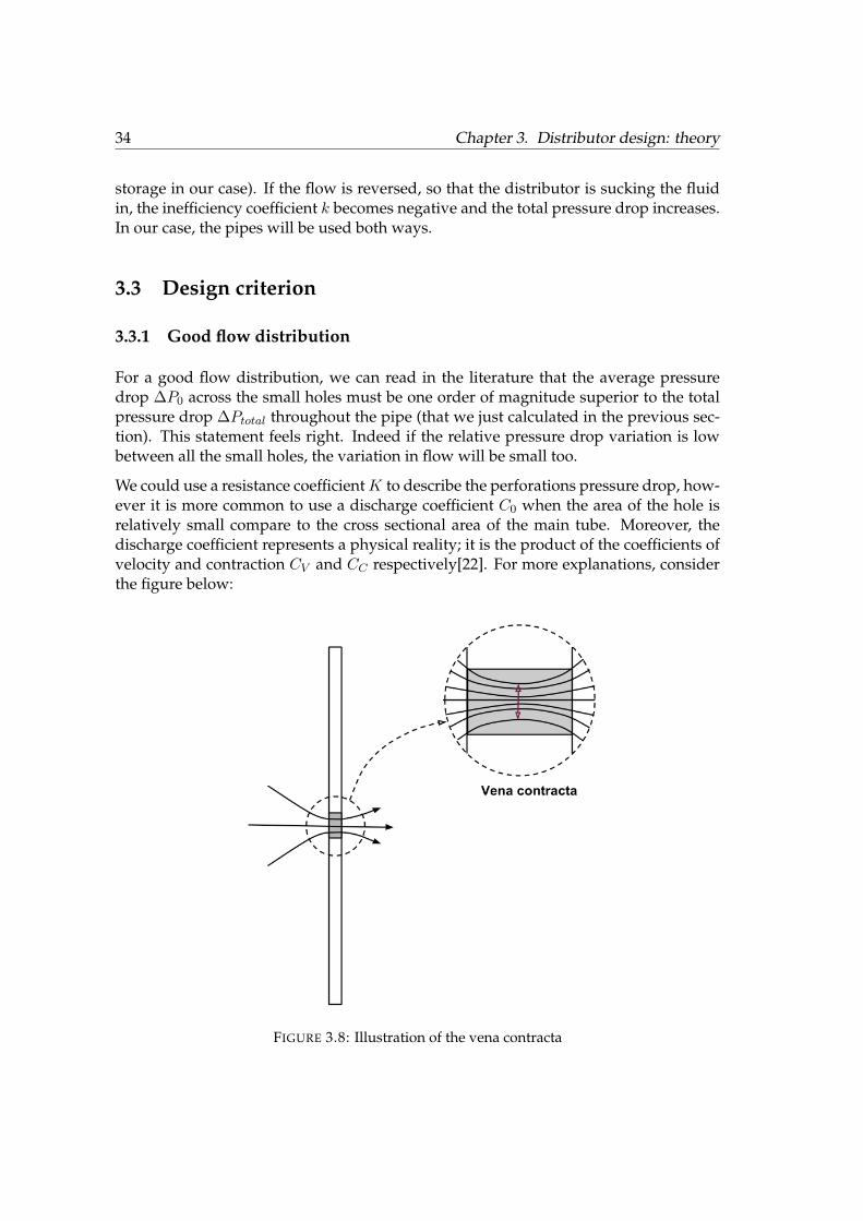
We could use a resistance coefficientK to describe the perforations pressure drop, how-ever it is more common to use a discharge coefficient C0 when the area of the hole isrelatively small compare to the cross sectional area of the main tube. Moreover, thedischarge coefficient represents a physical reality; it is the product of the coefficients ofvelocity and contraction CV and CC respectively[22]. For more explanations, considerthe figure below:
FIGURE 3.8: Illustration of the vena contracta
3.3. Design criterion 35
Because of the convergence of the fluid streamlines getting close to the perforation,the cross sectional area of the jet decreases until the pressure is balanced over the smallhole, and the velocity profile is then rectangular: this point of minimum area is the venacontracta. The coefficient of contraction is the ratio of the vena contracta area Avena onthe perforation area A0. For an ideal circular orifice:
CC =AvenaA0
(3.25)
Because the area of the vena contracta is smaller than the perforation area, the fluidaccelerates in the center of the stream. The coefficient of velocity is the ratio of theaverage velocity of the stream in the hole on the maximum velocity.
CV =V0Vmax
(3.26)
The pressure drop in a small hole is then defined as:
∆P0 =1
CCCV
(ρV 2
0
2
)=
1
C0
(ρV 2
0
2
)(3.27)
The discharge coefficient for our geometry has been determined by numerical simula-tion and was around 0,65. This seems right as it is about what we would expect forsquared-edge circular orifices flange taps, according to the literature[23].
For a small flow distribution error and according to the literature, we can define[21] rea-sonably well a percentage of maldistribution M%, which is the percentage of variationof flow between the first perforation and the last one:
M% = 100
1 =
√∆P0 − |∆Ptotal|
∆P0
(3.28)
For M% = 5 the equation yields:
∆P0 ' 10|∆Ptotal| (3.29)
This equation tells us that for 5% of maldistribution, the pressure drop across the smallholes should be around 10 times the total pressure drop in the main pipe. Which is oneorder of magnitude. Using the formula that we derived in the previous sections, we getthe following equation:
V0V1
= C0
√10
∣∣∣∣ fL3D− 2k
∣∣∣∣ (3.30)
36 Chapter 3. Distributor design: theory
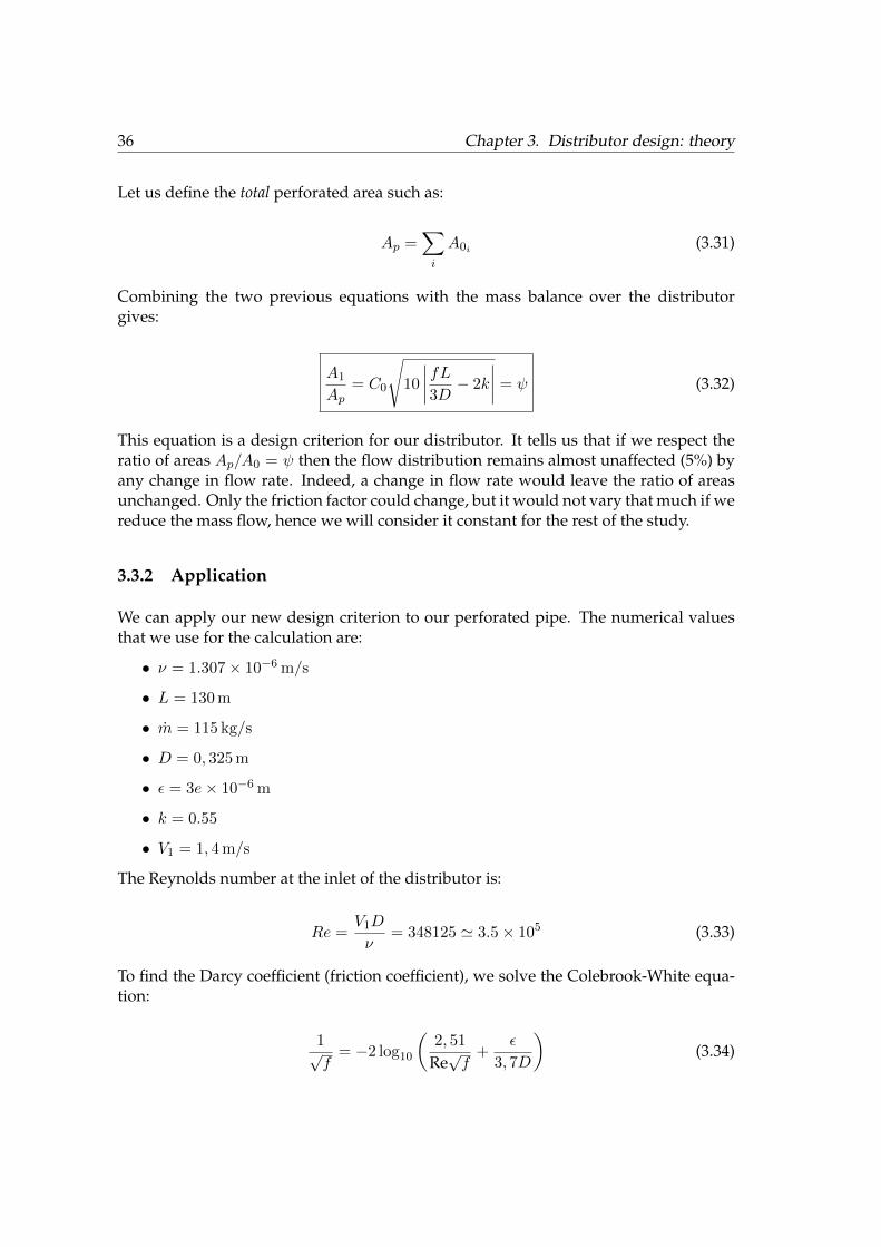
Let us define the total perforated area such as:
Ap =∑i
A0i (3.31)
Combining the two previous equations with the mass balance over the distributorgives:
A1
Ap= C0
√10
∣∣∣∣ fL3D− 2k
∣∣∣∣ = ψ (3.32)
This equation is a design criterion for our distributor. It tells us that if we respect theratio of areas Ap/A0 = ψ then the flow distribution remains almost unaffected (5%) byany change in flow rate. Indeed, a change in flow rate would leave the ratio of areasunchanged. Only the friction factor could change, but it would not vary that much if wereduce the mass flow, hence we will consider it constant for the rest of the study.
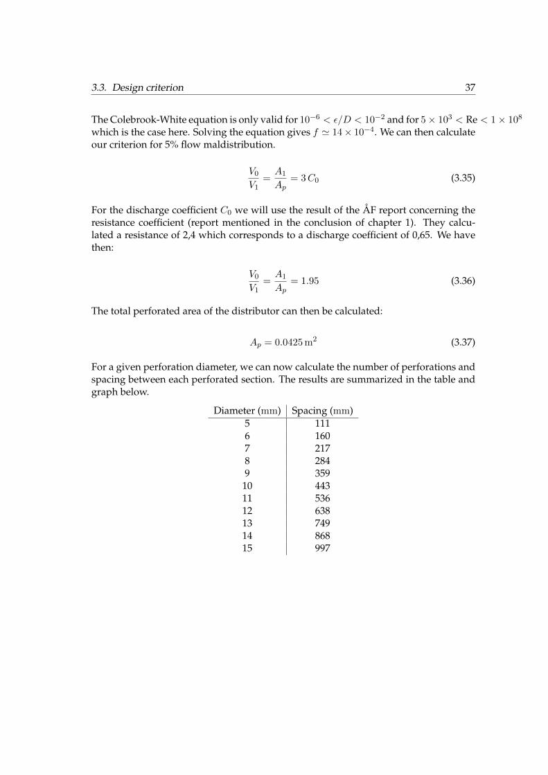
3.3.2 Application
We can apply our new design criterion to our perforated pipe. The numerical valuesthat we use for the calculation are:
• ν = 1.307× 10⁻⁶ m/s
• L = 130 m
• m = 115 kg/s
• D = 0, 325 m
• ε = 3e× 10−6 m
• k = 0.55
• V1 = 1, 4 m/s
The Reynolds number at the inlet of the distributor is:
Re =V1D
ν= 348125 ' 3.5× 10⁵ (3.33)
To find the Darcy coefficient (friction coefficient), we solve the Colebrook-White equa-tion:
1√f
= −2 log10
(2, 51
Re√f
+ε
3, 7D
)(3.34)
3.3. Design criterion 37
The Colebrook-White equation is only valid for 10−6 < ε/D < 10−2 and for 5× 10³ < Re < 1× 10⁸
which is the case here. Solving the equation gives f ' 14× 10−4. We can then calculateour criterion for 5% flow maldistribution.
V0V1
=A1
Ap= 3C0 (3.35)
For the discharge coefficient C0 we will use the result of the ÅF report concerning theresistance coefficient (report mentioned in the conclusion of chapter 1). They calcu-lated a resistance of 2,4 which corresponds to a discharge coefficient of 0,65. We havethen:
V0V1
=A1
Ap= 1.95 (3.36)
The total perforated area of the distributor can then be calculated:
Ap = 0.0425 m2 (3.37)
For a given perforation diameter, we can now calculate the number of perforations andspacing between each perforated section. The results are summarized in the table andgraph below.
Diameter (mm) Spacing (mm)5 1116 1607 2178 2849 359
10 44311 53612 63813 74914 86815 997
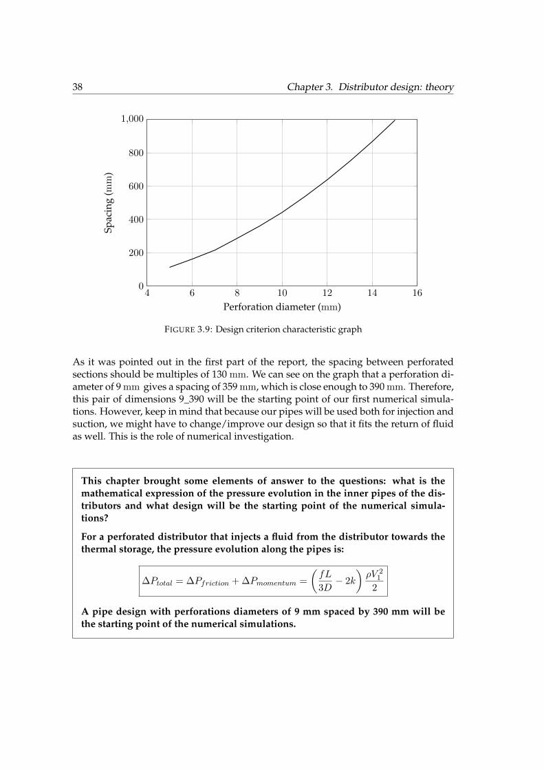
38 Chapter 3. Distributor design: theory
4 6 8 10 12 14 160
200
400
600
800
1,000
Perforation diameter (mm)
Spac
ing
(mm
)
FIGURE 3.9: Design criterion characteristic graph
As it was pointed out in the first part of the report, the spacing between perforatedsections should be multiples of 130 mm. We can see on the graph that a perforation di-ameter of 9 mm gives a spacing of 359 mm, which is close enough to 390 mm. Therefore,this pair of dimensions 9_390 will be the starting point of our first numerical simula-tions. However, keep in mind that because our pipes will be used both for injection andsuction, we might have to change/improve our design so that it fits the return of fluidas well. This is the role of numerical investigation.
This chapter brought some elements of answer to the questions: what is themathematical expression of the pressure evolution in the inner pipes of the dis-tributors and what design will be the starting point of the numerical simula-tions?
For a perforated distributor that injects a fluid from the distributor towards thethermal storage, the pressure evolution along the pipes is:
∆Ptotal = ∆Pfriction + ∆Pmomentum =
(fL
3D− 2k
)ρV 2
1
2
A pipe design with perforations diameters of 9 mm spaced by 390 mm will bethe starting point of the numerical simulations.
39
Chapter 4
Distributor design: simulations
This chapter consists of two sections. The first section concerns the study ofthe inner pipe. The second section details the results of the conducted sen-sitivity analysis. We will answer the following questions: are the numericalresults correlating the theory, and what design is recommended for the waterdistributors?
4.1 Verification of the theory
4.1.1 Geometry and meshing
Because numerical simulations are time consuming, it is important to make soundschoices when it comes to the geometry we want to consider, mesh and use. Instead ofmodeling the entire distributor (inner and outer tubes) we will in the first place studyonly the flow of water throughout the inner tube only and running out of the smallperforations. However is it important for that part to consider the inner tube over itsentire length, since we are interested in the pressure evolution over the entire tube. Thatfirst part will give us information about the flow distribution in and out of the innertube, which is directly connected to the flow distribution in the water storage.
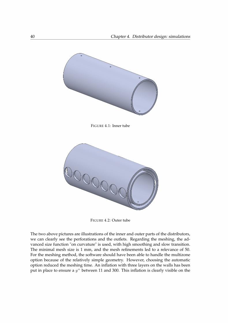
40 Chapter 4. Distributor design: simulations
FIGURE 4.1: Inner tube
FIGURE 4.2: Outer tube
The two above pictures are illustrations of the inner and outer parts of the distributors,we can clearly see the perforations and the outlets. Regarding the meshing, the ad-vanced size function "on curvature" is used, with high smoothing and slow transition.The minimal mesh size is 1 mm, and the mesh refinements led to a relevance of 50.For the meshing method, the software should have been able to handle the multizoneoption because of the relatively simple geometry. However, choosing the automaticoption reduced the meshing time. An inflation with three layers on the walls has beenput in place to ensure a y+ between 11 and 300. This inflation is clearly visible on the
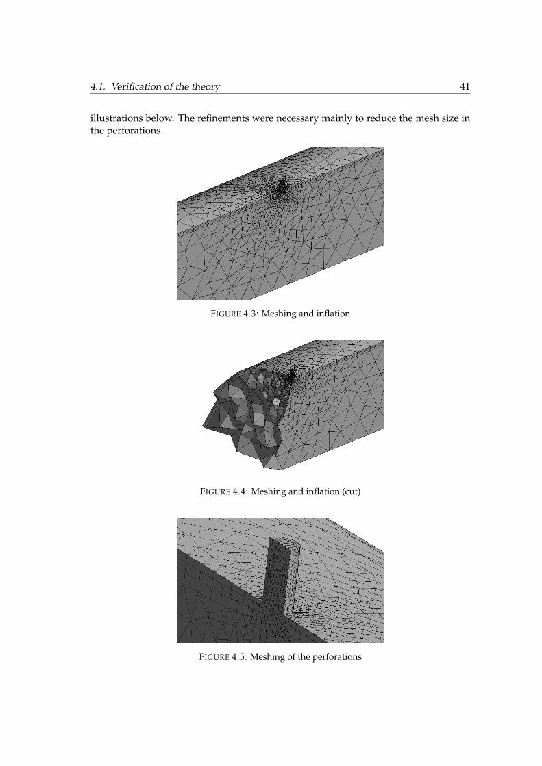
4.1. Verification of the theory 41
illustrations below. The refinements were necessary mainly to reduce the mesh size inthe perforations.
FIGURE 4.3: Meshing and inflation
FIGURE 4.4: Meshing and inflation (cut)
FIGURE 4.5: Meshing of the perforations
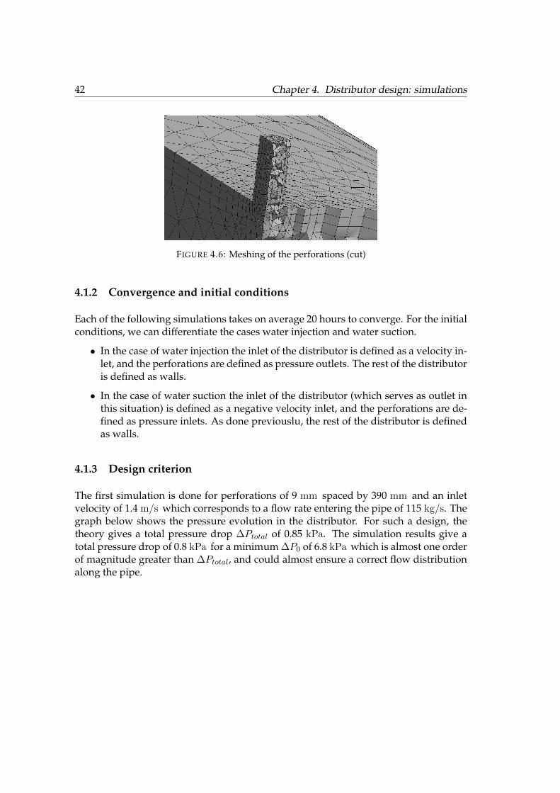
42 Chapter 4. Distributor design: simulations
FIGURE 4.6: Meshing of the perforations (cut)
4.1.2 Convergence and initial conditions
Each of the following simulations takes on average 20 hours to converge. For the initialconditions, we can differentiate the cases water injection and water suction.
• In the case of water injection the inlet of the distributor is defined as a velocity in-let, and the perforations are defined as pressure outlets. The rest of the distributoris defined as walls.
• In the case of water suction the inlet of the distributor (which serves as outlet inthis situation) is defined as a negative velocity inlet, and the perforations are de-fined as pressure inlets. As done previouslu, the rest of the distributor is definedas walls.
4.1.3 Design criterion
The first simulation is done for perforations of 9 mm spaced by 390 mm and an inletvelocity of 1.4 m/s which corresponds to a flow rate entering the pipe of 115 kg/s. Thegraph below shows the pressure evolution in the distributor. For such a design, thetheory gives a total pressure drop ∆Ptotal of 0.85 kPa. The simulation results give atotal pressure drop of 0.8 kPa for a minimum ∆P0 of 6.8 kPa which is almost one orderof magnitude greater than ∆Ptotal, and could almost ensure a correct flow distributionalong the pipe.
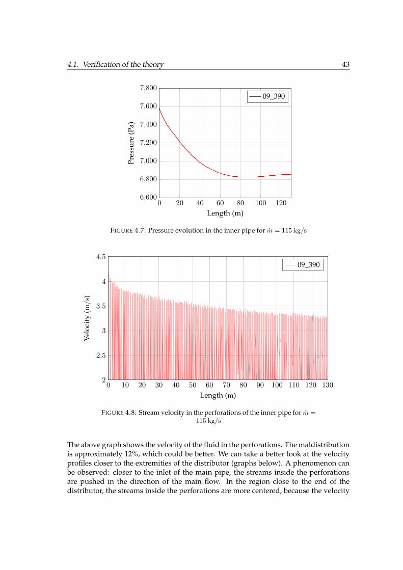
4.1. Verification of the theory 43
0 20 40 60 80 100 1206,600
6,800
7,000
7,200
7,400
7,600
7,800
Length (m)
Pres
sure
(Pa)
09_390
FIGURE 4.7: Pressure evolution in the inner pipe for m = 115 kg/s
0 10 20 30 40 50 60 70 80 90 100 110 120 1302
2.5
3
3.5
4
4.5
Length (m)
Velo
city
(m/s)
09_390
FIGURE 4.8: Stream velocity in the perforations of the inner pipe for m =115 kg/s
The above graph shows the velocity of the fluid in the perforations. The maldistributionis approximately 12%, which could be better. We can take a better look at the velocityprofiles closer to the extremities of the distributor (graphs below). A phenomenon canbe observed: closer to the inlet of the main pipe, the streams inside the perforationsare pushed in the direction of the main flow. In the region close to the end of thedistributor, the streams inside the perforations are more centered, because the velocity
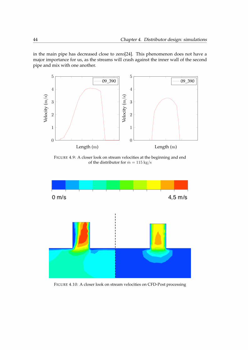
44 Chapter 4. Distributor design: simulations
in the main pipe has decreased close to zero[24]. This phenomenon does not have amajor importance for us, as the streams will crash against the inner wall of the secondpipe and mix with one another.
0
1
2
3
4
5
Length (m)
Velo
city
(m/s)
09_390
0
1
2
3
4
5
Length (m)
Velo
city
(m/s
)
09_390
FIGURE 4.9: A closer look on stream velocities at the beginning and endof the distributor for m = 115 kg/s
FIGURE 4.10: A closer look on stream velocities on CFD-Post processing
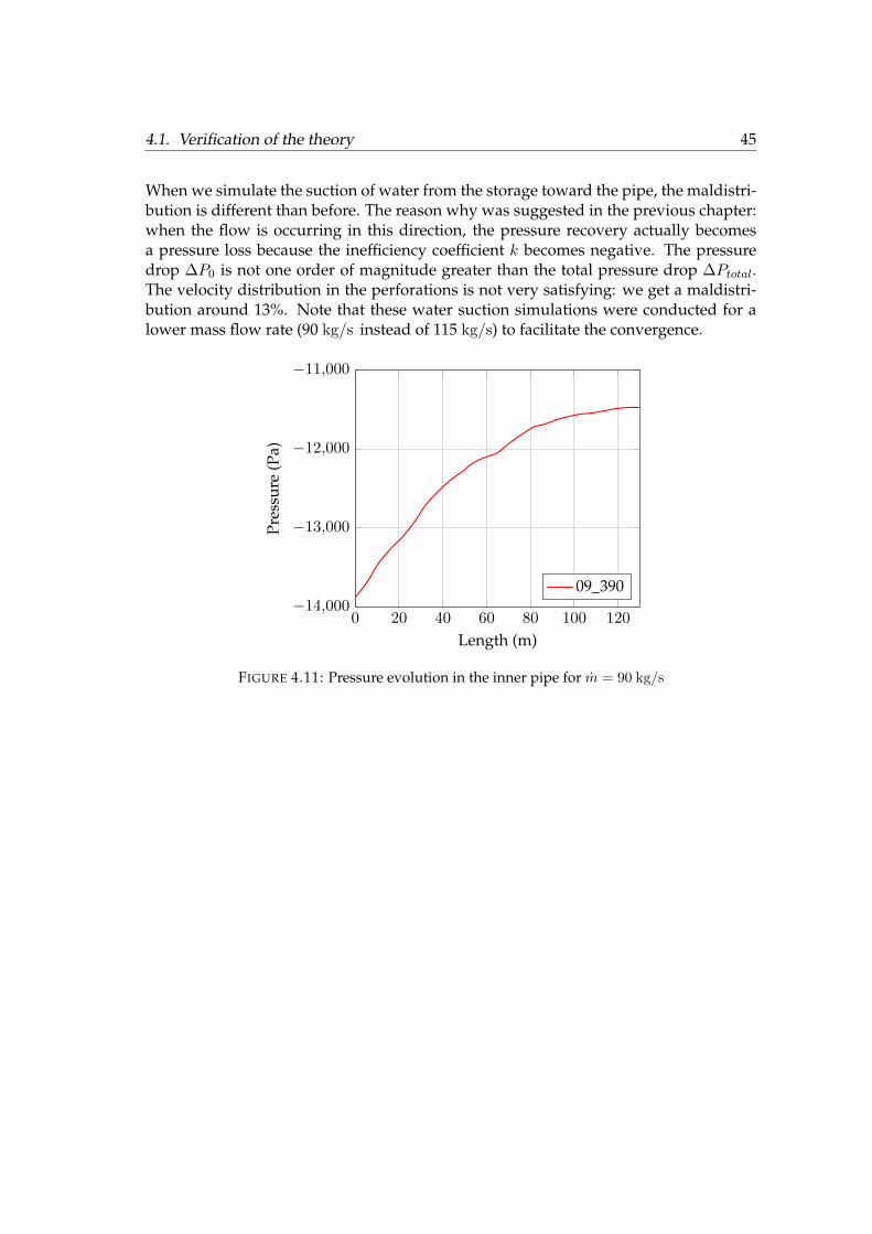
4.1. Verification of the theory 45
When we simulate the suction of water from the storage toward the pipe, the maldistri-bution is different than before. The reason why was suggested in the previous chapter:when the flow is occurring in this direction, the pressure recovery actually becomesa pressure loss because the inefficiency coefficient k becomes negative. The pressuredrop ∆P0 is not one order of magnitude greater than the total pressure drop ∆Ptotal.The velocity distribution in the perforations is not very satisfying: we get a maldistri-bution around 13%. Note that these water suction simulations were conducted for alower mass flow rate (90 kg/s instead of 115 kg/s) to facilitate the convergence.
0 20 40 60 80 100 120−14,000
−13,000
−12,000
−11,000
Length (m)
Pres
sure
(Pa)
09_390
FIGURE 4.11: Pressure evolution in the inner pipe for m = 90 kg/s
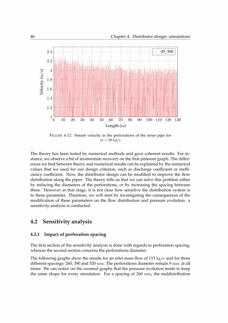
46 Chapter 4. Distributor design: simulations
0 10 20 30 40 50 60 70 80 90 100 110 120 1301
1.2
1.4
1.6
1.8
2
2.2
2.4
Length (m)
Velo
city
(m/s
)
09_390
FIGURE 4.12: Stream velocity in the perforations of the inner pipe form = 90 kg/s
The theory has been tested by numerical methods and gave coherent results. For in-stance, we observe a bit of momentum recovery on the first pressure graph. The differ-ences we find between theory and numerical results can be explained by the numericalvalues that we used for our design criterion, such as discharge coefficient or ineffi-ciency coefficient. Now, the distributor design can be modified to improve the flowdistribution along the pipes. The theory tells us that we can solve this problem eitherby reducing the diameters of the perforations, or by increasing the spacing betweenthem. However at that stage, it is not clear how sensitive the distribution system isto these parameter. Therefore, we will start by investigating the consequences of themodification of these parameters on the flow distribution and pressure evolution: asensitivity analysis is conducted.
4.2 Sensitivity analysis
4.2.1 Impact of perforation spacing
The first section of the sensitivity analysis is done with regards to perforation spacing,whereas the second section concerns the perforations diameter.
The following graphs show the results for an inlet mass flow of 115 kg/s and for threedifferent spacings: 260, 390 and 520 mm. The perforations diameter remain 9 mm at alltimes. We can notice on the zoomed graphs that the pressure evolution tends to keepthe same shape for every simulation. For a spacing of 260 mm, the maldistribution
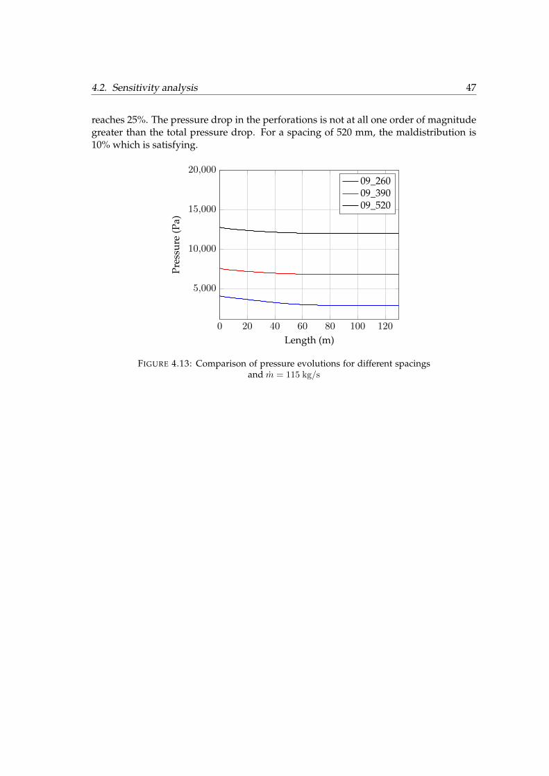
4.2. Sensitivity analysis 47
reaches 25%. The pressure drop in the perforations is not at all one order of magnitudegreater than the total pressure drop. For a spacing of 520 mm, the maldistribution is10% which is satisfying.
0 20 40 60 80 100 120
5,000
10,000
15,000
20,000
Length (m)
Pres
sure
(Pa)
09_26009_39009_520
FIGURE 4.13: Comparison of pressure evolutions for different spacingsand m = 115 kg/s
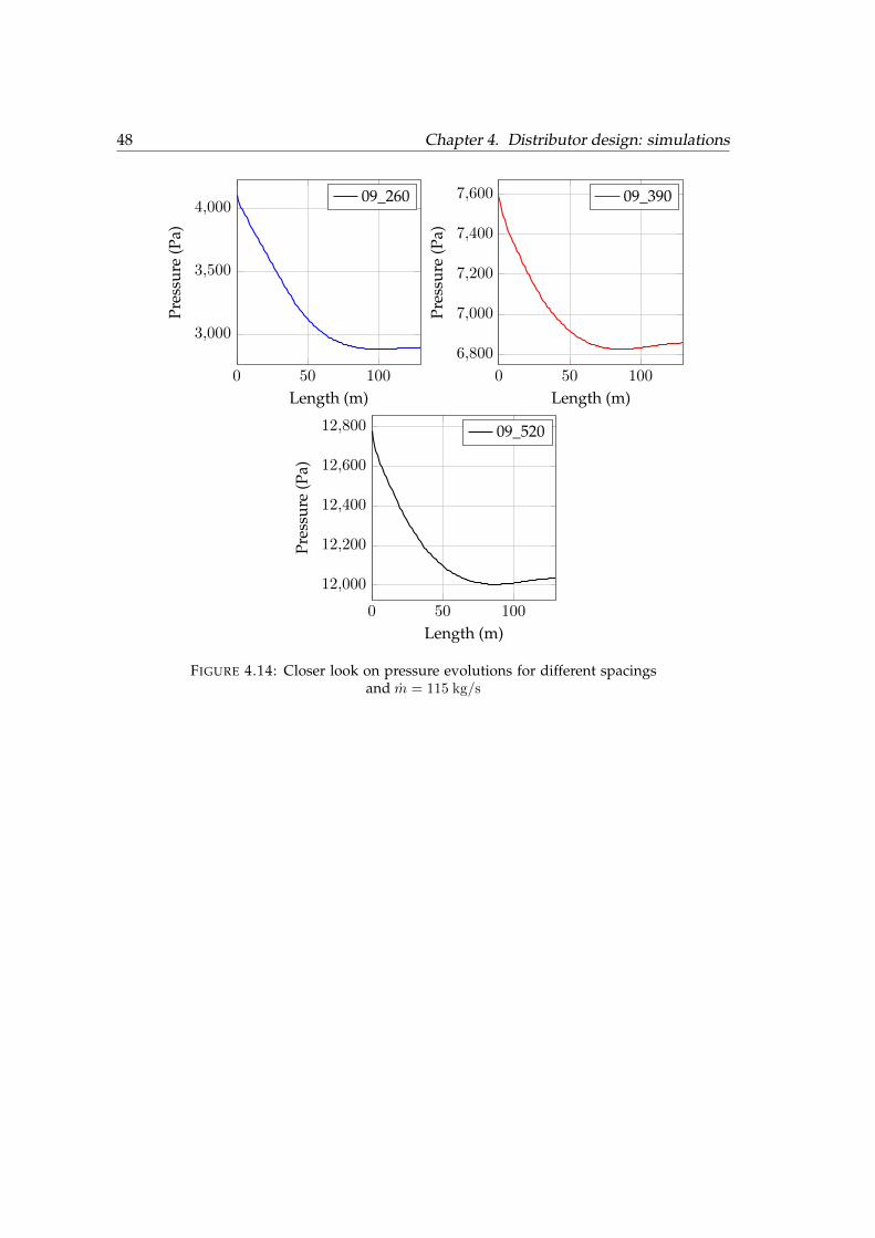
48 Chapter 4. Distributor design: simulations
0 50 100
3,000
3,500
4,000
Length (m)
Pres
sure
(Pa)
09_260
0 50 100
6,800
7,000
7,200
7,400
7,600
Length (m)
Pres
sure
(Pa)
09_390
0 50 100
12,000
12,200
12,400
12,600
12,800
Length (m)
Pres
sure
(Pa)
09_520
FIGURE 4.14: Closer look on pressure evolutions for different spacingsand m = 115 kg/s
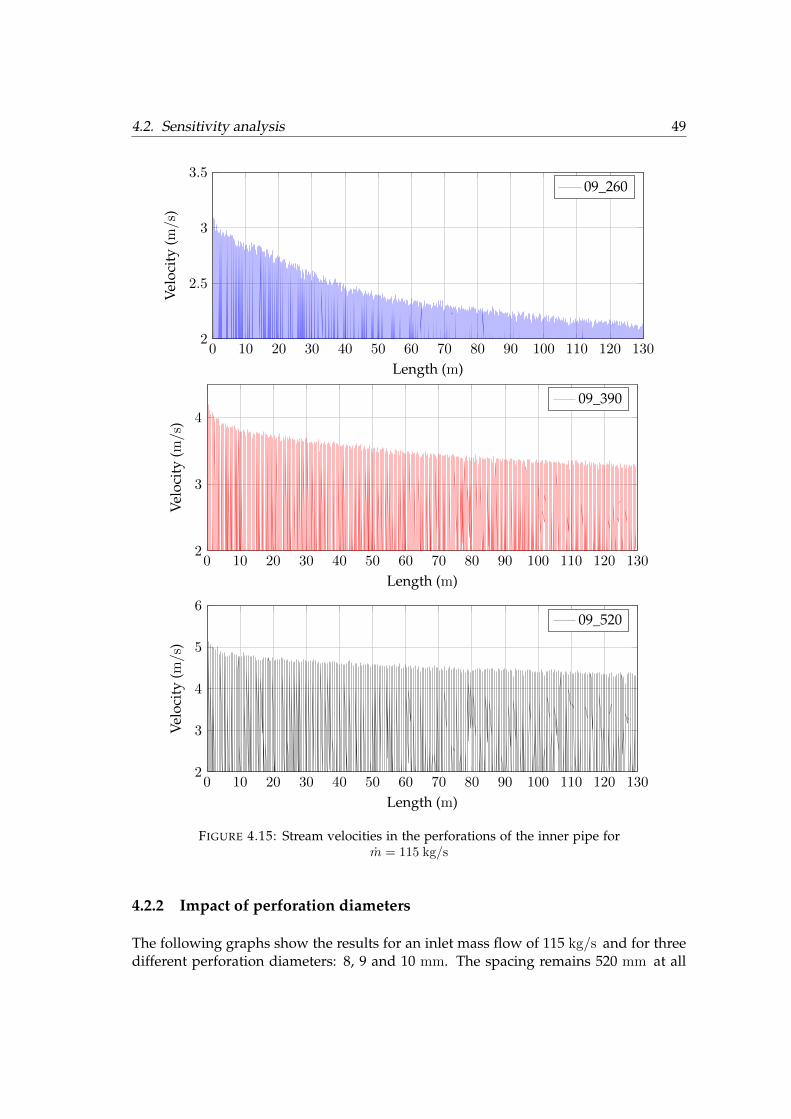
4.2. Sensitivity analysis 49
0 10 20 30 40 50 60 70 80 90 100 110 120 1302
2.5
3
3.5
Length (m)
Velo
city
(m/s)
09_260
0 10 20 30 40 50 60 70 80 90 100 110 120 1302
3
4
Length (m)
Velo
city
(m/s
)
09_390
0 10 20 30 40 50 60 70 80 90 100 110 120 1302
3
4
5
6
Length (m)
Velo
city
(m/s
)
09_520
FIGURE 4.15: Stream velocities in the perforations of the inner pipe form = 115 kg/s
4.2.2 Impact of perforation diameters
The following graphs show the results for an inlet mass flow of 115 kg/s and for threedifferent perforation diameters: 8, 9 and 10 mm. The spacing remains 520 mm at all
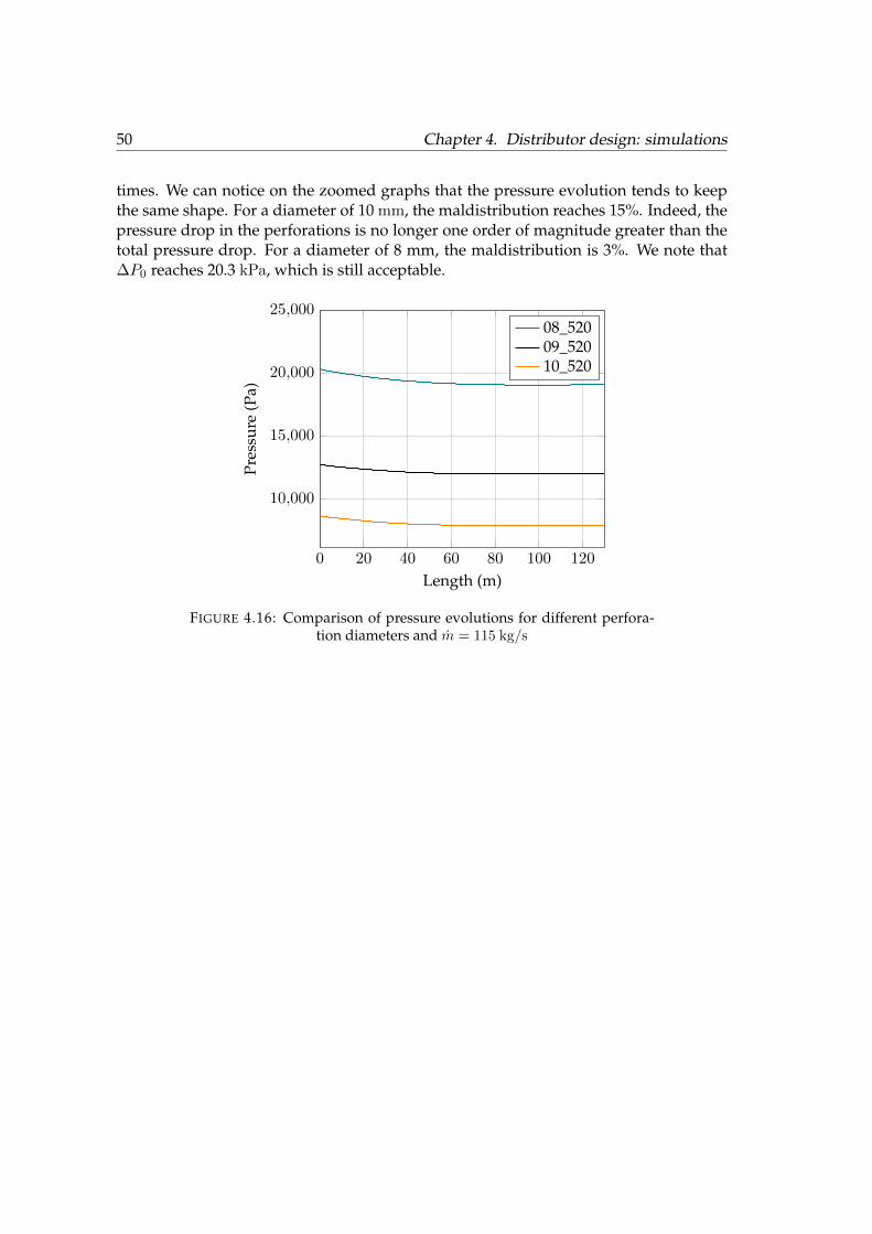
50 Chapter 4. Distributor design: simulations
times. We can notice on the zoomed graphs that the pressure evolution tends to keepthe same shape. For a diameter of 10 mm, the maldistribution reaches 15%. Indeed, thepressure drop in the perforations is no longer one order of magnitude greater than thetotal pressure drop. For a diameter of 8 mm, the maldistribution is 3%. We note that∆P0 reaches 20.3 kPa, which is still acceptable.
0 20 40 60 80 100 120
10,000
15,000
20,000
25,000
Length (m)
Pres
sure
(Pa)
08_52009_52010_520
FIGURE 4.16: Comparison of pressure evolutions for different perfora-tion diameters and m = 115 kg/s
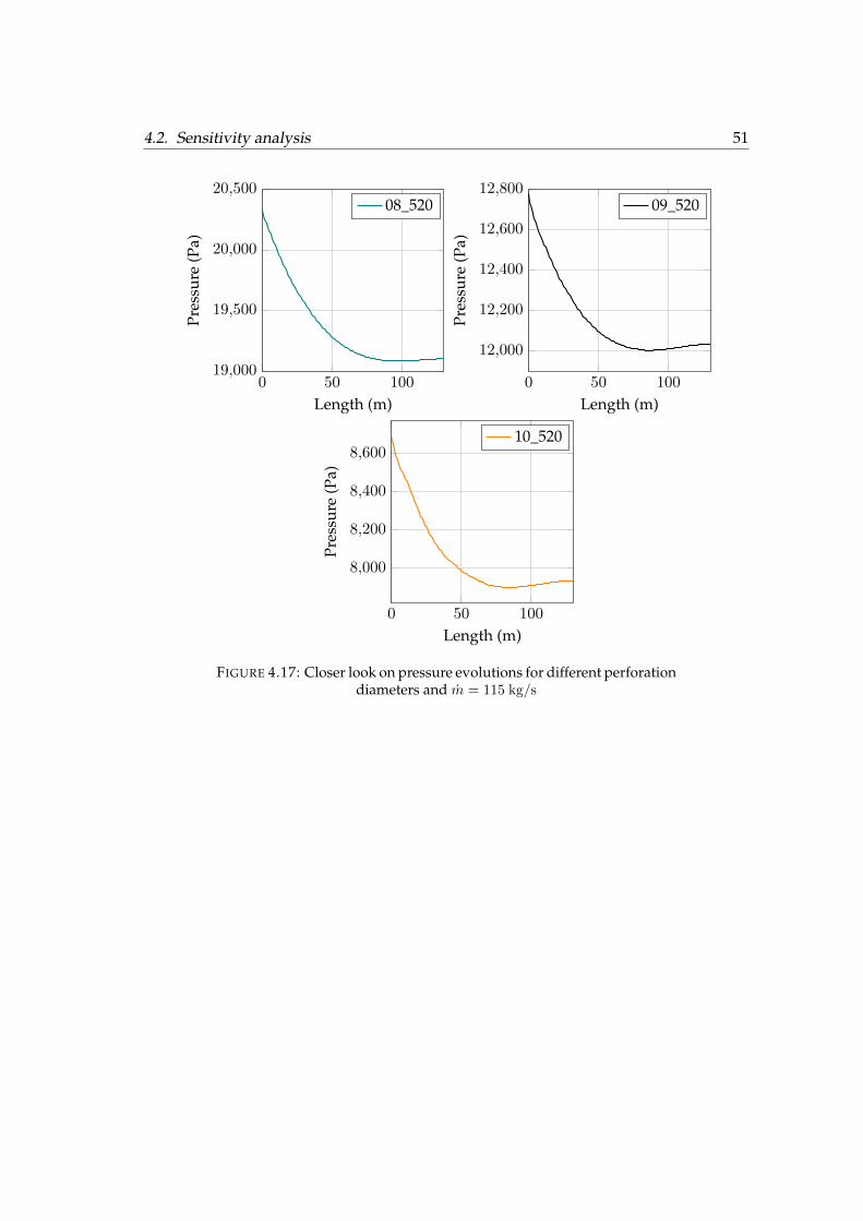
4.2. Sensitivity analysis 51
0 50 10019,000
19,500
20,000
20,500
Length (m)
Pres
sure
(Pa)
08_520
0 50 100
12,000
12,200
12,400
12,600
12,800
Length (m)
Pres
sure
(Pa)
09_520
0 50 100
8,000
8,200
8,400
8,600
Length (m)
Pres
sure
(Pa)
10_520
FIGURE 4.17: Closer look on pressure evolutions for different perforationdiameters and m = 115 kg/s

52 Chapter 4. Distributor design: simulations
0 10 20 30 40 50 60 70 80 90 100 110 120 1302
4
6
Length (m)
Velo
city
(m/s)
08_520
0 10 20 30 40 50 60 70 80 90 100 110 120 1302
3
4
5
6
Length (m)
Velo
city
(m/s)
09_520
0 10 20 30 40 50 60 70 80 90 100 110 120 1302
3
4
5
Length (m)
Velo
city
(m/s)
10_520
FIGURE 4.18: Stream velocities in the perforations of the inner pipe form = 115 kg/s
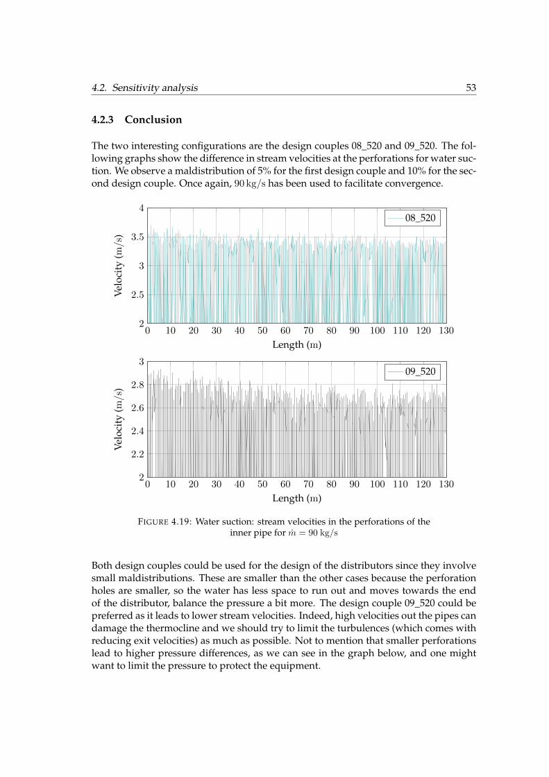
4.2. Sensitivity analysis 53
4.2.3 Conclusion
The two interesting configurations are the design couples 08_520 and 09_520. The fol-lowing graphs show the difference in stream velocities at the perforations for water suc-tion. We observe a maldistribution of 5% for the first design couple and 10% for the sec-ond design couple. Once again, 90 kg/s has been used to facilitate convergence.
0 10 20 30 40 50 60 70 80 90 100 110 120 1302
2.5
3
3.5
4
Length (m)
Velo
city
(m/s)
08_520
0 10 20 30 40 50 60 70 80 90 100 110 120 1302
2.2
2.4
2.6
2.8
3
Length (m)
Velo
city
(m/s)
09_520
FIGURE 4.19: Water suction: stream velocities in the perforations of theinner pipe for m = 90 kg/s
Both design couples could be used for the design of the distributors since they involvesmall maldistributions. These are smaller than the other cases because the perforationholes are smaller, so the water has less space to run out and moves towards the endof the distributor, balance the pressure a bit more. The design couple 09_520 could bepreferred as it leads to lower stream velocities. Indeed, high velocities out the pipes candamage the thermocline and we should try to limit the turbulences (which comes withreducing exit velocities) as much as possible. Not to mention that smaller perforationslead to higher pressure differences, as we can see in the graph below, and one mightwant to limit the pressure to protect the equipment.
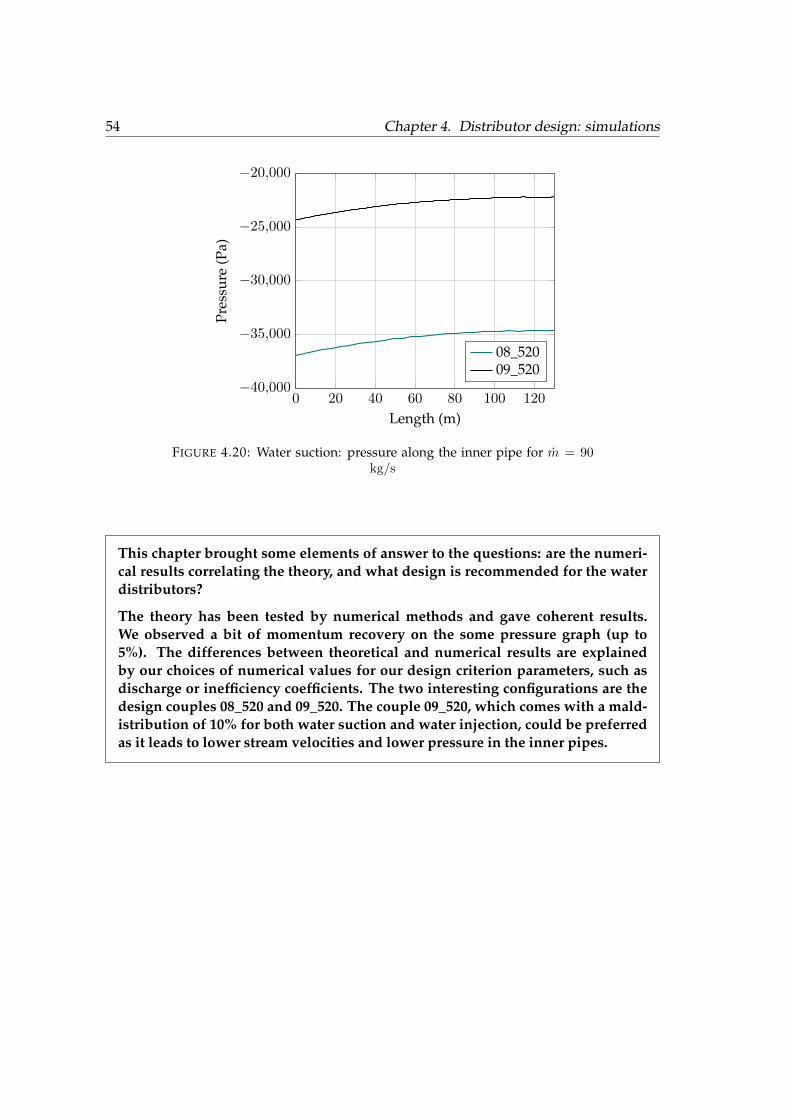
54 Chapter 4. Distributor design: simulations
0 20 40 60 80 100 120−40,000
−35,000
−30,000
−25,000
−20,000
Length (m)
Pres
sure
(Pa)
08_52009_520
FIGURE 4.20: Water suction: pressure along the inner pipe for m = 90kg/s
This chapter brought some elements of answer to the questions: are the numeri-cal results correlating the theory, and what design is recommended for the waterdistributors?
The theory has been tested by numerical methods and gave coherent results.We observed a bit of momentum recovery on the some pressure graph (up to5%). The differences between theoretical and numerical results are explainedby our choices of numerical values for our design criterion parameters, such asdischarge or inefficiency coefficients. The two interesting configurations are thedesign couples 08_520 and 09_520. The couple 09_520, which comes with a mald-istribution of 10% for both water suction and water injection, could be preferredas it leads to lower stream velocities and lower pressure in the inner pipes.
55
Chapter 5
Thermocline evolution
This chapter consists of three sections. The first section is an introduction to ther-mocline formation and conservation. The second and third sections present theresults of the numerical investigations. We will answer the following questions:what is the influence of the number of pipes and of the flow rates characteristicson thermocline formation and evolution?
5.1 Different challenges
5.1.1 Dependency on distributor design
In the previous chapter, we conducted a numerical investigation regarding the perfo-rated distributors that led to the following design:
• Perforations diameter of 9 mm;
• Spacing of 540 mm between each perforations.
Originally, ÅF suggested 3 distributors on the top and 3 on the bottom of the cave.Having many pipes facilitates the formation of the thermocline (which we discuss lateron in this chapter) and presents the advantage of reducing the velocities at the outlets(for a same main mass flow rate flowing in and out of the storage of course). But addingpipes also makes the project more expensive, therefore it is necessary to investigate thequestion of the required pipes number. In order to do so, we will answer the followinginterrogations:
• What is the influence of the number of pipes on thermocline formation?
• What is the influence of the number of pipes on thermocline evolution and preser-vation during charging/discharging cycles?
To begin with, it is important to understand that the maximal mass flow rate (in and outof the storage) is determined by the distance that the thermocline can travel during afull charging/discharging cycle. The thermocline should remain at a fair distance away
56 Chapter 5. Thermocline evolution
from the pipes during the cycles. Indeed the turbulences close to the distributors mightdamage severely the temperature gradient layer. Let us consider a maximum mass flowrate in and out of the storage of m = 450 kg/s. This is a reasonable assumption for thisstorage. The details on load profiles, average and maximal mass flow rates are given inthe section Thermocline formation (5.2).
The average velocity out of one outlet depends on m and on the total outlets area. Eachdistributor of 130 m long presents 2000 outlets. For 3 distributors, this means 6000outlets. Finally we can calculate the average velocity at one outlet:
v =m
ρ× 6000× π×φ24
(5.1)
v =450
999, 8× 6000× π×0.112
4
' 8 mm/s (5.2)
However, because of its profile at the outlets, the average velocity v can easily be mul-tiplied by 3 in order to get the maximal velocity. This is the velocity we are interestedin here, because it is the one that will create the largest eddies and that will determinethe flow regime (see chapter 2 on turbulences for more details). Hence we will use 3v,which leads to a Reynolds number of:
Re3 =ρ 3v φ
ν' 2640 (5.3)
That number is somewhere between the transition and turbulent regions. It is verydifficult to predict exactly the nature of the flow, however this is still a very helpfulinformation for decision making. If we consider now 5 distributors instead of 3, theprevious calculation simply becomes:
Re5 =ρ 3v φ
ν× 3
5' 1580 (5.4)
Which is somewhere between the laminar and transition region (once again, difficultto tell as we can’t predict exactly the behavior of the flow between the inner and outerpipes). This first approach tells us that 5 pipes might make a significant difference inthe level of turbulences at the outlets, but is it really the case? Simulations need to berun to push further the investigation.
5.1.2 Formation and conservation
Consider the thermal storage entirely filled with cold water at 4◦C. The process of fill-ing the top of the tank with warm water at 14◦C is called thermocline formation, andshould not be neglected. In fact, the initial thermocline thickness depends directly on
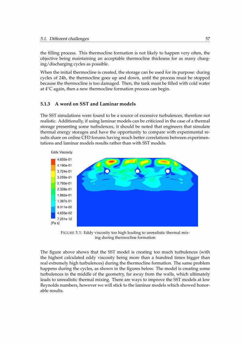
5.1. Different challenges 57
the filling process. This thermocline formation is not likely to happen very often, theobjective being maintaining an acceptable thermocline thickness for as many charg-ing/discharging cycles as possible.
When the initial thermocline is created, the storage can be used for its purpose: duringcycles of 24h, the thermocline goes up and down, until the process must be stoppedbecause the thermocline is too damaged. Then, the tank must be filled with cold waterat 4◦C again, then a new thermocline formation process can begin.
5.1.3 A word on SST and Laminar models
The SST simulations were found to be a source of excessive turbulences, therefore notrealistic. Additionally, if using laminar models can be criticized in the case of a thermalstorage presenting some turbulences, it should be noted that engineers that simulatethermal energy storages and have the opportunity to compare with experimental re-sults share on online CFD forums having much better correlations between experimen-tations and laminar models results rather than with SST models.
FIGURE 5.1: Eddy viscosity too high leading to unrealistic thermal mix-ing during thermocline formation
The figure above shows that the SST model is creating too much turbulences (withthe highest calculated eddy viscosity being more than a hundred times bigger thanreal extremely high turbulences) during the thermocline formation. The same problemhappens during the cycles, as shown in the figures below. The model is creating someturbulences in the middle of the geometry, far away from the walls, which ultimatelyleads to unrealistic thermal mixing. There are ways to improve the SST models at lowReynolds numbers, however we will stick to the laminar models which showed honor-able results.
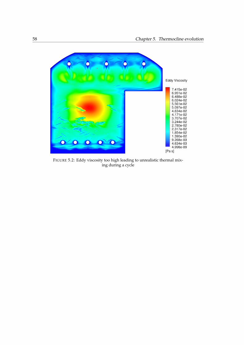
58 Chapter 5. Thermocline evolution
FIGURE 5.2: Eddy viscosity too high leading to unrealistic thermal mix-ing during a cycle
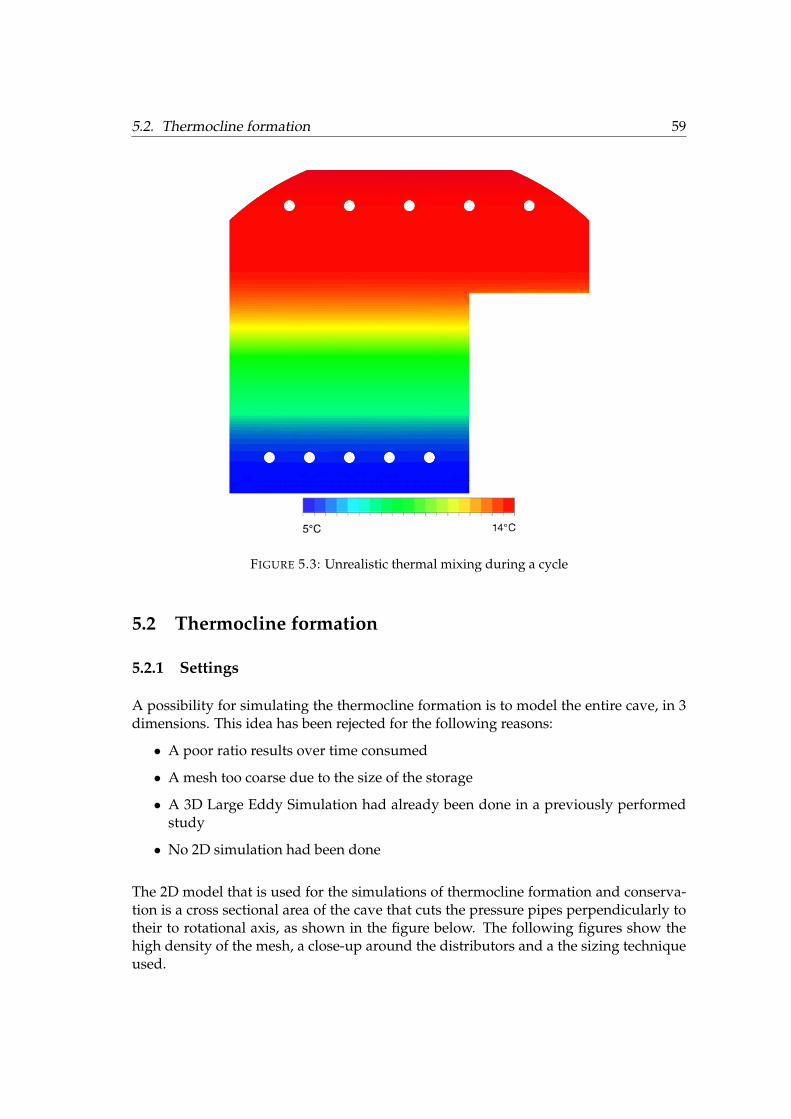
5.2. Thermocline formation 59
FIGURE 5.3: Unrealistic thermal mixing during a cycle
5.2 Thermocline formation
5.2.1 Settings
A possibility for simulating the thermocline formation is to model the entire cave, in 3dimensions. This idea has been rejected for the following reasons:
• A poor ratio results over time consumed
• A mesh too coarse due to the size of the storage
• A 3D Large Eddy Simulation had already been done in a previously performedstudy
• No 2D simulation had been done
The 2D model that is used for the simulations of thermocline formation and conserva-tion is a cross sectional area of the cave that cuts the pressure pipes perpendicularly totheir to rotational axis, as shown in the figure below. The following figures show thehigh density of the mesh, a close-up around the distributors and a the sizing techniqueused.
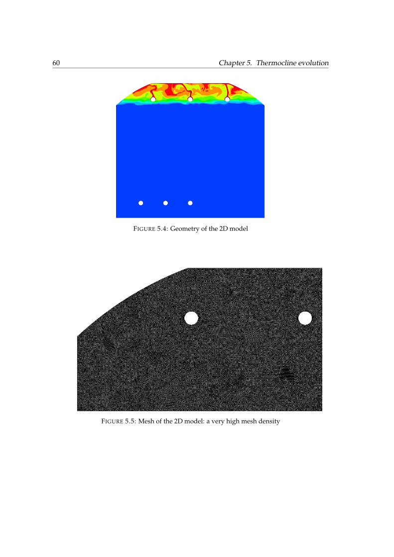
60 Chapter 5. Thermocline evolution
FIGURE 5.4: Geometry of the 2D model
FIGURE 5.5: Mesh of the 2D model: a very high mesh density
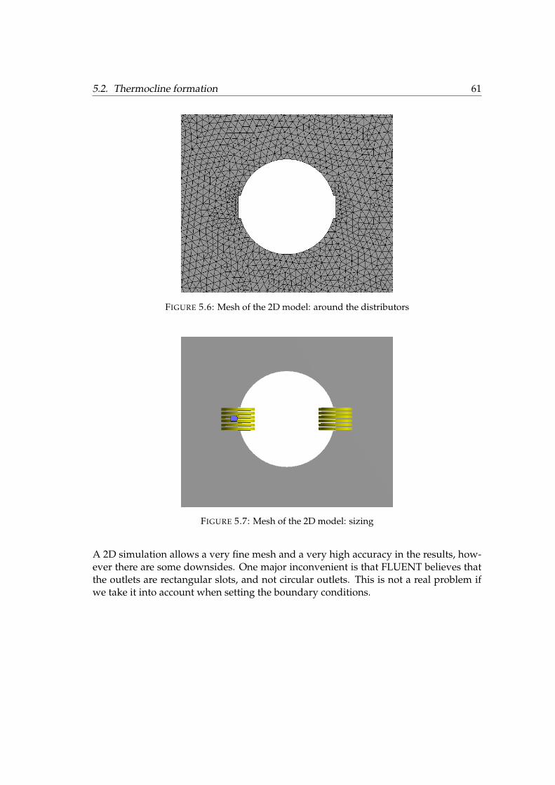
5.2. Thermocline formation 61
FIGURE 5.6: Mesh of the 2D model: around the distributors
FIGURE 5.7: Mesh of the 2D model: sizing
A 2D simulation allows a very fine mesh and a very high accuracy in the results, how-ever there are some downsides. One major inconvenient is that FLUENT believes thatthe outlets are rectangular slots, and not circular outlets. This is not a real problem ifwe take it into account when setting the boundary conditions.
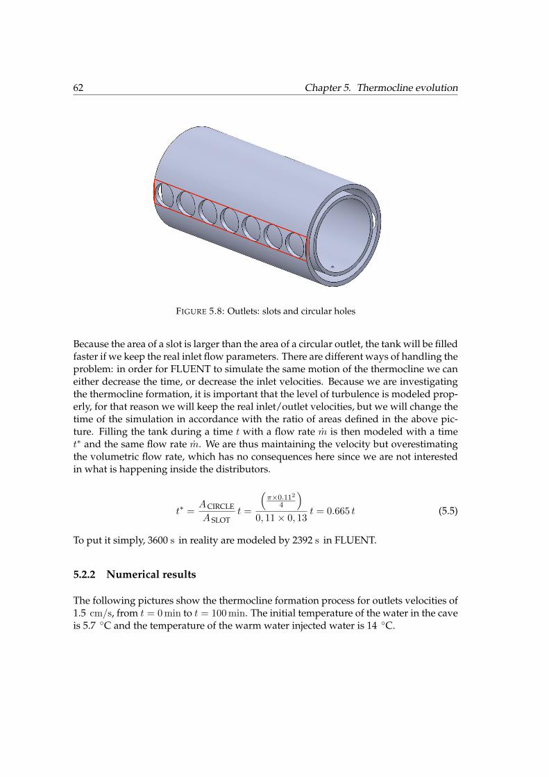
62 Chapter 5. Thermocline evolution
FIGURE 5.8: Outlets: slots and circular holes
Because the area of a slot is larger than the area of a circular outlet, the tank will be filledfaster if we keep the real inlet flow parameters. There are different ways of handling theproblem: in order for FLUENT to simulate the same motion of the thermocline we caneither decrease the time, or decrease the inlet velocities. Because we are investigatingthe thermocline formation, it is important that the level of turbulence is modeled prop-erly, for that reason we will keep the real inlet/outlet velocities, but we will change thetime of the simulation in accordance with the ratio of areas defined in the above pic-ture. Filling the tank during a time t with a flow rate m is then modeled with a timet∗ and the same flow rate m. We are thus maintaining the velocity but overestimatingthe volumetric flow rate, which has no consequences here since we are not interestedin what is happening inside the distributors.
t∗ =ACIRCLE
A SLOTt =
(π×0.112
4
)0, 11× 0, 13
t = 0.665 t (5.5)
To put it simply, 3600 s in reality are modeled by 2392 s in FLUENT.
5.2.2 Numerical results
The following pictures show the thermocline formation process for outlets velocities of1.5 cm/s, from t = 0 min to t = 100 min. The initial temperature of the water in the caveis 5.7 ◦C and the temperature of the warm water injected water is 14 ◦C.
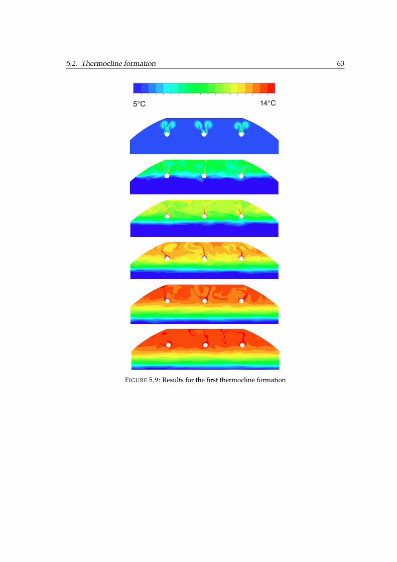
5.2. Thermocline formation 63
FIGURE 5.9: Results for the first thermocline formation
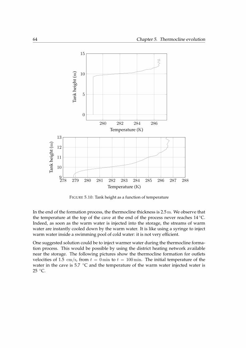
64 Chapter 5. Thermocline evolution
280 282 284 286
0
5
10
15
Temperature (K)
Tank
heig
ht(m
)
278 279 280 281 282 283 284 285 286 287 2889
10
11
12
13
Temperature (K)
Tank
heig
ht(m
)
FIGURE 5.10: Tank height as a function of temperature
In the end of the formation process, the thermocline thickness is 2.5 m. We observe thatthe temperature at the top of the cave at the end of the process never reaches 14 ◦C.Indeed, as soon as the warm water is injected into the storage, the streams of warmwater are instantly cooled down by the warm water. It is like using a syringe to injectwarm water inside a swimming pool of cold water: it is not very efficient.
One suggested solution could be to inject warmer water during the thermocline forma-tion process. This would be possible by using the district heating network availablenear the storage. The following pictures show the thermocline formation for outletsvelocities of 1.5 cm/s, from t = 0 min to t = 100 min. The initial temperature of thewater in the cave is 5.7 ◦C and the temperature of the warm water injected water is25 ◦C.
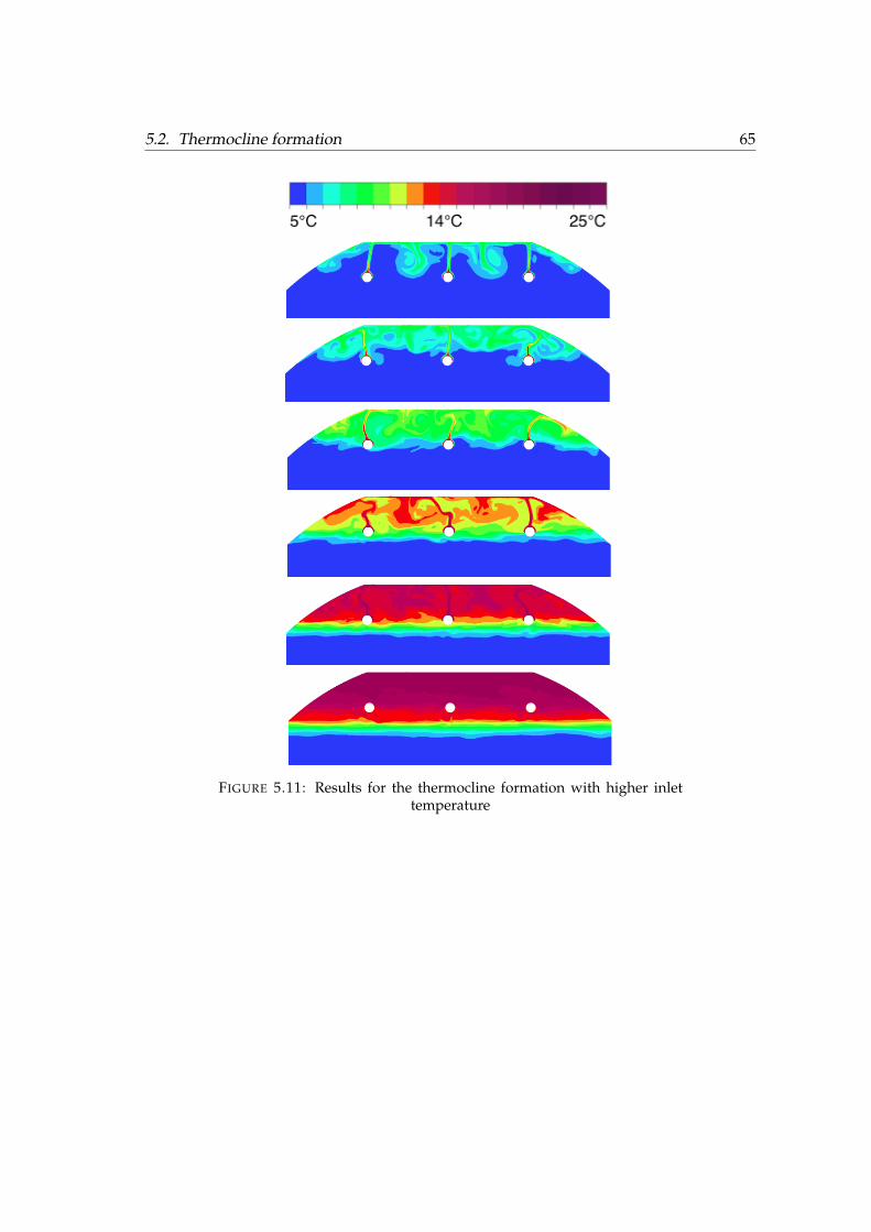
5.2. Thermocline formation 65
FIGURE 5.11: Results for the thermocline formation with higher inlettemperature

66 Chapter 5. Thermocline evolution
278 280 282 284 286 288 290 292
0
5
10
15
Temperature (K)
Tank
heig
ht(m
)
278 279 280 281 282 283 284 285 286 287 2889
10
11
12
13
Temperature (K)
Tank
heig
ht(m
)
FIGURE 5.12: Tank height as a function of temperature
The thermocline thickness is only 1 m at the end of the process, which is a great im-provement. The inlet temperature can be brought down to 14 ◦C when the thermoclinepasses below the upper pipes.
Next, the same type of simulation is conducted with a different geometry: this timewith five distributors. The following pictures show the thermocline formation for out-lets velocities of 1.5 cm/s, from t = 0 min to t = 60 min. The initial temperature of thewater in the cave is 5.7 ◦C and the temperature of the warm water injected water is25 ◦C.
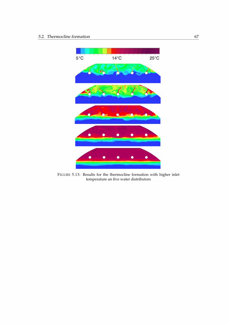
5.2. Thermocline formation 67
FIGURE 5.13: Results for the thermocline formation with higher inlettemperature an five water distributors
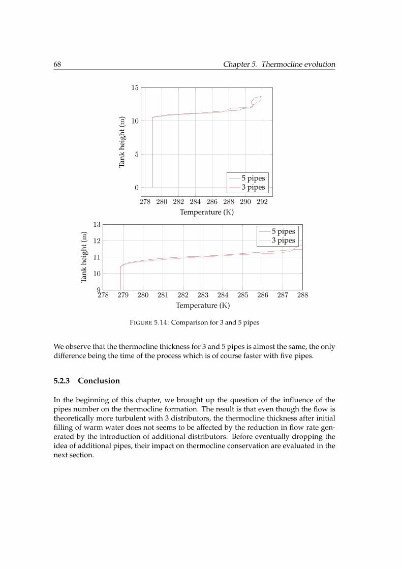
68 Chapter 5. Thermocline evolution
278 280 282 284 286 288 290 292
0
5
10
15
Temperature (K)
Tank
heig
ht(m
)
5 pipes3 pipes
278 279 280 281 282 283 284 285 286 287 2889
10
11
12
13
Temperature (K)
Tank
heig
ht(m
) 5 pipes3 pipes
FIGURE 5.14: Comparison for 3 and 5 pipes
We observe that the thermocline thickness for 3 and 5 pipes is almost the same, the onlydifference being the time of the process which is of course faster with five pipes.
5.2.3 Conclusion
In the beginning of this chapter, we brought up the question of the influence of thepipes number on the thermocline formation. The result is that even though the flow istheoretically more turbulent with 3 distributors, the thermocline thickness after initialfilling of warm water does not seems to be affected by the reduction in flow rate gen-erated by the introduction of additional distributors. Before eventually dropping theidea of additional pipes, their impact on thermocline conservation are evaluated in thenext section.
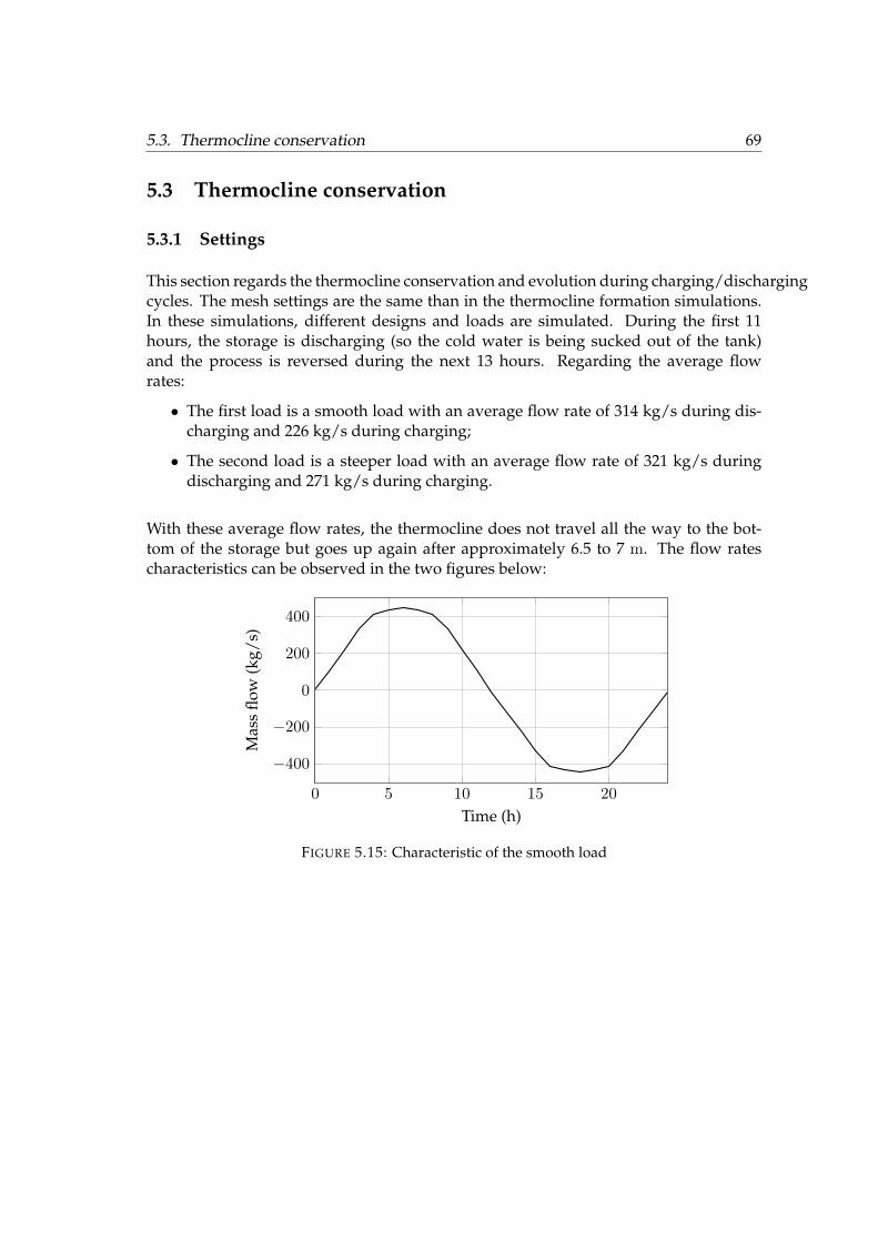
5.3. Thermocline conservation 69
5.3 Thermocline conservation
5.3.1 Settings
This section regards the thermocline conservation and evolution during charging/dischargingcycles. The mesh settings are the same than in the thermocline formation simulations.In these simulations, different designs and loads are simulated. During the first 11hours, the storage is discharging (so the cold water is being sucked out of the tank)and the process is reversed during the next 13 hours. Regarding the average flowrates:
• The first load is a smooth load with an average flow rate of 314 kg/s during dis-charging and 226 kg/s during charging;
• The second load is a steeper load with an average flow rate of 321 kg/s duringdischarging and 271 kg/s during charging.
With these average flow rates, the thermocline does not travel all the way to the bot-tom of the storage but goes up again after approximately 6.5 to 7 m. The flow ratescharacteristics can be observed in the two figures below:
0 5 10 15 20
−400
−200
0
200
400
Time (h)
Mas
sflo
w(k
g/s)
FIGURE 5.15: Characteristic of the smooth load
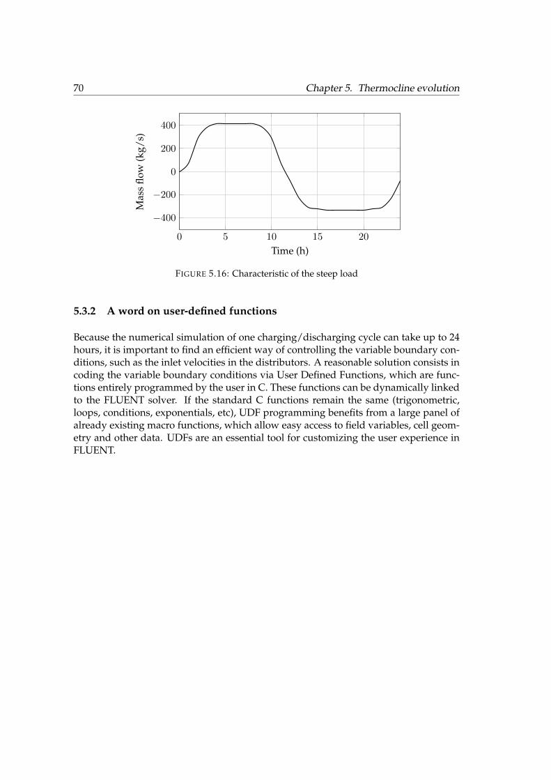
70 Chapter 5. Thermocline evolution
0 5 10 15 20
−400
−200
0
200
400
Time (h)
Mas
sflo
w(k
g/s)
FIGURE 5.16: Characteristic of the steep load
5.3.2 A word on user-defined functions
Because the numerical simulation of one charging/discharging cycle can take up to 24hours, it is important to find an efficient way of controlling the variable boundary con-ditions, such as the inlet velocities in the distributors. A reasonable solution consists incoding the variable boundary conditions via User Defined Functions, which are func-tions entirely programmed by the user in C. These functions can be dynamically linkedto the FLUENT solver. If the standard C functions remain the same (trigonometric,loops, conditions, exponentials, etc), UDF programming benefits from a large panel ofalready existing macro functions, which allow easy access to field variables, cell geom-etry and other data. UDFs are an essential tool for customizing the user experience inFLUENT.
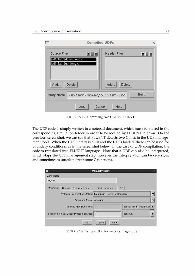
5.3. Thermocline conservation 71
FIGURE 5.17: Compiling two UDF in FLUENT
The UDF code is simply written in a notepad document, which must be placed in thecorresponding simulation folder in order to be located by FLUENT later on. On theprevious screenshot, we can see that FLUENT detects two C files in the UDF manage-ment tools. When the UDF library is built and the UDFs loaded, these can be used forboundary conditions, as in the screenshot below. In the case of UDF compilation, thecode is translated into FLUENT language. Note that a UDF can also be interpreted,which skips the UDF management step, however the interpretation can be very slow,and sometimes is unable to treat some C functions.
FIGURE 5.18: Using a UDF for velocity magnitude
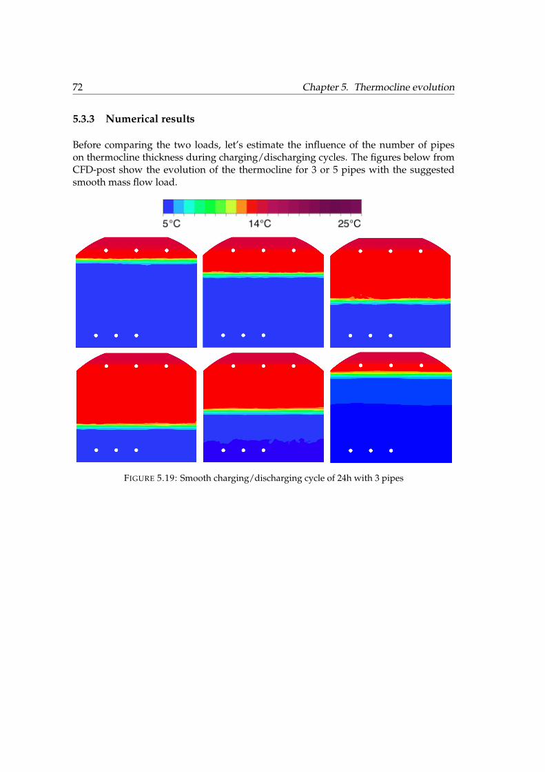
72 Chapter 5. Thermocline evolution
5.3.3 Numerical results
Before comparing the two loads, let’s estimate the influence of the number of pipeson thermocline thickness during charging/discharging cycles. The figures below fromCFD-post show the evolution of the thermocline for 3 or 5 pipes with the suggestedsmooth mass flow load.
FIGURE 5.19: Smooth charging/discharging cycle of 24h with 3 pipes
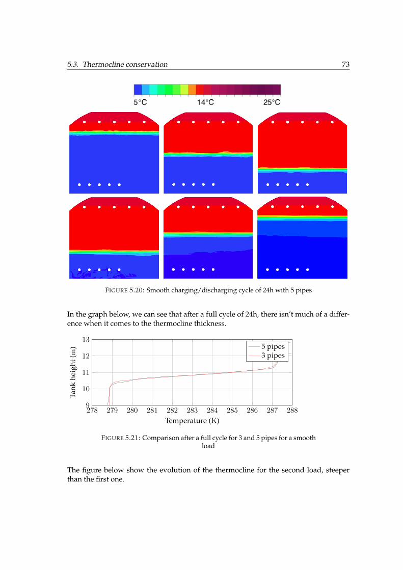
5.3. Thermocline conservation 73
FIGURE 5.20: Smooth charging/discharging cycle of 24h with 5 pipes
In the graph below, we can see that after a full cycle of 24h, there isn’t much of a differ-ence when it comes to the thermocline thickness.
278 279 280 281 282 283 284 285 286 287 2889
10
11
12
13
Temperature (K)
Tank
heig
ht(m
) 5 pipes3 pipes
FIGURE 5.21: Comparison after a full cycle for 3 and 5 pipes for a smoothload
The figure below show the evolution of the thermocline for the second load, steeperthan the first one.
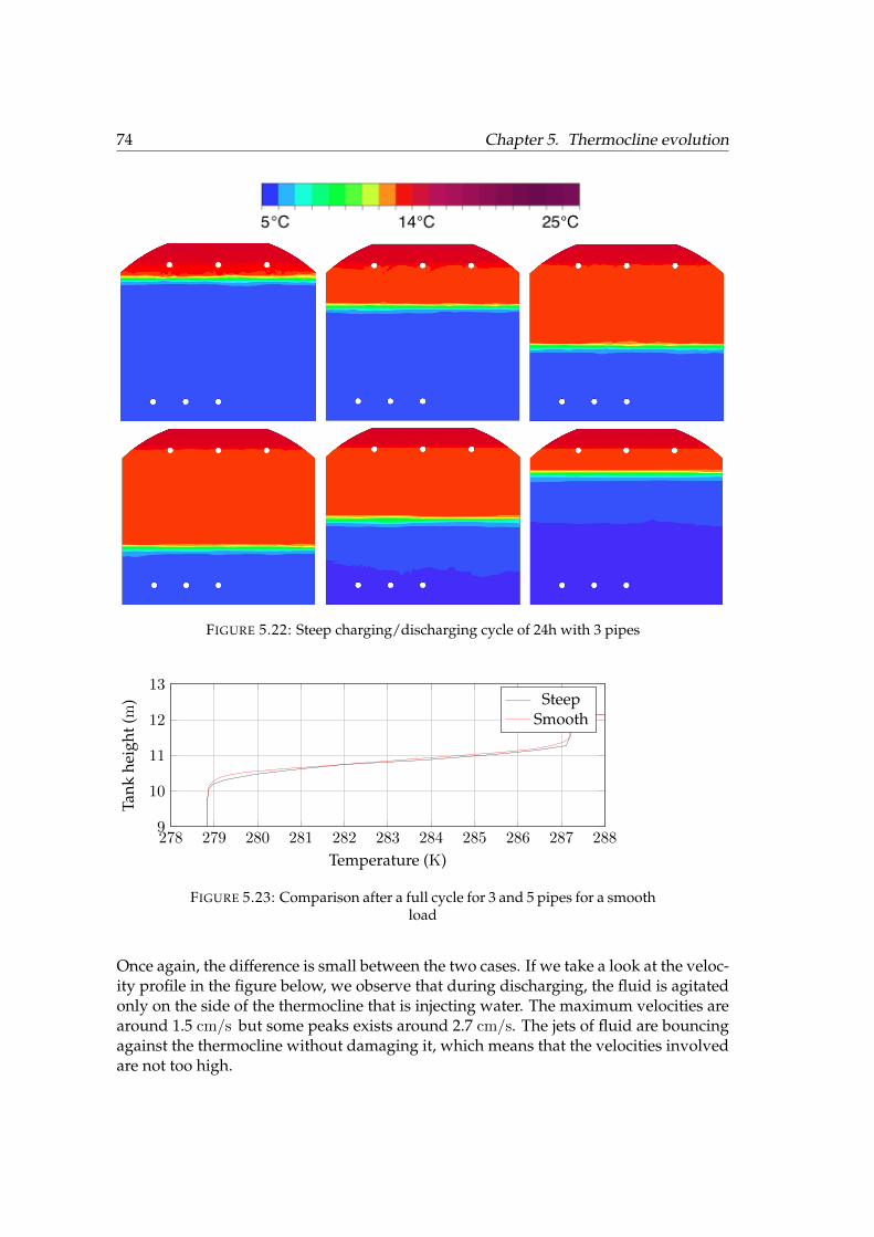
74 Chapter 5. Thermocline evolution
FIGURE 5.22: Steep charging/discharging cycle of 24h with 3 pipes
278 279 280 281 282 283 284 285 286 287 2889
10
11
12
13
Temperature (K)
Tank
heig
ht(m
) SteepSmooth
FIGURE 5.23: Comparison after a full cycle for 3 and 5 pipes for a smoothload
Once again, the difference is small between the two cases. If we take a look at the veloc-ity profile in the figure below, we observe that during discharging, the fluid is agitatedonly on the side of the thermocline that is injecting water. The maximum velocities arearound 1.5 cm/s but some peaks exists around 2.7 cm/s. The jets of fluid are bouncingagainst the thermocline without damaging it, which means that the velocities involvedare not too high.

5.3. Thermocline conservation 75
FIGURE 5.24: Velocity magnitude during discharging
5.3.4 Thickness evolution for several cycles
The figures and graphs below present the evolution of the thermocline thickness forsix cycles of 24 hours. This simulation was the most time consuming, with 9 days ofcalculations.
FIGURE 5.25: Thermocline evolution for 6 days of charging/discharging(days 2, 4, 6)
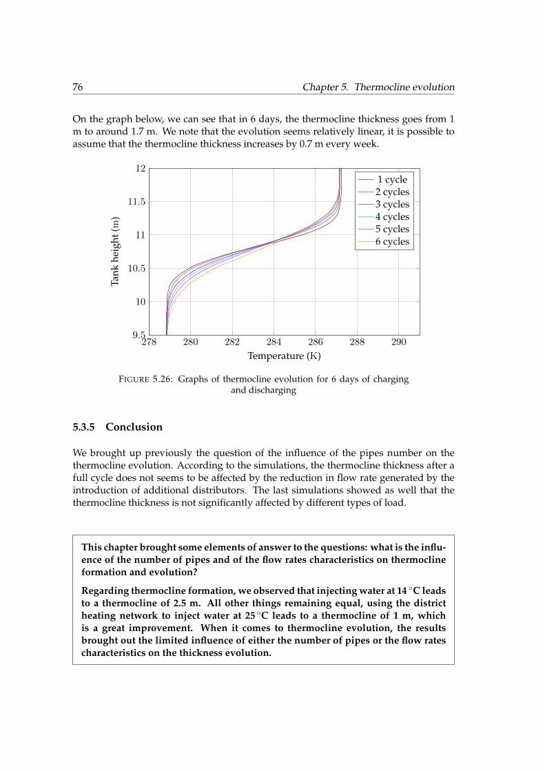
76 Chapter 5. Thermocline evolution
On the graph below, we can see that in 6 days, the thermocline thickness goes from 1m to around 1.7 m. We note that the evolution seems relatively linear, it is possible toassume that the thermocline thickness increases by 0.7 m every week.
278 280 282 284 286 288 2909.5
10
10.5
11
11.5
12
Temperature (K)
Tank
heig
ht(m
)
1 cycle2 cycles3 cycles4 cycles5 cycles6 cycles
FIGURE 5.26: Graphs of thermocline evolution for 6 days of chargingand discharging
5.3.5 Conclusion
We brought up previously the question of the influence of the pipes number on thethermocline evolution. According to the simulations, the thermocline thickness after afull cycle does not seems to be affected by the reduction in flow rate generated by theintroduction of additional distributors. The last simulations showed as well that thethermocline thickness is not significantly affected by different types of load.
This chapter brought some elements of answer to the questions: what is the influ-ence of the number of pipes and of the flow rates characteristics on thermoclineformation and evolution?
Regarding thermocline formation, we observed that injecting water at 14 ◦C leadsto a thermocline of 2.5 m. All other things remaining equal, using the districtheating network to inject water at 25 ◦C leads to a thermocline of 1 m, whichis a great improvement. When it comes to thermocline evolution, the resultsbrought out the limited influence of either the number of pipes or the flow ratescharacteristics on the thickness evolution.
77
Chapter 6
Stratification characterization andconclusion
6.1 Richardson and MIX numbers
The Richardson number has been suggested in the second chapter. It relates the ratiobetween the gravitational potential energy of a fluid particle and its kinetic energy. Or,in other words, it is the ratio of the buoyancy forces and the mixing forces, or natu-ral convection and forced convection. A Richardson number smaller than 1 indicatesa flow governed by forced convection. A larger Richardson number indicates a strat-ified storage. With β being the thermal expansion coefficient of the fluid and ∆T thetemperature difference of the fluid considered:
Ri =gβ∆Td
v2(6.1)
We can calculate the Richardson number for a useful height of d = 7 m, a thermalexpansion coefficient of β = 8.8 × 10⁵, a ∆T = 10 K and a characteristic speed of 2 cmper second.
Ri =9.81× 8.8× 105 × 10× 7
0.022= 151
This result indicates that the storage is strongly stratified. We can also find the theo-retical value for which the Richardson number equals 1, which means that the forcedconvection start to takes over the natural convection. We find Ri = 1 for v = 25cm/s.A Richardson number of 10 is found for a characteristic speed around 8 cm/s. Stayingbelow 8 cm/s at the distributors outlets theoretically ensures that mixing forces will notbe an obstacle to stratification.
Another number that can be used to characterize stratification is the MIX number,which was defined by Andersen et al.[25]. The MIX number is based on the temper-ature distribution in the tank and it is determined by the first moment of energy. In
78 Chapter 6. Stratification characterization and conclusion
other words, the stratification is characterized by the energy in the storage, weightedby vertical location. The MIX number is defined as follow:
MIX =ME,stratified −ME,actual
ME,stratified −ME,fully−mixed(6.2)
where ME are the first moments of energy defined as:
ME =
n∑i=1
yi.Ei (6.3)
with Ei the energy contained in the strate i expressed as:
Ei = ρ.Vi.Cp.Ti (6.4)
The MIX number goes from 0 to 1, 0 representing a perfectly stratified storage. We cancalculate the MIX number from our simulation. The vertical height is defined such asthe bottom of the cave is 0 (then the top distributors are at 12 m). First, the levels ofenergy Ei are defined for a perfectly stratified storage, for different discharging times.We define here a non dimensional time from t = 0 to t = 1, which represents the entireduration of the discharging process. The calculations are done with the values obtainedin the last simulation of the previous chapter, for the first discharging cycle.
After defining strates of 1 meter, we obtain for the warm strates:
Ewarm = ρ.V.Cp.Twarm = 2.44× 10¹² J
Similarly, for the cold strates:
Ecold = ρ.V.Cp.Tcold = 2.37× 10¹² J
We can then calculate the first moment of energy for a perfectly stratified storage fordifferent times.
TABLE 6.1: First moment of energy for a perfectly stratified tank
t 0 0.25 0.5 0.75 1
ME,stratified(1014) 1.712 1.726 1.737 1.746 1.752
Then the moments of energy are calculated for the actual storage, with the simulationresults.
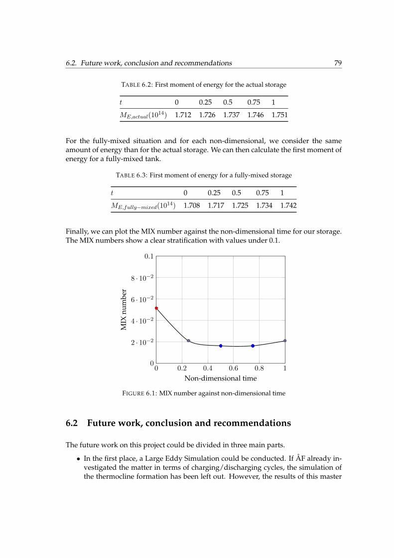
6.2. Future work, conclusion and recommendations 79
TABLE 6.2: First moment of energy for the actual storage
t 0 0.25 0.5 0.75 1
ME,actual(1014) 1.712 1.726 1.737 1.746 1.751
For the fully-mixed situation and for each non-dimensional, we consider the sameamount of energy than for the actual storage. We can then calculate the first moment ofenergy for a fully-mixed tank.
TABLE 6.3: First moment of energy for a fully-mixed storage
t 0 0.25 0.5 0.75 1
ME,fully−mixed(1014) 1.708 1.717 1.725 1.734 1.742
Finally, we can plot the MIX number against the non-dimensional time for our storage.The MIX numbers show a clear stratification with values under 0.1.
0 0.2 0.4 0.6 0.8 10
2 · 10−2
4 · 10−2
6 · 10−2
8 · 10−2
0.1
Non-dimensional time
MIX
num
ber
FIGURE 6.1: MIX number against non-dimensional time
6.2 Future work, conclusion and recommendations
The future work on this project could be divided in three main parts.
• In the first place, a Large Eddy Simulation could be conducted. If ÅF already in-vestigated the matter in terms of charging/discharging cycles, the simulation ofthe thermocline formation has been left out. However, the results of this master
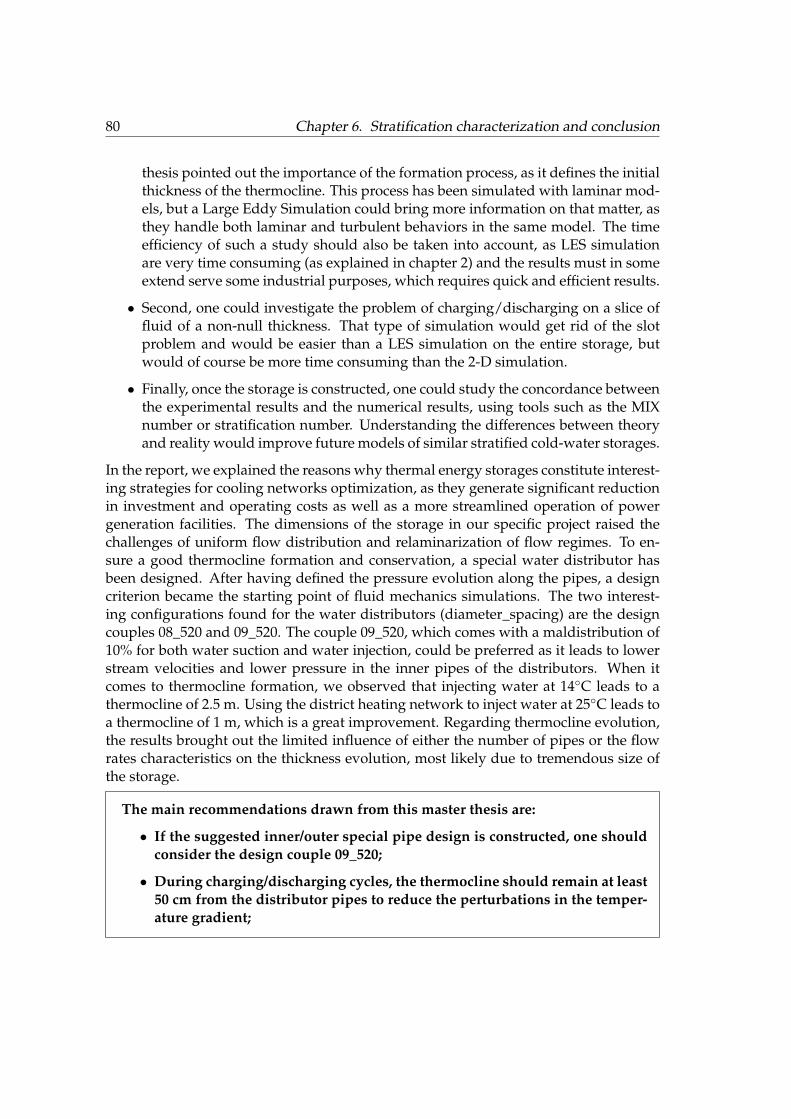
80 Chapter 6. Stratification characterization and conclusion
thesis pointed out the importance of the formation process, as it defines the initialthickness of the thermocline. This process has been simulated with laminar mod-els, but a Large Eddy Simulation could bring more information on that matter, asthey handle both laminar and turbulent behaviors in the same model. The timeefficiency of such a study should also be taken into account, as LES simulationare very time consuming (as explained in chapter 2) and the results must in someextend serve some industrial purposes, which requires quick and efficient results.
• Second, one could investigate the problem of charging/discharging on a slice offluid of a non-null thickness. That type of simulation would get rid of the slotproblem and would be easier than a LES simulation on the entire storage, butwould of course be more time consuming than the 2-D simulation.
• Finally, once the storage is constructed, one could study the concordance betweenthe experimental results and the numerical results, using tools such as the MIXnumber or stratification number. Understanding the differences between theoryand reality would improve future models of similar stratified cold-water storages.
In the report, we explained the reasons why thermal energy storages constitute interest-ing strategies for cooling networks optimization, as they generate significant reductionin investment and operating costs as well as a more streamlined operation of powergeneration facilities. The dimensions of the storage in our specific project raised thechallenges of uniform flow distribution and relaminarization of flow regimes. To en-sure a good thermocline formation and conservation, a special water distributor hasbeen designed. After having defined the pressure evolution along the pipes, a designcriterion became the starting point of fluid mechanics simulations. The two interest-ing configurations found for the water distributors (diameter_spacing) are the designcouples 08_520 and 09_520. The couple 09_520, which comes with a maldistribution of10% for both water suction and water injection, could be preferred as it leads to lowerstream velocities and lower pressure in the inner pipes of the distributors. When itcomes to thermocline formation, we observed that injecting water at 14◦C leads to athermocline of 2.5 m. Using the district heating network to inject water at 25◦C leads toa thermocline of 1 m, which is a great improvement. Regarding thermocline evolution,the results brought out the limited influence of either the number of pipes or the flowrates characteristics on the thickness evolution, most likely due to tremendous size ofthe storage.
The main recommendations drawn from this master thesis are:
• If the suggested inner/outer special pipe design is constructed, one shouldconsider the design couple 09_520;
• During charging/discharging cycles, the thermocline should remain at least50 cm from the distributor pipes to reduce the perturbations in the temper-ature gradient;

6.2. Future work, conclusion and recommendations 81
• To monitor the evolution of the thermocline, some temperature sensorscould be placed at different locations, both far and close to the walls, andwith vertical spacings of at least less than 1m to capture the evolution ofthe thermocline.

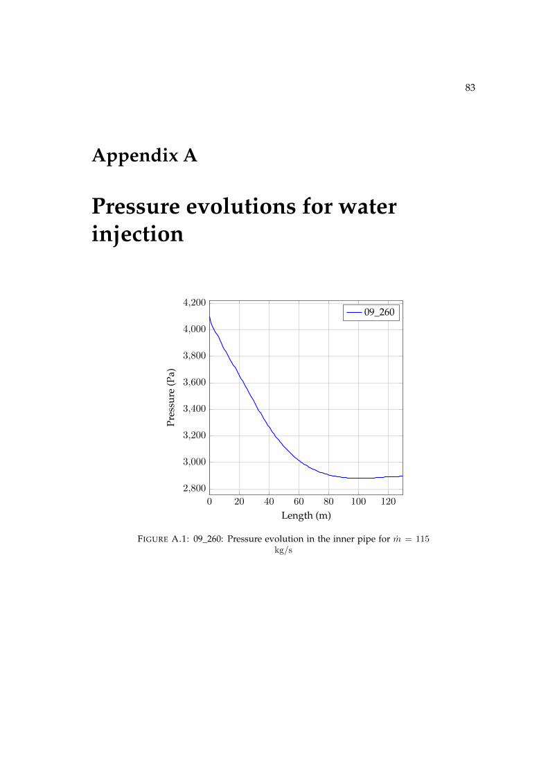
83
Appendix A
Pressure evolutions for waterinjection
0 20 40 60 80 100 120
2,800
3,000
3,200
3,400
3,600
3,800
4,000
4,200
Length (m)
Pres
sure
(Pa)
09_260
FIGURE A.1: 09_260: Pressure evolution in the inner pipe for m = 115kg/s
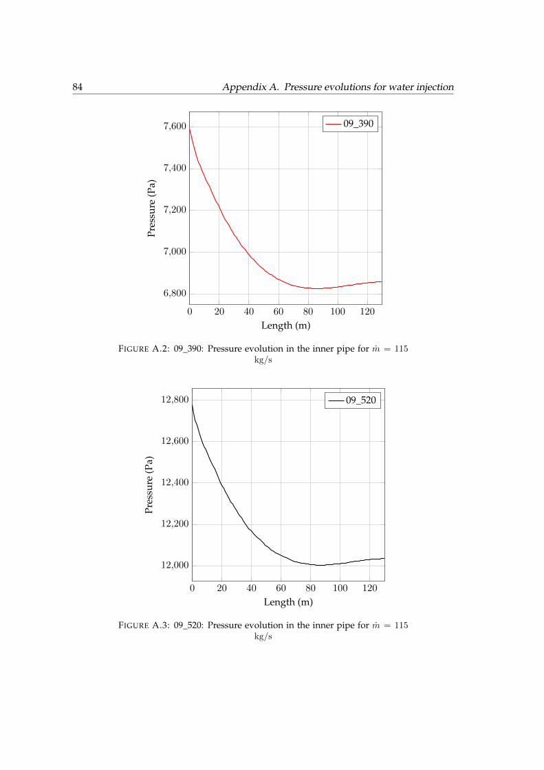
84 Appendix A. Pressure evolutions for water injection
0 20 40 60 80 100 120
6,800
7,000
7,200
7,400
7,600
Length (m)
Pres
sure
(Pa)
09_390
FIGURE A.2: 09_390: Pressure evolution in the inner pipe for m = 115kg/s
0 20 40 60 80 100 120
12,000
12,200
12,400
12,600
12,800
Length (m)
Pres
sure
(Pa)
09_520
FIGURE A.3: 09_520: Pressure evolution in the inner pipe for m = 115kg/s
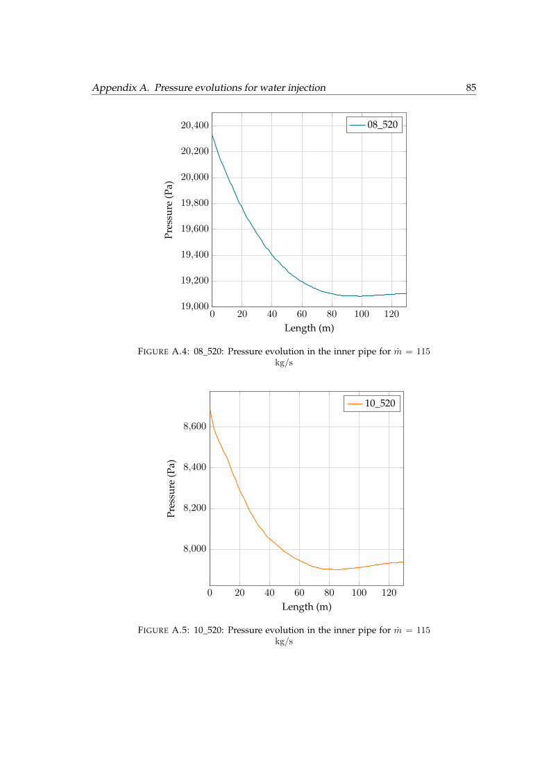
Appendix A. Pressure evolutions for water injection 85
0 20 40 60 80 100 12019,000
19,200
19,400
19,600
19,800
20,000
20,200
20,400
Length (m)
Pres
sure
(Pa)
08_520
FIGURE A.4: 08_520: Pressure evolution in the inner pipe for m = 115kg/s
0 20 40 60 80 100 120
8,000
8,200
8,400
8,600
Length (m)
Pres
sure
(Pa)
10_520
FIGURE A.5: 10_520: Pressure evolution in the inner pipe for m = 115kg/s

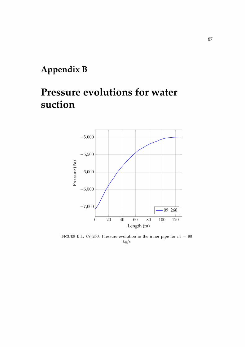
87
Appendix B
Pressure evolutions for watersuction
0 20 40 60 80 100 120
−7,000
−6,500
−6,000
−5,500
−5,000
Length (m)
Pres
sure
(Pa)
09_260
FIGURE B.1: 09_260: Pressure evolution in the inner pipe for m = 90kg/s
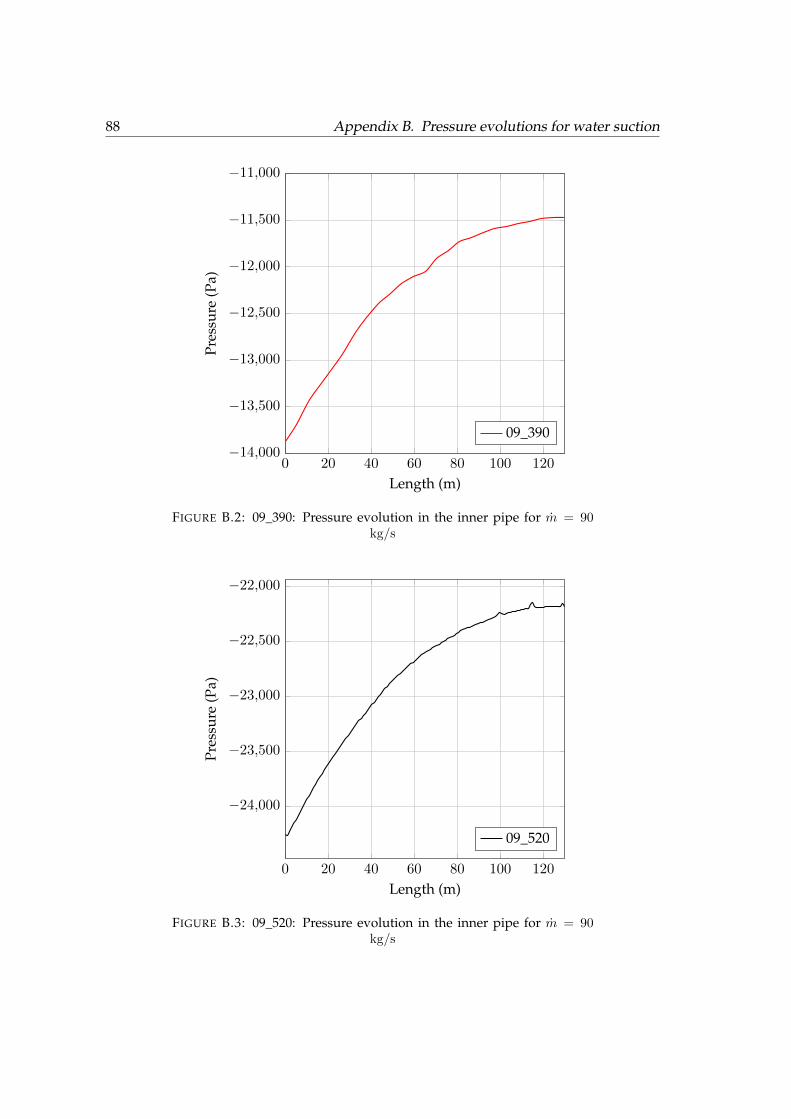
88 Appendix B. Pressure evolutions for water suction
0 20 40 60 80 100 120−14,000
−13,500
−13,000
−12,500
−12,000
−11,500
−11,000
Length (m)
Pres
sure
(Pa)
09_390
FIGURE B.2: 09_390: Pressure evolution in the inner pipe for m = 90kg/s
0 20 40 60 80 100 120
−24,000
−23,500
−23,000
−22,500
−22,000
Length (m)
Pres
sure
(Pa)
09_520
FIGURE B.3: 09_520: Pressure evolution in the inner pipe for m = 90kg/s
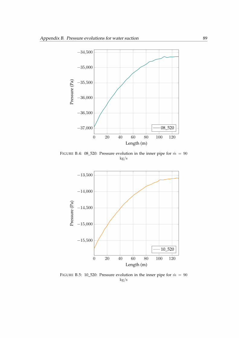
Appendix B. Pressure evolutions for water suction 89
0 20 40 60 80 100 120
−37,000
−36,500
−36,000
−35,500
−35,000
−34,500
Length (m)
Pres
sure
(Pa)
08_520
FIGURE B.4: 08_520: Pressure evolution in the inner pipe for m = 90kg/s
0 20 40 60 80 100 120
−15,500
−15,000
−14,500
−14,000
−13,500
Length (m)
Pres
sure
(Pa)
10_520
FIGURE B.5: 10_520: Pressure evolution in the inner pipe for m = 90kg/s

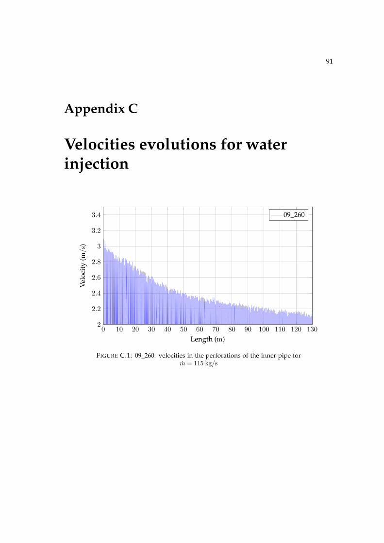
91
Appendix C
Velocities evolutions for waterinjection
0 10 20 30 40 50 60 70 80 90 100 110 120 1302
2.2
2.4
2.6
2.8
3
3.2
3.4
Length (m)
Velo
city
(m/s)
09_260
FIGURE C.1: 09_260: velocities in the perforations of the inner pipe form = 115 kg/s
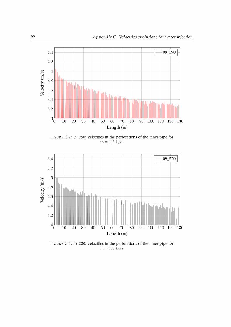
92 Appendix C. Velocities evolutions for water injection
0 10 20 30 40 50 60 70 80 90 100 110 120 1303
3.2
3.4
3.6
3.8
4
4.2
4.4
Length (m)
Velo
city
(m/s
)
09_390
FIGURE C.2: 09_390: velocities in the perforations of the inner pipe form = 115 kg/s
0 10 20 30 40 50 60 70 80 90 100 110 120 1304
4.2
4.4
4.6
4.8
5
5.2
5.4
Length (m)
Velo
city
(m/s
)
09_520
FIGURE C.3: 09_520: velocities in the perforations of the inner pipe form = 115 kg/s

Appendix C. Velocities evolutions for water injection 93
0 10 20 30 40 50 60 70 80 90 100 110 120 1305
5.2
5.4
5.6
5.8
6
6.2
Length (m)
Velo
city
(m/s)
08_520
FIGURE C.4: 08_520: velocities in the perforations of the inner pipe form = 115 kg/s
0 10 20 30 40 50 60 70 80 90 100 110 120 1303
3.2
3.4
3.6
3.8
4
4.2
4.4
Length (m)
Velo
city
(m/s)
10_520
FIGURE C.5: 10_520: velocities in the perforations of the inner pipe form = 115 kg/s

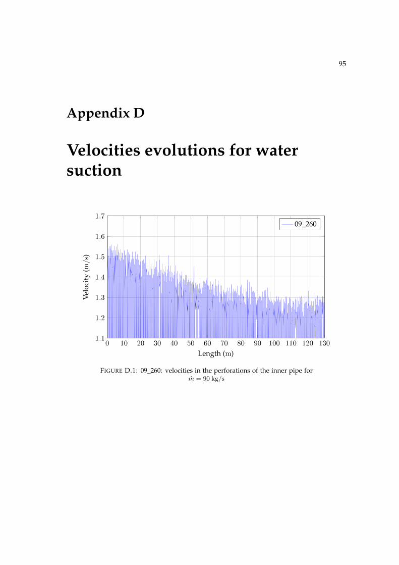
95
Appendix D
Velocities evolutions for watersuction
0 10 20 30 40 50 60 70 80 90 100 110 120 1301.1
1.2
1.3
1.4
1.5
1.6
1.7
Length (m)
Velo
city
(m/s)
09_260
FIGURE D.1: 09_260: velocities in the perforations of the inner pipe form = 90 kg/s

96 Appendix D. Velocities evolutions for water suction
0 10 20 30 40 50 60 70 80 90 100 110 120 1301.7
1.8
1.9
2
2.1
2.2
2.3
2.4
Length (m)
Velo
city
(m/s
)
09_390
FIGURE D.2: 09_390: velocities in the perforations of the inner pipe form = 90 kg/s
0 10 20 30 40 50 60 70 80 90 100 110 120 1302.5
2.6
2.7
2.8
2.9
3
Length (m)
Velo
city
(m/s
)
09_520
FIGURE D.3: 09_520: velocities in the perforations of the inner pipe form = 90 kg/s
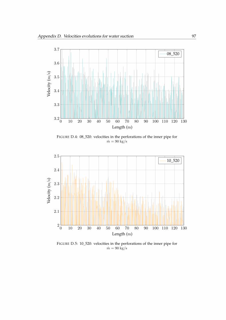
Appendix D. Velocities evolutions for water suction 97
0 10 20 30 40 50 60 70 80 90 100 110 120 1303.2
3.3
3.4
3.5
3.6
3.7
Length (m)
Velo
city
(m/s)
08_520
FIGURE D.4: 08_520: velocities in the perforations of the inner pipe form = 90 kg/s
0 10 20 30 40 50 60 70 80 90 100 110 120 1302
2.1
2.2
2.3
2.4
2.5
Length (m)
Velo
city
(m/s)
10_520
FIGURE D.5: 10_520: velocities in the perforations of the inner pipe form = 90 kg/s

99
Bibliography
[1] S. Electric, “Overview of the group’s strategy, markets and businesses,” 2015.
[2] Fjärrvärme, “What is district cooling.”
[3] I. D. E. Association, “Idea report: The district energy industry,” tech. rep., 2015.
[4] N. G. News, “The ac of tomorrow: Tapping deep water for cooling.”
[5] D. Energy, “Dream city: Air conditioning is a public good,” 2013.
[6] “Slideshare on reciprocating compressors.”
[7] “Air compressor guide.”
[8] “Youtube video.”
[9] M. Rouleau, “Chilled water thermal energy storage: an alternative to static ice analternative to static ice,” tech. rep., FEFPA, 2015.
[10] J. DELBES, “Réseaux de froid urbain,” tech. rep., Techniques de l’ingénieur, janvier2000.
[11] M. R. Ibrahim Dincer, Thermal Energy Storage: Systems and Applications. 2002.
[12] C. Wollblad, “Simulering av flode i fjarrkyllager,” tech. rep., AF, 2015.
[13] W. Frei, “Which turbulence model should i choose for my cfd application,” 2013.
[14] M. M. A. Castell, “Dimensionless numbers used to characterize stratification inwater tanks for discharging at low flow rates,” Renewable Energy: An InternationalJournal, no. 35, 2010.
[15] A. J. Chorin, “Vorticity and turbulence,” Applied Mathematical Sciences, vol. 103,1994.
[16] S. A. Orszag, “Analytical theories of turbulence,” Journal of Fluid Mechanics, vol. 41,pp. 363–386, 1970.
[17] K. Gersten, Boundary-layer Theory. Springer, 8th revised ed. ed., 2000.
[18] “Wikipedia article on law of the wall.”
[19] “Wikipedia article on law of the wall.”
[20] ANSYS Fluent 12.0 User’s Guide. 2009.
100 BIBLIOGRAPHY
[21] V. E. Senecal, “Fluid distribution in process equipment,” Fluid mechanics in chemicalengineering, 1957.
[22] A. J. McLemore, “A study of discharge coefficients for orifices cut into roundpipes,” Journal of Irrigation and Drainage Engineering, August 2013.
[23] J. N. Tilton, Perry’s Chemical Engineers’ Handbook, section 6. 8th ed., 2008.
[24] A. K. Majid Farajpourlar, Jidon Janaun, “Gas flow through vertical pipe and per-forated vertical pipe,” International Journal of ChemTech Research, vol. 7, no. 6,pp. 2589–2595, 2015.
[25] F. J. Andersen E, Furbo S, “Multilayer fabric stratification pipes for solar tanks,”Solar Energy, vol. 81, pp. 1219–1226, 2007.