Numerical Solutions of singular Two Point BVPsNumerical Solution of Singular Two Point BVPs J.Cash,...

ASC Report No. 22/2008

Numerical Solutions of singular Two PointBVPs

Jeff Cash, Georg Kitzhofer, Othmar Koch, Gerald Moore, Ewa

Weinmuller

Institute for Analysis and Scientific Computing

Vienna University of Technology — TU Wien

www.asc.tuwien.ac.at ISBN 978-3-902627-00-1

Most recent ASC Reports

21/2008 Samuel Ferraz-Leite, Dirk PraetoriusA Posteriori Fehlerschatzer fur die Symmsche Integralgleichung in 3D

20/2008 Bertram DuringAsset Pricing under Information with Stochastic Volatility

19/2008 Stefan Funken, Dirk Praetorius, Philipp WissgottEfficient Implementation of Adaptive P1-FEM in MATLAB

18/2008 Bertram During, Guiseppe ToscaniInternational and Domestic Trading and Wealth Distribution

17/2008 Vyacheslav Pivovarchik, Harald WoracekSums of Nevanlinna Functions and Differential Equations on Star-Shaped Gra-phs

16/2008 Bertram During, Daniel Matthes, Guiseppe ToscaniKinetic Equations Modelling Wealth Redistribution: A Comparison of Approa-ches

15/2008 Jens Markus Melenk, Stefan SauterConvergence Analysis for Finite Element Discretizations of the Helmholtz Equa-tion. Part I: the Full Space Problem

14/2008 Anton Arnold, Francao Fagnola, Lukas NeumannQuantum Fokker-Planck Models: the Lindblad and Wigner Approaches

13/2008 Jingzhi Li, Jens Markus Melenk, Barbara Wohlmuth, Jun ZouOptimal Convergence of Higher Order Finite Element Methods for Elliptic In-terface Problems

12/2008 Samuel Ferraz-Leite, Christoph Ortner, Dirk PraetoriusAdaptive Boundary Element Method:Simple Error Estimators and Convergence

Institute for Analysis and Scientific ComputingVienna University of TechnologyWiedner Hauptstraße 8–101040 Wien, Austria

E-Mail: [email protected]

WWW: http://www.asc.tuwien.ac.at

FAX: +43-1-58801-10196

ISBN 978-3-902627-00-1

c© Alle Rechte vorbehalten. Nachdruck nur mit Genehmigung des Autors.

ASCTU WIEN

Numerical Solution of Singular Two Point BVPs

J.Cash, G. Kitzhofer, O.Koch, G.Moore, E.Weinmuller

July 8, 2008

Abstract

An algorithm is described for the efficient numerical solution of singular two-point boundary value prob-lems. The algorithm is based on collocation at Gauss points, is applied directly to second order equationsand uses a transformation of the independent variable to obtain extra smoothness if needed. Numericalcomparisons between a code based on this approach and codes based on other options which have pre-viously been thought of as possible alternatives such as collocation at Lobatto points or reduction to afirst order system, are made and the efficiency of the new approach is clearly demonstrated by numericalresults.

1 Introduction

Mathematical models of classical applications from physics, chemistry and mechanics (e.g. the Thomas–Fermi differential equation, the Ginzburg–Landau equation) take the form of singular boundary valueproblems of second order: the singularity typically occurring at an end of the interval of integration.ODEs with singularities appear also in numerous applications which are of interest in modern appliedmathematics. Computations of self-similar blow-up solutions of nonlinear PDEs lead to the computationof problems from this class ([7], [8], [9], [10], [11]). Also, the density profile equation in hydrodynamicsmay be reduced to a singular ODE ([24], [29]). Finally, the investigation of problems in the theory ofshallow membrane caps, [35], is associated with such problems. Even in ecology, in the computation ofavalanche run-up, this problem class is present ([27], [32]). Further research areas include the solutionof differential equations posed on unbounded intervals ([1], [10] and [16]), the computation of connectingorbits or invariant manifolds for dynamical systems ([33] and [34]), differential-algebraic equations ([31]) orSturm–Liouville eigenvalue problems ([14], and [30]). Hence several papers are concerned with numericalmethods for approximating such problems, cf. [12], [15], [17], [22].

The aim of the present paper is to give a comprehensive assessment of the performance of somestandard collocation algorithms, when applied to singular boundary value problems: in particular wecompare numerical results for both first and second order formulations of the same singular boundaryvalue problem and compare both Gauss and Lobatto collocation algorithms. Collocation at Lobattopoints needs special consideration for singular boundary value problems, because then we need to collocateat the singular end-point. We also consider how a suitable transformation of the independent variablecan affect the performance of our collocation algorithms. Again, this is especially important for singularboundary value problems, because such a transformation alters key eigenvalues and may increase thesmoothness of our solution and consequently, the performance of numerical solution methods. Concerningsoftware, there are some possibilities to use open domain codes to treat singular boundary value problems,cf. Section 4, but we do not intend to compare these codes here. This is an interesting but difficult questionand it will be addressed in an upcoming paper.

The contents of the present paper are as follows. In Section 2 we briefly state the basic analyticalproperties of singular boundary value problems with a singularity of the first kind, for both first andsecond order systems. We emphasise how the number of boundary conditions required for a well-posed

1

problem depends on certain eigenvalue conditions. We also show how a transformation of the independentvariable alters these eigenvalue conditions, and may also alter the smoothness of our solutions. In Section 3we discuss how collocation algorithms can be applied to approximate the solution of singular boundaryvalue problems, both for first order and second order systems. We emphasise how the implicit boundaryconditions in the continuous formulation must be made explicit in order to construct a well-posed discreteproblem. We also discuss how to collocate at the singular end-point, when a Lobatto algorithm is used.Finally, we show how to transform from second order singular systems to corresponding first order singularsystems, in a manner which maintains the structure of the boundary value problem. We describe themodel problems that we use in Section 4, and display some numerical results in Section 5. Based onthe extensive numerical testing that we have done, we recommend an algorithm which uses collocationon Gauss points, which uses variable stepsize to control the error, is applied directly to second orderproblems and which uses a transformation of the independent variable to obtain extra smoothness ifneeded. We expect that our code based on this approach will be very competitive with the best existingcodes and we will investigate this in detail in future work.

2 Analytical Results for Singular Problems

In this section we will briefly recapitulate some of the analytical properties of singular systems of firstand second order boundary value problems. For more details, we refer to [20] for the former and [40] forthe latter.

2.1 Singular first order systems

We consider the nonlinear ODE

y′(t) − M

ty(t) = f(t,y(t)) 0 < t ≤ 1 (2.1)

with boundary conditionsb(y(0),y(1)) = 0, (2.2)

where y : [0, 1] 7→ Rn, M ∈ R

n×n, f : [0, 1]×Rn 7→ R

n and b : Rn×R

n 7→ Rp with the value of p discussed

below. We shall be seeking a solution y⋆ ∈ C[0, 1] ∩ C1(0, 1] and so we assume that f is continuous withrespect to its first argument and continuously differentiable with respect to its second. Also b is assumedto be continuously differentiable with respect to its arguments.

The most important consideration for the matrix M is the sign of the real part of its eigenvalues. Wemust have p = n++n0 for a well-posed problem, where n+ is the dimension of the invariant subspace of M

corresponding to those eigenvalues with strictly positive real part (i.e. combined algebraic multiplicities)and n0 is the dimension of the null-space of M (i.e. geometric multiplicity of the zero eigenvalue). This isbecause the assumption that y⋆ is continuous at t = 0 implicitly provides n− (n+ +n0) initial conditions.

We assume that we are trying to approximate a solution y⋆ which is isolated, i.e. the linear problem

y′(t) − M

ty(t) + N(t)y(t) = 0 0 < t ≤ 1

B0y(0) + B1y(1) = 0

has only the trivial solution in C[0, 1]∩C1(0, 1], where N(t) is the n×n Jacobian matrix of f with respectto its second argument, evaluated at (t,y⋆(t)), B0 is the n × n Jacobian matrix of b with respect to itsfirst argument, evaluated at (y⋆(0),y⋆(1)) and B1 is the n × n Jacobian matrix of b with respect to itssecond argument, evaluated at (y⋆(0),y⋆(1)).

The smoothness of y⋆ depends on the smoothness of f and the positive real parts of eigenvalues of M,e.g. when, for s ≥ 0, f has s continuous derivatives and no eigenvalue of M has real part in (0, s+1], then

2

we must have y⋆ ∈ Cs+1[0, 1], see [20]. The influence of these key eigenvalues of M may be mitigated bya change of independent variable: i.e. if we set

t = τγ

for some γ > 1, then y⋆(τ) ≡ y⋆(τγ) satisfies

y′(τ) − M

τy(τ) = f(τ,y(τ)), 0 < τ ≤ 1, (2.3)

whereM ≡ γM and f(τ,x) ≡ γτγ−1f(τγ ,x),

and the boundary conditions (2.2). Thus the eigenvalues of M are multiplied by γ compared to theeigenvalues of M and so y⋆ can be smoother than y⋆.

2.2 Singular second order systems

We consider the nonlinear ODE

z′′(t) − A1

tz′(t) − A0

t2z(t) = g(t, z(t)) 0 < t ≤ 1 (2.4)

with boundary conditionsc(z(0), z(1), z′(1)) = 0, (2.5)

where z : [0, 1] 7→ Rn, A0, A1 ∈ R

n×n, g : [0, 1] × Rn 7→ R

n and c : Rn × R

n × Rn 7→ R

p with the valueof p discussed below. We shall be seeking a solution z⋆ ∈ C[0, 1] ∩ C2(0, 1] and so we assume that g iscontinuous with respect to its first argument and continuously differentiable with respect to its second.Also c is assumed to be continuously differentiable with respect to its arguments.

The important consideration for the matrices A0 and A1 is the quadratic eigenvalue problem

det(λ2I − λ[I + A1] − A0

)= 0, (2.6)

see [18]. We must have p = n++n0 for a well-posed problem, where n+ is the number of roots (counted inmultiplicity) with strictly positive real part of the 2nth degree polynomial in (2.6) and n0 is the dimensionof the null-space of A0 (i.e. geometric multiplicity of the zero eigenvalue). This is because the assumptionthat z⋆ is continuous at t = 0 implicitly provides 2n − (n+ + n0) initial conditions.

We assume that we are trying to approximate a solution z⋆ which is isolated, i.e. the linear problem

z′′(t) − A1

tz′(t) − A0

t2z(t) − A(t)z(t) = 0 0 < t ≤ 1

C0z(0) + C1z(1) + C′1z

′(1) = 0

has only the trivial solution in C[0, 1]∩C2(0, 1], where A(t) is the n×n Jacobian matrix of g with respectto its second argument, evaluated at (t, z⋆(t)), C0 is the n × n Jacobian matrix of c with respect to itsfirst argument, evaluated at (z⋆(0), z⋆(1), z⋆′(1)), C1 is the n×n Jacobian matrix of c with respect to itssecond argument, evaluated at (z⋆(0), z⋆(1), z⋆′(1)) and C′

1 is the n×n Jacobian matrix of c with respectto its third argument, evaluated at (z⋆(0), z⋆(1), z⋆′(1)).

The smoothness of z⋆ depends on the smoothness of g and the positive real parts of the roots of (2.6),e.g. when, for s ≥ 0, g has s continuous derivatives and no root of (2.6) has real part in (0, s + 2], thenwe must have z⋆ ∈ Cs+2[0, 1], see [40]. The influence of these key roots of (2.6) may be mitigated by achange of independent variable: i.e. if we set

t = τγ

3

for some γ > 1, then z⋆(τ) ≡ z⋆(τγ) satisfies

z′′(τ) − A1

τz′(τ) − A0

τ2z(τ) = g(τ, z(τ)) 0 < τ ≤ 1, (2.7)

whereA1 ≡ [γ − 1]I + γA1, A0 ≡ γ2A0, and g(τ,x) ≡ γ2τ2γ−2g(τγ ,x),

and the boundary conditions (2.5). Thus the roots of

det(λ2I − λ[I + A1] − A0

)= 0

are multiplied by γ compared to the roots of (2.6) and so z⋆ may be smoother than z⋆.

3 Numerical Treatment of Singular Problems

In the previous section, we have seen that well-posed singular problems usually require less boundaryconditions than standard ODEs, because the restriction to solutions in C[0, 1] imposes some implicit

side conditions. When our singular problem is discretised, however, these ‘hidden’ restrictions mustbe imposed explicitly in order to have a well-posed discrete problem. In particular, this is true for anumerical method based on collocation at Gaussian points. If one uses collocation at Lobatto points,moreover, there is the additional question of how to collocate at the singular point t = 0. The factthat the differential equation is assumed to hold at this point means that the solution must satisfy extrasmoothness, and this allows the construction of an appropriate limiting operator as t → 0 which replacesthe singular differential equation.

3.1 Collocation for first order systems

We now show how to construct n−(n++n0) extra linear, homogeneous, initial conditions for the singularODE (2.1): i.e. which augment the n+ + n0 boundary conditions (2.2) and lead to a well-posed discreteproblem for collocation at Gaussian points. This theory is now quite well known and in what followswe will gather together the results which we will need to obtain our numerical results. For the matrixM, let X0 denote the n0-dimensional null-space and X+ denote the n+-dimensional invariant subspaceassociated with eigenvalues having strictly positive real part. Hence X0 ⊕ X+ has dimension n0 + n+.Now construct an n × (n − [n+ + n0]) matrix Q, whose columns are orthonormal and span the subspace

(X0 ⊕ X+)⊥.

(This is a standard linear algebra task; see, for example, section 7.6 in [19].) Our extra n − [n+ + n0]initial conditions, see [20], are therefore simply

QTy(0) = 0. (3.1)

(Of course it is not essential to choose Q to be orthogonal: any well-conditioned basis for (X0 ⊕X+)⊥ isacceptable.)

If we are using Lobatto points, we need to assume that y⋆(t) is differentiable at t = 0 in order tocollocate there. This will only be true for generic f if M has no eigenvalues with real part in the interval(0, 1]. (The simple scalar example

y′(t) − 1

ty(t) = 1 with y(1) = 0,

4

having solution y⋆(t) ≡ t ln t, shows that an eigenvalue equal to 1 is not allowed.) Hence, if necessary, wemust implement the change of independent variable (2.3) to satisfy this eigenvalue condition. Once thissmoothness constraint holds, we can use the fact that y⋆(0) is in the kernel of M (cf. [20]) to write

limt→0

M

ty(t) = lim

t→0M

y(t) − y(0)

t

= My′(0).

Thus, at the Lobatto point t = 0, we should replace (2.1) with the requirement

(I − M)y′(0) = f(0,y(0)), (3.2)

and I − M is guaranteed to be non-singular.

3.2 Collocation for second order systems

We now show how to construct 2n − (n+ + n0) extra linear, homogeneous, initial conditions for thesingular ODE (2.4): i.e. which augment the n+ + n0 boundary conditions (2.5) and lead to a well-poseddiscrete problem for collocation at Gaussian points. This theory is new in that it extends what is givenin section 3.1 for first order systems directly to the second order case. This new theory relies on theconnections between the quadratic eigenvalue problem (2.6) and the eigenproblem for the 2n×2n matrix

(O I

A0 I + A1

), (3.3)

where O ∈ Rn×n is the zero matrix, which are developed in [18] and which we make use of here. It is

easy to see that the roots of (2.6) and the eigenvalues of (3.3) coincide, but in fact the complete Jordanstructures are related. Thus if X+ ⊆ R

2n is the n+-dimensional invariant subspace of (3.3) correspondingto the eigenvalues with strictly positive real part, and U, U′ ∈ R

n×n+ so that the columns of

(U

U′

)∈ R

2n×n+ (3.4)

span X+, then (O I

A0 I + A1

) (U

U′

)=

(U

U′

)A+, (3.5)

where A+ ∈ Rn+×n+ is the non-singular matrix which expresses the invariance of X+ with respect to this

basis. Equation (3.5) splits into two equations in Rn:

U′ = UA+,

which shows that the columns of U and U′ span the same subspace X+ ⊆ Rn of dimension n+ ≤

min{n+, n}, andUA2

+ − [I + A1]UA+ − A0U = O,

which connects with (2.6). Also, if X0 ⊆ Rn is the n0-dimensional null-space of A0, and the columns of

W ∈ Rn×n0 span this subspace, then

(O I

A0 I + A1

)(W

O′

)=

(O′

O′

), (3.6)

with O′ ∈ Rn×n0 the zero matrix. Consequently the n+ + n0 columns of

(U W

U′ O′

)(3.7)

5

are linearly independent in R2n.

Now we can construct the required 2n − (n+ + n0) conditions on z(0) and z′(0), see [40], from (3.7).Let

U′Π = QR

be the QR factorisation with column pivoting (cf. [19]) of U′: so that Π is a permutation on Rn+ ,

Q ≡(Q1 Q2

)with Q1 ∈ R

n×n+ and Q2 ∈ Rn×(n−n+)

and

R ≡(

R1 R2

O1 O2

)with R1 ∈ R

n+×n+ and R2 ∈ Rn+×(n+−n+)

plus the zero matrices O1 ∈ R(n−n+)×n+ , O2 ∈ R

(n−n+)×(n+−n+). Thus R1 is a non-singular upper-triangular matrix. Since the columns of Q1 span X+, we may also write

UΠ ≡ Q1

(V1 V2

)with V1 ∈ R

n+×n+ and V2 ∈ Rn+×(n+−n+),

and hence (3.4) can be expressed as(

U

U′

)Π =

(Q1V1 Q1V2

Q1R1 Q1R2

).

A final simple block elimination leads to(

U

U′

)Π

(I1 −R

−11 R2

O1 I2

)=

(Q1V1 Q1(V2 − V1R

−11 R2)

Q1R1 O

),

where I1 ∈ Rn+×n+ , I2 ∈ R

(n+−n+)×(n+−n+) are identity matrices and O ∈ Rn×(n+−n+) a zero ma-

trix, and this gives a basis for X+ in a suitable form. From (3.7), the n+ − n+ + n0 combinedcolumns of Q1(V2 − V1R

−11 R2) and W are linearly independent in R

n: hence we construct the matrix

Q ∈ Rn×(n−[n+−n+]−n0), whose columns form an orthonormal basis for the orthogonal complement. Our

additional initial conditions on z are then

QT z(0) = 0. (3.8)

If n+ < n, we also have the n − n+ initial conditions on z′

QT2 z′(0) = 0. (3.9)

To conclude, when collocating at Gaussian points, the n0 +n+ boundary conditions (2.5) are augmentedwith the 2n − (n+ + n0) initial conditions (3.8) and (3.9).

If we are using Lobatto points, we need to assume that z⋆(t) is twice differentiable at t = 0 in orderto collocate there. This will only be true for generic g, if (2.6) has no roots with real part in the interval(0, 2]. (The simple scalar example

z′′(t) − 1

tz′(t) = 2 with z(0) = 0, z(1) = 0,

having solution z⋆(t) ≡ t2 ln t, shows that a root equal to 2 is not allowed.) Hence, if necessary, wemust implement the change of independent variable (2.7) to satisfy this condition. Once our smoothnessconstraint holds, we can use the fact that z⋆(0) is in the kernel of A0 and z⋆′(0) is in the kernel of A1 +A0

(cf. [40]) to write

limt→0

{A1

tz⋆′(t) +

A0

t2z⋆(t)

}

= limt→0

{A1

z⋆′(t) − z⋆′(0)

t+ A0

z⋆(t) − tz⋆′(0) − z⋆(0)

t2

}

= (A1 + 12A0)z

⋆′′(0).

6

Thus, at the Lobatto point t = 0, we should replace (2.4) with the collocation equation

(I − A1 − 12A0)z

′′(0) = g(0, z(0)), (3.10)

and I − A1 − 12A0 is guaranteed to be non-singular.

3.3 Transformation to first order form

It is, of course, possible to transform (2.4) in the standard way into a system of 2n first order equations,i.e. by setting

y(t) ≡ (y1(t),y2(t))T := (z(t), z′(t))T .

This approach, however, destroys all the structure of our singular problem. Thus it is preferable to applythe transformation

y(t) ≡ (y1(t),y2(t))T := (z(t), tz′(t))T (3.11)

to write the system (2.4) in the first order form (2.1), i.e.

M =

(O I

A0 I + A1

), f(t,y(t)) =

(0

tg(t,y1(t))

).

(Here we see the key matrix (3.3) appearing again.) The transformation of the boundary conditions (2.5)yields

c(y1(0),y1(1),y2(1)) = 0.

Finally we remark that the idea of scaling the independent variable is not new. It has been used forexample in [16], [28], and [39]. However what is new in this paper is that we do this scaling in order tomake the solution smoother and this, as we will show in section 5, allows the numerical methods thatwe will propose to perform much more efficiently due to an excellent rate of convergence observed whensolving the transformed problem with smoothed solution.

4 Model Problems

In this section we describe the test problems used in our numerical experiments. In Example 1 wecompare Gaussian and Lobatto points as well as the first and second order formulations. Example 2 is ademonstration of the effect of the change of the independent variable discussed in Section 2.1. Finally,Example 3 is a very difficult problem that requires the use of continuation for its efficient solution.

4.1 Example 1

We first discuss the scalar (n = 1) linear problem

z′′(t) +1

tz′(t) − µ2

t2z(t) = g(t, z(t)), 0 < t ≤ 1, (4.1)

whereg(t, z(t)) ≡ ctk−2e−αt(k2−µ2−αt(1+2k)) + α2z(t),

subject to the boundary conditionz(1) = ce−α. (4.2a)

Here, α, k > 2 and µ > 2 are parameters, and

c ≡(α

k

)kek.

7

The exact solution of (4.1) is z(t) = ctke−αt, see Figure 1.

0 0.2 0.4 0.6 0.8 10

0.1

0.2

0.3

0.4

0.5

0.6

0.7

0.8

0.9

1

t

z(t)

Figure 1: Example 1: Exact solution of (4.1) for k = 4 and α = 8

For this problem we haveA1 = −1 and A0 = µ2,

and so (2.6) is a quadratic polynomial with roots λ = ±µ; hence n0 = 0, n+ = 1, p = 1 and we have thecorrect number of explicit boundary conditions in (4.2a). There is also the implicit boundary conditionderived from (3.8), i.e.

z(0) = 0. (4.2b)

When collocating at Lobatto points, we need to use (3.10) to generate our differential equation at t = 0,which in this case becomes [

2 − 12µ2

]z′′(0) = α2z(0).

If we apply the transformation (3.11) to (4.1), we obtain the related first order system (2.1), wheren = 2 and

y(t) =1

tMy(t) + f(t,y(t)), M=

(0 1µ2 0

), f(t,y(t))=

(0

tg(t, y1(t))

). (4.3)

Here the exact solution is y1(t) = ctke−αt and y2(t) = ce−αt(tk−1k − tkα)t. Again we have the explicitboundary condition

y1(1) = ce−α (4.4a)

and, because X+ is spanned by (1, µ)T , the implicit boundary condition (3.1) can be written

µy1(0) = y2(0). (4.4b)

When collocating at Lobatto points, we need to use (3.2) to generate our differential equation at t = 0,which in this case becomes

y′(0) = 0.

8

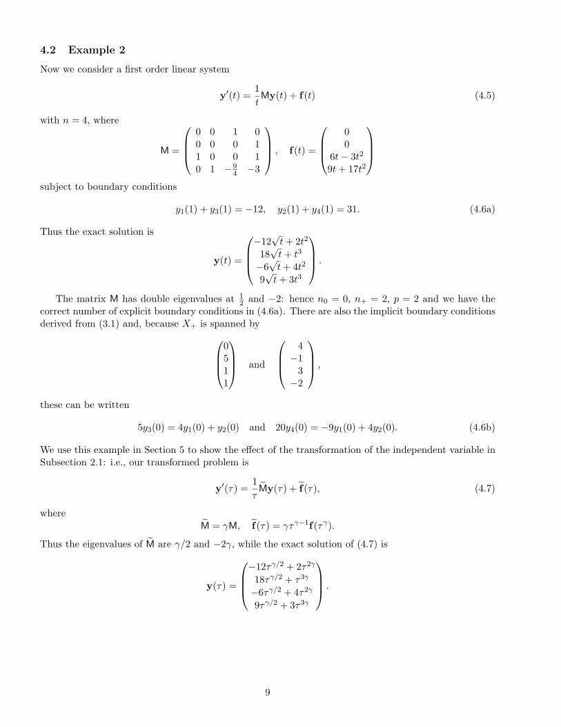
4.2 Example 2

Now we consider a first order linear system

y′(t) =1

tMy(t) + f(t) (4.5)

with n = 4, where

M =

0 0 1 00 0 0 11 0 0 10 1 −9

4 −3

, f(t) =

00

6t − 3t2

9t + 17t2

subject to boundary conditions

y1(1) + y3(1) = −12, y2(1) + y4(1) = 31. (4.6a)

Thus the exact solution is

y(t) =

−12√

t + 2t2

18√

t + t3

−6√

t + 4t2

9√

t + 3t3

.

The matrix M has double eigenvalues at 12 and −2: hence n0 = 0, n+ = 2, p = 2 and we have the

correct number of explicit boundary conditions in (4.6a). There are also the implicit boundary conditionsderived from (3.1) and, because X+ is spanned by

0511

and

4−1

3−2

,

these can be written

5y3(0) = 4y1(0) + y2(0) and 20y4(0) = −9y1(0) + 4y2(0). (4.6b)

We use this example in Section 5 to show the effect of the transformation of the independent variable inSubsection 2.1: i.e., our transformed problem is

y′(τ) =1

τMy(τ) + f(τ), (4.7)

whereM = γM, f(τ) = γτγ−1f(τγ).

Thus the eigenvalues of M are γ/2 and −2γ, while the exact solution of (4.7) is

y(τ) =

−12τγ/2 + 2τ2γ

18τγ/2 + τ3γ

−6τγ/2 + 4τ2γ

9τγ/2 + 3τ3γ

.

9

4.3 Example 3

The singular boundary value problem we discuss here originates from the Cahn-Hillard theory, whichis used in hydrodynamics to study the behavior of non-homogeneous fluids. In [13], the density profile

equation for the description of the formation of microscopic bubbles in a non-homogeneous fluid (inparticular, vapor inside liquid) is derived. After some simplifications, cf. [26], we arrive at the boundaryvalue problem

ρ′′(r) +N − 1

rρ′(r) = 4λ2(ρ(r) + 1)ρ(r)(ρ(r) − ξ), (4.8)

ρ′(0) = 0, ρ(∞) = ξ, (4.9)

where ρ is the density of the liquid surrounding the bubble. The problem (4.8), (4.9) depends on 3parameters: λ, which may be chosen as λ = 1 without restriction of generality, N which is the dimensionof the problem, which in the physically meaningful case is N = 3, and ξ, which is varied in the range [0, 1]such as to reflect different physical situations. For the numerical treatment, we transform the problemto the finite interval s ∈ [0, 1], by introducing (z1(s), z2(s))

T = (ρ(s), ρ(1/s))T and obtain,

z′′1 (s) =1 − N

sz′1(s) + 4λ2(z1(s) + 1)z1(s)(z1(s) − ξ), (4.10a)

z′′2 (s) =1

s(N − 3)z′2(s) +

4λ2

s4(z2(s) + 1)z2(s)(z2(s) − ξ), (4.10b)

subject to boundary conditions

z′1(0) = 0, z2(0) = ξ, z1(1) = z2(1), z′1(1) = −z′2(1). (4.11)

The above boundary value problem exhibits a singularity of the second kind (due to the 1/s4 term)and depends on the real parameter ξ. We solve the problem by applying the path-following strategyimplemented in bvpsuite. Due to an interior layer, the numerical treatment becomes computationallymore challenging when the value of the parameter ξ approaches 1 and it turns out that the implicit formof (4.10b),

s4z′′2 (s) = s3(N − 3)z′2(s) + 4λ2(z2(s) + 1)z2(s)(z2(s) − ξ)

considerably improves the numerical stability. For more details, see [26].

5 Numerical Results

To obtain the numerical results presented in this section, we used the Matlab code bvpsuite, which isdescribed in detail in [25]. The code is based on polynomial collocation and it is capable of solving ordinarydifferential equations directly in fully implicit form and arbitrary order (including zero, correspondingto algebraic equations). In every subinterval we make an ansatz with polynomials represented in theRunge–Kutta basis [4] of degree ≤ s for problems of first order and ≤ s + 1 for second order, wheres is the number of collocation points used in each subinterval. The collocating function is required tobe globally continuous in the first and continuously differentiable in the second case. The convergencebehavior of the collocation schemes applied to boundary value problems with a singularity of the firstkind have been studied in [21]. Stage order convergence O(hs) can be shown to hold uniformly in t.However, due to the singularity, the superconvergence orders O(h2s) for Gauss and O(h2s−2) for Lobattocannot be guaranteed, in general. The code is capable of adaptive mesh selection as described in [6],based on a posteriori estimates of the global error presented in [5]. Due to the robustness of collocation,this method was used in one of the best established standard FORTRAN codes for (regular) BVPs,COLNEW, see [2] and [3], and in bvp4c, bvp6c, the standard Matlab modules for (regular) ODEs with

10

an option for singular problems, cf. [37]. Solvable by the FORTRAN code COLNEW are explicit systemsof at most order four. The Matlab code bvp4c also solves explicit ODE systems and is based on Lobattocollocation. As with bvp4c, certain subclasses of singular boundary value problems can be also treatedby a newer ‘User-Friendly Fortran Code’, see [38]. In this paper we do not attempt to compare the abovesoftware, but rather concentrate on comparing different algorithmic variants of the collocation mentionedin the introduction.

5.1 Example 1

In the following figures and tables, the performance of different collocation schemes applied to thesecond order formulation (2.4) and the first order formulation (2.1) is compared. We give numericalresults for the parameter values µ = 3, k = 4 and α = 8; for further results and other choices of µsee [23]. All runs have been carried out in Matlab (with the floating-point relative machine accuracyof 2−52 ≈ 2.22 · 10−16) utilizing adaptive mesh selection aiming at the equidistribution of the globalerror, see [6]. The relative and absolute tolerance parameters which appear in bvpsuite were set torTOL=aTOL=Tol. For a fair comparison we proceeded as follows. The method whose name is statedin the figure’s or table’s caption was chosen to determine the final mesh on which its numerical solutionsatisfied the tolerance requirement. Two other methods shown in tables and figures were then executedon this final mesh with no error control i.e. with no mesh refinement. One of them has as manycollocation points as the leading method, which means the same amount of work, while the other onehas the same order of convergence which means the same accuracy.

In Figures 2 and 3 we give two work precision diagrams. Let the final mesh be denoted by

∆final = {t0 = 0 < t1 < . . . < tk−1 < tk . . . < tI−1 < tI = 1}

and the numerical solution at the mesh point tk by ξk. These meshes are obtained using collocation at4 Gaussian points for Figure 2 and 4 Lobatto points for Figure 3. Then work is measured by N := sI,where s is the number of collocation points used in each subinterval [tk−1, tk], and the precision is definedto be the norm of the known global error,

err = max0≤k≤I

‖ξk − z(tk)‖∞, err = max0≤k≤I

‖ξk − y(tk)‖∞,

for the problem (2.4) and (2.1), respectively. In conclusion the code bvpsuite behaves in the followingway. For singular BVPs the user can choose the default options of either equidistant or Gauss points(which are already implemented in the code) or else he can specify his own collocation points whichmust not include zero. For singular problems and Gaussian or equidistant points, the code assumes thatthe problem is well posed which means that the boundary conditions are posed in a proper way, cf.Subsections 3.1, 3.2, and [20], [40]. Lobatto points can also be implemented but they can be used onlyfor regular problems (which means that the collocation equation at t = 0 causes no problems). For theLobatto runs given in this paper we specify the necessary alternative conditions (replacing the collocationat t = 0) by something that is equivalent to (3.10). For Example 1, this condition reads y′(0) = 0. Finally,we note that the code bvpsuite can handle problems directly in higher order form or else as first ordersystems.

11

2 4 6 8 10 12 14 160

50

100

150

200

250

−log(err)N

4 Gauss4 Lobatto5 Lobatto

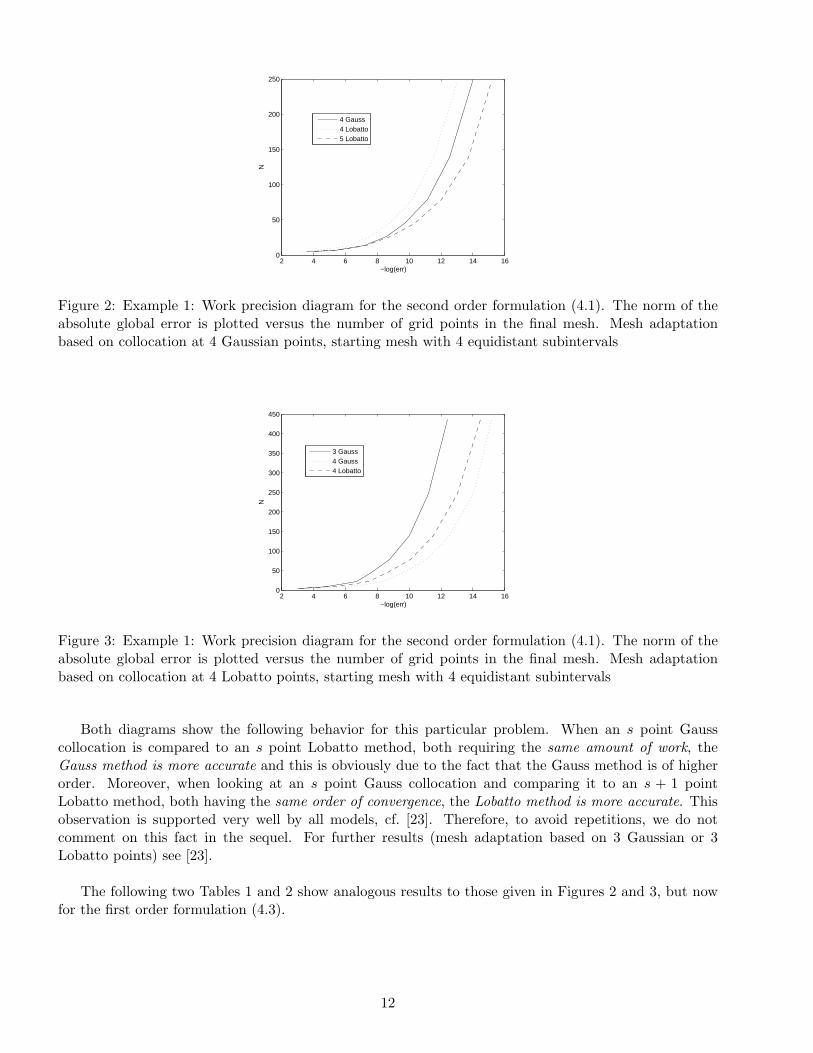
Figure 2: Example 1: Work precision diagram for the second order formulation (4.1). The norm of theabsolute global error is plotted versus the number of grid points in the final mesh. Mesh adaptationbased on collocation at 4 Gaussian points, starting mesh with 4 equidistant subintervals

2 4 6 8 10 12 14 160

50

100

150

200

250

300

350

400

450

−log(err)

N

3 Gauss4 Gauss4 Lobatto

Figure 3: Example 1: Work precision diagram for the second order formulation (4.1). The norm of theabsolute global error is plotted versus the number of grid points in the final mesh. Mesh adaptationbased on collocation at 4 Lobatto points, starting mesh with 4 equidistant subintervals

Both diagrams show the following behavior for this particular problem. When an s point Gausscollocation is compared to an s point Lobatto method, both requiring the same amount of work, theGauss method is more accurate and this is obviously due to the fact that the Gauss method is of higherorder. Moreover, when looking at an s point Gauss collocation and comparing it to an s + 1 pointLobatto method, both having the same order of convergence, the Lobatto method is more accurate. Thisobservation is supported very well by all models, cf. [23]. Therefore, to avoid repetitions, we do notcomment on this fact in the sequel. For further results (mesh adaptation based on 3 Gaussian or 3Lobatto points) see [23].

The following two Tables 1 and 2 show analogous results to those given in Figures 2 and 3, but nowfor the first order formulation (4.3).

12

4 Gauss 4 Lobatto 5 Lobatto

Tol I err err.est err err.est err err.est

10−1 5 5.4e-3 5.9e-3 1.1e-2 1.2e-2 5.4e-3 5.2e-310−2 5 5.4e-3 5.9e-3 1.1e-2 1.2e-2 5.4e-3 5.2e-310−3 7 5.4e-4 5.4e-4 1.3e-3 1.2e-3 1.8e-4 1.8e-410−4 12 3.1e-5 3.1e-5 7.2e-5 7.3e-5 3.6e-6 3.7e-610−5 21 6.4e-7 6.6e-7 1.8e-6 1.9e-6 2.0e-7 2.1e-710−6 36 2.7e-8 2.9e-8 8.5e-8 9.1e-8 6.2e-9 6.4e-910−7 61 1.9e-9 2.1e-9 6.2e-9 6.7e-9 3.9e-10 4.0e-1010−8 106 1.2e-10 1.3e-10 3.7e-10 4.0e-10 2.5e-11 2.5e-11

Table 1: Example 1, first order formulation: Mesh adaptation based on collocation at 4 Gaussian points,starting mesh with 4 equidistant subintervals. Left subcolumn – norm of the absolute global error; rightsubcolumn – norm of the error estimate

3 Gauss 4 Gauss 4 Lobatto



Table 2: Example 1, first order formulation: Mesh adaptation based on collocation at 4 Lobatto points,starting mesh with 4 equidistant subintervals. Left subcolumn – norm of the absolute global error; rightsubcolumn – norm of the error estimate

We would like to point out an important difference in running the codes in the first and second orderformulation. Let us look at the related figures and tables, Figure 2 and Table 1 or Figure 3 and Table2. It is easily seen that meshes related to the same tolerances are denser for the first order formulation,especially for stricter tolerance requirements. This is because in the second order formulation only theerrors in the solution z are controlled. When working with the first order form however, the errors ofboth components of y, y1 = z and y2 = tz′, are to be controlled. To enable a better understanding of thiseffect we carry out another test, see Tables 3 and 4. Here, we set the tolerance for the component y2 = tz′

to Tol = 1, so the error in this component is not controlled in practice. Consequently, the adaptationstrategy has to take care of y1 = z only. Still, due to the coupling of y1 and y2, the meshes stay densercompared to the second order formulation which clearly indicates that the direct treatment of the secondorder problem is more efficient, in general. For further results (mesh adaptation based on 3 Gauss or 3Lobatto points), see [23]. A final remark that we wish to make is that the quality of the error estimateis excellent throughout.

13

4 Gauss 4 Lobatto 5 Lobatto



Table 3: Example 1, first order formulation: Mesh adaptation based on collocation at 4 Gaussian points,starting mesh with 4 equidistant subintervals. Left subcolumn – norm of the absolute global error; rightsubcolumn – norm of the error estimate, tolerances only prescribed for the first component

3 Gauss 4 Gauss 4 Lobatto



Table 4: Example 1, first order formulation: Mesh adaptation based on collocation at 4 Lobatto points,starting mesh with 4 equidistant subintervals. Left subcolumn – norm of the absolute global error; rightsubcolumn – norm of the error estimate, tolerances only prescribed for the first component

5.2 Example 2

Our aim in considering this example is to experimentally investigate how the transformation t = τγ

described in Subsection 2.1 influences the convergence order of the collocation scheme and the performanceof the mesh adaptation strategy. For illustration purposes we choose γ = 10 for Example 2 and so thesolution of the transformed problem (4.7) is considerably smoother than the solution of the originalproblem (4.5). All calculations have been carried out with 4 equidistant collocation points and initialmesh with 10 equidistant subintervals. This means that the order of the method being used is 4. Thereason that we have chosen to use equidistant collocation points is to ensure that our experiments arenot complicated by superconvergence (although we do recognize the fact that superconvergence does notgenerally occur with singular problems, see [21]). By using equidistant collocation points we can be surethat any changes in the rate of convergence are caused by the eigenstructure of the problem and not byany superconvergence behaviour.

Let us consider a partition

∆i := {t0 = 0 < t1 < . . . < tk−1 < tk . . . < tI−1 < tI = t2i+1 = 1, }

of the interval of integration which consists of I = 2i+1 equidistant subintervals, and let us denote the

14

numerical solution at the mesh point k, k = 0, 1, . . . 2i+1 by ξki . Moreover, let

ξi := (ξ0i , ξ1

i , . . . , ξki , . . . , ξ2i+1

i ), yex := (y(t0),y(t1), . . . ,y(tk), . . . ,y(t2i+1)),

and‖ξi − ξi+1‖ := max

0≤k≤2i+1‖ξk

i − ξ2ki+1‖∞, ‖ξi − yex‖ := max

0≤k≤2i+1‖ξk

i − y(tk)‖∞.

In our numerical experiments the number of subintervals was doubled at each step and for twoconsecutive meshes the order of convergence conv esti was estimated. Due to the non-smoothness of theanalytical solution of (4.5), we observe a severe order reduction with the order of convergence being 0.5,see Tables 5 and 6.

i ||ξi − ξi+1|| ||ξi − yex|| conv esti1 1.8e-01 6.3e-01 0.502 1.3e-01 4.5e-01 0.503 9.3e-02 3.1e-01 0.504 6.5e-02 2.2e-01 0.505 4.6e-02 1.5e-01 —

Table 5: Example 2, first component, equidistant collocation: Left subcolumn – norm of the global errorestimate ||ξi − ξi+1||; middle subcolumn – norm of the global error in comparison to the exact solution;right subcolumn – order of convergence conv esti


Table 6: Example 2, second component, equidistant collocation: Left subcolumn – norm of the globalerror estimate ||ξi − ξi+1||; middle subcolumn – norm of the global error in comparison to the exactsolution; right subcolumn – order of convergence conv esti

The results in Tables 7 and 8 are related to the solution of the transformed problem (4.7). Due tothe extra smoothness of the solution a much better order of convergence (full stage order) is observed.


Table 7: Example 2, first component, transformed, equidistant collocation: Left subcolumn – norm ofthe global error estimate ||ξi − ξi+1||; middle subcolumn – norm of the global error in comparison to theexact solution; right subcolumn – order of convergence conv esti

15


Table 8: Example 2, second component, transformed, equidistant collocation: Left subcolumn – norm ofthe global error estimate ||ξi − ξi+1||; middle subcolumn – norm of the global error in comparison to theexact solution; right subcolumn – order of convergence conv esti

It is useful here to summarise these results. Due to the lack of smoothness in the solution of theoriginal problem which is due to small positive eigenvalues of M, we observe severe reduction of theconvergence order of the collocation scheme. After the transformation, the solution is appropriatelysmooth and the classical convergence order is observed.

We now test our mesh adaptation algorithm for the transformed problem first and for the originalone afterwards. The initial mesh contained 10 equidistant subintervals. The calculations were carriedout with 4 equidistant collocation points, and the absolute and relative error tolerances were set to 10−4.

0 0.5 1−10

−5

0

5

0 0.5 1−20

0

20

0 0.5 10

1

2

0 0.5 1−5

0

5x 10

−6

0 0.5 1−1

0

1x 10

−5

Figure 4: Example 2 (transformed version), 4 equidistant collocation points: Automatically chosen finalmesh necessary to satisfy the absolute and relative tolerance requirement 10−4. Left top – down: Firstand second solution component and the distribution of the meshpoints. Right top – down: Absoluteerror estimated for the first and second component

16

0 0.5 1−10

−5

0

5

0 0.5 1−10

0

10

20

0 0.5 10

1

2

0 0.5 1

−5

0

5

x 10−6

0 0.2 0.4 0.6 0.8

−5

0

5

x 10−6

Figure 5: Example 2 (transformed version), 4 equidistant collocation points: Automatically chosen finalmesh necessary to satisfy the absolute and relative tolerance requirement 10−4 rescaled to the originalindependent variable. Left top – down: First and second solution component and the distribution of themeshpoints. Right top – down: Absolute error estimated for the first and second component

The transformation does an extremely good job of improving the rate of convergence of our algorithm.The tolerances are satisfied on a mesh containing only 63 meshpoints. Figure 4 shows the solution andthe automatically chosen mesh for the system (4.7). When we rescale the plots in Figure 4 back to theoriginal independent variable we obtain Figure 5. The colors black and grey indicate the stretching effectof the transformation.

Finally, we apply our adaptive solution routine to the original system (4.5).

0 0.5 1−10

−5

0

0 0.5 10

10

20

0 0.5 10

1

2

0 0.1 0.2 0.3

−10

−5

0

x 10−3

0 0.2 0.4 0.6 0.8

−0.01

0

0.01

0.02

Figure 6: Example 2 (original version), 4 equidistant collocation points: Mesh containing 107 pointsafter 4 refinements, tolerances not satisfied. Left top – down: First and second solution component andthe distribution of the meshpoints. Right top – down: Absolute error estimated for the first and secondcomponent

17

Clearly the mesh adaptation algorithm does not work at all well, due to the slow convergence of themethod and the incorrect order the mesh adaptation strategy is based on. Our mesh choosing algorithmis implemented on the assumption that the order of convergence is s = 4 but in this example the order ofconvergence is in fact 0.5. The very poor performance of the mesh choosing algorithm can be seen fromFigure 6 and we stopped the calculations with a mesh containing around 700 points without reaching therequired accuracy.

5.3 Example 3

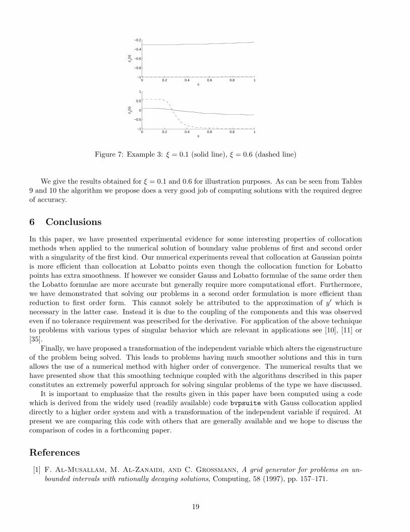
In this section, we only report on the solution for two different values of the parameter ξ. The numericalsolution is shown in Figure 7.

3 Gauss 4 Gauss 5 Gauss

Tol I err.est I err.est I err.est

10−1 4 3.0e-3 4 4.4e-4 4 8.5e-510−2 4 3.0e-3 4 4.4e-4 4 8.5e-510−3 4 3.0e-3 4 4.4e-4 4 8.5e-510−4 11 3.4e-5 8 1.2e-6 4 8.5e-510−5 20 3.6e-6 8 1.2e-6 8 3.5e-810−6 34 2.6e-7 8 1.2e-6 8 3.5e-810−7 61 1.5e-8 19 6.5e-8 8 3.5e-810−8 108 1.1e-9 31 2.6e-9 20 9.3e-910−9 192 7.6e-11 48 4.4e-10 29 1.0e-910−10 340 4.6e-12 76 4.3e-11 43 3.8e-11

Table 9: Example 3, ξ = 0.1: Numerical solution obtained with mesh adaptation based on collocation at3, 4, and 5 Gaussian points, starting mesh with 4 equidistant subintervals

3 Gauss 4 Gauss 5 Gauss

Tol I err.est I err.est I err.est

10−1 8 5.6e-2 8 1.7e-2 8 1.6e-310−2 12 1.2e-2 8 1.7e-2 8 1.6e-310−3 21 5.0e-4 13 5.0e-4 8 1.6e-310−4 37 5.4e-6 21 1.5e-5 11 2.0e-410−5 66 3.2e-7 32 4.1e-7 16 2.4e-610−6 117 1.9e-8 51 3.3e-8 23 1.4e-710−7 207 1.1e-9 81 2.1e-9 34 8.1e-910−8 368 5.8e-11 128 1.4e-10 50 5.7e-1010−9 654 3.3e-12 202 9.6e-12 73 4.8e-1110−10 1163 1.9e-13 320 7.2e-13 107 3.5e-12

Table 10: Example 3, ξ = 0.6: Numerical solution obtained with mesh adaptation based on collocationat 3, 4, and 5 Gaussian points, starting mesh with 8 equidistant subintervals

18

0 0.2 0.4 0.6 0.8 1−1

−0.8

−0.6

−0.4

−0.2

s

z 1(s)

0 0.2 0.4 0.6 0.8 1−1

−0.5

0

0.5

1

s

z 2(s)

Figure 7: Example 3: ξ = 0.1 (solid line), ξ = 0.6 (dashed line)

We give the results obtained for ξ = 0.1 and 0.6 for illustration purposes. As can be seen from Tables9 and 10 the algorithm we propose does a very good job of computing solutions with the required degreeof accuracy.

6 Conclusions

In this paper, we have presented experimental evidence for some interesting properties of collocationmethods when applied to the numerical solution of boundary value problems of first and second orderwith a singularity of the first kind. Our numerical experiments reveal that collocation at Gaussian pointsis more efficient than collocation at Lobatto points even though the collocation function for Lobattopoints has extra smoothness. If however we consider Gauss and Lobatto formulae of the same order thenthe Lobatto formulae are more accurate but generally require more computational effort. Furthermore,we have demonstrated that solving our problems in a second order formulation is more efficient thanreduction to first order form. This cannot solely be attributed to the approximation of y′ which isnecessary in the latter case. Instead it is due to the coupling of the components and this was observedeven if no tolerance requirement was prescribed for the derivative. For application of the above techniqueto problems with various types of singular behavior which are relevant in applications see [10], [11] or[35].

Finally, we have proposed a transformation of the independent variable which alters the eigenstructureof the problem being solved. This leads to problems having much smoother solutions and this in turnallows the use of a numerical method with higher order of convergence. The numerical results that wehave presented show that this smoothing technique coupled with the algorithms described in this paperconstitutes an extremely powerful approach for solving singular problems of the type we have discussed.

It is important to emphasize that the results given in this paper have been computed using a codewhich is derived from the widely used (readily available) code bvpsuite with Gauss collocation applieddirectly to a higher order system and with a transformation of the independent variable if required. Atpresent we are comparing this code with others that are generally available and we hope to discuss thecomparison of codes in a forthcoming paper.

References

[1] F. Al-Musallam, M. Al-Zanaidi, and C. Grossmann, A grid generator for problems on un-

bounded intervals with rationally decaying solutions, Computing, 58 (1997), pp. 157–171.

19

[2] U. Ascher, J. Christiansen, and R. Russell, A collocation solver for mixed order systems of

boundary values problems, Math. Comp., 33 (1978), pp. 659–679.

[3] , Collocation software for boundary value ODEs, ACM Transactions on Mathematical Software,7 (1981), pp. 209–222.

[4] U. Ascher, R. Mattheij, and R. Russell, Numerical Solution of Boundary Value Problems for

Ordinary Differential Equations, Prentice-Hall, Englewood Cliffs, NJ, 1988.

[5] W. Auzinger, O. Koch, D. Praetorius, and E. Weinmuller, New a posteriori error estimates

for singular boundary value problems, Numer. Algorithms, 40 (2005), pp. 79–100.

[6] W. Auzinger, O. Koch, and E. Weinmuller, Efficient mesh selection for collocation methods

applied to singular BVPs, J. Comput. Appl. Math., 180 (2005), pp. 213–227.

[7] C. Budd, J. Chen, and V. A. Galaktionov, Focusing blow-up for quasilinear parabolic equations,Proc. R. Soc. Edinb., 128A (1998), pp. 965–992.

[8] C. Budd, V. A. Galaktionov, and J. F. Williams, Self-similar blow-up in higher-order semi-

linear parabolic equations, Preprint 02/10, Dept. Math. Sci., Univ. of Bath, 2002.

[9] C. J. Budd, S. Chen, and R. D. Russell, New self-similar solutions of the nonlinear Schrodinger

equation with moving mesh computations, J. Comput. Phys., 152 (1999), pp. 756–789.

[10] C. J. Budd, O. Koch, and E. Weinmuller, Computation of self-similar solution profiles for the

nonlinear Schrodinger equation, 77 (2006), pp. 335–346.

[11] , From nonlinear PDEs to singular ODEs, Appl. Numer. Math., 56 (2006), pp. 413–422.

[12] J. Cash and H. Silva, On the numerical solution of a class of singular two-point boundary value

problems, J. Comput. Appl. Math., 45 (1993), pp. 91–102.

[13] F. Dell’Isola, H. Gouin, and G. Rotoli, Nucleation of spherical shell-like interfaces by second

gradient theory: Numerical simulations, Eur. J. Mech. B/Fluids, 15 (1996), pp. 545–568.

[14] M. Duhoux, Nonlinear singular Sturm-Liouville problems, Nonlinear Anal., 38A (1999), pp. 897–918.

[15] M. El-Gebeily and I. Abu-Zaid, On a finite difference method for singular two-point boundary

value problems, IMA J. Numer. Anal., 18 (1998), pp. 179–190.

[16] R. Fazio, A novel approach to the numerical solution of boundary value problems on infinite inter-

vals, SIAM J. Numer. Anal., 33 (1996), pp. 1473–1483.

[17] A. Fink, J. Gatica, G. Hernandez, and P. Waltman, Approxomation of solutions of singular

second-order boundary value problems, SIAM J. Math. Anal., 22 (1991), pp. 440–462.

[18] I. Gohberg, P. Lancaster, and L. Rodman, Matrix Polynomials, Academic Press, NewYork,1982.

[19] G. H. Golub and C. F. Van Loan, Matrix Computations, The John Hopkins University Press,Baltimore, 2nd ed., 1989.

[20] F. d. Hoog and R. Weiss, Difference methods for boundary value problems with a singularity of

the first kind, SIAM J. Numer. Anal., 13 (1976), pp. 775–813.

20

[21] , Collocation methods for singular boundary value problems, SIAM J. Numer. Anal., 15 (1978),pp. 198–217.

[22] S. Iyengar and P. Jain, Spline finite difference methods for singular two-point boundary value

problems, Numer. Math., 50 (1987), pp. 363–376.

[23] G. Kitzhofer, Numerical Treatment of Implicit Singular BVPs, Ph.D. Thesis, Inst. for Anal. andSci. Comput., Vienna Univ. of Technology, Austria. In preparation.

[24] G. Kitzhofer, O. Koch, P. Lima, and E. Weinmuller, Efficient numerical solution of the

density profile equation in hydrodynamics, J. Sci. Comput., 32 (2007), pp. 414–424.

[25] G. Kitzhofer, O. Koch, and E. Weinmuller, An Efficient General Purpose Code for Implicit

ODEs of Arbitrary Order. In preparation.

[26] , Collocation methods for the computation of bubble-type solutions of a singular bound-

ary value problem in hydrodynamics, Techn. Rep. ANUM Preprint Nr. 14/04, Inst. forAnal. and Sci. Comput., Vienna Univ. of Technology, Austria, 2004. Available athttp://www.math.tuwien.ac.at/~inst115/preprints.htm.

[27] O. Koch and E. Weinmuller, Analytical and numerical treatment of a singular initial value

problem in avalanche modeling, Appl. Math. Comput., 148 (2004), pp. 561–570.

[28] N. Konyukhova, P. Lima, and M. Carpentier, Asymptotic and numerical approximation of

nonlinear singular bounadry value problem, Tendencias em Matematica Aplicada e Computacional,(2002).

[29] P. Lima, N. Chemetov, N. Konyukhova, and A. Sukov, Analytical-numerical approach to a

singular boundary value problem. Proceedings of CILAMCE XXIV, Ouro Preto, Brasil.

[30] X. Liu, A note on the Sturmian Theorem for singular boundary value problems, J. Math. Anal. Appl.,237 (1999), pp. 393–403.

[31] R. Marz and E. Weinmuller, Solvability of boundary value problems for systems of singular

differential-algebraic equations, SIAM J. Math. Anal., 24 (1993), pp. 200–215.

[32] D. M. McClung and A. I. Mears, Dry-flowing avalanche run-up and run-out, J. Glaciol., 41(1995), pp. 359–369.

[33] G. Moore, Computation and parametrization of periodic and connecting orbits, IMA J. Nu-mer. Anal., 15 (1995), pp. 245–263.

[34] , Geometric methods for computing invariant manifolds, Appl. Numer. Math., 17 (1995),pp. 319–331.

[35] I. Rachunkova, O. Koch, G. Pulverer, and E. Weinmuller, On a singular boundary value

problem arising in the theory of shallow membrane caps, 332 (2007), pp. 523–541. To appear inMath. Anal. and Appl.

[36] P. Rentrop, Eine Taylorreihenmethode zur numerischen Losung von Zwei-Punkt Randwertprob-

lemen mit Anwendung auf singulare Probleme der nichtlinearen Schalentheorie. TUM-MATH-7733.Technische Universitat Munchen 1977.

[37] L. Shampine, J. Kierzenka, and M. Reichelt, Solving Boundary Value Prob-

lems for Ordinary Differential Equations in Matlab with bvp4c, 2000. Available atftp://ftp.mathworks.com/pub/doc/papers/bvp/.

21

[38] L. Shampine, P. Muir, and H. Xu, A User-Friendly Fortran BVP Solver, Available athttp://cs.smu.ca/~muir/BVP SOLVER Files/ShampineMuirXu2006.pdf, (2006).

[39] J. Tuomela, A geometric analysis of singular ODE related to the study of quasilinear PDE, Electron.J. Differential Equations, 62 (2000), pp. 1–6.

[40] E. Weinmuller, On the boundary value problems for systems of ordinary second order differential

equations with a singularity of the first kind, SIAM J. Math. Anal., 15 (1984), pp. 287–307.

[41] , Testing of error estimation procedures for singular boundary value problems, CMS Conf. Proc.,8 (1987), pp. 135–152.

Jeff R. Cashhttp://www.ma.ic.ac.uk/∼jcash/, [email protected] Moorehttp://www.ma.ic.ac.uk/∼gmoore/, [email protected]

Imperial College LondonSouth Kensington CampusDepartment of MathematicsLondon, SW7 2AZ, United Kingdom

Georg Kitzhoferhttp://www.math.tuwien.ac.at/georg/, [email protected] Kochhttp://www.othmar-koch.org/, [email protected] Weinmullerhttp://www.math.tuwien.ac.at/∼ewa/, [email protected]

Vienna University of TechnologyInstitute for Analysis and Scientific ComputingWiedner Hauptstrasse 8-10A-1040 Wien, Austria

22

Numerical Solutions of singular Two Point BVPsNumerical Solution of Singular Two Point BVPs J.Cash,...

Documents

Transcript of Numerical Solutions of singular Two Point BVPsNumerical Solution of Singular Two Point BVPs J.Cash,...