Numerical Solution of the Nonlinear Poisson-Boltzmann...

Numerical Solution of the Nonlinear Poisson-BoltzmannEquation: Developing More Robust and Efficient Methods

Michael J. Holst

Department of Applied Mathematics and CRPCCalifornia Institute of Technology 217-50Pasadena, CA USA 91125

Faisal Saied

Department of Computer Science1304 West Springfield AvenueUrbana, IL USA 61801

We present a robust and efficient numerical method for solution of the nonlinear Poisson-Boltzmann equation arisingin molecular biophysics. The equation is discretized with the box method, and solution of the discrete equations isaccomplished with a global inexact-Newton method, combined with linear multilevel techniques we have described in apaper appearing previously in this journal. A detailed analysis of the resulting method is presented, with comparisonsto other methods that have been proposed in the literature, including the classical nonlinear multigrid method, thenonlinear conjugate gradient method, and nonlinear relaxation methods such as successive over-relaxation. Boththeoretical and numerical evidence suggests that this method will converge in the case of molecules for which manyof the existing methods will not. In addition, for problems which the other methods are able to solve, numericalexperiments show that the new method is substantially more efficient, and the superiority of this method grows withthe problem size. The method is easy to implement once a linear multilevel solver is available, and can also easily beused in conjunction with linear methods other than multigrid.

INTRODUCTION

In this paper, we consider numerical solution of the non-linear Poisson-Boltzmann equation (PBE), the funda-mental equation arising in the Debye-Huckel theory [1]of continuum molecular eletrostatics. In the case of a1 : 1 electrolyte, this equation can be written as

−∇ · (ε(r)∇u(r)) + κ2(r) sinh(u(r))

=4πe2

c

kBT

Nm∑

i=1

ziδ(r − ri), u(∞) = 0, (1)

a three-dimensional second order nonlinear partial dif-ferential equation governing the dimensionless electro-static potential u(r) = ecΦ(r)/k−1

B T−1, where Φ(r) isthe electrostatic potential at a field position r. The im-portance of this equation for modeling biomolecules iswell-established; more detailed discussions of the use ofthe Poisson-Boltzmann equation may be found in thesurvey articles of Briggs and McCammon [2] and Sharpand Honig [3].

In the equation above, the coefficient ε(r) jumps bymore than an order of magnitude across the interface be-tween the molecule and surrounding solvent. The modi-fied Debye-Huckel parameter κ, proportional to the ionicstrength of the solution, is discontinuous at the interfacebetween the solvent region and an ion exclusion layersurrounding the molecular surface. The molecule itselfis represented by Nm point charges qi = ziec at posi-tions ri, yielding the delta functions in (1), and the con-stants ec, kB , and T represent the charge of an electron,Boltzmann’s constant, and the absolute temperature.Equation (1) is referred to as the nonlinear Poisson-Boltzmann equation, and it is often approximated by thelinearized Poisson-Boltzmann equation, obtained by tak-ing sinh(u(r)) ≈ u(r) when u(r) << 1.

In the nonlinear case, equation (1) presents severe nu-merical difficulties due to the rapid exponential nonlin-

earities, discontinuous coefficients, delta functions, andinfinite domain. In this article, we present a survey ofthe numerical methods currently employed in the bio-physics and biochemistry communities for the linearizedand nonlinear Poisson-Boltzmann equations. We thenpropose an alternative numerical method, which is acombination of global inexact-Newton methods and mul-tilevel methods. A detailed analysis of this methodis presented, with comparisons to other methods thathave been proposed in the literature, including the clas-sical nonlinear multigrid method, the nonlinear conju-gate gradient method, and nonlinear relaxation meth-ods such as successive over-relaxation. Both theoreticaland numerical evidence shows that the global inexact-Newton-multilevel method is superior to all other meth-ods currently in use. In particular, this method is morerobust (it converges in cases where the other methodsfail) and substantially more efficient (the advantage ofthis method grows with the problem size). The methodis easy to implement once a linear multilevel solver isavailable, and can also easily be used in conjunction withlinear methods other than multigrid (the robustness ismaintained, although the efficiency may be less).

Outline

We begin by discussing the form of the algebraic equa-tions which are produced by standard discretizationmethods applied to equation (1). We then briefly re-view the methods that have been proposed and usedfor the linearized Poisson-Boltzmann equation, includ-ing the linear multilevel method we have presented ina previous paper. We then discuss in a little more de-tail the methods recently proposed in the literature forthe nonlinear Poisson-Boltzmann equation, and presentinexact-Newton methods as alternatives. We formulatean algorithm based on the combination of global inexact-Newton methods and our linear multilevel method, and

2 HOLST

we state and prove two simple conditions which guaran-tee that the resulting inexact-Newton-multilevel methodis globally convergent. Some test problems are then for-mulated, including some more difficult problems involv-ing superoxide dismutase (SOD) and tRNA. Numericalexperiments are then presented, showing that in fact theNewton-multilevel approach is both more robust and or-ders of magnitude more efficient than existing methods.

Due to the length of the paper, we also give a moredetailed outline of the material below.

DISCRETIZING THE PBE 2

The box-method approach . . . . . . . . . . . . 2Non-uniform Cartesian meshes . . . . . . . . . 3The algebraic equations . . . . . . . . . . . . . 4

LINEARIZED PBE METHODS 4

Classical linear methods . . . . . . . . . . . . . 5Linear conjugate gradient methods . . . . . . . 6Linear multilevel methods . . . . . . . . . . . . 7

NONLINEAR PBE METHODS 8

Nonlinear relaxation methods . . . . . . . . . . 8Nonlinear conjugate gradient methods . . . . . 9Nonlinear multilevel methods . . . . . . . . . . 10

INEXACT-NEWTON METHODS 12

Inexactness and superlinear convergence . . . . 13Inexactness and global convergence . . . . . . . 14Inexact-Newton-MG for the PBE . . . . . . . . 15

SOME TEST PROBLEMS 17

The nonlinear PBE . . . . . . . . . . . . . . . . 17Brookhaven data and existing software . . . . . 18Polynomial nonlinear forms of the PBE . . . . 18A nonlinear jump discontinuity problem . . . . 19

NUMERICAL COMPARISONS 19

Results for acetamide . . . . . . . . . . . . . . 20Results for crambin . . . . . . . . . . . . . . . . 20Results for tRNA . . . . . . . . . . . . . . . . . 20Results for SOD . . . . . . . . . . . . . . . . . 20Jump discontinuity problem results . . . . . . . 20Storage requirements . . . . . . . . . . . . . . . 23

CONCLUSIONS 23

REFERENCES 25

DISCRETIZING THE PBE

The infinite domain of equation (1) is often truncated toa finite domain Ω ⊂ R

3 with boundary Γ, and boundary

conditions on Γ are provided by a known analytical so-lution; detailed discussions appear in Tanford [4] and inreferences [5, 6]. The equation then becomes:

−∇ · (ε∇u) + κ sinh(u) = f in Ω ⊂ R3, (2)

u = g on Γ,

where the source term in equation (1) has been denotedas the generic function f . The functions ε and κ may beonly piecewise continuous functions on Ω, although weassume that the coefficient discontinuities are regular,and can be identified during the discretization process.In particular, to discretize (2) accurately, the domainΩ must be divided into discrete elements such that thediscontinuities always lie along element boundaries, andnever within an element. While this is not completelypossible, it is important to achieve this as much as possi-ble due to discrete approximation theory considerations(cf. the texts by Varga [7] and Strang and Fix [8]).

We begin by partitioning the domain Ω into the finiteelements or volumes τ j , such that:

• Ω ≡⋃M

j=1 τ j , where the elements τ j are for exam-ple hexahedra or tetrahedra.

• The discontinuities in the coefficients ε, κ, f aretaken to lie along the boundaries of τ j .

• The union of the (4 or 8) corners of the τ j formthe nodes xi in the resulting mesh of nodes.

• The set τ j;i ≡ τ j : xi ∈ τ j consists of allelements τ j;i having xi as a corner.

• Define τ (i) ≡⋃

j τ j;i ≡ ⋃

j τ j : xi ∈ τ j to be the

“box” around xi formed by union of the τ j;i.

• We require continuity of u and a∇u · n across theregions having different values of a.

The box (integral, finite volume) method has beenone of the standard approaches for discretizing two- andthree-dimensional interface problems occurring in reac-tor physics and reservoir simulation [7, 9]; similar meth-ods are used in computational fluid dynamics. The mo-tivation for these methods has been the attempt to en-force conservation of certain physical quantities in thediscretization process.

The box-method approach

We begin by integrating (2) over an arbitrary τ (i). Theresulting equation is:

∫

τ (i)

(−∇ · (ε∇u) + κ sinh(u) dx − f) dx = 0.

NUMERICAL SOLUTION OF THE NONLINEAR POISSON-BOLTZMANN EQUATION 3

Recalling the definition of τ (i) as the union over j of theτ j;i, and employing the divergence theorem for the firstterm in the equation above, yields:

−∑

j

∫

∂τj;i

(ε∇u)·n ds+∑

j

∫

τj;i

(κ sinh(u) − f) dx = 0,

where ∂τ j;i is the boundary of τ j;i and n is the unitnormal. Note that all interior surface integrals in thefirst term vanish, since ε∇u·n must be continuous acrossthe interfaces. We are left with:

−

∫

∂τ (i)

(ε∇u) · n ds +∑

j

∫

τj;i

(κ sinh(u) − f) dx = 0,

where ∂τ (i) denotes the boundary of τ (i).Since this last relationship holds exactly in each τ (i),

we can use this last equation to develop an approxima-tion at the nodes xi = (xi, yi, zi) ∈ R

3 at the “centers” ofthe τ (i) by employing quadrature rules and difference for-mulas. In particular, the volume integrals in the secondtwo terms can be approximated with quadrature rules.Similarly, the surface integrals required to evaluate thefirst term can be approximated with quadrature rules,where ∇u is replaced with an approximation. Errorestimates can be obtained from difference and quadra-ture formulas [7], or more generally by analyzing thebox-method as a special Petrov-Galerkin finite elementmethod [10, 11].

Non-uniform Cartesian meshes

The methods we develop in this paper for solving non-linear algebraic equations can be applied quite gener-ally to the equations arising from box or finite elementmethod discretizations of nonlinear elliptic equations onvery general non-Cartesian meshes. However, a few ofthe algebraic multilevel techniques we employ (discussedin more detail later in the paper and in [5, 6]) requirelogically Cartesian meshes. Note that logically Cartesianrequires only that each mesh point have a nearest neigh-bor structure as for uniform Cartesian meshes, althoughthe mesh lines need not be uniformly spaced, and themesh axes need not be orthogonal, or even consist ofstraight lines at all. A logically Cartesian mesh is thenclearly much more general than a non-uniform Carte-sian mesh, which imposes the additional restriction thatthe axes consist of orthogonal straight lines. An exampleof a three-dimensional non-uniform Cartesian mesh, em-ploying Chebyshev spacings around a centrally refinedregion, is shown in Figure 1.

Our implementations of the methods described inthis paper, with which we will present numerical ex-periments in the sections to follow, are designed to al-low a non-uniform Cartesian mesh to be employed, suchas the mesh in Figure 1. The implementations treat

Figure 1: A 3D non-uniform Cartesian mesh.

all meshes as general non-uniform Cartesian meshes; nouniform mesh simplifications are employed. When pos-sible, we will employ an adapted non-uniform Cartesianmesh, in order to discretize the given elliptic equationas accurately as possible near coefficient interfaces (forexample, the nonlinear jump discontinuity test problemappearing later in the paper). Some of the numericalexamples we consider, employing actual molecular data,require discretization on a uniform Cartesian mesh, sincethe sources of data currently available to us produce in-formation only on uniform meshes (this is discussed inmore detail later in the paper).

In this section we will therefore describe the boxmethod in the case of a non-uniform Cartesian mesh,so that the τ j appearing above are hexahedral elements,whose six sides are parallel to the coordinate axes. Byrestricting our discussion to elements which are non-uniform Cartesian, the spatial mesh may be character-ized by the nodal points

x = (x, y, z) such that

x ∈ x0, x1, . . . , xI+1y ∈ y0, y1, . . . , yJ+1z ∈ z0, z1, . . . , zK+1

.

Any such mesh point we denote as xijk = (xi, yj , zk),and we define the mesh spacings as

hi = xi+1 − xi, hj = yj+1 − yj , hk = zk+1 − zk,

which are not required to be equal or uniform.To each mesh point xijk = (xi, yj , zk), we associate

the closed three-dimensional hexahedral region τ (ijk)

“centered” at xijk , defined by

x ∈

[

xi −hi−1

2, xi +

hi

2

]

, y ∈

[

yj −hj−1

2, yj +

hj

2

]

,

4 HOLST

z ∈

[

yk −hk−1

2, zk +

hk

2

]

.

Integrating (2) over τ (ijk) for each mesh-point xijk andemploying the divergence theorem as above yields as be-fore:

−

∫

∂τ (ijk)

(ε∇u) · n ds +

∫

τ (ijk)

(κ sinh(u) − f) dx = 0.

The volume integrals are approximated with quadrature:

∫

τ (ijk)

p dx ≈ meas(τ (ijk))pijk ,

where pijk = p(xijk), and where the volume of τ (ijk) is

meas(τ (ijk)) =

[

(hi−1 + hi)(hj−1 + hj)(hk−1 + hk)

8

]

.

Since ε is a scalar, the surface integral reduces to:

∫

∂τ (ijk)

ε(ux + uy + uz) · n ds.

This integral reduces further to six two-dimensionalplane integrals on the six faces of the τ (ijk), and areapproximated with the analogous two-dimensional rule,after approximating the partial derivatives with cen-tered differences. Introducing the notation pi−1/2,j,k =p(xi−hi−1/2, yj , zk), and pi+1/2,j,k = p(xi+hi/2, yj , zk),the resulting discrete equations can be written as:

εi−1/2,j,k

(

uijk − ui−1,j,k

hi−1

)

(hj−1 + hj)(hk−1 + hk)

4

+εi+1/2,j,k

(

uijk − ui+1,j,k

hi

)

(hj−1 + hj)(hk−1 + hk)

4

+εi,j−1/2,k

(

uijk − ui,j−1,k

hj−1

)

(hi−1 + hi)(hk−1 + hk)

4

+εi,j+1/2,k

(

uijk − ui,j+1,k

hj

)

(hi−1 + hi)(hk−1 + hk)

4

+εi,j,k−1/2

(

uijk − ui,j,k−1

hk−1

)

(hi−1 + hi)(hj−1 + hj)

4

+εi,j,k+1/2

(

uijk − ui,j,k+1

hk

)

(hi−1 + hi)(hj−1 + hj)

4

+meas(τ (ijk)) (κijk sinh(uijk) − fijk) = 0.

We have one such nonlinear algebraic equation for eachuijk approximating u(xijk) at the nodes:

xijk ; i = 0, . . . , I+1; j = 0, . . . , J+1; k = 0, . . . , K+1.

This set of equations represents the nonlinear algebraicsystem which we consider for the remainder of the paper.

The algebraic equations

After using the Dirichlet boundary data from (2), onlyequations for the interior nodes remain:

xijk ; i = 1, . . . , I ; j = 1, . . . , J ; k = 1, . . . , K.

We denote the total number of unknowns in the systemof equations as n = I · J · K, and it is convenient toconsider a vector-oriented ordering of the unknowns. Forthe non-uniform Cartesian mesh we have described, thenatural ordering is defined as:

xp = xijk , p = (k − 1) · I · J + (j − 1) · I + i,

where

i = 1, . . . , I ; j = 1, . . . , J ; k = 1, . . . , K,

which defines a one-to-one mapping between xp and xijk ,and defines xp for p = 1, . . . , n. Employing the naturalordering of the meshpoints to order the unknowns ui inthe vector u yields a single nonlinear algebraic system ofequations of the form:

Au + N(u) − f = 0, (3)

where the vector f consists of components meas(τ (i))fi

for each of the mesh points xi, and the function N(u) isa nonlinearity with “diagonal form”, in that N(u) =(N1(u), . . . , Nn(u))T , with Ni(u) = Ni(ui). Here,Ni(ui) = meas(τ (i))κ(xi) sinh(ui). In the linear case,Ni(ui) = meas(τ (i))κ(xi)ui.

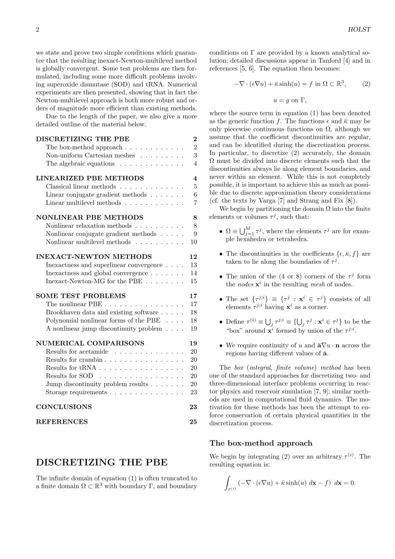
The natural ordering of the unknowns ui gives riseto a matrix A representing the linear part of (3) which isseven-banded and block-tridiagonal. This banded struc-ture in the case of non-uniform Cartesian meshes allowsfor very efficient implementations of iterative methodsfor numerical solution of the discrete linear and non-linear equations; the seven-banded form is depicted inFigure 2 for a 3 × 3 × 3 non-uniform Cartesian mesh.

It is not difficult to show [5, 6] that the matrix Ain (3) arising from box method discretization on a non-uniform Cartesian mesh is symmetric positive definite(SPD). This symmetry property holds for both box andfinite element method discretizations on very generalmeshes, and is a consequence of the fact that the originaldifferential operator is formally self-adjoint. Note thatsimple finite differences do not naturally produce sym-metric matrices from self-adjoint differential operatorsexcept for fully uniform Cartesian meshes, unless veryspecial care is taken.

Much more difficult questions, which we will not con-sider further here, are the well-posedness of the full non-linear system (3), as well as the original continuous prob-lem (2). It can be shown that both (3) and (2) haveunique solutions depending continuously on the problemdata. These and other technical questions are addressedquite fully in references [5, 6].


Figure 2: Banded matrix produced by the box-method.

LINEARIZED PBE METHODS

If the nonlinear term in equation (3) is zero, Ni(ui) ≡ 0,or if it is linear, Ni(ui) = h2κ(xi)ui, in which case theterm can be added to the diagonal of the matrix A in (3),then we are faced with linear algebraic equations:

Au = f, (4)

where the matrix A is symmetric positive definite (SPD).The matrix A is a linear operator mapping R

n into Rn,

the space Rn being a linear space equipped with an inner-

product (·, ·) inducing a norm ‖ · ‖ defined as follows:

(u, v) =

n∑

i=1

uivi, ‖u‖ = (u, u)1/2, ∀u, v ∈ Rn.

Since the matrix A is SPD, it defines a second inner-product and norm:

(u, v)A = (Au, v), ‖u‖A = (u, u)1/2A , ∀u, v ∈ R

n.

While our purpose here is not to discuss the mathemati-cal structure of R

n, the importance of either norm whichwe may associate with R

n (and hence the inner-productwhich induces the particular norm) is that the norm de-fines a metric or distance function on the space R

n, whichallows us to measure the distance between points in R

n.Equipped with only the inner-product and norm on R

n,one can establish simple conditions for linear and non-linear iterative methods to guarantee certain desirableconvergence properties.

Classical linear methods

Linear iteration methods for solving the equation (4) forthe unknown u can be thought of as having the form:

Algorithm 1 (Basic Linear Method for Au = f)

ui+1 = ui + B(f − Aui) = (I − BA)ui + Bf,

where B is an SPD matrix approximating A−1 in somesense, and where the method begins with some initial“guess” at the true solution u, namely u0. Subtractingthe above equation from the following identity for thetrue solution u:

u = u − BAu + Bf,

yields an equation for the error ei = u − ui at eachiteration of the method:

ei+1 = (I − BA)ei = · · · = (I − BA)i+1e0. (5)

The convergence of Algorithm 1, which refers to thequestion of whether ui → u (or equivalently ei → 0)as i → ∞, is determined completely by the spectral ra-dius (the eigenvalue of largest magnitude) of the errorpropagation operator:

E = I − BA,

which we denote as ρ(E).

Theorem 1 The condition ρ(E) < 1 is necessary andsufficient for convergence of Algorithm 1.

Proof. See for example Theorem 7.1.1 in Ortega [12].

If λ is an eigenvalue of E, then since |λ|‖u‖ = ‖λu‖ =‖Eu‖ ≤ ‖E‖ ‖u‖ for any norm ‖·‖, it follows that ρ(E) ≤‖E‖ for all norms ‖ · ‖ (equality holds if and only if E issymmetric with respect the inner-product defining ‖ · ‖).Therefore, ‖E‖ < 1 and ‖E‖A < 1 are both sufficientconditions for convergence of Algorithm 1. In fact, itis the norm of the error propagation operator which willbound the reduction of the error at each iteration, whichfollows from (5):

‖ei+1‖A ≤ ‖E‖A‖ei‖A ≤ ‖E‖i+1

A ‖e0‖A. (6)

The spectral radius ρ(E) of the error propagator E iscalled the convergence factor for Algorithm 1, whereasthe norm of the error propagator ‖E‖ is referred to asthe contraction number (with respect to the particularchoice of norm ‖ · ‖).

We mention now some classical linear iterations fordiscrete elliptic equations Au = f , where A is an SPDmatrix. Since A is SPD, we may write A = D−L−LT ,and where D is a diagonal matrix and L a strictly lower-triangular matrix. Some of the classical variations ofAlgorithm 1 take as B ≈ A−1 the following:

6 HOLST

(1) Richardson: B = λ−1max(A)

(2) Jacobi: B = D−1

(3) Gauss-Seidel: B = (D − L)−1

(4) SOR: B = ω(D − ωL)−1

Consider the case of the Poisson equation with zeroDirichlet boundary conditions discretized with the box-method on a uniform mesh with m mesh-points in eachmesh direction (n = m3) and mesh spacing h = 1/(m +1). This is equation (2) with ε ≡ 1 and κ ≡ 0. In thiscase, the eigenvalues of both A and the error propagationmatrix E can be determined analytically, allowing foran analysis of the convergence rates of the Richardson,Jacobi, Gauss-Seidel, and SOR iterations:

(1) Richardson: ρ(E) = 1 − O(h2)(2) Jacobi: ρ(E) = 1 − O(h2)(3) Gauss-Seidel: ρ(E) = 1 − O(h2)(4) SOR: ρ(E) = 1 − O(h)

The same dependence on h is exhibited for one- andtwo-dimensional problems. Therein lies the fundamentalproblem with all classical relaxation methods: as h → 0,then for the classical methods ρ(E) → 1, so that themethods converge more and more slowly as the problemsize is increased. This same behavior is also demon-strated for discretized forms of more general equationson more general meshes, such as those considered in thispaper.

In the paper of Nicholls and Honig [13], an adaptiveSOR procedure is developed for the linearized Poisson-Boltzmann equation, employing a power method to es-timate the largest eigenvalue of the Jacobi iteration ma-trix, which enables estimation of the optimal relaxationparameter for SOR using Young’s formula (page 110 inVarga [7]). The eigenvalue estimation technique em-ployed is similar to the power method approach dis-cussed on page 284 in Varga [7]. In the implemen-tation of the method in the computer program DEL-PHI, several additional techniques are employed to in-crease the efficiency of the method. In particular, ared/black ordering is employed allowing for vectoriza-tion, and array-oriented data structures (as opposed tothree-dimensional grid data structures) are employed tomaximize vector lengths. The implementation is alsospecialized to the linearized Poisson-Boltzmann equa-tion, with constants hard-coded into the loops ratherthan loaded as vectors to reduce vector loads.

In several recent papers [5, 6, 14], we considered anSOR method provided with the optimal relaxation pa-rameter, implemented with a red/black ordering and ar-ray oriented data structures, yielding maximal vectorlengths and very high performance on both the ConvexC240 and the Cray Y-MP. In detailed comparisons withspecially designed linear multilevel methods (which wewill briefly review in a moment), experiments indicatedthat the linear multilevel methods were superior to the

relaxation methods such as SOR, and the superioritygrew with the problem size.

Linear conjugate gradient methods

The conjugate gradient (CG) method was developed byHestenes and Stiefel [15] for linear systems with sym-metric positive definite operators A. It is common toprecondition the linear system by the SPD precondition-ing operator B ≈ A−1, in which case the generalized orpreconditioned conjugate gradient method [16] results.Our purpose in this section is to briefly examine the al-gorithm and its contraction properties. The Omin [17]implementation of the CG method has the form:

Algorithm 2 (Preconditioned CG)

Let u0 ∈ Rn be given.

r0 = f − Au0, s0 = Br0, p0 = s0.Do i = 0, 1, . . . until convergence:

αi = (ri, si)/(Api, pi)ui+1 = ui + αip

i

ri+1 = ri − αiApi

si+1 = Bri+1

βi+1 = (ri+1, si+1)/(ri, si)pi+1 = si+1 + βi+1p

i

End do.

The algorithm can be shown to converge in n steps sincethe preconditioned operator BA is A-SPD [17]. Notethat if B = I , then this algorithm is exactly the Hestenesand Stiefel algorithm. It can be shown (see for examplereferences [5, 6] for a more complete discussion and addi-tional references) that the error in the conjugate gradientmethod contracts according to the following formula:

‖ei+1‖A ≤ 2

(

√

κA(BA) − 1√

κA(BA) + 1

)i+1

‖e0‖A,

where the generalized or A-condition number of the ma-trix BA is defined as the quantity

κA(BA) = ‖BA‖A‖(BA)−1‖A =λmax(BA)

λmin(BA).

It is not difficult to show (cf. references [5, 6]) thatthe spectral radius of a linear method defined by a SPDB, provided with an optimal relaxation parameter, isgiven by:

δopt = 1 −2

1 + κA(BA), (7)

whereas the CG contraction is bounded by:

δcg = 1 −2

1 +√

κA(BA). (8)

Assuming B 6= A−1, we always have κA(BA) > 1, sowe must have that δcg < δopt ≤ δ, where δ is the con-traction rate of the linear method defined by B. This


implies that it always pays in terms of an improved con-traction number to use the conjugate gradient methodto accelerate a linear method; the question remains ofcourse whether the additional computational labor in-volved will be amortized by the improvement.

Unfortunately, the convergence rates of both linearmethods and conjugate gradient methods depend on thecondition number κA(BA). When B is defined by thestandard linear methods or other approaches such as in-complete factorizations, it is not difficult to show thatκA(BA) grows with the problem size, sometimes quiterapidly, which results in the contraction rates (7) and (8)worsening (approaching 1) as the problem size is in-creased. Multilevel methods were created to solve ex-actly this problem; in many cases, it can be shown thatκA(BA) remains bounded, independent of the problemsize, when the operator B is defined by a multigrid al-gorithm.

The application of conjugate gradient methods to thePoisson-Boltzmann equation is discussed by Davis andMcCammon [18], including comparisons with some clas-sical iterative methods such as SOR. The conclusions oftheir study were that conjugate gradient methods weresubstantially more efficient than relaxation methods in-cluding SOR, and that incomplete factorizations wereeffective preconditioning techniques for the linearizedPoisson-Boltzmann equation. We showed in several re-cent papers [5, 6, 14] that in fact for the problem sizestypically considered, the advantage of conjugate gradi-ent methods over SOR is not so clear if an efficient SORprocedure is implemented, and if a near optimal param-eter is available. Of course, if larger problem sizes areconsider, then the superior complexity properties of theconjugate gradient methods in three-dimensions (cf. ref-erences [5, 6] for a detailed discussion) will eventuallyyield a more efficient technique than SOR.

In recent papers [5, 6, 14], we also considered sev-eral more advanced preconditioners than considered inby Davis and McCammon [18], including methods devel-oped by van der Vorst and others [19], which employ spe-cial orderings to improve vectorization during the backsubstitutions. We presented experiments with a precon-ditioned conjugate gradient method (implemented so asto yield maximal vector lengths and high performance),provided with four different preconditioners: (1) diag-onal scaling; (2) an incomplete Cholesky factorization(the method for which Davis and McCammon presentresults [18]); (3) the same factorization but with a plane-diagonal-wise ordering [19] allowing for some vectoriza-tion of the backsolves; and (4) a vectorized modified in-complete Cholesky factorization [19] with modificationparameter α = 0.95, which has an improved convergencerate over standard ICCG. Experiments indicated thatthe linear multilevel methods were superior to all of theconjugate gradient methods, and the superiority grew

with the problem size.

Linear multilevel methods

Multilevel (or multigrid) methods are highly efficientnumerical techniques for solving the algebraic equa-tions arising from the discretization of partial differentialequations. These methods were developed in direct re-sponse to the deficiencies of the classical iterations andconjugate gradient methods discussed in the previoussections. Some of the early fundamental papers are aredue to Brandt [20] and Hackbusch [21], and a compre-hensive analysis of the many different aspects of thesemethods is given in the text by Hackbusch [22].

Consider the nested sequence of finite-dimensionalspaces R

n1 ⊂ Rn2 ⊂ · · · ⊂ R

nJ ≡ Rn. To formu-

late a multigrid method, we require prolongation opera-tors Ik

k−1 mapping Rnk−1 into R

nk , restriction operators

Ik−1k mapping R

nk into Rnk−1 , and coarse space prob-

lems Akuk = fk, where Ak maps Rnk into itself. We

also require smoothing operators Rk ≈ A−1k . The pro-

longation typically corresponds to an interpolation, andthe restriction is taken as a multiple of the transpose,Ik−1k = cIk

k−1. We begin with the problem Au = f in thefinest space R

n, and in each space Rnk we must somehow

construct the approximating coarse system Akuk = fk

of fewer dimensions, the smoothing operators Rk ≈ A−1k ,

and the transfer operators Ik−1k and Ik

k−1 relating adja-cent spaces.

If we can construct the various operators mentionedabove, then the multilevel or multigrid algorithm can bestated in a very simple recursive fashion. For the linearsystem Au = f in the finest space R

n, the algorithmreturns the approximate solution ui+1 after one iterationof the method applied to the initial approximate ui.

Algorithm 3 (Symmetric Multilevel Method)

ui+1 = ML(J, ui, f)

where u1k = ML(k, u0

k, fk) is defined recursively:

IF (k = 1) THEN:(1) Direct solve: u1

1 = A−11 f1.

ELSE:(1) Pre-smooth: wk = u0

k + RTk (fk − Aku0

k).(2) Correction: vk = wk

+Ikk−1ML(k − 1, 0, Ik−1

k [fk − Akwk ])(3) Post-smooth: u1

k = vk + Rk(fk − Akvk).END.

The transpose RTk of the post-smoothing operator Rk is

used for the pre-smoothing operator because it can beshown that the resulting operator B defined implicitlyby the multigrid algorithm is symmetric; in other words,multigrid can be viewed as the basic linear method (1),

8 HOLST

V-Cycle W-Cycle Nested Iteration

k

k-1

k-2 k-2

k-1

k k

k-2

k-1

Figure 3: Various multilevel algorithms.

where the symmetric operator B is only defined implic-itly. Therefore, the multigrid algorithm can also be usedas a preconditioner for the conjugate gradient method,even though B is not explicitly available.

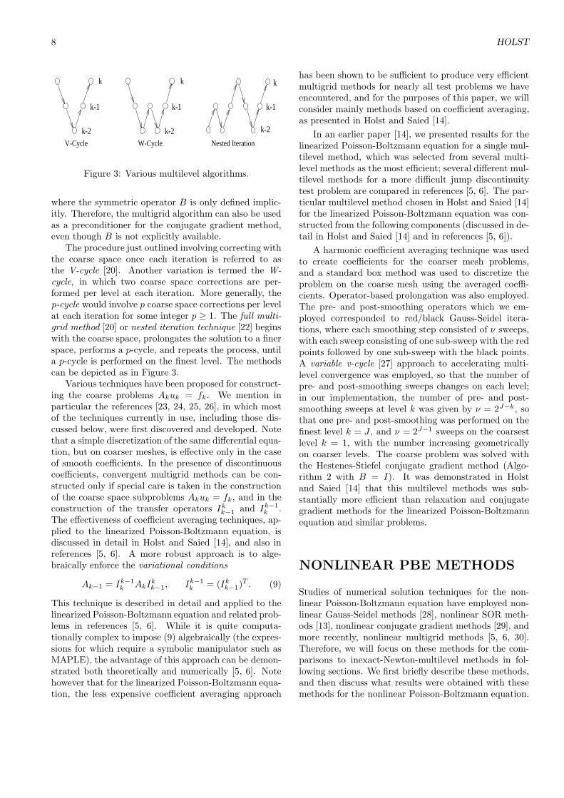
The procedure just outlined involving correcting withthe coarse space once each iteration is referred to asthe V-cycle [20]. Another variation is termed the W-cycle, in which two coarse space corrections are per-formed per level at each iteration. More generally, thep-cycle would involve p coarse space corrections per levelat each iteration for some integer p ≥ 1. The full multi-grid method [20] or nested iteration technique [22] beginswith the coarse space, prolongates the solution to a finerspace, performs a p-cycle, and repeats the process, untila p-cycle is performed on the finest level. The methodscan be depicted as in Figure 3.

Various techniques have been proposed for construct-ing the coarse problems Akuk = fk. We mention inparticular the references [23, 24, 25, 26], in which mostof the techniques currently in use, including those dis-cussed below, were first discovered and developed. Notethat a simple discretization of the same differential equa-tion, but on coarser meshes, is effective only in the caseof smooth coefficients. In the presence of discontinuouscoefficients, convergent multigrid methods can be con-structed only if special care is taken in the constructionof the coarse space subproblems Akuk = fk, and in theconstruction of the transfer operators Ik

k−1 and Ik−1k .

The effectiveness of coefficient averaging techniques, ap-plied to the linearized Poisson-Boltzmann equation, isdiscussed in detail in Holst and Saied [14], and also inreferences [5, 6]. A more robust approach is to alge-braically enforce the variational conditions

Ak−1 = Ik−1k AkIk

k−1, Ik−1k = (Ik

k−1)T . (9)

This technique is described in detail and applied to thelinearized Poisson-Boltzmann equation and related prob-lems in references [5, 6]. While it is quite computa-tionally complex to impose (9) algebraically (the expres-sions for which require a symbolic manipulator such asMAPLE), the advantage of this approach can be demon-strated both theoretically and numerically [5, 6]. Notehowever that for the linearized Poisson-Boltzmann equa-tion, the less expensive coefficient averaging approach

has been shown to be sufficient to produce very efficientmultigrid methods for nearly all test problems we haveencountered, and for the purposes of this paper, we willconsider mainly methods based on coefficient averaging,as presented in Holst and Saied [14].

In an earlier paper [14], we presented results for thelinearized Poisson-Boltzmann equation for a single mul-tilevel method, which was selected from several multi-level methods as the most efficient; several different mul-tilevel methods for a more difficult jump discontinuitytest problem are compared in references [5, 6]. The par-ticular multilevel method chosen in Holst and Saied [14]for the linearized Poisson-Boltzmann equation was con-structed from the following components (discussed in de-tail in Holst and Saied [14] and in references [5, 6]).

A harmonic coefficient averaging technique was usedto create coefficients for the coarser mesh problems,and a standard box method was used to discretize theproblem on the coarse mesh using the averaged coeffi-cients. Operator-based prolongation was also employed.The pre- and post-smoothing operators which we em-ployed corresponded to red/black Gauss-Seidel itera-tions, where each smoothing step consisted of ν sweeps,with each sweep consisting of one sub-sweep with the redpoints followed by one sub-sweep with the black points.A variable v-cycle [27] approach to accelerating multi-level convergence was employed, so that the number ofpre- and post-smoothing sweeps changes on each level;in our implementation, the number of pre- and post-smoothing sweeps at level k was given by ν = 2J−k, sothat one pre- and post-smoothing was performed on thefinest level k = J , and ν = 2J−1 sweeps on the coarsestlevel k = 1, with the number increasing geometricallyon coarser levels. The coarse problem was solved withthe Hestenes-Stiefel conjugate gradient method (Algo-rithm 2 with B = I). It was demonstrated in Holstand Saied [14] that this multilevel methods was sub-stantially more efficient than relaxation and conjugategradient methods for the linearized Poisson-Boltzmannequation and similar problems.

NONLINEAR PBE METHODS

Studies of numerical solution techniques for the non-linear Poisson-Boltzmann equation have employed non-linear Gauss-Seidel methods [28], nonlinear SOR meth-ods [13], nonlinear conjugate gradient methods [29], andmore recently, nonlinear multigrid methods [5, 6, 30].Therefore, we will focus on these methods for the com-parisons to inexact-Newton-multilevel methods in fol-lowing sections. We first briefly describe these methods,and then discuss what results were obtained with thesemethods for the nonlinear Poisson-Boltzmann equation.


Nonlinear relaxation methods

The classical linear methods discussed earlier, such asGauss-Seidel and SOR, can be extended in the obviousway to nonlinear algebraic equations of the form (3). Ineach case, the method can be viewed as a fixed-pointiteration:

un+1 = G(un).

Of course, implementations of these methods, which werefer to as nonlinear Gauss-Seidel and nonlinear SORmethods, now require the solution of a sequence of one-dimensional nonlinear problems for each unknown in onestep of the method. Since the one-dimensional nonlinearproblems are often solved with Newton’s method, thesemethods are also referred to as Gauss-Seidel-Newton andSOR-Newton methods, meaning that the Gauss-Seidelor SOR iteration is the main or outer iteration, whereasthe inner iteration is performed by Newton’s method.

The convergence properties of these types of meth-ods, as well as a myriad of variations and relatedmethods, are discussed in detail in Ortega and Rhein-boldt [31]. Note, however, that the same difficulty aris-ing in the linear case also arises here: as the problemsize is increased (the mesh size is reduced), these meth-ods converge more and more slowly. As a result, we willconsider alternative methods in a moment, such as non-linear conjugate gradient methods, nonlinear multilevelmethods, and finally inexact-Newton methods.

Nonlinear Gauss-Seidel is used by Allison et al. [28]for the nonlinear Poisson-Boltzmann equation, where anonlinear Gauss-Seidel procedure is developed for thefull nonlinear Poisson-Boltzmann equation, employing acontinuation method to handle the numerical difficultiescreated by the exponential nonlinearity. Polynomial ap-proximations of the exponential function are employed,and the degree of the polynomial is continued from de-gree one (linearized Poisson-Boltzmann equation) to de-gree nineteen. At each continuation step, the nonlin-ear Poisson-Boltzmann equation employing the weakernonlinearity is solved with nonlinear Gauss-Seidel itera-tion. The final degree nineteen solution is then used asan initial approximation for the full exponential nonlin-ear Poisson-Boltzmann equation, and nonlinear Gauss-Seidel is used to resolve the final solution. This proce-dure, while perhaps one of the first numerical solutionsproduced for the full nonlinear problem, is extremelytime-consuming.

An improvement is, as in the linear case, to employ anonlinear SOR iteration. The procedure works very wellfor the nonlinear Poisson-Boltzmann equation in manysituations and is extremely efficient [13]; unfortunately,there are cases where the iteration diverges [32, 13].In particular, it is noted on page 443 of Nicholls andHonig [13] that if the potential in the solvent (where theexponential term is evaluated) passes a threshold value

of seven or eight, then the nonlinear SOR method theypropose diverges. We will present some experiments witha nonlinear SOR iteration, provided with an experimen-tally determined near optimal relaxation parameter, andimplemented with a red/black ordering and array ori-ented data structures for high performance.

Nonlinear conjugate gradient methods

Let A be an SPD matrix, B(·) a nonlinear mapping fromR

n into R, and let (·, ·) denote an inner-product in Rn.

The following minimization problem:

Find u ∈ Rn such that J(u) = min

v∈RnJ(v),

where

J(u) =1

2(Au, u) + B(u) − (f, u),

is equivalent to the associated zero-point problem:

Find u ∈ Rn such that F (u) = Au + N(u) − f = 0,

where N(u) = B′(u); this follows by simply differentiat-ing J(u) to obtain the gradient mapping F (·) associatedwith J(·). We will assume here that both problems areuniquely solvable. A more detailed discussion of convexfunctionals and their related gradient mappings can befound in references [5, 6].

An effective approach for solving the zero-point prob-lem, by exploiting the connection with the minimizationproblem, is the Fletcher-Reeves version [33] of the non-linear conjugate gradient method, which takes the form:

Algorithm 4 (Fletcher-Reeves Nonlinear CG)

Let u0 ∈ Rn be given.

r0 = f − N(u0) − Au0, p0 = r0.Do i = 0, 1, . . . until convergence:

αi = (see below)ui+1 = ui + αip

i

ri+1 = ri + N(ui) − N(ui+1) − αiApi

βi+1 = (ri+1, ri+1)/(ri, ri)pi+1 = ri+1 + βi+1p

i

End do.

The directions pi are computed from the previousdirection and the new residual, and the steplength αi

is chosen to minimize the associated functional J(·) inthe direction pi. In other words, αi is chosen to min-imize J(ui + αip

i), which is equivalent to solving theone-dimensional zero-point problem:

dJ(ui + αipi)

dαi= 0.

Given the form of J(·) above, we have that

J(ui + αipi) =

1

2(A(ui + αip

i), ui + αipi)

+B(ui + αipi) − (f, ui + αip

i)

10 HOLST

A simple differentiation with respect to αi (and somesimplification) gives:

dJ(ui + αipi)

dαi= αi(Api, pi) − (ri, pi)

+(N(ui + αipi) − N(ui), pi),

where ri = f − N(ui) − Aui is the nonlinear residual.The second derivative with respect to αi will be usefulalso, which is easily seen to be:

d2J(ui + αipi)

dα2i

= (Api, pi) + (N ′(ui + αipi)pi, pi).

Now, Newton’s method for solving the zero-point prob-lem for αi takes the form:

αm+1i = αm

i − δm

where

δm =dJ(ui + αm

i pi)/dαi

d2J(ui + αmi pi)/dα2

i

=αm

i (Api, pi) − (ri, pi) + (N(ui + αmi pi) − N(ui), pi)

(Api, pi) + (N ′(ui + αmi pi)pi, pi)

.

The quantities (Api, pi) and (ri, pi) can be computedonce at the start of each line search for αi, each requir-ing an inner-product (Api is available from the CG it-eration). Each Newton iteration for the new αm+1

i thenrequires evaluation of the nonlinear term N(ui + αm

i pi)and inner-product with pi, as well as evaluation of thederivative mapping N ′(ui + αip

i), application to pi, fol-lowed by inner-product with pi.

In the case that N(·) arises from the discretizationof a nonlinear partial differential equation and is of di-agonal form, meaning that the j-th component functionof the vector N(·) is a function of only the j-th compo-nent of the vector of nodal values u, or Nj(u) = Nj(uj),then the resulting Jacobian matrix N ′(·) of N(·) is a di-agonal matrix. This situation occurs with box-methoddiscretizations of the nonlinear Poisson-Boltzmann equa-tion and similar equations. As a result, computing theterm (N ′(ui + αip

i)pi, pi) can be performed with feweroperations than two inner-products.

The total cost for each Newton iteration (beyond thefirst) is then evaluation of N(·) and N ′(·), and some-thing less than three inner-products. Therefore, the linesearch can be performed fairly inexpensively in certainsituations. If alternative methods are used to solve theone-dimensional problem defining αi, then evaluation ofthe Jacobian matrix can be avoided altogether, althoughthe Jacobian matrix is cheaply computable in the par-ticular applications we are interested in here.

Note that if the nonlinear term N(·) is absent, thenthe zero-point problem is linear and the associated en-ergy functional is quadratic:

F (u) = Au − f = 0, J(u) =1

2(Au, u) − (f, u).

In this case, the Fletcher-Reeves CG algorithm reducesto exactly the Hestenes-Stiefel [15] linear conjugate gra-dient algorithm (Algorithm 2 discussed earlier, with thepreconditioner B = I). The exact solution to the linearproblem Au = f , as well as to the associated minimiza-tion problem, can be reached in no more than n steps,where n is the dimension of the space R

n (see Theo-rem 8.6.1 in Ortega and Rheinboldt [31]). The calcula-tion of the steplength αi no longer requires the iterativesolution of a one-dimensional minimization problem withNewton’s method, since:

dJ(ui + αipi)

dαi= αi(Api, pi) − (ri, pi) = 0

yields an explicit expression for the αi which minimizesthe functional J in the direction pi:

αi =(ri, pi)

(Api, pi).

In the recent paper of Luty et. al [29], a nonlinearconjugate gradient method is applied to the nonlinearPoisson-Boltzmann equation. The conclusions of theirstudy were that the Fletcher-Reeves variant of the non-linear conjugate gradient method, which is the naturalextension of the Hestenes-Stiefel algorithm they had em-ployed for the linearized Poisson-Boltzmann equation inan earlier study [18], was an effective technique for thenonlinear Poisson-Boltzmann equation. We note thatit is remarked on page 1117 of the paper by Luty etal. [29] that solution time for the nonlinear conjugategradient method on the full nonlinear problem is fivetimes greater than for the linear method applied to thelinearized problem. We will present experiments withthe standard Fletcher-Reeves nonlinear conjugate gra-dient method, Algorithm 4, which they employed. Ourimplementation is aggressively optimized for high per-formance.

Nonlinear multilevel methods

Fully nonlinear multilevel methods were developed origi-nally by Brandt [20] and Hackbusch [34]. These methodsattempt to avoid Newton-linearization by acceleratingnonlinear relaxation methods with multiple coarse prob-lems. We are again concerned with the problem:

F (u) = Au + N(u) − f = 0.


Let us introduce the notation M(·) = A + N(·), whichyields the equivalent problem:

M(u) = f.

Consider a nested sequence of finite-dimensional spacesR

n1 ⊂ Rn2 ⊂ · · · ⊂ R

nJ ≡ Rn, where R

nJ is the finestspace and R

n1 the coarsest space, each space being con-nected to the others via prolongation and restrictionoperators, exactly as in the linear case described ear-lier. The full approximation scheme [20] or the nonlinearmultigrid method [22] has the following form:

Algorithm 5 (Nonlinear Multilevel Method)

ui+1 = NML(J, ui, f)

where u1k = NML(k, u0

k, fk) is defined recursively:

IF (k = 1) THEN:(1) Solve directly: u1

1 = M−11 (f1).

ELSE:

(1) Restriction: uk−1 = Ik−1k u0

k,

rk−1 = Ik−1k (fk − Mk(u0

k)).(2) Coarse source term:

fk−1 = Mk−1(uk−1) − rk−1.(3) Coarse problem:

wk−1 = uk−1 − NML(k − 1, uk−1, fk−1).(4) Prolongation: wk = Ik

k−1wk−1.(5) Damping parameter: λ = (see below).(6) Correction: vk = u0

k + λwk.(7) Post-smoothing: u1

k = Sk(vk , fk).END.

The practical aspects of this algorithm and varia-tions are discussed by Brandt [20], and a convergencetheory has been developed by Hackbusch [22], and morerecently by Hackbusch and Reusken [35, 36, 37, 38].

Note that we have introduced a damping parameterλ in the coarse space correction step of Algorithm 5.In fact, without this damping parameter, the algorithmfails for difficult problems such as those with exponentialor rapid nonlinearities. To explain how the dampingparameter is chosen, we refer back to our discussion ofnonlinear conjugate gradient methods. We begin withthe following energy functional:

Jk(uk) =1

2(Akuk, uk)k + Bk(uk) − (fk, uk)k.

As we have seen, the resulting minimization problem:

Find uk ∈ Rnk such that Jk(uk) = min

vk∈Rnk

Jk(vk)

is equivalent to the associated zero-point problem:

Find uk ∈ Rnk such that Fk(uk) = 0,

where Fk(uk) = Akuk + Nk(uk) − fk = 0, and whereNk(uk) = B′

k(uk). In other words, Fk(·) is a gradient

mapping of the associated energy functional Jk(·), wherewe assume that both problems above are uniquely solv-able.

In Hackbusch and Reusken [36], it is shown undercertain conditions that the prolongated coarse space cor-rection wk = Ik

k−1wk−1 is a descent direction for thefunctional Jk(·), meaning that there exists some λ > 0such that

Jk(uk + λwk) < Jk(uk).

In other words, the nonlinear multigrid method can bemade globally convergent if a damping parameter λ isfound for each coarse grid correction. We can findsuch a λ by minimizing Jk(·) along the descent direc-tion wk, which is equivalent to solving the following one-dimensional problem:

dJ(uk + λwk)

dλ= 0.

As in the discussion of the nonlinear conjugate gradientmethod, the one-dimensional problem can be solved withNewton’s method:

λm+1 = λm −X

Y,

where (exactly as for the nonlinear CG method)

X = λm(Akwk, wk)k − (rk , wk)k + (Nk(uk + λmwk)

−Nk(uk), wk)k,

Y = (Akwk, wk)k + (N ′k(uk + λmwk)wk, wk)k.

Now, recall that the “direction” from the coarse spacecorrection has the form: wk = Ik

k−1wk−1. The expres-sions for X and Y then take the form:

X = λm(AkIkk−1wk−1, I

kk−1wk−1)k − (rk, Ik

k−1wk−1)k

+ (Nk(uk + λmIkk−1wk−1) − Nk(uk), Ik

k−1wk−1)k,

Y = (AkIkk−1wk−1, I

kk−1wk−1)k

+ (N ′k(uk + λmIk

k−1wk−1)Ikk−1wk−1, I

kk−1wk−1)k .

It is not difficult to show [36] that certain finite el-ement discretizations of the nonlinear elliptic problemwe are considering, on two successively refined meshes,satisfy the following so-called nonlinear variational con-ditions:

Ak−1 + Nk−1(·) = Ik−1k AkIk

k−1 + Ik−1k Nk(Ik

k−1·),

Ik−1k = (Ik

k−1)T . (10)

As in the linear case, these conditions are usually re-quired [35, 36] to show theoretical convergence resultsabout nonlinear multilevel methods. Unfortunately, un-like the linear case, there does not appear to be a way

12 HOLST

to enforce these conditions algebraically (at least for thestrictly nonlinear term Nk(·)) in an efficient way. There-fore, if we employ discretization methods other than fi-nite element methods, or cannot approximate the inte-grals accurately (such as if discontinuities occur withinelements on coarser levels) for assembling the discretenonlinear system, then the variational conditions will beviolated. There is then no guarantee that the coarse gridcorrection is a descent direction. In other words, in thepresence of coefficient discontinuities and/or non-finiteelement discretizations, the nonlinear multigrid methodmay not converge, and may not be a fully reliable, robustmethod.

Nonlinear multigrid methods have been consideredby Oberoi and Allewell [30] and in references [5, 6]for the nonlinear Poisson-Boltzmann equation. Forsimple Poisson-Boltzmann equation problems, it hasbeen shown to be an efficient method, and appearsto demonstrate O(n) complexity as does linear multi-grid [5, 6, 30]. However, experiments performed else-where (see references [5, 6]) and below indicate thateven a quite sophisticated implementation of nonlin-ear multigrid may diverge for difficult problems suchas the nonlinear Poisson-Boltzmann equation with com-plex, large, or highly charged molecules. The inexact-Newton-multilevel methods we propose in the next sec-tion overcome these difficulties, and converge even forthe most difficult problems.

The method we employ for our numerical experi-ments below is the nonlinear multilevel method pre-sented earlier as Algorithm 5. All components requiredfor this nonlinear method are as in the linear harmoni-cally averaged multilevel method described in Holst andSaied [14] and in Holst [5, 6], except for the followingrequired modifications. The pre- and post-smoothingiterations correspond to nonlinear Gauss-Seidel, whereeach smoothing step consisting of ν sweeps; as in thelinear case, we employ a variable v-cycle so that ν in-creases as coarser levels are reached. Nonlinear operator-based prolongation [5, 6] is also employed for nested it-eration; otherwise, linear operator-based prolongation isused. The coarse problem is solved with the nonlinearconjugate gradient method, and a damping parameter,as described earlier is required; otherwise, the methoddoes not converge for rapid nonlinearities such as thosepresent in the nonlinear Poisson-Boltzmann equation.

INEXACT-NEWTON

METHODS

Given the nonlinear operator F : D ⊂ Rn 7→ R

n, ageneralization of the classical one-dimensional Newton’smethod for solving the problem F (u) = 0 is as follows:

F ′(un)vn = −F (un) (11)

un+1 = un + vn, (12)

where F ′(un) is the Jacobian matrix of partial deriva-tives:

F ′(u) = ∇F (u)T =

[

∂Fi(u)

∂uj

]

,

where F (u) = (F1(u), . . . , Fm(u))T , and where the func-tion u = (u1, . . . , un)T . In other words, the Newtoniteration is simply a special fixed-point iteration:

un+1 = G(un) = un − F ′(un)−1F (un). (13)

There are several variations of the standard (or full)Newton iteration (11)–(12) commonly used for nonlinearalgebraic equations which we mention briefly. A quasi-Newton method refers to a method which uses an ap-proximation to the true Jacobian matrix for solving theNewton equations. A truncated-Newton method uses thetrue Jacobian matrix in the Newton iteration, but solvesthe Jacobian system only approximately, using an itera-tive linear solver in which the iteration is stopped earlyor truncated. Inexact- or approximate-Newton methodsrefers to all of these types of methods collectively, wherein the most general case an approximate Newton direc-tion is produced in some unspecified fashion.

The inexact-Newton approach is of interest for thenonlinear Poisson-Boltzmann equation for the followingreasons. First, in the case of problems such as the non-linear Poisson-Boltzmann equation, which consist of aleading linear term plus a nonlinear term which doesnot depend on derivatives of the solution, the nonlinearalgebraic equations generated by discretization have theform:

F (u) = Au + N(u) − f = 0.

The matrix A is SPD, and the nonlinear term N(·)is often simple, and in fact is often diagonal, meaningthat the j-th component of the vector function N(u)is a function of only the j-th entry of the vector u, orNj(u) = Nj(uj); this occurs for example in the case ofa box-method discretization of the Poisson-Boltzmannequation and similar equations. Further, it is often thecase that the derivative N ′(·) of the nonlinear term N(·),which will be a diagonal matrix due to the fact that N(·)is of diagonal form, can be computed (often analytically)at low expense. If this is the case, then the entire trueJacobian matrix is available at low cost, since :

F ′(u) = A + N ′(u).

For the nonlinear Poisson-Boltzmann equation, we havethat Ni(u) = Ni(ui) = meas(τ (i))κ(xi) sinh(ui), so thatthe contribution to the Jacobian can be computed ana-lytically:

N ′i (u) = N ′

i(ui) = meas(τ (i))κ(xi) cosh(ui).


A second reason for our interest in the inexact-Newton approach is that the efficient multilevel methodsfor the linearized Poisson-Boltzmann equation [5, 6, 14]can be used effectively for the Jacobian systems; this isbecause the Jacobian F ′(u) is essentially the linearizedPoisson-Boltzmann operator, where only the diagonalHelmholtz-like term N ′(·) changes from one Newton it-eration to the next. Our fast linear multilevel methodsshould be effective as inexact Jacobian system solvers,and this has been demonstrated numerically in earlierpapers [5, 6, 14] and will be again later in this paper.

The hope is that solving the Jacobian systems onlyapproximately (requiring perhaps a few more Newtoniterations due to the inexactness of the Newton direc-tion), using a fast linear multilevel method, will be lesscostly in terms of execution time than employing a fullNewton method (requiring fewer Newton iterations sincethe direction is exact), and solving the Jacobian systemsexactly at each iteration. We will see that this is thecase later in the paper, and in fact the inexact approachmay be substantially more efficient than the full Newtonapproach.

However, there are two important considerationswhen using an inexact Newton method. First, how “in-exactly” can one solve the Jacobian system and still con-verge at a desirably fast rate, and how can one enforceglobal convergence properties for the overall Newton it-eration, so that the method will be robust. We statemore precisely, and then answer, both of these ques-tions in the next two sections, and then present the re-sulting global inexact-Newton-multilevel method in thethird section.

Inexactness and superlinear convergence

Let u ∈ Rn. A sequence un is said to converge strongly

to u if limn→∞ ‖u − un‖ = 0. There are three basicimportant notions regarding the rate of convergence of asequence of iterates produce by Newton’s method, andwe state them below as definitions.

Definition 1 The sequence un converges Q-linearlyto u if there exists c ∈ [0, 1) and n ≥ 0 such that forn ≥ n,

‖u− un+1‖ ≤ c‖u − un‖.

Definition 2 The sequence un converges Q-super-linearly to u if there exists cn such that cn → 0 and:

‖u − un+1‖ ≤ cn‖u − un‖.

Definition 3 The sequence un converges at rate Q-order(p) to u if there exists p > 1, c ≥ 0, n ≥ 0 suchthat for n ≥ n,

‖u− un+1‖ ≤ c‖u − un‖p.

The following notion of continuity is also necessary.

Definition 4 The mapping F : D ⊂ Rn 7→ R

n is calledHolder-continuous on D with constant γ and exponent pif there exists γ ≥ 0 and p ∈ (0, 1] such that

‖F (u) − F (v)‖ ≤ γ‖u− v‖p ∀u, v ∈ D ⊂ H.

If p = 1, then F is called uniformly Lipschitz-continuouson D, with Lipschitz constant γ. If in addition γ < 1,then F is called a contraction mapping with contractionconstant γ.

If an initial approximation is close enough to thetrue solution u, then under certain conditions it can beshown that [39] that a full Newton’s method will con-verge, and do so Q-superlinearly. The convergence ratewill not be so advantageous if an inexact Newton methodis employed. However, it can be shown that the con-vergence behavior of these inexact-Newton methods issimilar to the standard Newton’s method, and Newton-Kantorovich-like theorems can be established (see Chap-ter 18 of Kantorovich and Akilov [39] and below).

In particular, Quasi-Newton methods are studied inDennis and More [40], and a “characterization” theoremis established for the sequence of approximate Jacobiansystems. This theorem establishes sufficient conditionson the sequence Bi, where Bi ≈ F ′, to ensure su-perlinear convergence of a quasi-Newton method. Aninteresting result which they obtained is that the “con-sistency” condition is not required, meaning that thesequence Bi need not converge to the true JacobianF ′(·) at the root of the equation F (u) = 0, and su-perlinear convergence can still be obtained. In a laterpaper [41], this characterization theorem is rephrased ina geometric form, showing essentially that the full ortrue Newton step must be approached, asymptotically,in both length and direction, to attain superlinear con-vergence in a quasi-Newton iteration.

Inexact-Newton methods are studied directly byDembo et al. [42]. Their motivation is the use of it-erative solution methods for approximate solution of thetrue Jacobian systems. They establish conditions on theaccuracy of the inexact Jacobian solves at each Newtoniteration which will ensure superlinear convergence. Theinexact-Newton method is analyzed in the form:

F ′(un)vn = −F (un) + rn,‖rn‖

‖F (un)‖≤ ηn,

un+1 = un + vn.

In other words, the quantity rn, which is simply theresidual of the Jacobian linear system, indicates the in-exactness allowed in the approximate linear solve, andis exactly what one would monitor in a linear itera-tive solver. It is established that if the forcing sequenceηn < 1 for all n, then the above method is locally con-vergent. Their main result is the following theorem.

14 HOLST

Theorem 2 Assume there exists a unique u such thatF (u) = 0, that the inexact-Newton iterates un con-verge to u, and that both F (·) and F ′(·) are sufficientlysmooth. Then:

1. The convergence is superlinear if: limn→∞ ηn = 0.

2. The convergence is at least Q-order(1+p) if F ′(u)is Holder continuous with exponent p, and

ηn = O(‖F (un)‖p), as n → ∞.

Proof. See Dembo et al. [42].

As a result of this theorem, they suggest the tolerancerule:

ηn = min

1

2, C‖F (un)‖p

, 0 < p ≤ 1, (14)

which guarantees Q-order convergence of at least 1 + p.

Inexactness and global convergence

As noted in the previous section, Newton-like methodsconverge if the initial approximation is “close” to the so-lution; different convergence theorems require differentnotions of closeness. If the initial approximation is closeenough to the solution, then superlinear or Q-order(p)convergence occurs. However, the fact that these the-orems require a good initial approximation is also indi-cated in practice: it is well known that Newton’s methodwill converge slowly or fail to converge at all if the initialapproximation is not good enough.

On the other hand, methods such as those usedfor unconstrained minimization can be considered to be“globally” convergent methods, although their conver-gence rates are often extremely poor. One approach toimproving the robustness of a Newton iteration withoutloosing the favorable convergence properties close to thesolution is to combine the iteration with a global min-imization method. In other words, we can attempt toforce global convergence of Newton’s method by requir-ing that:

‖F (un+1)‖ < ‖F (un)‖,

meaning that we require a decrease in the value of thefunction at each iteration. But this is exactly whatglobal minimization methods, such as the nonlinear con-jugate gradient method, attempt to achieve: progresstoward the solution at each step.

More formally, we wish to define a minimizationproblem, such that the solution of the zero-point prob-lem we are interested in also solves the associated mini-mization problem. Let us define the following two prob-lems:

P1: Find u ∈ Rn such that F (u) = 0.

P2: Find u ∈ Rn such that J(u) = minv∈Rn J(v),

where J(·) is a functional, mapping Rn into R. We as-

sume that Problem 2 has been defined so that the uniquesolution to Problem 1 is also the unique solution to Prob-lem 2; note that in general, there may not exist a naturalfunctional J(·) for a given F (·), although we will see ina moment that it is always possible to construct an ap-propriate functional J(·).

A descent direction for the functional J(·) at thepoint u is any direction v such that the directionalderivative of J(·) at u in the direction v is negative, or(J ′(u), v) < 0, where (·, ·) is an inner-product in R

n, andJ ′(·) is the derivative of the functional J(·):

J ′(u) = ∇J(u)T =

(

J(u)

∂u1, . . . ,

J(u)

∂un

)T

.

If v is a descent direction, then it is not difficult to show(Theorem 8.2.1 in Ortega and Rheinboldt [31]) there ex-ists λ > 0 such that:

J(u + λv) < J(u). (15)

This follows from a generalized Taylor expansion (cf.page 255 in Kesavan [43]), since

J(u + λv) = J(u) + λ(J ′(u), v) + O(λ2).

If λ is sufficiently small and (J ′(u), v) < 0 holds (v isa descent direction), then clearly J(u + λv) < J(u). Inother words, if a descent direction can be found at thecurrent solution un, then an improved solution un+1 canbe found for some steplength in the descent direction v;i.e., by performing a one-dimensional line search for λuntil (15) is satisfied.

Therefore, if we can show that the Newton directionis a descent direction, then performing a one-dimensionalline search in the Newton direction will always guaranteeprogress toward the solution. In the case that we definethe functional as:

J(u) =1

2‖F (u)‖2 =

1

2(F (u), F (u)),

we can show that the Newton direction is a descent direc-tion. While the following result is easy to show for R

n,it is also true in the general case of a Hilbert space [5, 6]when ‖ · ‖ = (·, ·)1/2:

J ′(u) = F ′(u)T F (u).

The Newton direction at u is simply v = −F ′(u)−1F (u),so if F (u) 6= 0, then:

(J ′(u), v) = −(F ′(u)T F (u), F ′(u)−1F (u))

= −(F (u), F (u)) < 0.

Therefore, the Newton direction is always a descent di-rection for this particular choice of J(·), and by the in-troduction of the damping parameter λ, the Newton it-eration can be made globally convergent in the abovesense.


Consider now the inexact Newton method; since onlythe exact Newton direction is known to be a descent di-rection, we have no assurance that the inexact directionwill give descent, so the global properties gained by adamping parameter are lost. We can still attempt to in-troduce the damping parameter λ as before, so that theresulting algorithm for solving F (u) = 0 is:

Algorithm 6 (Damped-Inexact-Newton Method)

F ′(un)vn = −F (un) + rn,‖rn‖

‖F (un)‖≤ ηn,

un+1 = un + λnvn,

where we have left as unspecified how “large” the resid-ual rn is allowed to be, and how the damping parametersλn are chosen.

The following theorem from references [5, 6] givesa necessary and sufficient condition on the residual rn

of the Jacobian system system for the resulting inexactNewton direction to be a descent direction. This willallow us to use the damping parameter to achieve globalconvergence properties in the inexact-Newton algorithm.

Theorem 3 Inexact-Newton (Algorithm 6) yields a de-scent direction v at u if and only if the residual of theJacobian system, r = F ′(u)v + F (u), satisfies:

(F (u), r) < (F (u), F (u)).

Proof. We remarked earlier that an equivalent minimiza-tion problem (appropriate for Newton’s method) to as-sociate with the zero point problem F (u) = 0 is givenby minu∈Rn J(u), where J(u) = (F (u), F (u))/2. Wealso noted that the derivative of J(u) can be written asJ ′(u) = F ′(u)T F (u). Now, the direction v is a descentdirection for J(u) if and only if (J ′(u), v) < 0. The exactNewton direction is v = −F ′(u)−1F (u), and as shownearlier is always a descent direction. Consider now theinexact direction satisfying:

F ′(u)v = −F (u) + r, or v = F ′(u)−1[r − F (u)].

This inexact direction is a descent direction if and onlyif:

(J ′(u), v) = (F ′(u)T F (u), F ′(u)−1[r − F (u)])

= (F (u), r − F (u))

= (F (u), r) − (F (u), F (u))

< 0,

which is true if and only if the residual of the Jacobiansystem r satisfies:

(F (u), r) < (F (u), F (u)).

This leads to the following simple sufficient condition fordescent.

Corollary 4 Inexact Newton (Algorithm 6) yields a de-scent direction v at the point u if the residual of the Ja-cobian system, r = F ′(u)v + F (u), satisfies:

‖r‖ < ‖F (u)‖.

Proof. From the proof of Theorem 3 we have:

(J ′(u), v) = (F (u), r) − (F (u), F (u))

≤ ‖F (u)‖‖r‖ − ‖F (u)‖2,

where we have employed the Cauchy-Schwarz inequality.Therefore, if ‖r‖ < ‖F (u)‖, then the rightmost term isclearly negative (unless F (u) = 0), so that v is a descentdirection.

The sufficient condition presented as Corollary 4 ap-pears in references [5, 6], and also as a lemma in [44].Note that most stopping criteria for the Newton iter-ation involve evaluating F (·) at the previous Newtoniterate un. The quantity F (un) will have been com-puted during the computation of the previous Newtoniterate un, and the tolerance for un+1 which guaranteesdescent requires (F (un), r) < (F (un), F (un)) by Theo-rem 3. This involves only the inner-product of r andF (un), so that enforcing this tolerance requires only anadditional inner-product during the Jacobian linear sys-tem solve, which for n unknowns introduces an addi-tional n multiplies and n additions. In fact, a schememay be employed in which only a residual tolerance re-quirement for superlinear convergence is checked untilan iteration is reached in which it is satisfied. At thispoint, the descent direction tolerance requirement canbe checked, and additional iterations will proceed withthis descent stopping criterion until it too is satisfied. Ifthe linear solver reduces the norm of the residual mono-tonically (such as any of the linear methods discussedearlier), then the first stopping criterion need not bechecked again.

In other words, this adaptive Jacobian system stop-ping criterion, enforcing a tolerance on the residual forlocal superlinear convergence and ensuring a descent di-rection at each Newton iteration, can be implementedat the same computational cost as a simple check on thenorm of the residual of the Jacobian system.

Alternatively, the sufficient condition given in Corol-lary 4 may be employed at no additional cost, sinceonly the residual norm need be computed, which is alsorequired to insure superlinear convergence using Theo-rem 2.

Inexact-Newton-MG for the PBE

Discretization of the nonlinear Poisson-Boltzmann equa-tion (1) with the box-method discussed earlier produces

16 HOLST

a set of n nonlinear algebraic equations in n unknownsof the form (3), which we repeat here:

F (u) = Au + N(u) − f = 0.

The “holy grail” for this problem is an algorithm which(1) always converges, and (2) has optimal complexity,which in this case means O(n).

As we have just seen, the inexact-Newton methodcan be made essentially globally convergent with the in-troduction of a damping parameter. In addition, closeto the root, inexact-Newton has at least superlinear con-vergence properties thanks to Theorem 2. If a methodwith linear convergence properties is used to solve theJacobian systems at each Newton iteration, and the com-plexity of the linear solver is the dominant cost of eachNewton iteration, then the complexity properties of thelinear method will determine the complexity of the re-sulting Newton iteration asymptotically. With an effi-cient inexact solver such as a multilevel method for theearly damped iterations, employing a more stringent tol-erance for the later iterations as the root is approached,a very efficient yet robust nonlinear iteration should re-sult; in fact, if the linear method behaves as O(n), thena superlinearly-convergent nonlinear iteration should aswell.

The idea here, motivated by the work of Bank andRose [45, 46], is to combine the robust damped inexact-Newton methods with the fast linear multilevel solversdeveloped by Holst and Saied [14] and Holst [5, 6] forthe inexact Jacobian system solves. Combination withlinear multilevel iterative methods for the semiconduc-tor problem has been considered by Bank and Rose [46],along with questions of complexity. In a paper of Bankand Rose [45], an analysis of inexact-Newton methodsis performed, where a damping parameter has been in-troduced. A quite sophisticated algorithm GLOBAL isconstructed, enforcing both global and superlinear con-vergence properties; the sufficient descent condition es-tablished above is implicitly imbedded in their algorithmGLOBAL.

We propose the following alternative globally conver-gent inexact-Newton algorithm which is easy to under-stand and implement, based on the simple necessary andsufficient descent conditions established in the previoussection.

Algorithm 7 (Damped-Inexact-Newton method)

(1) Inexact solve: F ′(un)vn = −F (un) + rn,TST (rn) = TRUE,

(2) Correction: un+1 = un + λnvn,

where λn and TST (rn) are defined as:

TST (rn) : IF: ‖rn‖ ≤ C‖F (un)‖p+1, C, p > 0,(local Q-order(1+p) convergence)

AND: (F (un), rn) < (F (un), F (un))(guaranteed descent)

THEN: TST ≡ TRUEELSE: TST ≡ FALSE.

λn: ‖F (un + λnvn)‖ ≤ ‖F (un)‖ by line search;Always possible if TST (rn) = TRUE.The full inexact-Newton step (λn = 1)is always tried first.

An alternative less expensive TST (rn) is as follows:

TST (rn) : IF: ‖rn‖ ≤ C‖F (un)‖p+1, C, p > 0,(local Q-order(1+p) convergence)

AND: ‖rn‖ < ‖F (un)‖(guaranteed descent)

THEN: TST ≡ TRUEELSE: TST ≡ FALSE.

In Algorithm 7, the second condition in the firstTST (·) procedure is the necessary and sufficient con-dition for the inexact-Newton direction to be a descentdirection, established in Theorem 3. The second con-dition in the alternate TST (·) procedure is the weakersufficient condition established in Corollary 4. Note that,in early iterations when Q-order(1+p) for p > 0 is notto be expected, just satisfying one of the descent condi-tions is (necessary and) sufficient for progress toward thesolution. Algorithm 7 decouples the descent and super-linear convergence conditions, and would allow for theuse of only the weakest possible test of (F (un), rn) <(F (un), F (un)) far from the solution, ensuring progresstoward the solution with the least amount of work perNewton step.

Note also that the Q-order(1+p) condition

‖rn‖ ≤ C‖F (un)‖p+1

does not guarantee a descent direction, so that it is in-deed important to satisfy the descent condition sepa-rately. The Q-order(1+p) condition will impose descentif

C‖F (un)‖p+1 < ‖F (un)‖,

which does not always hold. If one is close to the so-lution, so that ‖F (un)‖ < 1, and if C ≤ 1, then theQ-order(1+p) condition will imply descent. By this lastcomment, we see that if ‖F (un)‖ < 1 and C ≤ 1, thenthe full inexact-Newton step is a descent direction, andsince we attempt this step first, we see that our algorithmreduces to the algorithm studied by Dembo et al. [42]near the solution; therefore, Theorem 2 above applies toAlgorithm 7 near the solution without modification.

Note that due to the special form of the nonlin-ear operator arising in the discrete nonlinear Poisson-Boltzmann equation, the damping step can be imple-mented in a surprisingly efficient manner. During the


one-dimensional line search for the parameter λn, wecontinually check for satisfaction of the inequality:

‖F (un + λnvn)‖ < ‖F (un)‖.

The term on the right is available from the previous New-ton iteration. The term on the left, although it might ap-pear to involve computing the full nonlinear residual, infact can avoid the operator-vector product contributedby the linear term. Simply note that

F (un + λnvn) = A[un + λnvn] + N(un + λnvn) − f

= [Aun − f ] + λn[Avn] + N(un + λnvn).

The term [Aun−f ] is available from the previous Newtoniteration, and [Avn] need be computed only once at eachNewton step. Computing F (un+λnvn) for each dampingstep beyond the first requires only the “saxpy” operation[Aun −f ]+λn[Avn] for the new damping parameter λn,and evaluation of the nonlinear term at the new dampedsolution, N(un + λnvn).

For the numerical comparisons with other methods,we employ Algorithm 7, taking p = 1 and C = 1.0×10−2

in the procedure TST (·), using the less expensive, suf-ficient descent condition form of the TST (·) procedure.The Jacobian system is solved inexactly at each step tothe residual tolerance specified by TST (·) by employ-ing the linear multilevel we designed for the linearizedPoisson-Boltzmann equation [5, 6, 14]. The damping pa-rameters λn are selected by a standard line search tech-nique. The result is an extremely robust and efficientnumerical method for the nonlinear Poisson-Boltzmannequation, as we will see shortly.

SOME TEST PROBLEMS

We describe briefly the nonlinear Poisson-Boltzmannequation test problems which we use to numerically eval-uate and compare the methods which have been pro-posed for the nonlinear Poisson-Boltzmann equation.We also describe a test problem which has a rapid non-linearity and very large jump discontinuities in the co-efficients, which will be used to evaluate some of themultilevel techniques.

The nonlinear PBE

Consider a very broad range of possible temperaturesT ∈ [200K, 400K], a broad range of possible ionicstrengths Is ∈ [0, 10], and the following representativepolygonal domain:

Ω = [xmin, xmax] × [ymin, ymax] × [zmin, zmax],

where the diameter of Ω is on the order of 10o

A to 500o

A.We assume that the set of discrete charges x1, . . . ,xNm

representing the molecule lie well within the domain, andhence far from the boundary Γ of Ω. The nonlinearPoisson-Boltzmann equation for the dimensionless po-tential u(x) then has the form:

−∇ · (ε(x)∇u(x)) + κ(x) sinh(u(x))

= C

Nm∑

i=1

ziδ(x − xi), in Ω ⊂ R3,

u(x) =C

4πεw

Nm∑

i=1

[zie−κ(x)|x−xi|/

√εw ]/|x − xi|, on Γ,

where C = 4πe2c/k−1

B T−1, and εw = 80. We have em-ployed one of the known analytical solutions for the lin-earized problem to obtain the boundary condition on Γappearing above. As remarked earlier, this is commonlydone; see for example Tanford [4] or in references [5, 6]for more detailed discussions of analytical solutions.

It is easy to show [5, 6] that the problem coefficientssatisfy the following bounds for the given temperatureand ionic strength ranges:

1. 2 ≤ ε(x) ≤ 80.

2. 0 ≤ κ2(x) ≤ 127.0.

3. 5249.0 ≤ C ≤ 10500.0.

4. −1 ≤ zi ≤ 1.

The nonlinear Poisson-Boltzmann problem will then becompletely defined by specifying the following quantities:

• xmin, xmax, ymin, ymax, zmin, zmax; the domain.

• ε(x); the electrostatic molecular surface.

• κ(x); defined by ionic strength and exclusion layer.

• C; constant depending only on the temperature T .

• x1, . . . ,xNm; the charge locations.

• z1, . . . , zNm; the associated fractional charges.

For all of our molecule test problems, we use T = 298which determines the constant C; this is a common pa-rameter setting for these types of problems. The domaingeometry will be defined by the particular molecule, aswell as the parameters ε(x) and κ(x), although we mustspecify also the ionic strength Is to completely deter-mine κ(x). The charge locations and corresponding frac-tional charges will also be determined by the particularmolecule.

The test data is taken from the Brookhaven proteindatabank, with the help of the DELPHI and UHBD soft-ware packages (described below). The test moleculeschosen for our study of the nonlinear Poisson-Boltzmannequation are the following:

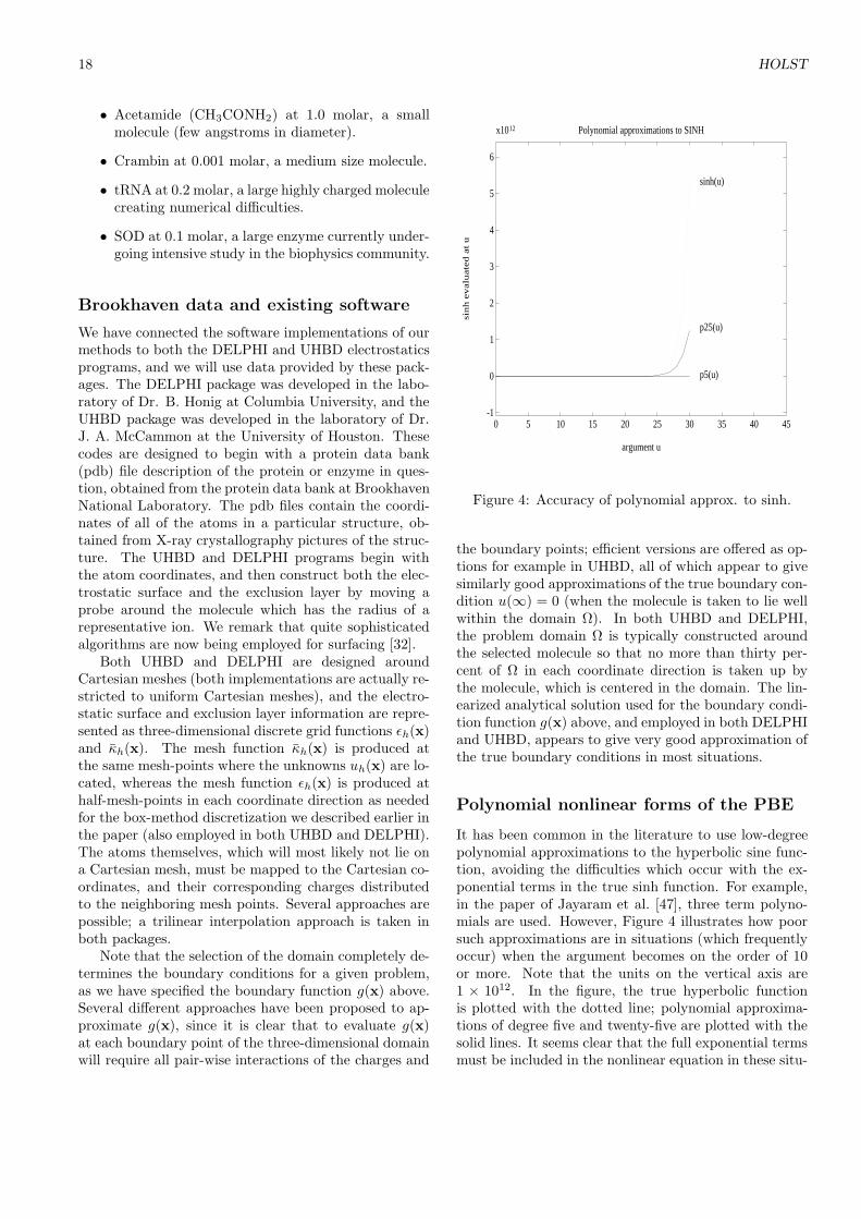
18 HOLST

• Acetamide (CH3CONH2) at 1.0 molar, a smallmolecule (few angstroms in diameter).

• Crambin at 0.001 molar, a medium size molecule.

• tRNA at 0.2 molar, a large highly charged moleculecreating numerical difficulties.

• SOD at 0.1 molar, a large enzyme currently under-going intensive study in the biophysics community.

Brookhaven data and existing software

We have connected the software implementations of ourmethods to both the DELPHI and UHBD electrostaticsprograms, and we will use data provided by these pack-ages. The DELPHI package was developed in the labo-ratory of Dr. B. Honig at Columbia University, and theUHBD package was developed in the laboratory of Dr.J. A. McCammon at the University of Houston. Thesecodes are designed to begin with a protein data bank(pdb) file description of the protein or enzyme in ques-tion, obtained from the protein data bank at BrookhavenNational Laboratory. The pdb files contain the coordi-nates of all of the atoms in a particular structure, ob-tained from X-ray crystallography pictures of the struc-ture. The UHBD and DELPHI programs begin withthe atom coordinates, and then construct both the elec-trostatic surface and the exclusion layer by moving aprobe around the molecule which has the radius of arepresentative ion. We remark that quite sophisticatedalgorithms are now being employed for surfacing [32].

Both UHBD and DELPHI are designed aroundCartesian meshes (both implementations are actually re-stricted to uniform Cartesian meshes), and the electro-static surface and exclusion layer information are repre-sented as three-dimensional discrete grid functions εh(x)and κh(x). The mesh function κh(x) is produced atthe same mesh-points where the unknowns uh(x) are lo-cated, whereas the mesh function εh(x) is produced athalf-mesh-points in each coordinate direction as neededfor the box-method discretization we described earlier inthe paper (also employed in both UHBD and DELPHI).The atoms themselves, which will most likely not lie ona Cartesian mesh, must be mapped to the Cartesian co-ordinates, and their corresponding charges distributedto the neighboring mesh points. Several approaches arepossible; a trilinear interpolation approach is taken inboth packages.

Note that the selection of the domain completely de-termines the boundary conditions for a given problem,as we have specified the boundary function g(x) above.Several different approaches have been proposed to ap-proximate g(x), since it is clear that to evaluate g(x)at each boundary point of the three-dimensional domainwill require all pair-wise interactions of the charges and

-1

0

1

2

3

4

5

6

x1012

0 5 10 15 20 25 30 35 40 45

argument u

sinh e

valu

ate

d a

t u

Polynomial approximations to SINH

sinh(u)

p5(u)

p25(u)

Figure 4: Accuracy of polynomial approx. to sinh.

the boundary points; efficient versions are offered as op-tions for example in UHBD, all of which appear to givesimilarly good approximations of the true boundary con-dition u(∞) = 0 (when the molecule is taken to lie wellwithin the domain Ω). In both UHBD and DELPHI,the problem domain Ω is typically constructed aroundthe selected molecule so that no more than thirty per-cent of Ω in each coordinate direction is taken up bythe molecule, which is centered in the domain. The lin-earized analytical solution used for the boundary condi-tion function g(x) above, and employed in both DELPHIand UHBD, appears to give very good approximation ofthe true boundary conditions in most situations.

Polynomial nonlinear forms of the PBE

It has been common in the literature to use low-degreepolynomial approximations to the hyperbolic sine func-tion, avoiding the difficulties which occur with the ex-ponential terms in the true sinh function. For example,in the paper of Jayaram et al. [47], three term polyno-mials are used. However, Figure 4 illustrates how poorsuch approximations are in situations (which frequentlyoccur) when the argument becomes on the order of 10or more. Note that the units on the vertical axis are1 × 1012. In the figure, the true hyperbolic functionis plotted with the dotted line; polynomial approxima-tions of degree five and twenty-five are plotted with thesolid lines. It seems clear that the full exponential termsmust be included in the nonlinear equation in these situ-


ations, which occur even in the case of lysozyme [32]. Insome sense it is a mute point, since our global inexact-Newton-multilevel methods control the numerical prob-lems of the exponential nonlinearity well, and for imple-mentation reasons (the intrinsic exponential functionsare much faster than a loop which evaluates a polyno-mial) the polynomial nonlinearity solution actually takeslonger to compute numerically with our methods (andother methods, when they converge for the exponentialcase) than the full exponential case. Therefore, we willconsider only the more correct exponential model.

A nonlinear jump discontinuity problem

The following test problem will be used to explore theconvergence behavior of the multilevel methods. Thedomain is the unit cube:

Ω = [0, 1]× [0, 1] × [0, 1].

The nonlinear equation has the form:

−∇ · (a(x)∇u(x)) + b(x, u(x)) = f(x) in Ω ⊂ R3,

u(x) = g(x) on Γ. (16)

where the coefficients in equation (16) are taken to be:

1. a : Ω 7→ L(R3), aij(x) = δijε(x), 1 ≤ ε(x) ≤ 103.

2. b : Ω × R 7→ R, b(x, u(x)) = λeu(x), λ ≥ 0.

3. f : Ω 7→ R, − 1 ≤ f(x) ≤ 1.

4. g : Γ 7→ R, g(x) = 0.

We will construct ε(x) to be piecewise constant, takingone value in a subdomain Ω1 ⊂ Ω, and a second value inthe region Ω\Ω1, so that ε(x) is defined as follows:

ε(x) =

1 ≤ ε1 ≤ 1.0 × 103 if x ∈ Ω1,1 ≤ ε2 ≤ 1.0 × 103 if x ∈ Ω\Ω1.

We will take ε1 and ε2 to be quite different in magnitude,so that their ratio:

D =ε1ε2

will be 103 or 10−3, similar to the nonlinear Poisson-Boltzmann equation. (Additional experiments were per-formed by Holst [5, 6], taking D to be be as large as 108

or as small as 10−8, and the resulting convergence behav-ior of the various methods was analyzed in detail.) Wedefine the subdomain Ω1 ⊂ Ω to consist of the followingtwo smaller cubes:

Ω1 = [0.25, 0.50]× [0.25, 0.50]× [0.25, 0.50]

∪ [0.50, 0.75]× [0.50, 0.50]× [0.50, 0.75].

Table 1: Nonlinear PBE methods.

Method Description

DINMH damped-inexact-Newton-MHDFNMH damped-full-Newton-MHNMH nonlinear MHNCG nonlinear CG (Fletcher-Reeves)NSOR nonlinear SOR (1-D Newton)NGS nonlinear Gauss-Seidel (1-D Newton)

For this simple problem, it would of course be possi-ble to construct all coarse meshes as needed for the mul-tilevel methods to align with Ω1; this would not possiblewith problems such as the nonlinear Poisson-Boltzmannequation and a complex molecule. Therefore, since wewish to simulate the case that the discontinuities in ε(x)cannot be resolved on coarser meshes, the multiple lev-els of tessellations of Ω into discrete meshes Ωk are con-structed so that the discontinuities in ε(x) lie along meshlines only on the finest mesh. In addition, we employa non-uniform Cartesian mesh, as shown in Figure 1,which attempts to provide a more accurate descriptionof the discontinuity interface on the finest mesh.

Note that if ε1 = ε2 ≡ 1, then problem (16) withthe above coefficients is the Bratu problem (see page432 in Davis [48] for information about this interestingproblem) on the unit cube.

NUMERICAL COMPARISONS

The global inexact-Newton-multilevel method presentedearlier is investigated numerically when applied to thenonlinear Poisson-Boltzmann equation and to a non-linear test problem with large jump discontinuities inthe coefficients and exponential nonlinearity. A detailedcomparison to other methods is presented, includingcomparisons to the classical nonlinear multigrid method,the nonlinear conjugate gradient method, and nonlin-ear relaxation methods such as SOR. Our results indi-cate that the two multilevel-based methods are supe-rior to the relaxation and conjugate gradient methods,and that the advantage of the multilevel-based methodsgrows with the problem size. In addition, experimentsindicate that the inexact Newton-multilevel approach isthe most efficient and robust method for the test prob-lems, and in particular is both more efficient and morerobust than the nonlinear multigrid method.

Table 1 provides a key to the plots and tables tofollow. For reference, at times we also will refer to thelinear methods in Table 2. Unless otherwise indicated,all data in the plots and tables to follow include the pre-processing costs incurred by the various methods. In

20 HOLST

Table 2: Some linearized PBE methods.

Method Description

MH harmonically averaged MG [14]MICCG modified incomplete Cholesky CG [14]DSCG diagonally preconditioned CG [14]

other words, the multilevel methods times include theadditional time required to set up the problem on coarsegrids. This gives a complete and fair assessment of thetotal time required to reach the solution.

An initial approximation of zero was taken to starteach method, and each method used a stopping criteriabased on the norm of the nonlinear function:

‖F (ui)‖ < TOL = 1.0e− 9,

where ui represents the ith iterate, and F (·) is thediscrete nonlinear algebraic operator for the equationF (u) = 0 which we are trying to solve. Of course, thisis not the most appropriate stopping criteria for nonlin-ear iterations (more appropriate stopping tests are dis-cussed in detail in references [5, 6]), but for our testproblems this test does indicate well when the solutionis approached, and it is the best approach for comparingdifferent methods since it guarantees that each methodis producing a solution of the same quality.

We remark that it was required to perform all com-putations in double precision; this is necessitated by therapid nonlinearities present in the equations, which re-sult an extreme loss in precision. Note that calculationsin double precision are more costly than single precisioncalculations, and so the execution times reported herefor some of the methods will be somewhat longer thansome of the single precision times reported in earlier pa-pers [5, 6, 14]

Timing figures on the Convex C240 and the Con-vex C3 were obtained from the system timing routinegetrusage. A more detailed performance analysis onseveral more sequential as well as some parallel machinescan be found in references [5, 6].

Results for acetamide

Figure 6 compares the methods in Table 1 for the ac-etamide problem. For this problem, all of the methodsconverge, and the two multilevel-based algorithms aresuperior. The nonlinear conjugate gradient and nonlin-ear SOR methods have comparable performance. Themethod DINMH is extremely efficient, representing animprovement of more than a factor of fifty over the non-linear SOR and nonlinear conjugate gradient methods,and a factor of ten over the nonlinear multigrid methodNMH.

Results for crambin

Figure 5 compares the methods in Table 1 for the cram-bin problem. Again, all of the methods converge, andthe two multilevel-based algorithms are superior. Thenonlinear conjugate gradient shows superiority to thenonlinear relaxation methods. The method DINMH isagain extremely efficient, representing an improvementof more than a factor of fifty over the nonlinear conjugategradient method, and a factor of ten over the nonlinearmultigrid method NMH.

Results for tRNA

We included this test problem because it appears tocause severe difficulties for other methods which havebeen tried; in fact, the nonlinear SOR procedure pro-posed by Nicholls and Honig [13] was known to di-verge for this problem [32]. However, we note thattheir method was not a true SOR-Newton iteration, andwas instead a fixed-point iteration based on a certainsplitting of the operator (see page 443 in Nicholls andHonig [13]). When a true SOR-Newton iteration is em-ployed, the method converges for this problem. Figure 7shows the relative performance of the various methods.Again, the method DINMH is the most efficient by farof the methods presented, representing a factor of fiftyimprovement over the next best method.

Note that for this problem, the nonlinear multilevelmethod diverges, even with linesearch for a damping pa-rameter. Since we do not enforce the nonlinear varia-tional conditions exactly, as outlined earlier and in moredetail in references [5, 6], we have no guarantee thatthe coarse level correction is a descent direction, and sothis method is not a global method; this particular testproblem illustrates this fact. It also shows that nonlin-ear multigrid method NMH is not only less robust thanDINMH, but also less reliable than NSOR and NCG.

Results for SOD

Figure 8 shows only two methods applied to the superox-ide dismutase (SOD) test problem: the method DINMHapplied to the full nonlinear Poisson-Boltzmann equa-tion; and the linear DSCG method applied to the lin-earized Poisson-Boltzmann equation. All other nonlin-ear methods studied here diverged for this test problem.Again, the method DINMH converges very rapidly, andthe superlinear convergence is clearly visible.

We have included the plot of the linear methodDSCG to show clearly that the DINMH method, solv-ing the full nonlinear problem, is more than a factor oftwo times more efficient than one of the best availablemethods in the literature for only the linearized problem.


0 100 200 300 400 500

10-12

10-10

10-8

10-6

10-4

10-2

100

102

Nonlinear Poisson-Boltzmann Equation MethodsMolecule: CRM

DINMH

NMH NCG NSOR

NGS (1490)

CPU Seconds

Rela

tive

Resid

ual

Convex C240 (1 Processor) with 31x31x31 Grid

Figure 5: Comparison of various methods for the nonlinear crambin problem.

0 200 400 600 800 1000 1200

10-10

10-8

10-6

10-4

10-2

100

102

Nonlinear Poisson-Boltzmann Equation MethodsMolecule: Acetemide

DINMH NMH NCG NSOR

CPU Seconds

Rela

tive

Resid

ual


Figure 6: Comparison of various methods for the nonlinear acetamide problem.

22 HOLST

0 200 400 600 800 1000 1200

10-12

10-10

10-8

10-6

10-4

10-2

100

102

Nonlinear Poisson-Boltzmann Equation MethodsMolecule: tRNA

DINMH

NMH

NCG (> 10,000)

NSOR

CPU Seconds

Rela

tive

Resid

ual


Figure 7: Comparison of various methods for the nonlinear tRNA problem.

0 200 400 600 800 1000 1200 1400 1600

10-14

10-12

10-10

10-8

10-6

10-4

10-2

100 Nonlinear Poisson-Boltzmann Equation Methods.

Test Molecule: SOD.

DINMH

DSCG(linearized PBE)

CPU seconds

Rela

tive

Resid

ual

Convex C3 with 127x127x127 Grid

Figure 8: Comparison of various methods for the nonlinear SOD problem.


Jump discontinuity problem results

Figure 9 shows the behavior of the five methods in Ta-ble 1 when applied to the jump discontinuity dest prob-lem, with D = ε1/ε2 = 10−3. The three multilevel-basedmethods are substantially superior to the nonlinear re-laxation and conjugate gradient methods. More interest-ingly, the comparison between the full Newton method(DFNMH) and the inexact Newton method (DINMH)shows at least a factor of four improvement gained byemploying the inexactness strategy outlined earlier (andcan be found in more detail in references [5, 6]).

Figure 10 shows the first 200 CPU seconds of Fig-ure 9 expanded to the whole axis. We have includedthe linear methods MH, MICCG, and DSCG on the plotto illustrate more graphically how efficient the methodDINMH is; it requires less than a factor of two timesmore CPU seconds than the linear method MH for thelinearized problem, and is a factor of two times more ef-ficient than the next best linear method, MICCG withvectorizable orderings (operating at near peak efficiencyon the Convex C3, which is a vector processor).

Storage requirements

We make a few remarks about the storage required forthe multilevel methods as well as some of the other meth-ods appearing in this paper. We are faced with the dis-crete problem of the form:

Au + N(u) = f,

where A is an n × n SPD matrix, N(·) is a nonlinearfunction mapping R

n into Rn, u is the n × 1 vector of

unknowns, and f is the n × 1 vector of source functionvalues. The number of unknowns n is related to the orig-inal discrete mesh as n = I ·J ·K, where I , J , and K arethe number of mesh-points in each direction of the Carte-sian mesh. Employing the box-method on the Cartesianmesh, the matrix A can be represented by seven diago-nals, only four of which need be stored in arrays of lengthn, due to the symmetry of A. The box-method produces“diagonal” nonlinear functions N(·) from the types ofnonlinear partial differential equations we consider inthis paper, and N(·) can be represented by a single realnonlinear function and a coefficient array of length n.Therefore, simply to store the nonlinear algebraic prob-lem on the finest desired (possibly non-uniform) Carte-sian mesh requires approximately 4n+1n+1n+1n = 7n.The nonlinear iterative algorithms we have consideredhere require various amounts of additional storage forimplementation.

With regard to multilevel methods, since the numberof unknowns drops by a factor of eight as one moves to acoarser mesh in three dimensions if standard successivelyrefined non-uniform Cartesian meshes are used, we see

that the storage required to represent on all meshes avector having length n on the finest mesh is:

n +n

8+

n

64+ · · · = n ·

(

1

8+

1

64+ · · ·

)

≤8

7· n.

We will assume that enough levels are always used sothat not only is the coarse problem computational costnegligible, but also the storage requirement (includingpossibly direct factorization of the matrix) is negligibledue to the size of the coarse problem.

Table 3 gives the required storage for a selection ofmethods. These figures reflect the storage requirementsin our implementations; in particular, while the NGS,NSOR, and NCG storage requirements are minimal orclose to minimal, the storage requirements for our multi-level methods could be reduced somewhat. To maintaina logically modular structure in our implementations, wehave allowed some redundant storage in the implementa-tions. In the methods NMH and DINMH, it is possibleto implement the (linear or nonlinear) operator-basedprolongation Ik

k−1 completely in terms of the matrix A(and the nonlinearity N(·)), without requiring explicitstorage of Ik

k−1. This can save 27n/7 ≈ 4n, which makesthese methods almost equivalent to NCG in terms ofstorage requirements, with NMH and DINMH requiringapproximately 13.7n and 16n, respectively.

Therefore, as in the case of the linear multilevelmethods presented in Holst and Saied [14] and in ref-erences [5, 6], not only do the multilevel methods dis-cussed here demonstrate superior complexity properties,we see that they can be implemented with very efficientmemory use, requiring the same or only slightly morestorage than that required for competing methods suchas nonlinear conjugate gradient methods.

CONCLUSIONS

We have shown numerically that the multilevel-basedmethods discussed in this paper are generally more ef-ficient than existing methods for the nonlinear Poisson-Boltzmann equation for a range of test molecules, andfor a difficult test problem with large coefficient discon-tinuities and rapid nonlinearity. In addition, our resultsindicate that the damped-inexact-Newton-multilevel ap-proach is not only the most efficient approach for theseproblems, but is also the most robust of all the meth-ods considered. It converged in all situations, and forthe SOD test problem was the only nonlinear method toconverge.

Regarding the nonlinear multigrid method, both the-oretical and numerical evidence here and elsewhere [5, 6]suggests that without careful use of special techniquesfor constructing the coarse problems (discussed in Holstand Saied [14] and Holst [5, 6]), and without the use

24 HOLST

0 100 200 300 400 500 600 70010

-14

10-12

10-10

10-8

10-6

10-4

10-2

100

Nonlinear jump discontinuity test problem.Discontinuity ratio (e1/e2) = 1.0e-03

CPU Seconds

Nonl

inea

r Rel

ative

Res

idua

lConvex C3 (1 Processor) with 65x65x65 Grid

DINMHDFNMH

NMH

NSOR

NCG (> 2550)

Figure 9: Comparison of methods for the nonlinear discontinuity problem.

0 50 100 150 20010

-14

10-12

10-10

10-8

10-6

10-4

10-2

100

Nonlinear jump discontinuity test problem.Discontinuity ratio (e1/e2) = 1.0e-03

CPU Seconds

Nonl

inea

r Rel

ative

Res

idua

l


DINMH

DFNMH

NMH

MH (linear)

MICCG (linear)

DSCG (linear)

Figure 10: Enlargement of previous figure, with linear methods added.


Table 3: Storage required by various nonlinear (and some linear) elliptic solvers.

Method Storage RequirementsName A N(·) u f Ik

k−1 WORK TOTAL

NGS 4n 1n 1n 1n 0n 1n 8nNSOR 4n 1n 1n 1n 0n 1n 8nNCG 4n 1n 1n 1n 0n 6n 13nNMH 4n + 4

7n 1n + 17n 1n + 1

7n 1n + 17n 27

7 n 5n + 57n ≈ 17.6n

DINMH 4n + 47n 1n + 1

7n 1n + 17n 1n + 1

7n 277 n 7n + 7

7n ≈ 19.9n

of a damping parameter, nonlinear multigrid methodsare inherently non-reliable (may not converge) for prob-lems with exponential nonlinearities and large coefficientdiscontinuities, such as the nonlinear Poisson-Boltzmannequation and equations occurring in semiconductor mod-eling.

We believe that this was not observed in the studyof Oberoi and Allewell [30] due to the small number ofexamples considered. In fact, they did not seem to re-quire either the damping parameter or the coefficientaveraging techniques built into the method NMH em-ployed here. Our experiments with such a “vanilla”nonlinear multigrid method showed divergence exceptfor the simplest possible molecules (acetamide) at verylow ionic strengths (Is < 0.0001) and small mesh sizes(31 × 31 × 31). To obtain convergence even for thecrambin case (Figure 5) required both the harmoniccoefficient averaging approach developed in Holst andSaied [14] and the damping parameter discussed earlierin this paper. We are not aware of other techniques forincreasing the robustness of nonlinear multigrid, with-out sacrificing most of the efficiency of the multilevelapproach.

The damped inexact-Newton-multilevel method ap-pears to be the most robust of all methods that have beenproposed; it converges for all cases we have encountered(this behavior is supported by the theory presented inthis paper, which was used to construct the method),and in particular it converges for cases which cause allother proposed methods to fail. In addition, it appearsto be substantially more efficient than all other meth-ods that have been proposed (by orders of magnitudefor some test problems), and is even more efficient thansome of the best existing linear methods producing onlya linearized solution.

These considerations demonstrate that the dampedinexact-Newton-multilevel method presented in this pa-per not only makes the nonlinear model completely fea-sible by providing a very reliable solution technique, butit actually improves on the efficiency of available linearalgorithms which are currently used for the less accuratelinear model. We remark that initial numerical experi-ments with larger mesh sizes show that the improvement

of the damped-inexact-Newton-multilevel approach overmethods grows with the problem size [49].

ACKNOWLEDGMENTS

The author thanks Dr. Saied at the University of Illi-nois, who supervised much of this work. Thanks arealso due to Dr. Kerkhoven, Dr. Saylor, and Dr. Skeelin the Computer Science Department at the Universityof Illinois, for many helpful discussions on the mate-rial in this paper. Dr. Subramaniam and Dr. Kozackof the Beckmann Institute at the University of Illinoisprovided helpful advice regarding the biophysical as-pects of this work. Dr. Nicholls of Columbia Univer-sity made much effort to supply the author with themolecule data for testing, and made available his ex-perience with this problem and his expertise with theelectrostatics program DELPHI, developed in the labo-ratory of Dr. Honig. Dr. McCammon and his groupin the Department of Chemistry at the University ofHouston made available the UHBD (University of Hous-ton Brownian Dynamics) software package, which al-lowed us to access additional data from the Brookhavenprotein databank. The National Center for Supercom-puter Applications, located at the University of Illinoisat Urbana-Champaign, provided access to the Cray Y-MP and the Convex C3 through support by the NationalScience Foundation. Access to the Convex C240 was pro-vided by the Computing Services Organization, also atthe University of Illinois at Urbana-Champaign.

This work was performed at the University of Illi-nois and at the California Institute of Technology, andwas supported in part by Department of Energy GrantNo. DOE DE-FG02-91ER25099, and in part by the NSFunder Cooperative Agreement No. CCR-9120008.

REFERENCES

[1] P. Debye and E. Huckel, Physik. Z., 24, 185 (1923).

[2] J. M. Briggs and J. A. McCammon, Computers inPhysics, 6 (3), 238–243 (1990).

26 HOLST

[3] K. A. Sharp and B. Honig, Annu. Rev. Biophys.Biophys. Chem., 19, 301–332 (1990).

[4] C. Tanford, Physical Chemistry of Macromolecules,John Wiley & Sons, New York, NY, 1961.

[5] M. Holst, tech. rep., Department of Applied Math-ematics and CRPC, California Institute of Technol-ogy, 1994.

[6] M. Holst, PhD thesis, Numerical ComputingGroup, Department of Computer Science, Univer-sity of Illinois at Urbana-Champaign, 1993. Alsopublished as Tech. Rep. UIUCDCS-R-03-1821.

[7] R. S. Varga, Matrix Iterative Analysis, Prentice-Hall, Englewood Cliffs, NJ, 1962.

[8] G. Strang and G. Fix, An Analysis of the FiniteElement Method, Prentice-Hall, Englewood Cliffs,NJ, 1973.

[9] E. L. Wachspress, Iterative Solution of Elliptic Sys-tems and Applications to the Neutron DiffusionEquations of Reactor Physics, Prentice-Hall, Engle-wood Cliffs, NJ, 1966.

[10] R. E. Bank and D. J. Rose, SIAM J. Numer. Anal.,24 (4), 777–787 (1987).

[11] T. Kerkhoven, SIAM J. Numer. Anal., (1992). (Toappear).

[12] J. M. Ortega, Numerical Analysis: A SecondCourse, Academic Press, New York, NY, 1972.

[13] A. Nicholls and B. Honig, J. Comput. Chem.,12 (4), 435–445 (1991).

[14] M. Holst and F. Saied, J. Comput. Chem.,14 (1), 105–113 (1993).

[15] M. R. Hestenes and E. Stiefel, J. Research of NBS,49, 409–435 (1952).

[16] P. Concus, G. H. Golub, and D. P. O’Leary, inSparse Matrix Computations, J. R. Bunch and D. J.Rose, eds., Academic Press, New York, NY, 1976,pp. 309–332.

[17] S. F. Ashby, T. A. Manteuffel, and P. E. Saylor,Tech. Rep. UCRL-98508, Lawrence Livermore Na-tional Laboratory, March 1988. To appear in SIAMJ. Numer. Anal.

[18] M. E. Davis and J. A. McCammon, J. Comput.Chem., 10 (3), 386–391 (1989).

[19] H. A. van der Vorst, SIAM J. Sci. Statist. Comput.,10 (6), 1174–1185 (1989).

[20] A. Brandt, Math. Comp., 31, 333–390 (1977).

[21] W. Hackbusch, in Multigrid Methods: Proceed-ings of Koln-Porz Conference on Multigrid Meth-ods, Lecture notes in Mathematics 960, W. Hack-busch and U. Trottenberg, eds., Berlin, Germany,1982, Springer-Verlag.

[22] W. Hackbusch, Multi-grid Methods and Applica-tions, Springer-Verlag, Berlin, Germany, 1985.

[23] R. E. Alcouffe, A. Brandt, J. E. Dendy, Jr., andJ. W. Painter, SIAM J. Sci. Statist. Comput.,2 (4), 430–454 (1981).

[24] J. E. Dendy, Jr. and J. M. Hyman, in Elliptic Prob-lem Solvers, M. Schultz, ed., New York, NY, 1981,Academic Press.

[25] J. E. Dendy, Jr., J. Comput. Phys., 48, 366–386(1982).

[26] J. E. Dendy, Jr., SIAM J. Sci. Statist. Comput.,8 (2), 673–685 (1987).

[27] J. H. Bramble and J. E. Pasciak, Math. Comp.,49 (180), 311–329 (1987).

[28] S. A. Allison, J. J. Sines, and A. Wierzbicki, J.Phys. Chem., 93, 5819–5823 (1989).

[29] B. A. Luty, M. E. Davis, and J. A. McCammon, J.Comput. Chem., 13 (9), 1114–1118 (1992).

[30] H. Oberoi and N. M. Allewell, Biophysical Journal,(1993). (To Appear).

[31] J. M. Ortega and W. C. Rheinboldt, Iterative So-lution of Nonlinear Equations in Several Variables,Academic Press, New York, NY, 1970.

[32] A. Nicholls, Private communication, 1993.

[33] R. Fletcher and C. Reeves, Comput. J., 7, 149–154(1964).

[34] W. Hackbusch, Numer. Math., 32, 83–95 (1979).

[35] W. Hackbusch and A. Reusken, in Robust MultigridMethods, W. Hackbusch, ed., Braunschweig, 1988,Vieweg, pp. 105–113.

[36] W. Hackbusch and A. Reusken, Numer. Math.,55, 225–246 (1989).

[37] A. Reusken, Numer. Math., 52, 251–277 (1988).

[38] A. Reusken, Numer. Math., 53, 663–686 (1988).

[39] L. V. Kantorovich and G. P. Akilov, FunctionalAnalysis, Pergamon Press, New York, NY, 1982.

[40] J. E. Dennis, Jr. and J. J. More, Math. Comp.,28 (126), 549–560 (1974).

[41] J. E. Dennis, Jr. and J. J. More, Siam Review,19 (1), 46–89 (1977).

[42] R. S. Dembo, S. C. Eisenstat, and T. Steihaug,SIAM J. Numer. Anal., 19 (2), 400–408 (1982).

[43] S. Kesavan, Topics in Functional Analysis and Ap-plications, John Wiley & Sons, Inc., New York, NY,1989.

[44] S. C. Eisenstat and H. F. Walker, tech. rep., Dept. ofMathematics and Statistics, Utah State University,1992.


[45] R. E. Bank and D. J. Rose, Numer. Math., 37, 279–295 (1981).

[46] R. E. Bank and D. J. Rose, Math. Comp.,39 (160), 453–465 (1982).

[47] B. Jayaram, K. A. Sharp, and B. Honig, Biopoly-mers, 28, 975–993 (1989).

[48] H. T. Davis, Introduction to Nonlinear Differentialand Integral Equations, Dover Publications, Inc.,New York, NY, 1960.

[49] M. Holst, R. Kozack, F. Saied, and S. Subrama-niam, Proteins: Structure, Function, and Genetics,18 (3), 231–245 (1994).

Numerical Solution of the Nonlinear Poisson-Boltzmann...

Documents

Transcript of Numerical Solution of the Nonlinear Poisson-Boltzmann...