International Journal of Basic and Applied Sciences, 1 (3) (2012) 321-335

©Science Publishing Corporation

www.sciencepubco.com/index.php/IJBAS

Numerical Solution of the Korteweg De Vries

Equation by Finite Difference and Adomian

Decomposition Method.

Olusola Kolebaje, Oluwole Oyewande

University of Ibadan, Ibadan, Nigeria.

E-mail: olusolakolebaje2008@gmail.com, eoyewande@gmail.com

Abstract

The Korteweg de Vries (KDV) equation which is a non-linear PDE plays an important role in studying the propagation of low amplitude water waves in shallow water bodies, the solution to this equation leads to solitary waves or solitons. In this paper, we present the analytic solution and use the explicit and implicit finite difference schemes and the Adomian decomposition method to obtain approximate solutions to the KDV equation. As the behavior of the solitons generated from the KDV depends on the nature of the initial wave, this work aims to study two possible scenarios (hyperbolic tangent initial condition and a sinusoidal initial condition) and obtained solution analytically, numerically with the aforementioned methods. Comparison between the four different solutions is done with the aid of tables and diagrams. We observed that valid analytical solutions for the KDV equation are restricted to time values close to the initial time and that the Adomian decomposition method is a wonderful tool for solving the KDV equation and other non-linear PDEs.

Keywords: Korteweg de Vries equation, Adomian decomposition method, Solitons, Finite difference, Numerical analysis.

1 Introduction

The Korteweg-de-Vries equation (KDV) which is a non-linear PDE of third order has been of

interest since 150 years ago. The KDV equation is used to study the unusual water waves that

occur in shallow, narrow channels such as canals.

In 1844, John Scott Russell while conducting experiments to determine the most efficient design

for canal boats observed a phenomenon on the Edinburgh-Glasgow canal. He observed that

water in the channel put in motion by a boat drawn by a pair of horses accumulated in a state of

322 Olusola Kolebaje, Oluwole Oyewande

violent agitation and then rolled forward with great velocity assuming the form of a large solitary

elevation, a rounded, smooth and well defined heap of water which continued its course along

the channel without change of form or diminution of speed. Its height gradually diminished after

one or two miles. He called this singular and beautiful phenomenon the Wave of Translation (1).

Russell deduced empirically that the speed of the wave is related to the depth of the water in

the canal and to the amplitude of the wave by

where is the acceleration due to gravity. The Korteweg-de-Vries equation (KDV) was

originally developed by (2) in order to describe the behavior of one-dimensional shallow water

waves with small but finite amplitudes. More recently, this equation also has been found to

describe wave phenomena in Plasma physics (3), (4), anharmonic crystals (5), (6), bubble liquid

mixture (7), (8) etc. The solutions to the KDV PDE are called solitons or solitary waves.

2 Theoretical Background.

The dynamics of solitary waves is modeled by the KDV equation. The KDV is a non-linear,

dispersive, non dissipative equation which has soliton solutions. The General Korteweg de Vries

equation (GKDV) is of the form

Where is a positive integer and , are positive parameters. The Korteweg de

Vries equation developed by (2) is similar to the GKDV with and is of the form

describes the elongation of the wave at place and at time . KDV is non-linear because

of the product shown in the second summand and is of third order because of the third derivative

in the third summand. The non-linear term,

is similar to the usual wave equation

term. This implies that as long as does not change too much, the wave propagates with a speed

proportional to . The non-linear term introduces the possibility of shock waves into the

solution. The

term produces dispersive broadening that can exactly compensate the

narrowing caused by the non-linear term under proper conditions (9).

KDV has been studied analytically by (10), (11), (12), (13) and (14). KDV has motivated

considerable research into numerical solution by several methods. Recently the study of solitons

has been the focus of many research groups (15), (16), (17), (18) and (19).

Numerical solution of KDV equation. 323

The aim of the research is to discover whether non-linear and dispersive systems can support

waves with particle-like properties. Starting with two different form of the initial condition, we

determine the propagation of the wave profile over time for a wave of length . The

initial conditions are

With the parameters , and . Also, we choose

and . It should be noted that there are specific values of and that can produce

solitary waves.

3 Methodology

3.1 Analytical solution of the KDV equation

Finding analytical solutions to linear PDE is simplified by the principle of linear superposition,

which tells us that the sum of two solutions is also a solution. When the description of a physical

system is made more realistic by including higher-order effects, there results non-linear PDEs

which are more difficult to solve analytically in contrast to trying to solve linear PDEs

analytically (9).

Recall that the simplest mathematical wave is a function of the form which

is a solution of the simple PDE where denotes the speed of the wave. The well

known wave equation leads to two wave fronts represented by the terms

and . We start here by assuming a trial solution of the form

Equation [3] becomes

According to (20), these solutions can be represented in terms of elliptic integrals as

The integral on the left hand side of equation [8] can be evaluated by using a transformation

324 Olusola Kolebaje, Oluwole Oyewande

Using equation [6], [8], [9] and [10] we get [11]

By substituting equation [11] into equation [6] we have

The analytical result is implemented by using the initial condition to determine the value of .

For the first initial condition, we get the value of

For the second initial condition, we get the value of as

The complete computer program to obtain the analytical results is done with the help of the

Computer Algebra System Mathematica 5.0 by Wolfram Research Inc.

NOTE: There is a limitation to getting reliable solutions analytically as the boundary conditions

were not used in obtaining the analytical solution in contrast with the separation of variable

method used for linear PDEs where the analytical solutions are constrained to both the boundary

and initial conditions. The analytical solution in [12] gives reliable values for time close to the

initial condition . We therefore get the analytical solution only for the interval

to compare with the numerical results to be obtained later.

3.2 Numerical solution of the KDV equation

3.2.1 Explicit scheme (Zabusky and Kruskal scheme)

The KDV equation can be solved numerically using a centered, finite difference scheme (10).

In terms of the discrete variables the derivatives in the KDV equation are given by

(15)

Numerical solution of KDV equation. 325

For the initial time step ( ), we apply a forward difference scheme in the time derivative to

avoid in the discretized equation.

(16)

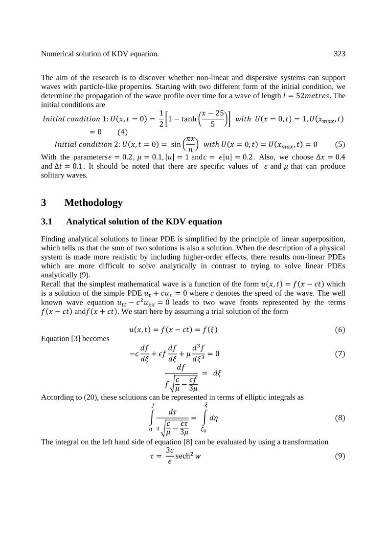
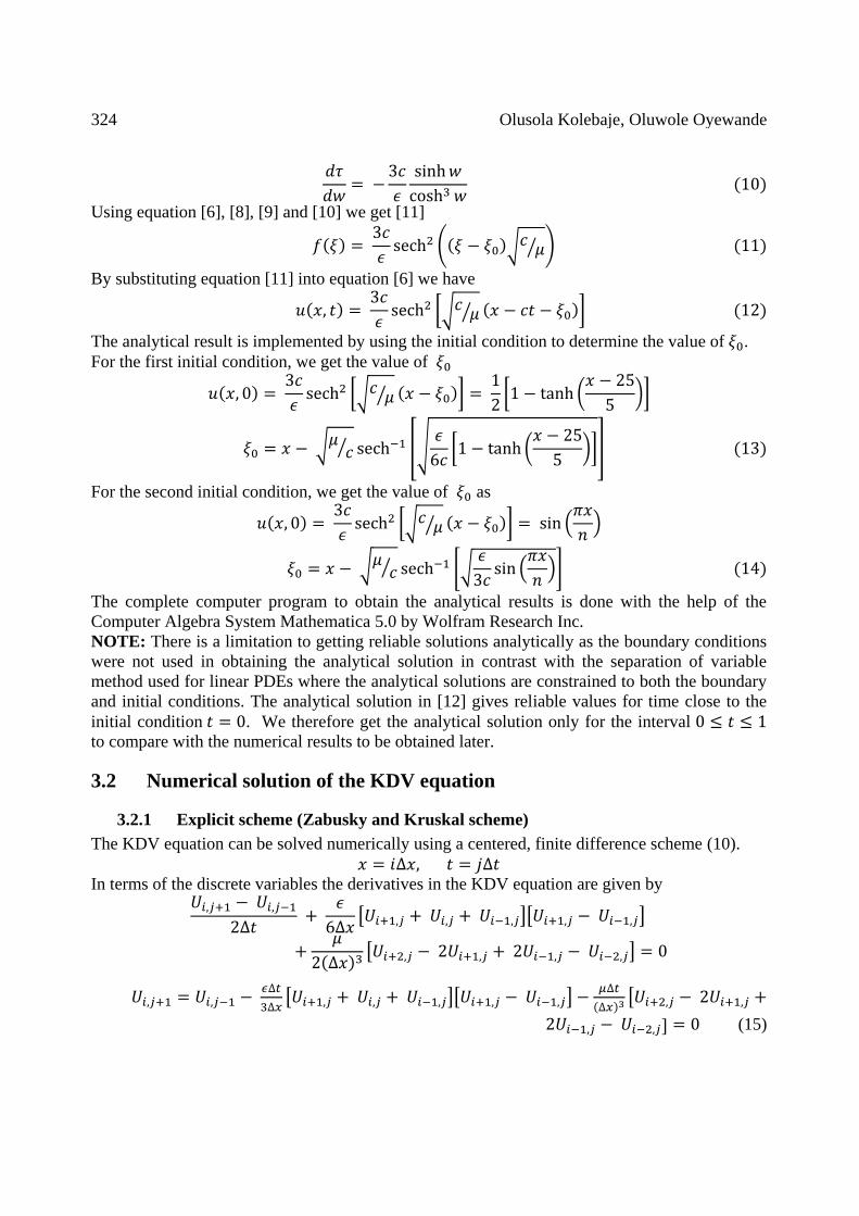
Fig 1 and Fig 2 show 3D graphical representation of the explicit scheme solution of the KDV

equation after 2000 time steps. The graphs were produced using MATLAB 7.8.0 from

Mathworks, Inc.

Figure 1: Explicit solution of the KDV equation (initial condition 1) after 2000 time steps (200

seconds).

Figure 2: Explicit solution of the KDV equation (initial condition 1) after 2000 time steps (200

seconds).

326 Olusola Kolebaje, Oluwole Oyewande

3.2.2 Implicit scheme (Goda scheme)

An implicit scheme for approximating the KDV equation was proposed by (21) and is extended

here to the KDV equation for all values of and .

Choosing , , and we

have a pentagonal system of linear equation to solve at each time step using LU decomposition

scheme for determining the inverse of a matrix.

(18)

The pentagonal system of linear equation can be written in matrix form as

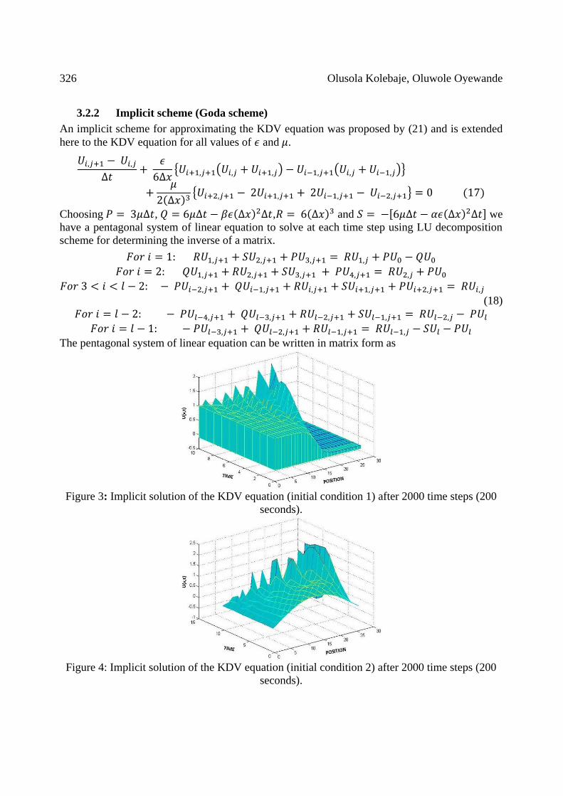
Figure 3: Implicit solution of the KDV equation (initial condition 1) after 2000 time steps (200

seconds).

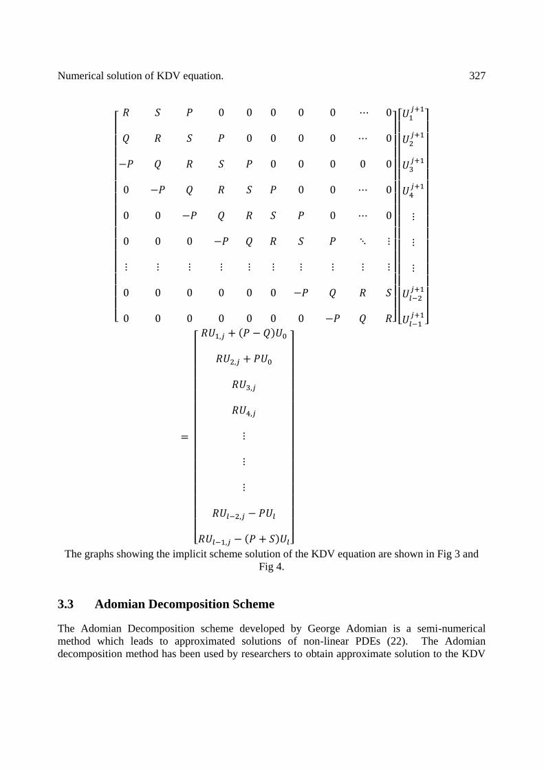
Figure 4: Implicit solution of the KDV equation (initial condition 2) after 2000 time steps (200

seconds).

Numerical solution of KDV equation. 327

The graphs showing the implicit scheme solution of the KDV equation are shown in Fig 3 and

Fig 4.

3.3 Adomian Decomposition Scheme

The Adomian Decomposition scheme developed by George Adomian is a semi-numerical

method which leads to approximated solutions of non-linear PDEs (22). The Adomian

decomposition method has been used by researchers to obtain approximate solution to the KDV

328 Olusola Kolebaje, Oluwole Oyewande

equation for different and values. (23) applied the Adomian decomposition for

and . (24) applied the method to the KDV equation with and . In

this work, we develop a formula for the KDV equation with any and values.

Recall the KDV equation in [3];

We define the operators

and so equation [3] can be written

in the form

From [19] we can write

We also define the inverse operator to operator given by

Applying the inverse operator in equation [21] on both sides of equation [20] gives

Where which is a constant of integration is the solution of the equation

and is just the

initial condition which is purely a function of .

The Adomian decomposition assumes that the solution to the PDE can be expressed by

an infinite series of the form

and the decomposed form of the non-linear operator into an infinite series of polynomials is

given by

are the Adomian special polynomials (22) and is an arbitrary parameter which aids in the

grouping of the terms. The parameterized form of equation [22] is written as

Comparing powers of gives

Numerical solution of KDV equation. 329

To obtain the Adomian polynomials we use equation [24]

(26)

Comparing powers of gives

If we approximate the values of the solution to the KDV equation using three terms, then we

have the solution

The computer program to determine the values of and the solution is

written in Mathematica 5.0 for initial condition 1 and 2 and the solutions are of the following

form:

For initial condition 1:

330 Olusola Kolebaje, Oluwole Oyewande

The three terms solution has 36 terms while the four terms solution has 92 terms.

For initial condition 2:

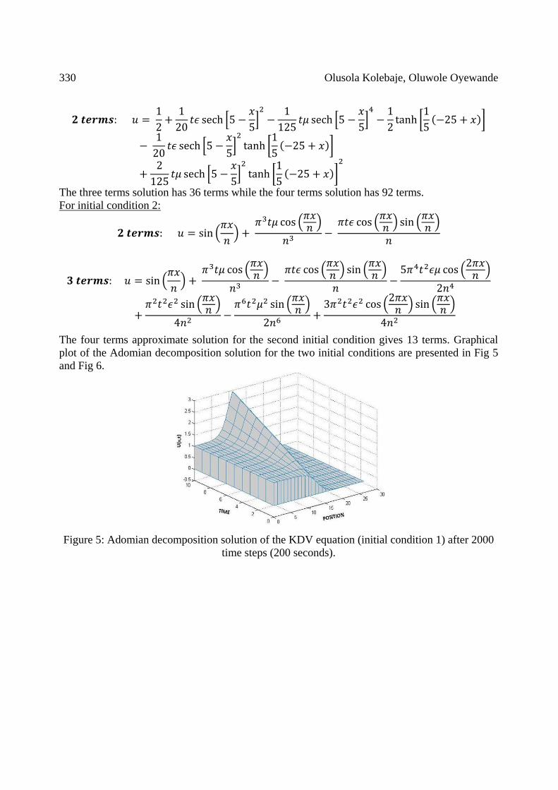
The four terms approximate solution for the second initial condition gives 13 terms. Graphical

plot of the Adomian decomposition solution for the two initial conditions are presented in Fig 5

and Fig 6.

Figure 5: Adomian decomposition solution of the KDV equation (initial condition 1) after 2000

time steps (200 seconds).

Numerical solution of KDV equation. 331

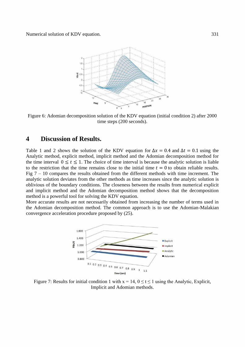
Figure 6: Adomian decomposition solution of the KDV equation (initial condition 2) after 2000

time steps (200 seconds).

4 Discussion of Results.

Table 1 and 2 shows the solution of the KDV equation for and using the

Analytic method, explicit method, implicit method and the Adomian decomposition method for

the time interval . The choice of time interval is because the analytic solution is liable

to the restriction that the time remains close to the initial time to obtain reliable results.

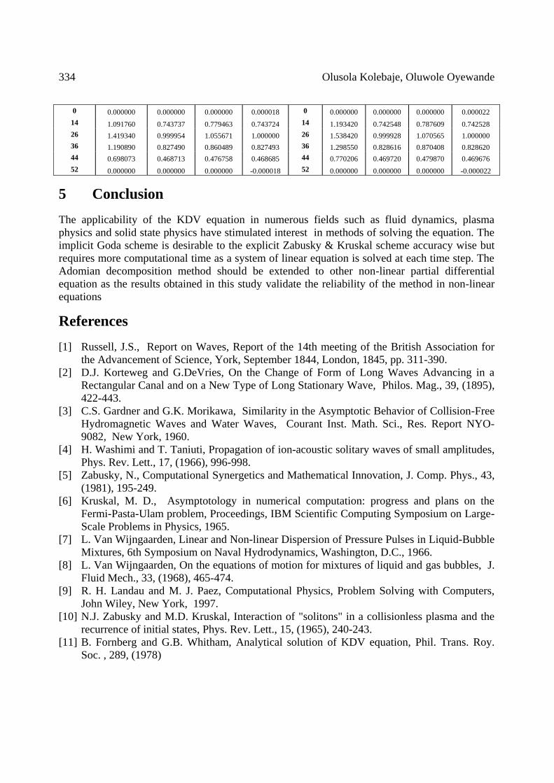
Fig 7 – 10 compares the results obtained from the different methods with time increment. The

analytic solution deviates from the other methods as time increases since the analytic solution is

oblivious of the boundary conditions. The closeness between the results from numerical explicit

and implicit method and the Adomian decomposition method shows that the decomposition

method is a powerful tool for solving the KDV equation.

More accurate results are not necessarily obtained from increasing the number of terms used in

the Adomian decomposition method. The common approach is to use the Adomian-Malakian

convergence acceleration procedure proposed by (25).

Figure 7: Results for initial condition 1 with x = 14, 0 ≤ t ≤ 1 using the Analytic, Explicit,

Implicit and Adomian methods.

332 Olusola Kolebaje, Oluwole Oyewande

Figure 8: Results for initial condition 1 with x = 44, 0 ≤ t ≤ 1 using the Analytic, Explicit,

Implicit and Adomian methods.

Figure 9: Results for initial condition 2 with x = 14, 0 ≤ t ≤ 1 using the Analytic, Explicit,

Implicit and Adomian methods.

Figure 10: Results for initial condition 2 with x = 44, 0 ≤ t ≤ 1 using the Analytic, Explicit,

Implicit and Adomian methods

Numerical solution of KDV equation. 333

Table 1: Results from initial condition 1 for and after 10 time steps for

comparison.

t = 0.0

x

Analytic Explicit Implicit Adomian

t = 0.2

x

Analytic Explicit Implicit Adomian

0 0.999955 0.999955 1.000000 0.999955 0 1.095520 1.000000 1.000000 0.999955

14 0.987872 0.987872 0.987872 0.987872 14 1.082600 0.988074 1.000961 0.988075

26 0.401312 0.401312 0.401312 0.401312 26 0.445677 0.402724 0.403922 0.402719

36 0.012128 0.012128 0.012128 0.012128 36 0.013578 0.012145 0.012116 0.012145

44 0.000500 0.000500 0.000500 0.000500 44 0.000560 0.000501 0.000499 0.000501

52 0.000020 0.000020 0.000000 0.000020 52 0.000023 0.000000 0.000000 0.000020

t = 0.4

x

Analytic Explicit Implicit Adomian

t = 0.6

x

Analytic Explicit Implicit Adomian

0 1.197420 1.000000 1.000000 0.999956 0 1.305460 1.000000 1.000000 0.999957

14 1.183680 0.988274 1.014401 0.988279 14 1.290920 0.988470 1.028206 0.988482

26 0.494476 0.404147 0.406569 0.404126 26 0.548039 0.405581 0.409255 0.405533

36 0.015200 0.012162 0.012104 0.012162 36 0.017016 0.012179 0.012092 0.012178

44 0.000627 0.000501 0.000499 0.000501 44 0.000702 0.000502 0.000498 0.000502

52 0.000026 0.000000 0.000000 0.000020 52 0.000029 0.000000 0.000000 0.000020

t = 0.8

x

Analytic Explicit Implicit Adomian

t = 1.0

x

Analytic Explicit Implicit Adomian

0 1.419280 1.000000 1.000000 0.999958 0 1.538360 1.000000 1.000000 0.999959

14 1.404010 0.988664 1.042389 0.988686 14 1.522440 0.988854 1.056967 0.988890

26 0.606693 0.407025 0.411981 0.406940 26 0.670756 0.408479 0.414748 0.408347

36 0.019048 0.012195 0.012080 0.012195 36 0.021321 0.012212 0.012067 0.012211

44 0.000786 0.000503 0.000497 0.000503 44 0.000881 0.000503 0.000497 0.000503

52 0.000032 0.000000 0.000000 0.000021 52 0.000036 0.000000 0.000000 0.000021

Table 2: Results from initial condition 2 for and after 10 time steps for

comparison.

t = 0.0

x

Analytic Explicit Implicit Adomian

t = 0.2

x

Analytic Explicit Implicit Adomian

0 0.000000 0.000000 0.000000 0.000000 0 0.000000 0.000000 0.000000 0.000004

14 0.748511 0.748511 0.748511 0.748511 14 0.824909 0.747315 0.756014 0.747314

26 1.000000 1.000000 1.000000 1.000000 26 1.095570 0.999997 1.013363 1.000000

36 0.822984 0.822984 0.822984 0.822984 36 0.905428 0.824111 0.832049 0.824111

44 0.464723 0.464723 0.464723 0.464723 44 0.515395 0.465715 0.467671 0.465714

52 0.000000 0.000000 0.000000 0.000000 52 0.000000 0.000000 0.000000 0.000004

t = 0.4

x

Analytic Explicit Implicit Adomian

t = 0.6

x

Analytic Explicit Implicit Adomian

0 0.000000 0.000000 0.000000 0.000009 0 0.000000 0.000000 0.000000 0.000013

14 0.907505 0.746121 0.763671 0.746118 14 0.996439 0.744928 0.771485 0.744921

26 1.197470 0.999988 1.027086 1.000000 26 1.305510 0.999974 1.041183 1.000000

36 0.994207 0.825237 0.841317 0.825238 36 1.089380 0.826364 0.850795 0.826366

44 0.570964 0.466711 0.470659 0.466704 44 0.631753 0.467710 0.473687 0.467695

52 0.000000 0.000000 0.000000 0.000009 52 0.000000 0.000000 0.000000 -0.000013

t = 0.8

x

Analytic Explicit Implicit Adomian

t = 1.0

x

Analytic Explicit Implicit Adomian

334 Olusola Kolebaje, Oluwole Oyewande

0 0.000000 0.000000 0.000000 0.000018 0 0.000000 0.000000 0.000000 0.000022

14 1.091760 0.743737 0.779463 0.743724 14 1.193420 0.742548 0.787609 0.742528

26 1.419340 0.999954 1.055671 1.000000 26 1.538420 0.999928 1.070565 1.000000

36 1.190890 0.827490 0.860489 0.827493 36 1.298550 0.828616 0.870408 0.828620

44 0.698073 0.468713 0.476758 0.468685 44 0.770206 0.469720 0.479870 0.469676

52 0.000000 0.000000 0.000000 -0.000018 52 0.000000 0.000000 0.000000 -0.000022

5 Conclusion

The applicability of the KDV equation in numerous fields such as fluid dynamics, plasma

physics and solid state physics have stimulated interest in methods of solving the equation. The

implicit Goda scheme is desirable to the explicit Zabusky & Kruskal scheme accuracy wise but

requires more computational time as a system of linear equation is solved at each time step. The

Adomian decomposition method should be extended to other non-linear partial differential

equation as the results obtained in this study validate the reliability of the method in non-linear

equations

References

[1] Russell, J.S., Report on Waves, Report of the 14th meeting of the British Association for

the Advancement of Science, York, September 1844, London, 1845, pp. 311-390.

[2] D.J. Korteweg and G.DeVries, On the Change of Form of Long Waves Advancing in a

Rectangular Canal and on a New Type of Long Stationary Wave, Philos. Mag., 39, (1895),

422-443.

[3] C.S. Gardner and G.K. Morikawa, Similarity in the Asymptotic Behavior of Collision-Free

Hydromagnetic Waves and Water Waves, Courant Inst. Math. Sci., Res. Report NYO-

9082, New York, 1960.

[4] H. Washimi and T. Taniuti, Propagation of ion-acoustic solitary waves of small amplitudes,

Phys. Rev. Lett., 17, (1966), 996-998.

[5] Zabusky, N., Computational Synergetics and Mathematical Innovation, J. Comp. Phys., 43,

(1981), 195-249.

[6] Kruskal, M. D., Asymptotology in numerical computation: progress and plans on the

Fermi-Pasta-Ulam problem, Proceedings, IBM Scientific Computing Symposium on Large-

Scale Problems in Physics, 1965.

[7] L. Van Wijngaarden, Linear and Non-linear Dispersion of Pressure Pulses in Liquid-Bubble

Mixtures, 6th Symposium on Naval Hydrodynamics, Washington, D.C., 1966.

[8] L. Van Wijngaarden, On the equations of motion for mixtures of liquid and gas bubbles, J.

Fluid Mech., 33, (1968), 465-474.

[9] R. H. Landau and M. J. Paez, Computational Physics, Problem Solving with Computers,

John Wiley, New York, 1997.

[10] N.J. Zabusky and M.D. Kruskal, Interaction of "solitons" in a collisionless plasma and the

recurrence of initial states, Phys. Rev. Lett., 15, (1965), 240-243.

[11] B. Fornberg and G.B. Whitham, Analytical solution of KDV equation, Phil. Trans. Roy.

Soc. , 289, (1978)

Numerical solution of KDV equation. 335

[12] Vvedenskii, D., Partial Differential Equations with Mathematica., Addison-Wesley,

Wokingham, 1992.

[13] Schiesser, W.E., Method of lines solution of the Korteweg de Vries equation, Comp. &

Maths. with Appls., 28, (1994), 147-154.

[14] Varley, E. and Seymour, B.R., A Simple Derivation of the N-Soliton Solutions to the

Korteweg de Vries Equation, SIAM Journal on Appl. Math., 58, (1998), 904-911.

[15] Barros, S. R. and Cardenas, J. W., A nonlinear Galerkin method for the shallow-water

equations on periodic domains, J. Comp. Phys., 172, (2002), 592-608.

[16] Ceniceros, H. D., A semi-implicit moving mesh method for the focusing nonlinear

Schrödinger equation, Comm. on Pure and Appl. Anals, 1, (2002), 1-14.

[17] Pasquetti, R., Spectral vanishing viscosity method for large-eddy simulation of turbulent

flows, Journal of Scientific Computing, (2006).

[18] Triki, H., Energy transfer in a dispersion-managed Korteweg-de Vries system, Mathematics

and Computer in Simulation. 2007.

[19] J. Aminuddin and Sehah, Numerical Solution of the Korteweg de Vries Equation,

International Journal of Basic & Applied Sciences, 11:2, (2011), 76-81.

[20] Drazin, P.G., Solitons, London Mathematical Society, Lecture Note Series 85, Cambridge

University Press, London, 1983.

[21] Goda, K., On instability of some finite difference schemes for the Korteweg-de Vries

equation J. Phys. Soc. Japan, 1 (1975).

[22] Adomian G., Solving Frontier Problems in Physics, The Decomposition Method, Kluwer

Academic Publishers, Boston, 1994.

[23] Ismail et al., Solitary wave solutions for the general KDV equation by Adomian

decomposition method, Applied Mathematics and Computation, Elsevier, 154 (2004), 17-

29.

[24] Mamaloukas, C., Numerical Solution of One Dimensional Korteweg de Vries Equation :

Geometry Balkan Press, 2001. Conference of Geometry and its Applications in Technology

and the Workshop on Global Analysis, Differential Geometry and Lie Algebras. pp. 121-

129.

[25] Rach R., A Convinient Computational Form of the Adomian Polynomials, J. Math. Anal.

Appl., 102 (1984).