NUMERICAL SOLUTION OF

STEADY-STATE ELECTRODIFFUSION

EQUATIONS FOR A SIMPLE MEMBRANE

RICHARD A. ARNDT, JAMES D. BOND, and L. DAVID ROPER

From the Department of Physics, Virginia Polytechnic Institute and State University, Blacks-burg, Virginia 24061

ABSTRACr A technique is given for obtaining numerical solutions to the steady-state electrodiffusion equations for a simple membrane. Solutions are given forseveral membrane boundary conditions in terms of ratios of current density to mo-bility for each ion type.

INTRODUCTION

Goldman (1943) solved the steady-state electrodiffusion equations for a simplemembrane (homogeneous and no charge structure) with either the assumption ofmicroscopic electroneutrality or of constant electric field. Bruner (1965 a, b; 1967)has numerically obtained solutions for special situations. He considered the solutionregions on each side of the membrane and applied boundary conditions at x = i oo

We report here a numerical method for obtaining solutions to the equations for asimple membrane for any boundary conditions at the membrane surfaces. We do notconsider the solutions on each side of the membrane because ion mobilities in manybiological membranes are -405 times smaller than mobilities in the surroundingsolutions (Cole, 1968). Later we shall alter this method for application to a dipole-layer membrane (Wei, 1969).Our method involves expanding the ion concentrations and the electric field in

Fourier series in the variable x (the position in the membrane). The series aretruncated and the coefficients are obtained by an iterative matrix technique.We give solutions for several membrane boundary conditions in terms of ratios

of current density to mobility for each ion type, and we compare results for differentvalues of the electric permittivity and membrane thickness. We find that the current-voltage curves for a biionic environment are essentially linear unless the concentra-tion gradients are large, but considerable deviation from nonlinearity can occur ina triionic environment if the ion mobilities are considerably different.

265

THEORY AND NUMERICAL PROCEDURE

The steady-state electrodiffusion equations are the Nernst-Planck and Poissonequations.

The Nernst-Planck Equation (Goldman, 1943)

dnk _1klk kk

dx ZkukRT (1)

where nk(X) is the concentration in moles per volume of ion type at position x,Zk is the valence, Uk is the mobility per unit valence (which we consider as constantacross the membrane), jk is the ion current density in the outward direction, E is theelectric field in the outward direction, and ,B = F/RT, where F is Faraday's constant,R is the universal gas constant, and T is the absolute temperature.

The Poisson Equation (Jackson, 1962).

dE F zknk (2)

where e is the permittivity (assumed constant across the membrane).Equation 1 can be converted to an integral equation by integrating both sides

from 0 to x:

nk(x) = nk - 7k X + Zk f f nk(x )E(x ) dx', (3)

where nk(i3 n,(O) is the ion concentration at the inside membrane boundary(x = 0). By evaluating equation 3 at the outside membrane boundary (x = w) weobtain an equation for the current density:

(k0 -n(o) Znk -nk + ZI nk(x)E(x ) dx, (4)

w wJ

where nk(o) nk(W) is the ion concentration at the outside boundary. Substitutionof equation 4 into equation 3 yields

nk(X) =iAk(X) + fk(x), (5)

where

n(o))nk(0)nkflk(x) =_nk + Xk

BIOPHYSIcAL JOURNAL VOLUME 11 1971266

and

fk(X) = Zk 3 [j nk(x')E(x') dx - -f nk(X)E(x) dx'],

which is the integral form of equation 1 and, in addition, contains the boundaryconditions at x = 0 and x = w. Note thatfk(O) = fk(w) = 0.We assume that electroneutrality holds at the membrane boundaries; i.e., that

E Zknk = 0 and E Zknk = 0. (6)k k

Perhaps some of these ions are essentially immobile in the membrane; that fact willcome in later when mobilities are explicitly considered.We shall solve numerically equations 5 and 2 simultaneously. In order to do so we

expand

L lirxfk(x) = (fk) sin- ,(7

i-i w

and

V L b7rxE(x) = - + El cos-, (8)w -i w

where the Fourier series are truncated at some value L to be determined empirically,and V is the electric potential at x = w relative to x = 0. The expansion functions,sin (hrx/w), in equation 7 vanish at x = 0 and x = w as does fk(x). The expansionfunctions, cos (lhx/w), in equation 8 are such that V = -f' Edx, which is thecorrect relation between E and V (Jackson, 1962).The expansion coefficients (fk) in equation 7 are obtained in the Appendix:

(fk) = (A,4k)im(yk)m ; (9)

the complicated expressions for (Yk)m and (Ak)ml are given in the Appendix (equa-tions A 1 and A 2). Equation 9 gives the ionic concentrations for a given input field,Ein, at some stage of the iteration. From thefk's the output field, Eout, as shown inthe Appendix (equation A 3), can be determined by

Emout Fw (10)eirm k

Now, incrementing the input field by an amount A will produce a change in the out-put field; we want to pick an increment A to change the input field to make it equalto the new output field. That is, we start with values for Em" , then calculate EmOut by

ARNDT ET AL. Solution ofSteady-State Electrodiffusion Equations 267

equations 9 and 10, and then solve for the vector A by means of the equations

Em + Am = Emout + ZEmEu A1, (11)

where OEmOUt/OE1in is obtained as indicated in the Appendix. This gives us a newinput field, Emin + A,, and we go through the procedure again.The numerical procedure is as follows:(a) Start with some electric field distribution (say, constant E) and calculate the

ion concentrations by equations 9, 7, and 5.(b) Calculate A by equation 11.(c) Change Ein by A and go back to step 1 until

X2= (Elin - Elout)2

is less than some small value.(d) Calculate Yk from equation 1.

TABLE I

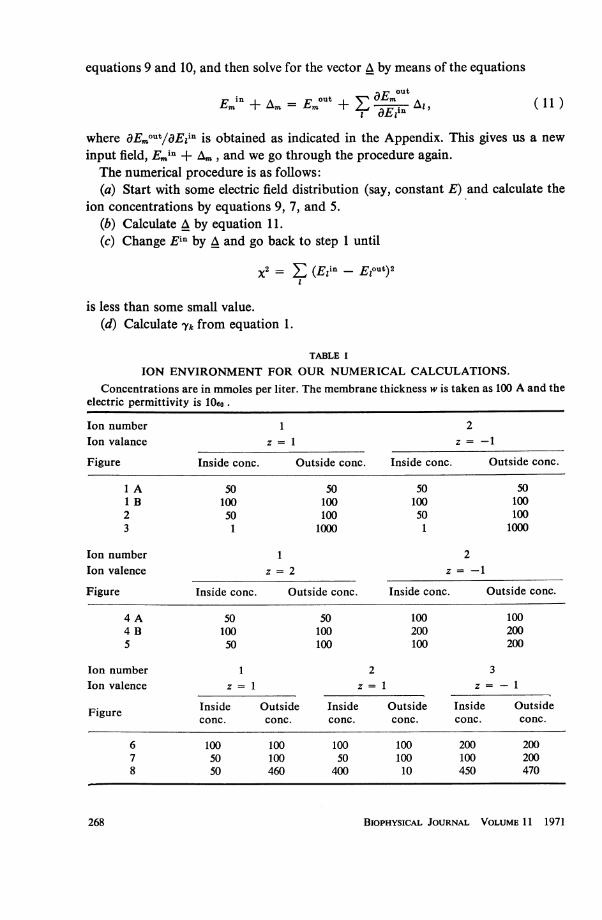
ION ENVIRONMENT FOR OUR NUMERICAL CALCULATIONS.Concentrations are in mmoles per liter. The membrane thickness w is taken as 100 A and the

electric permittivity is lOeo.

Ion number 1 2Ion valance z = 1 z = -1

Figure Inside conc. Outside conc. Inside conc. Outside conc.

1 A 50 50 50 501 B 100 100 100 1002 50 100 50 1003 1 1000 1 1000

Ion number 1 2Ion valence z =2 z -1

Figure Inside conc. Outside conc. Inside conc. Outside conc.

4 A 50 50 100 1004 B 100 100 200 2005 50 100 100 200

Ion number 1 2 3Ion valence z = 1 z = 1 z = -1

Inside Outside Inside Outside Inside OutsideFigure conc. conc. conc. conc. conc. conc.

6 100 100 100 100 200 2007 50 100 50 100 100 2008 50 460 400 10 450 470

BIOPHYSICAL JOURNAL VOLUME 11 1971268

APPLICATION

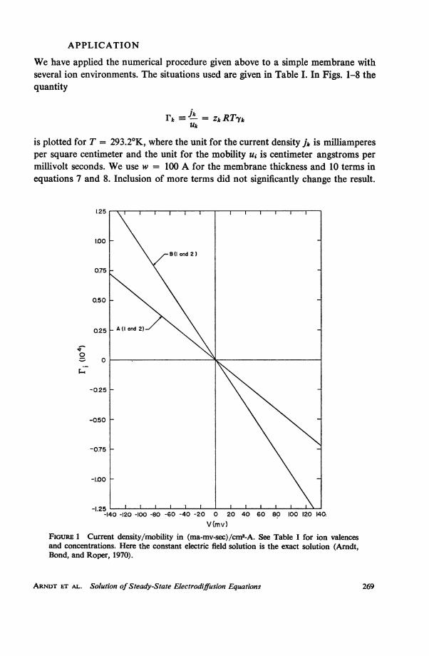
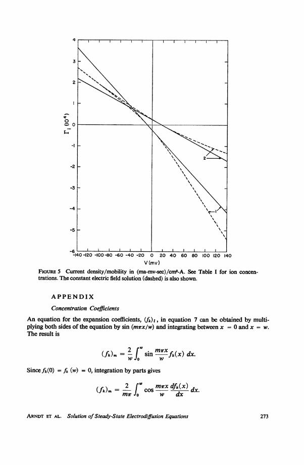
We have applied the numerical procedure given above to a simple membrane withseveral ion environments. The situations used are given in Table I. In Figs. 1-8 thequantity

rk - - = ZkRTYkUk

is plotted for T = 293.2°K, where the unit for the current density jk is milliamperesper square centimeter and the unit for the mobility ui is centimeter angstroms permillivolt seconds. We use w = 100 A for the membrane thickness and 10 terms inequations 7 and 8. Inclusion of more terms did not significantly change the result.

1.25 \ I

1.00

\B and 2)

0.75-

0.50

0.25 A(Ond 2)

0

-0.25 -

-0.50-

-075-

-1.25I .1-140 -120 -100 -80 -60 -40 -20 0 20 40 60 80 100 120 140

V(mv)FiGuRiE 1 Current density/mobility in (ma-mv-sec)/cm3-A. See Table I for ion valencesand concentrations. Here the constant electric field solution is the exact solution (Arndt,Bond, and Roper, 1970).

ARNDT ET AL. Solution ofSteady-State Electrodiffusion Equations 269

1.25

1.00

0.75

0.25

Q 0

-0.25

-0.50

-0.752

-1.00

-140 -120 -100 -80 -60 -40 -20 0 20 40 60 80 100 120 140

V (mv)

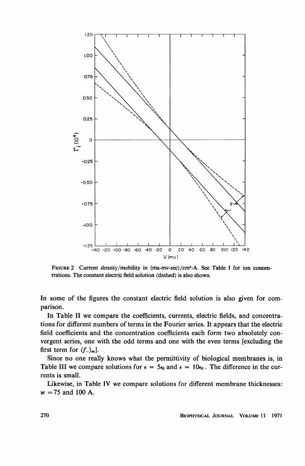
FiGuRE 2 Current density/mobility in (ma-mv-sec)/cm3-A. See Table I for ion concen-trations. The constant electric field solution (dashed) is also shown.

In some of the figures the constant electric field solution is also given for com-parison.

In Table II we compare the coefficients, currents, electric fields, and concentra-tions for different numbers of terms in the Fourier series. It appears that the electricfield coefficients and the concentration coefficients each form two absolutely con-vergent series, one with the odd terms and one with the even terms [excluding thefirst term for (f-)m].

Since no one really knows what the permittivity of biological membranes is, inTable III we compare solutions for e = 5eo and e = lOEo . The difference in the cur-rents is small.

Likewise, in Table IV we compare solutions for different membrane thicknesses:w =75 and 100 A.

BIOPHYSICAL JOURNAL VOLUME 11 1971270

5

4

3

2

00

-:4

-5-140 -120 -100 -80 -60 -40 -20 o 20 40 60 80 100 120 140

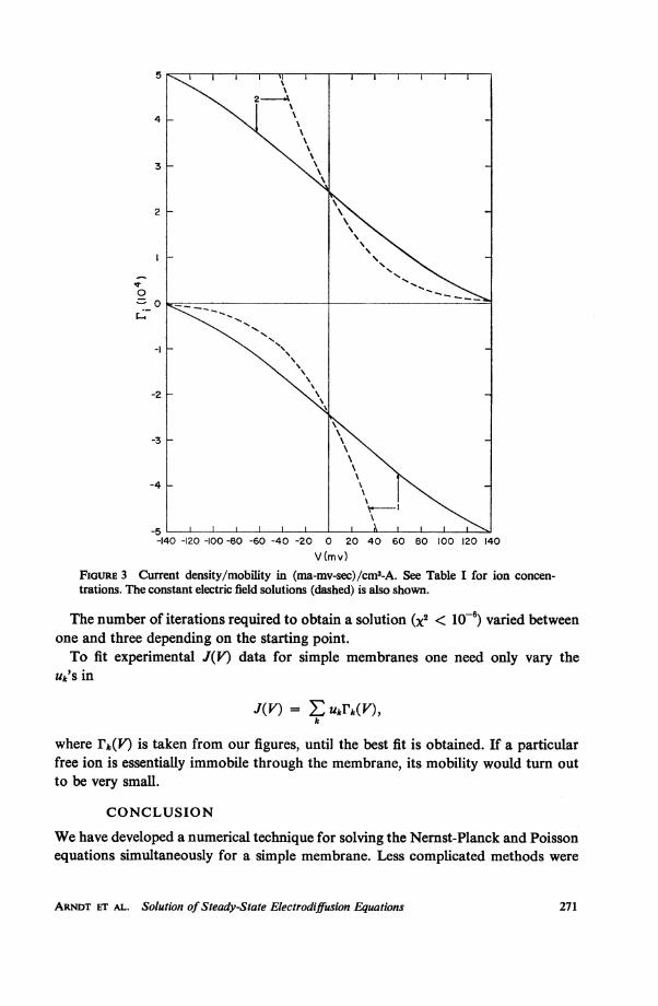
V (mv)FIGURE 3 Current density/mobility in (ma-mv-sec)/cm3-A. See Table I for ion concen-trations. The constant electric field solutions (dashed) is also shown.

The number of iterations required to obtain a solutionl (XI < 10-') varied betweenone and three depending on the starting point.To fit experimental J(V) data for simple membranes one need only vary the

Ukis in

J(V) =EUkrk(V),

k

where rk(v) is taken from our figures, until the best fit is obtained. If a particularfree ion is essentially immobile through the membrane, its mobility would turn outto be very small.

CONCLUSION

We have developed a numerical technique for solving the Nernst-Planck and Poissonequations simultaneously for a simple membrane. Less complicated methods were

ARNDT ET AL. Solution ofSteady-State Electrodiffusion Equations 271

5

4

3 B

2 2

-2

-3

-4

-140-120 -100 -80 -60 -40 -20 0 20 40 60 80 100 120 140

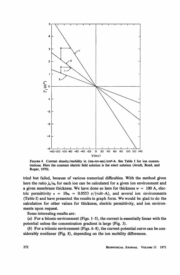
V(mv)FiGuRE 4 Current density/mobility in (ma-mv-sec)/cm3-A. See Table I for ion concen-trations. Here the constant electric field solution is the exact solution (Arndt, Bond, andRoper, 1970).

tried but failed, because of various numerical difficulties. With the method givenhere the ratio jk/uk for each ion can be calculated for a given ion environment anda given membrane thickness. We have done so here for thickness w = 100 A, elec-tric permittivity e = lOeo = 0.0553 e/(volt-A), and several ion environments(Table I) and have presented the results in graph form. We would be glad to do thecalculation for other values for thickness, electric permittivity, and ion environ-ments upon request.Some interesting results are:(a) For a biionic environment (Figs. 1-5), the current is essentially linear with the

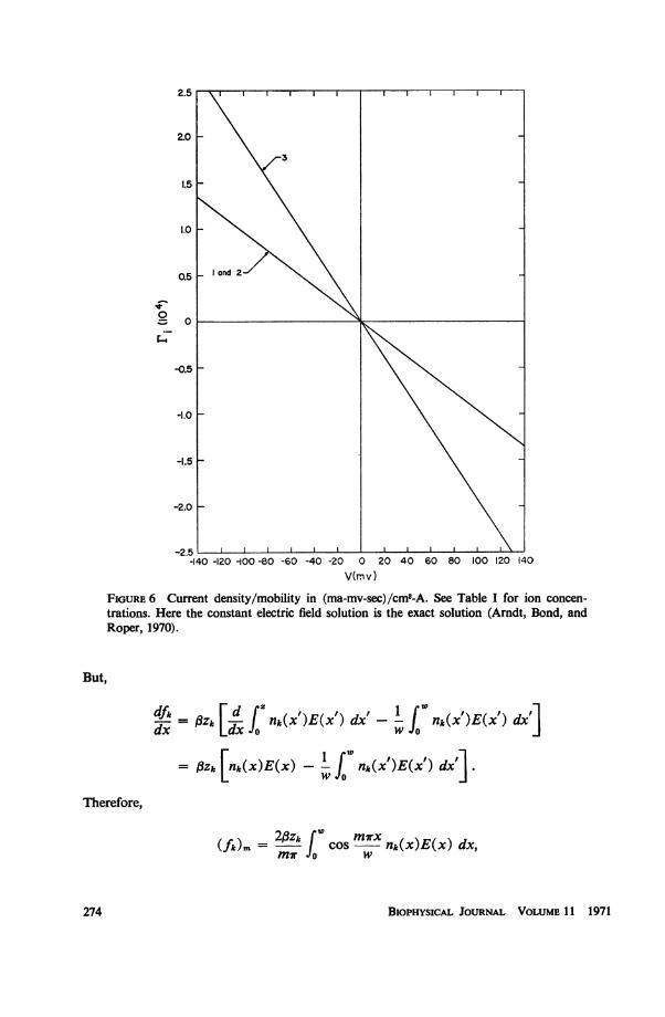
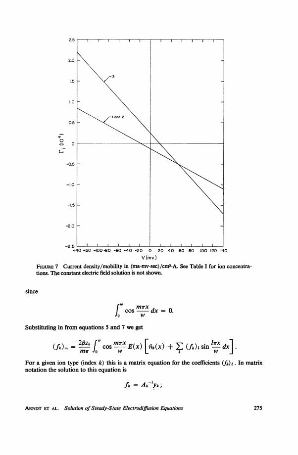
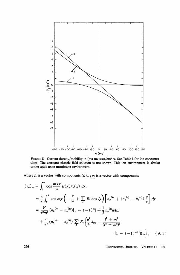
potential unless the concentration gradient is large (Fig. 3).(b) For a triionic environment (Figs. 6-8), the current-potential curve can be con-

siderably nonlinear (Fig. 8), depending on the ion mobility differences.

BIOPHYSICAL JOURNAL VOLUME 11 1971272

4

0

-2

-3

-4

-5

-6-140 -120 -100 -80 -60 -40 -20 0 20 40 60 80 100 120 140

V(mv)FIGuRE 5 Current density/mobility in (ma-mv-sec)/cm3-A. See Table I for ion concen-trations. The constant electric field solution (dashed) is also shown.

APPENDIX

Concentration Coefficients

An equation for the expansion coefficients, (l)1, in equation 7 can be obtained by multi-plying both sides of the equation by sin (mTx/w) and integrating between x = 0 and x = w.The result is

(fk)m= 2 f sin mTXfk(x) dx.

Since fk(O) = fk (w) = 0, integration by parts gives

(fk)m = cos =x dx.M7r o w dx

ARNDT ET AL. Solution ofSteady-State Electrodiffusion Equations 273

0

-0.5

-1.0

-1.5

-2.0

-2.5 , t X-140 -120 -100 -80 -60 -40 -20 0 20 40 60 80 100 120 140

V(rnv)

FIGURE 6 Current density/mobility in (ma-mv-sec)/cm8-A. See Table I for ion concen-trations. Here the constant electric field solution is the exact solution (Arndt, Bond, andRoper, 1970).

But,

= #Zk nk(x')E(x') dx'-1 JWnk(x')E(x) dx']

= JZk [nk(x)E(x) - !| nk(x')E(x') dx']

Therefore,

(fk)m = | cos nk(x)E(x) dx,mir J W

BIoPHYSICAL JOURNAL VOLUME 11 1971274

2.5

2.0-

-.5

1.0

0.5-

0

-0.5-

-1.0

-i.5

-2.0

-140 -120 -100-80 -60 -40 -20 0 20 40 60 80 100 120 140V (mv)

FIGuRE 7 Current density/mobility in (ma-mv-sec)/cm3-A. See Table I for ion concentra-tions. The constant electric field solution is not shown.

since

f mirxdxOlwcos mxdx= 0

ow

Substituting in from equations 5 and 7 we get

(OM = 2zk cos m7x E(x) At(x) + Ei(fit) sin l- dx -MrrJ w

For a given ion type (index k) this is a matrix equation for the coefficients (fI) I. In matrixnotation the solution to this equation is

fi A= -

ARNDT ET AL. Solution of Steady-State Electrodiffusion Equations 275

6

5 3

4

3

-2

-3

-4

-5

-6

-7

-140 -120 -100 -80 -60 -40 -20 0 20 40 60 80 100 120 140

V (mv)FIGURE 8 Current density/mobility in (ma-mv-sec)/cm3-A. See Table I for ion concentra-tions. The constant electric field solution is not shown. This ion environment is similarto the squid axon membrane environment.

wherefk is a vector with components (Jk)m; Yk is a vector with components

(Yk)m Cos mrx E(x)flk(x) dx,

=-h f cos my - + Z El cos ly) [nk + (nk - nk ) -] dyir 0 W rj

V (f(o) - .W\i 1m=rm(nk °)nk()[_ (l)mn] + nk)wEn

- r2M2 IkL ' 2

+ 2 (nk(o) -nk()) El fir2^1_ -2+ m2

- (-1)m+l]im}, (A1)

BIOPHYSICAL JOURNAL VOLUME 11 1971276

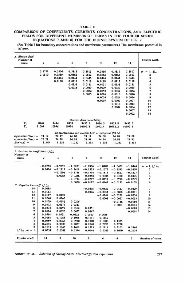
TABLE II

COMPARISON OF COEFFICIENTS, CURRENTS, CONCENTRATIONS, AND ELECTRICFIELDS FOR DIFFERENT NUMBERS OF TERMS IN THE FOURIER SERIES

(EQUATIONS 7 AND 8) FOR THE BIIONIC SYSTEM OF FIG. 2.(See Table I for boundary concentrations and membrane parameters.) The membrane potential is

-140 mv.

A. Electric fieldNumber of Fourier coeff.terms 2 4 6 8 10 12 14

0.3779 0.3806 0.3813 0.3815 0.3816 0.3817 0.3817 m = 1, Em0.0510 0.0559 0.0562 0.0562 0.0562 0.0563 0.0563 2

0.0444 0.0444 0.0445 0.0444 0.0444 0.0444 30.0108 0.0118 0.0118 0.0118 0.0118 0.0118 4

0.0131 0.0131 0.0131 0.0131 0.0131 50.0036 0.0039 0.0039 0.0039 0.0039 6

0.0052 0.0052 0.0052 0.0052 70.0015 0.0016 0.0016 0.0016 8

0.0024 0.0024 0.0024 90.0007 0.0007 0.0007 10

0.0013 0.0013 110.0004 0.0004 12

0.0007 130.0002 14

Current density/mobilityr+ 8469 8444 8438 8435.5 8434.5 8433.8 8433.5r_. 11007 10996 10994 10992.8 10992.4 10992.2 10992.1

Concentrations and electric field at midpoint (50 A)n4(mmoles/liter) = 74.12 74.17 74.08 74.11 74.08 74.09 74.08n/(mmoles/liter) = 75.21 74.88 74.98 74.91 74.94 74.91 74.93E(mv/A) = 1.349 1.355 1.352 1.353 1.353 1.353 1.353

B. Positive ion coefficients (f+)mNumber ofterms 2 4 6 8 10 12 14 Fourier Coeff.

-0.8752 -0.9896 -1.0223 -1.0336 -1.0402 -1.0429 -1.0444 m = 1, (f+),n0.0404 -0.1117 -0.1418 -0.1525 -0.1572 -0.1595 -0.1609 2

-0.1596 -0.1748 -0.1794 -0.1813 -0.1822 -0.1827 30.0084 -0.0286 -0.0358 -0.0386 -0.0398 -0.0405 4

-0.0734 -0.0777 -0.0791 -0.0796 -0.0799 50.0020 -0.0117 -0.0143 -0.0153 -0.0159 6

C. Negative ion coeff. (f-)m14 0.0085 -0.0405 -0.0422 -0.0427 -0.0429 713 0.0163 0.0006 -0.0054 -0.0066 -0.0071 812 0.0117 0.0129 -0.0244 -0.0251 -0.0254 911 0.0240 0.0245 0.0003 -0.0027 -0.0033 1010 0.0179 0.0186 0.0206 -0.0156 -0.0160 119 0.0373 0.0377 0.0387 0.0001 -0.0015 128 0.0293 0.0299 0.0312 0.0351 -0.0105 137 0.0616 0.0620 0.0627 0.0647 0.0001 146 0.0514 0.0521 0.0532 0.0560 0.06485 0.1084 0.1088 0.1095 0.1111 0.11574 0.0959 0.0966 0.0980 0.1008 0.1080 0.13353 0.2015 0.2020 0.2029 0.2048 0.2093 0.22382 0.1633 0.1645 0.1669 0.1715 0.1819 0.2105 0.3340

(ff)" m = 1 0.0554 0.0568 0.0594 0.0646 0.0763 0.1070 0.2134

Fourier coeff. 14 12 10 8 6 4 2 Number of terms

ARNDT ET AL. Solution of Steady-State Electrodiffusion Equations 277

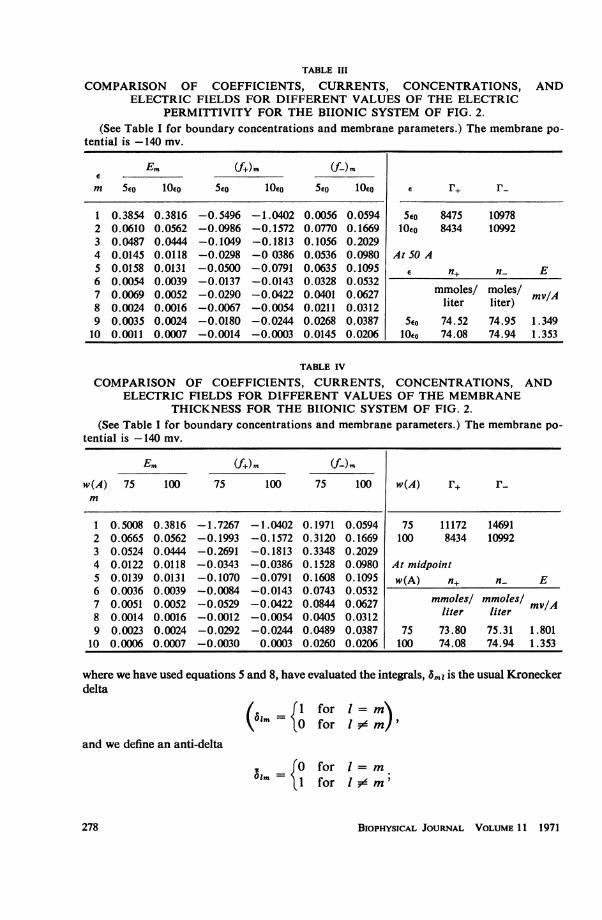
TABLE III

COMPARISON OF COEFFICIENTS, CURRENTS, CONCENTRATIONS, ANDELECTRIC FIELDS FOR DIFFERENT VALUES OF THE ELECTRIC

PERMITTIVITY FOR THE BIIONIC SYSTEM OF FIG. 2.(See Table I for boundary concentrations and membrane parameters.) The membrane po-

tential is -140 mV.

Em (f+)m (fi-)me -

m 5eo lOeo 5eo lOeo 5eo 10or e +

1 0.3854 0.3816 -0.5496 -1.0402 0.0056 0.0594 5eo 8475 109782 0.0610 0.0562 -0.0986 -0.1572 0.0770 0.1669 1OEo 8434 109923 0.0487 0.0444 -0.1049 -0.1813 0.1056 0.20294 0.0145 0.0118 -0.0298 -0 0386 0.0536 0.0980 At 50 A5 0.0158 0.0131 -0.0500 -0.0791 0.0635 0.1095 e n+ n_ E6 0.0054 0.0039 -0.0137 -0.0143 0.0328 0.0532 mmoles/ moles/7 0.0069 0.0052 -0.0290 -0.0422 0.0401 0.0627 ler ler) mvIA8 0.0024 0.0016 -0.0067 -0.0054 0.0211 0.0312 liter liter)9 0.0035 0.0024 -0.0180 -0.0244 0.0268 0.0387 5eo 74.52 74.95 1.34910 0.0011 0.0007 -0.0014 -0.0003 0.0145 0.0206 lOeo 74.08 74.94 1.353

TABLE IV

COMPARISON OF COEFFICIENTS, CURRENTS, CONCENTRATIONS, ANDELECTRIC FIELDS FOR DIFFERENT VALUES OF THE MEMBRANE

THICKNESS FOR THE BIIONIC SYSTEM OF FIG. 2.(See Table I for boundary concentrations and membrane parameters.) The membrane po-

tential is -140 mv.

Em .f+)r (f-)m

w(A) 75 100 75 100 75 100 w(A) r+ .m

1 0.5008 0.3816 -1.7267 -1.0402 0.1971 0.0594 75 11172 146912 0.0665 0.0562 -0.1993 -0.1572 0.3120 0.1669 100 8434 109923 0.0524 0.0444 -0.2691 -0.1813 0.3348 0.20294 0.0122 0.0118 -0.0343 -0.0386 0.1528 0.0980 At midpoint5 0.0139 0.0131 -0.1070 -0.0791 0.1608 0.1095 w(A) n+ n_ E6 0.0036 0.0039 -0.0084 -0.0143 0.0743 0.05327 0.0051 0.0052 -0.0529 -0.0422 0.0844 0.0627 mmoles/ mmoles/ mv/A8 0.0014 0.0016 -0.0012 -0.0054 0.0405 0.0312 liter liter9 0.0023 0.0024 -0.0292 -0.0244 0.0489 0.0387 75 73.80 75.31 1.801

10 0.0006 0.0007 -0.0030 0.0003 0.0260 0.0206 100 74.08 74.94 1.353

where we have used equations 5 and 8, have evaluated the integrals, 5,mI is the usual Kroneckerdelta

i=I for l= m\0 for I m/m

and we define an anti-delta

Si.fO for l= mLm~ lI for l

5 m'

BIOPHYSICAL JOURNAL VOLUME 11 1971278

and Ak is a matrix with elements

mir w mTrx Irx(Ak)ml c2os 8m1 JOsin - E(x) dx

mTr w FT=5mi-- | cos my sin Iy (-- + Er cs ry) dy-2I3zk Jow

2-zk + 7r(12 V m2) [1 -

1w 2 2 r2--E Er [12 - (m + r)2[12 -(m - r)2] [1 ( 1) ]. (A 2)

Of course, one needs the Em coefficients to obtain fk.

Electric Field CoefficientsPoisson's equation, equation 2, and equation 8 combine to give

F it . Irx-Z Zknk(X) = -- IE sin-.E k W I W

But, according to equation 5

ZZk fk(X) = ( [f (x')E(x') dx' - f- q(x')E(x') dx'] = Z Zkfk(X),

where n (x) =- k zk2nk(X), because

E Zk lk(X) = ZZkkknk - Zknk =0

by equation 6. Therefore,

ZEI,sin liO ,w fEdx-xfwE dxlI w O[r LJ w J0 J

The expansion coefficients, El, can be obtained by multiplying both sides of this equation bysin (m7rx/w) and integrating between x = 0 and x = w. Then

wE F(w [mE mrx fn(x')E(x') dx' dx2 ~ L0 w 0

--1 fr(x')E(x') dx' x sin mrx dx]w oo w

F3w [t q(x')E(x') sin mx dx dx'w

+-(O,Wwf o(x')E(x') dx']

ARNDT ET AL. Solution of Steady-State Electrodiffusion Equations 279

where we have used

rw r2 w w

ffj g(x', x) dx' dx = f g(x', x) dx dx',

a standard relation for an arbitrary integrand g(x', x) in the first double integral and an in-tegral table (or integration by parts) in the second double integral. The integral involvingsin (m7rx/w) can be evaluated to give

Em = 2Fw f cos mrx (x)E(x) dx.

Now substitute equation 8 for E(x):

m2r2e V w mirx fW MrX lxEm = J0 cos 77(x) dx-L El cos cos n(x) dx.2F,Bw w Jo w z o w x

This equation can be considered as an equation for obtaining an output electric field, repre-sented by Em°ut for some given input field, represented by El . [Note that 0 (x) is a functionof Elin.] We use the numerical method of finite differencing to find ,Emout/aE1in from thisequation.

Poisson's equation can also be formulated as

F F F h7rX b7rx-E Zknk(x) =- Zkfk(X)=- ZkE(fk) Isin = EZ IEzsin-,E k f k e k I W WI W

or

Eo~ut =-Fw ( 3Emot= E Zk(fk)m)f ( A 3)firM k

where the (fk)m are obtained from an input field, Ein, by equation (A 1).

Received for publication 14 Jiuly 1970 and in revisedform 16 September 1970.

REFERENCES

ARNDT, R. A., J. D. BoND, and L. D. ROPER. 1970. Biophys. J. 10:1149.BRUNER, L. J. 1965 a. Biophys. J. 5:867.BRUNER, L. J. 1965 b. Biophys. J. 5:887.BRUNER, L. J. 1967. Biophys. J. 7:947.COLE, K. S. 1968. Membranes, Ions and Impulses. University of California Press, Berkeley. 186.GOLDMAN, D. E. 1943. J. Gen. Physiol. 27:37.JACKSON, J. D. 1962. Classical Electrodynamics. John Wiley and Sons, Inc., New York. 12, 133.WEI, L. Y. 1969. Bull. Math. Biophys. 31:39.

280 BIOPHYSICAL JOURNAL VOLUME 11 1971