Numerical solution of eigenvalue problems in acoustic field

Numerical solution of eigenvalueproblems in acoustic field

computation and car design

Volker MehrmannMATHEON, TU Berlin, Institut für Mathematik

DFG Research Center MATHEONMathematics for key technologies

Novi Sad 12.06.12

Outline

1 Introduction2 Adaptive Finite Elements3 Adaptivity and homotopy

Interior Car Acoustics 2 / 59

Optimality through mathematics

. Society is increasingly sensitive to inconveniences that comewith modern technologies such as air and water pollution,noise by airplanes, cars, trains.

. There is an increasing demand for optimal solutions. Minimalenergy consumption, minimal noise, pollution, waste.

. Optimal solutions need mathematical techniques, such asmodel based optimization/control.

. We need better mathematical models, faster and moreaccurate numerical methods, robust implementations onmodern computer architectures.

. The progress through better methods exceeds theprogress through better hardware by large factors.


Common attitude

. Our industry has built cars, trains airplanes for ages.

. Most engineers get away with the math from the first year.

. For the solution of differential equations, eigenvalue problems,optimization problems, etc., there are wonderful commercialpackages? They always deliver good solutions.

. If the problems become more complex then we just buy abigger computer.

. We don’t really need mathematics except maybe aslanguage for describing the models.

. Optimization? We just use genetic algorithms, they alwaysfind the optimal solution.


Anti-theses

No key technology development without modernmathematical technology!We need:

. Very good mathematical models, that represent thetechnological process well.

. Deep understanding of the models and the dynamics of theprocesses.

. Accurate and efficient algorithms to simulate themodels/processes.

. Accurate and efficient methods to control and optimize theprocesses and products.


An industrial example

Acoustic field optimization: Industrial Project with SFE in Berlin.→ film

. Model for acoustic field within a car.

. SFE has its own parameterized FEM model which allowssimple geometry and topology changes.

. Goal: Minimize noise in important regions inside the car usingchanges in geometry, topology, damping material, etc.

. Discretized model has up to size 10,000,000 or bigger.

. Model order reduction to reduce size of model for optimization.


Acoustic Field Optimization

SFE GmbH, BerlinCEO: Hans [email protected]://www.sfe-berlin.de

© SFE GmbH 2007

SFE AKUSMOD

DLOAD 1 = symmetrical excitationDLOAD 2 = antimetrical excitation

Unit force = 1 N mm

grid-ID 31010

grid-ID 31011


Optimization and discretization

. For SFE, discretization means modeling with discrete model.

. For costumers of SFE, Optimization means playing with theparameter until a certain acoustic field is achieved.

. A reduced order model is needed for small response timesand optimization.

. One determines the important modes by solving nonlineareigenvalue problems.

. Can this be automatized by prescribing a cost functional andreally doing optimization?

. Is the fine discretization that is used in the ’forward PDE’ reallya good discretization if we then afterwards have to use modelreduction to throw away all the unimportant staff.


Mathematical BackgroundThe 3-D lossless wave equation (in air) is derived from:1. The continuity equation (conservation of mass):

∂ρ

∂t+∇(ρv) = 0.

2. The Euler equation (Newton’s Second Law)

ρ(∂v∂t

+ (v · ∇)v) = −∇p

v = v(x ; y ; z; t) particle velocity,ρ = ρ(x ; y ; z; t) particle density,p = p(x ; y ; z; t) pressure.


Simplifications

Assumptions:. There is no temperature change.. The fluid is inviscid (no shear forces).. No influence of external forces.. We can make the expansions

p = p0 + p(x ; y ; z; t) with p0 p (p0 = 106p),

ρ = ρ0 + ρ(x ; y ; z; t) with ρ0 ρ.

. Adiabatic fluid (no heat exchange during compression).

. Ideal gas ρ = pc2 where c is the speed of sound.

. (v · ∇)v and ρ∂v∂t are small.


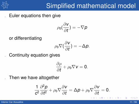
Simplified mathematical model. Euler equations then give

ρ0(∂v∂t

) = −∇p

or differentiating

ρ0∇(∂v∂t

) = −∆p.

. Continuity equation gives

∂ρ

∂t+ ρ0∇v = 0.

. Then we have altogether

1c2

∂2p∂t2 + ρ0∇

∂v∂t

= ∆p + ρ0∇∂v∂t

= 0.


Fluid structure interaction

The fluid-structure interaction is modeled via boundaryconditions.

Let u be the displacement of the car body on the surface. Thenv = ∂u

∂t and thus with the outer normal ν we get

νρ0∂2u∂t2 = −ν∇p.


Variational formulation

Multiply with a test function w , using integration by parts byintegrating over control volumes V with surface elements S:∫

V

1c2 w

∂2

∂t2 p dV +

∫V

(∇w)∇p dV = −ρ0

∫Sνw

∂2u∂t2 dS,

or equivalently∫V

1ρ0c2 w

∂2

∂t2 dV +

∫V

1ρ0

(∇w)∇p dV = −∫

Sνw

∂2u∂t2 dS.


Absorbing surface

Damping/absorption is realized by the additional term:∫S

wr

ρ20c2

∂p∂t

dS,

where r is a material dependent parameter r = r(α). Thus:∫V

1ρ0c2 w

∂2

∂t2 p dV +

∫V

1ρ0

(∇w)∇pdV

+

∫S

wr

ρ20c2

∂p∂t

dS = −∫

Sνw

∂2ut2 dS.


Finite element model: fluid

Discretization via FE shape functions in space yields thediscretized second order system

Mf pd + Df pd + Kf pd + Dsf ud = 0.

Here Mf = MTf and Kf = K T

f are positive definite and Df issymmetric positive semidefinite, Dsf describes the coupling.


Finite element model: structure

The (discrete) finite element model for the vibration of thestructure (linear materials) is:

Msud + Dsud + Ksud = fe + fp.

Here fe is a (discrete) external load and fp is the pressure load.Ms,Ds,Ks are real symm. pos. semidef. mass/damping/stiffnessmatrices of the structure. Ms is singular and diagonal.


Fluid structure coupling

The term fp originates from the pressure load Fp =∫

S pν dS.This yields fp = DT

sf pd and hence

Msud + Dsud + Ksud − DTsf pd = fe.

Here the stiffness matrix Ks = K1(ω) + ıK2 is complex symmetricand frequency dependent.


Full model: summary

[Ms 0DT

sf Mf

] [ud

pd

]+

[Ds 00 Df

] [ud

pd

]+

[Ks(ω) Dsf

0 Kf

] [ud

pd

]=

[fs0

].

. Ms,Mf ,Kf are real symm. pos. semidef. mass/stiffnessmatrices of structure and air, Ms is singular and diagonal, Ms

is a factor 1000− 10000 larger than Mf .. Ks(ω) = Ks(ω)T = K1(ω) + ıK2.. Ds,Df are real symmetric damping matrices.. Dsf is real coupling matrix between structure and air.. Parts depend on geometry, topology and material parameters.


Reformulation of evp

(λ2[

Ms 0DT

sf Mf

]+ λ

[Ds 00 Df

]+

[Ks(ω) Dsf

0 Kf

])[xs

xf

]= 0,

or after scaling second block row with λ−1 and second blockcolumn with λ one has the complex symmetric quadratic evp(λ2[

Ms 00 Mf

]+ λ

[Ds Dsf

DTsf Df

]+

[Ks(ω) 0

0 Kf

])[xs

λ−1xf

]= 0.


Numerical methods for nonlinear evpsMethods directly for nonlinear problems (incomplete list). Forrecent surveys see M./Voss 2005 or Dissertation Schreiber2008.. Second order Arnoldi method Bai 2006. Rational Krylov method Ruhe 1998, 2000. Residual iteration method Neumaier 1985. Newton-Type methods Schreiber/Schwetlick 2006, 2008,. Rayleigh quotient iterations Schreiber 2008, Freitag/Spence

2007, 2008. Jacobi-Davidson methods Sleijpen/Van der Vorst et al 1996,

Betcke/Voss 2004, Hochstenbach 2007. Arnoldi type methods Voss 2003. Eigenvalue continuation Beyn/Tümmler 2005,2008


Can we use these methods?

. None of these methods can be applied directly.

. Previous decoupled methods for structure/fluid subsystemsdo not work appropriately.

. One cannot guarantee that all desired ev’s are obtained and agiven relative residual?

. Evp is truely nonlinear.

. Problem is very ill-conditioned or even singular for someparameter sets.

. Mass matrix is block diagonal, but singular.

. The methods have to run as parallel methods on modernmulti-core machines.


Nonlinear Newton evp. solver.Truely nonlinear evp P(λ)x = (λ2M + λD + K (λ))x = 0.Apply Newton to function

fw (x , λ) =

[P(λ)x

wHx − 1

]= 0.

The Newton system for λk+1 = λk + µk and xk+1 = xk + sk is[P(λk ) P(λk )xk

wH 0

] [sk

µk

]= −

[P(λk )xk

wHxk − 1

]or

λk+1 = λk −1

wHP(λk )−1P(λk )xk

xk+1 = (λk − λk+1)P(λk )−1P(λk )xk .


Difficulties

. We want many eigenvalues 50− 100.

. Need to use out-of-core sparse solvers for shift-and-invert.

. Need to get into convergence intervals for Newton,Jacobi-Davidson.

. We really need nonlinear model reduction (open problem).

. We need to use the fact that only a small part of the system ischanged in every optimization step.

. We need to integrate ev computation, gradient computation,discretization.

. Adaptive multilevel FEM for evs would be great.


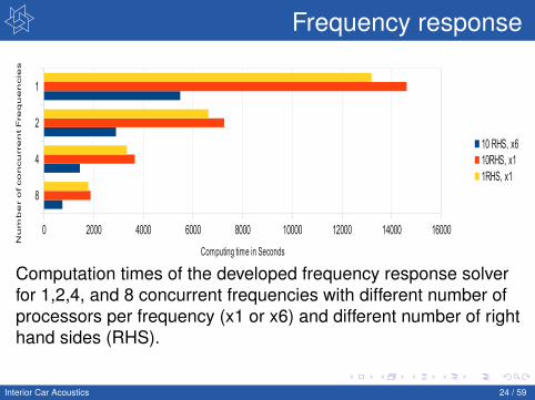
Frequency response

8

4

2

1

0 2000 4000 6000 8000 10000 12000 14000 16000

10 RHS, x610RHS, x11RHS, x1

Computing time in Seconds

Nu

mb

er o

f co

ncu

rre

nt F

re

qu

en

cie

s

1

Computation times of the developed frequency response solverfor 1,2,4, and 8 concurrent frequencies with different number ofprocessors per frequency (x1 or x6) and different number of righthand sides (RHS).


Eigenvalue tracking

−200 −100 0 1000

100

200

300

400

500

600

−200 −100 0 1000

100

200

300

400

500

600

1

2

3

1We use Krylov subspace methods with many different shifts: Atypical trapezoidal region – within which all eigenvalues aresought – at beginning and after three shifts have beenprocessed.


Intermediate conclusion

. Commercially available codes are not satisfactory.

. Discrete finite elements and quasi-uniform grids are a waste.

. For frequency analysis of high frequencies nothing reallyworks.

. So far everything is partially heuristic, we cannot guaranteethat we find all the desired eigenvalues.

. Eigenvalue methods need to use direct solvers forshift-and-invert.

. Homotopy and Newton like methods need to be developedand analyzed.

. Multi-way adaptive methods need to be developed, studiedand made industrially available.


Outline



Adaptive FEM for ev. comp.

. Adaptive finite element (AFEM) methods for PDE boundaryvalue problems are well studied. A priori and a posteriori errorestimates are available for many problems.

. For PDE eigenvalue problems the problem is much harder.

. Most results and methods only for the self-adjoint elliptic case.

. a priori estimates Larsson 2001, Knyazev et al. 2006, 2007,2008.

. a posteriori estimates Verführt 1996, Giani/Graham 2008,Carstensen/Gedicke 2008, Garau/Morin/Zuppa 2008.

. Nonsymmetric problems: Heuveline/Rannacher 2001,Rannacher 2009.

. Very few applications in industrial codes Zschiedrich, Burger,Pomplun, Schmidt 2007/2008.


Getting EVP AFEM into industrial practice

. Need to understand and analyze the non-selfadjoint case.

. Need proof of functionality, prototype for industrial problems.

. Need to match analytic adaptation concepts with numericallinear algebra and optimization adaption concepts.

. Need to make this useful on modern computer architectures.


Model problem: Elliptic PDE evp

Model problem:

∆u = λu in Ωu = 0 on ∂Ω

Classical FEM discretization (with mesh-width H) leads togeneralized discrete evp

AHuH = λHBHuH


Adaptive FEM

Solve→ Estimate→ Mark→ Refine

. In classical AFEM it is assumed that the algebraic evp issolved exactly.

. But this requires the largest percentage of the computing time.

. The solution of the algebraic evp is only used to determinewhere the grid is refined. This is a complete waste ofcomputational work.

. How we can incorporate the solution of the algebraiceigenvalue problem (AEVP) into the adaptation process?


AFEMLA

Solve:. compute eigenpair (λH , uH) on the coarse mesh,. use iterative solver, i.e. Krylov subspace method,. do not solve the problem very accurately, stop after k steps or

when tolerance tol is reached.Estimate:. prolongate uH from the coarse mesh TH to the uniformly

refined mesh Th,. compute residual vector rh and identify all its large coefficients

and corresponding basis functions (nodes).Mark and Refine: mark elements and refine the mesh.


Standard AFEM versus AFEMLA


Standard AFEM AFEMLA


Analysis

small residual vectorQ1?=⇒ good approximation of the discretized eigenpair (λH , uH)

Q2?=⇒ good approximation of the PDE eigenpair (λ,u)

Q1: yes. residual errors can be transformed to backward errors.. if eigenvalues are well-conditioned.

Q2: yes, if. saturation assumption holds, i.e., λh − λ ≤ β(λH − λ).

Computable bounds = backward error analysis + saturationassumption.


Backward error

TheoremLet A,B be n × n matrices and let B be invertible. Let λ be acomputed eigenvalue for the matrix pair (A,B), let x be anassociated normalized eigenvector, i.e., ‖x‖2 = 1, and letr = Ax − λBx. Then λ is an exact eigenvalue with associatedeigenvector x of a pair (A + E ,B), where ‖E‖2 = ‖r‖2.

Backward Error is of size of residual.


Error bounds

TheoremConsider a pair (A,B) of real n × n matrices and assume that Bis invertible. Let λ be a simple eigenvalue of the pair (A,B) withright eigenvector x and left eigenvector y, normalized so that‖x‖2 = ‖y‖2 = 1. Let λ = λ + δλ be the correspondingeigenvalue of the pair (A + E ,B) with eigenvector x = x + δx.Then

λ− λ =y∗Exy∗Bx

+ O(‖E‖22),

and|λ− λ| ≤ ‖E‖2

|y∗Bx |+ O(‖E‖2

2).


AFEMLA for smallest ev of Poisson evpRequire: An initial regular triangulation T i

H , a maximal number p ofArnoldi steps or a tolerance tol and a desired accuracy ε.

Ensure: Approximation λ1 to the smallest eigenvalue λ1 together withthe corresp. approx. eigenfunction u1.

1: Solve: Compute smallest eigenvalue λH and associatedeigenvector uH for algebraic evp on the coarse mesh T i

H . TerminteArnoldi after p steps or when a desired tolerance tol is reached.

2: Express uH using mesh T ih obtained by uniformly refining T i

H . Useprolongation P from mesh T i

H to mesh T ih , compute uh = PuH .

3: Estimate: Determine residual rh = Ahuh − λhBhuh for associatedev uh, identify large coeff. in rh and ass. (nodes).

4: if ‖rh‖ < ε then5: return (λh, uh)6: else7: Mark: Mark all edges of identif. nodes, apply closure algorithm.8: Refine: Refine coarse mesh T i

H to get T i+1H .

9: Start Algorithm 1 with T i+1H .

10: end ifInterior Car Acoustics 37 / 59

Computable bounds. λH : computed ev on coarse grid.. rH: Residual of eigenvector on coarse grid.. rH , uH : Prolongated residual, eigenvector on fine grid.. P Prolongation matrix, Bh fine mass matrix, β saturation

constant.

Theorem

|λH − λ|

≤ 11− β

(‖rH‖2‖B−1

H ‖2 +‖rH‖2 + ‖PT‖2‖rh‖2

‖PT Bhuh‖2+ ‖rh‖2‖B−1

h ‖2

)+ ‖rH‖2‖B−1

H ‖2.


Convergence on L-shape domain.


Approx. of smallest ev

ref. level #DOF A λ1 A |λ1 − λ1|1 5 13.1992 3.55952 27 10.8173 1.17753 99 9.9982 0.35844 306 9.7721 0.13235 641 9.6982 0.05856 1461 9.6652 0.02557 2745 9.6528 0.01318 5961 9.6455 0.0058


Conv. first 3 evs, L-shape domain.


Adaptive Mesh, first 3 evs


Outline



A simple nonsymmetric model problemCarstensen/Gedicke/M./Miedlar 2009Convection-diffusion eigenvalue problem:

−∆u + β · ∇u = λu in Ω and u = 0 on ∂Ω

Discrete weak primal and dual problem:

a(u`, v`) + c(u`, v`) = λ`b(u`, v`) for all v` ∈ V`,

a(w`,u?` ) + c(w`,u?` ) = λ?`b(w`,u?` ) for all w` ∈ V`.

Generalized algebraic eigenvalue problem:

(A` + C`)u` = λ`B`u` and u?`(A` + C`) = λ?`u?`B`

The eigenvalue with the smallest real part, which is proved to besimple and well separated Evans ’00, is considered.


Homotopy method

H(t) = (1− t)L0 + tL1 for t ∈ [0,1],

where L0u := −∆u and L1u := −∆u + β · ∇u. Discretehomotopy for the model eigenvalue problem:

H`(t) = (A` + C`)(t) = (1− t)A` + t(A` + C`) = A` + tC`.


Four errorsHomotopy, discretization, approximation and iteration error.Homotopy error:

|λ(1)− λ(t)| . (1− t)‖βL∞(Ω)‖‖u‖A = ν,

Discretization error:

‖λ(t)− λ`(t)‖ .∑T∈T`

(η2` (T ) + η?2

` (T )).

Approximation error:

|λ`(t)− λ`(t)|+ |λ?`(t)− λ?`(t)| ≤ µ`.

Iteration error The iterative eigensolver can be stopped when theerror is on the order of the others.


AFEM error

LemmaSuppose that |λ`(t)− λ`(t)| < 1. Then, for a fixed 0 ≤ t ≤ 1, theperturbation of the a posteriori error estimator for thediscretization error satisfies

‖η(λ`(t),u`(t),u?` (t))− η(λ`(t), u`(t), u?` (t))‖2. µ2(λ`(t), u`(t), u?` (t)).


Homotopy error

LemmaFor the model problem, the difference between the exacteigenvalues λ(t) of the homotopy H(t) and λ(1) can beestimated via

‖λ(1)− λ(t)‖ . ν(t) := (1− t)‖β∞‖ (|||u(t)|||+ |||u?(t)|||)

for 0 ≤ t ≤ 1. The constant in the inequality tends to1/(2b(u(1),u?(1)) as t → 1.


A posteriori error estimator

LemmaFor the model problem, the difference between the iterativeeigenvalue λ`(t) in the homotopy H`(t) and the continuouseigenvalue λ(1) of the original problem can be estimated aposteriori via

‖λ(1)− λ`(t)‖ . ν(λ`(t), u`(t), u?` (t)) + η2(λ`(t), u`(t), u?` (t))

+ µ2(λ`(t), u`(t), u?` (t))

in terms of

ν(λ`(t), u`(t), u?` (t)) := (1− t)|β|∞ (|||u`(t)|||+ |||u?` (t)|||)

+ (1− t)|β|∞(η(λ`(t), u`(t), u?` (t)) + µ(λ`(t), u`(t), u?` (t))

).


Adaptive homotopy algorithms


Algorithm 1: Balances the homotopy, discretization, iterationand approximation errors but uses fixed stepsize in continuationmethod.Algorithm 2: Adaptivity in homotopy and in the iteration isachieved by simple stepsize control, no homotopy error isconsidered.Algorithm 3: Adaptivity in the homotopy error, the discretizationerror, the iteration error including step size control.


Error dynamics


Figure: Conv. history of Algorithm 1, 2 and 3 with respect to #DOF.


Figure: Conv. history of Algorithm 1, 2 and 3 with respect to CPU time.


λ ≈ 44.739208802205724t η`(t) ν`(t) µ`(t) est. error

0.0000 23.0271 95.6366 0.2701265 118.933820.5000 32.6896 51.7112 0.0843690 84.485120.7500 11.6020 28.5244 0.4515713 40.578000.8750 6.7380 15.4099 0.4711298 22.619120.9375 7.8500 7.9782 0.0272551 15.855470.9688 3.2088 4.0697 0.2891100 7.567620.9844 1.2060 2.0673 0.4278706 3.701190.9922 0.4560 1.0380 0.0004539 1.494510.9961 0.4602 0.5202 0.0029006 0.983220.9980 0.1864 0.2608 0.0012530 0.448430.9990 0.0707 0.1305 0.0204610 0.221620.9995 0.0282 0.0653 0.0003639 0.093860.9998 0.0282 0.0326 0.0001766 0.061050.9999 0.0106 0.0163 0.0001521 0.027031.0000 0.0007 0.0000 0.0000243 0.00073


Errors and DOFst λ`(t)

|λ`(1)−λ`(t)||λ`(1)| #DOF CPU time

0.0000 22.86578 0.48891 25 0.760.5000 26.73866 0.40234 25 1.200.7500 32.54928 0.27247 55 1.550.8750 38.00079 0.15062 107 2.180.9375 40.73818 0.08943 107 3.070.9688 42.39339 0.05243 197 4.010.9844 43.77023 0.02166 385 6.060.9922 44.13547 0.01349 715 9.740.9961 44.32847 0.00918 715 16.590.9980 44.58151 0.00352 1398 23.570.9990 44.65025 0.00199 2494 37.140.9995 44.68298 0.00126 4848 66.700.9998 44.69522 0.00098 4848 119.470.9999 44.72311 0.00036 8785 175.751.0000 44.73615 0.00007 55235 226.87


Final mesh


What about the SFE problem ?

. Today there is no easy way to get adaptivity into the code.

. There is an urgent need to combine discrete FEM modellingand adaptivity.

. We need methods for nonlinear PDE eigenvalue problemswithin optimization loop.

. The mathematical theory and algorithms are still far from theneeds in reality.

. Commercially available codes are not satisfactory.

. Homotopy and Newton like methods need to be developedand analyze.

. Multi-way adaptive methods need to be developed, studiedand made industrially available.


References

. V. M. and A. Miedlar, Adaptive Computation of SmallestEigenvalues of Elliptic Partial Differential Equations,PREPRINT 565, DFG Research Center MATHEON. Hasappeared electronically in NUMERICAL LINEAR ALGEBRA WITHAPPLICATIONS 2010. DOI: 10.1002/nla.733

. C. Carstensen, J. Gedicke, V. M., and A. Miedlar, An adaptivehomotopy approach for non-selfadjoint eigenvalue problemsPREPRINT 718, DFG Research Center MATHEON. In revisionin NUMERISCHE MATHEMATIK.

. A. Miedlar, Inexact adaptive finite element methods for ellipticPDE eigenvalue problems, Dissertation, March 2011.


Thank you very muchfor your attention.


Numerical solution of eigenvalue problems in acoustic field

Documents

Transcript of Numerical solution of eigenvalue problems in acoustic field