Numerical Solution Methods - uni-wuerzburg.de · 36 Chapter 3 – Numerical Solution Methods...
50
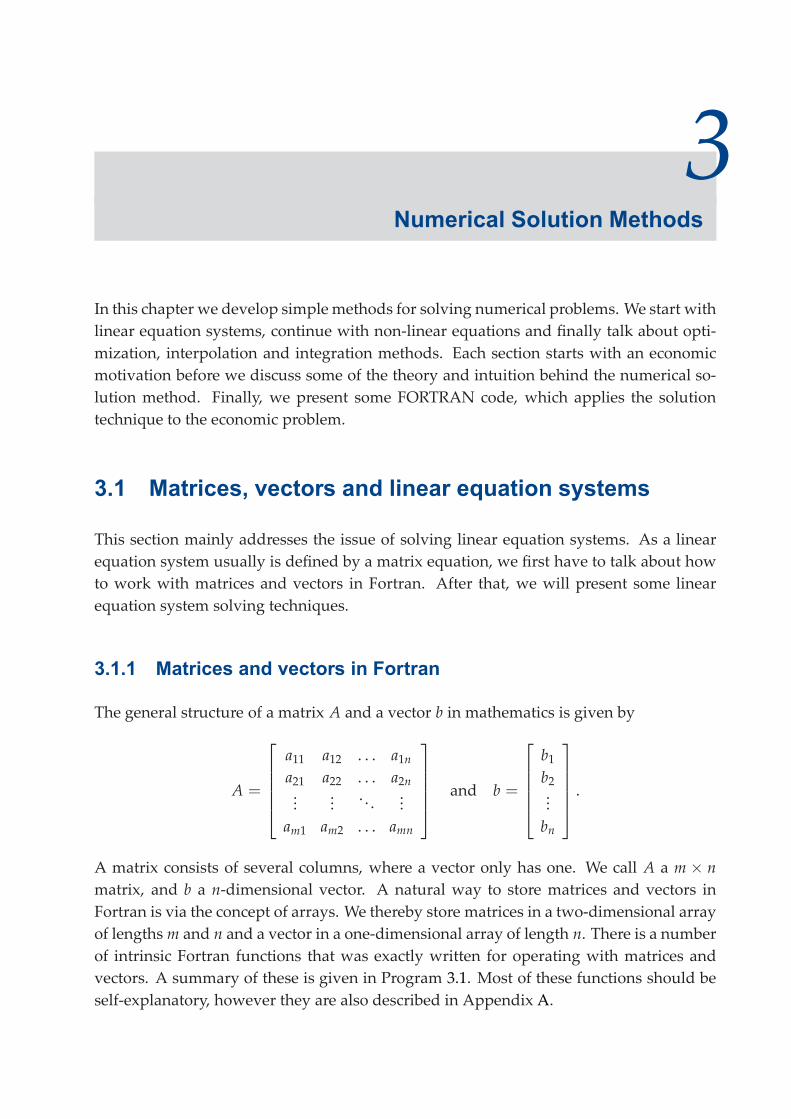
3 Numerical Solution Methods In this chapter we develop simple methods for solving numerical problems. We start with linear equation systems, continue with non-linear equations and finally talk about opti- mization, interpolation and integration methods. Each section starts with an economic motivation before we discuss some of the theory and intuition behind the numerical so- lution method. Finally, we present some FORTRAN code, which applies the solution technique to the economic problem. 3.1 Matrices, vectors and linear equation systems This section mainly addresses the issue of solving linear equation systems. As a linear equation system usually is defined by a matrix equation, we first have to talk about how to work with matrices and vectors in Fortran. After that, we will present some linear equation system solving techniques. 3.1.1 Matrices and vectors in Fortran The general structure of a matrix A and a vector b in mathematics is given by A = ⎡ ⎢ ⎢ ⎢ ⎢ ⎣ a 11 a 12 ... a 1n a 21 a 22 ... a 2n . . . . . . . . . . . . a m1 a m2 ... a mn ⎤ ⎥ ⎥ ⎥ ⎥ ⎦ and b = ⎡ ⎢ ⎢ ⎢ ⎢ ⎣ b 1 b 2 . . . b n ⎤ ⎥ ⎥ ⎥ ⎥ ⎦ . A matrix consists of several columns, where a vector only has one. We call A a m × n matrix, and b a n-dimensional vector. A natural way to store matrices and vectors in Fortran is via the concept of arrays. We thereby store matrices in a two-dimensional array of lengths m and n and a vector in a one-dimensional array of length n. There is a number of intrinsic Fortran functions that was exactly written for operating with matrices and vectors. A summary of these is given in Program 3.1. Most of these functions should be self-explanatory, however they are also described in Appendix A.
Transcript of Numerical Solution Methods - uni-wuerzburg.de · 36 Chapter 3 – Numerical Solution Methods...
3Numerical Solution Methods
In this chapter we develop simple methods for solving numerical problems. We start withlinear equation systems, continue with non-linear equations and finally talk about opti-mization, interpolation and integration methods. Each section starts with an economicmotivation before we discuss some of the theory and intuition behind the numerical so-lution method. Finally, we present some FORTRAN code, which applies the solutiontechnique to the economic problem.
3.1 Matrices, vectors and linear equation systems
This section mainly addresses the issue of solving linear equation systems. As a linearequation system usually is defined by a matrix equation, we first have to talk about howto work with matrices and vectors in Fortran. After that, we will present some linearequation system solving techniques.
3.1.1 Matrices and vectors in Fortran
The general structure of a matrix A and a vector b in mathematics is given by
A =
⎡⎢⎢⎢⎢⎣a11 a12 . . . a1na21 a22 . . . a2n...
... . . . ...am1 am2 . . . amn
⎤⎥⎥⎥⎥⎦ and b =
⎡⎢⎢⎢⎢⎣b1b2...bn
⎤⎥⎥⎥⎥⎦ .
A matrix consists of several columns, where a vector only has one. We call A a m × nmatrix, and b a n-dimensional vector. A natural way to store matrices and vectors inFortran is via the concept of arrays. We thereby store matrices in a two-dimensional arrayof lengths m and n and a vector in a one-dimensional array of length n. There is a numberof intrinsic Fortran functions that was exactly written for operating with matrices andvectors. A summary of these is given in Program 3.1. Most of these functions should beself-explanatory, however they are also described in Appendix A.

36 Chapter 3 – Numerical Solution Methods
Program 3.1: Matrix and vector operations
program matrices
implicit noneinteger :: i, jreal*8 :: a(4), b(4)real*8 :: x(2, 4), y(4, 2), z(2, 2)
! initialize vectors and matricesa = (/(dble(5-i), i=1, 4)/)b = a+4d0x(1, :) = (/1d0, 2d0, 3d0, 4d0/)x(2, :) = (/5d0, 6d0, 7d0, 8d0/)y = transpose(x)z = matmul(x, y)
! show results of different functionswrite(*,’(a,4f7.1/)’)’ vektor a = ’,(a(i),i=1,4)write(*,’(a,f7.1)’) ’ sum(a) = ’,sum(a)write(*,’(a,f7.1/)’) ’ product(a) = ’,product(a)write(*,’(a,f7.1)’) ’ maxval(a) = ’,maxval(a)write(*,’(a,i7)’) ’ maxloc(a) = ’,maxloc(a)write(*,’(a,f7.1)’) ’ minval(a) = ’,minval(a)write(*,’(a,i7/)’) ’ minloc(a) = ’,minloc(a)write(*,’(a,4f7.1)’) ’ cshift(a, -1) = ’,cshift(a,-1)write(*,’(a,4f7.1/)’)’ eoshift(a, -1) = ’,eoshift(a,-1)write(*,’(a,l7)’) ’ all(a<3d0) = ’,all(a<3d0)write(*,’(a,l7)’) ’ any(a<3d0) = ’,any(a<3d0)write(*,’(a,i7/)’) ’ count(a<3d0) = ’,count(a<3d0)write(*,’(a,4f7.1/)’)’ vektor b = ’,(b(i),i=1,4)write(*,’(a,f7.1/)’) ’ dot_product(a,b) = ’,dot_product(a,b)write(*,’(a,4f7.1/,20x,4f7.1/)’) &
’ matrix x = ’,((x(i,j),j=1,4),i=1,2)write(*,’(a,2f7.1,3(/20x,2f7.1)/)’)&
’ transpose(x) = ’,((y(i,j),j=1,2),i=1,4)write(*,’(a,2f7.1/,20x,2f7.1/)’) &
’ matmul(x,y) = ’,((z(i,j),j=1,2),i=1,2)
end program
3.1.2 Solving linear equation systems
In this section we want to show how to solve linear equation systems. There are twoways to solve those systems: by factorization or iterative methods. Both of these will bediscussed in the following.

3.1. Matrices, vectors and linear equation systems 37
Example Consider the supply and demand functions for three goods given by
qs1 = −10+ p1 qd1 = 20− p1 − p3qs2 = 2p2 qd2 = 40− 2p2 − p3qs3 = −5+ 3p3 qd3 = 10− p1 + p2 − p3
As one can see, the supply of the three goods only depends on their own price, while thedemand side shows strong price interdependencies. In order to solve for the equilibriumprices of the system we set supply equal to demand qsi = qdi in each market which afterrearranging yields the linear equation system
2p1 + p3 = 30
4p2 + p3 = 40
p1 − p2 + 4p3 = 15.
We can express a linear equation system in matrix notation as
Ax = b (3.1)
where x defines an n-dimensional (unknown) vector and A and b define a n× n matrixand a n-dimensional vector of exogenous parameters of the system. In the above example,we obviously have n = 3 and
A =
⎡⎢⎣ 2 0 1
0 4 11 −1 4
⎤⎥⎦ , x =
⎡⎢⎣ p1p2p3
⎤⎥⎦ and b =
⎡⎢⎣ 30
4015
⎤⎥⎦ .
Gaussian elimination and factorization
We now want to solve for the solution x of a linear equation system. Of course, if A wasa lower triangular matrix of the form
A =
⎡⎢⎢⎢⎢⎣a11 0 . . . 0a21 a22 . . . 0...
... . . . ...an1 an2 . . . ann
⎤⎥⎥⎥⎥⎦ ,
the elements of x could be easily derived by simple forward substitution, i.e.
x1 = b1/ a11x2 = (b2 − a21x1)/ a22
...
xn = (bn − an1x1 − an2x2 − · · · − ann−1xnn−1)/ ann.

38 Chapter 3 – Numerical Solution Methods
Similarly, the problem can be solved by backward substitution, if A was an upper trian-gular matrix. However, in most cases A is not triangular. Nevertheless, if a solution to theequation system existed, we could break up A into the product of a lower and upper tri-angular matrix, which means there is a lower triangular matrix L and an upper triangularmatrix U, so that A can be written as
A = LU.
If we knew these two matrices, equation (3.1) could be rearranged as follows:
Ax = (LU)x = L(Ux) = Ly = b.
Consequently, we first would determine the vector y from the lower triangular systemLy = b by forward substitution and then x via Ux = y using backward substitution.
Matrix decomposition
In order to factorize a matrix A into the components L and U we apply the Gaussianelimination method. In our example we can rewrite the Problem as
A =
⎡⎢⎣ 2 0 1
0 4 11 −1 4
⎤⎥⎦ =
⎡⎢⎣ 1 0 0
0 1 00 0 1
⎤⎥⎦
︸ ︷︷ ︸=L
×
⎡⎢⎣ 2 0 1
0 4 11 −1 4
⎤⎥⎦
︸ ︷︷ ︸=U
×
⎡⎢⎣ p1p2p3
⎤⎥⎦
︸ ︷︷ ︸=x
=
⎡⎢⎣ 30
4015
⎤⎥⎦
︸ ︷︷ ︸=b
.
We now want to transform L and U in order to make them lower and upper triangularmatrices. However, these transformations must not change the result x of the equationsystem LUx = b. It can be shown that subtracting the multiple of a row from anotherone satisfies this condition. Note that when we subtract a multiple of row i from row j inmatrix U, we have to add row i multiplied with the same factor to row j in matrix L.
In the above example, the first step is to eliminate the cells below the diagonal in the firstcolumn of U. In order to get a zero in the last row, one has to multiply the first row of Uby 0.5 and subtract it from the third. Consequently, we have to multiply the first row of Lwith 0.5 and add it to the third. After this first step matrices L and U are transformed to
L =
⎡⎢⎣ 1 0 0
0 1 00.5 0 1
⎤⎥⎦ and U =
⎡⎢⎣ 2 0 1
0 4 10 −1 3.5
⎤⎥⎦ .
In order to get a zero in the last row of the second column of U, we have to multiply thesecond row by -0.25 and subtract it from the third line. The entry in the last line and thesecond column of L then turns into -0.25. After this second step the matrices are
L =
⎡⎢⎣ 1 0 0
0 1 00.5 −0.25 1
⎤⎥⎦ and U =
⎡⎢⎣ 2 0 1
0 4 10 0 3.75
⎤⎥⎦ .

3.1. Matrices, vectors and linear equation systems 39
Now L and U have the intended triangular shape. It is easy to check that A = LU stillholds. Hence, the result of the equation systems LUx = b and Ax = b are identical.The above approach can be applied to any invertible matrix A in order to decompose itinto the L and U factors. We can now solve the system Ly = b for y by using forwardsubstitution. The solution to this system is given by
y1 = 30/ 1 = 30,
y2 = (40− 0 · 30)/ 1 = 40 and
y3 = (15− 0.5 · 30+ 0.25 · 40)/ 1 = 10.
Given the solution y = [30 40 10]T, the linear system Ux = y can then be solved usingbackward substitution, yielding the solution of the original linear equation, i.e.
x3 = 10/ 3.75 = 223,
x2 =(40− 1 · 22
3
)/4 = 9
13
and
x1 =(30− 0 · 91
3− 2
23
)/2 = 13
23.
The solution of a linear equation system via LU-decomposition is implemented in themodule matrixtools that accompanies this book. Program 3.2 demonstrates its use. Inthis program, we first include the matrixtoolsmodule and specify the matrices A, L,Uand the vector b. We then initialize A and b with the respective values given in the aboveexample. The subroutine lu_solve that comes along with the matrixtoolsmodule cannow solve the equation system Ax = b. The solution is stored in the vector b at the endof the subroutine. Alternatively, we could solely factorize A. This can be done with thesubroutine lu_dec. This routine receives a matrix A and stores the L andU factors in therespective variables. The output shows the same solution and factors as computed above.
The so-called L-U factorization algorithm is faster than other linear solution methodssuch as computing the inverse of A and then computing A−1b or using Cramer’s rule.Although L-U factorization is one of the best general method for solving a linear equa-tion system, situation may arise in which alternative methods may be preferable. Forexample, when one has to solve a series of linear equation systems which all have thesame A matrix but different b vectors, b1, b2, . . . , bm it is often computationally more effi-cient to compute and store the inverse of A and then compute the solutions x = A−1bj byperforming direct matrix vector multiplications.
Gaussian elimination can be accelerated for matrices possessing special structures. If Awas symmetric positive definite, A could be expressed as the product
A = LLT
of a lower triangular matrix L and its transpose. In this situation one can apply a specialform of Gaussian elimination, the so-called Cholesky factorization algorithm, which requires

40 Chapter 3 – Numerical Solution Methods
Program 3.2: Linear equation solving with matrixtools
program lineqsys
! modulesuse matrixtools
! variable declarationimplicit noneinteger :: i, jreal*8 :: A(3, 3), b(3)real*8 :: L(3, 3), U(3, 3)
! set up matrix and vectorA(1, :) = (/ 2d0, 0d0, 1d0/)A(2, :) = (/ 0d0, 4d0, 1d0/)A(3, :) = (/ 1d0, -1d0, 4d0/)b = (/30d0, 40d0, 15d0/)
! solve the systemcall lu_solve(A, b)
! decompose matrixcall lu_dec(A, L, U)
! outputwrite(*,’(a,3f7.2/)’)’ x = ’, (b(j),j=1,3)write(*,’(a,3f7.2/,2(5x,3f7.2/))’) &
’ L = ’,((L(i,j),j=1,3),i=1,3)write(*,’(a,3f7.2/,2(5x,3f7.2/))’) &
’ U = ’,((U(i,j),j=1,3),i=1,3)
end program
about half of the operations of the Gaussian approach. L is called the Cholesky factor orsquare root of A. Given the Cholesky factor of A, the linear equation
Ax = LLTx = L(LTx) = b
may be solved efficiently by using forward substitution to solve Ly = b and then back-ward substitution to solve LTx = y.
Another factorization methods decomposes A = QR, where Q is an orthogonalmatrix andR an upper triangular matrix. An orthogonal matrix has the property Q−1 = QT. Hence,the solution of the equation system can easily be computed by solving the system
Rx = QTb
via backward induction. However, computing aQR decomposition usually is more costlyand more complicated than the L-U factorization.

3.1. Matrices, vectors and linear equation systems 41
Matrix inversion
We can also invert matrices by using L-U factorization. Since A× A−1 = I, the inversionof a n× n matrix A is equivalent to successively computing the solution vectors xi of theequation systems
Axi = ei for i = 1, . . . , n,
where ei denotes the i-th unit vector, i.e. a vector with all entries being equal to zero, butthe i-th entry being equal to one. Defining a matrix in which the i-th column is equal tothe solution xi, we obtain the inverse of A, i.e.
A−1 =
⎡⎢⎣ | | |x1 x2 . . . xn| | |
⎤⎥⎦ .
A matrix inversion can be performed by means of the function lu_invert which alsocomes along the the matrixtools module. Program 3.3 shows how to do this. After
Program 3.3: Inversion of a matrix
program inversion
! modulesuse matrixtools
! variable declarationimplicit noneinteger :: i, jreal*8 :: A(3, 3), Ainv(3, 3), b(3)
! set up matrix and vectorA(1, :) = (/ 2d0, 0d0, 1d0/)A(2, :) = (/ 0d0, 4d0, 1d0/)A(3, :) = (/ 1d0, -1d0, 4d0/)b = (/30d0, 40d0, 15d0/)
! invert AAinv = lu_invert(A)
! calculate solutionb = matmul(Ainv, b)
! outputwrite(*,’(a,3f7.2/)’)’ x = ’, (b(j),j=1,3)write(*,’(a,3f7.2/,2(8x,3f7.2/))’) &
’ A^-1 = ’,((Ainv(i,j),j=1,3),i=1,3)
end program

42 Chapter 3 – Numerical Solution Methods
having specified A and b in this program, we compute the inverse of A with the functionlu_invert. The result is stored in the array Ainv. We then compute the solution of theabove equation system by multiplying Ainvwith b. The result is printed on the screen.
Iterative methods
The Gaussian elimination procedure computes an exact solution to the equation systemAx = b. However, the algorithm is quite unstable and sensitive to round-off errors. Aclass of more stable algorithms is the class of iterative methods such as the Jacobi or theGauss-Seidel approach. In opposite to factorization methods, both of these methods onlyyield approximations to the exact solution.
The basic idea of iterative methods is quite simple. Given the linear equation systemAx = b, one can choose any invertible matrix Q and rewrite the system as
Ax+Qx = b+Qx or
Qx = b+ (Q− A)x.
We therefore obtain
x = Q−1 [b+ (Q− A)x] = Q−1b+ (I − Q−1A)x.
If we let Q have a simple and easily invertible form, e.g. the identity matrix, we couldderive the iteration rule
xi+1 = Q−1b+ (I − Q−1A)xi.
It can be shown that, if the above iteration converges, it converges to the solution of linearequation system Ax = b.12
The Jacobi and the Gauss-Seidelmethod are popular representatives of the iteration meth-ods. While the Jacobi method sets Q equal to the diagonal matrix formed out of the di-agonal entries of A, the Gauss-Seidel method sets Q equal to the upper triangular matrixof upper triangular elements of A. Both of these matrices are easily invertible by hand.Program 3.3 shows how iterative methods can be applied to our problem.
When A becomes large and sparse, i.e. many entries of A are equal to zero, the conver-gence speed of both Jacobi and Gauss-Seidel method becomes quite slow. Therefore oneusually applies SOR-methods (successive overrelaxation), another representative of iter-ative methods. However, due to their higher complexity, we don’t want to discuss thesemethods in detail.
12 Convergence depends on the value of the matrix norm ||I −Q−1A|| which has to be smaller than 1.

3.1. Matrices, vectors and linear equation systems 43
Program 3.4: Jacobi approximation
program jacobi
! variable declarationimplicit noneinteger :: iter, ireal*8 :: A(3, 3), Dinv(3, 3), ID(3, 3), C(3, 3)real*8 :: b(3), d(3), x(3), xold(3)
! set up matrices and vectorsA(1, :) = (/ 2d0, 0d0, 1d0/)A(2, :) = (/ 0d0, 4d0, 1d0/)A(3, :) = (/ 1d0, -1d0, 4d0/)b = (/30d0, 40d0, 15d0/)
ID = 0d0Dinv = 0d0do i = 1,3
ID(i, i) = 1d0Dinv(i, i) = 1d0/A(i, i)
enddo
! calculate iteration matrix and vectorC = ID-matmul(Dinv, A)d = matmul(Dinv, b)
! initialize xoldxold = 0d0
! start iterationdo iter = 1, 200
x = d + matmul(C, xold)
write(*,’(i4,f12.7)’)iter, maxval(abs(x-xold))
! check for convergenceif(maxval(abs(x-xold)) < 1d-6)then
write(*,’(/a,3f12.2)’)’ x = ’,(x(i),i=1,3)stop
endif
xold = xenddo
write(*,’(a)’)’Error: no convergence’
end program

44 Chapter 3 – Numerical Solution Methods
3.2 Nonlinear equations and equation systems
One of the most basic numerical problems encountered in computational economics is tofind the solution to a nonlinear equation or a whole system of nonlinear equations. Anonlinear equation system usually can be defined by a function
f (x) : Rn → Rn
that maps an n dimensional vector x into the space Rn. We call the solution to the linearequation system f (x) = 0 a root of f . The root of a nonlinear equation system usuallyhas no closed-form solution. Consequently, various numerical methods addressing theissue of root-finding were invented. In this section, we introduce a very simple one-dimensional method called bisection search. As this method converges quite slow, weshow how to enhance speed by using Newton’s method. We then discuss some modi-fications of Newton’s algorithm and show the very general class of fixed-point iterationmethods. All those methods will, like in the previous section, be demonstrated with asimple example. We close the section by introducing a solver for multidimensional non-linear equation systems.
Example Suppose the demand function in a goods market is given by
qd(p) = 0.5p−0.2 + 0.5p−0.5,
where the first term denotes domestic and the second term export demand. Supplyshould be inelastic and given by qs = 2 units. At what price p∗ does the market clear?Setting supply equal to demand leads to the equation
0.5p−0.2 + 0.5p−0.5 = 2
which can be reformulated as
f (p) = 0.5p−0.2 + 0.5p−0.5 − 2 = 0. (3.2)
The second of the two equations exactly has the form f (p) = 0 described above. Themarket clearing price consequently is the solution to a nonlinear equation. Note that it isnot possible to derive an analytical solution to this problem. Hence, we need a numericalmethod to solve for p∗.
3.2.1 Bisection search in one dimension
A very intuitive and ad-hoc approach to solving nonlinear equations in one dimension isthe so-called bisection search. The basic idea behind this method is a mathematical theoremcalled intermediate value theorem. It states that, if [a, b] is an interval, f is a continuous

3.2. Nonlinear equations and equation systems 45
function and f (a) and f (b) have different signs, i.e. f (a) · f (b) < 0, then f has a rootwithin the interval [a, b]. The bisection algorithm now successively bisects the interval[a, b] into intervals of equal size and tests in which interval the root of f is located byusing the above theorem.
Specifically, the algorithm proceeds as follows: suppose we had an interval [ai , bi] withthe property that f (ai) · f (bi) < 0, i.e. f has a root within this interval. We now bisect thisinterval into the sub-intervals [ai , xi] and [xi, bi] with
xi =ai + bi
2.
We can now test in which interval the root of f is located and calculate a new interval[ai+1, bi+1] by
ai+1 = ai and bi+1 = xi if f (ai) · f (xi) < 0,
ai+1 = xi and bi+1 = bi otherwise.
Figure 3.1 demonstrates the approach.
ai
f(x)
x = ai i+1 x
f(x)
x*
bi = bi+1
Figure 3.1: Bisection search for finding the root of a function
Note that, due to the bisection of [ai, bi], we successively halve the interval size with everyiteration step. Consequently, xi converges towards the real root f (x∗) of f . We stopthe iteration process, if xi has sufficiently converged, i.e. the difference between twosuccessive values is smaller than an exogenously specified tolerance level ε
|xi+1 − xi| = |xi+1 − ai+1| = |xi+1 − bi+1| = 12i+2 |b0 − a0| < ε.

46 Chapter 3 – Numerical Solution Methods
Program 3.5 shows how to find the equilibrium price in the above example by usingbisection search.
Program 3.5: Bisection search in one dimension
program bisection
! variable declarationimplicit noneinteger :: iterreal*8 :: x, a, b, fx, fa, fb
! set initial guesses and function valuesa = 0.05d0b = 0.25d0fa = 0.5d0*a**(-0.2d0)+0.5d0*a**(-0.5d0)-2d0fb = 0.5d0*b**(-0.2d0)+0.5d0*b**(-0.5d0)-2d0
! check whether there is a root in [a,b]if(fa*fb >= 0d0)then
stop ’Error: There is no root in [a,b]’endif
! start iteration processdo iter = 1, 200
! calculate new bisection point and function valuex = (a+b)/2d0fx = 0.5d0*x**(-0.2d0)+0.5d0*x**(-0.5d0)-2d0
write(*,’(i4,f12.7)’)iter, abs(x-a)
! check for convergenceif(abs(x-a) < 1d-6)then
write(*,’(/a,f12.7,a,f12.9)’)’ x = ’,x,’ f = ’,fxstop
endif
! calculate new intervalif(fa*fx < 0d0)then
b = xfb = fx
elsea = xfa = fx
endifenddo
write(*,’(a)’)’Error: no convergence’
end program
3.2. Nonlinear equations and equation systems 47
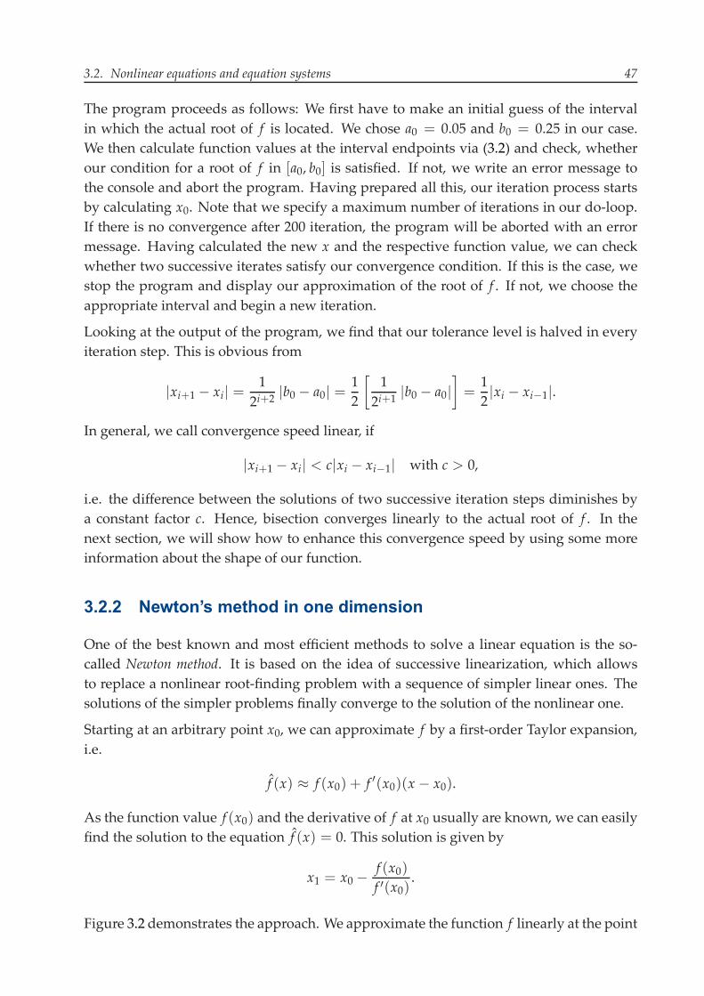
The program proceeds as follows: We first have to make an initial guess of the intervalin which the actual root of f is located. We chose a0 = 0.05 and b0 = 0.25 in our case.We then calculate function values at the interval endpoints via (3.2) and check, whetherour condition for a root of f in [a0, b0] is satisfied. If not, we write an error message tothe console and abort the program. Having prepared all this, our iteration process startsby calculating x0. Note that we specify a maximum number of iterations in our do-loop.If there is no convergence after 200 iteration, the program will be aborted with an errormessage. Having calculated the new x and the respective function value, we can checkwhether two successive iterates satisfy our convergence condition. If this is the case, westop the program and display our approximation of the root of f . If not, we choose theappropriate interval and begin a new iteration.
Looking at the output of the program, we find that our tolerance level is halved in everyiteration step. This is obvious from
|xi+1 − xi| = 12i+2 |b0 − a0| =
12
[1
2i+1 |b0 − a0|]=
12|xi − xi−1|.
In general, we call convergence speed linear, if
|xi+1 − xi| < c|xi − xi−1| with c > 0,
i.e. the difference between the solutions of two successive iteration steps diminishes bya constant factor c. Hence, bisection converges linearly to the actual root of f . In thenext section, we will show how to enhance this convergence speed by using some moreinformation about the shape of our function.
3.2.2 Newton’s method in one dimension
One of the best known and most efficient methods to solve a linear equation is the so-called Newton method. It is based on the idea of successive linearization, which allowsto replace a nonlinear root-finding problem with a sequence of simpler linear ones. Thesolutions of the simpler problems finally converge to the solution of the nonlinear one.
Starting at an arbitrary point x0, we can approximate f by a first-order Taylor expansion,i.e.
f̂ (x) ≈ f (x0) + f ′(x0)(x− x0).
As the function value f (x0) and the derivative of f at x0 usually are known, we can easilyfind the solution to the equation f̂ (x) = 0. This solution is given by
x1 = x0 − f (x0)f ′(x0)
.
Figure 3.2 demonstrates the approach. We approximate the function f linearly at the point

48 Chapter 3 – Numerical Solution Methods
x0
f(x)
f(x)^
x1 x
f(x)
x*
Figure 3.2: Newton’s method for finding the root of a function
x0 and find the solution x1 to the approximated equation system. x1 is now closer to thetrue solution x∗ of the equation f (x) = 0 than x0.
By defining the iteration rule
xi+1 = xi − f (xi)f ′(xi)
(3.3)
and starting with an initial guess x0, we therefore obtain a series of values x0, x1, x2, . . .that converges towards x∗. We again stop the iteration process, if xi has sufficiently con-verged, i.e.
|xi+1 − xi| =∣∣∣∣ f (xi)f ′(xi)
∣∣∣∣ < ε.
Program 3.6 demonstrates this approach. We first have to make an initial guess x0. Wechose 0.05 in our example. We then start the iteration process by calculating the functionvalue and the first derivative
f ′(p) = −0.1p−1.2 − 0.25p−1.5.
The new value xi+1 can then be computed from (3.3). We finally check for convergenceand stop the program, if convergence is reached. Else we store the value xi+1 and start anew iteration with it.
If we take a closer look at the output of this program, we see that, from iteration step 3 on-wards, the number of zeros in our tolerance level |xi+1 − xi| always doubles. Specifically,

3.2. Nonlinear equations and equation systems 49
Program 3.6: Newton’s method in one dimension
program newton
! variable declarationimplicit noneinteger :: iterreal*8 :: xold, x, f, fprime
! set initial guessxold = 0.1d0
! start iteration processdo iter = 1, 200
! calculate function valuef = 0.5d0*xold**(-0.2d0)+0.5d0*xold**(-0.5d0)-2d0
! calculate derivativefprime = -0.1d0*xold**(-1.2d0)-0.25d0*xold**(-1.5d0)
! calculate new valuex = xold - f/fprime
write(*,’(i4,f12.7)’)iter, abs(x-xold)
! check for convergenceif(abs(x-xold) < 1d-6)then
write(*,’(/a,f12.7,a,f12.9)’)’ x = ’,x,’ f = ’,fstop
endif
! copy old valuexold = x
enddo
write(*,’(a)’)’Error: no convergence’
end program
it can be shown that
|xi+1 − xi| < c|xi − xi−1|2
with a certain c > 0 holds, if xi is sufficiently close to the true solution of f (x) = 0 andthe iteration process converges. We call this convergence property quadratic convergence.This convergence speed obviously is much faster than the linear speed of bisection search.
However, Newton’s methods also comes with disadvantages. One of them obviouslyis that f has to be continuously differentiable at least once, for quadratic convergence

50 Chapter 3 – Numerical Solution Methods
even twice. In addition, one has to keep in mind that Newton’s algorithm not necessarilyconverges to the root of f . There are several properties a function can have that preventconvergence of the iteration process. If for example f has an extrem value near the rootx∗ it might be that one iterate xi is very close to this value. Consequently, the derivativef ′(xi) gets close to zero and the calculation in (3.3) might lead to an error. Furthermore, iff has an inflection point, a situation like on the left side of Figure 3.3 might arise, wherethe iterated values jump from a left to a right point and back. Last, if f is not defined for
f(x)
x
f(x)
xi
x* xi+1
f(x)
x
f(x)
x* xixi+1
Figure 3.3: Convergence problems in Newton’s algorithm
every x ∈ R, like e.g. log(x) in the right part of Figure 3.3, we might jump outside thedefined area of f while iterating. This problem, however, can often be solve by choosingdifferent initial guesses for the starting value of the Newton procedure.
Sometimes it is quite difficult to calculate the derivative of f analytically. If this is thecase, one usually approximates the derivative by a secant, i.e.
f ′(xi) ≈ f (xi)− f (xi−1)
xi − xi−1.
The iteration procedure in (3.3) then turns into
xi+1 = xi − xi − xi−1
f (xi)− f (xi−1)f (xi).
This method is called secant method. Note that we now need two starting values x0 and x1in order to start the iteration process. It can be shown that in terms of convergence speed,the secant method iteration values follow
|xi+1 − xi| = c|xi − xi−1|1.6.Consequently, convergence speed is somewhat in between linear and quadratic. How-ever, the advantage of the secant method is that in every iteration only one function value

3.2. Nonlinear equations and equation systems 51
f (xi) has to be calculated. In opposite to that, the original Newton procedure needs tocalculate f (xi) and f ′(xi), hence, two function values. Consequently, if we combine twosteps of the secant procedure to one in order to reach comparability, we obtain the con-vergence speed
|xi+1 − xi| = c|c|xi−1 − xi−2|1.6|1.6 = c2.6|xi−1 − xi−2|2.56.Therefore, the secant method in general is more efficient than Newton’s algorithm. Fur-thermore it is easier to implement, as we do not need to calculate the derivative of f .
3.2.3 Fixed-point iteration methods
The last and most general class of methods we want to introduce for solving one-dimen-sional, nonlinear equations is the class of fixed-point iteration methods. This method isbased on a reformulation of the nonlinear equation. Suppose we transform f (x) = 0 bymultiplying with σ and adding x on both sides into
x = x+ σ f (x) =: g(x).
Obviously, the solution x∗ to this equation is a fixed-point of g(·) and in addition f (x∗) =0 holds if σ �= 0. Hence, the solution to the fixed point equation x = g(x) also is thesolution to the nonlinear equation f (x) = 0.
The fixed point iteration now is defined by
xi+1 = g(xi) = xi + σ f (xi).
It can be shown that a fixed point iteration procedure converges, if |g′(x∗)| < 1 and theinitial guess x0 is close enough to the root x∗ of f . Convergence speed of a fixed-pointiteration strongly depends on the function g, i.e. we have
|xi+1 − xi| = c|xi − xi−1|p
if the first p− 1 derivatives of g at x∗ are zero and the pth derivative is not equal to zero.As in general g′(x∗) = 1+ σ f ′(x∗) �= 0, the above fixed-point iteration will converge lin-early towards the actual root of f . It therefore is quite slow, however, easy to implement.Program 3.7 shows the fixed-point iteration method for our example.
The key question in a fixed-point iteration is how to choose σ. Usually one has to trydifferent values for σ. The rule of thumb is that the lower σ the slower the method con-verges. However, if σ is too large, it might happen that the method doesn’t convergeat all. Hence, choosing an appropriate σ is quite complicated and therefore, fixed-pointiteration is not used very often.
We want to close this section with a small remark. Note that Newton’s method
xi+1 = xi − f (xi)f ′(xi)
=: g(xi)
52 Chapter 3 – Numerical Solution Methods
Program 3.7: Fixed-point iteration in one dimension
program fixedpoint
! variable declarationimplicit noneinteger :: iterreal*8 :: xold, x, f, sigma
! set initial guess and chose sigmaxold = 0.05d0sigma = 0.2d0
! start iteration processdo iter = 1, 200
! calculate function valuef = 0.5d0*xold**(-0.2d0)+0.5d0*xold**(-0.5d0)-2d0
! calculate new valuex = xold + sigma*f
write(*,’(i4,f12.7)’)iter, abs(x-xold)
! check for convergenceif(abs(x-xold) < 1d-6)then
write(*,’(/a,f12.7,a,f12.9)’)’ x = ’,x,’ f = ’,fstop
endif
! copy old valuexold = x
enddo
write(*,’(a)’)’Error: no convergence’
end program
also is a fixed-point iteration procedure. With
g′(xi) =f (xi) f ′′(xi)[ f ′(xi)]2
= 0 and g′′(xi) =f ′′(xi)f ′(xi)
�= 0,
this fixed-point iteration procedure converges quadratically. Consequently, it might bepossible to construct methods that converge even faster than Newton’s algorithm bychoosing an appropriate fixed-point iteration procedure. However, up to now, proce-dures that can be run with acceptable effort have only been found for very special casesof functions f .

3.2. Nonlinear equations and equation systems 53
3.2.4 Multi-dimensional nonlinear equation systems
For multi-dimensional equation systems, solution methods become quite complicated.We therefore don’t want to discuss the theory in detail. For finding the root of a multi-dimensional equation system we use the so-called Broyden’s method, which is the mostpopular multivariate generalization of the univariate secant method. This method is alsocalled aQuasi-NewtonMethod as it approximates the Jacobi matrix of f in order to find thefunction’s root. For demonstrating the use of Broydn’s algorithm we consider anotherexample.
Example Two firms compete in a simple Cournot duopoly with the inverse demandand the cost functions
P(q) = q−1/ η Ck(qk) =ck2q2k with q = q1 + q2
for firm k = 1, 2. Given the profit functions of the two firms
Πk(q1, q2) = P(q1 + q2)qk − Ck(qk)
each firm i takes the other firm’s output as given and chooses it’s own output level inorder to solve
∂Πk
∂qk= f (q) = (q1 + q2)−1/ η − 1
η(q1 + q2)−1/ η−1qk − ckqk = 0 with k = 1, 2.
Broydn’smethod is implemented in the subroutine fzero contained in themodule rootfinding.This function can be applied to both one- and multi-dimensional problems. Program 3.8shows how to do this. Hereby, cournot is a function that returns exactly the values of thetwo marginal profit equations, see the program in the program folder. Again, we have touse an interface construct to include the external function cournot into our program.In addition, we have to include the module rootfindingwhich provides the subroutinefzero. Before we call this subroutine, we have to make an initial guess for the quan-tity vector q. We then let fzero search the root of the function cournot, which specifiesthe equations for our oligopoly quantities. In addition to the price vector and the func-tion, we hand a logical variable check to the subroutine. If anything goes wrong in it orthe iteration process does not converge, check will get the value .true., else .false..Given η = 1.6, c1 = 0.6 and c2 = 0.8 the program yields the solutions q1 = 0.8396 andq2 = 0.6888. We now can change the exogenous parameter values for η, c1, c2 and checkhow this affects the solution.
54 Chapter 3 – Numerical Solution Methods
Program 3.8: Fixed-point iteration in one dimension
program oligopoly
! modulesuse rootfinding
! variable declaration and interfaceimplicit nonereal*8 :: q(2)logical :: check
interfacefunction cournot(q)
real*8, intent(in) :: q(2)real*8 :: cournot(size(q, 1))
end functionend interface
! initialize qq = 0.1d0
! find rootcall fzero(q, cournot, check)
if(check)stop ’Error: fzero did not converge’
write(*,’(/a)’)’ Output’write(*,’(a,f10.4)’)’Firm 1: ’,q(1)write(*,’(a,f10.4)’)’Firm 2: ’,q(2)write(*,’(/a,f10.4)’)’Price : ’,(q(1)+q(2))**(-1d0/1.6d0)
end program

3.3. Function minimization 55
3.3 Function minimization
Beneath the problem of root-finding, minimizing functions constitutes a major problemin computational economics. Let
f (x) : X → R
a function that maps an n-dimensional vector x ∈ X ⊆ Rn into the real line R. Then thecorresponding minimization problem is defined as
minx∈X
f (x).
Note that minimization and maximization do not have to be considered separately, asminimizing the function − f (x) is exactly equal to its maximization. Obviously, mini-mization is very closely related to root-finding, as the derivative of a function becomeszero in a minimum. Consequently, if derivatives can be easily calculated, root-finding isa fair alternative to using a minimization method. However there are cases where usinga minimization method is superior, e.g. if derivatives can’t be calculated in a reasonableamount of time. In addition, non-differentiability of f eliminates the option of choos-ing a root-finding instead of a minimization algorithm. Last but not least, minimizationmethods often give us the possibility of constraining the set of possible values for x. Thisis obviously not possible with root-finding algorithms. Figure 3.4 addresses this issue.Looking for the unconstraint minimum of f , we can see that we could use either a root
f(x)
x
f(x)
a bx*
f‘(x)
Figure 3.4: Constraint minimization
finding or a minimization algorithm. However, if we would like to find the minimum off only on the interval [a, b], root-finding will not help us, as f ′ is positive on the wholeinterval. A constraint minimization method could however give us the actual solution ato this problem.

56 Chapter 3 – Numerical Solution Methods
Example A household can consume two goods x1 and x2. He values the consumptionof those goods with the joint utility function
u(x1, x2) = x0.41 + (1+ x2)0.5.
Here x2 acts as a luxury good, i.e. the household will only consume x2, if his availableresourcesW are large enough. x1 on the other hand is a normal good and will always beconsumed. Naturally, we have to assume that x1, x2 ≥ 0. With the prices for the goodsbeing p1 and p2, the households has to solve the optimization problem
maxx1,x2≥0
x0.41 + (1+ x2)0.5 s.t. p1x1 + p2x2 = W.
Note that there is no analytical solution to this problem.
Due to marginal utility increasing to ∞ with x1 approaching zero, the optimal x1 willalways be strictly larger than zero. However, we might result in a corner solution x2 = 0.As the set of allowed values for x2 is constraint, we will not be able to use a root-findingmethod to solve for the optimal choice of x1 and x2. Hence, we need a minimizationroutine. When using a minimization algorithm with an equality constraint, it is alwaysuseful to first plug in the constraint into the utility function and therefore reduce thedimension of the optimization problem. We therefore reformulate the above problem to
maxx2≥0
[W − p2x2
p1
]0.4+ (1+ x2)0.5.
This problem can be solved with various minimization routines.
3.3.1 The Golden-Search method
The Golden-Search method minimizes a one-dimensional function on the initially definedinterval [a, b]. The ideas behind this method is quite similar to the one of bisectionsearch. Golden-Search however divides in each iteration i the interval [ai , bi] into twosub-intervals by using the points xi,1 and xi,2 which satisfy the conditions
xi,2 − ai = bi − xi,1 andxi,1 − aibi − ai =
xi,2 − xi,1bi − xi,1 .
Consequently, xi,1 and xi,2 are computed from
xi,j = ai + ωj(bi − ai) with ω1 =3−√
52
≈ 0.382 and ω2 = 1− ω1 =
√5− 12
.
(3.4)
We now compute the function values f (xi,j) for j = 1, 2 and compare them. The nextiteration’s interval is then chosen according to
ai+1 = ai and bi+1 = xi,2 if f (xi,1) < f (xi,2),

3.3. Function minimization 57
ai+1 = xi,1 and bi+1 = bi otherwise.
The idea behind this iteration rule is quite simple. If f (xi,1) < f (xi,2), the lower values off will be located near xi,1, not xi,2. Consequently, one chooses the interval [ai , xi,2] as newiteration interval and therefore rules out the greater values of f , see Figure 3.5.
f(x)
x
f(x)
a = ai i+1 bix* xi,1 x =i,2 bi+1
Figure 3.5: Golden search method for finding minima
Program 3.9 shows how to apply the Golden-Search method to the above problem. At thebeginning of the program we choose values for the model parameter p1, p2 andW. We as-sume the price of the luxury good to be twice the price of the normal good and normalizethe available resources W = 1. We then have to set the starting interval. Note that set-ting a = 0 restricts x2 to be non-negative. b is finally initialized in a way that guaranteesthe consumption of good 1 to be positive for any x2 ∈ [a, b]. In the iteration process wecalculate xi,1 and xi,2 and the respective function values as shown in (3.4). Note that wealways use the negative of the actual function value in order to assure that we maximizehousehold’s utility. In opposite to the previous section, we define our tolerance level as|bi − ai|. This is because we now have two values xi,1 and xi,2 in every iteration and don’tknow which one to choose as approximation to our minimum x∗. Consequently, tak-ing the interval width of [ai, bi] as tolerance criterion insures that we can take any valuewithin this interval and meet our tolerance criterion. If our criterion is satisfied, we printthe minimum and the respective function value on the console. If not, we set the newiteration’s interval [ai+1, bi+1] according to the above iteration rule.
Taking a look at the output of the program, we find that x1 = 1 and x2 = 0 is the optimalsolution to our optimization problem. This indicates that the constraint x2 > 0 is actuallybinding for this price and resource combination. We can test this by extending the initialinterval [a, b] and setting a = -0.9d0 instead of 0. Doing this, Golden-Search returnthe unconstraint optimum x1 ≈ 1.61 and x2 ≈ −0.31 of the optimization problem inour example. Note that, similar as in the bisection search method, convergence speed ofGolden-Search is linear.

58 Chapter 3 – Numerical Solution Methods
Program 3.9: Golden-Search method in one dimension
program golden
! variable declarationimplicit nonereal*8, parameter :: p(2) = (/1d0, 2d0/)real*8, parameter :: W = 1d0
real*8 :: a, b, x1, x2, f1, f2integer :: iter
! initial interval and function valuesa = 0d0b = (W-p(1)*0.01d0)/p(2)
! start iteration processdo iter = 1, 200
! calculate x1 and x2 and function valuesx1 = a+(3d0-sqrt(5d0))/2d0*(b-a)x2 = a+(sqrt(5d0)-1d0)/2d0*(b-a)f1 = -(((W-p(2)*x1)/p(1))**0.4d0+(1d0+x1)**0.5d0)f2 = -(((W-p(2)*x2)/p(1))**0.4d0+(1d0+x2)**0.5d0)
write(*,’(i4,f12.7)’)iter, abs(b-a)
! check for convergenceif(abs(b-a) < 1d-6)then
write(*,’(/a,f12.7)’)’ x_1 = ’,(W-p(2)*x1)/p(1)write(*,’(a,f12.7)’)’ x_2 = ’,x1write(*,’(a,f12.7)’)’ u = ’,-f1stop
endif
! get new valuesif(f1 < f2)then
b = x2else
a = x1endif
enddo
end program
3.3.2 Brent’s and Powell’s algorithms
The problem with Golden-Search is it’s slow convergence. Therefore the function f iscalled quite often. For well-behaved functions a more sophisticated algorithm is based onBrent’s method. It relies on parabolic approximations f̂ of the actual function f . Finding the
3.3. Function minimization 59
minimum of a parabola is quite easy. If the parabola is given by f̂ (x) = c0 + c1x+ c2x2,then its minimum is located at
x = − c12c2
.
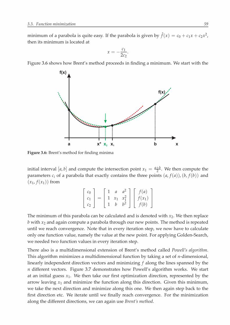
Figure 3.6 shows how Brent’s method proceeds in finding a minimum. We start with the
f(x)
x
f(x)
a bx* x1x2
Figure 3.6: Brent’s method for finding minima
initial interval [a, b] and compute the intersection point x1 = a+b2 . We then compute the
parameters ci of a parabola that exactly contains the three points (a, f (a)), (b, f (b)) and(x1, f (x1)) from ⎡
⎢⎣ c0c1c2
⎤⎥⎦ =
⎡⎢⎣ 1 a a2
1 x1 x211 b b2
⎤⎥⎦⎡⎢⎣ f (a)f (x1)f (b)
⎤⎥⎦
The minimum of this parabola can be calculated and is denoted with x2. We then replacebwith x2 and again compute a parabola through our new points. The method is repeateduntil we reach convergence. Note that in every iteration step, we now have to calculateonly one function value, namely the value at the new point. For applying Golden-Search,we needed two function values in every iteration step.
There also is a multidimensional extension of Brent’s method called Powell’s algorithm.This algorithm minimizes a multidimensional function by taking a set of n-dimensional,linearly independent direction vectors and minimizing f along the lines spanned by then different vectors. Figure 3.7 demonstrates how Powell’s algorithm works. We startat an initial guess x1. We then take our first optimization direction, represented by thearrow leaving x1 and minimize the function along this direction. Given this minimum,we take the next direction and minimize along this one. We then again step back to thefirst direction etc. We iterate until we finally reach convergence. For the minimizationalong the different directions, we can again use Brent’s method.

60 Chapter 3 – Numerical Solution Methods
x1
Figure 3.7: Powell’s algorithm for finding minima in multi dimensions
Both Brent’s and Powell’s method are included in the module minimization. It containsa subroutine fminsearch that is called with five arguments. Program 3.10 demonstratesits use taking the above example. The program also incorporates a module globals thatstores the parameters p1, p2 andW of the model. We also have to define a function thatwe want fminsearch to minimize. The function utility exactly matches the declaredinterface and returns the negative of the utility function u(x1, x2). Note that, if we wantedto define a multidimensional optimization problem, we would have declared the inputvariable x to the function as an assumed-size vector by using x(:). We now set the opti-mization interval borders a and b and make an initial guess x. fminsearch is then calledwith the initial guess x, a scalar f in which the function value in the minimum is stored,the interval borders and the function to minimize. The solution of the minimization prob-lem is returned in x. If we had a multi-dimensional problem, a and b should be vectorsof the same size as x. The result if finally printed on the console.
3.3.3 The problem of local and global minima
Unfortunately, there is no guarantee that a minimization method will find the global mi-nimum of a function. It might well be that one ends in a local minimum. Figure 3.8shows this problem with Golden-Search. We can see that f has a local minimum on theleft and the global minimum on the right side of the optimization interval [a, b]. Whenwe perform the first step of Golden-Search, we calculate the points x1 and x2 and therespective function values. For a next iteration’s optimization interval, we would thenchoose [a, x1], as f (x1) < f (x2). Obviously, with this step, we have already eliminatedthe chance of finding the global minimum, as after the first step we concentrate on the left

3.3. Function minimization 61
Program 3.10: Brent and Powell for finding minima
program brentmin
! modulesuse globalsuse minimization
! variable declaration and interfaceimplicit none
real*8 :: x, f, a, b
interfacefunction utility(x)
real*8, intent(in) :: xreal*8 :: utility
end functionend interface
! initial interval and function valuesa = 0d0b = (W-p(1)*0.01d0)/p(2)
! set starting pointx = (a+b)/2d0
! call minimizing routinecall fminsearch(x, f, a, b, utility)
! outputwrite(*,’(/a,f12.7)’)’ x_1 = ’,(W-p(2)*x)/p(1)write(*,’(a,f12.7)’)’ x_2 = ’,xwrite(*,’(a,f12.7)’)’ u = ’,-f
end program
hand side of the interval [a, b].
An easily implementable approach to overcome this problem is to first divide the originalinterval [a, b] into n sub-intervals [xi, xi+1] of equal size with x1 = a and xn+1 = b. Onevery of these sub-intervals, one then performs a full minimization procedure to find theminimum x∗i of f on the interval [xi, xi+1]. Now we have a set of minima {x∗i }ni=1. Ourglobal minimum finally is the value x∗i with the smallest function value f (x∗i ).
Figure 3.9 demonstrates the approach. We used a division into five intervals in this case.The green dots mark the local minima on the sub-intervals. We can see that the globalminimum is also contained in this set. Hence, with this procedure, we are able to findthe global minimum of a function. Note, however, that the procedure is quite costly, aswe have to perform 5 minimizations instead of only one. Consequently, it should only be

62 Chapter 3 – Numerical Solution Methods
x2x1
f(x)
x
f(x)
a bx*
Figure 3.8: The problem of local minima
x2 x3 x4 x5
f(x)
x
f(x)
a bx*
x *1x *2
x *3
x *4
x *5
Figure 3.9: Sub-interval division for solving the problem of local minima
used when one is sure that the problem of local optima may arise.

3.4. Numerical integration 63
3.4 Numerical integration
In many economic applications it is necessary to compute the definite integral of a real-valued function f with respect to a "weight" function w over an interval [a, b], i.e.
I( f ) =∫ b
aw(x) f (x) dx.
The weight function may be the identity function w(x) = 1, so that the integral representsthe area under the function f in the interval. In other applications the weight functioncould also be the probability density function of a continuous random variable x̃ withsupport [a, b], so that I( f ), represents the expected value of f (x̃).
In the following we discuss so-called numerical quadrature methods. In order to approxi-mate the above integral, quadrature methods choose a discrete set of quadrature nodes xiand appropriate weights wi in a way that
I( f ) ≈n
∑i=0wi f (xi).
The integral is therefore approximated by the sum of function values at the nodes a ≤x0 < · · · < xn ≤ b and the respective quadrature weights wi. Of course, the approxima-tion improves with a rising number n.
Different quadrature methods only differ with respect to the chosen nodes xi and weightswi. In the following we will concentrate on Newton-Cotesmethod and Gaussian quadraturemethod. The former approximates the integrand f between nodes using low-order poly-nomials and sum the integrals of the polynomials to estimate the integral of f . The lattermethods choose the nodes and weights in order to match specific moments (such as ex-pected value, variance etc.) of the approximated function.
3.4.1 Summed Newton-Cotes methods
In this section we set w(x) = 1. A weighted integral can then simply be computed bysetting g(x) = w(x) f (x) and approximating∫ b
ag(x) dx.
Summed Newton-Cotes formulas partition the interval [a, b] into n subintervals of equallength h by computing the quadrature nodes
xi := a+ ih, i = 0, 1, . . . , n, mit h :=b− an
.
A summed Newton-Cotes formula of degree k then interpolates the function f on everysubinterval [xi, xi+1] with a polynomial of degree k. We finally integrate the interpolatingpolynomial on every sub-interval and sum up all the resulting sub-areas. Figure 3.10shows this approach for k = 0 and k = 1.

64 Chapter 3 – Numerical Solution Methods
x2 x3 x4 x5
f(x)
x
f(x)
a = x1 b = x6
f(x)
x
f(x)
x2 x3 x4 x5a = x1 b = x6
Figure 3.10: Summed Newton-Cotes formulas for k = 0 and k = 1
Summed rectangle rule If k = 0, the interpolating functions are polynomials of degree0, i.e. constant functions. We can write any area below this constant functions on theinterval [xi, xi+1] as
I(0)[xi,xi+1]
( f ) = (xi+1 − xi) f (xi) = h f (xi),
which is the surface of a rectangle. The degree 0 formula is therefore called the summedrectangle rule, the explicit form of which is given by
I(0)( f ) =n−1
∑i=0h f (xi).
The weights of the summed rectangle rule consequently are
wi = h for i = 0, . . . , n− 1 and wn = 0.
Summed trapezoid rule If k = 1, the function f in the i-th subinterval [xi, xi+1] is ap-proximated by the line segment passing through the two points (xi, f (xi)) and (xi+1, f (xi+1)).The area under this line segment is the surface of a trapezoid, i.e.
I(1)[xi,xi+1]
( f ) = h f (xi) +12h[ f (xi+1)− f (xi)] =
h2[ f (xi) + f (xi+1)] .
It is immediately clear that the summed trapezoid rule improves the approximation of I( f )compared to the summed rectangle rule discussed above. Summing up the areas of thetrapezoids across sub-intervals yields the approximation
I(1) =h2
{f (a) + 2
n−1
∑i=1
f (xi) + f (b)
}
of the whole integral I( f ). The weights of the rule therefore are
w0 = wn =h2
and wi = h for i = 1, . . . , n− 1. (3.5)

3.4. Numerical integration 65
Summed rectangle and trapezoid rule are simple and robust. Hence, computation doesnot need much effort. In addition, the accuracy of the approximation of I( f ) increaseswith rising n. It is also clear that the trapezoid rule will exactly compute the integral ofany first-order polynomial, i.e. a line.
Program 3.11 shows how to apply the summed trapezoid rule to the function cos(x). We
Program 3.11: Summed trapezoid rule with cos(x)
program NewtonCotes
! variable declarationimplicit noneinteger, parameter :: n = 10
real*8, parameter :: a = 0d0, b = 2d0real*8 :: h, x(0:n), w(0:n), f(0:n)integer :: i
! calculate quadrature nodesh = (b-a)/dble(n)x = (/(a + dble(i)*h, i=0,n)/)
! get weightsw(0) = h/2d0w(n) = h/2d0w(1:n-1) = h
! calculate function values at nodesf = cos(x)
! Output numerical and analytical solutionwrite(*,’(a,f10.6)’)’ Numerical: ’,sum(w*f, 1)write(*,’(a,f10.6)’)’ Analytical: ’,sin(2d0)-sin(0d0)
end program
thereby first declare all the variables needed. Special attention should be devoted to thedeclaration of x, w and f. These arrays will store the quadrature nodes xi, the weights wiand the function values at the nodes f (xi), respectively. We then first compute h and thenodes xi = a+ ih and the weights wi as in (3.5). With the respective function values, theapproximation to the integral
∫ 2
0cos(x) dx = sin(2)− sin(0)
is the given by sum(w*f, 1). Note that the approximation of the integral is quite bad. Ifwe increase the number of quadrature nodes n increases the accuracy, however, we needabout 600 nodes in order to perfectly match numerical and analytical result on 6 digits.

66 Chapter 3 – Numerical Solution Methods
Summed Simpson rule Finally if k = 2, the integrand f in the i-th subinterval [xi, xi+1]
is approximated by a second-order polynomial function c0+ c1x+ c2x2. Now three graphpoints are required to specify the polynomial parameters ci in the subintervals. Giventhese parameters, one can compute the integral of the quadratic function in the subinter-val [xi, xi+1] as
I(2)[xi,xi+1]
( f ) =h3
[f (xi) + 4 f
(xi + xi+1
2
)+ f (xi+1)
].
Summing up the different areas on the sub-intervals yields
I(2)( f ) =h6
{f (a) + 2
n−1
∑i=1
f (xi) + 4n−1
∑i=0
f(xi + xi+1
2
)+ f (b)
}.
The summed Simpson rule is almost as simple to implement as the trapezoid rule. Ifthe integrand is smooth, Simpson’s rule yields a approximation error that with rising nfalls twice as fast as that of the trapezoid rule. For this reason Simpson’s rule is usuallypreferred to the trapezoid and rectangle rule. Note, however, that the trapezoid rule willoften be more accurate than Simpson’s rule if the integrand exhibits discontinuities in itsfirst derivative, which can occur in economic applications exhibiting corner solutions.
Of course, summed Newton-Cotes rules also exist for higher order piecewise polynomialapproximations, but they are more difficult to work with and thus rarely used.
3.4.2 Gaussian Quadrature
In opposite to the Newton-Cotes methods, Gaussian quadrature takes explicitly into ac-count weight functions w(x). Here obviously, quadrature nodes xi and weights wi arecomputed differently.
Gauss-Legendre quadrature
Suppose again, for the moment, that w(x) = 1. The Gauss-Legendre quadrature nodesxi ∈ [a, b] and weights wi are computed in a way that they satisfy the 2n + 2 moment-matching conditions∫ b
axkw(x) dx =
∫ b
axk dx =
n
∑i=0wix
ki for k = 0, 1, . . . , 2n− 1. (3.6)
With the above conditions holding, we can write every integral over a polynomial
p(x) = c0 + c1x+ . . .+ cmxm
with degree m ≤ 2n− 1 as∫ b
ap(x) dx = c0
∫ b
a1 dx︸ ︷︷ ︸
=∑ni=0 wi
+c1∫ b
ax dx︸ ︷︷ ︸
=∑ni=0 wixi
+ . . .+ cm∫ b
axm dx︸ ︷︷ ︸
=∑ni=0 wixmi

3.4. Numerical integration 67
=n
∑i=0wi [c0 + c1xi + . . .+ cmxmi ] =
n
∑i=0wip(xi).
Consequently, quadrature nodes and weights that satisfy the moment-matching condi-tions in (3.6) are able to integrate any polynomial p of degree m ≤ 2n− 1 exactly.
Calculating the nodes and weights of the Gauss-Legendre quadrature formula is not soeasy. One method is to set up the non-linear equation system defined in (3.6). For n = 3e.g. we have
w0x0 +w1x1 +w2x2 =12
(b2 − a2
)=
∫ b
a1 dx,
w0x0 +w1x1 +w2x2 =12
(b2 − a2
)=
∫ b
ax dx,
...
w0x50 +w1x51 +w2x52 =16
(b6 − a6
)=
∫ b
ax5 dx.
This nonlinear equation system can be solved by a rootfinding algorithm like fzero.However, there is a more efficient, but also less intuitive way to calculate quadraturenodes and weights of the Gauss-Legendre quadrature implemented in the subroutinelegendre in the module gaussian_int. Program 3.12 demonstrates how to use it. The
Program 3.12: Gauss-Legendre quadrature with cos(x)
program GaussLegendre
! modulesuse gaussian_int
! variable declarationimplicit noneinteger, parameter :: n = 10
real*8, parameter :: a = 0d0, b = 2d0real*8 :: x(0:n), w(0:n), f(0:n)
! calculate nodes and weightscall legendre(0d0, 2d0, x, w)
! calculate function values at nodesf = cos(x)
! Output numerical and analytical solutionwrite(*,’(a,f10.6)’)’ Numerical: ’,sum(w*f, 1)write(*,’(a,f10.6)’)’ Analytical: ’,sin(2d0)-sin(0d0)
end program
subroutine takes two real*8 arguments defining the left and right interval borders a and

68 Chapter 3 – Numerical Solution Methods
b. In addition, we have to pass two arrays of equal length to the routine. The first ofthese will be filled with the nodes xi, whereas the second will be given the weights wi.After having calculated the function values f (xi), we can again calculate the numericalapproximation of the integral like in Program 3.11. Here, with 10 quadrature nodes, wealready match the analytical integral value by 6 digits. Note that we needed about 600nodes with the trapezoid rule.
Gauss-Hermite quadrature
If we set the weight function to w(x) = 1√2π
exp(−x2), we result in the Gauss-Hermitequadrature method. Note that the weight function now is equal to the density functionof the standard normal distribution. Now, with m ≤ 2n+ 1 and a normally distributedrandom variable x̃, we have
E(x̃) =∫ ∞
−∞
1√2π
exp(−x2)xm dx =n
∑i=0wix
mi = IGH(xm).
Consequently, with a Gauss-Hermite quadrature, we are able to perfectly match the first2n− 1 moments of a normally distributed random variable x̃.
An approximation procedure for normally distributed random variables is included inthe module normalProb. The procedure normal_discrete(x, w, mu, sig2) is exactlybased on the Gauss-Hermite quadrature method. The subroutine receives four input ar-guments, the last of which are expected value and variance of the normal distributionthat should be approximated. The routine then stores appropriate nodes xi and weightswi in the arrays x and w (that should be of same length) which can be used to computemoments of a normally distributed random variable x̃ with expectation mu and variancesig2. For applying this subroutine we consider the following example:
Example Consider an agricultural commodity market, where planting decisions arebased on the price expected at harvest
A = 0.5+ 0.5E(p), (3.7)
with A denoting acreage supply and E(p) defining expected price. After the acreage isplanted, a normally distributed random yield y ∼ N(1, 0.1) is realized, giving rise to thequantity qs = Ay which is sold at the market clearing price p = 3− 2qs.
In order to solve this system we substitute
qs = [0.5+ 0.5E(p)] y
and therefore
p = 3− 2 [0.5+ 0.5E(p)] y.

3.4. Numerical integration 69
Taking expectations on both sides leads to
E(p) = 3− 2 [0.5+ 0.5E(p)] E(y)
and therefore E(p) = 1. Consequently, equilibrium acreage is A = 1. Finally, the equilib-rium price distribution has a variance of
Var(p) = 4 [0.5+ 0.5E(p)]2 Var(y) = 4Var(y) = 0.4.
Suppose now that the government introduces a price support program which guaran-tees each producer a minimum price of 1. If the market price falls below this level, thegovernment pays the producer the difference per unit produced. Consequently, the pro-ducer now receives an effective price of max(p, 1) and the expected price in (3.7) then iscalculated via
E(p) = E [max (3− 2Ay, 1)] . (3.8)
The equilibrium acreage supply finally is the supply A that fulfills (3.7) with the aboveprice expectation. Again, this problem cannot be solved analytically.
In order to compute the solution of the above acreage problem, one has to use two mod-ules. normalProb on the one hand provides the method to discretize the normally dis-tributed random variable y. The solution to (3.7) can on the other hand be calculated byusing the method fzero from the rootfindingmodule. Program 3.13 shows how to dothis. Due to space restrictions, we do not show the whole program. For running the pro-gram, we also need a module globals in which we store the expectation mu and variancesig2 of the normally distributed random variable y as well as the minimum price minpguaranteed by the government. In addition, the module stores the quadrature nodes yand weights w obtained by discretizing the normal distribution for y.
In the program, we first discretize the distribution for y by means of the subroutinenormal_discrete. This routine receives the expected value and variance of the normaldistribution and stores the respective nodes y and weights w in two arrays of same size.Next we set a starting guess for acreage supply. We then let fzero find the root of thefunction market that calculates the market equilibrium condition in (3.7). This functiononly gets A as an input. From A we can calculate the expected price E(p) by means of(3.8) and finally the market clearing condition. Having found the root of market, i.e. theequilibrium acreage supply, we can calculate the expected value and variance of the pricep.
In order to show the effects of a minimum price, we first set the minimum price guaranteeminp to a large negative value, say−100. This large negative minimumprice will never bebinding, hence, the outcome is exactly the same as in themodel without a price guarantee,see the above example description. If we now set the minimum price at 1, equilibriumacreage supply increases by about 9.7 percent. This is because the expected effective price

70 Chapter 3 – Numerical Solution Methods
Program 3.13: Agricultural problem
program agriculture
...
! discretize ycall normal_discrete(y, w, mu, sig2)
! initialize variablesA = 1d0
! get optimumcall fzero(A, market, check)
! get expectation and variance of priceEp = sum(w*max(3d0-2d0*A*y, minp))Varp = sum(w*(max(3d0-2d0*A*y, minp) - Ep)**2)
...
end program
function market(A)
use globals
real*8, intent(in) :: Areal*8 :: marketreal*8 :: Ep
! calculate expected priceEp = sum(w*max(3d0-2d0*A*y, minp))
! get equilibrium equationmarket = A - (0.5d0+0.5d0*Ep)
end function
for the producer rises from the minimum price guarantee. In addition, the uncertainty forthe producers is reduced, since the variance of the price distribution decreases from 0.4to about 0.115, which is again due to the fact that the possible price realization now havea lower limit of 1.

3.5. Function approximation and interpolation 71
3.5 Function approximation and interpolation
In computational economic applications one often has to approximate an analytically in-tractable (or even unknown) function f with a computationally tractable one f̂ . The ap-proximation of a function usually requires two preparation steps, the first of which is tochoose the analytical form of the approximant f̂ . Due to manageability reasons, one usu-ally confines oneself to approximants that can be written as a linear combination of a setof n+ 1 linearly independent basis functions φ0(x), . . . , φn(x), i.e.
f̂ (x) =n
∑i=0ciφi(x), (3.9)
whose basis coefficients c0, . . . , cn are to be determined. The monomials 1, x, x2, x3, . . . ofincreasing order are a popular example for basis functions. The number n is called thedegree of interpolation.
In the second step one has to specify which properties of the original function f theapproximant f̂ should replicate. Since there are n + 1 undetermined coefficients, oneneeds n + 1 conditions in order to pin down the approximant. The simplest conditionsthat could be imposed are that the approximant replicates the original function valuesf (x0), . . . , f (xn) at selected interpolation nodes x0, . . . , xn. f̂ is then called an interpolant off . Given n+ 1 interpolation nodes xi and the n+ 1 basis functions φi(x), the computationof the basis coefficients ci reduces to solving a linear equation system
n
∑j=0cjφj(xi) = f (xi) , i = 0, 1, . . . , n.
Using matrix notation, the interpolation conditions may be written as Φc = y, where
Φ =
⎡⎢⎢⎢⎢⎣
φ0(x0) φ1(x0) . . . φn(x0)φ0(x1) φ1(x1) . . . φn(x1)
...... . . . ...
φ0(xn) φ1(xn) . . . φn(xn)
⎤⎥⎥⎥⎥⎦ , c =
⎡⎢⎢⎢⎢⎣c0c1...cn
⎤⎥⎥⎥⎥⎦ and y =
⎡⎢⎢⎢⎢⎣f (x0)f (x1)...
f (xn)
⎤⎥⎥⎥⎥⎦ .
The interpolation scheme is well defined, if the interpolation nodes and the basis func-tions are chosen such that the interpolation matrix is non singular. We then have
c = Φ−1y.
Interpolation may be viewed as a special case of the curve fitting problem. The latter ariseswhen there are fewer basis functions φj(x), j = 0, . . . ,m than function evaluation nodesxi, i = 1, . . . , n. In this case it is not possible to satisfy the interpolation conditions exactlyat every node. However, we can to construct a reasonable approximant by minimizingthe sum of squared errors
∥∥∥Φc− y∥∥∥2=
n
∑i=0
(m
∑j=0cjφj(xi)− f (xi)
)2
.

72 Chapter 3 – Numerical Solution Methods
Following this strategy, we obtain the well-known least-squares approximation
c =(
ΦTΦ)−1
ΦTy,
which is equivalent to the interpolation equation, if n = m, i.e. if Φ is invertible.
Figure 3.11 shows the difference between an interpolant f̂ INT(x) and curve fitting ap-proximant f̂ APP(x) for 4 interpolation nodes.
x
f(x)
x0 x1 x2 x3
f (x)INT^
f (x)APP^
Figure 3.11: Interpolation vs. approximation
In general, any approximation scheme should satisfy the following criteria:
1. The goodness of fit should rise by increasing the number of basis functions andnodes.
2. Basis coefficients have to be computable quickly and accurately.
3. The approximant f̂ should be easy to work with, i.e. basis functions φj should besimple and relatively costless to evaluate, differentiate and integrate.
In the following we distinguish between polynominal and piecewise polynominal interpo-lation. The former applies basis functions, which are nonzero over the entire domain ofthe function being approximated. The latter uses basis functions that are nonzero oversubintervals of the approximation domain.
3.5.1 Polynominal interpolation
According to the Weierstrass Theorem, any continuous function f defined on a boundedinterval [a, b] of the real line can be approximated to any degree of accuracy using a poly-nomial. This theorem provides a strong motivation for using polynomials to approximate

3.5. Function approximation and interpolation 73
continuous functions. Suppose there are i = 0, . . . , n nodes xi and interpolation datayi = f (xi). Then the polynominal function
p(x) = c0 + c1x+ c2x2 + · · ·+ cnxn
of degree n can exactly replicate the data at each node. From n+ 1 nodes we can deriven+ 1 equations
c0 + c1x0 + c2x20 + · · ·+ cnxn0 = f (x0)
c0 + c1x1 + c2x21 + · · ·+ cnxn1 = f (x1)...
c0 + c1xn + c2x2n + · · ·+ cnxnn = f (xn).
In matrix notation we obtain
Φ =
⎡⎢⎢⎢⎢⎣
1 x0 x20 . . . xn01 x1 x21 . . . xn1...
...... . . . ...
1 xn x2n . . . xnn
⎤⎥⎥⎥⎥⎦ , c =
⎡⎢⎢⎢⎢⎣c0c1...cn
⎤⎥⎥⎥⎥⎦ and y =
⎡⎢⎢⎢⎢⎣f (x1)f (x2)...
f (xn)
⎤⎥⎥⎥⎥⎦ ,
where the linear equation system Φc = y could be solved by LU-decomposition. Φ in thiscontext is called the Vandermonde matrix.
Having already specified the basis functions, we still have to chose the interpolationnodes xi, i = 0, . . . , n. In general, we could use any arbitrary set of points xi ∈ [a, b].However, if we want to interpolate a function f accurately, we should pay some moreattention on the choice of nodes, as it heavily influences the goodness of fit of our inter-polation scheme. Of course, the most simple approach would be to select n evenly spaced(or equidistant) interpolation nodes
xi = a+in(b− a) , i = 0, . . . , n.
In practice, however, polynomial interpolation at evenly spaced nodes often comes withproblems, as the Vandermonde matrix becomes ill-conditioned and close to singular.Therefore the calculation of coefficients becomes prone to errors. There are functions forwhich the goodness of fit of polynomial interpolants with equidistant nodes rapidly de-teriorates, rather than improves, with the degree of approximation n rising. The classicalexample is Runge’s function
f (x) =1
1+ 25x2.
The main reason for the errors with evenly spaced nodes are problems at the endpointsof the interpolation interval. There, the interpolating polynomials tend to oscillate. How-ever, this problem can be solved by choosing the nodes in a way that they are more closely
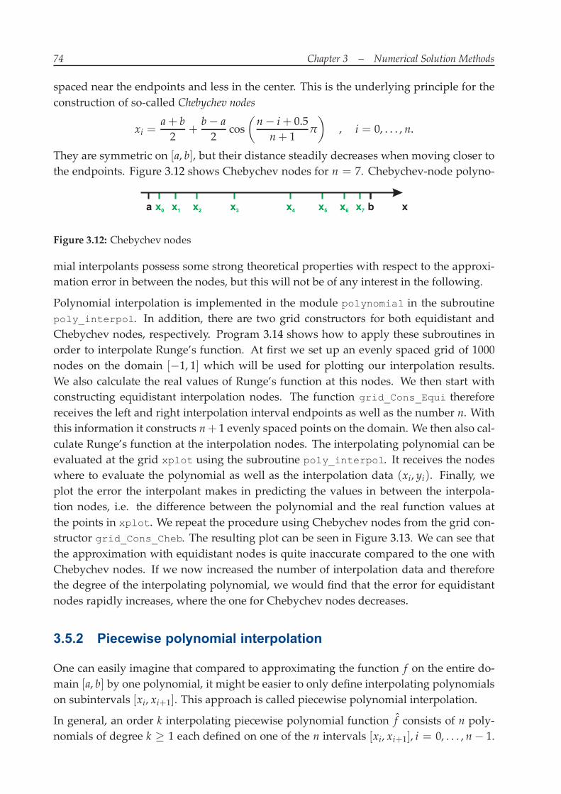
74 Chapter 3 – Numerical Solution Methods
spaced near the endpoints and less in the center. This is the underlying principle for theconstruction of so-called Chebychev nodes
xi =a+ b2
+b− a2
cos(n− i+ 0.5n+ 1
π
), i = 0, . . . , n.
They are symmetric on [a, b], but their distance steadily decreases when moving closer tothe endpoints. Figure 3.12 shows Chebychev nodes for n = 7. Chebychev-node polyno-
x0 x1 x2 x7x6x5x3 x4 xa b
Figure 3.12: Chebychev nodes
mial interpolants possess some strong theoretical properties with respect to the approxi-mation error in between the nodes, but this will not be of any interest in the following.
Polynomial interpolation is implemented in the module polynomial in the subroutinepoly_interpol. In addition, there are two grid constructors for both equidistant andChebychev nodes, respectively. Program 3.14 shows how to apply these subroutines inorder to interpolate Runge’s function. At first we set up an evenly spaced grid of 1000nodes on the domain [−1, 1] which will be used for plotting our interpolation results.We also calculate the real values of Runge’s function at this nodes. We then start withconstructing equidistant interpolation nodes. The function grid_Cons_Equi thereforereceives the left and right interpolation interval endpoints as well as the number n. Withthis information it constructs n+ 1 evenly spaced points on the domain. We then also cal-culate Runge’s function at the interpolation nodes. The interpolating polynomial can beevaluated at the grid xplot using the subroutine poly_interpol. It receives the nodeswhere to evaluate the polynomial as well as the interpolation data (xi, yi). Finally, weplot the error the interpolant makes in predicting the values in between the interpola-tion nodes, i.e. the difference between the polynomial and the real function values atthe points in xplot. We repeat the procedure using Chebychev nodes from the grid con-structor grid_Cons_Cheb. The resulting plot can be seen in Figure 3.13. We can see thatthe approximation with equidistant nodes is quite inaccurate compared to the one withChebychev nodes. If we now increased the number of interpolation data and thereforethe degree of the interpolating polynomial, we would find that the error for equidistantnodes rapidly increases, where the one for Chebychev nodes decreases.
3.5.2 Piecewise polynomial interpolation
One can easily imagine that compared to approximating the function f on the entire do-main [a, b] by one polynomial, it might be easier to only define interpolating polynomialson subintervals [xi, xi+1]. This approach is called piecewise polynomial interpolation.
In general, an order k interpolating piecewise polynomial function f̂ consists of n poly-nomials of degree k ≥ 1 each defined on one of the n intervals [xi, xi+1], i = 0, . . . , n− 1.

3.5. Function approximation and interpolation 75
Program 3.14: Polynomial interpolation of Runge’s function
program polynomials
! modulesuse polynomialuse ESPlot
! variable declarationimplicit noneinteger, parameter :: n = 10, nplot = 1000real*8 :: xi(0:n), yi(0:n)real*8 :: xplot(0:nplot), yplot(0:nplot), yreal(0:nplot)
! get equidistant plot nodesxplot = grid_Cons_Equi(-1d0, 1d0, nplot)yreal = 1d0/(1d0+25*xplot**2)
! equidistant polynomial interpolationxi = grid_Cons_Equi(-1d0, 1d0, n)yi = 1d0/(1d0+25*xi**2)yplot = poly_interpol(xplot, xi, yi)
! plot equidistant errorcall plot(xplot, yplot-yreal, ’Equidistant’)
! Chebychev polynomial interpolationxi = grid_Cons_Cheb(-1d0, 1d0, n)yi = 1d0/(1d0+25*xi**2)yplot = poly_interpol(xplot, xi, yi)
! plot equidistant errorcall plot(xplot, yplot-yreal, ’Chebychev’)
! execute plotcall execplot()
end program
It satisfies the interpolation conditions f̂ (xi) = f (xi) at the interpolation nodes and iscontinuous over the whole domain [a, b]. However, in opposite to an interpolating poly-nomial, an order-k piecewise polynomial function is only k − 1 times continuously dif-ferentiable on the whole interval [a, b], i.e. it is not as smooth as a polynomial. Notethat the problem of non-differentiability only arises at the interpolation nodes, where thepolynomial pieces are spliced together.
In the following we concentrate on two specific classes of piecewise polynomial inter-polants which are employed widely in practice. A first-order or piecewise linear functionis a series of line segments spliced together at the interpolation nodes to form a con-

76 Chapter 3 – Numerical Solution Methods
−1 −0.5 0 0.5 1
0
0.5
1
1.5
2
EquidistantChebychev
Figure 3.13: Equidistant vs. Chebychev nodes
tinuous function. A third-order function or cubic spline is a series of cubic polynomialsegments spliced together to form a twice continuously differentiable function. Figure3.14 compares piecewise linear f̂ LIN(x) and cubic spline f̂ SPL(x) interpolation for n = 4breakpoints.
x
f(x)
x0 x1 x2 x3
f (x)LIN^
f (x)SPL^
Figure 3.14: Piecewise linear interpolation vs. cubic splines
Piecewise linear functions are particularly easy to construct and evaluate in practice,which explains their widespread popularity. Assume an arbitrary set of interpolationdata (xi, f (xi)) to be given. In the interval [xi, xi+1] we define the approximating linearfunction fi as
f̂i(x) = c0,i + c1,ix,

3.5. Function approximation and interpolation 77
where the coefficients can be computed from the two interpolation conditions
f (xi) = c0,i + c1,ixif (xi+1) = c0,i + c1,ixi+1.
Assuming the nodes to be equidistant over the domain with h = b−an being the distance
between breakpoints, i.e. xi = a + ih, i = 0, . . . , n, the interpolating piecewise linearfunction is
f̂ (x) =(x− xi) f (xi+1) + (xi+1 − x) f (xi)
hif x ∈ [xi, xi+1].
Linear splines are attractive for their simplicity, however due to not being differentiableover the whole domain, they have some shortcomings which limit their application inmany computational economic problems. For example, when derivatives are required inorder to find extrema of a function usingNewton-likemethods, piecewise linear functionsare not a good choice. In such a case, cubic splines offer a better alternative. They retainmuch of the stability and flexibility of piecewise linear functions, but possess continuousfirst and second derivatives. Consequently, they typically produce adequate approxima-tions for both the function and its first and second derivatives.
The n− 1 piecewise third order polynomials of a cubic spline on the interval [xi, xi+1] are
f̂i(x) = c0,i + c1,ix+ c2,ix2 + c3,ix
3 , i = 0, . . . , n− 1.
Note that we now have 4n parameters to pin down our cubic spline. The required equa-tions are derived from the following conditions:
1. The polynomials have to replicate the function values at the interpolation nodes (2nequations)
c0,i + c1,ixi + c2,ix2i + c3,ix
3i = f (xi) , i = 0, . . . , n− 1,
c0,i + c1,ixi+1 + c2,ix2i+1 + c3,ix
3i+1 = f (xi+1) , i = 0, . . . , n− 1.
2. First derivatives of two consecutive polynomials at the inner interpolation nodeshave to be equal (n− 1 equations)
c1,i + 2c2,ixi + 3c3,ix2i = c1,i+1 + 2c2,i+1xi + 3c3,i+1x2i , i = 1, . . . , n− 1.
3. Second derivatives of two consecutive polynomials at the inner interpolation nodeshave to be equal (n− 1 equations)
2c2,i + 6c3,ixi = 2c2,i+1 + 6c3,i+1xi , i = 1, . . . , n− 1.
All in all thismakes 4n− 2 equations in order to compute 4n coefficients c0,i, c1,i, c2,i, c3,i, i =0, . . . , n − 1. The two missing equations can be derived in different ways. Typically

78 Chapter 3 – Numerical Solution Methods
one applies the condition for the so-called natural spline, which requires that the secondderivative is zero at the endpoints of the domain, i.e.
2c2,1 + 6c3,1x1 = 0
2c2,n + 6c3,nxn = 0.
This implies the spline function to be a straight line outside of the domain [a, b].
Technically, we could choose our interpolation nodes quite arbitrary on the domain. In-deed, the ability to distribute breakpoints unevenly over the domain adds considerablyto the flexibility of cubic splines, allowing them to accurately approximate a wide rangeof functions. However, there is a quite simple algorithm for computing the coefficientsof splines if interpolation nodes are equidistant. This algorithm is implemented in themodule spline. Piecewise linear interpolation with arbitrary interpolation nodes on theother hand is implemented in the module linint. Program 3.15 shows how to applyboth methods to Runge’s function. The use of those modules is pretty similar to the useof polynomial. The function linear performs a piecewise linear interpolation method.It receives exactly the same arguments as poly_interpol. The function spline howeverreceives the points where to evaluate the cubic spline function, the interpolation data yiand the left and right interval border of the interpolation domain. This is because theroutine already assumes the nodes xi to be equally spaced on the whole domain [a, b].We again plot the error terms for all our 1001 equally spaced nodes on [−1, 1]. Figure3.15 shows the results. Note that these module procedures are also able to handle multi-
−1 −0.5 0 0.5 1
−0.05
0
0.05
0.1
Piecewise linearCubic spline
Figure 3.15: Piecewise linear interpolation and cubic splines for Runge’s function
dimensional interpolation problems. However, this would go far beyond the scope ofthis chapter. Please refer to the module descriptions in the appendix on how to performmultidimensional interpolation.
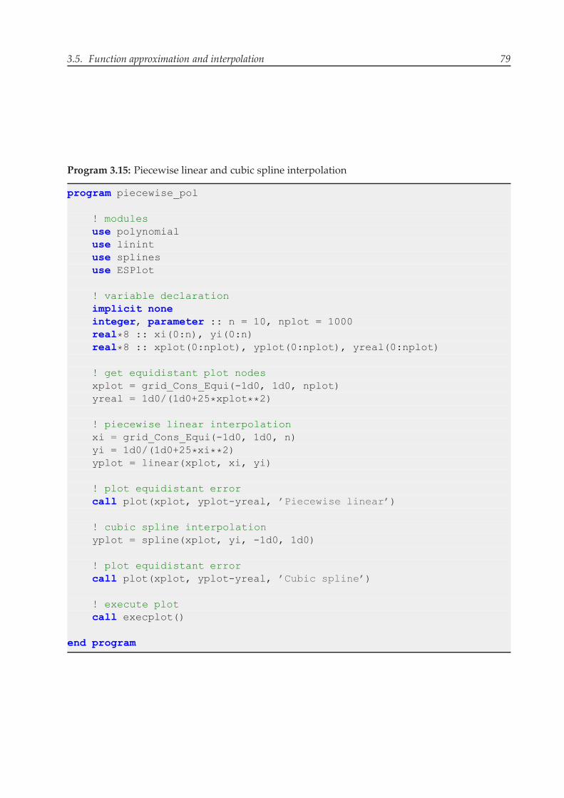
3.5. Function approximation and interpolation 79
Program 3.15: Piecewise linear and cubic spline interpolation
program piecewise_pol
! modulesuse polynomialuse linintuse splinesuse ESPlot
! variable declarationimplicit noneinteger, parameter :: n = 10, nplot = 1000real*8 :: xi(0:n), yi(0:n)real*8 :: xplot(0:nplot), yplot(0:nplot), yreal(0:nplot)
! get equidistant plot nodesxplot = grid_Cons_Equi(-1d0, 1d0, nplot)yreal = 1d0/(1d0+25*xplot**2)
! piecewise linear interpolationxi = grid_Cons_Equi(-1d0, 1d0, n)yi = 1d0/(1d0+25*xi**2)yplot = linear(xplot, xi, yi)
! plot equidistant errorcall plot(xplot, yplot-yreal, ’Piecewise linear’)
! cubic spline interpolationyplot = spline(xplot, yi, -1d0, 1d0)
! plot equidistant errorcall plot(xplot, yplot-yreal, ’Cubic spline’)
! execute plotcall execplot()
end program

80 Chapter 3 – Numerical Solution Methods
3.6 Linear programs
In planning production processes and in several logistic problems one usually finds one-self confronted with solving a linear program. A linear program in standard form is givenby the optimization problem
minx1,...,xn
c1x1 + c2x2 + . . .+ cnxn with xi ≥ 0 , i = 1, . . . , n
with the m inequality constraints
a11x1 + a12x2 + . . .+ a1nxn ≤ b1a21x1 + a22x2 + . . .+ a2nxn ≤ b1
...
am1x1 + am2x2 + . . .+ amnxn ≤ bm.With the matrices and vectors
A =
⎡⎢⎢⎢⎢⎣a11 a12 . . . a1na21 a22 . . . a2n...
... . . . ...am1 am2 . . . amn
⎤⎥⎥⎥⎥⎦ , b =
⎡⎢⎢⎢⎢⎣b1b2...bm
⎤⎥⎥⎥⎥⎦ , c =
⎡⎢⎢⎢⎢⎣c1c2...cn
⎤⎥⎥⎥⎥⎦ and x =
⎡⎢⎢⎢⎢⎣x1x2...xn
⎤⎥⎥⎥⎥⎦ ,
we can write
minxcTx s.t x ≥ 0 and Ax ≤ b.
Example Consider a company that produces two goods x1 and x2 on one type of ma-chine. Due to storage capacity, the production is limited to 100 pieces altogether. Theproduction of the two goods requires time and raw material. Good 1 thereby is a timeand cost intensive production good which requires 4 hours of production time and rawmaterial worth 20 Euros per piece. Good 2 is less intensive and can therefore be producedwithin 1 hour and with raw material worth 10 Euro. The company owns 8 machineswhich can run 20 hours a day. The remaining time has to be spent on maintenance. Inaddition, overall costs of raw material should be limited to 1100 Euro per day. The twogoods can be sold on the market for the prices 120 and 40 Euros, respectively. What is theoptimal production of goods per day for the company?
Table 3.1 summarizes the problem. The goal of the company obviously is to maximizeits profits 120x1 + 40x2 subjects to the given production constraints. This problem can bewritten as a linear program in standard form
minx1,x2
−120x1 − 40x2 , x1, x2 ≥ 0
subject to the constraints
x1 + x2 ≤ 100

3.6. Linear programs 81
4x1 + x2 ≤ 160
20x1 + 10x2 ≤ 1100.
Note that we again just minimize the negative of the objective function in order to maxi-mize it. The same approach was chosen in the section that dealt with the minimization ofnon-linear functions.
Type 1 Type 2 Restriction
Pieces per day 1 1 100Time input 4 1 160Raw material 20 10 1100
Market price 120 40 ?
Table 3.1: Linear programming example
3.6.1 Graphical solution to linear programs in standard form
There is an intuitive graphical solution method to linear programs in standards form.Figure 3.16 shows how this solution looks like. We first have to draw the three inequality
x1
x2
160
110
100
40 55 100
60
25 x1
x2
160
110
100
40 55 100
Π = 2400
Π = 5400
Figure 3.16: Graphical solution to linear programs in standard form
constraints. All x1-x2 combinations that satisfy such a constraint lie below the line onwhich equality holds. In our example, these equality lines can be computed as
x2 = 100− x1

82 Chapter 3 – Numerical Solution Methods
x2 = 160− 4x1x2 = 110− 2x1.
These lines are depicted as black, green and blue line in the left part of the figure, respec-tively. The area, in which all of the three inequalities hold simultaneously, i.e. where x1and x2 lie below all of the three lines simultaneously, is the gray shaded area. Note thatalso x1, x2 ≥ 0 has to hold. The gray shaded area therefore represents our feasible set ofx1-x2 combinations.
Next, we look at the iso-profit lines of the company. An iso-profit line is the set of all x1-x2combinations leading to the same profit Π, i.e.
x2 =Π40
− 3x1.
The iso-profit line for Π = 2400 is the red line in the right part of Figure 3.16. The morethe line is on the right, i.e. the higher the y-intercept, the higher are the company’s profits.We therefore take the iso-profit line and make a parallel shift to the right. We can do thisup to the point where we touch the border of our feasible solution set. The point markedin red, where the iso-profit line exactly touches this set then is our optimal solution, as itguarantees the highest profit, given that x1 and x2 satisfy the three inequality conditions.Note that our optimum is defined by the intersection point between the green and theblue line, i.e. constraints two and three hold with equality. We therefore can compute ouroptimum via calculating the intersection point between the two equality lines, i.e. setting
160− 4x1 = 110− 2x1⇒ x∗1 = 25 and x∗2 = 60.
Note that, due to x∗1 + x∗2 = 85 < 100, constraint one is not binding. The maximum profit
the company makes finally is
Π∗ = 120x∗1 + 40x∗2 = 5400.
3.6.2 The simplex algorithm
The graphical solution to a linear program is quite intuitive and easy to handle, if theprogram is given in standard form and there are only two choice variables. However,in practice, the number of variables and constraints usually is quite high. In addition,beneath inequality constraints, we could also have equality constraints in our program.We therefore define the canonical form of a linear program as
minxcTx s.t x ≥ 0 and Ax = b.
There is a quite efficient and often used algorithm for solving linear programs in canonicalform called the simplex algorithm invented by George Danzig in 1947. The idea behind this
3.6. Linear programs 83
algorithm is as follows: From the above figure we can already guess that the solution toa linear program must be a so-called corner of the set of feasible solutions. Corners, inthe above problem, are points where two equality lines (including the axes) intersect. Thesimplex algorithm therefore basically checks all corners of the set of feasible solutions andchooses the corner point that minimizes the objective function.
The problem with the simplex algorithm is that it only applies to linear programs incanonical form, not in standard form. In general, however, linear programs will not onlyconsist of equality constraints. Nevertheless, any linear program with inequality con-straints can be turned into a canonical form problem via the following transformation:Assume the general linear program
minx1,...,xn
c1x1 + c2x2 + . . .+ cnxn
with the set of constraints
a11x1 + a12x2 + . . . + a1nxn ≤ b1...
ak1x1 + ak2x2 + . . . + aknxn ≤ bkak+1,1x1 + ak+1,2x2 + . . . + ak+1,nxn = bk+1
am1x1 + am2x2 + . . . + amnxn = bm
with k inequality constraints. For simplicity we’ve dropped out greater-than-or-equalityconstraints. Note, however, that we can turn any of those constraints into a lower-than-or-equality constraint by just multiplying the whole constraint with −1. In the abovelinear program, we can now introduce so-called slack variables y1, y2, . . . , yk ≥ 0. If wereformulate the program as
minx1,...,xn,y1,...,yk
c1x1 + c2x2 + . . .+ cnxn
with
a11x1 + a12x2 + . . . + a1nxn + y1 = b1...
ak1x1 + ak2x2 + . . . + aknxn + yk = bkak+1,1x1 + ak+1,2x2 + . . . + ak+1,nxn = bk+1
am1x1 + am2x2 + . . . + amnxn = bm
we obtain a linear program in canonical form to which we can apply the simplex al-gorithm. Note that the slack variables do not change the objective function. If a slackvariable yi in the optimum is strictly greater than zero, this indicates that the respectiveconstraint is not binding, like constraint one in the above example.
The simplex algorithm is implemented in subroutine linear_sol in themodule simplex.Program 3.16 demonstrate how to use it. First we have to define the parameters of the lin-ear program. The constraints are represented by amatrix A and a vector b as shown above.
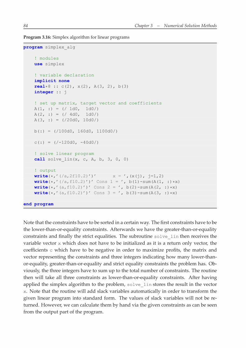
84 Chapter 3 – Numerical Solution Methods
Program 3.16: Simplex algorithm for linear programs
program simplex_alg
! modulesuse simplex
! variable declarationimplicit nonereal*8 :: c(2), x(2), A(3, 2), b(3)integer :: j
! set up matrix, target vector and coefficientsA(1, :) = (/ 1d0, 1d0/)A(2, :) = (/ 4d0, 1d0/)A(3, :) = (/20d0, 10d0/)
b(:) = (/100d0, 160d0, 1100d0/)
c(:) = (/-120d0, -40d0/)
! solve linear programcall solve_lin(x, c, A, b, 3, 0, 0)
! outputwrite(*,’(/a,2f10.2)’)’ x = ’,(x(j), j=1,2)write(*,’(/a,f10.2)’)’ Cons 1 = ’, b(1)-sum(A(1, :)*x)write(*,’(a,f10.2)’)’ Cons 2 = ’, b(2)-sum(A(2, :)*x)write(*,’(a,f10.2)’)’ Cons 3 = ’, b(3)-sum(A(3, :)*x)
end program
Note that the constraints have to be sorted in a certain way. The first constraints have to bethe lower-than-or-equality constraints. Afterwards we have the greater-than-or-equalityconstraints and finally the strict equalities. The subroutine solve_lin then receives thevariable vector x which does not have to be initialized as it is a return only vector, thecoefficients c which have to be negative in order to maximize profits, the matrix andvector representing the constraints and three integers indicating how many lower-than-or-equality, greater-than-or-equality and strict equality constraints the problem has. Ob-viously, the three integers have to sum up to the total number of constraints. The routinethen will take all three constraints as lower-than-or-equality constraints. After havingapplied the simplex algorithm to the problem, solve_lin stores the result in the vectorx. Note that the routine will add slack variables automatically in order to transform thegiven linear program into standard form. The values of slack variables will not be re-turned. However, we can calculate them by hand via the given constraints as can be seenfrom the output part of the program.