Numerical Solution for Eigenvalues and Eigenfunctions of a ...the eigenvalues pkn, k = 1, . . . ,...

MATHEMATICS OF COMPUTATION, VOLUME 29, NUMBER 131

JULY 1975, PAGES 794-805

Numerical Solution for Eigenvalues

and Eigenfunctions of a Herrn i t i a n Kernel

and an Error Estimate

By E. Rakotch

Abstract. New error estimates for eigenvalues of symmetric integral equations are ob-

tained. These estimates are applicable to a more general class of integration methods

and, in many cases, are better than those of Wielandt. For every eigenvalue, a numeri-

cal solution for the corresponding eigenfunction is also obtained. Whenever the exact

eigenvalue happens to be simple, an error estimate for the corresponding eigenfunction

is alsg derived.

1. Introduction. Let K(x, t) be a Hermitian kernel defined in / x /, where / =

[a, b], i.e., K(t, x) = K(x, t), such that

F(x) = f lA:(x, t)\2 dt is bounded in /;J a

then all the characteristic values p¡ of K(x, t) axe real and there exists an orthonormal

set {y¡(x)} of characteristic functions [5], i.e.,

(1) f*K(x, t)y¡(t) dt = Piyt(x), (y¡, y¡) = 8ijt

where (m, v) = f£u(x)v(x)dx is the scalar product of two complex functions m(x),

v(x)EL2(I)={z(x)\(z, z)<°°}.

Further, let S be a rule of numerical integration with weights win > 0 and nodes

xinEI, 7=1,...,«, by which the approximation /*f(x) dx "•» 2"=1 winf(xin) is

made.

To obtain a numerical solution for the characteristic values of K(x, t), Wielandt

[9] replaced the original problem by the sequence of eigenproblems

(2) K^y^=piny¡"\ K^ = wjnK(xtn,xjn), i,j=l,...,n,

with real pin and 77 linearly independent eigenvectors y\n^, for a class of integration

rules possessing the properties

lim Z winf(xin) = (bf(x)dx for every f(x) E C(I),

(3) Z"in = b-a;1=1

the eigenvalues pkn, k = 1, . . . , 71, are then taken by Wielandt as approximations,

which also converge as ti —► °°, to the corresponding characteristic values of K(x, t).

To specify this correspondence, the following assumptions are made:

Received July 2, 1972; revised December 2, 1974.

AMS (MOS) subject classifications (1970). Primary 65R05.Copyright © 1975, American Malhemariral Society

794

License or copyright restrictions may apply to redistribution; see https://www.ams.org/journal-terms-of-use

NUMERICAL SOLUTION AND AN ERROR ESTIMATE 795

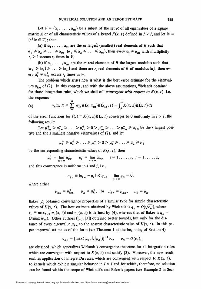
Let V = {a., . . . , am} be a subset of the set R of all eigenvalues of a square

matrix A or of all characteristic values of a kernel F(x, t) defined in / x /, and let W =

{z2\zE F};then

(a) if a., . . . , am axe the 772 largest (smallest) real elements of R such that

a1>ct2> . . .>otm (a. < a2 < . . . < am), then every a¡ =?-= am with multiplicity

rt > 1 occurs r¡ times in V,

(b) if a., . . . , am axe the ttj real elements of R the largest modulus such that

IctjI > lo£21 > . . . > \am\ and there are r¡ real elements of R of modulus la,-!, then ev-

ery a? -# a2m occurs r¡ times in W.

The problem which arises now is what is the best error estimate for the eigenval-

ues pkn of (2). In this context, and with the above assumptions, Wielandt obtained

for those integration rules, which we shall call convergent with respect to K(x, t)—i.e.

the sequencen b

(4) r?„(x, t) = Z winK(x, xin)K(xin, t) - J tf(x, z)K(z, t)dzi=l a

of the error functions for f(z) = K(x, z)K(z, t) converges to 0 uniformly in / x /, the

following result:

■Let tin > tin > ■ ■ • > Prn > 0 > fÇn > * * * > ^2» > ^in be the r largest posi-

tive and the s smallest negative eigenvalues of (2), and let

pt > p+ > . . .> pt > 0> p- > . . .> p2> P\

be the corresponding characteristic values of K(x, t); then

p.* = Urn pfn, pj = lim pjn, i = 1, . . . , r, j = 1, . . . , s,

and this convergence is uniform in i and/, i.e.,

where either

Pkn = tin' Mfc = Mfc, or Pkn=pkn, Pk=Pk.

Baker [2] obtained convergence properties of a similar type for simple characteristic

values of K(x, t). The best estimate obtained by Wielandt is qn = Oirsfe^), where

en = max/x/lT?„(x, i)l and r)„(x, t) is defined by (4), whereas that of Baker is qn =

0(max win). Other authors ([1], [3]) obtained better bounds, but only for the dis-

tance of every eigenvalue pkn to the nearest characteristic value of K(x, t). In this pa-

per improved estimates of the form (see Theorem 1 at the beginning of Section 4)

okn = [max(l/ifcfJl, \pk\)]-xpn, pn = 0(e„),

are obtained, which generalizes Wielandt's convergence theorems for all integration rules

which are convergent with respect to K(x, t) and satisfy (3). Moreover, the new result

enables application of integraticm rules, which are convergent with respect to K(x, t),

to kernels which exhibit singular behavior in / x / and for which, therefore, no solution

can be found within the scope of Wielandt's and Baker's papers (see Example 2 in Sec-


796 E. RAKOTCH

tion 2). As a consequence, an error estimate for the numerical solution of (1), conver-

gent to 0 uniformly in / for every integration rule which is convergent with respect to

K(x, t), is derived. The new error estimates for eigenvalues are to be interpreted as

follows: our estimates are better than those of Wielandt for the first mn eigenvalues

pkn such that max(ljUfc„l, \pk\) > C\Je~^ for some C> 0, where the sequence mn tends

to infinity; for other eigenvalues both our and Wielandt's estimates are of the same or-

der of magnitude, namely 0(\fe~^), and ours are not necessarily better.

2. Numerical Results. To illustrate the superiority of the new error estimates giv-

en by Theorem 1 in Section 4, two numerical examples are presented. To the second

of our examples Wielandt's method does not apply.

In the tables of results given below, pfn and pjn axe the eigenvalues defined in

Theorem 2 near the end of Section 4, whereas .^(x) and yjn(x) are the numerical so-

lutions for characteristic functions corresponding to pfn and p~~n, respectively, obtained

by the procedure described at the end of Section 4. The improved error estimates are

those described in Section 5. The error estimates for ^^(x) and yjn(x) axe those ob-

tained by application of the remark concluding the discussion of Theorem 3 in Section 4.

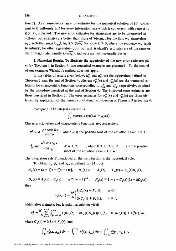
Example 1. The integral equation is

jQ max(x, t)y(t) dt = py(x).

Characteristic values and characteristic functions are, respectively:

R2 and —-r—r—, where R is the positive root of the equation z tanh z = 1 ;coshÄ

\¡2 cos rNx-rN and-, N = 1,2,..., where 0 < r. < r2 < . . . axe the positive

cos r*jroots of the equation z tan z 4 l = 0.

The integration rule 5 mentioned at the introduction is the trapezoidal rule.

To obtain an, ßn and yn, as defined in (24), put

An(z) = (n- l)z - [in - l)z], Bniz) = 1 - An(z), Cniz) = Aniz)Bniz),

Dn(z) = An(z) - Bn(z), h = (n- l)~x, Fn(z) = 1 - z - C„(z)[3z - hD„(z)];

then

h2 (3tCn(x) 4 Fn(t), x<t,

T? (X, t) = -7-\

6 l3xCn(t) 4 Fn(x), x>t,

which after a simple, but lengthy, calculation yields

.4 n-1 kn

< - Ig E .)(*_!)„'W) + hC„(t)Dn(t)[Gn(t) 4 0.3tCn(t)] 4 F2(t)}dt,

where Gn(t) = 0.3t 4 Fn(t), and

J0 »£(*. xin)dx = f '" n2n(x, xin)dx 4 C n2n(x, xin)dx." J xin



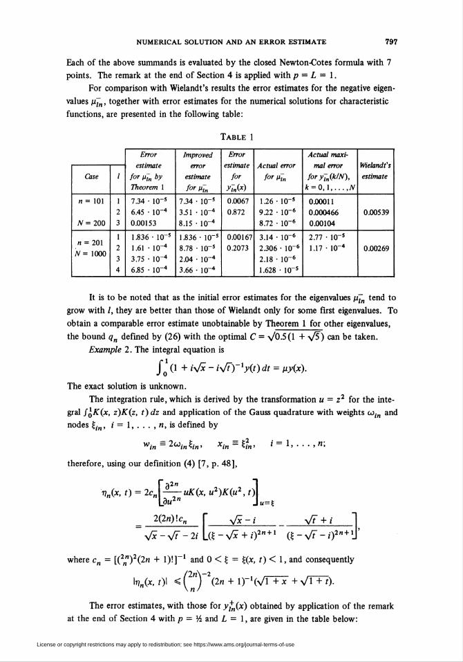
Each of the above summands is evaluated by the closed Newton-Cotes formula with 7

points. The remark at the end of Section 4 is applied with p = L = 1.

For comparison with Wielandt's results the error estimates for the negative eigen-

values pjn, together with error estimates for the numerical solutions for characteristic

functions, are presented in the following table:

Table 1

(Lase

Error

estimate

for p.~n by

Theorem 1

Improved

error

estimate

f°r »In

Error

estimate

for

yJn(*)

Actual error

Actual maxi-

mal error

foryJnik/N),

k = 0,1.N

Wielandt's

estimate

n= 101

#=200

7.34 - 10_s

6.45 • 10"4

0.00153

7.34

3.51

8.15

IO-5

io"4

io-4

0.0067

0.872

1.26- 10"5

9.22 • 10-6

8.72 • IO"6

0.00011

0.000466

0.00104

0.00539

n = 201

N= 1000

1.836 • 10-s

1.61 - 10"4

3.75 • 10"4

6.85 - 10"4

1.836 • 10"s

8.78 • IO-5

2.04 ■ 10"4

3.66 - 10"4

0.00167

0.2073

3.14 • IO"6

2.306 • IO"6

2.18 • 10"61.628 • 10"s

2.77

1.17

IO"5

IO"4 0.00269

It is to be noted that as the initial error estimates for the eigenvalues pjn tend to

grow with /, they are better than those of Wielandt only for some first eigenvalues. To

obtain a comparable error estimate unobtainable by Theorem 1 for other eigenvalues,

the bound qn defined by (26) with the optimal C = \J0.5il + \ß) can be taken.

Example 2. The integral equation is

J*o! (1 + z\£ - isjtyxy(t) dt = py(x).

The exact solution is unknown.

The integration rule, which is derived by the transformation u = z2 for the inte-

gral JqK(x, z)Kiz, t) dz and application of the Gauss quadrature with weights co/n and

nodes %in, i = 1, . . . , n, is defined by

win = 2">in tin > Xin " & > * " * ' n;

therefore, using our definition (4) [7, p. 48],

nn(x, t) = 2cn\^-uK(x, u2)K(u2, t)\La«2" J«=£

-\/F-2/b-v£ + 02" + 1

2(27

v*7

y/T 4 j

(?-VT-02"+1J

where cn = [(2„")2(2n + l)!]"1 and 0 < | = £(x, t) < 1, and consequently

kn(x, t)\ <Çn)2(2n 4 l)-x(y/TTx~ 4 vTTT).

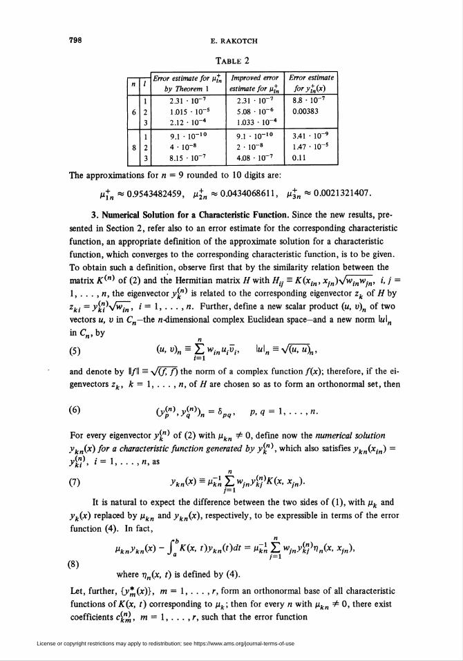
The error estimates, with those for yfn(x) obtained by application of the remark

at the end of Section 4 with p = \h and L — 1, are given in the table below:


798 E. RAKOTCH

Table 2

Error estimate for pfn

by Theorem 1

2.31 • IO"7

1.015 ■ IO"5

2.12 • IO"4

9.1 ■ IO"10

4 • 10"8

8.15 * IO"7

Improved error

estimate for pfn

2.31 ■ IO"7

5.08 • 10~6

1.033 • IO"4

9.1 • 10"10

2 • IO"8

4.08 • IO"7

Error estimate

fory^jx)

8.8 • IO"7

0.00383

3.41 • IO"91.47 ■ 10"s

0.11

The approximations for 77 = 9 rounded to 10 digits are:

p+n « 0.9543482459, /ti+i « 0.0434068611, p+n * 0.0021321407.

3. Numerical Solution for a Characteristic Function. Since the new results, pre-

sented in Section 2, refer also to an error estimate for the corresponding characteristic

function, an appropriate definition of the approximate solution for a characteristic

function, which converges to the corresponding characteristic function, is to be given.

To obtain such a definition, observe first that by the similarity relation between the

matrix A"(n) of (2) and the Hermitian matrix H with Hif = K(xin, x1n)yjwtnwjn, i, j =

1, . . . , 77, the eigenvector yk"^ is related to the corresponding eigenvector zk of H by

zki = yíl vwin - i = 1, ■ ■ ■ ,n- Further, define a new scalar product (m, v)n of two

vectors u, v in Cn— the 77-dimensional complex Euclidean space—and a new norm Iwl^

inC„,byn

(5) (". v)n - £ winuiV¡> ]uln ~ V(«, ")„,f=l

and denote by 11/11 = \f(J, f) the norm of a complex function fix); therefore, if the ei-

genvectors zk, k = 1, . . . , n, of H are chosen so as to form an orthonormal set, then

(6) (v(n) v(n)\ _ §vp ' Xq )n upq ■ p, q = 1, . . . ,n.

For every eigenvector ykn) of (2) with pkn ¥= 0, define now the numerical solution

ykn(x) for a characteristic function generated by ykn), which also satisfies ykn(xin) -

ykn), i = 1, ... ,7î, as

(V) ykn(x) = pkxn Z V§>K(x, xjn).7=1

It is natural to expect the difference between the two sides of (1), with pk and

yk(x) replaced by pkn and ykn(x), respectively, to be expressible in terms of the error

function (4). In fact,

Pknykn(x) - Jfl K(x, t)ykn(t)dt = pkxn Z winy{kfr}n(x, xjn),

(8)where vn(x, t) is defined by (4).

Let, further, {j** (x)}, m = I, . . . ,r, form an orthonormal base of all characteristic

functions of ^(x, t) corresponding to pk; then for every 77 with pkn ^ 0, there exist

coefficients ck"J,, m = 1, . . . , r, such that the error function



r

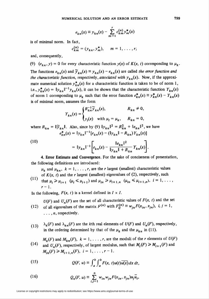
ek„{x)=ykH(x)- Z cknmym(x)m = l

is of minimal norm. In fact,

Lkm \ykn->^m{n)=(ykn^m)> m=\,...,r,

and, consequently,

(9) (ekn,y) = 0 for every characteristic functiony(x) of K(x, t) corresponding to pk.

The functions ekn(x) and ^„(x) = ykn(x) - ekn(x) axe called the error function and

the characteristic function, respectively, associated with ykn(x). Now, if the approxi-

mate numerical solution ykn(x) for a characteristic function is taken to be of norm 1,

i.e.,ykn(x) = Wykn\\~lykn(x), it can be shown that the characteristic function Ykn(x)

of norm 1 corresponding to pk such that the error function e*n(x) = .y*„(x) - ^„(x)

is of minimal norm, assumes the form

ÍRknykn(x), Rkn * 0>

\y¡(x) with pt = pk, Rkn = °>

where Rkn = \\yknW. Also, since by (9) Wykn\\2 = R2kn 4 lekn\\2, we have

4n(*> = I^JI_1K„(x) - (\\ykJ-Rkn)Ykn(x)]

(10) lleknll2 "1

4. Error Estimate and Convergence. For the sake of conciseness of presentation,

the following definitions are introduced:

pk and pkn, k = 1, . . . , r, are the r largest (smallest) characteristic values

of K(x, t) and the r largest (smallest) eigenvalues of (2), respectively, such

that pt > pi+l (Pi < pi+1) and pin > pi+ln (pin < Pl+lt„), i - 1, ... ,

r- 1.

In the following, ^(x, t) is a kernel defined in / x /.

U(F) and Un(F) axe the set of all characteristic values of F(x, t) and the set

(12) of all eigenvalues of the matrix F(n) with f£*> = wjnF(xin, xjn), i, / = 1,

... ,77, respectively.

(13) *V(^) an(l \n(F) are tne *tn real elements of C/(F) and Un(F), respectively,

in the ordering determined by that of the pk and the pkn in (11).

Mk(F) and Mkn(F), k = 1.r, are the moduli of the r elements of U(F)

(14) and Un(F), respectively, of largest modulus, such that M¡(F) > Mi+.(F) and

Min(F)>Mi+ln(F), i=l,...,r-l.

<15) Q(F, u) = fb (bF(x, t)u(t)ujx)dx dt,J a J a

n

(16) Q„(F,U)= Z winwjnF(xin> xjn)ujui>i,j=l


800

(17)

(18)

(19)

(20)

(21)

E. RAKOTCH

(24)

(25)

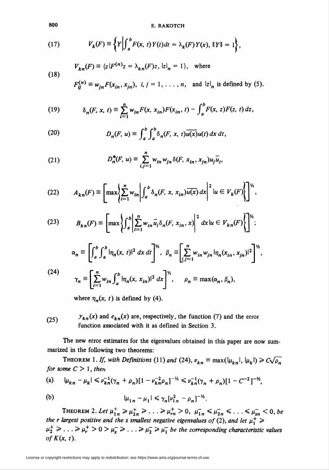
Vk(F) = |r|j^(x, t)Y(t)dt = $F)Y(x), WYW = l|,

Vkn(F) = {z\F^z = Xkn(F)z, \z\n = 1}, where

rff* - wjnF(xin>xjn)> i, / = 1, • • • , «, and lzl„ is defined by (5).

on(F, x,t) = Z winF(x, xin)F(xin, t) - fbF(x, z)F(z, t)dz,i=i

Dn(F, u) = /*/"«„(F, *> t)u(x)u(f)dxdt,

Dn°(F> ")= Z winwjnd(F> Xin<Xjn)Ujui>Í.7-1

(22) ¿fe„(F) = ímaxj¿ w,.„ £ 8n(F, x, xin)u(x)dx * Im G Fk(F)jj ,

dxlMGKk„(F) j ;(23) 5 „(F) = max \\ \Z win «,• 5„(F, x,„,.L ( l'=1

a"~ \faialV"(X't)l2dXdt\ ' ß"~\£.WinWjMXin'Xjn)l2\ >

r " fb T/:T„ S EWm Ja It-«(*> */«)12 dx P„ =max(a„,ß„),

where rj„(x, t) is defined by (4).

ykn(x) and ekn(x) are, respectively, the function (7) and the error

function associated with it as defined in Section 3.

The new error estimates for the eigenvalues obtained in this paper are now sum-

marized in the following two theorems:

Theorem I. If, with Definitions (11) and (24), vkn = max(\pkn\, \pk$ > C\[p^

for some C > 1, then

(a) \pkn - pk\ < v-kniyn 4 pn)[l - vk2npn]-* < ^(T„ + p„)[l - C"2]-*,

(b) ^1«-^I<7„K2„-P„r1/2.

Theorem 2. Let p+n > p+n > . . . > p?n > 0, p~n < p2n < . . . < pjn < 0, be

the r largest positive and the s smallest negative eigenvalues of (2), and let p+ >

p2 > . . . > p, > 0 > pj > . . . > p2 > p[ be the corresponding characteristic values

ofKix, t).



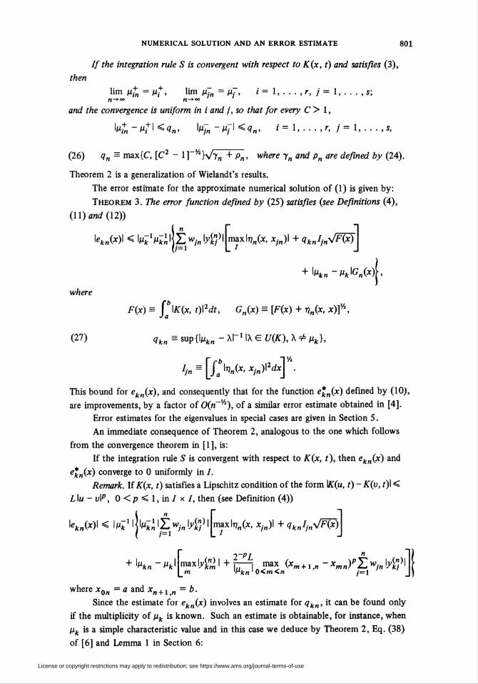
// the integration rule S is convergent with respect to K(x, t) and satisfies (3),

then

it =u+,in r^l '

and the convergence is uniform in i and j, so that for every C> 1,

lim pfn = pt, lim pjn = pf, i = 1.r, j = 1.s;

Wn ~ti^ <(?«' ^jn ~Pj ' <-?»- i = 1, . . . ,r, /= 1, . . . ,s,

(26) <?„ = max{C, [C2 - 1] V2Wyn 4 pn, where y„ and pn are defined by (24).

Theorem 2 is a generalization of Wielandt's results.

The error estimate for the approximate numerical solution of (1) is given by:

Theorem 3. The error function defined by (25) satisfies (see Definitions (4),

(ll)ú*77<Í(12))

lek„(x)l < l/ifcVkiKÉw/J.)>k/)l maxLí?„(x, x/n)l + qknIjns/Flx)\\i=i L I J

4\pkn -pk\Gnix)\,

where

Fix) = \b\K(x, t)\2dt, Gn(x) = [F(x) + t?„(x, x)f,

(27) qkn = sup{ljuk„ - \\~x IX E U(K), X * pk},

Ijn-\Jalr,^X'Xi^l2dX\ ■

This bound for ekn(x), and consequently that for the function ekn(x) defined by (10),

are improvements, by a factor of 0(7i_y2), of a similar error estimate obtained in [4].

Error estimates for the eigenvalues in special cases are given in Section 5.

An immediate consequence of Theorem 2, analogous to the one which follows

from the convergence theorem in [1], is:

If the integration rule 5 is convergent with respect to K(x, t), then ek„(x) and

ekn(x) converge to 0 uniformly in I.

Remark. If K(x, t) satisfies a Lipschitz condition of the form IK(m, t)-K(v, t)\ <

L\u - v\p, 0 <p <l,inl x I, then (see Definition (4))

■«*„{*)! < I M* * IJ lMfc¿ l¿ w/n bg> I |n»x Itï„(*. xjn)\4qknIins/mj

I2"PL " ]maxlyfc"„> I + r—i max (xm +, —- xmn)PZ wjn \ykf\m 'Pkn' 0<m<n /=l J]

where x0„ =aandx„ + 1„ = b.

Since the estimate for ekn(x) involves an estimate for qkn, it can be found only

if the multiplicity of pk is known. Such an estimate is obtainable, for instance, when

pk is a simple characteristic value and in this case we deduce by Theorem 2, Eq. (38)

of [6] and Lemma 1 in Section 6:


802 E. RAKOTCH

Corollary 1. If pk is a simple characteristic value of Kix, t) and the integra-

tion rule is convergent with respect to K(x, t) and satisfies (3), then for some choice

of eigenvectors ykn^ such that lyk"\ = 1 (see Definitions (5) and (7)),

ykn(x) ~* yk(x) uniformly in I, and so does also WyknW~lykn(x).

By (7) it follows that

ibfe„ii2 »n*2 Z ^n^jny¥)ykni)G(xin,xjn)U=l

where

G(x, t) = (bK(z, x)K(z, t)dz = ¡bK(x, z)K(z, t)dz.J a Ja

In the case where G(x, t) cannot be determined exactly, an approximation ckn

of H.yknll is found by applying some quadrature formula for determining G(x, t) at the

points (xin, x-n); the approximate solution for a characteristic function is then taken

to be ckxykn(x), and the error estimate is

2*„0O - Ü;iykHQc)-R-ki\ykn(x)\ < \(ck„ - Wykn\\-l)ykn(x)\ + Kn(x)\

= (cknhkJTl\(ckn - *ykJ)yk„(x)\ 4 \e*kn(x)\,

where e*n(x) is given by (10).

5. Improved Error Estimates for Simple Characteristic Values and for Positive-

Definite Kernels. An error estimate for a simple characteristic value can be improved if

the approximate eigenvalue pkn satisfies the inequality (see Definition (11))

Kn -/**■< "i11 *M*„ -M;!-i¥=k

If the integration rule 5 is convergent with respect to K(x, t) and satisfies (3),

and pk is a simple characteristic value, then by Theorem 2 there exists an integer N

such that the above inequality holds for n> N, and by Lemma 5 (stated in Section 6)

\pkn~Pk\ = inffX„ -XI IX G U(K)} < \pilH\iykJ-%.

An error estimate for a positive-definite kernel is obtained from the following

theorem:

Theorem 4. Let pkn E Un(K) and pk E U(K), k = l,...,n, such that

fr*«1 = Mkn(K) and \pk\ = Mk(K) (see Definitions (12), (14) and (4)). 777C77

ÇÎ2„ -p2\ <Ml(nn) 4 Mln(nn), k=l,2,...,

where pkn = 0 for k> n.

Corollary 2. If K(x, t) is positive-definite and (see Definitions (11) and (12)),

pkn > -min{XlX G Un(K)}, then, \p\n - p\\ <M1(t?„) + Mlninn).

We also obtain

Corollary 3. Ií¿„+kl <\jMxit,n), k = 1,2, . . . .

6. Discussion of the Theorems. To obtain the final results presented in Theorems

1-4, the following lemmas are necessary using the definitions introduced at the begin-

ning of Section 4:



Lemma 1. Let un= (unl,. . . , unn) and An = (fl,-,"-1) be, respectively, sequences

of vectors and n x n matrices with complex elements. Then (see Definition (5))

(a) Im„I2 = S«=, I(m„, zk)„l2 = 2g=, I(zk, m„)„I2 for every sequence zk, k =

1, . . . , 7i, satisfying

(28) (Zp>Zq)n = dpq> P. Í - 1, . . . , H.

(b) If the integration rule S satisfies (3), then

n n

lim maxlMnil = 0 implies lim Z winuni = um £ win Mfc/*Mní' = 0>n-*°° i n-*°°i=x n-*°°i=x

k = l,2,...,

andn

lim maxlflj^l = 0 implies lim Z winwjnaí¡'^ = °*n-*"" í.7 »-+<"• í,/*-=l

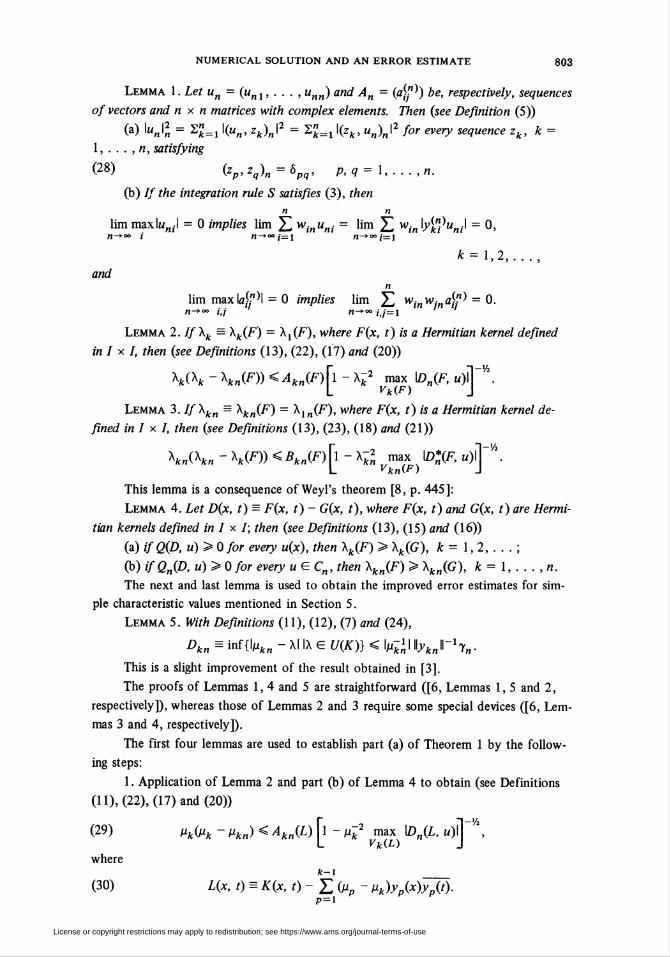
Lemma 2. // Xk = Xk(F) = X,(F), wfcere F(x, í) is a Hermitian kernel defined

in I x I, then (see Definitions (13), (22), (17) and (20))

Xk(Xk - Xkn(F))<Akn(F)\l - Xk2 max lD„(F, u)\]~V\I VkiF) J

Lemma 3. If Xkn = Xkn(F) = X,„(F), w/7e7*e F(x, i) is a Hermitian kernel de-

fined in I x I, then (see Definitions (13), (23), (18) and (21))

X*„(X*„ - Xk(F)) <Bkn(F)\l - Xk2 max \D*(F. u)\[V\L VkniF) J

This lemma is a consequence of Weyl's theorem [8, p. 445]:

Lemma 4. Let Dix, t) = F(x, t) - G(x, ¿)> vv7ze7*e F(x, /) an<i G(x, i) are Hermi-

tian kernels defined in I x I; then (see Definitions (13), (15) and (16))

(a) if Q(D, u)>0 for every u(x), then Xk(F) > Xk(G), k= 1,2,...;

(b) if Qn(D, u)>0 for every u E Cn, then \kn(F) > \n(G), k=l_77.

The next and last lemma is used to obtain the improved error estimates for sim-

ple characteristic values mentioned in Section 5.

Lemma 5. With Definitions (11), (12), (7) and (24),

Dkn = inf{\pkn -XIIXg U(K)} < \p-knW\ykn\\-xyn.

This is a slight improvement of the result obtained in [3].

The proofs of Lemmas 1, 4 and 5 are straightforward ([6, Lemmas 1, 5 and 2,

respectively]), whereas those of Lemmas 2 and 3 require some special devices ([6, Lem-

mas 3 and 4, respectively]).

The first four lemmas are used to establish part (a) of Theorem 1 by the follow-

ing steps:

1. Application of Lemma 2 and part (b) of Lemma 4 to obtain (see Definitions

(11), (22), (17) and (20))

(29) pkipk - pkn) < AkniL) \l - pk2 max \DH(L. u)\]~V\L Vk(L) J

where

(30) L(x, t) = K(x, t) - ¿ (Mp - pk)yp(x)y~Jf)-p=i


804 E. RAKOTCH

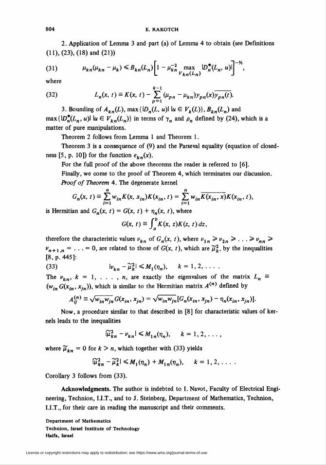
2. Application of Lemma 3 and part (a) of Lemma 4 to obtain (see Definitions

(11), (23), (18) and (21))

(31) Vkn(Pkn-Vk)<Bkn(.Ln)\1-tâ maX LD*(¿„, m)M ,L vkn(Ln) J

wherefc-i _

(32) Ln(x, t) = K(X, t)~Z (Vpn - Vkn)ypn(x)ypn(t)-P-l

3. Bounding of Akn(L), max{lD„(L, m)I Im G Vk(L)},Bkn(L„) and

max{\D*(Ln, u)\ Im G Vkn(Ln)} in terms of yn and pn defined by (24), which is a

matter of pure manipulations.

Theorem 2 follows from Lemma 1 and Theorem 1.

Theorem 3 is a consequence of (9) and the Parseval equality (equation of closed-

ness [5, p. 10]) for the function ek„(x).

For the full proof of the above theorems the reader is referred to [6].

Finally, we come to the proof of Theorem 4, which terminates our discussion.

Proof of Theorem 4. The degenerate kernel

n n _

G„(X, t) = Z WinK(x, Xin)K(xin, t)=Z winK(Xin' x)K(xin> 0.i-l 1=1

is Hermitian and Gn(x, t) = G(x, t) 4 nn(x, t), where

G(x, t) = ("k(x, z)K(z, t)dz,J a

therefore the characteristic values vkn of Gn(x, t), where vln > v2n > . . . > vnn >

vn + i,n = ■ ■ ■ = 0. are related to those of G(x, t), which are /I2, by the inequalities

[8, p.'445]:

(33) \vkn -jSgKüf!(*„), k=l,2,....

The vkn, k = 1, . . . , 7i, are exactly the eigenvalues of the matrix Ln =

(win G(xin, xn)), which is similar to the Hermitian matrix A^"' defined by

Af =^WinWjnG(Xin>Xjn) = ^winWjnlG„(xin, Xjn) - T}n(x¡n, Xjn)].

Now, a procedure similar to that described in [8] for characteristic values of ker-

nels leads to the inequalities

$kn -"kJ^MmÜn), k=l,2,...,

where pkn = 0 for k > n, which together with (33) yields

ÍT2„-M2KM1(7,„)+M1„(t?„), *-l,2.

Corollary 3 follows from (33).

Acknowledgments. The author is indebted to I. Navot, Faculty of Electrical Engi-

neering, Technion, I.I.T., and to J. Steinberg, Department of Mathematics, Technion,

I.I.T., for their care in reading the manuscript and their comments.

Department of Mathematics

Technion, Israel Institute of Technology

Haifa, Israel



1. K. E. ATKINSON, "The numerical solution of the eigenvalue problem for compact integral

operators," Trans. Amer. Math. Soc., v. 129, 1967, pp. 458-465. MR 36 #3172.

2. C. T. H. BAKER, "The deferred approach to the limit for eigenvalues of integral equa-

tions," SIAM J. Numer. Anal, v. 8, 1971, pp. 1-10. MR 48 #3276.

3. H. BRAKHAGE, "Zur Fehlerabshatzung fur die numerische Eigenwertbestimmung bei In-

tegralgleichungen," Numer. Math., v. 3, 1961, pp. 174-179. MR 23 #A2185.

4. P. LINZ, "On the numerical computation of eigenvalues and eigenvectors of symmetric in-

tegral equations," Math. Comp., v. 24, 1970, pp. 905-910. MR 43 #1461.

5. S. G. MIHLIN, Lectures on Linear Integral Equations, Fizmatgiz, Moscow, 1959; English

transi., Russian Monographs and Texts on Advanced Math, and Phys., vol. 2, Gordon and Breach,

New York; Hindustan, Delhi, 1960. MR 23 #A490; 24 #A3483.

6. E. RAKOTCH, Numerical Solution for Eigenvalues and Eigenfunctions of a Hermitian Ker-

nel and an Error Estimate, Technical Report No. 38, Department of Computer Science, Technion,

I.I.T, November 1974.

7. J. TODD, Introduction to the Constructive Theory of Functions, Academic Press, New

York, 1963. MR 27 #6061.

8. H. WEYL, "Das asymptotische Verteilungsgesetz der Eigenwerte linearer partieller Differen-

tialgleichungen (mit einer anwendung auf die Theorie der Hohlraumstrahlung)," Math. Ann., v. 71,

1912, pp. 441-479.

9. H. WIELANDT, Error Bounds for Eigenvalues of Symmetric Integral Equations, Proc.

Sympos. Appl. Math., vol. 6, Amer. Math. Soc, Providence, R. I., 1956, pp. 261-282. MR 19, 179.


Numerical Solution for Eigenvalues and Eigenfunctions of a ...the eigenvalues pkn, k = 1, . . . ,...

Documents

Transcript of Numerical Solution for Eigenvalues and Eigenfunctions of a ...the eigenvalues pkn, k = 1, . . . ,...