Numerical Simulation of Two–Dimensional Flow Past a Dimpled ...

Applied Mathematical Sciences, Vol. 5, 2011, no. 34, 1649 - 1667

Numerical Simulation of Two–Dimensional

Flow Past a Dimpled Cylinder Using

a Pseudospectral Method

M. Kotovshchikova

Department of MathematicsUniversity of Manitoba

Winnipeg, Manitoba R3T 2N2, [email protected]

S. H. Lui

Department of MathematicsUniversity of Manitoba

Winnipeg, Manitoba R3T 2N2, [email protected]

Abstract

A numerical simulation of steady and unsteady two-dimensional

flows past cylinder with dimples based on highly accurate pseudospec-

tral method is the subject of the present paper. The vorticity and

streamfunction formulation of two-dimensional incompressible Navier-

Stokes equations with no-slip boundary conditions is used. The sys-

tem is formulated on a unit disk using curvilinear body fitted coor-

dinate system. Key issues of the curvilinear coordinate transforma-

tion are discussed, to show its importance in properly defined node

distribution. For the space discretization of the governing system the

Fourier-Chebyshev pseudospectral approximation on a unit disk is im-

plemented. For steady flow simulations the non-linear time-independent

Navier-Stokes problem is solved using the Newton’s method. For the

time-dependent problem the semi-implicit third order Adams-Bashforth

backward differentiation scheme is used. Finally numerical result for

both steady and unsteady problems are presented. A comparison of re-

sults for the smooth cylinder with those from other authors shows good

agreement. Spectral accuracy is demonstrated using the steady solver.

Mathematics Subject Classification: 65M70, 35Q30, 76D17

1650 M. Kotovshchikova and S. H. Lui

Keywords: Incompressible viscous flow, Navier–Stokes equations, circularcylinder, pseudospectral method, streamfunction–vorticity, von Karman street

1 Introduction

Flow over a circular cylinder has been under intensive experimental and numer-ical investigations for many decades. Among some reasons for its popularityare the simplicity of geometry and interesting flow features: steady stable vor-tices behind the cylinder at low Reynolds number, bifurcation into a stableoscillatory wake at higher Reynolds number, bifurcation into flows with three–dimensional structures with a further increase in Reynolds number and finallydevelopment into turbulence at still higher Reynolds number.

While most of the numerical simulations employ either the finite differ-ence or finite element discretization, we use a Fourier–Chebyshev collocationmethod to obtain a spectrally accurate solution. We also map the flow do-main into the interior of the unit disk which means that there is no need toimpose any non–physical boundary condition at the artificial boundary of thefinite computational domain in most other studies. As a by product, it is notmuch more difficult to simulate domains whose outer boundary is given byr = g(θ) where (r, θ) are the polar coordinates and g is a smooth function. Forinstance, the boundary of a dimpled cylinder (two–dimensional golf ball) canbe modeled by r = 1 + ε cosnθ for some integer n.

See [30] for a review of dynamics of flow over a cylinder. Some importantmonographs on spectral methods include [1], [2], [5], [11], [14], [15], [18], [22],[28]. Works on finite difference simulations of flow over a cylinder include[4], [10], [13], [17], [24], [25]. Some representative papers on finite elementsimulations include [6], [12], [20]. Spectral collocation method has been usedby [8], [21], [27], [29], among others. [3] uses finite volumes while [31] employsa least–squares meshfree method. A lattice Boltzmann approach was taken in[16]. This list is just the tip of the iceberg of studies on this problem and manyimportant papers have been omitted.

There is also a large community interested in turbulence in this problem.See, for instance, [7], [19], [26] and the references therein.

All papers known to us carry out the computations in a truncated physicaldomain except for [17] which transforms the domain to a rectangle. Exceptfor [4], most have simulation results for flow over simple objects such as disksor ellipses. A dimpled cylinder imposes an additional challenge to an alreadycomplicated problem.

We focus on the two–dimensional problem. For Reynolds numbers smallerthan about 190, all flow features are known to be intrinsically two–dimensional.Three-dimensional effects become important at higher Reynolds numbers.

Numerical simulation of two–dimensional flow 1651

2 Problem Formulation

Assume the fluid is viscous and incompressible. The domain of interest isexterior to an object with boundary given by r = a + ε cos(kθ) where (r, θ)are the polar coordinates. Here a and ε are positive with ε � a in case of agolf ball (although this fact is not explicitly needed). Assume that the objectis stationary in a uniform external flow with constant velocity U at infinityin the direction of the positive x–axis. The two–dimensional non–dimensionalNavier–Stokes equations in the streamfunction–vorticity formulation is

∂ω

∂t=

2

Re4ω +G(ω, ψ),

0 = −4ψ − ω,

where G(ω, ψ) is the Jacobian |∂(ω,ψ)∂(x,y)

|, and the Reynolds number is

Re =ρU2a

µ

with ρ, µ representing the density and dynamic viscosity while U is the uniformvelocity of the flow at infinity. After non–dimensionalization, it is assumed thata = 1 and U = 1.

There are two boundary conditions for the streamfunction ψ:

ψ = 0 =∂ψ

∂ν

along Γ, the boundary of the object and no boundary condition for the vorticityω. At infinity,

ψ → y + C, ω → 0,

where C is a constant. In fact C = 0 since the streamline along the x–axisfrom −∞ to the stagnation point on Γ implies that ψ = C = 0.

For computations, most authors truncate the domain at some large ra-dius and apply some unphysical numerical boundary condition at the artificialinterface. It is well documented that this can pollute the solution near theboundary of the object. We map the domain exterior to the object to the in-terior of the unit disk, with infinity mapped to the origin. One small obstacleis that the value of ψ at infinity is y which cannot be mapped in a one–to–onefashion to a unique value at the centre of the disk. One simple solution is tomake a change of variable from ψ to ψ−y so that the new variable approacheszero at infinity.

Consider the simplest case ε = 0. That is the object is the unit disk. Thenaive mapping (r, θ) → (R, θ) where R = r−1 takes the domain exterior to thedisk to the interior of the disk. Now if the Fourier–Chebyshev pseudospectral


method is used to solve the problem inside the disk, then since the nodescluster near the boundary, this corresponds to an overly dense set of nodesnear the boundary and not enough nodes in the region far from the boundary( see figure 1 ).

In general, let the boundary of the object be described by

(x, y) = γ(θ) (cos θ, sin θ)

for some smooth function γ. Take the transformation from the computationaldomain to the physical domain as

(x, y) =W (R, θ) = f(R)γ(θ) (cos θ, sin θ).

The function f is twice continuously differentiable and maps the interval [0, 1]to [1,∞). It is reasonable to require that f satisfies the following constraints

f(1) = 1,

limR→0+

f(R) = ∞,

∂f

∂R< 0.

As remarked above, f(R) = R−1 is not appropriate for our purposes. One guid-ance is that the Laguerre function e−x/2Ln(x) where Ln is the n–th Laguerrepolynomial is the appropriate orthogonal function used in spectral method onthe interval [1,∞). Hence it is reasonable to take f(R) = 1 − c lnR for somepositive c. This map gives a good distribution of nodes far from the object. To

get a good spacing near the cylinder, we use the rational map b1− R

1 +Rwhere

b > 0. Thus a map which can accommodate a general distribution is thecombination

f(R) = 1− c lnR + b1 −R

1 +R. (1)

On the unit disk, the naive Fourier–Chebyshev pseudospectral method ex-pands a function as a double summation with Chebyshev polynomials in theradial variable R ∈ [0, 1] and Fourier modes in the angular variable θ ∈ [0, 2π).This is wasteful because of a clustering of nodes near the origin. Fornberg [14]proposes an elegant solution where R ∈ [−1, 1] and θ ∈ [0, π]. When R ∈ (0, 1]and θ ∈ (π, 2π), we define

u(−R, θ − π) = u(R, θ).


Figure 1: The difference in the distribution of nodes for maps f(R) = 1 −c lnR + b1−R

1+Rand f(R) = 1

Rfor the number of grid points r × θ = 41 × 40,

here c=2, b=60.

3 Numerical Results

All numerical experiments were performed in MATLAB. To determine thecoefficients b and c of the map 1 we use the distribution of Laguerre points onthe interval [1,∞) with a scaling parameter s. Let ln be the set of n Laguerrecollocation nodes. Define points by

Lnj =

{

1, j = 01 + s

nlnj, j = 1, ..., n

The values of b and c are determined by the least square approximation ofpoints f(Rnj) to Lnj . In our computations we use the value s between 20 and30.

Steady state flow simulations were obtained by solving the steady Navier-Stokes equations using Newton’s method. As a benchmark for the steady state


solutions, simulated flows were compared with experimental [9] and numerical[10, 13, 25] results reported in the literature.

For the steady fluid flow past a circular cylinder, the characteristic quan-tities usually include the drag coefficient CD, the separation angle θs and thewake length Lw. The wake length, Lw is the distance between the rear ofthe cylinder to the end of the separated region. It can be measured usingthe x-component of the velocity u along the x-axis, which changes its sign atthe point where wake ends. The separation angle θs can be determined fromzero-vorticity at the surface of the cylinder. The drag coefficient on a circularcylinder can be computed by

CD = −1

2

∫ 2π

0

(p)R=1 cos θdθ −2

Re

∫ 2π

0

(ω)R=1 sin θdθ, (2)

where p and ω are dimensionless pressure and vorticity on the cylinder surface.The computations were done for 10 ≤ Re ≤ 40 on grids with size 61× 60 andclustering parameter s = 20, 30, and results for the wake length, separationangle , drag and vorticity on the boundary are shown in figures 2, 3, 4 and5 respectively. Results demonstrate good agreement with reference numerical[10, 13, 25] and experimental [9] data reported by other authors.

Figure 2: Wake length Lw over the diameter d = 2 for the steady flow pastcircular cylinder compared with results of Dennis & Chang [10], Takami &Keller [25] and Coutanceau & Bouard [9].


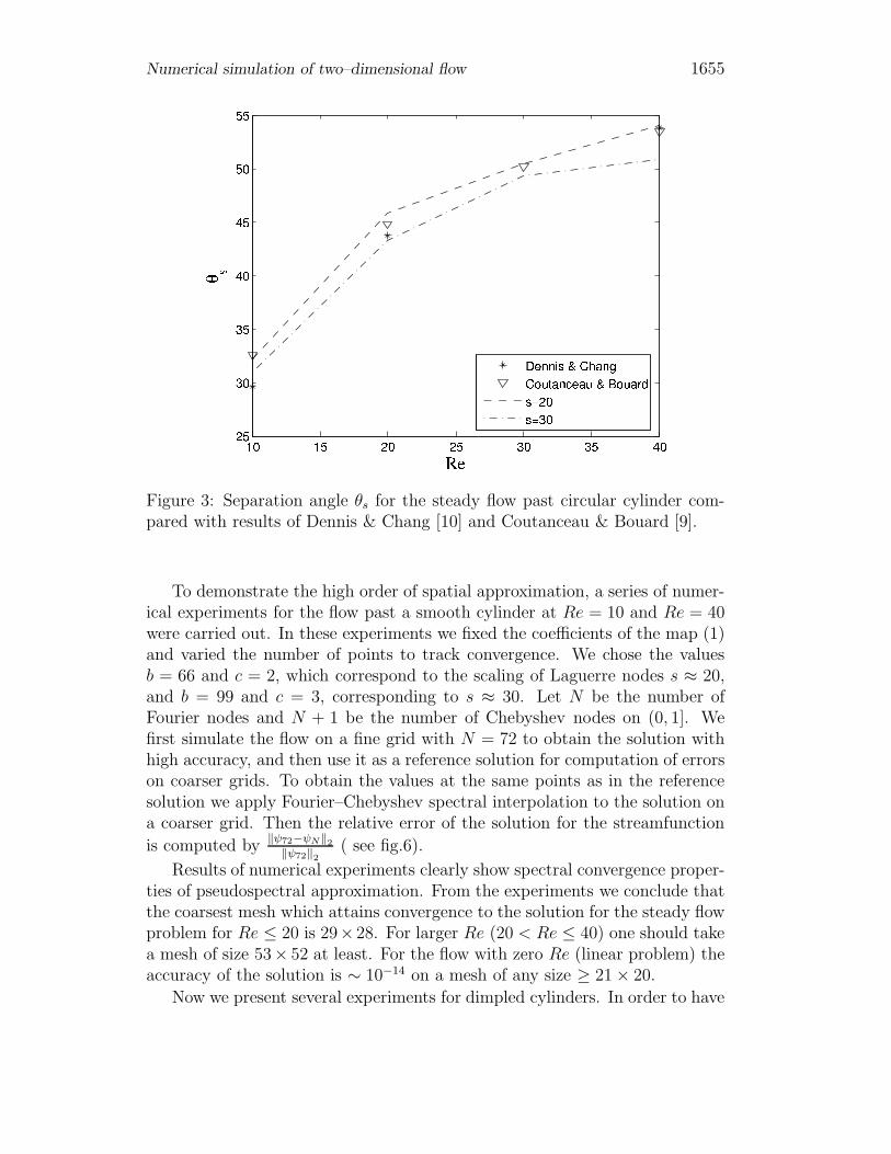
Figure 3: Separation angle θs for the steady flow past circular cylinder com-pared with results of Dennis & Chang [10] and Coutanceau & Bouard [9].

To demonstrate the high order of spatial approximation, a series of numer-ical experiments for the flow past a smooth cylinder at Re = 10 and Re = 40were carried out. In these experiments we fixed the coefficients of the map (1)and varied the number of points to track convergence. We chose the valuesb = 66 and c = 2, which correspond to the scaling of Laguerre nodes s ≈ 20,and b = 99 and c = 3, corresponding to s ≈ 30. Let N be the number ofFourier nodes and N + 1 be the number of Chebyshev nodes on (0, 1]. Wefirst simulate the flow on a fine grid with N = 72 to obtain the solution withhigh accuracy, and then use it as a reference solution for computation of errorson coarser grids. To obtain the values at the same points as in the referencesolution we apply Fourier–Chebyshev spectral interpolation to the solution ona coarser grid. Then the relative error of the solution for the streamfunction

is computed by‖ψ72−ψN‖

2

‖ψ72‖2( see fig.6).

Results of numerical experiments clearly show spectral convergence proper-ties of pseudospectral approximation. From the experiments we conclude thatthe coarsest mesh which attains convergence to the solution for the steady flowproblem for Re ≤ 20 is 29×28. For larger Re (20 < Re ≤ 40) one should takea mesh of size 53× 52 at least. For the flow with zero Re (linear problem) theaccuracy of the solution is ∼ 10−14 on a mesh of any size ≥ 21× 20.

Now we present several experiments for dimpled cylinders. In order to have


Figure 4: Drag coefficient CD for the steady flow past circular cylinder com-pared with Dennis & Chang [10] and Takami & Keller [25].

enough memory space to store dense matrices, experiments were carried outfor 4 and 8 dimples. For the larger number of dimples the grid size has to belarge enough to handle small–scale vortices. It was observed, that the numberof grid points per dimple in angular direction M has to be 4-6 in order toobtain reasonable results with good resolution of the flow. In our simulationsthe grid size was 61× 48.

To study the influence of dimples on a steady state flow characteristics weperformed a series of computations: for k = 4 and for k = 8, with ε = π/(8k)in both cases. For 10 ≤ Re ≤ 40 we recorded the drag coefficient CD, theseparation angle θs and the wake length Lw. See fig. 7, 8 and 9.

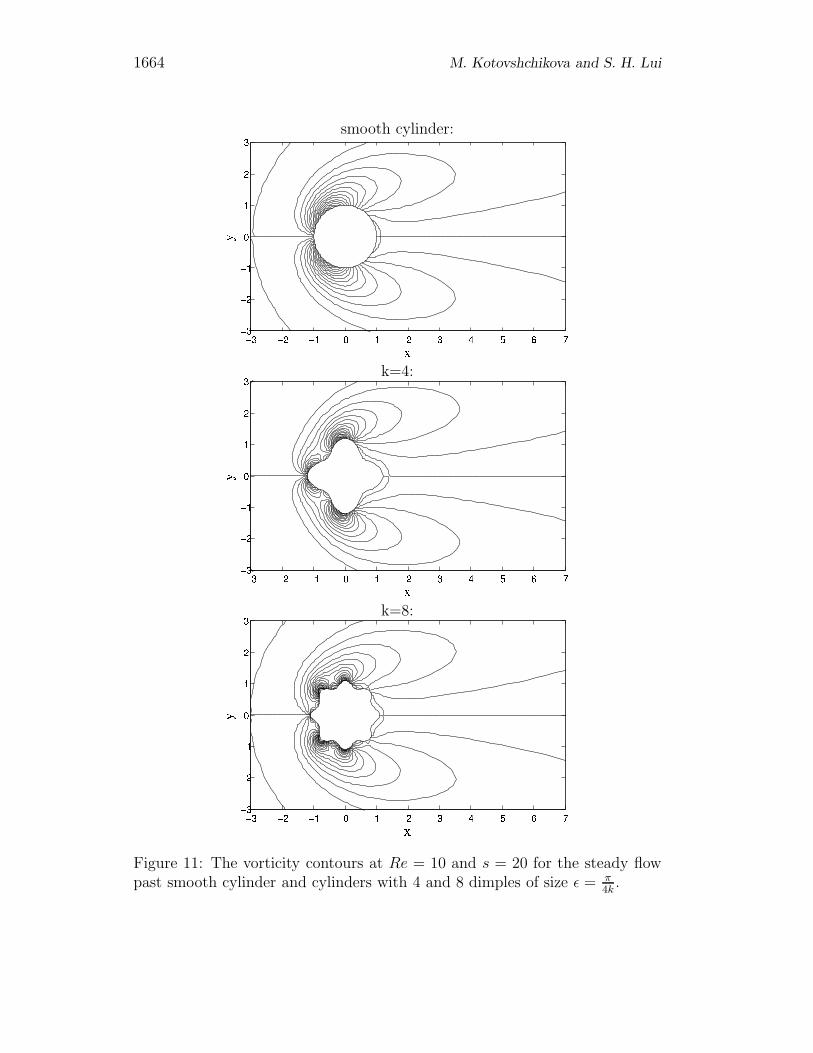
Below we present flow pictures at Re = 10 for a smooth cylinder andcylinders with 4 and 8 dimples of size ε = π/(4k), which means the depth ofeach dimple (= 2ε) is 4 times smaller then its width (= 2π/k). See fig.10 andfig.11.

For the unsteady flow simulations the 3–rd order semi–implicit scheme isused, in which Adams-Bashforth extrapolation is applied to the non–linear partof the vorticity equation and the time derivative is approximated by backwarddifferentiation:(

11

6∆t+

2

Re∆

)

ωl+1 = 3G(φl, ωl)− 3G(φl−1, ωl−1) +G(φl−2, ωl−2) +3

∆tωl−


Figure 5: Vorticity on the boundary ωb for the steady flow past circular cylindercompared with results of Dennis & Chang [10] and Fornberg [13].

−3

2∆tωl−1 +

1

3∆tωl−2.

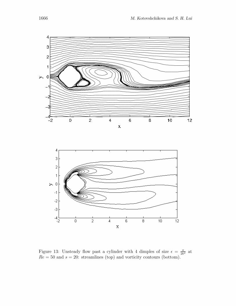
Some qualitative results for unsteady flows past smooth and dimpled cylin-ders are shown below on fig.12, 13 and fig.14 by plots of streamfunction andvorticity. The mesh size in case of smooth cylinder is 41× 60 and for the dim-pled cylinders it is 41×40. The time step varies between 0.02 and 0.025. As weincrease Re or grid–size we have to take smaller time–steps and computationsbecome costly in terms of time.

4 Conclusion

Our strategy of mapping the exterior physical domain to the interior of theunit disk is a good one in theory since it relieves us of determining the locationof the far–field boundary as well as the boundary condition there. In practice,we found that our method is somewhat sensitive to the choice of parameter inour mapping. Since there does not appear to be any guideline to choose theseparameters, our conclusion is that the present method is not superior to themethod of truncation of the domain.

The present method can be improved in many ways. First, all the impor-tant physics are downstream and so instead of having a uniform grid in the


Figure 6: Spectral convergence of the solution for the flow at Re=10, 40.

angular direction, it is more efficient to have more nodes behind the body. [2]proposes a map

ξ(θ) = 2 arctan

(

K tanθ

2

)

, θ ∈ [−π, π]

where K is a stretching parameter. This allows for a clustering of nodes nearthe angle 0.

To simulate flow at higher Reynolds, a domain decomposition techniquewill be necessary. The region close to the body is still modeled by the viscousNavier–Stokes while elsewhere, the Euler equations can be used. The exchangeof data between the two regions is a non–trivial issue. See [23]. Of course, atthese higher Reynolds numbers, the three–dimensional model must be solved.

ACKNOWLEDGEMENTS. This work was in part supported by grantsfrom NSERC of Canada and URGP of University of Manitoba.

References

[1] C. Bernardi and Y. Maday. Spectral methods. In P. G. Ciarlet and J. L.Lions, editors, Handbook of Numerical Analysis, volume 5, Amsterdam,1997. North-Holland.


Figure 7: Drag coefficient for the steady flow past smooth and dimpled cylin-ders.

[2] J. P. Boyd. Chebyshev and Fourier Spectral Methods, 2nd rev. ed. Dover,Mineola, New York, 2001.

[3] M. Braza, P. Chassaing, and H. H. Minh. Numerical study and physicalanalysis of the pressure and velocity fields in the near wake of a circularcylinder. J. Fluid Mech., 284:79–130, 1995.

[4] D. Calhoun. A Cartesian grid method for solving the two–dimensionalstreamfunction–vorticity equations in irregular regions. J. Comput. Phys.,176:231–275, 2002.

[5] C. Canuto, M. Y. Hussaini, A. Quarteroni, and T. A. Zang. SpectralMethods in Fluid Dynamics. Springer-Verlag, New York, 1988.

[6] J.H. Chen, W.G. Pritchard, and S.J. Tavener. Bifurcation for flow past acylinder between parallel planes. J. Fluid Mech., 284:23–41, 1995.

[7] G. Constantinescu and K. Squires. Numerical investigations of flow over asphere in the subcritical and supercritical regimes. Phys. Fluids, 16:1449–1466, 2004.

[8] R. Corral and J. Jimenez. Fourier/Chebyshev methods for the incom-pressible Navier–Stokes equations in infinite domains. J. Comput. Phys.,121:261–270, 1995.


Figure 8: Separation angle for the steady flow past smooth and dimpled cylin-ders.

[9] M. Coutanceau and R. Bouard. Experimental determination of the mainfeatures of the viscous flow in the wake of a circular cylinder in uniformtranslation: steady flow. J. Fluid Mech., 79:231–256, 1977.

[10] S.C.R. Dennis and G. Z. Chang. Numerical solutions for steady flowpast a circular cylinder at Reynolds numbers up to 100. J. Fluid Mech.,42:471–490, 1970.

[11] M. O. Deville, P. F. Fischer, and E. H. Mund. High–Order Methods forIncompressible Fluid Flow. Cambridge University Press, Cambridge, 2002.

[12] Y. Ding and M. Kawahara. Three–dimensional linear stability analysisof incompressible viscous flows using the finite element method. Int. J.Numer. Meth. Fluids, 31:451–479, 1999.

[13] B. Fornberg. A numerical study of steady viscous flow past a circularcylinder. J. Fluid Mech., 98:819–855, 1980.

[14] B. Fornberg. A Practical Guide to Pseudospectral Methods. CambridgeUniversity Press, Cambridge, 1996.

[15] D. Funaro. Spectral Elements for Transport-Dominated Equations.Springer-Verlag, Berlin Heidelberg, 1997.


Figure 9: Wake length for the steady flow past smooth and dimpled cylinders.

[16] X. He and G. Doolen. Lattice boltzmann method on curvilinear coordi-nates system: Flow around a circular cylinder. J. Comput. Phys., 134:306–315, 1997.

[17] D.B. Ingham and T. Tang. A numerical investigation into the steadyflow past a rotating circular cylinder at low and intermediate Reynoldsnumbers. J. Comput. Phys., 87:91–107, 1990.

[18] G. Karniadakis and S. Sherwin. Spectral/hp Element Methods for Compu-tational Fluid Dynamics, 2nd ed. Oxford University Press, Oxford, 2005.

[19] A. G. Kravchenko and P. Moin. Numerical studies of flow over a circularcylinder at red = 3900. Phys. Fluids, 12:403–417, 2000.

[20] B. Kumar and S. Mittal. Effect of blockage on critical parameters for flowpast a circular cylinder. Int. J. Numer. Meth. Fluids, 50:987–1001, 2006.

[21] R. Mittal. A Fourier–Chebyshev spectral collocation method for sim-ulating flow past spheres and spheroids. Int. J. Numer. Meth. Fluids,30:921–937, 1999.

[22] R. Peyret. Spectral Methods for Incompressible Viscous Flow. Springer-Verlag, New York, 2002.


[23] A. Quarteroni and A. Valli. Domain Decomposition Methods for PartialDifferential Equations. Oxford University Press, Oxford, 1999.

[24] E. Stalberg, A. Bruger, P. Lotstedt, A. V. Johansson, and D. S. Henning-son. High order accurate solution of flow past a circular cylinder. J. Sci.Comput., 27:431–441, 2006.

[25] H. Takami and H. B. Keller. Steady two–dimensional viscous flow of anincompressible fluid past a circular cylinder. Phys. Fluids Suppl., 12:11–51, 1969.

[26] A.G. Tomboulides and S. A. Orszag. Numerical investigation of transi-tional and weak turbulent flow past a sphere. J. Fluid Mech., 416:45–73,2000.

[27] D.J. Torres and E.A. Coutsias. Pseudospectral solution of the two–dimensional Navier–Stokes equations in a disk. SIAM J. Sci. Comput.,21:378–403, 1999.

[28] L. N. Trefethen. Spectral Methods in Matlab. SIAM, Philadelphia, 2000.

[29] T. Warburton, L. F. Pavarino, and J. S. Hesthaven. A pseudo-spectralscheme for the incompressible navier–stokes equations using unstructurednodal elements. J. Comput. Phys., 164:1–21, 2000.

[30] C.H.K. Williamson. Vortex dynamics in the cylinder wake. Annu. Rev.Fluid Mech., 28:477–539, 1996.

[31] X.K. Zhang, K.C. Kwon, and S.K. Youn. The least–squares meshfreemethod for the steady incompressible viscous flow. J. Comput. Phys.,206:182–207, 2005.

Received: September, 2010


smooth cylinder:

k=4:

k=8:

Figure 10: Streamlines at Re = 10 and s = 20 for the steady flow past smoothcylinder and cylinders with 4 and 8 dimples with size ε = π

4k.


smooth cylinder:

k=4:

k=8:

Figure 11: The vorticity contours at Re = 10 and s = 20 for the steady flowpast smooth cylinder and cylinders with 4 and 8 dimples of size ε = π

4k.


Figure 12: Unsteady flow past a smooth cylinder at Re = 100 and s = 25:streamlines (top) and vorticity contours (bottom).


Figure 13: Unsteady flow past a cylinder with 4 dimples of size ε = π2k2

atRe = 50 and s = 20: streamlines (top) and vorticity contours (bottom).


Figure 14: Unsteady flow past a cylinder with 10 dimples of size ε = πk2

atRe = 50 and s = 20: streamlines (top) and vorticity contours (bottom).

Numerical Simulation of Two–Dimensional Flow Past a Dimpled ...

Documents

Transcript of Numerical Simulation of Two–Dimensional Flow Past a Dimpled ...