Numerical Simulation of TurbulentAccelerated Round Jets for Aeronautical

Applications

Pedro Miguel Rosa Ferreira Neto

Masters thesis on

Aerospace Engineering

Jury

President: Prof. Fernando Jose Parracho Lau

Supervisor: Prof. Jose Carlos Fernandes Pereira

Supervisor: Dr. Carlos Bettencourt da Silva

Examiner: Prof. Joao Manuel Goncalves de Sousa Oliveira

November of 2008

Acknowledgments

I would like to express my gratitude to my supervisors, Carlos Bettencourt da Silva,

for his orientation and knowledge sharing on what was my entrance to the world of

turbulence, and Jose Carlos Pereira, for his expertise and for the magnificent way he

teaches fluid mechanics and computational fluid dynamics.

Thank you to everyone at LASEF, for all the tips and tricks, and for the very good

working experience.

A very special thanks to Joana, for her invaluable help and support throughout my

thesis and all the years of graduation.

i

Abstract

Direct and large-eddy simulations (DNS/LES) of accelerating turbulent round jets are

used to analyze the effects of acceleration over three main subjects: the kinematics

of the coherent structures, their topology and entrainment of the jet in the near field

(x/D < 12).

The acceleration is obtained by increasing the nozzle jet velocity with time in a

previously established steady jet. Several acceleration rates and Reynolds numbers

(ReD = 500 => 1000, 1000 => 2000, and 10000 => 20000) were simulated.

Unsteady effects during acceleration include an higher shedding frequency of the pri-

mary vortex rings which also become smaller during acceleration.

Detailed acceleration maps are used to track down the kinematics of the vortex motion

in the near field of the jet. The shedding frequency increases linearly with the acceler-

ation rate which causes a number of new primary and secondary vortex merging events

in the near field of the jet that are absent from steady jets. The Reynolds number has

no influence in these unsteady effects.

The smaller primary vortex rings shed during acceleration are more stable, i.e. present

less azimuthal and radial distortion as they travel streamwise.

The acceleration decreases the spreading rate of the jet, in agreement with previous

experimental works, but contrary to previous beliefs, the entrainment rate, evaluated

in the shear layer interface, is higher during the acceleration phase of the high Reynolds

number LES simulation.

Keywords: Unsteady; Round jet; Turbulence; Coherent structures; Entrainment

ii

Resumo

Simulacoes numericas directas (DNS) e simulacoes das grandes escalas (LES) e jac-

tos acelerados turbulentos sao utilizadas para estudar os efeitos da aceleracao em tres

assuntos distintos: a cinematica das estruturas coerentes, a sua topologia e o arrasta-

mento do jacto na zona proxima (x/D < 12).

A aceleracao e obtida aumentando a velocidade de saıda do jacto ao longo do tempo, a

partir de um jacto em regime estacionario previamente estabelecido. Foram simuladas

varias taxas de aceleracao e varios numeros de Reynolds (ReD = 500 => 1000, 1000

=> 2000, e 10000 => 20000).

Os principais efeitos da nao-estacionaridade sao um aumento da frequencia de liber-

tacao dos vortices toroidais que tambem sao menores durante a aceleracao.

Para estudar a cinematica dos turbilhoes foram criados mapas de aceleracao. Estes

permitem calcular a frequencia de libertacao e fusoes entre estruturas coerentes. A

aceleracao origina fusoes primarias e secundarias entre os vortices em anel que nao

acontecem durante as fases estacionarias das simulacoes. O numero de Reynolds nao

tem influencia nestes acontecimentos.

As estruturas coerentes libertadas durante a fase de aceleracao sao mais estaveis, isto

e, apresentam menos distorcoes radiais e azimutais enquanto viajam para jusante.

De acordo com os resultados experimentais existentes, a aceleracao diminui a taxa de

alargamento do jacto, no entanto, contrariamente a estes, o arrastamento do jacto,

medido na interface da camada de corte, aumenta durante a fase de aceleracao na

simulacao de LES a numero de Reynolds elevado.

Palavras-chave: Nao-estacionaridade; Jacto axissimetrico; Turbulencia; Estruturas

coerentes; Arrastamento

iii

Sure as I am breathing,

sure as I’m sad.

I’ll keep this wisdom in my flesh.

I leave here believing more than I had.

And there’s a reason I’ll be,

a reason I’ll be back.

Eddie Vedder

iv

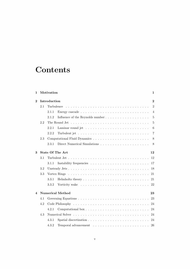
Contents

1 Motivation 1

2 Introduction 2

2.1 Turbulence . . . . . . . . . . . . . . . . . . . . . . . . . . . . . . . . . . 2

2.1.1 Energy cascade . . . . . . . . . . . . . . . . . . . . . . . . . . . . 4

2.1.2 Influence of the Reynolds number . . . . . . . . . . . . . . . . . . 5

2.2 The Round Jet . . . . . . . . . . . . . . . . . . . . . . . . . . . . . . . . 5

2.2.1 Laminar round jet . . . . . . . . . . . . . . . . . . . . . . . . . . 6

2.2.2 Turbulent jet . . . . . . . . . . . . . . . . . . . . . . . . . . . . . 7

2.3 Computational Fluid Dynamics . . . . . . . . . . . . . . . . . . . . . . . 8

2.3.1 Direct Numerical Simulations . . . . . . . . . . . . . . . . . . . . 8

3 State Of The Art 12

3.1 Turbulent Jet . . . . . . . . . . . . . . . . . . . . . . . . . . . . . . . . . 12

3.1.1 Instability frequencies . . . . . . . . . . . . . . . . . . . . . . . . 17

3.2 Unsteady Jets . . . . . . . . . . . . . . . . . . . . . . . . . . . . . . . . . 18

3.3 Vortex Rings . . . . . . . . . . . . . . . . . . . . . . . . . . . . . . . . . 21

3.3.1 Helmholtz theory . . . . . . . . . . . . . . . . . . . . . . . . . . . 21

3.3.2 Vorticity wake . . . . . . . . . . . . . . . . . . . . . . . . . . . . 22

4 Numerical Method 23

4.1 Governing Equations . . . . . . . . . . . . . . . . . . . . . . . . . . . . . 23

4.2 Code Philosophy . . . . . . . . . . . . . . . . . . . . . . . . . . . . . . . 24

4.2.1 Computational box . . . . . . . . . . . . . . . . . . . . . . . . . . 24

4.3 Numerical Solver . . . . . . . . . . . . . . . . . . . . . . . . . . . . . . . 24

4.3.1 Spatial discretization . . . . . . . . . . . . . . . . . . . . . . . . . 24

4.3.2 Temporal advancement . . . . . . . . . . . . . . . . . . . . . . . 26

v

4.3.3 Pressure-velocity coupling . . . . . . . . . . . . . . . . . . . . . . 26

4.3.4 LES sub-grid scale model . . . . . . . . . . . . . . . . . . . . . . 27

4.4 Boundary Conditions . . . . . . . . . . . . . . . . . . . . . . . . . . . . . 28

4.4.1 Lateral boundaries . . . . . . . . . . . . . . . . . . . . . . . . . . 28

4.4.2 Inlet condition . . . . . . . . . . . . . . . . . . . . . . . . . . . . 28

4.4.3 Outlet condition . . . . . . . . . . . . . . . . . . . . . . . . . . . 30

5 Linear Acceleration of Turbulent Round Jets 32

5.1 Simulations . . . . . . . . . . . . . . . . . . . . . . . . . . . . . . . . . . 32

5.2 Overview of the Base Simulation . . . . . . . . . . . . . . . . . . . . . . 34

5.3 Kinematics of the Vortex Motion . . . . . . . . . . . . . . . . . . . . . . 39

5.3.1 Acceleration maps . . . . . . . . . . . . . . . . . . . . . . . . . . 39

5.3.2 Influence of the Reynolds number . . . . . . . . . . . . . . . . . . 40

5.3.3 Vortex ring merging events . . . . . . . . . . . . . . . . . . . . . 41

5.3.4 Characteristic frequencies . . . . . . . . . . . . . . . . . . . . . . 44

5.4 Topology of the Vortex Rings . . . . . . . . . . . . . . . . . . . . . . . . 47

5.4.1 Influence of the acceleration rate . . . . . . . . . . . . . . . . . . 51

5.5 Jet Entrainment . . . . . . . . . . . . . . . . . . . . . . . . . . . . . . . 52

5.5.1 Jet width - δ0.5 . . . . . . . . . . . . . . . . . . . . . . . . . . . . 52

5.5.2 Streamwise mass flow rate . . . . . . . . . . . . . . . . . . . . . . 53

5.5.3 Radial velocity - Shear layer interface . . . . . . . . . . . . . . . 54

5.6 Deccelerated Jets . . . . . . . . . . . . . . . . . . . . . . . . . . . . . . . 58

6 Conclusion 59

6.1 Kinematics of Vortex Motion and Topology of the Vortex Rings . . . . . 59

6.1.1 Shear layer mode . . . . . . . . . . . . . . . . . . . . . . . . . . . 59

6.1.2 Preferred mode . . . . . . . . . . . . . . . . . . . . . . . . . . . . 61

6.1.3 Secondary instabilities . . . . . . . . . . . . . . . . . . . . . . . . 62

6.2 Entrainment Rate . . . . . . . . . . . . . . . . . . . . . . . . . . . . . . 62

A Q Criteria Visualization 64

B Article no. 1 72

Bibliography 77

vi

List of Figures

2.1 Flow past a cylinder at different Reynolds numbers, from Frisch [19] . . 3

2.2 Energy spectra, from Geurts [20] . . . . . . . . . . . . . . . . . . . . . . 4

2.3 Sketch of a round jet . . . . . . . . . . . . . . . . . . . . . . . . . . . . . 6

2.4 Round jet at different Reynolds numbers, from Kwon & Seo [28] . . . . 8

2.5 Cost of computing since 1945, from Moravec [38] . . . . . . . . . . . . . 9

2.6 Filtering f(x), from Frisch [19] . . . . . . . . . . . . . . . . . . . . . . . 11

3.1 Spreading rate results from Kwon & Seo [28] and Bogey & Baily [2] . . 13

3.2 The Kelvin-Helmholtz instability, from Brederode [14] . . . . . . . . . . 14

3.3 Spatial growth rate −αi as a function of the frequency β: axissymmet-

ric mode (continuous) and helical (dashed) modes, from Michalke &

Hermann [36] . . . . . . . . . . . . . . . . . . . . . . . . . . . . . . . . . 15

3.4 Both preferred mode shapes in a round jet DNS from the present study 15

3.5 Azimuthal instability in a vortex ring, from Van Dyke [17] . . . . . . . . 16

3.6 Draft illustrating lateral jets formation, from Bancher et al [3] . . . . . 17

3.7 Normalized entrainment from Roy & Johari computational results [42] . 20

3.8 Concentration front on experiment by Zhang & Johari [50] . . . . . . . . 21

3.9 Aproximate sketch of the vortex rings in a round jet, from Abani &

Reitz [1] . . . . . . . . . . . . . . . . . . . . . . . . . . . . . . . . . . . . 21

3.10 Instantaneous streamlines and vorticity patches (vortex ring frame of

reference), from Dabiri & Gharib [12] . . . . . . . . . . . . . . . . . . . . 22

4.1 Sketch of the Uforc component in the inlet profile, from Urbin & Metais

[45] . . . . . . . . . . . . . . . . . . . . . . . . . . . . . . . . . . . . . . . 30

5.1 Inlet Reynolds number ReD evolution for some simulations . . . . . . . 33

5.2 Centerline slice with contour of Q > 0.01 prior to the acceleration . . . . 35

5.3 Iso-surfaces of positive Q . . . . . . . . . . . . . . . . . . . . . . . . . . . 36

vii

5.4 Centerline slice with contour of Q > 0.01 during the acceleration . . . . 36

5.5 Centerline slice with contour of Q > 0.01 at the end of acceleration . . . 37

5.6 Centerline slice with contour of Q > 0.01 after the acceleration . . . . . 37

5.7 Spectra of v during acceleration with and without the Uforc component. 38

5.8 Acceleration map of the base simulation, α = 0.06, ReiD = 500 . . . . . 39

5.9 Acceleration maps . . . . . . . . . . . . . . . . . . . . . . . . . . . . . . 40

5.10 Acceleration map for α = 0.06, ReiD = 1000 . . . . . . . . . . . . . . . . 41

5.11 Acceleration map of the base simulation, α = 0.06, ReiD = 500 . . . . . 42

5.12 Height of zone A for each simulation . . . . . . . . . . . . . . . . . . . . 43

5.13 Number of primary (A) and secondary (B) merging events . . . . . . . . 43

5.14 Influence of the Reynolds number in the vortex shedding frequency for

α = 0.06 . . . . . . . . . . . . . . . . . . . . . . . . . . . . . . . . . . . . 44

5.15 Influence of the acceleration rate in the shear layer mode frequency . . . 45

5.16 Evolution of the mean shear layer mode frequency with the acceleration

rate . . . . . . . . . . . . . . . . . . . . . . . . . . . . . . . . . . . . . . 45

5.17 Structure of the jet at the last acceleration instant of the base simulation 47

5.18 Structure of the jet at the final steady stage . . . . . . . . . . . . . . . . 48

5.19 3D iso-surfaces of Q . . . . . . . . . . . . . . . . . . . . . . . . . . . . . 49

5.20 Temporal evolution of the streamwise profile of Er . . . . . . . . . . . . 50

5.21 Temporal evolution of the streamwise profile of Eθ . . . . . . . . . . . . 50

5.22 Evolution of the δ0.5 profile for α = 0.02 . . . . . . . . . . . . . . . . . . 52

5.23 δ0.5 at a given time for several α’s . . . . . . . . . . . . . . . . . . . . . 53

5.24 Streamwise evolution of Q∗ at different stages of the base simulation . . 54

5.25 Radial velocity profiles at different stages of the base simulation . . . . . 55

5.26 Entrainment profile of the ReiD = 500 simulation . . . . . . . . . . . . . 56

5.27 Entrainment profile of the ReiD = 1000 simulation . . . . . . . . . . . . 57

5.28 Entrainment profile of the ReiD = 10000 simulation . . . . . . . . . . . . 57

5.29 Acceleration map of the deceleration simulation . . . . . . . . . . . . . . 58

6.1 Sketch of the flow during the a) stationary phase, and b) accelerating

phase . . . . . . . . . . . . . . . . . . . . . . . . . . . . . . . . . . . . . 60

6.2 Dye concentration on experiment by Zhang & Johari [50] . . . . . . . . 63

viii

List of Tables

5.1 Simulations of accelerated jets performed throughout this work . . . . . 34

A.1 3D iso-surfaces of Q . . . . . . . . . . . . . . . . . . . . . . . . . . . . . 65

A.2 2D contours of positive Q during the initial phase . . . . . . . . . . . . . 66

A.3 2D contours of positive Q during acceleration . . . . . . . . . . . . . . . 67

A.4 2D contours of positive Q during the final phase . . . . . . . . . . . . . 68

A.5 Acceleration maps . . . . . . . . . . . . . . . . . . . . . . . . . . . . . . 69

A.6 Acceleration maps . . . . . . . . . . . . . . . . . . . . . . . . . . . . . . 70

A.7 Acceleration maps . . . . . . . . . . . . . . . . . . . . . . . . . . . . . . 71

ix

Chapter 1

Motivation

All turbulent flows are naturally and intrinsically unsteady, with rapid velocity fluc-

tuations, but although some of them are statistically steady, there is a class of tur-

bulent flows, in which their driving conditions are unsteady, periodic (pulsed flows),

or aperiodic (accelerated or decelerated flows), that have received much less attention

compared to the steady ones. Being inherently unsteady, these flows pose an added

difficulty in their analysis and simulation which has to be surpassed.

Examples of these flows are present both in nature and in engineering applications, such

as the blood flow, bird and insect flight, aircraft turbines, cylinder flow in alternating

engines or even as a mixture of both realms, gust flows over aircraft, for example.

The subject of this thesis is also an example of an unsteady flow, an accelerated

turbulent round jet and despite the extensive work and available studies on the steady

round jet, there are only a few works regarding the unsteady round jet.

Some examples of accelerated jet applications are VTOL (Vertical Take-Off and Land-

ing) jet aircraft, gaseous fuel injection, or any other application where jet control is

important. Still, there is no good reason not to believe that new applications, or at

least ideas, will arise once the physics of the unsteady jet are better understood.

As an effort towards that goal this work will result in two published articles, from

which the first was already submitted and is included as an appendix.

This work presents the first Direct Numerical Simulations and Large Eddy Simulations

performed of turbulent accelerated round jets.

1

Chapter 2

Introduction

Turbulent flows are the most frequently found flows on an everyday basis and round

jets are no exception to this. This chapter starts with an introduction on turbulence

and how it arises in fluid flows, followed by more specific knowledge about round jets

and turbulent round jets in particular.

2.1 Turbulence

Based on his fluid flow experiments, Osborne Reynolds (1842 - 1912) postulated the

principle of similarity for incompressible fluid flows. It states that for a given geomet-

rical shape of the boundaries, the Reynolds number is the only control parameter of

the flow. It is an adimentional number defined as:

Re =LV

ν(2.1)

Where L and V are a characteristic length and velocity, respectively, and ν is the

kinematic viscosity.

As the Reynolds number increases, so does the complexity of the flow. It loses sym-

metry and becomes more chaotic.

Take, for example, the uniform flow past a cylinder of diameter L at Re = 0.16,

Re = 26, Re = 140 and Re = 240. In the first picture, the flow at an extremely low

Reynolds number presents very smooth streamlines and almost perfect symmetry. As

2

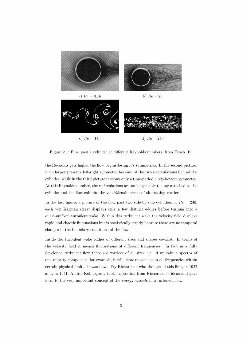
a) Re = 0.16 b) Re = 26

c) Re = 140 d) Re = 240

Figure 2.1: Flow past a cylinder at different Reynolds numbers, from Frisch [19]

the Reynolds gets higher the flow begins losing it’s symmetries. In the second picture,

it no longer presents left-right symmetry because of the two recirculations behind the

cylinder, while in the third picture it shows only a time-periodic top-bottom symmetry.

At this Reynolds number, the recirculations are no longer able to stay attached to the

cylinder and the flow exhibits the von Karman street of alternating vortices.

In the last figure, a picture of the flow past two side-by-side cylinders at Re = 240,

each von Karman street displays only a few distinct eddies before turning into a

quasi-uniform turbulent wake. Within this turbulent wake the velocity field displays

rapid and chaotic fluctuations but is statistically steady because there are no temporal

changes in the boundary conditions of the flow.

Inside the turbulent wake eddies of different sizes and shapes co-exist. In terms of

the velocity field it means fluctuations of different frequencies. In fact in a fully

developed turbulent flow there are vortices of all sizes, i.e. if we take a spectra of

one velocity component, for example, it will show movement in all frequencies within

certain physical limits. It was Lewis Fry Richardson who thought of this first, in 1922

and, in 1941, Andrei Kolmogorov took inspiration from Richardson’s ideas and gave

form to the very important concept of the energy cascade in a turbulent flow.

3

2.1.1 Energy cascade

According to this concept, most of the kinetic energy of a turbulent flow is associated

with the larger scales of motion. These get energy from the mean field inhomogeneities

and at the same time they are also transferring it to smaller and smaller scales in an

essentially inviscid and non-linear process until it gets dissipated by molecular viscosity

at the smallest scales of the flow.

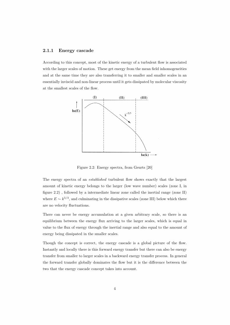
Figure 2.2: Energy spectra, from Geurts [20]

The energy spectra of an established turbulent flow shows exactly that the largest

amount of kinetic energy belongs to the larger (low wave number) scales (zone I, in

figure 2.2) , followed by a intermediate linear zone called the inertial range (zone II)

where E ∼ k5/3, and culminating in the dissipative scales (zone III) below which there

are no velocity fluctuations.

There can never be energy accumulation at a given arbitrary scale, so there is an

equilibrium between the energy flux arriving to the larger scales, which is equal in

value to the flux of energy through the inertial range and also equal to the amount of

energy being dissipated in the smaller scales.

Though the concept is correct, the energy cascade is a global picture of the flow.

Instantly and locally there is this forward energy transfer but there can also be energy

transfer from smaller to larger scales in a backward energy transfer process. In general

the forward transfer globally dominates the flow but it is the difference between the

two that the energy cascade concept takes into account.

4

2.1.2 Influence of the Reynolds number

The larger scales of motion of a given turbulent flow are usually set by any geometrical

constrains present. For example in a fluid flow inside a pipe, there cannot exist eddies

much larger than the tube’s diameter.

On the other hand, there is no geometrical constrain to the size of the smaller scales

of motion, but there is a physical one. The characteristic length of the smaller scales

is such that viscosity forces overcome inertial ones, allowing energy to be dissipated

by viscous action.

The Reynolds number, as a ratio of inertia to viscosity, therefore sets the length of the

smaller scales. At an higher Reynolds number viscosity loses importance over inertia,

so the kinetic energy must ”cascade” to smaller scales in order to allow viscosity to

become important and dissipate it.

As the larger scales do not change with the Reynolds number, it can also be understood

as a ratio of the characteristic lengths of the larger to the smaller scales of motion of

a given flow.

Kolmogorov derived an expression to the wave number of these smaller scales of motion,

which became known as the Kolmogorov dissipation scales:

η ≡(ν3

ε

)1/4

(2.2)

where ν is the kinematic viscosity and ε is the energy flux.

As previously stated the energy flux ε dissipated by the small scales is equal to the

energy flux arriving at the larger scales of the flow, it can be approximated by:

ε ∼ U3

L(2.3)

where U and L are the characteristic velocity and large scale of the flow, respectively.

2.2 The Round Jet

The round jet is one of the classic examples of a free shear layer, together with wakes

and mixing layers, and perhaps the most studied because it very frequently occurs in

nature and in industrial applications.

5

2.2.1 Laminar round jet

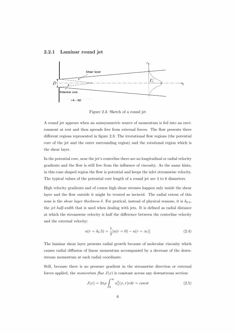
Figure 2.3: Sketch of a round jet

A round jet appears when an axissymmetric source of momentum is fed into an envi-

ronment at rest and then spreads free from external forces. The flow presents three

different regions represented in figure 2.3: The irrotational flow regions (the potential

core of the jet and the outer surrounding region) and the rotational region which is

the shear layer.

In the potential core, near the jet’s centerline there are no longitudinal or radial velocity

gradients and the flow is still free from the influence of viscosity. As the name hints,

in this cone shaped region the flow is potential and keeps the inlet streamwise velocity.

The typical values of the potential core length of a round jet are 4 to 6 diameters.

High velocity gradients and of course high shear stresses happen only inside the shear

layer and the flow outside it might be treated as inviscid. The radial extent of this

zone is the shear layer thickness δ. For pratical, instead of physical reasons, it is δ0.5,

the jet half-width that is used when dealing with jets. It is defined as radial distance

at which the streamwise velocity is half the difference between the centerline velocity

and the external velocity:

u(r = δ0.5) =12

[u(r = 0)− u(r =∞)] (2.4)

The laminar shear layer presents radial growth because of molecular viscosity which

causes radial diffusion of linear momentum accompanied by a decrease of the down-

stream momentum at each radial coordinate.

Still, because there is no pressure gradient in the streamwise direction or external

forces applied, the momentum flux J(x) is constant across any downstream section:

J(x) = 2πρ∫ ∞

0

u2x(x, r)rdr = const (2.5)

6

And as a consequence of the radial diffusion of linear momentum the mass flow rate

Q(x) grows in the streamwise direction:

Q(x) = 2πρ∫ ∞

0

ux(x, r)rdr (2.6)

∂Q(x)∂x

> 0 (2.7)

Another important quantity for the study of shear layers in general is the momentum

thickness θ(x):

θ(x) =∫ ∞

0

[u(x, r)− u∞(x)uinlet − u∞(x)

] [1− u(x, r)− u∞(x)

uinlet − u∞(x)

]dr (2.8)

where u∞ is the local streamwise velocity of the external flow and uinlet is the maximum

streamwise velocity at the jet inlet.

The jet’s momentum thickness is a measure of the momentum deficit in relation to an

ideal (inviscid) equivalent flow.

2.2.2 Turbulent jet

The majority of round jets found around us are turbulent. This happens because most

of the time there are small disturbances which get amplified causing the transition

from laminar flow to turbulent flow. These small disturbances can be ambient or inlet

noise, wall roughness in the inlet, vibrations in the mechanical structures present, or

even pressure feedback from events happening downstream in the flow.

During transition these amplified disturbances turn into primary coherent vortical

structures of toroidal shape with sizes depending on specific characteristics of the flow.

These pass through a series of division and merging events as they travel streamwise.

In a turbulent jet the radial growth of the shear layer is larger than in the laminar

jet because it is due not only to molecular viscosity but also to intermittent coherent

structures found in turbulent jets which engulf bits of irrotational fluid into the shear

layer zone. Both the effects, acting at the same time, take irrotational fluid from the

outer region into the core of the jet in a physical mechanism denominated entrainment.

Figure 2.4 presents the turbulent round jet at different Reynolds number, from a low,

almost laminar flow in picture a) to a fully turbulent jet in picture d). In the middle

pictures the jet starts as laminar and rapidly transitions to a turbulent regime:

7

a)ReD = 177 b) ReD = 437 c) ReD = 2163 d) ReD = 5142

Figure 2.4: Round jet at different Reynolds numbers, from Kwon & Seo [28]

2.3 Computational Fluid Dynamics

A long road has been covered from the second half of the twentieth century to bring

computational fluid dynamics (CFD) to the important role it plays today in the dis-

cipline of fluid dynamics as a whole. After the foundations for experimental fluid

dynamics were laid in the seventeenth century and the development of its theoretical

approach from the eighteenth century, many years had to pass before the computer

and advances in numerical methods allowed for a new revolution in the way fluid dy-

namics was studied and practiced. Today, CFD stands as an equally important tool

with theory and experiment in the solution of the problems we face today.

Advances in CFD have often been related with advances in computer technology, first

in two-dimensional methods and more recently in the three-dimensional realm. Plus,

given the rate at which computation costs are dropping since 1985, the ground is being

paved for more and more complex simulations, both in research and in the engineering

sides.

2.3.1 Direct Numerical Simulations

The available computer speed now allows for the complete Navier-Stokes equations

to be numerically calculated. This kind of simulations, where there is no modeling

whatsoever, are called Direct Numerical Simulations (DNS).

The importance of DNS comes from the way it allows to numerically study the problem

8

Figure 2.5: Cost of computing since 1945, from Moravec [38]

of turbulence, as the main idea is to use an extremely fine grid in order to calculate

all the details and structures of a turbulent flow, down to the small dissipative scales,

directly from the Navier-Stokes equations.

DNS is not suited, though, for simulation of high geometrical complexity or high

Reynolds engineering flows because current computers are not powerful enough to

perform such simulations in viable time. At the same time, from an engineering point

of view, there is rarely need for such an accuracy.

Still, DNS plays a very important role in the development of tools and simplified

models which allow the expedite simulation of complex fluid flows in an engineering

context.

Such tools, like Reynolds Averaged Navier-Stokes (RANS) simulations or, more re-

cently, Large Eddy Simulations (LES) solve a simplified form of the Navier-Stokes

equations but rely on turbulence models for accuracy. These models have been con-

siderably developed with the knowledge gained from Direct Numerical Simulations.

9

Reynolds Averaged Navier-Stokes

RANS simulations are the most usual engineering simulations nowadays. They solve

a time averaged form of the Navier-Stokes equations:

∂ui∂t

+∂uiuj∂xj

= −1ρ

∂p

∂xi+ ν

∂2ui∂x2

j

+ fi (2.9)

which, using the Reynolds decomposition, ui = ui + u′i to separate the instantaneous

quantity into its mean and fluctuating components, becomes:

∂

∂xj

(ui uj + u′iu

′j

)= −1

ρ

∂p

∂xi+ ν

∂2ui∂x2

j

+ fi (2.10)

This way the problem is simplified because what is solved is the mean velocity field,

but when the time average operation is performed on the equations the non-linear term

u′iu′j , called the turbulent stress tensor or Reynolds tensor, appears, which represents

the effect of the velocity fluctuations (i.e. turbulence) on the mean velocity field that

is being solved.

For closure, a turbulence model needs to be present. DNS plays a major role on the

development and tuning of such turbulence models.

Large-Eddy Simulations

More recently, this other type of fluid flow simulation has been gaining popularity in

the engineering scope. ”The best of both worlds” is a very good way to describe it.

Technically LES implements a way to solve only the largest scales of flow. The way

to achieve it is to apply a low-pass filter to the unsteady Navier-Stokes equations,

discarding all scales of motion below a given intermediate scale of choice which can

be big or small, depending on how much accuracy is needed. A given signal can be

separated into its large and small scale parts:

f(x) = f<K(x) + f>K(x) (2.11)

where K is the separating frequency. Figure 2.6 illustrates this procedure.

When the small scale part is discarded, one is applying a low pass filter to the signal.

The application of a spatial low pass filter to the Navier-Stokes equations results in:

∂u<i∂t

+∂u<i u

<j

∂xj= −1

ρ

∂p<

∂xi+ ν

∂2u<i∂x2

j

− ∂τij∂xi

+ f<i (2.12)

10

Figure 2.6: Filtering f(x), from Frisch [19]

In practice, this low pass filter is just a sparse mesh which is not capable of solving

all the scales of the flow, hence, one talks about grid scales (GS) which are explicitly

solved, and sub-grid scales (SGS).

The influence of the sub-grid scales on the grid-scale variables is present in the filtered

Navier-Stokes equations above through the term τij called the sub-grid scale stress

tensor:

τij = (uiuj)< − u<i u<j (2.13)

Even though LES is still computationally heavier than RANS, the fact that the larger

scale fluctuations of the velocity field are being solved (opposed to only the mean field

in RANS) allows for much more accuracy in fields where the unsteadiness of turbulence

is important, such as aeroacoustics or combustion. Regarding the latter, it is quite easy

to understand that while a RANS approach can result in a good mean concentration

field for chemical species, a LES approach might reveal a very different picture due to

unsteadiness of the results.

As in the case of turbulence models for the RANS approach, DNS plays a very impor-

tant role in the development of SGS models.

11

Chapter 3

State Of The Art

3.1 Turbulent Jet

There are several published works on the steady turbulent round jet. Some are fun-

damental studies on the physics of the jet, while others are more industry oriented

works, such as cryogenic jets or combustion hot jets, for example.

Specially important to the present work are the available steady jet’s spreading rate

results. It has been measured in several experiments and simulations over the years

and has been found to decrease as the Reynolds number increases.

For a low Reynolds number jet, it can be approximated by:

d

dx

(δ

D

)∼ x1/2 (3.1)

The most recent results are available from the experimental and numerical works of

Kwon & Seo in 2005 [28] and Bogey & Baily [2] in 2006, shown in figure 3.1.

Transition to turbulent flow

Regarding the round jet in particular, there are two instability modes with distinct

length scales Linst which govern the transition process. These are:

• Shear layer mode, Linst = θ

12

Figure 3.1: Spreading rate results from Kwon & Seo [28] and Bogey & Baily [2]

• Preferred mode, Linst = D

The shear layer instability mode happens and governs the dynamics of the jet from

the inlet to the end of the potential core where the preferred mode gains importance.

Shear layer mode

Looking very close to the jet’s inlet nozzle, moving in the radial direction, there are

the 3 different zones previously discussed, the potential core, the shear layer and the

outer irrotational zone. Due to the proximity of the inlet nozzle, the shear layer is

still very thin, much smaller than the inlet radius ( δR 1), and this makes the shear

layer quite insensitive to to curvature effects. Its initial instability characteristics are

the same of a plane mixing layer.

This initial instability is the Kelvin-Helmholtz instability, present in many other ev-

eryday examples, like in the atmosphere where clouds make it visible between layers

of air moving with different velocities, or the sea, where it is present in the interface

between the standing water and the windy air above it, not to mention recorded in

world famous pictures of Jupiter and Saturn’s colorful atmospheres.

Figure 3.2 illustrates how this instability forms in a mixing layer: If a small perturba-

tion or oscillation in the middle streamline happens to reduce the area between it and

the above streamline, the flow will accelerate in that region by continuity, decreasing

the local pressure, which pulls the central streamline further up. At the same time the

13

Figure 3.2: The Kelvin-Helmholtz instability, from Brederode [14]

flow below that streamline has decelerated, increasing the local pressure, which also

pushes the central streamline further up. Then this initial instability rolls up forming

a Kelvin-Helmohltz vortex and the process repeats itself, forming a trail of vortices

which are the primary coherent structures of turbulence and in the case of a round jet

have toroidal form.

As these vortex rings travel streamwise their core radius grows by radial viscous dif-

fusion of their initial vorticity and, at the same time, mutual induction between two

consecutive rings makes them roll around each other and eventually leads to their

merging into a larger secondary Kelvin-Helmholtz vortex [49]. After this initial merge

the size and distance between vortices doubles [22] and the process continues until the

end of the potential core. This process is known as vortex cascade. Still, in many jets,

the flow conditions do not give enough time to the vortex rings to merge at all, while

in others up to 3 merges have been found to happen [22].

Preferred mode

At around the end of the potential core, with no more merging events happening, the

jet presents its preferred mode. Unlike the shear layer mode, it can present itself with

two different structures: axissymmetric or helical.

Michalke & Hermann [36] worked on this problem studying the receptivity of a velocity

profile to a pressure perturbation. The velocity profile they used had already be

studied [18] [34] and found to be a very good approximation of a jet’s velocity profile

in the potential core region:

ux(r) =U1 + U2

2− U1 − U2

2tanh

[14R

θ

(r

R− R

r

)](3.2)

14

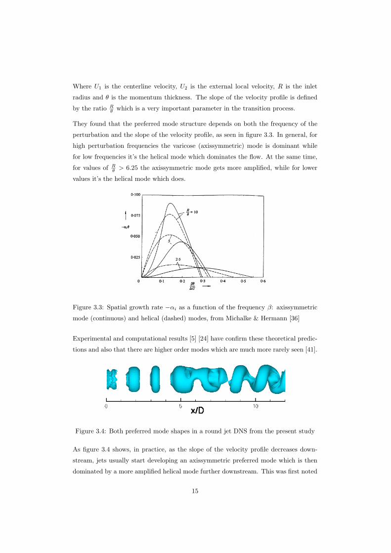
Where U1 is the centerline velocity, U2 is the external local velocity, R is the inlet

radius and θ is the momentum thickness. The slope of the velocity profile is defined

by the ratio Rθ which is a very important parameter in the transition process.

They found that the preferred mode structure depends on both the frequency of the

perturbation and the slope of the velocity profile, as seen in figure 3.3. In general, for

high perturbation frequencies the varicose (axissymmetric) mode is dominant while

for low frequencies it’s the helical mode which dominates the flow. At the same time,

for values of Rθ > 6.25 the axissymmetric mode gets more amplified, while for lower

values it’s the helical mode which does.

Figure 3.3: Spatial growth rate −αi as a function of the frequency β: axissymmetric

mode (continuous) and helical (dashed) modes, from Michalke & Hermann [36]

Experimental and computational results [5] [24] have confirm these theoretical predic-

tions and also that there are higher order modes which are much more rarely seen [41].

Figure 3.4: Both preferred mode shapes in a round jet DNS from the present study

As figure 3.4 shows, in practice, as the slope of the velocity profile decreases down-

stream, jets usually start developing an axissymmetric preferred mode which is then

dominated by a more amplified helical mode further downstream. This was first noted

15

by Crighton & Gaster [6].

Secondary instabilities

After the potential core and once the primary instabilities have established, the axis-

symmetric or helical vortex rings start to suffer an azimuthal instability like the rings

shown in figure 3.5. The wave number n, corresponding to the number of waves along

the circumference of the vortex ring was found by Widnall et al. [47] to respect the

relation:

R/ae = n/k (3.3)

where R is the ring radius, ae is the effective core radius and k is a constant. However,

it was found later by Lim & Nickels [31] that the wave number was not independent

of the Reynolds number and subsequently Saffman [43] refined the relation above

including viscosity effects to correctly predict the variation of this instability length

scale with the Reynolds number.

Figure 3.5: Azimuthal instability in a vortex ring, from Van Dyke [17]

At the same time, in the low vorticity zone between two consecutive vortex rings a

strong stretching mechanism is occurring that concentrates the vorticity in thin sheets

which, induced by the azimuthal instability present, will eventually roll up to form

counter rotating streamwise vortex pairs, structures seen in both experimental [30]

and numerical works [46] [33].

Once these streamwise vortex pairs form, they produce very intense lateral jets ejecting

fluid from the core of the shear layer due to the high radial velocity induced between

them. They also cause an abrupt increase in the entrainment rate due to their mutual

induced radial motion [30].

16

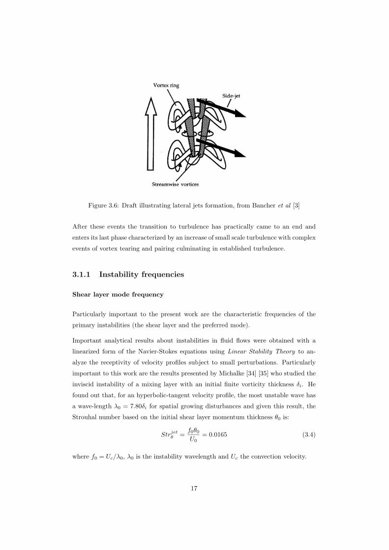
Figure 3.6: Draft illustrating lateral jets formation, from Bancher et al [3]

After these events the transition to turbulence has practically came to an end and

enters its last phase characterized by an increase of small scale turbulence with complex

events of vortex tearing and pairing culminating in established turbulence.

3.1.1 Instability frequencies

Shear layer mode frequency

Particularly important to the present work are the characteristic frequencies of the

primary instabilities (the shear layer and the preferred mode).

Important analytical results about instabilities in fluid flows were obtained with a

linearized form of the Navier-Stokes equations using Linear Stability Theory to an-

alyze the receptivity of velocity profiles subject to small perturbations. Particularly

important to this work are the results presented by Michalke [34] [35] who studied the

inviscid instability of a mixing layer with an initial finite vorticity thickness δi. He

found out that, for an hyperbolic-tangent velocity profile, the most unstable wave has

a wave-length λ0 = 7.80δi for spatial growing disturbances and given this result, the

Strouhal number based on the initial shear layer momentum thickness θ0 is:

Strjetθ =f0θ0U0

= 0.0165 (3.4)

where f0 = Uc/λ0, λ0 is the instability wavelength and Uc the convection velocity.

17

Monkewitz and Huerre [37] generalized the previous case, arriving at a Strouhal num-

ber based on the average velocity U = (U1 + U2)/2:

Strmixθ =f0θ0

U= 0.033 (3.5)

which is the same of the previous case if U1 = U0 and U2 = 0.

There is a good agreement between this linear stability theory and experimental work

[7], [23] and numerical simulations [22], [13].

Preferred mode frequency

As the preferred mode instability occurs towards the end of the jet’s potential core,

where the shear layer is no longer considered thin, curvature effects have to be taken

into account in theoretical studies. This was carried out by [6] who performed a non-

linear stability analysis of jets finding most unstable mode to correspond to a Strouhal

number:

Strjetθ =f1D

U0= 0.4 (3.6)

where D is the jet diameter and f1 the preferred mode frequency of vortex rings at

the end of the potential core. Various experimental [7] and numerical [39], [13] studies

have indeed observed that all jets, for a sufficiently high Reynolds number, present a

Strouhal number between the values: 0.24 < StrD < 0.5.

It has also been experimentally observed that for R/θ0 < 120 the Shear layer and Pre-

ferred Strouhal numbers are proportional, while from that value on the latter Strouhal

number locks at the constant value of StrD = 0.44, but a good explanation for this

has yet to be found.

3.2 Unsteady Jets

There’s been so little research in this subject that it is very difficult to leave any of

the previous works out of this state of the art discussion.

The first published work on unsteady jets came from Kato et al. [26] in 1986. They

proposed that an unsteady jet could modify the mixing rate i.e. altering the ratio

of ambient to nozzle fluid ingested into turbulent vortices by means of the present

unsteady effects.

18

Their start hypotheses was: If the inlet flow is continuously accelerated then the vortex

engulfment appetite is completely satisfied by this stream and negligible ambient fluid

will be entrained, dramatically reducing the mixing capability of the jet.

Their experiment consisted of a linearly accelerated jet of around ReD = 104 in a

water tank and using pH indicators they observed a 25% lengthier and 50% wider jet

flame.

It was also argued that to maintain most of the unsteady effects the jet had to be

accelerated at an exponential rate, otherwise (if for example it was accelerated at a

linear rate) the jet would return to a quasi-steady behavior, even though the jet was

still accelerating.

Later in 1986, Breidenthal [4] postulated the turbulent exponential jet as a self-

similar flow. He started noticing that all known self-similar flows exhibit Ω(T ) ∼U(T )/X(T ) ∼ 1/T meaning that the vorticity of each structure depends only on their

age. Capital letters are Lagrangian quantities.

He continues, stating that in a nonsteady flow with characteristic time scale τ the

vorticity of a given structure can be independent of its age, Ω = (1/τ)f(t0/τ) and that

to keep vorticity to decline downstream then f must be the exponential f(t0/τ) =

et0/τ :

Ω = (1/τ)et0/τ (3.7)

Then U(T ) and X(T ) can be obtained through:

U(T ) =dX(T )dT

∼ ΩX(T ) (3.8)

resulting in:

Ω = (1/τ)et0/τ (3.9)

X(T ) = λe(T/τ)et0/τ (3.10)

U(T ) = (λ/τ)et0/τe(T/τ)et0/τ (3.11)

In early 1993 Kouros et al. [27] performed experiments in a gravity driven (accel and

decelerated) ReD ≈ 104 jet. They found the jet’s spreading rate to be less than half of

the equivalent steady jet’s, contrary to previous observations on unsteady jets (includ-

ing pulsed jets). Furthermore, a large symmetric starting vortex was observed, which

would separate from the flow further downstream, presumably due to deceleration of

the jet after the initial acceleration.

19

Later in 1993 Roy & Johari [42] performed the first numerical simulations of a linear

accelerated jet. He used an algebraic eddy viscosity model of turbulence in a finite

element method to study the unsteady jet’s entrainment. In order to compare both the

steady and unsteady jet’s entrainment characteristics they proposed a new normalized

entrainment quantity:

E∗ =∫u(x, r, t)rdr

uc(x=0,t)uc(x=0,t=0)

∫u(x, r, t = 0)rdr

(3.12)

where uc is the centerline velocity.

Results showed an unsteady jet with reduced entrainment (see figure 3.7) and also an

advecting arrow shape front separating the steady from the unsteady jet.

Figure 3.7: Normalized entrainment from Roy & Johari computational results [42]

In 1996 Zhang & Johari [50] presented some new discoveries following their experi-

mental work on linearly, quadratically and exponentially accelerated jets.

They observed a big concentration dye front, advecting much faster than the previ-

ously established steady jet turbulent structures and additionally to this a decreased

spreading rate after the passage of this front (see the pictures on figure 3.8) from which

they also concluded that the entrainment rate decreased during acceleration, because

in the steady jet the spreading rate is proportional to the entrainment rate.

From their results and discussion, they hypothesize that the unsteady effects are only

present in the vicinity of the front and that upstream of it the jet had relaxed back to

a quasi-steady state with small acceleration effects.

Furthermore, they rule out the influence of the Reynolds number and acceleration rate

in their observations.

In 1997, Johari & Paduano [25] experimented in a gravity driven jet (deceleration after

initial acceleration) and found that the decelerating jet dilutes more (more entrain-

ment) than the classic steady jet.

20

a) b)

c) d)

Figure 3.8: Concentration front on experiment by Zhang & Johari [50]

More than 10 years had to pass before Abani & Reitz [1] revisited the subject. They

proposed a new model for the jet tip penetration of unsteady turbulent round jets and

performed experiments with 13 different transient injection profiles to validate it.

3.3 Vortex Rings

3.3.1 Helmholtz theory

Abani & Reitz’s jet tip penetration model [1] was built using results from the Helmholtz

vortex motion theory for a moving isolated ring. Figure 3.9 is a sketch of the approx-

imate evolution of vortex rings in a round jet:

Figure 3.9: Aproximate sketch of the vortex rings in a round jet, from Abani & Reitz [1]

According to Helmholtz’s second vortex theorem, the convection velocity for a vortex

ring, Uv is of the order of:

Uv ∼ Γδ

(3.13)

and the circulation Γ for all cross sections of a given vortex ring is independent of

21

time:

Γ(x) =4U(x)δπ

(3.14)

where Γ(x) is the circulation of a ring at a given downstream location x at which the

centerline velocity is U(x).

Hence, the vortex ring keeps its circulation as it travels, equal to when it was generated:

Γ(x) = Γinj =2UinjD

π∼ UinjD (3.15)

where the inj subscript indicates values at the time of injection and D is the nozzle

diameter.

3.3.2 Vorticity wake

Another relevant feature is the existence of a vorticy wake behind a traveling vortex

ring. This was first postulated by Maxworthy [32] and was later experimentally and

numerically confirmed.

Figure 3.10 shows the vorticity wake of a vortex ring visible by vorticity patches

over instantaneous streamlines for an isolated vortex ring. The figure is from an

experimental work on isolated vortex rings by Dabiri & Gharib [12]. The streamlines

are from a vortex ring frame of reference.

Figure 3.10: Instantaneous streamlines and vorticity patches (vortex ring frame of

reference), from Dabiri & Gharib [12]

22

Chapter 4

Numerical Method

The simulations reported in this work are simulations of incompressible flows of New-

tonian fluids in an inertial frame of reference. The numerical code used, was developed

by Gonze [21], is called SPECOMPACT and uses a pseudo-spectral scheme and a high

order compact scheme to solve the unsteady, incompressible Navier-Stokes equations,

which provide an exact description of the problem.

It has been extensively validated by da Silva et al. [9] and da Silva & Metais [10] [11],

in simulations of round, plane and coaxial jets. An extensive description of the code

is available at [8].

4.1 Governing Equations

The differential system of equations to be solved is written as (in cartesian coordinates):

• Linear momentum transport equations

∂ui∂t

+ uj∂ui∂xj

= −1ρ

∂p

∂xi+ ν

∂2ui∂x2

j

+ fi (4.1)

• Mass conservation equation

∂ui∂xi

= 0 (4.2)

23

where t is the time, xi are the cartezian coordinates, ui are the velocity components

along those coordinates, p is the pressure, ρ is the density, ν the kinematic viscosity

and fi are the external body forces inexistent in this work.

4.2 Code Philosophy

The code was developed with the spatial simulation approach. This means the com-

putational domain was build in a region of interest (in this case at the inlet of a round

jet) and the flow enters and leaves this stationary box. This is the type of simulation

better fit (more physically realistic) for the simulation of turbulent round jets as it

allows for pressure feedback from downstream to upstream locations, essential in a

transition process, which is not allowed in the temporal simulation approach because

of it’s need for periodic streamwise boundary conditions.

4.2.1 Computational box

The computational domain consists of a parallelepiped of lengths Lx, Ly and Lz, x

being the streamwise, y the normal and z the spanwise directions, respectively.

At the center of the inlet plane (x = 0) is the jet inlet of diameter D.

The box dimensions are 12D x 7.5D x 7.5D and it’s discretized with a mesh with 201

x 128 x 128 points in each of the above directions, respectively.

4.3 Numerical Solver

4.3.1 Spatial discretization

Pseudo-spectral schemes

To use a pseudo-spectral scheme is to solve the discretized equations in the Fourier

space instead of the physical space. Advantages of this scheme are its high accuracy

and low computational cost, but it requires periodic boundary conditions and that is

a disadvantage.

24

This code uses these schemes to solve the equations in the lateral directions. So, any

given flow variable φ(x, y, z, t) is periodic along the normal y and spanwise z directions

and can be expanded using an inverse 2D discrete Fourier transform:

φ(x, y, z, t) =

ny2 −1∑

j=−ny2

nz2 −1∑

k=−nz2φ(x, ky, kz, t)eι(kyy+kzz) (4.3)

where ky and kz are the Fourier wave numbers,

ky =2πLyj (4.4)

kz =2πLzk (4.5)

Ly and Lz are the lateral lengths of the computational box, ny and nz are the number

of discretization points along the lateral directions, and ι =√−1 is the imaginary

unit.

The direct 2D discrete Fourier transform gives each Fourier coefficient φ:

φ(x, ky, kz, t) =1

nynz

ny−1∑j=0

nz−1∑k=0

φ(x, y, z, t)e−ι(kyy+kzz) (4.6)

The derivatives in the physical space are instead multiplications in the Fourier space:

∂φ

∂y= ιkyφ (4.7)

∂φ

∂z= ιkzφ (4.8)

Compact schemes

Compact schemes are finite differencing schemes which involve not only neighbor points

but also derivatives in the neighbor points, in an implicit way.

Pade proposed a scheme involving f , fi+1 and fi−1 and also f ′, f ′i+1 and f ′i−1:

f ′j + a3f′j+1 + a4f

′j−1 = a0fj + a1fj+1 + a2fj−1 (4.9)

which results in a system of equations in the form of a tri-diagonal matrix that can

be quickly solved to get the derivative f ′j at each point in a given direction. This is

known as the Pade approximation.

25

[29] presented Pade approximations for the 1st and 2nd derivatives up to the 10th

order of accuracy in the form:

β(φ′x)i−2 + α(φ′x)i−1 + (φ′x)i + α(φ′x)i+1 + β(φ′x)i+2 =

cφi+3 − φi−3

6h+ b

φi+2 − φi−2

4h+ a

φi+1 − φi−1

6h(4.10)

The coefficients for 6th order accuracy used in this code for the first and second deriva-

tive are:

derivative α β a b c

1st 13 0 3

2 (α+ 2) 14 (4α− 1) 0

2nd 211 0 12

11311 0

An high accuracy order is very important in this kind of simulations because the higher

the accuracy of the scheme, the higher wave number functions it is able to correctly

calculate the derivative of. This is crucial to get the small scales of turbulence.

4.3.2 Temporal advancement

The code uses a three step, 3rd order Runge-Kutta time stepping scheme to compute

each new velocity at the new sub-step ~uk ≡ ~un+1 from the last two sub-steps ~uk−1

and ~uk−2 ≡ ~un.

~uk − ~uk−1

∆t= αk

[N(~uk−1

)+ L

(~uk−1

)]+ βk

[N(~uk−2

)+ L

(~uk−2

)]+ ~∇pk (4.11)

~∇.~uk = 0 (4.12)

The coefficients αk and βk for 3rd order accuracy are [48]:

α1 =815

β1 = 0

α2 =512

β2 = −1760

α3 =34

β3 = − 512

(4.13)

4.3.3 Pressure-velocity coupling

In order to solve equation 4.11 the pressure field p has to be known at each substep

and the mass conservation equation 4.12 has to be respected because the flow is in-

compressible. The pressure field role is to enforce this incompressibility condition on

26

the velocity field, making equations 4.11 and 4.12 strongly coupled. Because of this

reason they have to be solved simultaneously.

This code tackles this problem by solving a Poisson equation for the pressure at each

sub-step of the time stepping scheme.

Inside each sub-step a intermediate velocity field ~u∗ is calculated by:

~u∗ − ~uk−1

∆t= αk

[N(~uk−1

)+ L

(~uk−1

)]+ βk

[N(~uk−2

)+ L

(~uk−2

)](4.14)

and the pressure field at the end of the substep k has to verify:

~uk − ~u∗∆t

= −~∇pk (4.15)

Applying divergence to this equation one arrives at:

~∇.~uk − ~∇.~u∗∆t

= −∇2pk (4.16)

which, with 4.12, leads to the Poisson equation:

∇2pk =~∇.~u∗∆t

(4.17)

Once solved, the the pressure field at the end of the sub-step k is known and the

velocity field ~up is obtained from 4.16.

The Poisson equation is discretized using the spatial discretization schemes previously

described.

4.3.4 LES sub-grid scale model

In addition to the numerical solver parts just described and as already discussed in

section 2.3, the DNS approach is not possible at high Reynolds numbers.

When this is the case (it is in some simulations in the present work) the smallest scales

of the flow are smaller than the mesh used. The mesh is then functioning as an implicit

filter, explicitly solving only the larger scales of the flow. It is then needed to use a

Sub-Grid Scale (SGS) model.

Here the Filtered structure function model (Ducros et al. [16]) is used.

27

4.4 Boundary Conditions

4.4.1 Lateral boundaries

Since the code uses pseudo-spectral schemes in the lateral directions for a maximum

possible order of accuracy, the lateral boundaries of the computational domain have

to be periodic. This means that:

~u(x, y, z, t) = ~u(x, y + Ly, z, t) (4.18)

~p(x, y, z, t) = ~u(x, y + Ly, z, t) (4.19)

~u(x, y, z, t) = ~u(x, y, z + Lz, t) (4.20)

~p(x, y, z, t) = ~u(x, y, z + Lz, t) (4.21)

Note that these do not require the instantaneous velocities normal to the lateral bound-

aries to be zero. They require the mean to be zero.

In practice this means that this code simulates an infinite array of round jets, instead

of an isolated one, creating a problem of jet growth by entrainment, since in the mean

there is no fluid entering the computational box in the directions normal to the lateral

boundaries.

In order to tackle this problem, [15] and [44] shown that to make the simulated jet dy-

namics similar to those of a free jet the lateral boundaries have to be placed sufficiently

far away and a small positive co-flow has to be added to the inlet boundary.

If this positive co-flow is very small, it doesn’t affect the flow’s stability characteristics

but allows for the natural growth of the jet by entrainment. There is a very good

agreement with experimental measurements.

4.4.2 Inlet condition

The inlet condition consists of a prescribed inlet velocity field at each time step with

the form (in polar coordinates):

~U(r, t) = ~Umed(r, t) + ~Unoise(r, t) + ~Uforc(r, t) (4.22)

Where ~U(r, t) is the instantaneous inlet velocity vector and ~Umed(r, t) is the mean

streamwise velocity profile which evolves in time only during acceleration.

28

To mimic the inlet velocity profile found experimentally in round jets [18] an hyperbolic

- tangent profile [36] was used as it is known to be a good approximation of real inlet

velocity profiles:

~Umed(r, t) =U1(t) + U2

2− U1(t)− U2

2tanh

[14R

θ0

(r

R− R

r

)]· ~ex (4.23)

Where U1(t) is the jet centerline velocity, U2 is the small co-flow discussed above, θ0

is the momentum thickness of the initial shear layer and R = D/2.

~Unoise is the noise profile given by:

~Unoise = AnUbase(r)~f ′ · ~ex (4.24)

Where An is the maximum noise amplitude and Ubase is a function used to concentrate

the noise mostly at the shear layer gradients:

Ubase(r) =

1 if 0.8 < r/D < 1.2

0.2 if r/D < 0.8

0 otherwise

f ′ is a tri-dimentional random noise designed to satisfy a given energy spectrum:

E(k) = ks exp[−s2

(k/k0)2] (4.25)

Where k = (k2y + k2

z)1/2 is the wave number norm in the (y, z) plane.

The exponent s and the peak wave number k0 were chosen to simulate an energy input

at small scales, hence high k0, and a large-scale spectral behavior found in decaying

isotropic turbulence (s <= 4).

This numerical noise is necessary to allow for a natural transition of the jet. Though it

is essentially white noise, the flow will naturally choose which are the most amplified

modes during the transition process, like previously discussed in the transition to

turbulence introduction in chapter 2.

The ~Uforc component of the inlet velocity condition is used to amplify the initial

coherent structures of the transition process for better visualization and easier post-

processing of the results.

It consists of a sinusoidal signal with the same frequency of the jet’s preferred mode,

directly added to the mean velocity inlet profile ~Umed:

~Uforc(r, t) = εUxmed(r, t) sin(

2πStrDU1t

D

)· ~ex (4.26)

29

This excitation is equivalent to what is done experimentally with loudspeakers, in

studies of forced jets and is sketched in figure 4.1.

Figure 4.1: Sketch of the Uforc component in the inlet profile, from Urbin & Metais [45]

4.4.3 Outlet condition

This boundary condition is usually the one that poses the most difficulty. Since this is a

spatial simulation the flow must leave the computational box without any perturbation

from the outlet boundary, which is quite hard to completely achieve.

This code implements a non-reflective outflow condition [40] used in a way which

does not disturb the pressure-velocity coupling. It starts with a modified form of the

Navier-Stokes momentum equation for the streamwise direction:

∂u

∂t= −Cu(y, z)

∂u

∂x− v ∂u

∂y− w ∂u

∂w+

1Re

(∂2

∂y2+

∂2

∂z2

)u (4.27)

where Cu(y, z) includes the effects of longitudinal pressure gradient ∂p∂x , dissipation

1Re

∂2u∂x2 and convective Cu(y, z)∂u∂x terms.

This equation is used to compute Cu(y, z) at i = nx − 1 in each sub-step of the

Runge-Kutta time advancing scheme:

~uk − ~uk−1

∆t= −Cu(y, z)

∂u

∂x− v ∂u

∂y− w ∂u

∂w+

1Re

(∂2

∂y2+

∂2

∂z2

)u (4.28)

and then used again at i = nx to compute the streamwise velocity at the outlet,

because Cu(y, z) is already known.

Then the Poisson equation is solved and the normal and spanwise velocities v and w

30

are corrected at i = nx ending the sub-step procedure:

vnx(y, z) = v∗nx(y, z)− ∂p

∂y(4.29)

wnx(y, z) = w∗nx(y, z)− ∂p

∂z(4.30)

It was observed by Gonze [21] and da Silva [8] that the turbulent coherent structures

leave the computational domain without distortion.

31

Chapter 5

Linear Acceleration of

Turbulent Round Jets

This chapter presents the core of this work on acceleration of round jets. It starts with

an overview of all the simulations performed and continues with a detailed discussion

of all the results, divided in three main sections devoted to: kinematics of the vortex

motion, topology of the vortex rings and jet entrainment.

5.1 Simulations

Seventeen simulations of linearly accelerated round jets were performed corresponding

to about 24 weeks of total processor time at LASEF - Laboratory and Simulation of

Energy and Fluids, Instituto Superior Tecnico, Portugal.

Two other simulations were performed, corresponding to decelerated jets, but after an

initial post-processing, research on that issue was halted as it would literally double the

amount of work. The preliminary results will be presented at the end of this chapter

but it will be left as an open matter for future research.

All the accelerated jet simulations consisted of 3 phases, beginning with the initial

steady jet at a given Reynolds number ReiD, followed by the acceleration phase which

lasted until the Reynolds number has doubled to RefD = 2ReiD, reaching the third and

final phase of constant Reynolds.

32

The acceleration was produced by increasing the mean inlet velocity profile linearly in

time:~Umed(r, t) = ~Umed(r, t = 0) · (1 + αt) (5.1)

where α is the acceleration rate. The acceleration profiles for some simulations with

different acceleration rates is shown in figure 5.1:

Figure 5.1: Inlet Reynolds number ReD evolution for some simulations

Three main parameter changes were studied: the acceleration rate, the Reynolds num-

ber and the presence of the inlet forcing component Uforc. There was no need to

perform all the permutations between these, so, a base simulation point was chosen

regarding the acceleration rate and Reynolds number, with α = 0.06 and ReiD = 500.

These base parameter values were chosen because they allow for a good acceleration

time (it is a low acceleration rate) and also for a slow enough transition to turbulence,

needed for a good visualization of the processes’ turbulent coherent structures.

From this base simulation two branches have parted: First the acceleration rate was

changed in the range between α = 0.02 and α = 0.6 with a fixed initial Reynolds

number ReiD = 500.

Then, the Reynolds number was also changed between ReiD = 500 and ReiD = 10000

for a fixed acceleration rate of α = 0.06.

Added to this, some selected simulation points were performed with and without the

inlet forcing component Uforc.

33

Table 5.1 resumes the information just discussed.

ReiD => RefD

α ∆t∗ 500 => 1000 1000 => 2000 10000 => 20000

0.02 40-90 x

0.04 40-65 x o

0.06 40-57 x o x o X O

0.08 40-53 x

0.1 40-50 x

0.2 40-45 x

0.4 40-43 x

0.6 40-41 x o

−0.06 40-57 x ox : DNS with Uforc o : DNS without Uforc

X : LES with Uforc O : LES without Uforc

Table 5.1: Simulations of accelerated jets performed throughout this work

Since the computational mesh was always the same 201 x 128 x 128 box it would not

be possible to perform the Direct Numerical Simulations of the ReD = 10000 cases

because the smallest scales of turbulence, of the order of the Kolmogorov scale η are,

at this Reynolds number, smaller than the mesh’s characteristic length, as discussed in

section 2.1. So, these high initial Reynolds number simulations are instead Large-Eddy

Simulations.

5.2 Overview of the Base Simulation

The first and base simulation performed had an initial Reynolds number of ReiD = 500,

accelerating to RefD = 1000 with an acceleration rate of α = 0.06.

Initial post-processing consisted of visualization of the coherent structures by means

of the positive Q criteria.

It could have been done by means of the pressure or vorticity fields, but using the Q

quantity field enhances the quality of the visualization. This quantity is defined as the

34

second invariant of the velocity gradient tensor:

Q =12

(ΩijΩij − SijSij) (5.2)

where Ωij = 12

(∂ui∂xj− ∂uj

∂xi

)and Sij = 1

2

(∂ui∂xj

+ ∂uj∂xi

)So, it defines regions of both high local vorticity and low rate of deformation, ideal for

visualization of the primary coherent structures of the jet.

Figure 5.2: Centerline slice with contour of Q > 0.01 prior to the acceleration

As expected, post-processing revealed an initial steady jet where the vortex rings were

being shed with a frequency which corresponded to a Strouhal number StrD = 0.375

of the preferred mode as seen in figures 5.2. At this relatively low Reynolds number

the primary coherent structures of turbulence are not unstable and turbulence does

not develop. Instead, the initial vortex rings are seen to fade towards the end of the

computational box.

However, as the jet starts to accelerate, a non-linear change of the shear layer mode

frequency was apparent. The primary Kelvin-Helmholtz vortex rings were now shed

with a much higher frequency than the preferred mode frequency.

Figures 5.3 and 5.4 show iso-surfaces of positive Q and contours of Q, respectively, a

short while into the acceleration phase. The vortex rings shed prior to the acceleration

are still inside the computational box. These are the four rings visible on the right

of the figures. The four smaller vortex rings on the left were already shed during the

acceleration phase.

As the jet continues to accelerate (figure 5.5, and as a consequence of it, several merging

events happen to this phase’s smaller vortex rings until around x/D = 6. Downstream

of this location there were no apparent differences between the steady and unsteady

35

Figure 5.3: Iso-surfaces of positive Q

Figure 5.4: Centerline slice with contour of Q > 0.01 during the acceleration

36

phases of the simulation except for the fact that now the vortex rings do not fade away

towards the end of the computational domain. Still no signs of secondary instabilities

are present.

Figure 5.5: Centerline slice with contour of Q > 0.01 at the end of acceleration

After the acceleration had ceased (figure 5.6) the flow quickly returned to the well

known steady state. Now the vortex rings are being shed at the preferred mode

frequency. Additionally, at this Reynolds number, the transition to turbulence is

mostly visible inside the computational domain, including the azimuthal instability

and streamwise vortices.

Figure 5.6: Centerline slice with contour of Q > 0.01 after the acceleration

Influence of inlet forcing component Uforc

Since the first simulation was performed using the amplification inlet forcing previously

discussed, it was necessary to perform a second simulation without this forcing, in order

to check its influence on the jet during the acceleration.

37

With Uforc = 0 the jet’s coherent structures appeared less intense but qualitatively

all remained the same.

Further investigation of the effects of the Uforc influence was done via spectra of

the y component of the velocity field. The results confirm that although the Uforc

component does amplify the jet’s coherent structures during its steady phases, it has

virtually no influence during the acceleration phase (see figure 5.7). In fact, because

the primary structures’ shedding frequency is no longer correspondent to an equivalent

Reynolds steady jet, the forcing component becomes irrelevant during acceleration.

Figure 5.7: Spectra of v during acceleration with and without the Uforc component.

This means that the forcing component can be used for enhanced visualizations when-

ever needed, or left disabled for calculation of other quantities which are more accurate

without it.

From this point on the study could concentrate on the physical aspects of the flow,

given that the non-linear effects during acceleration were not the result of a numerical

artifact.

38

5.3 Kinematics of the Vortex Motion

5.3.1 Acceleration maps

Along with two and three dimension visualization with the Q criteria other forms of

post-processing were used in order to permit a more detailed study of the kinematics

of this particular flow.

Acceleration maps were developed, consisting of a positive Q contour plotted in a

t∗ = t(U1(0)/D) vs x∗ = x/D graph that presents the streamwise evolution of each

vortex ring’s position.

Shown in figure 5.8 is the gradient zone (30 < t∗ < 70) of an acceleration map corre-

sponding to the α = 0.06 and ReiD = 500 simulation.

Figure 5.8: Acceleration map of the base simulation, α = 0.06, ReiD = 500

These acceleration maps are records of the whole simulations, where it is possible to

track each vortex ring and analyze the different phases and zones, including the vortex

merging events during the acceleration phase.

Figure 5.9 features the acceleration maps of selected simulations with different acceler-

39

ation rates, from α = 0.06 to α = 0.2 all with ReiD = 500 with the forcing component.

ReiD = 500

Figure 5.9: Acceleration maps

Based on these acceleration maps, each vortex ring trajectory can be isolated in order

to allow for calculation of the actual vortex shedding frequency. Each vortex ring’s

local convection velocity may also be computed from these trajectory maps by taking

the slope of each trajectory v∗c = ∂x∗/∂t∗.

5.3.2 Influence of the Reynolds number

The next step was to verify that the non-linear effects were not solely due to the

Reynold number ReiD = 500 at which the simulation was carried out. So, still at the

same acceleration rate α = 0.06 the influence of the Reynolds number was studied in

40

various simulations with starting Reynolds number of ReiD = 1000 and ReiD = 10000.

Comparison of the different simulations showed that the non-linear effect is present

regardless of the Reynolds number at which the simulation starts.

Figure 5.10: Acceleration map for α = 0.06, ReiD = 1000

In fact, analysis of the acceleration maps of both the α = 0.06 simulations, at Re = 500

and Re = 1000 (figures 5.8 and 5.10) reveals very few differences between them. Not

only the non-linear effect is present during the acceleration phase, but also the size

and streamwise evolution (life) of each vortex ring is identical in both simulations.

5.3.3 Vortex ring merging events

The three different phases of each simulation are clearly visible in the acceleration

maps. In the initial steady phase the vortex rings travel with approximately constant

speed as they also do in the final steady phase, but faster in the latter, this translates

to an higher trajectory slope in the maps. During acceleration the smaller and higher

frequency primary vortex rings are also visible along with a series of merging events

that do not take place during the steady phases.

41

Figure 5.11: Acceleration map of the base simulation, α = 0.06, ReiD = 500

Moreover, the zone in the acceleration map of the base simulation (in figure 5.11)

corresponding to the acceleration phase can also be divided in three different regions.

The first, x/D < 4 where most of the primary merging events take place, the second,

4 < x/D < 8 where only a few secondary merging events happen and the third and

last region, x/D > 8 where there are no merging events. These regions were named

A, B and C, respectively. Furthermore, hA was defined as the length of zone A, it

represents the mean location of the primary mergings.

After all the simulations were performed and their acceleration maps were available,

the length of zone A was evaluated to build figure 5.12.

Additionally, the number of primary (zone A) and secondary (zone B) merging events

was also evaluated to form figure 5.13:

As visible in the acceleration maps of figure 5.9 and table A.5, the length hA decreases

as the acceleration rate increases to the point that when α = 0.4 it is no longer visible

in the maps because the acceleration phase is too fast.

42

Figure 5.12: Height of zone A for each simulation

Figure 5.13: Number of primary (A) and secondary (B) merging events

43

5.3.4 Characteristic frequencies

Shear layer mode frequency

As already discussed, the frequency of the primary vortex rings can be computed via

the acceleration maps.

Figure 5.14 shows once more that the Reynolds number has no influence in the de-

velopment of the non linear effects during the acceleration. It features the computed

frequency of the primary vortex rings for the ReiD = 500 and ReiD = 1000 simulations,

and shows that apart from some twitches resulting from the increased difficulty to

compute the frequency at a higher Reynolds number, there is no difference between

the two simulations.

Figure 5.14: Influence of the Reynolds number in the vortex shedding frequency for

α = 0.06

Figure 5.15 shows the shear layer mode frequency for simulations with different α at

the same ReD = 500. It clearly shows that during the acceleration phase the shedding

frequency is much higher than during the steady phases. Moreover, it also shows that

as the acceleration rate α increases, so does the mean vortex ring shedding frequency

during the acceleration phase. In fact their relation is very close to linear, as shown

in figure 5.16.

44

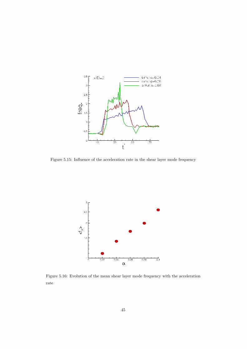
Figure 5.15: Influence of the acceleration rate in the shear layer mode frequency

Figure 5.16: Evolution of the mean shear layer mode frequency with the acceleration

rate

45

Preferred mode frequency

The preferred mode was considered to be present after the last merging has happened.

More striking than its frequency, which changes almost linearly during acceleration,

is the fact that as the acceleration progressed, the last merging would occur further

downstream, meaning that the preferred mode was established much later. At first at

around x/D = 3 and at around x/D = 9 at the end of the unsteady phase. This is

shown in the acceleration map of the base simulation, and also in the map correspond-

ing to the ReiD = 1000 simulation, figures 5.8 and 5.10, respectively.

46

5.4 Topology of the Vortex Rings

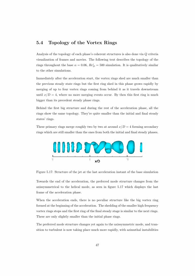
Analysis of the topology of each phase’s coherent structures is also done via Q criteria

visualization of frames and movies. The following text describes the topology of the

rings throughout the base α = 0.06, ReiD = 500 simulation. It is qualitatively similar

to the other simulations.

Immediately after the acceleration start, the vortex rings shed are much smaller than

the previous steady state rings but the first ring shed in this phase grows rapidly by

merging of up to four vortex rings coming from behind it as it travels downstream

until x/D = 4, where no more merging events occur. By then this first ring is much

bigger than its precedent steady phase rings.

Behind the first big structure and during the rest of the acceleration phase, all the

rings show the same topology. They’re quite smaller than the initial and final steady

states’ rings.

These primary rings merge roughly two by two at around x/D = 4 forming secondary

rings which are still smaller than the ones from both the initial and final steady phases.

Figure 5.17: Structure of the jet at the last acceleration instant of the base simulation

Towards the end of the acceleration, the preferred mode structure changes from the

axissymmetrical to the helical mode, as seen in figure 5.17 which displays the last

frame of the acceleration phase.

When the acceleration ends, there is no peculiar structure like the big vortex ring

formed at the beginning of the acceleration. The shedding of the smaller high frequency

vortex rings stops and the first ring of the final steady stage is similar to the next rings.

These are only slightly smaller than the initial phase rings.

The preferred mode structure changes yet again to the axissymmetric mode, and tran-

sition to turbulent is now taking place much more rapidly, with azimuthal instabilities

47

Figure 5.18: Structure of the jet at the final steady stage

and streamwise vortices all present inside the computational domain, as can be seen

in figure 5.18.

Figure 5.19’s three figures respectively illustrate the main differences between the three

different phases’ typical primary vortex rings.

Aside from the size of the vortex rings during each phase there is another visible feature

in the figures of figure 5.19, small wakes behind the vortex rings of the steady stages

(first and third figure) and also another small wake in front of the smaller vortex ring

of the acceleration phase.

To further study the downstream topological evolution of the vortex rings two quan-

tities were computed, Er and Eθ:

Er(x) =

√1

LyLz(2π

∫〈u′2r (x, r)〉rdr) (5.3)

Eθ(x) =

√1

LyLz(2π

∫〈u′2θ (x, r)〉rdr) (5.4)

These quantities represent the contribution of the radial and azimuthal Reynolds

stresses contribution to the turbulent kinetic energy at a given streamwise plane, hence,

higher values of these quantities represent the departure from the perfect toroidal ge-

ometry of the vortex rings.

As much of the previously discussed quantities, the temporal evolution of these profiles

is non-linear. Both Eθ and Er plots show that these quantities start at a low value

which is maintained during all of the acceleration phase, immediately after which they

considerably rise to much higher values, as seen in figures 5.20 and 5.21:

48

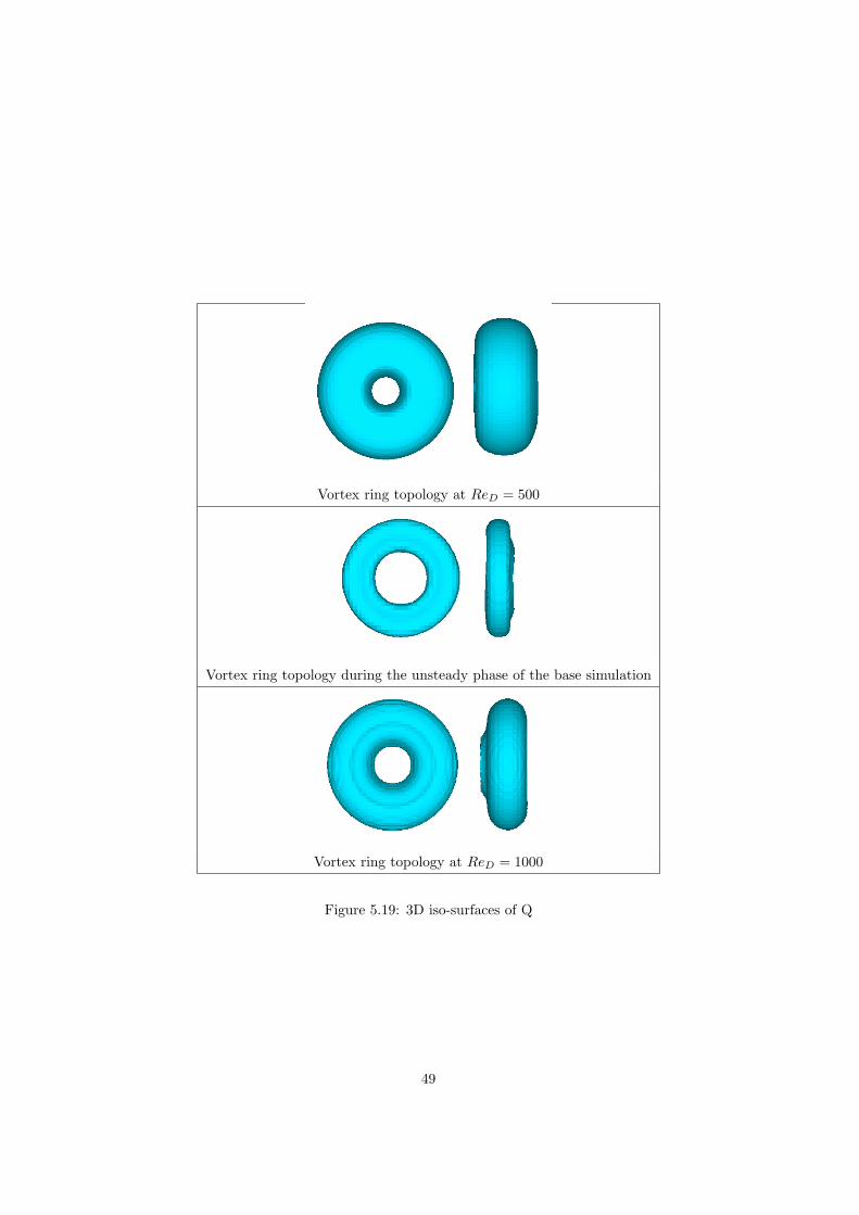
Vortex ring topology at ReD = 500

Vortex ring topology during the unsteady phase of the base simulation

Vortex ring topology at ReD = 1000

Figure 5.19: 3D iso-surfaces of Q

49

Figure 5.20: Temporal evolution of the streamwise profile of Er

Figure 5.21: Temporal evolution of the streamwise profile of Eθ

50

5.4.1 Influence of the acceleration rate

Visible in the acceleration maps of simulations with different acceleration rates in

figure 5.9 and table A.5 is the influence of the acceleration rate in the topology of the

primary vortex rings shed during the acceleration phase.

As the acceleration rate increases and the acceleration time decreases, from simulation

to simulation, the size difference between the steady and unsteady phases’ vortex rings

increases, i.e. the unsteady vortex rings are smaller for high acceleration rates.

51

5.5 Jet Entrainment

Jet entrainment is a very important issue because it is probably the most important

quantity from an application point of view. For the same reason it has been the main

target of the previous studies on unsteady round jets which have always found it to

decrease during acceleration.

5.5.1 Jet width - δ0.5

Rather than the entrainment itself, previous experimental studies have relied on mea-

suring the jet’s half-width as a measure of entrainment, hence this was the first variable

studied and compared with previously available results.

Figure 5.22: Evolution of the δ0.5 profile for α = 0.02

Figure 5.22 shows the calculated jet half width for the α = 0.02 simulation. It is clearly

visible that, in accordance with previous results, it decreases as the jet accelerates.

Analysis of the same variable for different simulations also showed that the jet’s half

width decreases as the acceleration rate increases, for the same instant t∗. see figure

5.23.

As for an unsteady jet there is not a clear link between the jet’s half width and the jet’s

entrainment, and even though jet width measurements confirmed that it ”shrinks”

during the acceleration phase, previous insights into the jet’s coherent structures’

52

Figure 5.23: δ0.5 at a given time for several α’s

kinematics and topology hinted that the entrainment could still be increasing during

the unsteady phase.

5.5.2 Streamwise mass flow rate

To directly study the entrainment rate the obvious choice would be to compute the

streamwise evolution of the jet’s mass flow rate at each time step but this posed

a problem: the inlet mass flow changes during the unsteady phase and it makes it

impossible to compare the mass flow rate at different times.

The solution was to normalize the mass flow rate, calculating Q∗(x, t) = Q(x,t)Qinlet(x0,t)

as

Roy & Johari [42] did in their computational study on accelerated round jets.

Results for Q∗ (figure 5.24) were in accordance with their work [42] but still left doubt

about the right way to calculate the entrainment rate.

The calculation of Q∗ poses yet another problem. When at a given time t∗acceleratingthe streamwise evolution of Q is calculated and then divided by Qinlet the Q values at

the end of the computational box are being normalized with a Qinlet which is much

higher than the one present when that portion of the flow was being injected in the

computational box. That could not be giving the correct idea of what was indeed

going on regarding the entrainment rate.

53

Figure 5.24: Streamwise evolution of Q∗ at different stages of the base simulation

5.5.3 Radial velocity - Shear layer interface

Leaving the mass flow rate calculations aside, the next step consisted on the evaluation

of the jet’s radial velocity profile as it is also directly related to the entrainment rate.

Figure 5.25 shows radial velocity profiles for the α = 0.06 simulation at x/D = 4 for

the three different simulation phases.

It is clearly seen that it is during the acceleration phase that vr presents its lower

values. This is not enough to conclude about the entrainment rate because the jet’s

half width does not stay constant during the three simulation stages.

In order to tackle these difficulties it was decided to calculate the entrainment rate

directly in the jet’s shear layer interface. At each streamwise coordinate, this interface

was defined as the radial position of the lower vr and then used to calculate the

entrainment rate, defined by:

E(x) =∫ 2π

0

vr(x, θ)rvrdθ (5.5)

Then, time averages of each of the acceleration phases were calculated from each

time step entrainment results in order to have a good picture of the entrainment

characteristics of each phase.

Figure 5.26, corresponding to the entrainment profile of the base simulation, shows

decreasing profiles for both the initial and unsteady phases, consistent with the pre-

54

Figure 5.25: Radial velocity profiles at different stages of the base simulation

viously observed fact that in the base simulation the initial turbulent structures were

not unstable through these phases. Although, still regarding these initial and unsteady

phases of the base simulation, there are local increases in the entrainment rate, for

example at x/D ≈ 9 for both profiles or at at x/D ≈ 5 for the unsteady phase profile.

These localized peaks correspond to mergings (for x/D ≤ 6, i.e. inside the potential

core) or instabilities (further downstream) taking place at the same location through-

out each phase. The peaks at the end of the computational box come from the outlet

boundary condition and should not be considered.

Still observing figure 5.26, the entrainment profile of the last steady ReD = 1000

phase shows a different behavior. It starts lower but instead of decreasing streamwise,

it increases. This happens because this phases’ turbulent structures are much more

unstable and transition is taking place inside the computational box.

At a higher initial Reynolds number, the ReiD = 1000 presents relatively similar en-

trainment results (figure 5.27) to the ReiD = 500 simulation. As previously discussed

in section 5.4, although at the same Reynolds number, the final stage of the base

simulation and the initial stage of the ReiD = 1000 simulation do not present much

similarities because the flow remembers past events that turned the last phase of the

base simulation into a almost completely turbulent flow, events that did not happen

in the initial phase of the presently discussed simulation, on which transition is not

taking place.

55

Figure 5.26: Entrainment profile of the ReiD = 500 simulation

So at its initial phase, the ReiD simulation presents a streamwise decreasing entrain-

ment profile but, as acceleration starts, transition to turbulence starts to take place

and reveals itself as an slightly increasing entrainment profile for the unsteady phase

of this simulation. Note that there are also localized peaks at x/D ≈ 5 and x/D ≈ 6

result of several mergings happening at those locations.

Finally, at the last stage of the simulation, at ReD = 2000 the entrainment profile is

now typical of a turbulent jet, with transition taking place rapidly at around x/D = 4.

In the ReiD = 10000 Large-Eddy Simulation fully developed turbulence is present in

all the stages and transition effects are not present, making it easier to see what are

the acceleration effects in terms of the entrainment rate.

Contrary to previously published results, the entrainment rate during the acceleration

phase is higher than during both steady stages of the simulation.

56

Figure 5.27: Entrainment profile of the ReiD = 1000 simulation

Figure 5.28: Entrainment profile of the ReiD = 10000 simulation

57

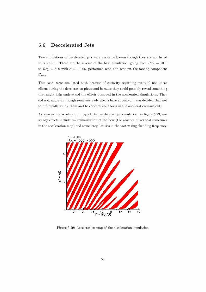
5.6 Deccelerated Jets

Two simulations of decelerated jets were performed, even though they are not listed

in table 5.1. These are the inverse of the base simulation, going from ReiD = 1000

to RefD = 500 with α = −0.06, performed with and without the forcing component

Uforc.

This cases were simulated both because of curiosity regarding eventual non-linear

effects during the deceleration phase and because they could possibly reveal something

that might help understand the effects observed in the accelerated simulations. They

did not, and even though some unsteady effects have appeared it was decided then not

to profoundly study them and to concentrate efforts in the acceleration issue only.

As seen in the acceleration map of the decelerated jet simulation, in figure 5.29, un-

steady effects include re-laminarization of the flow (the absence of vortical structures

in the acceleration map) and some irregularities in the vortex ring shedding frequency.

Figure 5.29: Acceleration map of the deceleration simulation

58

Chapter 6

Conclusion

Three main subjects were investigated throughout this work on the near field of linearly

accelerated turbulent round jets. The first two subjects, kinematics of vortex motion

and topology of vortex rings during acceleration were studied here for the first time

as these were the first DNS and LES of accelerating round jets. The third and last

subject, entrainment, was studied with different techniques than those used in previous

experimental and numerical works.

6.1 Kinematics of Vortex Motion and Topology of

the Vortex Rings

6.1.1 Shear layer mode

Acceleration has a deep impact in the kinematics and topology on the jet’s near field

of coherent structures. Regardless of the Reynolds number, or of the acceleration rate

applied, as soon as acceleration starts the shear layer mode changes radically from

shedding big, low frequency vortex rings to smaller, higher frequency ones.

The small vortex rings shed during the acceleration phase go through primary and

secondary merging events. The primary events happen close to the inlet for high

acceleration rates, but can happen as far as x/D = 7 for slow acceleration rates.

The size of the vortex rings and their merging events are closely related to the shear

59

a) b)

Figure 6.1: Sketch of the flow during the a) stationary phase, and b) accelerating phase

layer change during acceleration. As the jet starts to accelerate, the shear layer fre-

quency rises to much higher values than before, even though the acceleration is linear.

For this to happen the local topology of the flow (size of the primary vortex rings) has

necessarily changed.

From the Helmoltz theory for an isolated ring, the circulation Γring of the ring is given

by:

Γring ∼ UinjD (6.1)

and its vorticity, Ωring by:

Ωring ∼ Γringa

(6.2)

where Uinj is the injection velocity which gives birth to the ring and a is the vortex

core radius.

Furthermore, the convection velocity of the rings is given by:

Uv ∼ ΓringR

(6.3)

where R is the ring radius.

Hence, for the stationary jet case, the total vorticity of a box of unitary lenght (as

sketched in figure 6.1 a).) is:

Ωbox ∼ ΩringfUv

(6.4)

When the jet is linearly accelerating, Uinj is linearly increasing, so, both the vorticity

of each ring and its convection velocity are also linearly increasing:

Ωaring ∼ αt (6.5)

Uav ∼ βt (6.6)

60

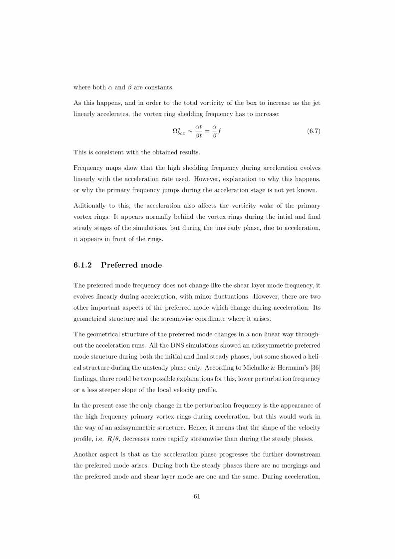
where both α and β are constants.

As this happens, and in order to the total vorticity of the box to increase as the jet

linearly accelerates, the vortex ring shedding frequency has to increase:

Ωabox ∼αt

βt=α

βf (6.7)

This is consistent with the obtained results.

Frequency maps show that the high shedding frequency during acceleration evolves

linearly with the acceleration rate used. However, explanation to why this happens,

or why the primary frequency jumps during the acceleration stage is not yet known.

Aditionally to this, the acceleration also affects the vorticity wake of the primary

vortex rings. It appears normally behind the vortex rings during the intial and final

steady stages of the simulations, but during the unsteady phase, due to acceleration,

it appears in front of the rings.

6.1.2 Preferred mode

The preferred mode frequency does not change like the shear layer mode frequency, it

evolves linearly during acceleration, with minor fluctuations. However, there are two

other important aspects of the preferred mode which change during acceleration: Its

geometrical structure and the streamwise coordinate where it arises.

The geometrical structure of the preferred mode changes in a non linear way through-

out the acceleration runs. All the DNS simulations showed an axissymmetric preferred

mode structure during both the initial and final steady phases, but some showed a heli-

cal structure during the unsteady phase only. According to Michalke & Hermann’s [36]

findings, there could be two possible explanations for this, lower perturbation frequency

or a less steeper slope of the local velocity profile.

In the present case the only change in the perturbation frequency is the appearance of

the high frequency primary vortex rings during acceleration, but this would work in

the way of an axissymmetric structure. Hence, it means that the shape of the velocity

profile, i.e. R/θ, decreases more rapidly streamwise than during the steady phases.

Another aspect is that as the acceleration phase progresses the further downstream

the preferred mode arises. During both the steady phases there are no mergings and

the preferred mode and shear layer mode are one and the same. During acceleration,

61

as smaller, high frequency rings are shed and differences arise between the two primary

instability modes, mergings of primary rings start to happen. These mergings happen

at first very close to the inlet but by the end of the acceleration phase happen much

further downstream, even after the end of the potential core. They stop in the instant

that acceleration ends.

6.1.3 Secondary instabilities

Given the limited streamwise length of the computational box it was not possible to

observe these instabilities at all the stages of the different simulations, limiting the

ability to conclude about the differences in their structure during the diverse phases.

Still, it was observed in the direct numerical simulations that they were visible only

during the last steady phase, meaning that the acceleration slows the transition pro-

cess. This is consistent with the previously discussed fact that the preferred mode

arises later downstream during the acceleration phase.

6.2 Entrainment Rate

As already discussed, all the previous works on accelerated round jets pointed to a

reduction in the entrainment rate of the jet during acceleration. This was usually

based on jet width measurements, passive scalar concentration pictures or, in the

case of Roy & Johari’s computational work [42], an inlet-normalized measure of the

streamwise evolution of the jet’s mass flow rate.

Conclusions on the jet’s entrainment rate should not be taken from jet width mea-

surements due to the pressure decrease in the jet core as the inlet, and hence, the

centerline, velocities increase. As seen in the present work, it is possible to have a

thinner jet which entrains more.

Passive scalar concentration measurements should, in principle, give a much more ac-

curate picture of the entrainment rate. In fact, carefully analyzing the pictures from

the Zhang & Johari experiment [50] on table 6.2 (which have already been shown in

section 3.2) it can be seen that the in the last instants of the acceleration (in the

picture on the right) not only the jet seems to be thinner, but also the dye concen-

tration is smaller than in the first picture, prior to the acceleration, meaning that the

62

entrainment rate might be higher during the unsteady phase. This was not noted in

their description of the results.

Figure 6.2: Dye concentration on experiment by Zhang & Johari [50]

Furthermore, the computational work by Roy & Johari was, a priori, dependent on

existing turbulence models probably not suited to cope with the unsteady effects now

found regarding the kinematics of the unsteady jet’s near field. Added to this, the way

that the entrainment rate was evaluated, via the normalized mass flow rate profiles,

might have led to a different conclusion on this matter.

In this work, based on radial velocity profiles and entrainment profiles calculated from

them, it is concluded that the unsteady turbulent jet under linear acceleration can

indeed have higher entrainment rates than when in a steady state.

63

Appendix A

Q Criteria Visualization

In order not to overfill chapter 5 with post-processing figures, this appendix presents

3D iso-surfaces and 2D contours of positive Q and the most relevant acceleration maps.

In the digital version of this thesis there are also movies available, covering most of

the discussed quantities in this thesis.

64

Q iso-surface

ReiD = 500

ReiD = 1000

ReiD = 10000

Table A.1: 3D iso-surfaces of Q

65

ReiD

ReiD = 500

ReiD = 1000

ReiD = 10000

Table A.2: 2D contours of positive Q during the initial phase

66

Accelerating

ReiD = 500

ReiD = 1000

ReiD = 10000

Table A.3: 2D contours of positive Q during acceleration

67

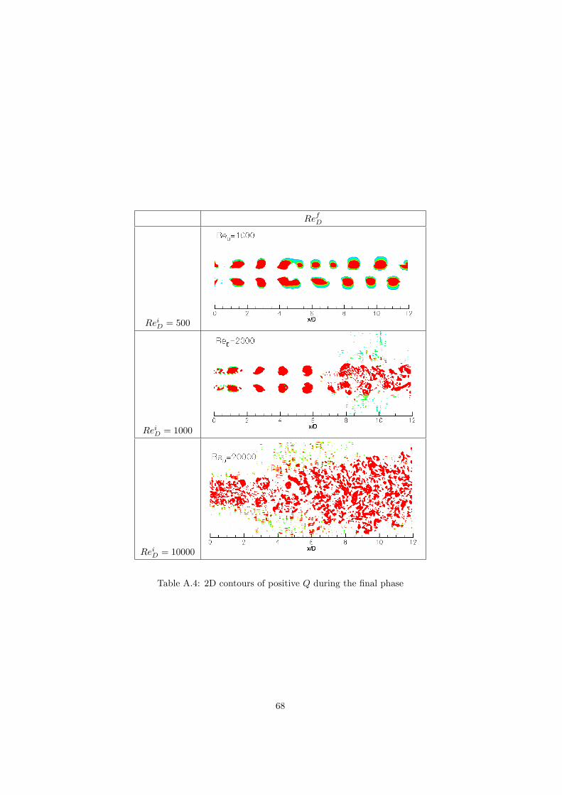
RefD

ReiD = 500

ReiD = 1000

ReiD = 10000

Table A.4: 2D contours of positive Q during the final phase

68

ReiD = 500

Table A.5: Acceleration maps

69

ReiD = 500

Table A.6: Acceleration maps

70

α = 0.06

Table A.7: Acceleration maps

71

Appendix B

Article no. 1

72

The effects of acceleration in jets: kinematics of the near field vortices

Carlos B. da Silva, Pedro Neto and Jose C.F. PereiraIDMEC/IST Technical University of Lisbon,

Mecanica I, 1o andar (LASEF),Av. Rovisco Pais, 1049-001 Lisboa, Portugal

(Dated: September 10, 2008)

Direct and large-eddy simulations (DNS/LES) of accelerating round jets are used to analyze theeffects of acceleration on the kinematics of the coherent structures from the near field of roundjets (x/D < 12). The acceleration is obtained by increasing the nozzle jet velocity with time, ina previously established (steady) jet. Several acceleration rates (α = 0.02 − 0.6) and Reynoldsnumbers (ReD = 500 − 1000, 1000 − 2000, and 10000 − 20000) were simulated. The accelerationdecreases the spreading rate of the jet, in agreement with previous experimental works. Detailedacceleration maps are used to track down the kinematics of the vortex motion in the near field ofthe jet and show that during the acceleration phase the near field coherent vortices (rings) becomesmaller and are formed at an higher frequency than in the steady jet. This shedding frequencyincreases (linearly) with the acceleration rate which causes a number of new primary and secondaryvortex merging events in the near field of the jet that are absent from steady jets.

PACS numbers: 47.15.St, 47.27.De, 47.27.ek, 47.27.ep, 47.27.wg, 47.32.C-

Introduction Jet control has been studied extensivelydue to its numerous potential industrial applications e.g.mixing, combustion, and aero-acoustics. However, a rel-atively small number of works analyzed the effects of ac-celeration in jets, where the acceleration consists in in-creasing the nozzle jet velocity - and thus the mass flowrate and the Reynolds number - in a previously estab-lished (steady) jet.

Breidenthal [1] postulated the existence of a new self-similar turbulent jet - the exponential jet - where eacheddy has constant vorticity throughout its life. For this tooccur the nozzle exit speed must increase exponentiallywith time. He inferred that the entrainment of ambi-ent fluid is strongly inhibited in these jets because the”entrainment appetite” of the coherent structures fromthe jet is completely satisfied by the accelerating noz-zle stream. Measurements of linearly accelerating jets(starting with zero nozzle velocity) were made by Katoet al. [2] and showed that the acceleration modifies sig-nificantly both the jet mixing and the entrainment ratecompared to the steady jet. Kouros et al. [3] reportedthe spreading rate and penetration length in experimen-tal accelerated jets generated from gravity an found thatthe spreading rate of the accelerated jet was about 50%smaller than the classical (steady) jet.

Zhang and Johari [4] studied experimentally the effectsof acceleration in jets using linear, quadratic and expo-nential accelerations, where the acceleration starts in apreviously established (steady) jet with Reynolds num-ber ReD = 3 × 103 and ends once the Reynolds numberreaches ReD = 3 × 104. For each type of accelerated jetseveral acceleration rates were considered. As the flowaccelerated a discernible ”front” was established whereparcels of less diluted dye are seen to travel downstreamat a given (constant) speed. This speed was observed todepend on the acceleration rate and a model for the evo-lution of the front position was developed. They observed

also, in agreement with previous works, that the acceler-ation decreases the visible spreading rate of acceleratingjets compared to a steady jet at the same Reynolds num-ber.

Johari and Paduano [5] studied the mixing in exper-imental gravity-driven jets where jet nozzle velocity in-creases initially from zero to a maximum, and decreasescontinually after. This study showed that in the sameway as the jet mixing and spreading rate is seen to in-crease during the acceleration phase, the inverse occursduring deceleration i.e. decelerated jets exhibit largerspreading and mixing rates compared to steady jets.

Recently Abani and Reitz [6] developed a model topredict the velocity distribution in round jets with timevarying nozzle velocities. The model is derived from theclassical Helmholtz vortex motion theory and was usedfor several shapes of the temporal nozzle jet velocity, in-cluding accelerated jets with linear, quadratic, and ex-ponential functions. They performed the first numer-ical study of unsteady accelerated jets using unsteadyReynolds averaged Navier-Stokes (URANS) simulationswith a variant of the k−ε turbulence model. Their modeland simulations showed good agreement with the exper-imental results of Zhang and Johari [4].

Since the jet dynamics, particularly in the near field,is to a large extent dictated by the large scale coherentvortices from the flow, it is important to understand thedynamics of these vortices in accelerated jets in order toexplain the observed effects of acceleration in the spread-ing and mixing rates of jets. As a first step towards thisgoal the present work uses direct and large-eddy simula-tions (DNS/LES) of accelerated jets in order to analyzethe kinematics of the near field coherent structures inthese flows. To the author’s knowledge this work presentsthe first DNS and LES of accelerated jets.

Numerical method The simulations were performedwith an highly accurate Navier-Stokes solver in which the

2

spatial derivatives are discretized using a 6th order Com-pact scheme in the streamwise (x) direction and pseudo-spectral methods in the y and z directions. Temporal ad-vancement is achieved with an explicit, 3 step, 3rd order,low storage Runge-Kutta time stepping scheme[7].Thiscode was extensively validated in numerical simulationsof round, plane and coaxial jets (da Silva and Metais[7, 8], da Silva et al. [9]).

Physical and computational parameters The simula-tions reported here are very similar to the ”natural”jet simulations (”NLR” and ”NHR”) described in de-tail in da Silva and Metais [7]. Therefore only a briefdescription will be given here. As in reference [7] allthe simulations were carried out on the same mesh with201 × 128 × 128 grid points along the x, y, and zdirections, and the computational domain extends to12.25D×7D×7D along the streamwise and the two trans-verse directions, respectively, where D is the jet nozzlediameter. The ratio of the jet radius to the initial shearlayer momentum thickness is R/θ0 = 12. For each timestep t, a given velocity profile is prescribed at the in-let, ~U(~x0, t) = ~Umed(~x0, t) + ~Unoise(~x0, t) + ~Uforc(~x0, t),where ~U( ~x0, t) is the instantaneous inlet velocity vector,~Umed( ~x0, t) = (Umed, 0, 0) is the mean streamwise veloc-ity, and ~Unoise(~x0, t) is a function that sets a small ampli-tude spectral noise (1%) near the region with the highestmean velocity gradient (see da Silva and Metais [7]). Insome simulations a function ~Uforc(~x0, t) is used to im-pose a sinusoidal perturbation with prescribed frequencyf and 5% amplitude at the inlet nozzle of the jet. Theprescribed frequency was chosen to have a Strouhal num-ber equal to the preferred mode of the jet, which in thesesimulations is StD = 0.375. As in da Silva and Metais[7] Umed is given by a hyperbolic-tangent profile,

U1(t) + U2

2− U1(t)− U2

2tanh

[14

R

θ0

(r

R− R

r

)](1)

where U1(t) is the jet centerline velocity, U2 is a small co-flow and θ0 is the momentum thickness of the initial shearlayer. The acceleration is imposed through a functionthat sets a (linear) temporal variation on U1(t) definedin equation (1): U1(t) = U01 (1 + αt), where α is the ac-celeration parameter and U01 is the initial maximum jetvelocity. For each run, prior to the acceleration phase, allthe simulations were run for t∗0 = t(U01/D) = 40 in orderto allow the steady jet to be completely established. Theinitial Reynolds number of the flow is Rei

D = U01D/νand for t∗ ≥ t∗0 the acceleration phase starts. Duringthe acceleration the Reynolds number increases linearlywith time Rea

D(t) = U1(t)D/ν. The acceleration phaseends when the Reynolds number - and the jet centerlinevelocity U1(t) - reaches twice its initial value i.e. whenRef

D = 2ReiD. Notice that the ratio R/θ = 12 is main-

tained throughout the acceleration.Several DNS and LES of accelerating jets were car-

ried out using various acceleration rates α. The mainbulk of the simulations consists in DNS where the final

TABLE I: Non-dimensional time elapsed during the acceler-ation phase for each acceleration parameter.

α 0.02 0.04 0.06 0.08 0.10 0.20 0.40 0.60

∆t∗ 40-90 40-65 40-57 40-53 40-50 40-45 40-43 40-41

x/D

δ(x)

/D

0 2 4 6 8 10 120.6

0.8

1

1.2

1.4t*=32t*=48t*=63t*=76t*=88

α=0.02

x/D

δ(x)

/D

0 2 4 6 8 10 120.6

0.7

0.8

0.9

1

1.1

1.2

1.3

α=0.02α=0.04α=0.06α=0.08

t*=48

(a) (b)

FIG. 1: Instantaneous shear layer thickness δ(x) for acceler-ated jets: (a) as function of time for the simulation with ac-celeration rate α = 0.02; (b) at non-dimensional time t∗ = 48for several acceleration rates α = 0.02, 0.04, 0.06, and 0.08.

Reynolds number (after the acceleration) is RefD = 1000

(ReiD = 500). Table I lists the values of α used and

the non-dimensional time elapsed during the accelera-tion phase for each case. Another set of DNS was runfor Ref

D = 2000, and LES using the Filtered structurefunction model (Ducros et al. [10]) were also performedwith Ref

D = 20000. In most simulations the imposed si-nusoidal perturbation ~Uforc(~x0, t) was used in order toallow an easier tracking of the flow coherent structuresduring the acceleration phase, however several simula-tions were also carried out without this forcing functionin order to assess if its presence influences the results ob-tained. As described below the forcing frequency doesnot influence the main results and conclusions.

Effect of acceleration in the spreading rate of jets Inagreement with all the previous experimental works onaccelerated jets e.g. Zhang and Johari [4] in all our sim-ulations we observed that during the acceleration phasethe spreading rate of the jet decreases compared to thespreading rate of the steady jet. To illustrate this Fig. 1(a) shows the instantaneous jet half-width δ(x) obtainedwith the instantaneous velocity field of the jet for thesimulation with α = 0.02. Prior the acceleration phasethe instantaneous half-width shows some wiggles whichare caused by the passage vortex ring structures. Afterthe start of the acceleration (t∗ = 40) the jet half-widthdecreases with time attaining a more or less constantfunction during rest of the acceleration. After the accel-eration phase the jet half-width rises again. Moreover,in agreement with Zhang and Johari [4], the decrease ofthe jet spreading rate is higher for higher accelerationrates as shown in Fig. 1 (b) where instantaneous valuesof δ(x) are shown at a given time from the start of theacceleration phase t∗ = 48 for several acceleration rates.

3

FIG. 2: Iso-surfaces of positive Q, where Q is the secondinvariant of the velocity gradient tensor in the near field(x/D < 12) of the accelerating jet simulation with α = 0.06.

Coherent vortices in the near field of accelerating jetsFigure 2 shows iso-surfaces of positive Q where Q =12 (ΩijΩij − SijSij) is the second invariant of the velocitygradient tensor for simulation with α = 0.06. Prior tothe acceleration, in agreement with da Silva and Metais[7], at the end of the potential core the flow exhibitsring shaped vortices that are shed with a frequency cor-responding to a Strouhal number of StrD = fD/U1 =0.375, indicating the jet preferred mode. However, duringthe acceleration the flow forms vortex rings with smallercore diameter than in the steady jet (aa < ai), and theseare shed at an higher frequency than the preferred mode.Figure 2 corresponds to t∗ = 45 i.e. shortly after thestart of the acceleration, and still shows the larger ringvortices from the steady jet regime, which are followed bysmaller ring shaped vortices generated during the accel-eration phase. Due to the acceleration some vortex ringsmerge generating new (larger) vortices. After the accel-eration phase the flow again exhibits vortex ring struc-tures that are shed at a frequency corresponding to thejet preferred mode.

Acceleration maps In order to analyze the kinematicsof the vortex ring motion we use acceleration maps wherefor each time we plot the instantaneous value of Q(x, r, t),where r is the radial coordinate where the mean velocityis half its maximum. The vortex rings are identified bythe threshold Q ≥ 0.01(U01/H). Plotting all the linesof Q(x, r, t) for each time t we obtain the accelerationmaps. Figure 3 shows the acceleration map for α = 0.06between 30 < t∗ < 70 and illustrates the typical featuresof accelerated jets. The trajectory of each vortex ring isclearly identified in these figures by the grey oblique lines.The local velocity of each ring is equal to the slope of thetangent to its trajectory line v∗ = ∂x∗/∂t∗, and the fre-quency of the vortex ring shedding may be obtained fromthe distance between two neighboring trajectory lines fora given axial distance x∗. One observes clearly three dis-tinct zones before (t∗ < 40), during (40 < t∗ < 57), andafter (t∗ > 57) the acceleration. Outside the accelera-

FIG. 3: Acceleration map for the simulation with α = 0.06showing the trajectories of the vortex rings before (t∗ < 40),during (40 < t∗ < 57), and after (t∗ > 57) the accelerationphase.

tion phase the vortex rings travel with an approximatelyconstant speed, where v∗(t∗ > 57) > v∗(t∗ < 40) dueto the higher mean jet velocity after the acceleration.Notice that during the acceleration phase the sheddingfrequency of the vortex rings is higher than before or af-ter the acceleration. Merging events between vortex ringsare identified when two vortex trajectories merge into onee.g. a primary merging event occurs at (t∗, x∗) ≈ (50, 4),and a secondary merging occurs at (t∗, x∗) ≈ (58, 10). Aseries of primary merging events takes place at a meandistance of about HA = x∗ ≈ 4, while secondary mergeroccurs at about HB = x∗ ≈ 8 − 10. Using the acceler-ation maps we computed the mean location for the pri-mary merging events HA for all the acceleration rates α.The results are displayed in Fig. 4 (a) and show that HA

decreases as the acceleration rate increases from HA = 7for α = 0.02 to HA = 0 for α = 0.04 and 0.06 i.e. forthe largest acceleration rates used in this study no pri-mary merger can be observed for the initial vortex ringstructures, since the acceleration phase is too short.

Number of merging events in accelerating jets The ac-celeration maps were used to compute the number of pri-mary and secondary merging events between vortex ringsfor all the simulations. The results are displayed in Fig.4 (b) and show that, provided there is time enough forthe initial vortex rings to merge (α ≤ 0.2), the numberof these events is relatively independent from the valueof α and alternates between 8 and 5 for all but one of theacceleration rates considered in this study. This can beexplained by the fact that the acceleration rate increasesthe frequency of the vortex rings formed during the accel-eration phase. Finally note that the number of secondarymerging events also stays more or less constant.

Vortex shedding frequency in accelerating jets Figure5 (a) shows the vortex shedding frequency of the pri-mary rings at x∗ = x/D = 2 computed from the accel-eration maps for several acceleration rates. Before andafter the acceleration phase the rings are advected witha frequency that is exactly equal to the prescribed fre-quency - chosen as the preferred jet mode. However, for

4

α

<HA>

0 0.1 0.2 0.3 0.4 0.5 0.60

2

4

6

8

10

α0 0.1 0.2 0.3 0.4 0.5 0.60

2

4

6

8

10 PrimarySecondaryTotal

Merging events

(a) (b)

FIG. 4: Statistics for vortex ring merging in accelerating jetsfor several acceleration rates α: (a) average location of theprimary merging event HA; (b) number of primary and sec-ondary merging events.

t*

freq

.

40 50 60 700

0.5

1

1.5

2

2.5

3

3.5

pre α=0.04pre α=0.06pre α=0.04sim α=0.08sim α=0.06sim α=0.08

x/D=2

α

<fA>

0 0.02 0.04 0.06 0.08 0.11

1.5

2

2.5

3

(a) (b)

FIG. 5: Vortex ring shedding frequency during acceleration atx/D = 2 i.e. before the primary merging events: (a) duringthe simulation (’pre’ - prescribed at the inlet, ’sim’ - from thesimulation); (b) mean value during the acceleration.

some reason during the acceleration phase the rings areformed at higher frequency than the imposed (forced)frequency, and this frequency increases during the accel-eration phase. Once the acceleration ends the flow needssome time to recover the preferred jet mode, and thisrecovery time also increases with the acceleration rate α.

Figure 5 (b) shows that the mean vortex shedding fre-quency < fA > as function of α is approximately linearduring the acceleration. The mechanisms behind thissurprising behavior of the vortex shedding frequency areunclear at the moment, however this result is consistentwith the inviscid theory of isolated vortex rings: since the

circulation of the rings Γ increases linearly with time forlinearly accelerated jets[6] the same has to be true also ofthe vorticity of individual rings Ω ∼ Γ/a2 (a is the coreradius of the rings). Consider a given region of spacee.g. a box domain (of unit length) enclosing rings in thenear field of the jet. The total vorticity in this box for asteady jet is Ωbox ∼ Ωf/UT where f is the vortex shed-ding frequency and UT ∼ Γ/R is the speed of the vortexrings of radius R. The frequency f has to increase withtime for the total box vorticity to increase also duringthe acceleration. A somehow similar phenomena seemsto occur in vortex rings generated from piston/cylinderarrangement with large piston stroke to diameter ratios(Gharib et al. [11]).

Influence of the Reynolds number and forcing frequencyIn order to assess if the Reynolds number or the pre-scribed forcing frequency modify the results describedabove several new simulations were carried out: a DNSwith Ref

D = 2000 and an LES with RefD = 20000, both

for α = 0.06. Moreover, all the simulations were runagain, including the new DNS and LES, but withoutadding any forcing frequency to the inlet instantaneousvelocity profile. It is more difficult to analyze the kine-matics of the coherent vortices with these new simula-tions using the acceleration maps alone since the nearfield vortex rings are much more fragmented and are moredifficult to track down, however visualizations, anima-tions, and energy spectra at several different locationsshowed that the Reynolds number and forcing frequencyhave no effect on the previous results.

Conclusion This work presents the first DNS andLES of accelerated jets, where the acceleration is ob-tained by increasing the mass flow rate in a previouslyestablished (steady) jet. In agreement with previous ex-perimental works the acceleration decreases the spread-ing rate of the jet during acceleration. The main effectof the acceleration on the kinematics of the near fieldprimary vortex ring structures is to increase their shed-ding frequency compared to the preferred frequency ofthe steady jet. This results in a number of primary andsecondary vortex merger events in the near field of the ac-celerating jet. The number of these merger events seemsto be relatively independent of the acceleration rate α forthe range of accelerations studied in this work.

[1] R. R. Breidenthal, Phys. Fluids 29, 2346 (1986).[2] S. Kato, B. Groenewegen, and R. Breidenthal, AIAA

Journal 25, 165 (1986).[3] H. Kouros, R. Medina, and H. Johari, AIAA Journal 31,

1524 (1993).[4] Z. Zhang and H. Johari, Phys. Fluids 8, 2185 (1996).[5] H. Johari and R. Paduano, Expts. Fluids 23, 272 (1997).[6] N. Abani and R. Reitz, Phys. Fluids 19, 125102 (2007).[7] C. B. da Silva and O. Metais, Phys. Fluids 14(11), 3798

(2002).

[8] C. B. da Silva and O. Metais, J. Fluid Mech. 473, 103(2002).

[9] C. B. da Silva G. Balarac and O. Metais, Journal of Tur-bulence 024(4) (2003).

[10] F. Ducros, P. Comte, and M. Lesieur, J. Fluid Mech.326, 1 (1996).

[11] M. Gharib, E. Rambod, and K. Shariff, J. Fluid Mech.360, 121 (1998).

Bibliography

[1] N. Abani and R. D. Reitz. Unsteady turbulent round jets and vortex motion.

Physics of Fluids, 19:125102, 2007.

[2] C. Bogey and C. Baily. Large eddy simulations of transitional round jets: Influence

of the reynolds number on flow development and energy dissipation. Physics of

Fluids, 18:065101, 2006.

[3] P. Brancher, J. M. Chomax, and P. Huerre. Direct numerical simulations of round

jets: Vortex induction and side jets. Physics of Fluids, 6(5):1768–1774, 1994.

[4] R. Breidenthal. The turbulent exponential jet. Physics of Fluids, 29:2346–2374,

1986.

[5] J. Cohen and I. Wygnaski. The evolution of instabilities in the axissymetric jet.

part 1: The linear growth of the disturbances near the nozzle. Journal of Fluid

Mechanics, 176:191–219, 1987.

[6] D. G. Crighton and M. Gaster. Stability of slowly divergent jet flow. Journal of

Fluid Mechanics, 76:397–413, 1979.

[7] S. C. Crow and F. H. Champagne. Oderly structure in jet turbulence. Journal of

Fluid Mechanics, 48:547–591, 1971.

[8] C. B. da Silva. The role of coherent structures in the control and interscale inter-

actions of round, plane and coaxial jets. PhD thesis, INPG, Grenoble, 2001.

[9] C. B. da Silva, C. Balarac, and O. Metais. Transition in high velocity ration

coaxial jets analysed by direct numerical simulations. Journal of Turbulence,

4:024, 2002.

77

[10] C. B. da Silva and O. Metais. On the influence of coherent structures upon inter-

scale interactions in turbulent plane jets. Journal of Fluid Mechanics, 473:103–

145, 2002.

[11] C. B. da Silva and O. Metais. Vortex control of bifurcating jets: a numerical

study. Physics of Fluids, 14:3798–3819, 2002.

[12] J. O. Dabiri and M. Gharib. Fluid entrainment by isolated vortex rings. Journal

of Fluid Mechanics, 511:311–331, 2004.

[13] I. Danaila, J. Dusek, and F. Anselmet. Coherent structures in a round, spatial

evolving, unforced, homogeneous jet at low reynolds numbers. Physics of Fluids,

9(11):3323–3342, 1997.

[14] V. de Brederode. Fundamentos de Aerodinamica Incompressıvel. 1997.

[15] T. Djeridane. Contribuition a l’etude experimentale de jets turbulents ax-

isymetriques a densite variable. PhD thesis, Universie d’Aix-Marseille II, 1994.

[16] F. Ducros, P. Comte, and M. Lesieur. Large-eddy simulation of transition to

turbulence in a boundary layer developing spatially over a flat plate. Journal of

Fluid Mechanics, 326:1–36, 1996.

[17] M. V. Dyke. An Album of Fluid Motion. 1982.

[18] P. Freimuth. On transition in a separated laminar boundary layer. Journal of

Fluid Mechanics, 25:683, 1966.

[19] U. Frisch. Turbulence - The Legacy of A. N. Kolmogorov. 1995.

[20] B. J. Geurts. Elements of direct and large-eddy simulation. 2004.

[21] M. A. Gonze. Simulation numerique des sillages en transition a la turbulence.

PhD thesis, INPG, Grenoble, 1993.

[22] F. F. Grinstein, M. Glauser, and W. K. George. Fluid Vortices, chapter 3, pages

65–94. Kluwer Academic Publishing, 1995.

[23] E. Gutmark and I. Wygnansky. An analysis of subgrid-scale interactions in nu-

merically simulated isotropic turbulence. Journal of Fluid Mechanics, 73:465–495,

1976.

78

[24] A. Hussein and K. Zaman. Vortex pairing in a circular jet under controlled

excitation. part 2: Coherent structures dynamics. Journal of Fluid Mechanics,

101:493–544, 1980.

[25] H. Johari and R. Paduano. Dillution and mixing in an unsteady jet. Experiments

in Fluids, 23:272–280, 1997.

[26] Kato, Groenewegen, and Breidenthal. Turbulent mixing in nonsteady jets. AIAA

Journal, 25:165–167, 1986.

[27] H. Kouros, R. Medina, and H. Johari. Turbulent mixing in nonsteady jets. AIAA

Journal, 29:1524–1526, 1993.

[28] S. J. Kwon and I. W. Seo. Reynolds number effects on the behavior of a non-

buoyant round jet. Experiments in Fluids, 38:801–812, 2005.

[29] S. K. Lele. Compact finite difference schemes with spectral-like resolution. Journal

of Computational Physics, 103:15 – 42, 1992.

[30] D. Liepmann and M. Gharib. The role of streamwise vorticity in the near field

entrainment of round jets. Journal of Fluid Mechanics, 245:643–668, 1992.

[31] T. T. Lim and T. B. Nickels. Fluid Vortices, chapter 4, pages 95–153. Kluwer

Academic Publishing, 1995.

[32] T. Maxworthy. The structure and stability of vortex rings. Journal of Fluid

Mechanics, 51:15–32, 1972.

[33] M. V. Melander, F. Hussain, and A. Basu. Breakdown of a circular jet into

turbulence. In Eight symposium on turbulent shear flows, pages 15.5.1–15.5.6,

1991.

[34] A. Michalke. On the inviscid instability of the hiperbolic-tangent velocity profile.

Journal of Fluid Mechanics, 19:543–556, 1964.

[35] A. Michalke. On spatially growing disturbances in an inviscid shear layer. Journal

of Fluid Mechanics, 23:521–544, 1965.

[36] A. Michalke and G. Hermann. On the inviscid instability of a circular jet with

external flow. Journal of Fluid Mechanics, 114:343–359, 1982.

[37] P. A. Monkewitz and P. Huerre. Influence of the velocity ration on the spatial

instability of mixing. Physics of Fluids, 25(7):1137–1143, 1982.

79

[38] H. Moravec. Robots, after all. In Comunications of the ACM. August 2003.

[39] M. Olsson and L. Fuchs. A simple boundary condition for unbounded hyperbolic

flows. Physics of Fluids, 8(8):2125–2137, 1996.

[40] I. Orlansky. A simple boundary condition for unbounded hyperbolic flows. Journal

of Computational Physics, 21:251–269, 1976.

[41] P. Plaschko. Helical instabilities of slowly divergent jets. Journal of Fluid Me-

chanics, 92:209–215, 1979.

[42] R. R. Roy and H. Johari. Finite element analysis of an accelerating turbulent

round jet. In Recent advances in mechanics of structured continua. 1993.

[43] P. G. Saffman. The number of waves on unstable vortex rings. Journal of Fluid

Mechanics, 84:625–639, 1978.

[44] S. Stanley and S. Sarkar. A study of the flowfield evolution and mixing in a planar

turbulent jet using direct numerical simulation. Journal of Fluid Mechanics, 1999.

[45] G. Urbin and O. Metais. Direct and Large-Eddie Simulations II, pages 539–542.

Kluwer Academic Publishing, 1997.

[46] R. Verzico and P. Orlandi. Direct simulations of the transitional regime of a

circular jet. Physics of Fluids, 6(2):751–759, 1994.

[47] S. E. Widnall, D. B. Bliss, and C.-Y. Tsai. Instability of short waves on a vortex

ring. Journal of Fluid Mechanics, 66:35–47, 1974.

[48] J. H. Williamson. Low-storage runge-kutta schemes. Journal of Computational

Physics, 35:48–56, 1980.

[49] K. Zaman and A. Hussein. Vortex pairing in a circular jet under controlled

excitation. part 1: General jet response. Journal of Fluid Mechanics, 101:449–

491, 1980.

[50] Z. Zhang and H. Johari. Effects of acceleration on turbulent jets. Physics of

Fluids, 8:2185–2195, 1996.

80