Numerical Simulation Of Three-Dimensional Free Surface Film Flow Over Or Around Obstacles On An...
236
-
Upload
kian-chuan -
Category
Documents
-
view
16 -
download
1
description
Within the bearing chamber of a gas turbine aero-engine, lubrication of the shaft andother bearings is achieved by an oil lm which may become signicantly disturbed byinteracting with a range of chamber geometries which protrude from the chamber wall.Minimizing these disturbances and preventing possible dry areas is crucial in optimizinga bearing chambers design. In addition, multiple obstructions may be located closeto one another, resulting in a more complex disturbed lm prole than by individualobstacles. Prediction of the disturbance of the lm is an important aspect of bearingchamber design.
Transcript of Numerical Simulation Of Three-Dimensional Free Surface Film Flow Over Or Around Obstacles On An...

Numerical Simulation Of
Three-Dimensional Free Surface Film Flow
Over Or Around Obstacles
On An Inclined Plane
Steven J. Baxter, MMath (Hons).
Thesis submitted to the University of Nottingham
for the degree of Doctor of Philosophy
July 2010
Abstract
Within the bearing chamber of a gas turbine aero-engine, lubrication of the shaft and
other bearings is achieved by an oil lm which may become signicantly disturbed by
interacting with a range of chamber geometries which protrude from the chamber wall.
Minimizing these disturbances and preventing possible dry areas is crucial in optimizing
a bearing chambers design. In addition, multiple obstructions may be located close
to one another, resulting in a more complex disturbed lm prole than by individual
obstacles. Prediction of the disturbance of the lm is an important aspect of bearing
chamber design.
For analysis of the lm prole over or around a local obstacle, typical bearing chamber
ows can be approximated as an incompressible thin lm ow down an inclined wall
driven by gravity. The Reynolds number of thin lm ows is often small, and for the bulk
of this thesis a Stokes ow assumption is implemented. In addition, thin lms are often
dominated by surface tension eects, which for accurate modelling require an accurate
representation of the free surface prole. Numerical techniques such as the volume of
uid method fail to track the surface prole specically, and inaccuracies will occur in
applying surface tension in this approach. A numerical scheme based on the boundary
element method tracks the free surface explicitly, alleviating this potential error source
and is applied throughout this thesis. The evaluation of free surface quantities, such
as unit normal and curvature is achieved by using a Hermitian radial basis function
interpolation. This hermite interpolation can also be used to incorporate the far eld
ii

boundary conditions and to enable contact line conditions to be satised for cases where
the obstacle penetrates the free surface.
Initial results consider a lm owing over an arbitrary hemispherical obstacle, fully
submerged by the uid for a range of ow congurations. Comparison is made with
previously published papers that assume the obstacle is small and / or the free surface
deection and disturbance velocity is small. Free surface proles for thin lm ows over
hemispherical obstacles that approach the lm surface are also produced, and the eects
of near point singularities considered. All free surface proles indicate an upstream peak,
followed by a trough downstream of the obstacle with the peak decaying in a horseshoe
shaped surface deformation. Flow proles are governed by the plane inclination, the
Bond number and the obstacle geometry; eects of these key physical parameters on
ow solutions are provided.
The disturbed lm proles over multiple obstacles will dier from the use of a single
obstacle analysis as their proximity decreases. An understanding of the local interaction
of individual obstacles is an important aspect of bearing chamber design. In this thesis
the single obstacle analysis is extended to the case of ow over multiple hemispheres.
For obstacles that are separated by a suciently large distance the ow proles are
identical to those for a single obstacle. However, for ow over multiple obstacles with
small separation, variations from single obstacle solutions maybe signicant. For ow
over two obstacles placed in-line with the incident ow, variations with ow parameters
are provided. To identify the exibility of this approach, ows over three obstacles are
modelled.
The calculation of ows around obstacles provides a greater challenge. Notably, a static
contact line must be included such that the angle between the free surface and the
obstacle is introduced as an extra ow parameter that will depend both on the uid and
the obstacle surface characteristics. The numerical models used for ow over hemispheres
can be developed to consider lm ow around circular cylinders. Numerical simulations
iii
are used to investigate ow parameters and boundary conditions. Solutions are obtained
where steady ow proles can be found both over and around a cylindrical obstacle
raising the awareness of possible multiple solutions.
Flow around multiple obstacles is also analyzed, with proles produced for ow around
two cylinders placed in various locations relative to one another. As for ow over two
hemispheres, for suciently large separations the ow proles are identical to a single
obstacle analysis. For ow around two obstacles spaced in the direction of the ow,
eects of altering the four governing parameters; plane inclination angle, Bond number,
obstacle size, and static contact angle are examined. The analysis of ow around three
cylinders in two congurations is nally considered. In addition, for two obstacles spaced
in-line with the incident ow, the numerical approaches for ow over and ow around are
combined to predict situations where ow passes over an upstream cylinder, and then
around an identical downstream cylinder.
The nal section of this thesis removes the basic assumption of Stokes ow, through
solving the full Navier-Stokes equations at low Reynolds number and so incorporating
the need to solve nonlinear equations through the solution domain. An ecient nu-
merical algorithm for including the inertia eects is developed and compared to more
conventional methods, such as the dual reciprocity method and particular integral tech-
niques for the case of a three-dimensional lid driven cavity. This approach is extended
to enable calculation of low Reynolds number lm proles for both ow over and around
a cylinder. Results are compared to the analysis from previous Stokes ow solutions for
modest increases in the Reynolds number.
iv

List Of Publications
S. J. Baxter, H. Power, K. A. Clie and S. Hibberd. Simulation of thin lm ow around a
cylinder on an inclined plane using the boundary element method. In Boundary Elements
and Other Mesh Reduction Methods XXX. Maribor, Slovenia (WIT Press, 2008) ISBN:
978-1-84564-121-4
S. J. Baxter, H. Power, K. A. Clie and S. Hibberd. Three-Dimensional Thin Film Flow
Over and Around an Obstacle on an Inclined Plane. Physics of Fluids. (3) 21 (2009)
S. J. Baxter, H. Power, K. A. Clie and S. Hibberd. Free surface Stokes ows obstructed
by multiple obstacles. Published Online; International Journal for Numerical Methods
in Fluids DOI:10.1002/d.2029. (2009)
S. J. Baxter, H. Power, K. A. Clie and S. Hibberd. Numerical Simulation Of A Free
Surface Stokes Flow Around Multiple Cylinders On An Inclined Plane Using A Boundary
Element Method And Radial Basis Function Approach. In Grand Review in the State-of-
the-Art in the Numerical Simulation of Fluid Flow London, United Kingdom (IMechE,
2009)
S. J. Baxter, H. Power, K. A. Clie and S. Hibberd. An Ecient Numerical Scheme For
A Low Reynolds Number Flow In A Three-Dimensional Lid-Driven Cavity. In Seventh
UK conference on Boundary Integral Methods. Nottingham, United Kingdom (University
of Nottingham, 2009) ISBN: 978-0-9563221-0-4
v

Award for best poster by a PhD student: Numerical Simulation of Thin Films
Over and Around Obstacles. 50th British Applied Mathematics Colloquium (University
of Manchester, 2008).
vi

Acknowledgements
I gratefully acknowledge my supervisors, Henry Power, Andrew Clie and Stephen Hib-
berd, for their guidance and hard work throughout this project. Without their support,
this PhD would not have been possible.
I would also like to thank the EPSRC and Rolls-Royce, for the nancial support they
have provided throughout this project.
The PhD was carried out at the University Technology Centre in Gas Turbine Trans-
mission Systems at the University of Nottingham, and I am grateful to all my friends
and colleagues for contributing to my time at the University.
I wish to thank my parents and the rest of my family for their continuous encouragement
and support. Finally, to Charlotte, thank you for your unwavering love and patience,
and for keeping me sane.
vii
Contents
1 Introduction 1
1.1 Literature Overview . . . . . . . . . . . . . . . . . . . . . . . . . . . . . . 5
1.1.1 Physical Observation Of Film Flows . . . . . . . . . . . . . . . . . 5
1.1.2 Numerical Simulation Of Film Flows . . . . . . . . . . . . . . . . . 7
1.2 Thesis Structure . . . . . . . . . . . . . . . . . . . . . . . . . . . . . . . . 13
2 Viscous Flows 17
2.1 Introduction To Viscous Flows . . . . . . . . . . . . . . . . . . . . . . . . 17
2.2 An Overview Of The Boundary Integral Formulation . . . . . . . . . . . . 20
2.3 Direct Boundary Integral Equations For Stokes Flow . . . . . . . . . . . . 22
2.3.1 Derivation Of The Lorentz Reciprocal Relation . . . . . . . . . . . 23
2.3.2 Fundamental Solutions And Their Properties . . . . . . . . . . . . 24
2.3.3 Derivation Of The Direct Boundary Integral Equations . . . . . . . 30
viii

Contents
2.4 The Boundary Element Method . . . . . . . . . . . . . . . . . . . . . . . . 36
2.4.1 Approximation And Collocation . . . . . . . . . . . . . . . . . . . 37
2.4.2 Implementation Of A Constant Boundary Distribution . . . . . . . 39
3 Radial Basis Functions 42
3.1 Introduction To Radial Basis Function Interpolations . . . . . . . . . . . . 42
3.2 Local And Global Interpolations . . . . . . . . . . . . . . . . . . . . . . . 46
4 Stokes Flow Over A Single Obstacle 49
4.1 Mathematical Formulation . . . . . . . . . . . . . . . . . . . . . . . . . . . 49
4.1.1 Small Free Surface Deections . . . . . . . . . . . . . . . . . . . . . 57
4.1.2 Flow Over Asymptotically Small Obstacles . . . . . . . . . . . . . 59
4.2 Numerical Schemes . . . . . . . . . . . . . . . . . . . . . . . . . . . . . . . 62
4.2.1 Surface Discretizations And The Boundary Element Method . . . . 64
4.2.2 Integration Techniques And Near Point Singularities . . . . . . . . 66
4.2.3 Finite Dierence Approximations . . . . . . . . . . . . . . . . . . . 69
4.2.4 Finite Free Surface Deections And Radial Basis Functions . . . . 70
4.3 Solution Proles For Flow Over An Obstacle . . . . . . . . . . . . . . . . 73
4.3.1 Small Free Surface Deections . . . . . . . . . . . . . . . . . . . . . 74
ix
Contents
4.3.2 Large Free Surface Deections . . . . . . . . . . . . . . . . . . . . . 83
5 Stokes Flow Over Multiple Obstacles 95
5.1 Modication To Mathematical Formulation . . . . . . . . . . . . . . . . . 95
5.2 Modication Of Numerical Schemes . . . . . . . . . . . . . . . . . . . . . . 98
5.3 Solution Proles For Flow Over Multiple Obstacles . . . . . . . . . . . . . 101
5.3.1 Solutions For Flow Over Two Hemispheres . . . . . . . . . . . . . . 101
5.3.2 Solutions For Flow Over Three Hemispheres . . . . . . . . . . . . . 113
6 Stokes Flow Around Obstacles 115
6.1 Mathematical Formulation . . . . . . . . . . . . . . . . . . . . . . . . . . . 116
6.2 Numerical Schemes . . . . . . . . . . . . . . . . . . . . . . . . . . . . . . . 120
6.2.1 Surface Discretizations . . . . . . . . . . . . . . . . . . . . . . . . . 121
6.2.2 Radial Basis Function For Flow Around Cylinders . . . . . . . . . 124
6.3 Solution Proles For Flow Around Obstacles . . . . . . . . . . . . . . . . . 127
6.3.1 Solutions For Flow Around Single Obstacles . . . . . . . . . . . . . 127
6.3.2 Multiple Solutions . . . . . . . . . . . . . . . . . . . . . . . . . . . 138
6.3.3 Solutions For Flow Around Two And Three Cylinders . . . . . . . 146
6.3.4 Flow Over Then Around Identical Cylinders . . . . . . . . . . . . . 156
x

Contents
7 Small Inertial Eects Of Flow Over And Around Obstacles 162
7.1 Literature Review . . . . . . . . . . . . . . . . . . . . . . . . . . . . . . . . 163
7.2 Formulation And Numerical Schemes . . . . . . . . . . . . . . . . . . . . . 165
7.2.1 The Dual Reciprocity Method . . . . . . . . . . . . . . . . . . . . . 166
7.2.2 Homogeneous And Particular Solutions . . . . . . . . . . . . . . . 169
7.2.3 Construction Of The Convective Term And Auxiliary Flow Fields . 170
7.2.4 Numerical Techniques For Solving Low Reynolds Flow In A Lid
Driven Cavity . . . . . . . . . . . . . . . . . . . . . . . . . . . . . . 174
7.2.5 Flow Proles For A Lid Driven Cavity . . . . . . . . . . . . . . . . 177
7.3 Low Reynolds Number Film Flows . . . . . . . . . . . . . . . . . . . . . . 182
7.3.1 Formulation Of Low Reynolds Number Film Flows . . . . . . . . . 182
7.3.2 Solution Techniques For Low Reynolds Number Film Flows . . . . 191
7.3.3 Low Reynolds Film Proles Obstructed By Obstacles . . . . . . . . 196
8 Summary And Conclusions 203
8.1 Future Work . . . . . . . . . . . . . . . . . . . . . . . . . . . . . . . . . . 207
A Lorentz-Blake Greens Functions 209
A.1 Lorentz-Blake Velocity Greens Function . . . . . . . . . . . . . . . . . . . 209
A.2 Lorentz-Blake Pressure Greens Function . . . . . . . . . . . . . . . . . . . 210
xi

Contents
A.3 Lorentz-Blake Stress Greens Function . . . . . . . . . . . . . . . . . . . . 210
B Integrating Dirac's Delta Function 211
B.1 Integrating Over A Hemisphere . . . . . . . . . . . . . . . . . . . . . . . . 211
B.2 Integrating Over A Boundary Corner . . . . . . . . . . . . . . . . . . . . . 213
C Auxiliary Solutions To A Thin Plate Spline Radial Basis Function 214
References 219
xii

Chapter 1
Introduction
A bearing chamber of a gas-turbine aero-engine is used to constrain and collect oil
injected to lubricate the shaft and other bearings. The oil is also required to cool the
chamber walls by convective transport of heat within the oil system. If the oil lm
does not suciently cover the chamber wall then the reduced local cooling may result
in oil degradation, coking and potentially oil res could occur. Thus for design, thermal
studies, and evaluation of oil quality, it is important to predict the lm height and volume
ux of oil at each point in the chamber. However computation of such ows is made
dicult because bearing chambers have complex geometries and can include obstacles
that locally signicantly aect the lm behaviour.
Figure 1.1 illustrates a schematic of a simplied aero-engine bearing chamber. A jet of
oil is introduced to the bearing through the injector block, and the airow within the
chamber, generated by a highly rotating central shaft, may cause the jet to break down
into small droplets which are incident on the chamber wall. On the chamber wall, the
droplets collect, forming a lm, with the oil nally removed from the bearing chamber
through oil collected at the scavenge at the bottom of the chamber.
A schematic from experimental observation for a lm prole around an obstacle piercing
the free surface is shown in gure 1.2. The lm ow is incident on the upstream edge of
the obstacle, and then passes around the obstruction. Behind the obstacle recirculation
is possible, with the ow merging back to the inlet ow prole further downstream.
1

Chapter 1: Introduction
Figure 1.1: Schematic showing a typical bearing chamber conguration.
Figure 1.2: Schematic showing a typical lm prole around an obstacle.
2
Chapter 1: Introduction
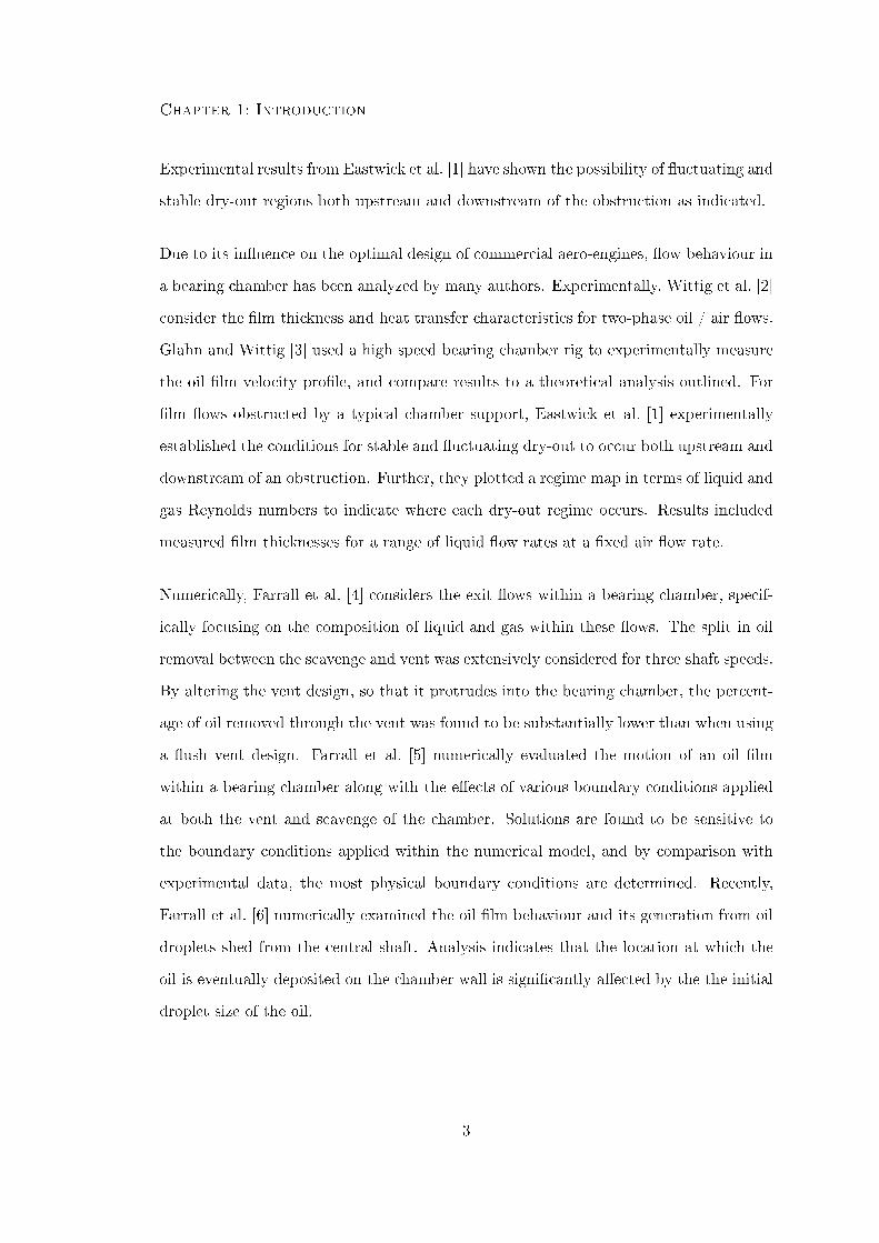
Experimental results from Eastwick et al. [1] have shown the possibility of uctuating and
stable dry-out regions both upstream and downstream of the obstruction as indicated.
Due to its inuence on the optimal design of commercial aero-engines, ow behaviour in
a bearing chamber has been analyzed by many authors. Experimentally, Wittig et al. [2]
consider the lm thickness and heat transfer characteristics for two-phase oil / air ows.
Glahn and Wittig [3] used a high speed bearing chamber rig to experimentally measure
the oil lm velocity prole, and compare results to a theoretical analysis outlined. For
lm ows obstructed by a typical chamber support, Eastwick et al. [1] experimentally
established the conditions for stable and uctuating dry-out to occur both upstream and
downstream of an obstruction. Further, they plotted a regime map in terms of liquid and
gas Reynolds numbers to indicate where each dry-out regime occurs. Results included
measured lm thicknesses for a range of liquid ow rates at a xed air ow rate.
Numerically, Farrall et al. [4] considers the exit ows within a bearing chamber, specif-
ically focusing on the composition of liquid and gas within these ows. The split in oil
removal between the scavenge and vent was extensively considered for three shaft speeds.
By altering the vent design, so that it protrudes into the bearing chamber, the percent-
age of oil removed through the vent was found to be substantially lower than when using
a ush vent design. Farrall et al. [5] numerically evaluated the motion of an oil lm
within a bearing chamber along with the eects of various boundary conditions applied
at both the vent and scavenge of the chamber. Solutions are found to be sensitive to
the boundary conditions applied within the numerical model, and by comparison with
experimental data, the most physical boundary conditions are determined. Recently,
Farrall et al. [6] numerically examined the oil lm behaviour and its generation from oil
droplets shed from the central shaft. Analysis indicates that the location at which the
oil is eventually deposited on the chamber wall is signicantly aected by the the initial
droplet size of the oil.
3
Chapter 1: Introduction
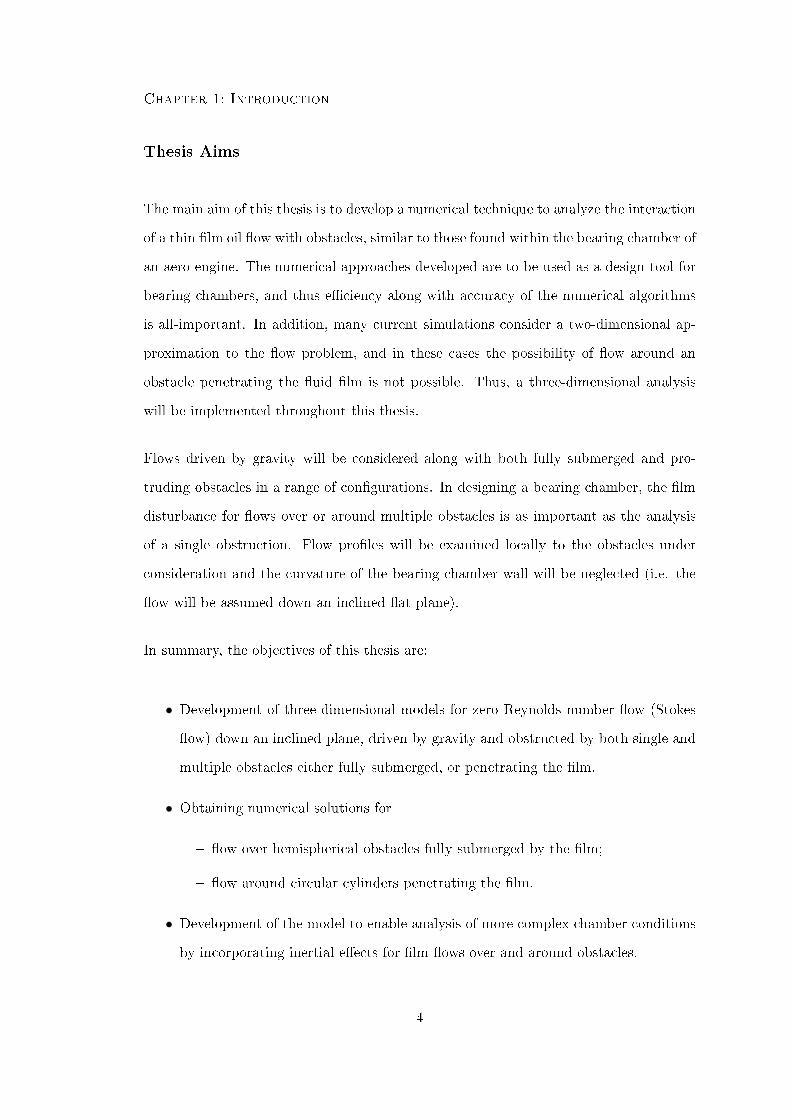
Thesis Aims
The main aim of this thesis is to develop a numerical technique to analyze the interaction
of a thin lm oil ow with obstacles, similar to those found within the bearing chamber of
an aero-engine. The numerical approaches developed are to be used as a design tool for
bearing chambers, and thus eciency along with accuracy of the numerical algorithms
is all-important. In addition, many current simulations consider a two-dimensional ap-
proximation to the ow problem, and in these cases the possibility of ow around an
obstacle penetrating the uid lm is not possible. Thus, a three-dimensional analysis
will be implemented throughout this thesis.
Flows driven by gravity will be considered along with both fully submerged and pro-
truding obstacles in a range of congurations. In designing a bearing chamber, the lm
disturbance for ows over or around multiple obstacles is as important as the analysis
of a single obstruction. Flow proles will be examined locally to the obstacles under
consideration and the curvature of the bearing chamber wall will be neglected (i.e. the
ow will be assumed down an inclined at plane).
In summary, the objectives of this thesis are:
• Development of three-dimensional models for zero Reynolds number ow (Stokes
ow) down an inclined plane, driven by gravity and obstructed by both single and
multiple obstacles either fully submerged, or penetrating the lm.
• Obtaining numerical solutions for
ow over hemispherical obstacles fully submerged by the lm;
ow around circular cylinders penetrating the lm.
• Development of the model to enable analysis of more complex chamber conditions
by incorporating inertial eects for lm ows over and around obstacles.
4

Chapter 1: Introduction
1.1 Literature Overview
Free surface lm ows occur regularly during coating and cooling processes in a wide
range of industrial applications, and as such are considered extensively by a range of
authors. This literature review is divided into two sections, initially giving an overview
of experimental work, providing an understanding of the uid dynamics, and the physical
eects with respect to the free surface and geometry within the ow problem. The nal
section of the literature review considers the numerical analysis of free surface lm ows,
relating the solutions obtained within the literature to the experimental results previously
discussed.
1.1.1 Physical Observation Of Film Flows
Experimental analysis give an important insight into the physical eects caused by lm
ows in a range of problems, with results allowing analysis of ow solutions and the
validation of numerical solutions.
Film ows over heterogeneously heated surfaces have been considered by a wide range of
authors, examining the eects of heat exchange between the wall and a uid lm. Kabov
[7] considered lm ow falling freely down a vertical plane over a local heat source of
two dierent lengths. When the longer heated regions were considered, instabilities in
the uid lm were formed, and the potential for dry patches on the lower part of the
heater found. This analysis of gravity driven lm ow down a vertical plane and over a
local heating unit was extended by Kabov and Marchuk [8]. Temperature gradients on
the lm surface were recorded, along with lm disturbances caused by the heating unit.
The breakdown of the lm is extensively analyzed for a range of Reynolds numbers,
with anything from one to three horseshoe shape lm deformations formed for the
dierent Reynolds numbers and heat ux densities considered. Recently, Kabov et al.
[9] reconsidered the falling liquid lm down a vertical, locally heated plane. Methods for
5
Chapter 1: Introduction
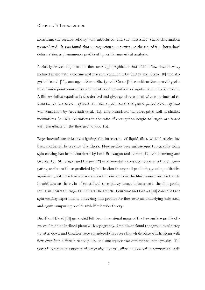
measuring the surface velocity were introduced, and the `horseshoe shape deformation
reconsidered. It was found that a stagnation point exists at the top of the horseshoe
deformation, a phenomenon predicted by earlier numerical analysis.
A closely related topic to lm ow over topographies is that of lm ow down a wavy
inclined plane with experimental research conducted by Shetty and Cerro [10] and Ar-
gyriadi et al. [11], amongst others. Shetty and Cerro [10] considers the spreading of a
uid from a point source over a range of periodic surface corrugations on a vertical plane.
A lm evolution equation is also derived and gives good agreement with experimental re-
sults for transverse corrugations. Further experimental analysis of periodic corrugations
was considered by Argyriadi et al. [11], who considered the corrugated wall at shallow
inclinations (< 15o). Variations in the ratio of corrugation height to length are tested
with the eects on the ow prole reported.
Experimental analysis investigating the interaction of liquid lms with obstacles has
been conducted by a range of authors. Flow proles over microscopic topography using
spin coating has been considered by both Stillwagon and Larson [12] and Peurrung and
Graves [13]. Stillwagon and Larson [12] experimentally consider ow over a trench, com-
paring results to those predicted by lubrication theory and producing good quantitative
agreement, with the free surface shown to form a dip as the lm passes over the trench.
In addition as the ratio of centrifugal to capillary forces is increased, the lm prole
forms an upstream ridge as it enters the trench. Peurrung and Graves [13] continued the
spin coating experiments, analyzing lm proles for ow over an underlying substrate,
and again comparing results with lubrication theory.
Decré and Baret [14] generated full two-dimensional maps of the free-surface prole of a
water lm on an inclined plane with topography. One-dimensional topographies of a step
up, step down and trenches were considered that cross the whole plate width, along with
ow over four dierent rectangular, and one square two-dimensional topography. The
case of ow over a square is of particular interest, allowing qualitative comparison with
6

Chapter 1: Introduction
numerical results considered in the following section. The ow prole exhibits a typical
horseshoe disturbance of a large upstream peak before the obstacle, decaying around
the obstruction, and returning to the undisturbed lm height further downstream.
The experimental study of the onset of dry-out in a lm has been considered by Shiralkar
and Lahey [15] and Eastwick et al. [1] amongst others. Shiralkar and Lahey [15], con-
sidered two-phase air-water ow to assess problems in nuclear reactors upstream of ow
obstacles. Both rectangular and cylindrical obstructions were used in the experiment and
their eects discussed. More recently, Eastwick et al. [1] considered lm ows around
bearing chamber supports. This paper focused on the determination of the conditions
necessary for dry-out to occur, both upstream and downstream of an obstacle using a
water-glycerol liquid and shearing air ow. Both studies [15] and [1] consider the eects
of varying the ow rate of the shearing air ow over the liquid lm. Shiralkar and Lahey
[15] observed two types of dry-out, which they categorized as Type I and Type II. Type
I occur upstream of the obstacle, and Type II is located behind the obstacle. Eastwick
et al. [1] extended these denitions of Type I and Type II dry-out to cover both stable
and uctuating dry-outs. This paper concluded with a regime map of dry-out condi-
tions for both the liquid and air Reynolds numbers. Although numerical formulations
presented in this thesis are not looking to capture the occurrence of dry-out, regions of
minimum lm depth are identied.
1.1.2 Numerical Simulation Of Film Flows
The industrial processes in which lm ows occur are often complex, with hostile en-
vironments, and thus the cost and time involved with obtaining accurate experimental
results is prohibitive. Numerical simulations of these complex lm ows are an important
design tool for optimization of industrial processes.
Numerical models are used to describe the dynamics of liquid lms falling down a vertical
plane and under the action of gravity when subjected to a local heat source. Skotheim
7
Chapter 1: Introduction
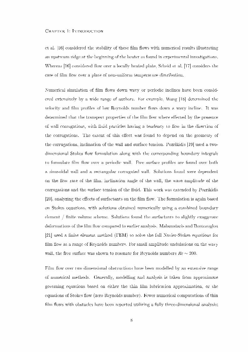
et al. [16] considered the stability of these lm ows with numerical results illustrating
an upstream ridge at the beginning of the heater as found in experimental investigations.
Whereas [16] considered ow over a locally heated plate, Scheid et al. [17] considers the
case of lm ow over a plate of non-uniform temperature distribution.
Numerical simulation of lm ows down wavy or periodic inclines have been consid-
ered extensively by a wide range of authors. For example, Wang [18] determined the
velocity and lm proles of low Reynolds number ows down a wavy incline. It was
determined that the transport properties of the lm ow where eected by the presence
of wall corrugations, with uid particles having a tendency to ow in the direction of
the corrugations. The extent of this eect was found to depend on the geometry of
the corrugations, inclination of the wall and surface tension. Pozrikidis [19] used a two-
dimensional Stokes ow formulation along with the corresponding boundary integrals
to formulate lm ow over a periodic wall. Free surface proles are found over both
a sinusoidal wall and a rectangular corrugated wall. Solutions found were dependent
on the ow rate of the lm, inclination angle of the wall, the wave amplitude of the
corrugations and the surface tension of the uid. This work was extended by Pozrikidis
[20], analyzing the eects of surfactants on the lm ow. The formulation is again based
on Stokes equations, with solutions obtained numerically using a combined boundary
element / nite volume scheme. Solutions found the surfactants to slightly exaggerate
deformations of the lm ow compared to earlier analysis. Malamataris and Bontozoglou
[21] used a nite element method (FEM) to solve the full Navier-Stokes equations for
lm ow at a range of Reynolds numbers. For small amplitude undulations on the wavy
wall, the free surface was shown to resonate for Reynolds numbers Re ∼ 200.
Film ow over two-dimensional obstructions have been modelled by an extensive range
of numerical methods. Generally, modelling and analysis is taken from approximate
governing equations based on either the thin lm lubrication approximation, or the
equations of Stokes ow (zero Reynolds number). Fewer numerical computations of thin
lm ows with obstacles have been reported utilizing a fully three-dimensional analysis;
8
Chapter 1: Introduction
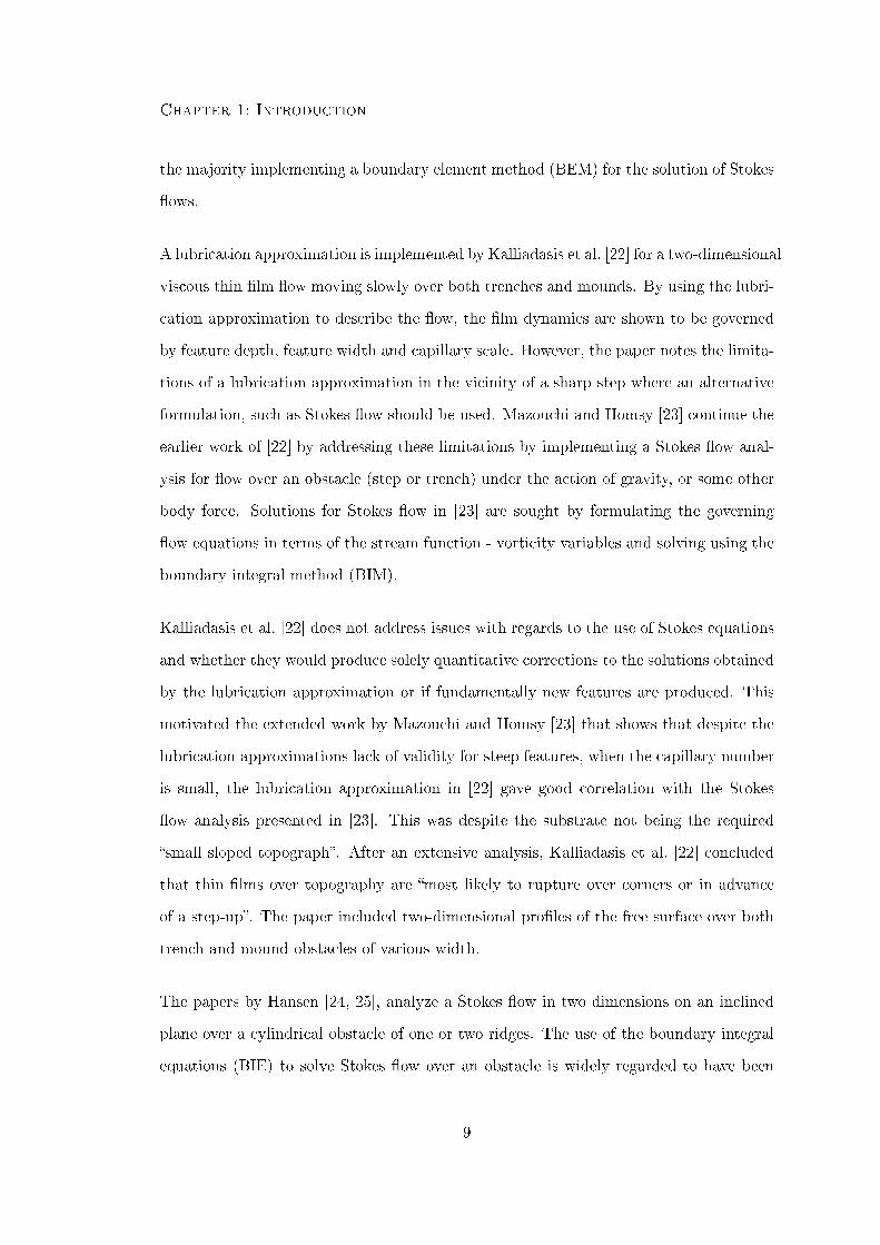
the majority implementing a boundary element method (BEM) for the solution of Stokes
ows.
A lubrication approximation is implemented by Kalliadasis et al. [22] for a two-dimensional
viscous thin lm ow moving slowly over both trenches and mounds. By using the lubri-
cation approximation to describe the ow, the lm dynamics are shown to be governed
by feature depth, feature width and capillary scale. However, the paper notes the limita-
tions of a lubrication approximation in the vicinity of a sharp step where an alternative
formulation, such as Stokes ow should be used. Mazouchi and Homsy [23] continue the
earlier work of [22] by addressing these limitations by implementing a Stokes ow anal-
ysis for ow over an obstacle (step or trench) under the action of gravity, or some other
body force. Solutions for Stokes ow in [23] are sought by formulating the governing
ow equations in terms of the stream function - vorticity variables and solving using the
boundary integral method (BIM).
Kalliadasis et al. [22] does not address issues with regards to the use of Stokes equations
and whether they would produce solely quantitative corrections to the solutions obtained
by the lubrication approximation or if fundamentally new features are produced. This
motivated the extended work by Mazouchi and Homsy [23] that shows that despite the
lubrication approximations lack of validity for steep features, when the capillary number
is small, the lubrication approximation in [22] gave good correlation with the Stokes
ow analysis presented in [23]. This was despite the substrate not being the required
small sloped topograph. After an extensive analysis, Kalliadasis et al. [22] concluded
that thin lms over topography are most likely to rupture over corners or in advance
of a step-up. The paper included two-dimensional proles of the free surface over both
trench and mound obstacles of various width.
The papers by Hansen [24, 25], analyze a Stokes ow in two dimensions on an inclined
plane over a cylindrical obstacle of one or two ridges. The use of the boundary integral
equations (BIE) to solve Stokes ow over an obstacle is widely regarded to have been
9
Chapter 1: Introduction
pioneered in [24, 25]. The BIE is formulated in terms of the stream function and the
system solved for the free surface position and any unknown eld variables. Free surface
proles are shown for a range of values of surface tension. For the case of the single
obstacle in [24] velocity on the free surface and tangential stress on the obstacle surface
are also shown.
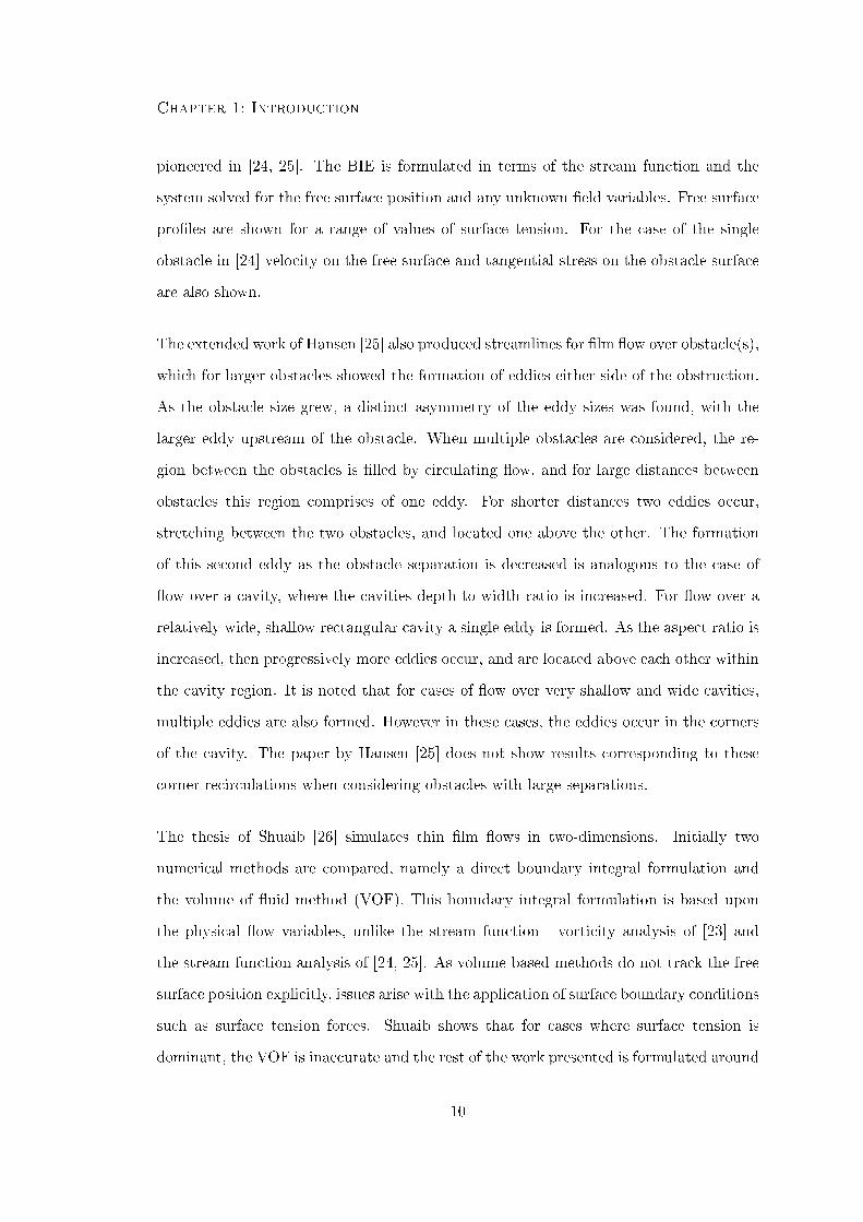
The extended work of Hansen [25] also produced streamlines for lm ow over obstacle(s),
which for larger obstacles showed the formation of eddies either side of the obstruction.
As the obstacle size grew, a distinct asymmetry of the eddy sizes was found, with the
larger eddy upstream of the obstacle. When multiple obstacles are considered, the re-
gion between the obstacles is lled by circulating ow, and for large distances between
obstacles this region comprises of one eddy. For shorter distances two eddies occur,
stretching between the two obstacles, and located one above the other. The formation
of this second eddy as the obstacle separation is decreased is analogous to the case of
ow over a cavity, where the cavities depth-to-width ratio is increased. For ow over a
relatively wide, shallow rectangular cavity a single eddy is formed. As the aspect ratio is
increased, then progressively more eddies occur, and are located above each other within
the cavity region. It is noted that for cases of ow over very shallow and wide cavities,
multiple eddies are also formed. However in these cases, the eddies occur in the corners
of the cavity. The paper by Hansen [25] does not show results corresponding to these
corner recirculations when considering obstacles with large separations.
The thesis of Shuaib [26] simulates thin lm ows in two-dimensions. Initially two
numerical methods are compared, namely a direct boundary integral formulation and
the volume of uid method (VOF). This boundary integral formulation is based upon
the physical ow variables, unlike the stream function - vorticity analysis of [23] and
the stream function analysis of [24, 25]. As volume based methods do not track the free
surface position explicitly, issues arise with the application of surface boundary conditions
such as surface tension forces. Shuaib shows that for cases where surface tension is
dominant, the VOF is inaccurate and the rest of the work presented is formulated around
10

Chapter 1: Introduction
the BEM. The ow was assumed to be governed by the two-dimensional Stokes ow
equations. Constant shear stress has been applied to the thin lm and results produced
for lm ow down an inclined plane, ow over a rectangular cavity, and ow into an
outlet. For more realistic calculations, variable shear stress was used to recalculate
results for some of the previous scenarios. Finally the dual reciprocity method (DRM)
was implemented to extend the Stokes approximation to include inertia eects.
A steady, three-dimensional thin viscous liquid lm driven by gravity down an inclined
plane and over small topographies was considered by Hayes et al. [27] and Gaskell et al.
[28]. Both formulations are based on the lubrication approximation, with Hayes et al. [27]
deriving a single linear inhomogeneous evolution equation and obtaining the disturbed
free surface prole by formulating the appropriate Green's function. Hayes et al. [27]
consider an obstacle based on the dirac delta distribution, a point defect on the inclined
plane, despite the lubrication approximation not being directly applicable in this case
(as acknowledged by the authors). Results using this lubrication approximation are
reported to give qualitatively similar results to the Stokes ow analysis of Pozrikidis
and Thoroddsen [29] for ow over a spherical obstacle. The accuracy of modelling lm
ows over steep sided topographies using the lubrication approximation was considered
by Gaskell et al. [28] by comparison of results with solutions to the full Navier-Stokes
equations found using a nite element method. Solutions produced by the two methods
reported good agreement. Thin lm ows over both single and multiple obstacles using
the lubrication approximation was considered by Lee et al. [30]. Film proles for a single
square, diamond and circular trench were all produced along with solution of the complex
multiple obstacle conguration of a central diamond trench with two circular trenches
downstream and two circular struts upstream.
Due to the added complexity in solving the full three-dimensional ow problem, restricted
approaches are available for analysis, with a lubrication approximation the most popular
technique. However, due to the additional simplication, problems arise with validity of
this assumption where the ow proles become steep. This problem is not present with
11
Chapter 1: Introduction
a Stokes ow analysis but such analysis are not yet well developed.
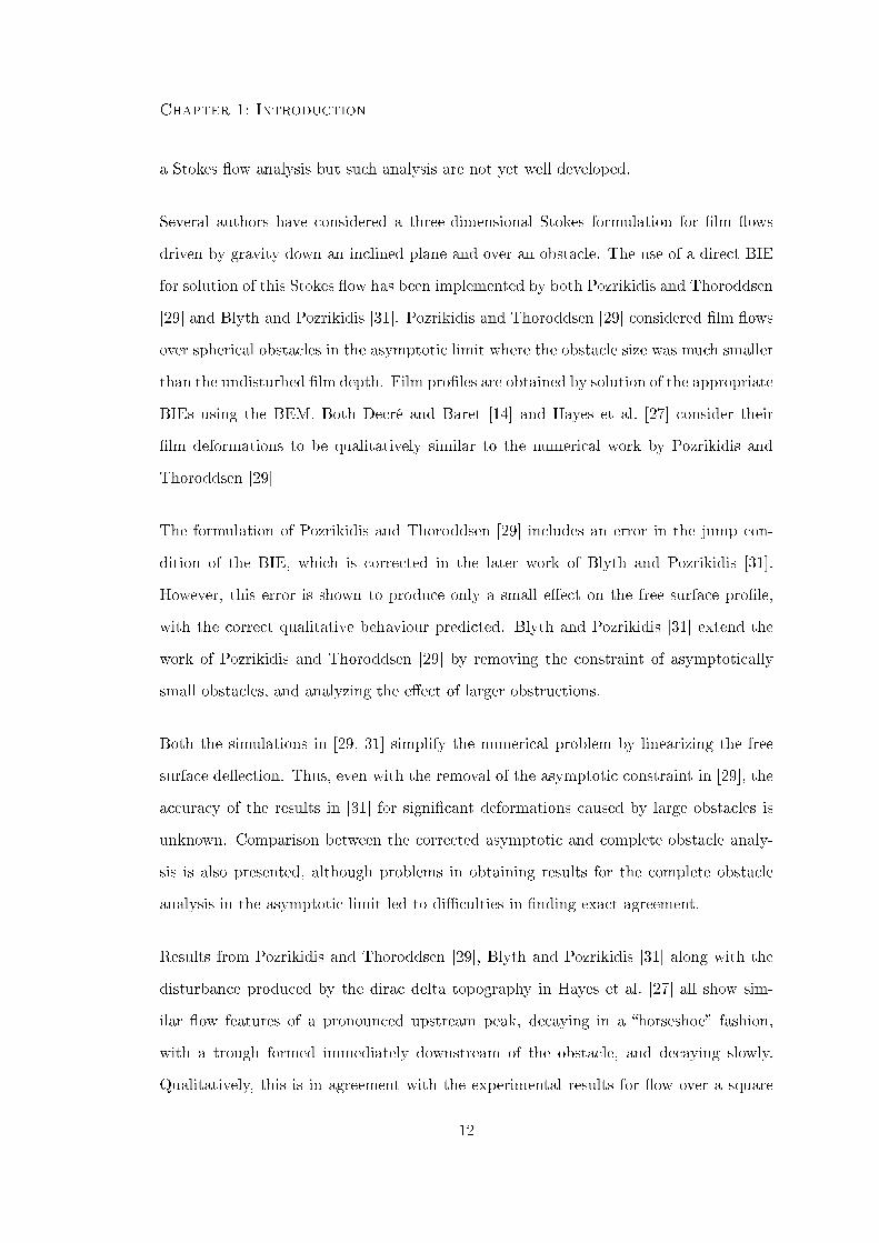
Several authors have considered a three-dimensional Stokes formulation for lm ows
driven by gravity down an inclined plane and over an obstacle. The use of a direct BIE
for solution of this Stokes ow has been implemented by both Pozrikidis and Thoroddsen
[29] and Blyth and Pozrikidis [31]. Pozrikidis and Thoroddsen [29] considered lm ows
over spherical obstacles in the asymptotic limit where the obstacle size was much smaller
than the undisturbed lm depth. Film proles are obtained by solution of the appropriate
BIEs using the BEM. Both Decré and Baret [14] and Hayes et al. [27] consider their
lm deformations to be qualitatively similar to the numerical work by Pozrikidis and
Thoroddsen [29]
The formulation of Pozrikidis and Thoroddsen [29] includes an error in the jump con-
dition of the BIE, which is corrected in the later work of Blyth and Pozrikidis [31].
However, this error is shown to produce only a small eect on the free surface prole,
with the correct qualitative behaviour predicted. Blyth and Pozrikidis [31] extend the
work of Pozrikidis and Thoroddsen [29] by removing the constraint of asymptotically
small obstacles, and analyzing the eect of larger obstructions.
Both the simulations in [29, 31] simplify the numerical problem by linearizing the free
surface deection. Thus, even with the removal of the asymptotic constraint in [29], the
accuracy of the results in [31] for signicant deformations caused by large obstacles is
unknown. Comparison between the corrected asymptotic and complete obstacle analy-
sis is also presented, although problems in obtaining results for the complete obstacle
analysis in the asymptotic limit led to diculties in nding exact agreement.
Results from Pozrikidis and Thoroddsen [29], Blyth and Pozrikidis [31] along with the
disturbance produced by the dirac delta topography in Hayes et al. [27] all show sim-
ilar ow features of a pronounced upstream peak, decaying in a horseshoe fashion,
with a trough formed immediately downstream of the obstacle, and decaying slowly.
Qualitatively, this is in agreement with the experimental results for ow over a square
12
Chapter 1: Introduction
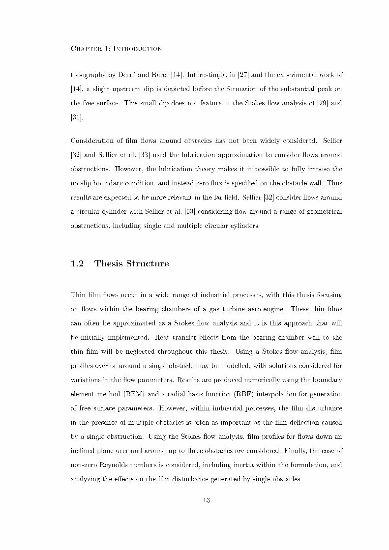
topography by Decré and Baret [14]. Interestingly, in [27] and the experimental work of
[14], a slight upstream dip is depicted before the formation of the substantial peak on
the free surface. This small dip does not feature in the Stokes ow analysis of [29] and
[31].
Consideration of lm ows around obstacles has not been widely considered. Sellier
[32] and Sellier et al. [33] used the lubrication approximation to consider ows around
obstructions. However, the lubrication theory makes it impossible to fully impose the
no-slip boundary condition, and instead zero ux is specied on the obstacle wall. Thus
results are expected to be more relevant in the far eld. Sellier [32] consider ows around
a circular cylinder with Sellier et al. [33] considering ow around a range of geometrical
obstructions, including single and multiple circular cylinders.
1.2 Thesis Structure
Thin lm ows occur in a wide range of industrial processes, with this thesis focusing
on ows within the bearing chambers of a gas turbine aero-engine. These thin lms
can often be approximated as a Stokes ow analysis and it is this approach that will
be initially implemented. Heat transfer eects from the bearing chamber wall to the
thin lm will be neglected throughout this thesis. Using a Stokes ow analysis, lm
proles over or around a single obstacle may be modelled, with solutions considered for
variations in the ow parameters. Results are produced numerically using the boundary
element method (BEM) and a radial basis function (RBF) interpolation for generation
of free surface parameters. However, within industrial processes, the lm disturbance
in the presence of multiple obstacles is often as important as the lm deection caused
by a single obstruction. Using the Stokes ow analysis, lm proles for ows down an
inclined plane over and around up to three obstacles are considered. Finally, the case of
non-zero Reynolds numbers is considered, including inertia within the formulation, and
analyzing the eects on the lm disturbance generated by single obstacles.
13

Chapter 1: Introduction
This chapter has considered an overview of the literature discussing the physical be-
haviour of lm ows along with their numerical simulation, and below a detailed de-
scription of the following chapters of this thesis is presented.
Chapter 2 overviews the theory of viscous ows, and the formulation of the corresponding
boundary integral equations (BIEs). The end of chapter 2 discusses solution of the
integral equations by the BEM, a numerical scheme. In addition, thin lms are often
dominated by surface tension eects, and thus for accurate evaluation of these forces,
an accurate representation of the free surface and its derivatives are required. This is
achieved by using a radial basis function (RBF) interpolation and more details are given
in chapter 3. The extension of Stokes ow analysis to the full Navier-Stokes solutions
for ows at nite Reynolds number is modelled in chapter 7 and also requires RBF
interpolations.
Chapter 4 considers Stokes ow down an inclined plane, and driven by gravity over a sin-
gle obstacle. Duplication of the methods introduced in the publications of Pozrikidis and
Thoroddsen [29] and Blyth and Pozrikidis [31] provides an initial milestone to generate
numerical codes and provide a base case for later qualitative comparisons. Assumptions
of small free surface deections are implemented by both [29] and [31] with [29] also
imposing the constraint of asymptotically small obstacles. The small free surface deec-
tion assumption allows linearization of the unknown free surface location, and the lm
prole can be found directly by the solution of a system of equations. Development of
the analysis from [31] is aimed at obtaining solution methods for modelling ow over
more general obstacles and ow conditions, with the model developed to relax the small
deection restrictions of the governing equations. The removal of the small free surface
deection requires solution of a non-linear problem, and an iterative solution technique
has been developed.
A further extension to lm ow over a single obstacle considers the lm disturbance
for ow over multiple obstacles located close to one another. The interaction between
14
Chapter 1: Introduction
multiple obstacles fully submerged by the lm is considered in chapter 5. Two and three
hemispheres in a range of relative locations are analyzed with the eects of the wake
from one obstacle, on the lm deformation caused by a subsequent obstacle discussed.
In addition, eects of ow parameters on the lm disturbance are considered.
Thin lm ows around obstacles have been less widely considered in the literature, with
Sellier [32] and Sellier et al. [33] the only reported works. However in using the lubri-
cation theory, the no slip boundary condition on the obstacle wall is not fully imposed,
with no ux specied instead. By using a Stokes ow analysis, lm ows around ob-
structions using the full no-slip boundary condition on the wetted obstacle surface can be
accurately modelled. The consideration of both single and multiple obstacles that pen-
etrate the free surface are considered in chapter 6. For this analysis the incorporation
of a contact line condition in the problem formulation is required. This is a non-trivial
extension to the ow over analysis, and the contact angle at the contact line of the lm
is constrained using the RBF interpolation of the free surface. Circular cylinders are
considered throughout, again with the relative positioning of obstacles assessed. The
incorporation of the additional contact line constraint yields the possibility of multiple
solutions. This is where for identical ow parameters, and far eld conditions, the prole
can exist both over, or around an identical obstacle.
The Reynolds number of thin lm ows is often small and the Stokes ow assumption
implemented up until Chapter 6 is often an appropriate approximation. However, even
at low Reynolds numbers, the eects of inertia on the lm prole may be signicant.
Chapter 7 considers the eects of the convective term from the Navier-Stokes equations
on the lm prole. An ecient numerical algorithm is developed for incorporating inertia
eects, with the case of a three-dimensional lid driven cavity used to benchmark the
algorithms. Incorporation of these numerical techniques into the lm model allows the
eects of low, nite Reynolds number to be considered.
In the nal chapter, development of the theory and numerical aspects of this work are
15

Chapter 1: Introduction
reviewed, along with a discussion of the key results obtained. A particularly important
aspect is the new insight into thin lm ows around obstacles. Future developments and
applications of this work are also discussed.
16
Chapter 2
Viscous Flows
This chapter considers the development of Stokes ow as an approximation to the Navier-
Stokes equations for viscous uid ow. The fundamental solution will be used to form the
boundary integral equation (BIE) that will be the basis of the numerical solver utilizing
the boundary element method (BEM). Initially, the Navier-Stokes equations are non-
dimensionalized, and used to obtain the governing equations of Stokes ow (see § 2.1),
and similar derivations are shown in [3437]. The use of a direct formulation of the BIEs
for Stokes ow is then analyzed in § 2.3 with the BEM, a numerical technique used to
obtain solutions of the BIEs discussed in § 2.4
2.1 Introduction To Viscous Flows
The ow of an incompressible Newtonian uid under the inuence of a body force is
governed by the Navier-Stokes equations, a vector equation for the conservation of
momentum (2.1.1), and the scalar continuity equation for the conservation of mass
(2.1.2). Although not presented here, full derivations of these equations can be found in
[34, 35, 38, 39]. For a uid whose motion is dominated by viscous eects, the Navier-
Stokes equations can be approximated by the simpler Stokes equations using certain
assumptions which will be discussed in some detail.
17

Chapter 2: Viscous Flows
Non-dimensionalizing the Navier-Stokes equation allows simplication by means of a
constraint on the non-dimensional quantity - the Reynolds number, Re. The Reynolds
number is a representative value of the ratio of inertia forces to viscous forces acting
within the uid ow, and for the case of low Re, i.e. Re 1 uid inertia forces are
negligible compared to the viscous forces. The viscous forces are balanced with the
remaining terms in the Navier-Stokes equations, i.e. pressure and external body forces.
The main benet of this simplication is the removal of the non-linear term from (2.1.1)
and results in Stokes equation. The equation for mass conservation (2.1.2) is unaltered.
Typically, the Reynolds number is generally small when either the characteristic velocity
or length scale of the ow is very small or the kinematic viscosity of the uid is very
large. Correspondingly these ows are also referred to as creeping ows or slow ows,
and are associated with the limit of the Reynolds number tending to zero.
Stokes Flow
Consider the ow of an incompressible Newtonian uid under the inuence of a gravita-
tional body force g, with velocity u = (u1, u2, u3) , pressure p, density ρ, and dynamic vis-
cosity µ. Over bars are used to denote dimensional quantities, with the non-dimensional
variables plain. The uid ow is governed by the Navier-Stokes equations (2.1.1) and
the continuity equation (2.1.2),
ρ
(∂u∂t
+ u · ∇u)
= −∇p+ µ∇2u + ρg, (2.1.1)
∇ · u = 0. (2.1.2)
Gravitational body forces are conservative, and thus the gravitational force can be rewrit-
ten as the gradient of a second function, i.e. g = ∇G. As such the gravitational body
force can be combined with the pressure term from the Navier-Stokes equations, produc-
ing,
ρ
(∂u∂t
+ u · ∇u)
= −∇pmod + µ∇2u (2.1.3)
18
Chapter 2: Viscous Flows
where pmod = p − ρG. For a uid whose motion is dominated by viscous eects, the
Navier-Stokes equations can be reduced to the simpler Stokes equations using certain
assumptions which will be discussed in some detail.
The equations for a Stokes ow subject to gravitational body forces are obtained by
simplifying the full Navier-Stokes equations (2.1.3) for an incompressible uid. The
derivation in this section recreates in full detail that presented in [34]. To proceed, ow
quantities in equation (2.1.3) are non-dimensionalized based on representative values of
velocity U , length L and time T for the ow. In cases of thin lms the length scale L
is often taken as the characteristic thickness of the lm. A representative pressure is
obtained by scaling the pressure term with the dominant viscous term in (2.1.3). Hence
the following dimensionless variables can now be dened,
u ≡ uU, x ≡ x
L, ∇ ≡ L∇, t ≡ t
T, pmod ≡ pmodL
µU. (2.1.4)
Substituting expressions (2.1.4) into (2.1.3) yields the non-dimensional equations for
mass conservation and Navier-Stokes,
L2
Tν
∂u∂t
+LU
νu · ∇u = −∇pmod +∇2u, (2.1.5)
U
L∇ · u = 0, (2.1.6)
where the kinematic viscosity is given by ν where (µ = νρ).
Two dimensionless parameters are now introduced. The rst is the Reynolds number,
denoted Re, which expresses the ratio between inertia and viscous forces and is given by
Re =LU
ν. (2.1.7)
The next is the unsteadiness parameter and represents the ratio of inertial acceleration
body forces and the viscous forces. It is denoted by β and is expressed as,
β =L2
νT= Re
L
UT, (2.1.8)
and in cases where the typical velocity, length and time scales are interlinked (i.e. U =
LT ), β reduces to the Reynolds number Re.
19
Chapter 2: Viscous Flows
Using dimensionless parameters (2.1.7) - (2.1.8), (2.1.5) and (2.1.6) reduce to
β∂u∂t
+ Re u · ∇u = −∇p+∇G+∇2u, (2.1.9)
∇ · u = 0. (2.1.10)
For steady ows, or ows with a relatively long time scale, the frequency parameter β
is approximated by β 1 and the time derivative term in (2.1.9) can be neglected,
resulting in the equations for steady Navier-Stokes ow,
Re u · ∇u = −∇p+∇G+∇2u. (2.1.11)
In terms of the Reynolds number there are three broad cases,
• Re 1 - Inertia forces are dominated by viscous forces and pressure forces.
• Re ∼ O(1) - Inertial, viscous and pressure forces are all of the same magnitude and
thus are all equally important to the motion of the uid.
• Re 1 - Viscous forces are dominated by inertia and pressure forces. Note for
consistency in this case, the assumed scaling for pressure would be changed to
balance the inertia terms.
Thus in the case of Re 1, (2.1.11) simplies to the steady Stokes equation,
−∇p+∇G+∇2u = 0. (2.1.12)
2.2 An Overview Of The Boundary Integral Formulation
A wide range of engineering problems are governed by linear partial dierential equations
(PDEs) which require solving. The governing equation can be re-written exactly as an
integral equation and is often referred to as the boundary integral equation (BIE). The
20
Chapter 2: Viscous Flows
BIE is obtained by using the corresponding Green's function appropriate for the case of
interest. This imposes restrictions due to the diculty in nding the Green's function
required for creating the BIE from the original PDE.
The BIE formulations can take two forms, direct and indirect. The indirect approach
formulates integral equations in terms of ctitious sources with no physical meaning. The
integral equation is solved for these ctitious source densities and physical variables can
be computed afterwards. The need to introduce the ctitious densities can be eliminated
by use of a Direct approach which formulates the integral equations in terms of the
physical quantities (for example tractions and velocities). Solely the direct formulation
is focused on here and thus in future the distinction will not always be made.
For non-linear cases, the problem is formulated in terms of the boundary integrals cor-
responding to the linear case, with an additional domain integral incorporating the non-
linear term. Early works required the discretization of the full domain, eliminating one
of the major benets of the boundary integral formulation. More recent work has con-
sidered methods of keeping the boundary-only nature of the formulation, and details are
presented in chapter 7.
The boundary element method (BEM) is a numerical computational method used to
solve the BIE, by applying the specied boundary conditions and introducing three
approximations. Initially a geometric approximation is made, where the boundary is
discretized into a set of elements. The BIE is then re-written as the sum of the integrals
over each of the elements. The boundary distributions of the surface variables (i.e.
boundary tractions and velocities) are then approximated on each of the previously
dened boundary elements. Finally the integrals dened over each element are evaluated
by an appropriate numerical scheme. Values for the unknown surface variables can then
be found on the contours of the problem domain. Using the BIE and BEM again, these
surface values can be used to nd the values for the variables anywhere within the ow
domain.
21
Chapter 2: Viscous Flows
The major advantage of the BEM over volume-discretization methods such as the nite
element method (FEM) or nite volume method (FVM) is obvious, that only the bound-
ing surface requires discretization and the dimension of the solution space is reduced by
one when compared to the dimension of the physical variable space. For problems with
a solution domain with a large volume/surface ratio the BEM can oer signicant per-
formance advantages over volume-meshing based solution methods. However, one disad-
vantage of the BEM is its formation of fully populated matrices. Memory requirements
for BEM problems grow with the square of the number of elements, whereas for a typical
FEM analysis, the matrix is banded and the growth relationship linear. Additionally, for
cases where surface properties (e.g. surface tension) are important, the BIE formulation
can oer signicant improvement in accuracy when compared with the volume of uid
(VOF) method, a more typical numerical scheme for uid problems. More details in the
comparison of these two methods was conducted in the PhD Thesis by Shuaib [26].
The following section gives a detailed account of the formation of the BIE for Stokes ow
using the direct formulation. This is followed by details of the BEM, describing typical
approximations that may be utilized in its application.
2.3 Direct Boundary Integral Equations For Stokes Flow
Formulation of the direct boundary integral equations (BIE) for Stokes ow requires the
Lorentz reciprocal identity, calculation of the relevant Green's functions and formulation
of the governing integral equations. Derivations of the direct BIE are produced in many
texts, for example [34, 35, 37]. For consistency, notation wherever possible is kept the
same as [34], however, the derivation shown throughout is non-dimensional.
22

Chapter 2: Viscous Flows
2.3.1 Derivation Of The Lorentz Reciprocal Relation
Stokes ow in the absence of gravitational body forces is given by (2.3.1)
−∇p+∇2u = 0. (2.3.1)
By dening the non-dimensional stress tensor σij as follows,
σij = −pδij +(∂ui∂xj
+∂uj∂xi
), (2.3.2)
the Stokes equation (2.3.1) can be rewritten as
∇ · σ = 0. (2.3.3)
Consider two solutions u, u′ corresponding to stress tensors σ, σ′ of a Stokes ow
governed by (2.3.3) and (2.1.10). Taking the inner product of u′ and the divergence of
the stress tensor ∇ · σ, and substituting (2.3.2) for the stress tensor yields,
u′j∂σij∂xi
=∂
∂xi(u′jσij)−
(−pδij +
(∂ui∂xj
+∂uj∂xi
))∂u′j∂xi
. (2.3.4)
By the standard properties of the Kronecker's delta function and noting that by mass
conservation∂u′i∂xi
= 0,
u′j∂σij∂xi
=∂
∂xi(u′jσij)−
(∂ui∂xj
+∂uj∂xi
)∂u′j∂xi
. (2.3.5)
Interchanging the ow solutions, i.e. u′ ↔ u and σ′ ↔ σ the following identity is
obtained,
uj∂σ′ij∂xi
=∂
∂xi(ujσ′ij)−
(∂u′i∂xj
+∂u′j∂xi
)∂uj∂xi
. (2.3.6)
The penultimate step of the derivation involves subtracting (2.3.6) from (2.3.5). By
manipulating the indices of the viscous term on the right hand side of (2.3.6), it can be
shown to cancel with the corresponding term in (2.3.5) to give,
u′j∂σij∂xi− uj
∂σ′ij∂xi
=∂
∂xi(u′jσij − ujσ′ij). (2.3.7)
23

Chapter 2: Viscous Flows
By the initial statement that both ows satisfy the equations of Stokes ow,
∇ · σ′ ≡∂σ′ij∂xi
= 0, ∇ · σ ≡ ∂σij∂xi
= 0, (2.3.8)
the expression (2.3.7) reduces to the Lorentz reciprocal relation,
∂
∂xi(u′jσij − ujσ′ij) = 0, (2.3.9)
or in vector notation
∇ · (u′ · σ − u · σ′) = 0. (2.3.10)
2.3.2 Fundamental Solutions And Their Properties
The analysis of Stokes ow involves two key terms, a fundamental solution and Green's
function. A fundamental solution of Stokes ow is one that satises the singularly forced
Stokes equation (2.3.11) or (2.3.12) and the continuity equation (2.1.10). A Green's
function for Stokes ow is a fundamental solution that also satises suitable boundary
conditions for the specic problem modelled. In three-dimensions, the singularly forced
Stokes equation is,
−∇p+∇2u + δ(x− x0)b = 0, (2.3.11)
or
∇ · σ + δ(x− x0)b = 0, (2.3.12)
where δ is Dirac's delta function, x0 is some arbitrary location of the singularity, x is
the eld point, and b is some constant vector. The fundamental solutions of Stokes ow
correspond to the solutions of (2.3.11) or (2.3.12) along with mass conservation (2.1.10)
and they describe the ow caused by a point force (or pole) at x0, with orientation and
strength given by b .
24

Chapter 2: Viscous Flows
Solutions of (2.3.11) or (2.3.12) are conventionally written in the form (see [34, 37]),
ui(x) =1
8πGij(x,x0)bj (2.3.13)
pi(x) =1
8πPj(x,x0)bj (2.3.14)
σik(x) =1
8πTijk(x,x0)bj (2.3.15)
Green's Function In Free-Space And Bounded Domains
The free-space Green's function (fundamental solution) for a three-dimensional Stokes
ow are well known, e.g.[34, 37], and are,
Gij(x) =δijr
+xixjr3
, (2.3.16)
Pj(x) = 2xir3, (2.3.17)
Tijk(x) = −6xixj xkr5
, (2.3.18)
where
x ≡ x− x0, r = |x|. (2.3.19)
The Green's function (2.3.16) corresponding to the velocity eld (2.3.13) is also referred
to as the Stokeslet. The choice of Green's functions for bounded and periodic domains
may involve requirements on the domain boundaries. For example, if for a given problem,
a section of boundary requires the uid velocity to be zero, then it is often convenient to
choose a Green's function that is also zero on this surface. The Lorentz-Blake Green's
functions can be used to model problems bounded by a plane wall with details given in
Appendix A.
Fundamental Solutions: Symmetry And Other Properties
Here the form of the fundamental solutions shown in equations (2.3.16) - (2.3.18) are
analyzed, with six symmetry relations or integral properties dened. Before proceeding
25

Chapter 2: Viscous Flows
Figure 2.1: Schematic of a typical domain for which the Green's functions are applied.
with the derivation of these properties an arbitrary control volume Vc , bounded by the
surface D is dened with the surface having unit normal vector n, pointing out of the
control volume Vc. For a detailed schematic see gure 2.1
(i) Due to the inherent symmetry of the stress tensor (σik = σki - see equation (2.3.2))
it is obvious that the corresponding fundamental solution will also have the sym-
metry property,
Tijk = Tkji. (2.3.20)
(ii) The fundamental solution associated with the velocity eld has symmetry property,
Gij(x,x0) = Gji(x0,x), (2.3.21)
and a proof is given in [37]. Hence a swap of the location of the eld point and
pole in conjunction with an exchange in the order of the indices is allowed.
(iii) By mass conservation, equation (2.1.10) must be satised and substituting from
(2.3.13) gives,
∇ ·G(x,x0) ≡ ∂Gij(x,x0)∂xi
= 0. (2.3.22)
Integration of (2.3.22) over the control volume Vc yields,∫Vc
∂Gij(x,x0)∂xi
dV (x) = 0, (2.3.23)
26

Chapter 2: Viscous Flows
and by applying the divergence theorem becomes,∫D
Gij(x,x0)ni(x)dS(x) = 0. (2.3.24)
(iv) Substituting equations (2.3.13) and (2.3.14) into (2.3.11) results in the relation,
− ∂
∂xi(Pj(x,x0)bj) +
∂2
∂xk∂xk(Gij(x,x0)bj) + 8πδ(x− x0)bi = 0. (2.3.25)
Introducing the Kronecker's delta function enables cancelling of the bj terms that
appear throughout the expression and yields the result,
−∂Pj(x,x0)∂xi
+∂2
∂xk∂xkGij(x,x0) + 8πδ(x− x0)δij = 0. (2.3.26)
(v) Substituting from (2.3.15) into (2.3.12) yields the relation,(∂Tkji(x,x0)
∂xk
)bj + 8πδ(x− x0)bi = 0. (2.3.27)
Switching the indices of the fundamental stress solution and repeating the previous
analysis by introducing the Kronecker's delta function and again cancelling the
terms bj , gives
∂Tijk(x,x0)∂xk
+ 8πδ(x− x0)δij = 0. (2.3.28)
Integrating (2.3.28) over the control volume Vc, yields∫Vc
∂Tijk(x,x0)∂xk
dV (x) = −8πδij∫Vc
δ(x− x0)dV (x), (2.3.29)
and applying the divergence theorem to the integral on the left hand side of (2.3.29)
gives,
− 18π
∫D
Tijk(x,x0)nk(x)dS(x) = δij
∫Vc
δ(x− x0)dV (x). (2.3.30)
By the properties of Dirac's delta function, the right hand side integral in (2.3.30)
is unity if x0 is contained in Vc and zero if x0 is outside of Vc. If x0 lies on the
locally smooth surface D (bounding Vc), then the integral equals a half. For a
27
Chapter 2: Viscous Flows
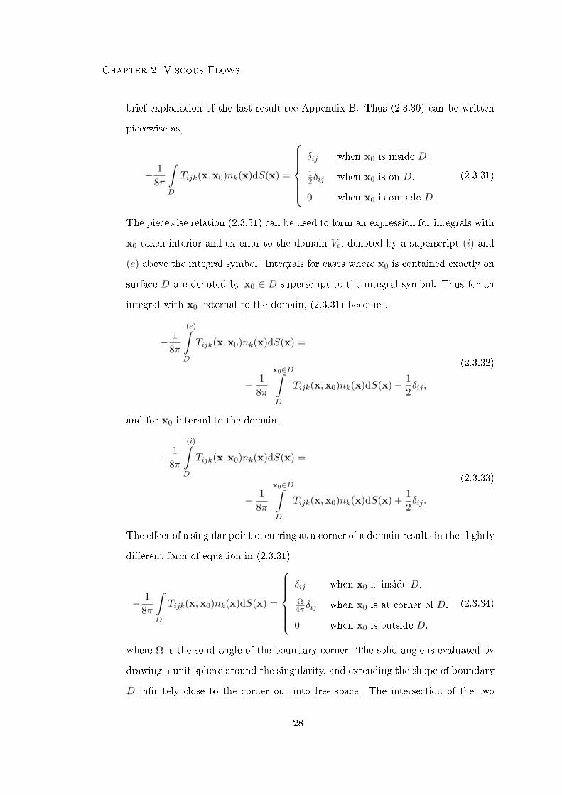
brief explanation of the last result see Appendix B. Thus (2.3.30) can be written
piecewise as,
− 18π
∫D
Tijk(x,x0)nk(x)dS(x) =
δij when x0 is inside D.
12δij when x0 is on D.
0 when x0 is outside D.
(2.3.31)
The piecewise relation (2.3.31) can be used to form an expression for integrals with
x0 taken interior and exterior to the domain Vc, denoted by a superscript (i) and
(e) above the integral symbol. Integrals for cases where x0 is contained exactly on
surface D are denoted by x0 ∈ D superscript to the integral symbol. Thus for an
integral with x0 external to the domain, (2.3.31) becomes,
− 18π
(e)∫D
Tijk(x,x0)nk(x)dS(x) =
− 18π
x0∈D∫D
Tijk(x,x0)nk(x)dS(x)− 12δij ,
(2.3.32)
and for x0 internal to the domain,
− 18π
(i)∫D
Tijk(x,x0)nk(x)dS(x) =
− 18π
x0∈D∫D
Tijk(x,x0)nk(x)dS(x) +12δij .
(2.3.33)
The eect of a singular point occurring at a corner of a domain results in the slightly
dierent form of equation in (2.3.31)
− 18π
∫D
Tijk(x,x0)nk(x)dS(x) =
δij when x0 is inside D.
Ω4π δij when x0 is at corner of D.
0 when x0 is outside D.
(2.3.34)
where Ω is the solid angle of the boundary corner. The solid angle is evaluated by
drawing a unit sphere around the singularity, and extending the shape of boundary
D innitely close to the corner out into free-space. The intersection of the two
28

Chapter 2: Viscous Flows
surfaces denes a contour on the sphere, whose area within the original domain
is the solid angle Ω. Note that Ω = 2π is eectively the earlier case of a locally
smooth boundary D, and Ω can take any value between 0 and 4π. The form of the
right hand side of (2.3.34) is also considered in Appendix B.
The corresponding equation to (2.3.32) when x0 is exterior to the domain D is,
− 18π
(e)∫D
Tijk(x,x0)nk(x)dS(x) =
− 18π
x0∈D∫D
Tijk(x,x0)nk(x)dS(x)− Ω4πδij ,
(2.3.35)
and when x0 is interior to the domain,
− 18π
(i)∫D
Tijk(x,x0)nk(x)dS(x) =
− 18π
x0∈D∫D
Tijk(x,x0)nk(x)dS(x) +(
1− Ω4π
)δij ,
(2.3.36)
corresponding to (2.3.33) for a smooth boundary.
(vi) The fundamental solution T is related to the fundamental solution for pressure P,
and velocity G , by substituting (2.3.13) - (2.3.15) into (2.3.2) to give,
18πTijk(x,x0)bj = − 1
8πPj(x,x0)δikbj
+1
8π
(∂Gij(x,x0)
∂xk+∂Gkj(x,x0)
∂xi
)bj .
(2.3.37)
Notice that for direct substitution, the indices j need to be changed to k in (2.3.2).
Cancelling wherever possible, the following relation (for which the symmetry con-
dition (i), clearly still holds) is obtained,
Tijk(x,x0) = −Pj(x,x0)δik +∂Gij(x,x0)
∂xk+∂Gkj(x,x0)
∂xi. (2.3.38)
29

Chapter 2: Viscous Flows
2.3.3 Derivation Of The Direct Boundary Integral Equations
The derivation of the direct BIEs for the velocity u of a three-dimensional Stokes ow is
shown below. Consider a specic Stokes ow of interest with velocity u and stress tensor
σ, satisfying (2.3.1) or (2.3.3), and dene the singularly forced Stokes ow satisfying
(2.3.11) or (2.3.12) as having solutions of the form shown in (2.3.39) - (2.3.41),
u′i(x) =1
8πGim(x,x0)bm, (2.3.39)
σ′ij(x) =1
8πTimj(x,x0)bm, (2.3.40)
∂σ′ij∂xi
= −δ(x− x0)bj , (2.3.41)
where b is some arbitrary constant vector and (2.3.39) - (2.3.40) are of similar form to
(2.3.13) and (2.3.15).
By equation (2.3.7) of the derivation of the Lorentz reciprocal relation,
∂
∂xi(u′jσij − ujσ′ij) = u′j
∂σij∂xi− uj
∂σ′ij∂xi
. (2.3.42)
The solution of the specic Stokes ow satises∂σij∂xi
= 0 and the scalar equation (2.3.42)
becomes,
∂
∂xi
(1
8πGjm(x,x0)bmσij(x)− uj(x)
18πTimj(x,x0)bm
)= um(x)δ(x−x0)bm,
(2.3.43)
or as b is arbitrary,
um(x)δ(x− x0) =
∂
∂xi
(1
8πGjm(x,x0)σij(x)− uj(x)
18πTimj(x,x0)
).
(2.3.44)
Introduce a control volume Vc such as in gure 2.1, that is bounded by a surface D
which has an outward unit normal vector n. Equation (2.3.44) can be integrated over
this volume and simplication made as the integral on the right hand side reduces to a
30
Chapter 2: Viscous Flows
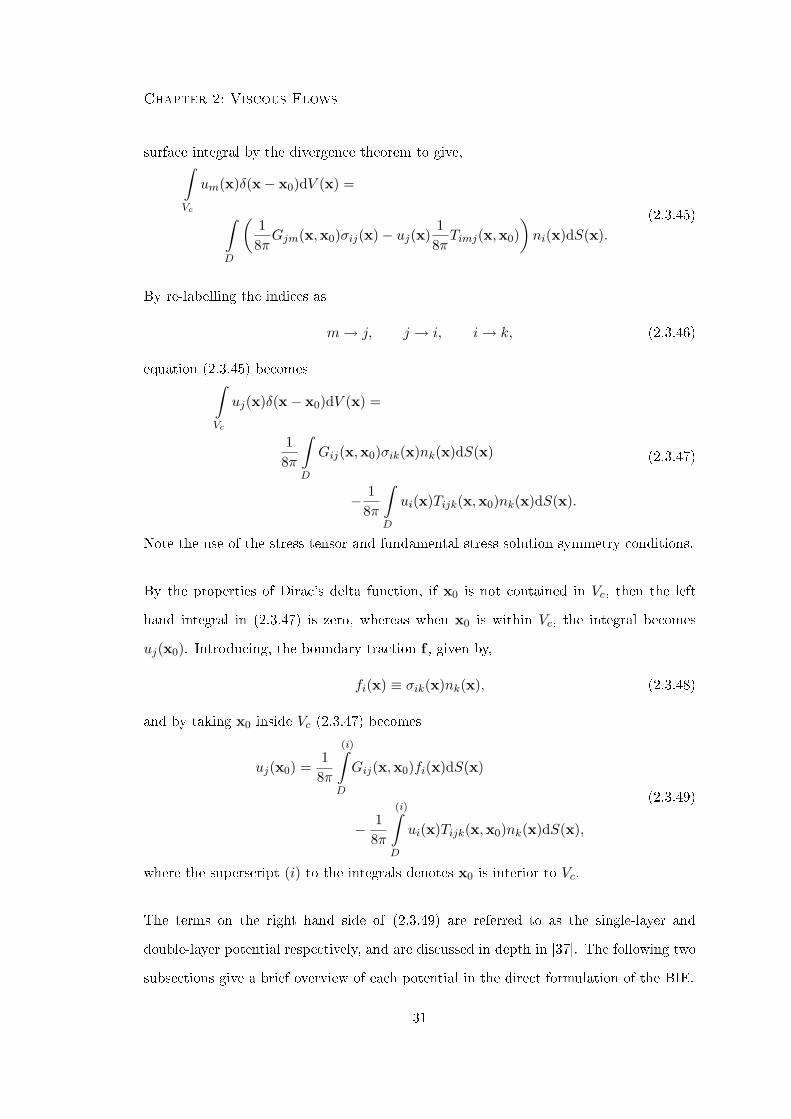
surface integral by the divergence theorem to give,∫Vc
um(x)δ(x− x0)dV (x) =
∫D
(1
8πGjm(x,x0)σij(x)− uj(x)
18πTimj(x,x0)
)ni(x)dS(x).
(2.3.45)
By re-labelling the indices as
m→ j, j → i, i→ k, (2.3.46)
equation (2.3.45) becomes∫Vc
uj(x)δ(x− x0)dV (x) =
18π
∫D
Gij(x,x0)σik(x)nk(x)dS(x)
− 18π
∫D
ui(x)Tijk(x,x0)nk(x)dS(x).
(2.3.47)
Note the use of the stress tensor and fundamental stress solution symmetry conditions.
By the properties of Dirac's delta function, if x0 is not contained in Vc, then the left
hand integral in (2.3.47) is zero, whereas when x0 is within Vc, the integral becomes
uj(x0). Introducing, the boundary traction f , given by,
fi(x) ≡ σik(x)nk(x), (2.3.48)
and by taking x0 inside Vc (2.3.47) becomes
uj(x0) =1
8π
(i)∫D
Gij(x,x0)fi(x)dS(x)
− 18π
(i)∫D
ui(x)Tijk(x,x0)nk(x)dS(x),
(2.3.49)
where the superscript (i) to the integrals denotes x0 is interior to Vc.
The terms on the right hand side of (2.3.49) are referred to as the single-layer and
double-layer potential respectively, and are discussed in depth in [37]. The following two
subsections give a brief overview of each potential in the direct formulation of the BIE.
31
Chapter 2: Viscous Flows
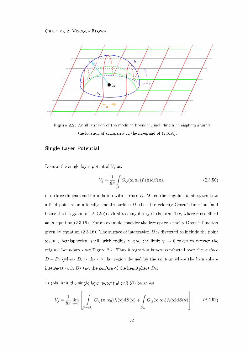
Figure 2.2: An illustration of the modied boundary including a hemisphere around
the location of singularity in the integrand of (2.3.50).
Single Layer Potential
Denote the single layer potential Vj as,
Vj =1
8π
∫D
Gij(x,x0)fi(x)dS(x), (2.3.50)
in a three-dimensional formulation with surface D. When the singular point x0 tends to
a eld point x on a locally smooth surface D, then the velocity Green's function (and
hence the integrand of (2.3.50)) exhibits a singularity of the form 1/r, where r is dened
as in equation (2.3.19). For an example consider the free-space velocity Green's function
given by equation (2.3.16). The surface of integration D is distorted to include the point
x0 in a hemispherical shell, with radius γ, and the limit γ → 0 taken to recover the
original boundary - see Figure 2.2. Thus integration is now conducted over the surface
D − Dc (where Dc is the circular region dened by the contour where the hemisphere
intersects with D) and the surface of the hemisphere Dh.
In this limit the single layer potential (2.3.50) becomes
Vj =1
8πlimγ→0
∫D−Dc
Gij(x,x0)fi(x)dS(x) +∫Dh
Gij(x,x0)fi(x)dS(x)
. (2.3.51)
32

Chapter 2: Viscous Flows
The rst integral in (2.3.51) tends to the original integral (2.3.50) in the limit dened.
The second integral of (2.3.51) can be rewritten as,
limγ→0
∫Dh
Gij(x,x0)fi(x)dS(x) = limγ→0
π2∫
0
2π∫0
Gij(x,x0)fi(x)γ2 sinφ dθdφ, (2.3.52)
where
Gij(x,x0) ∼ 1γ. (2.3.53)
Provided fi(x) is non-singular over the entire boundary, the integral in (2.3.52) can be
shown to tend to zero. Expression (2.3.51) becomes identical to (2.3.50) as x0 tends to
the surface, and the single-layer potential shows no discontinuity as x0 is moved onto
the boundary D. This result holds even for x0 placed at a corner of the boundary D,
although the analysis requires the hemisphere to be replaced by a portion of a sphere
dependent on the solid angle prescribed by the boundary shape at the corner.
Double Layer Potential
Consider the double-layer potential Wj from (2.3.49), with x0 interior to the domain,
Wj = − 18π
(i)∫D
ui(x)Tijk(x,x0)nk(x)dS(x), (2.3.54)
which can be rewritten as
Wj = − 18π
(i)∫D
[ui(x)− ui(x0)]Tijk(x,x0)nk(x)dS(x)
− 18πui(x0)
(i)∫D
Tijk(x,x0)nk(x)dS(x),
(2.3.55)
and note that the integrand of the rst integral in (2.3.55) is no longer singular (i.e.
the singularity of Tijk(x,x0)nk(x) is countered by its preceding term tending to zero).
Manipulating (2.3.55) and applying (2.3.33) (due to taking the singularity point initially
33
Chapter 2: Viscous Flows
within Vc and then moving to the boundary), allows expression (2.3.56) for the double-
layer potential to be derived when x0 lies directly on the locally smooth boundary D of
control volume Vc,
Wj = − 18π
x0∈D∫D
[ui(x)− ui(x0)]Tijk(x,x0)nk(x)dS(x)
− 18πui(x0)
x0∈D∫D
Tijk(x,x0)nk(x)dS(x) +12δijui(x0).
(2.3.56)
Rewriting (2.3.56) in the more convenient form using the standard properties of the
Kronecker delta yields
Wj = − 18π
x0∈D∫D
ui(x)Tijk(x,x0)nk(x)dS(x)
+1
8π
x0∈D∫D
ui(x0)Tijk(x,x0)nk(x)dS(x)
+12uj(x0)− 1
8π
x0∈D∫D
ui(x0)Tijk(x,x0)nk(x)dS(x),
(2.3.57)
and with x0 located on the boundary D, the middle and last integrals in (2.3.57) cancel
and the following important equation is obtained,
limx0→D
− 18π
(i)∫D
ui(x)Tijk(x,x0)nk(x)dS(x)
=
12uj(x0)− 1
8π
x0∈D∫D
ui(x)Tijk(x,x0)nk(x)dS(x).
(2.3.58)
The double-layer potential exhibits a discontinuity as the point x0 is moved onto the
boundary. The corresponding equation to (2.3.58) for the case of the singularity point
being located at a corner on the boundary D can be derived by similar means to those
shown. Using (2.3.36) in place of (2.3.33) in the above manipulation and following all
34

Chapter 2: Viscous Flows
the steps shown gives,
limx0→D
− 18π
(i)∫D
ui(x)Tijk(x,x0)nk(x)dS(x)
=
(1− Ω
4π
)uj(x0)− 1
8π
x0∈D∫D
ui(x)Tijk(x,x0)nk(x)dS(x)
(2.3.59)
The case of Ω = 2π corresponds to x0 placed on a locally smooth boundary and equation
(2.3.59) reduces to (2.3.58)
Direct Boundary Integral Equations
A general form for the BIE is found by (2.3.49), and using the continuous and discontin-
uous properties of the single and double layer potentials as x0 approaches the surface,
cij(x0)ui(x0) =1
8π
∫D
Gij(x,x0)fi(x)dS(x)
− 18π
∫D
ui(x)Tijk(x,x0)nk(x)dS(x),(2.3.60)
where cij(x0) denes the jump condition and is given by
cij(x0) =
δij when x0 is inside D,
12δij when x0 is on D,
0 when x0 is outside D,
(2.3.61)
for a smooth surface, and
cij(x0) =
δij when x0 is inside D,
Ω4π δij when x0 is on D,
0 when x0 is outside D,
(2.3.62)
at a corner point. Again, the case of Ω = 2π corresponds to x0 placed on a locally
smooth boundary and (2.3.62) reduces to (2.3.61).
The BIE (2.3.60) relates the governing boundary velocities and tractions for a Stokes ow.
Solutions of the BIE require boundary conditions suitable for the ow being analyzed.
35

Chapter 2: Viscous Flows
Three general possibilities of boundary conditions are described briey below. For more
details see [34, 37].
(i) If the boundary velocity u is specied over D, then the BIE becomes an equation
for the surface traction f only. This is called a Fredholm integral equation of the
rst kind.
(ii) If the surface traction f is specied over D, then the BIE becomes an equation for
the boundary velocity u only. This is called a Fredholm integral equation of the
second kind.
(iii) A Fredholm integral equation of mixed type involves specifying the boundary velocity
u over a part of D and for the remainder of D specifying the surface traction f .
Each of the resulting BIE is then solved for the unknown values on each section of
the boundary.
2.4 The Boundary Element Method
The boundary integral equation (BIE) for a singularity x0, located on a smooth bound-
ary D was derived in § 2.3 and is given by equation (2.3.60). The boundary element
method (BEM) is used as a means to solving the BIE on the boundary by implement-
ing three approximations. For suitable boundary conditions, the boundary elements are
collocated, resulting in a matrix problem to be solved for unknown boundary tractions
fi or velocities ui. These approximations along with the collocation of the boundary el-
ements are discussed in this section. Finally an example BEM implementation utilizing
a constant boundary distribution is described.
36
Chapter 2: Viscous Flows
2.4.1 Approximation And Collocation
The aim of the BEM is to reduce the BIE (2.3.60) to a matrix problem which can be
solved. To do this, three approximations are implemented. First of all the boundary is
discretized into elements by means of a geometrical approximation. Then the physical
variables are approximated on each of the previously dened elements by a chosen bound-
ary distribution. Finally, using an integral approximation, the integrals over each element
are evaluated using an appropriate numerical technique. Finally the resulting equation
can be collocated over all boundary elements to produce a system of equations that can
be solved. Each of these three approximations along with the collocation technique are
discussed in turn below.
Geometric Approximation
The boundary D of domain Vc over which the integrals of (2.3.60) are to be evaluated
often have complex geometries. It is appropriate to discretize the boundary D into
geometrically simpler boundary elements, denoted by Eν , ν = 1, . . . , N . The integrals in
(2.3.60) can then be rewritten as the sum of the integrals over each boundary elements
as shown in (2.4.1).
12uj(x0) =
18π
N∑ν=1
∫Eν
Gij(x,x0)fi(x)dS(x)
− 18π
N∑ν=1
∫Eν
ui(x)Tijk(x,x0)nk(x)dS(x).
(2.4.1)
Various forms of boundary discretization may be implemented, with the most common
cases comprising of either linear or quadratic triangular elements.
37
Chapter 2: Viscous Flows
Boundary Distribution
Values are required for the boundary traction fi and velocity ui on each of the bound-
ary elements Eν . The simplest approximation is to take the boundary tractions and
velocities constant over each element. However to improve accuracy, a variety of higher-
ordered polynomials, or other kinds of interpolation function can be used to represent
the boundary distributions.
Integral Approximation
The integrals in equation (2.4.1) need evaluating on each element that discretizes the
boundary. These integrals can be classied as,
• Non-Singular : The element over which the integration is to be conducted does not
contain the singularity x0 and the integrands are non-singular in this case.
• Singular : The element over which the integration is to be conducted contains the
singularity x0 and the integrands are singular in this case.
In general the integrals will be evaluated using a range of numerical methods for both
non-singular and singular integrands. Non-singular integrands are evaluated numerically
using appropriate Gaussian quadrature techniques. For cases of near-point singularities,
renement of the integration is made by a combination of an adaptive Gaussian integra-
tion algorithm and an element subdivision approach. Further details of this method are
given in chapter 4. Singularities of the single layer potential are evaluated using polar
integration, with details omitted here but shown in [34]. Flat elements are considered
throughout this thesis, causing the singularity of the double layer potential to vanish
due to the tangent vector of a at element always being perpendicular to the normal.
38

Chapter 2: Viscous Flows
Collocation Of Boundary Elements
When suitable boundary conditions are applied, which dene either the boundary trac-
tion fi or velocity ui on each element, then it is left for the BEM to calculate the unknown
values of fi or ui on each element. This is achieved by collocation of the discretized equa-
tion in a bid to generate the same number of equations as unknowns. A matrix problem
is formulated and solved for the unknown values associated with the Stokes ow.
2.4.2 Implementation Of A Constant Boundary Distribution
This section considers the BEM formulation outlined above for a constant boundary dis-
tribution. Details of the geometrical approximation and the type of numerical techniques
used for the evaluation of the integrals are not required per se as they will have no eect
on the formulation shown below.
Consider a geometric approximation, used to discretize the boundary into N elements.
As described in the previous section, the integral (2.3.60) is simplied to the sum of
the integrals over each element, as shown in (2.4.1). In addition a constant or uniform
boundary distribution implies a constant value for boundary traction fi and velocity ui
be dened over each element. These are written as fi|Eν and ui|Eν for element Eν . Also
note that from here on dS ≡ dS(x). Substituting these values into equation (2.4.1)
yields,
12uj(x0) =
18π
N∑ν=1
fi|Eν∫Eν
Gij(x,x0)dS
− 18π
N∑ν=1
ui|Eν∫Eν
Tijk(x,x0)nk(x)dS.
(2.4.2)
Equation (2.4.2) can be rewritten such that the summation used for the evaluation of
39
Chapter 2: Viscous Flows
uj(x0) is via the multiplication of vectors,
12uj(x0) =
18π
(fi|Eν=1 , · · · , fi|Eν=N
)∫Eν=1Gij(x,x0)dS
...∫Eν=N Gij(x,x0)dS
− 18π
(ui|Eν=1 , · · · , ui|Eν=N
)∫Eν=1 Tijk(x,x0)nkdS
...∫Eν=N Tijk(x,x0)nkdS
.
(2.4.3)
By placing the singularity point x0 at the middle of element ζ, denoted xMζ and recalling
the values of fi and ui are taken constant over each element, the left hand side of (2.4.3)
becomes,
12uj(xMζ ) =
12uj |Eζ . (2.4.4)
By collocating over all the elements, (2.4.2) becomes a system of 3N equations comprising
of the 3 components of ui, fi on each of the N elements. Two 3N × 3N matrices are
formed, which can be thought of as N × N arrays where each component is the 3 × 3
matrix Gij or Tijknk (where i is the local row number and j is the local column number
of each component within the N × N array). Thus the collocated system of equations
determined by the BEM is given by.
12Ud =
18πFcAcd −
18πUcBcd, (2.4.5)
where
Fc =(fi|Eν=1 · · · fi|Eν=N
), (2.4.6)
Uc =(ui|Eν=1 · · · ui|Eν=N
), (2.4.7)
Acd =
∫Eν=1Gij(x,x
Mζ=1)dS · · ·
∫Eν=1Gij(x,x
Mζ=N )dS
.... . .
...∫Eν=N Gij(x,x
Mζ=1)dS · · ·
∫Eν=N Gij(x,x
Mζ=N )dS
, (2.4.8)
Bcd =
∫Eν=1 Tijk(x,x
Mζ=1)nkdS · · ·
∫Eν=1 Tijk(x,x
Mζ=N )nkdS
.... . .
...∫Eν=N Tijk(x,x
Mζ=1)nkdS · · ·
∫Eν=N Tijk(x,x
Mζ=N )nkdS
, (2.4.9)
40

Chapter 2: Viscous Flows
for i, j, k = 1, . . . , 3, and ν, ζ = 1, . . . , N . Indices c and d take values c, d = 1, . . . , 3N
and are dened by.
c = 3(ν − 1) + i, (2.4.10)
d = 3(ζ − 1) + j. (2.4.11)
Rewritten (2.4.5) becomes
18πFcAcd = Uc
(12δcd +
18πBcd
). (2.4.12)
The solution of (2.4.12) involves calculating the integrals of each element, and forming
the components of the two matrices. By specifying suitable boundary conditions the
system of equations is solved for unknown tractions and/or velocities.
41

Chapter 3
Radial Basis Functions
Solutions of lm ows down an inclined plane over and around obstacles require a range
of ecient numerical techniques. These lm proles are often dominated by surface forces
such as surface tension, and require an accurate representation of the free surface. The
evaluation of the free surface traction, incorporating these eects, is achieved by using a
radial basis function (RBF). In addition by using a Hermitian RBF, far eld and contact
line constraints imposed on the free surface can also be included in the interpolation. A
RBF interpolation is also used in Chapter 7 when implementing numerical techniques to
extend a Stokes ow formulation to the non-linear problem of nite Reynolds number
ows. This chapter considers an overview of RBFs, along with implementation of local
and global interpolations.
3.1 Introduction To Radial Basis Function Interpolations
The interpolation of a discrete set of data points, such as those obtained by mesh based
schemes, (e.g. the boundary element method (BEM)), is a common problem. Conven-
tional methods such as polynomial and spline interpolations have been applied to a wide
range of engineering problems. Alternatively a radial basis function (RBF) interpolation
can be used for such a purpose. An extensive study of interpolation methods available
at the time was conducted by Franke [40], and concluded that RBF interpolations were
42

Chapter 3: Radial Basis Functions
Generalized Thin Plate Spline (2D) r2m−2 log r
Generalized Thin Plate Spline (3D) rm (m odd)
Generalized Multiquadric(r2 + c2
)m2 (m odd)
Gaussian exp(− rc
)Table 3.1: Common radial basis functions
the most accurate techniques evaluated.
The theory of RBFs originated as a means to provide a continuous interpolation of scat-
tered data values. However, in recent years RBFs have been extensively researched and
applied in a wider range of analysis. Partial dierential equations (PDEs) have been
solved using RBFs with recent work in this eld conducted by La Rocca et al. [41] and
La Rocca and Power [42]. The RBF interpolation has also been used in the implemen-
tation of the dual reciprocity method (DRM) (see Nardini and Brebbia [43]), a method
used to transform the domain integrals present in the boundary integral equations (BIEs)
for non-linear problems. In this thesis the original application of RBFs is used as a means
of interpolating the surface data for lm ow over or around an obstacle. In addition,
chapter 7 considers the non-linear problem of lm ows at nite Reynolds number, using
a RBF interpolation within the numerical techniques implemented.
A RBF ψ(‖x − ξj‖) depends on the separation between a eld point x and the data
centres ξj , for j = 1, . . . , N , and N data points. The interpolants are classed as radial
due to their spherical symmetry around centres ξj , with ‖x − ξj‖ the Euclidean norm.
The most popular RBFs are listed in table 3.1 where r = ‖x− ξj‖, m is an integer, and
c is a free parameter, often referred to as the shape parameter, to be specied by the
user. In addition, for the multiquadric and the three-dimensional thin plate spline, only
odd values of m are permitted.
The inverse multiquadric (m < 0 in the generalized multiquadric) and Gaussian are
functions which form positive denite interpolation matrices, whilst the thin plate spline
43
Chapter 3: Radial Basis Functions
and multiquadric (m > 0 in the generalized multiquadric) are functions which generate
conditionally positive denite matrices of order m. By standard theory, positive de-
nite matrices are never singular, and guarantee solution to the interpolation problem.
However, the conditionally positive denite matrices which are formed by RBFs such as
the thin plate spline may be singular for certain selections of data centres. These condi-
tionally positive denite matrices are conditionate of a polynomial of order m− 1 along
with homogeneous constraint condition. If these are included within the interpolation,
a positive denite matrix is formed, and solution to the interpolation is guaranteed. For
further details, see Golberg and Chen [44].
The shape parameter c within the Gaussian and multiquadric RBFs requires ne tuning
and can dramatically alter the quality of the interpolation. Despite being considered
as optimal for interpolating multivariate data, Franke [40] found that the thin plate
spline was marginally outperformed by the multiquadric RBF with regards to the test
criteria. In fact Powell [45] indicated that the thin plate spline RBF only converges
linearly compared to the multiquadrics which converge exponentially, producing a min-
imal semi-norm error (see Madych and Nelson [46]). However, the multiquadric RBF
is disadvantaged by the presence of the shape parameter c whose choice signicantly
eects the interpolation. In addition, Schaback [47] states that numerical experiments
show that the condition number of the resulting interpolation matrix is large for smooth
interpolants such as the gaussian or multiquadric RBF when compared to non-smooth
functions such as thin plate splines for low m. Thus a thin plate spline RBF is used
throughout this thesis.
Typical interpolation problems involve taking the known data centres(ξj , F (ξj)
), for
j = 1, . . . , N of the unknown function F and interpolating it by the function f . Thus
for a conditionally positive denite function, the interpolation takes the form,
f(x) =N∑j=1
λjψ(‖x− ξj‖
)+ Pm−1(x), (3.1.1)
and for arbitrary orderm, the polynomial Pm−1 containsNp terms and in two-dimensions
44
Chapter 3: Radial Basis Functions
has the expanded form
Pm−1(xi) = λN+1(xi1)m−1+λN+2(xi2)m−1 + λN+3(xi1)m−2xi2 + . . .
+ λN+Np−2xi1 + λN+Np−1x
i2 + λN+Np .
(3.1.2)
Collocation of (3.1.1) over the N data centres yields N equations for the N + Np un-
knowns λj . The homogeneous constraint condition,
N∑j=1
λjPk(xj) = 0, 1 ≤ k ≤ m− 1, (3.1.3)
gives another Np equations to close the system. Thus, by collocation over the data
centres, a matrix problem Aijλj = bi is formed, where Aij is dened by,
Aij =
ψ Pm−1
(Pm−1)T 0
, (3.1.4)
and bi is given by,
bi =
(F 0
)T. (3.1.5)
The matrix problem can be solved for λj , and thus the function f(x) can be reconstructed
at any point by (3.1.1).
Hermitian Interpolations And Double Collocation
When the problem species additional constraints (for example far eld conditions), they
can be incorporated by use of a Hermite RBF interpolation. Consider the linear partial
dierential operator Lx(f(x)) = G to be applied at n points which may or may not
correspond to locations used in the original interpolation (3.1.1). Then the Hermitian
interpolation takes the form
f(x) =N∑j=1
λjψ(‖x− ξj‖
)+
N+n∑j=N+1
λjLξψ(‖x− ξj‖
)+ Pm−1(x), (3.1.6)
where Lξ is the dierential operator dened above but acting on ξ.
45

Chapter 3: Radial Basis Functions
For the Hermite interpolation (3.1.6), a matrix problem Aijλj = bi is formed, where Aij
is now dened by,
Aij =
ψ Lξ(ψ) Pm−1
Lx(ψ) LxLξ(ψ) Lx(Pm−1)
(Pm−1)T (Lx(Pm−1))T 0
, (3.1.7)
and bi is given by,
bi =
(F G 0
)T. (3.1.8)
The matrix (3.1.7) is non-singular as long as ψ is chosen appropriately. For cases of
double collocation, ψ, Lx(ψ) and any further dierential operators can be applied simul-
taneously at the same collocation points as long as they are linearly independent.
When modelling lm ow over an obstacle, an accurate method for generating the free
surface and deducing the unit normal and curvature is required. By supplying a discrete
set of data points (surface heights), a Hermitian RBF can be used to nd a smooth
function through all of the points, allowing the derivative of the free surface and hence
the unit normal and mean curvature to be found.
3.2 Local And Global Interpolations
The radial basis function (RBF) interpolation outlined in section 3.1 is described in a
global sense. The interpolation matrix involves solving a system of equations that incor-
porate all data points. For anN×N interpolation matrix, this requires O(N3) operations
when using Gaussian elimination to solve the system of equations. For large systems the
amount of CPU time and RAM necessary can become prohibitive. In addition, as the
system becomes large, the resulting matrix becomes ill-conditioned. The local RBF can
oer substantial improvements with regards to the CPU time and RAM requirements,
46
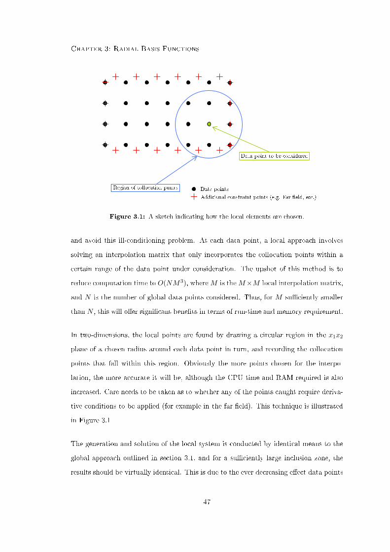
Chapter 3: Radial Basis Functions
Figure 3.1: A sketch indicating how the local elements are chosen.
and avoid this ill-conditioning problem. At each data point, a local approach involves
solving an interpolation matrix that only incorporates the collocation points within a
certain range of the data point under consideration. The upshot of this method is to
reduce computation time to O(NM3), whereM is theM×M local interpolation matrix,
and N is the number of global data points considered. Thus, for M suciently smaller
than N , this will oer signicant benets in terms of run-time and memory requirement.
In two-dimensions, the local points are found by drawing a circular region in the x1x2
plane of a chosen radius around each data point in turn, and recording the collocation
points that fall within this region. Obviously the more points chosen for the interpo-
lation, the more accurate it will be, although the CPU time and RAM required is also
increased. Care needs to be taken as to whether any of the points caught require deriva-
tive conditions to be applied (for example in the far eld). This technique is illustrated
in Figure 3.1
The generation and solution of the local system is conducted by identical means to the
global approach outlined in section 3.1, and for a suciently large inclusion zone, the
results should be virtually identical. This is due to the ever decreasing eect data points
47

Chapter 3: Radial Basis Functions
will have on the interpolation further away from the point under consideration. The
eciency gains from using a local interpolation will be evaluated for each case imple-
mented. In general when interpolating the free surface, a global technique is optimum.
However, when considering the eects of inertia using the method of particular solutions
in chapter 7, a local approach is often benecial.
48
Chapter 4
Stokes Flow Over A Single Obstacle
Thin lm ows driven by gravity down an inclined plane and over an obstacle is an
important, well studied generic ow problem. Ecient and accurate solution techniques
are developed in this chapter based on a Stokes ow formulation. In § 1.1 a thorough
overview of published works in this eld are considered, with this chapter starting by
considering the formulation and numerical schemes to be used in solving the problem,
outlined in § 4.1 and § 4.2 respectively. Finally, solutions for Stokes ow over a single
obstacle are considered in § 4.3, validating results with those previously published by
other authors.
4.1 Mathematical Formulation
This section considers the Stokes ow formulation of a thin lm driven by gravity down
an inclined plane over an obstacle attached to the plane. The ow variables are solved
for disturbance and undisturbed components in a manner similar to Blyth and Pozrikidis
[31]. Two subsections outline the simplication of the formulation for consideration of
small free surface deections as in [31] and consideration of asymptotically small obstacles
as implemented by Pozrikidis and Thoroddsen [29].
A two-dimensional schematic of a typical lm ow of undisturbed thickness H, driven
49
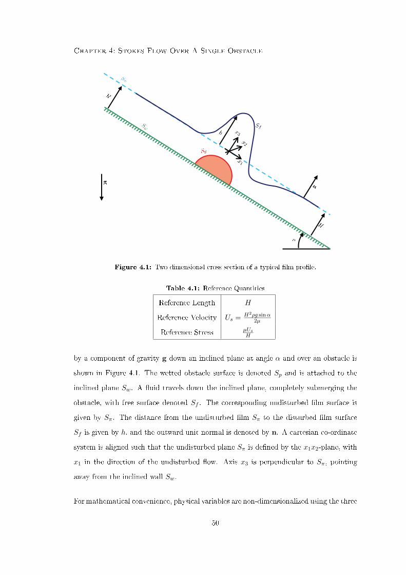
Chapter 4: Stokes Flow Over A Single Obstacle
Figure 4.1: Two-dimensional cross section of a typical lm prole.
Table 4.1: Reference Quantities
Reference Length H
Reference Velocity Us = H2ρg sinα2µ
Reference Stress µUsH
by a component of gravity g down an inclined plane at angle α and over an obstacle is
shown in Figure 4.1. The wetted obstacle surface is denoted Sp and is attached to the
inclined plane Sw. A uid travels down the inclined plane, completely submerging the
obstacle, with free surface denoted Sf . The corresponding undisturbed lm surface is
given by Sπ. The distance from the undisturbed lm Sπ to the disturbed lm surface
Sf is given by h, and the outward unit normal is denoted by n. A cartesian co-ordinate
system is aligned such that the undisturbed plane Sπ is dened by the x1x2-plane, with
x1 in the direction of the undisturbed ow. Axis x3 is perpendicular to Sπ, pointing
away from the inclined wall Sw.
For mathematical convenience, physical variables are non-dimensionalized using the three
50
Chapter 4: Stokes Flow Over A Single Obstacle
reference quantities shown in table 4.1. The reference length is taken as the undisturbed
lm height H, with reference velocity given by the free stream surface velocity Us for
lm ow down an inclined plane in the absence of an obstacle. Finally, a viscous scaling
is used for the reference stress. The associated Bond number is
Bo =ρgH2 sinα
γ, (4.1.1)
where γ is the surface tension, ρ the uid density and g = |g| the acceleration due to
gravity.
The lm ow is governed by the standard incompressible equations for mass conservation
(4.1.2) and steady Stokes ow (4.1.3)
∂ui∂xi
= 0, (4.1.2)
− ∂p
∂xi+∂G
∂xi+∂2ui∂x2
j
= 0, (4.1.3)
where G is dened by (4.1.4),
G = −2(x3 cotα− x1). (4.1.4)
Far eld constraints involve the ow velocity and pressure returning to values associated
with a gravity driven lm ow down an inclined plane in the absence of an obstacle,
and denoted by a superscript ∞. In addition, the free surface deection, along with the
gradient of the free surface should decay to zero. These conditions are shown in (4.1.5),
ui → u∞i
p→ p∞
h→ 0
∂h∂x1→ 0
∂h∂x2→ 0
as x→ ±∞. (4.1.5)
Several boundary conditions are also applied within the ow domain. No slip (zero
velocity) is specied on the inclined wall Sw, and wetted obstacle surface Sp, given by
51
Chapter 4: Stokes Flow Over A Single Obstacle
(4.1.6). In addition a dynamic (4.1.7) and kinematic (4.1.8) condition are applied on the
free surface Sf , and expressed as,
ui = 0 x ∈ Sw ∪ Sp, (4.1.6)
fi = σijnj = − 4Bo
κni x ∈ Sf , (4.1.7)
∂h
∂t= −u1
∂h
∂x1− u2
∂h
∂x2+ u3 x ∈ Sf , (4.1.8)
where fi is the boundary traction. The curvature of the free surface is denoted by κ,
σij is the stress tensor, and time is given by t. The curvature and the stress tensor are
expressed by (4.1.9) and (4.1.10):
κ =12∂ni∂xi
, (4.1.9)
σij = −pδij +(∂ui∂xj
+∂uj∂xi
). (4.1.10)
In (4.1.9) and (4.1.10) ni is the components of the outward unit normal to the free surface
Sf . The outward unit normal ni of the free surface can be evaluated as,
n =1√
1 +(∂h∂x1
)2+(∂h∂x2
)2
(− ∂h
∂x1,− ∂h
∂x2, 1). (4.1.11)
The form of the curvature κ can also be expanded as,
κ =− 12
(1 +
(∂h
∂x1
)2
+(∂h
∂x2
)2)− 3
2
×[∂2h
∂x21
(1 +
(∂h
∂x2
)2)
+∂2h
∂x22
(1 +
(∂h
∂x1
)2)− 2
∂2h
∂x1∂x2
∂h
∂x1
∂h
∂x2
].
(4.1.12)
Film Flow In The Absence Of Obstacles
The governing equations for lm ow in the absence of obstacles, is given by
∂u∞i∂xi
= 0, (4.1.13)
−∂p∞
∂xi+∂G
∂xi+∂2u∞i∂x2
j
= 0, (4.1.14)
52
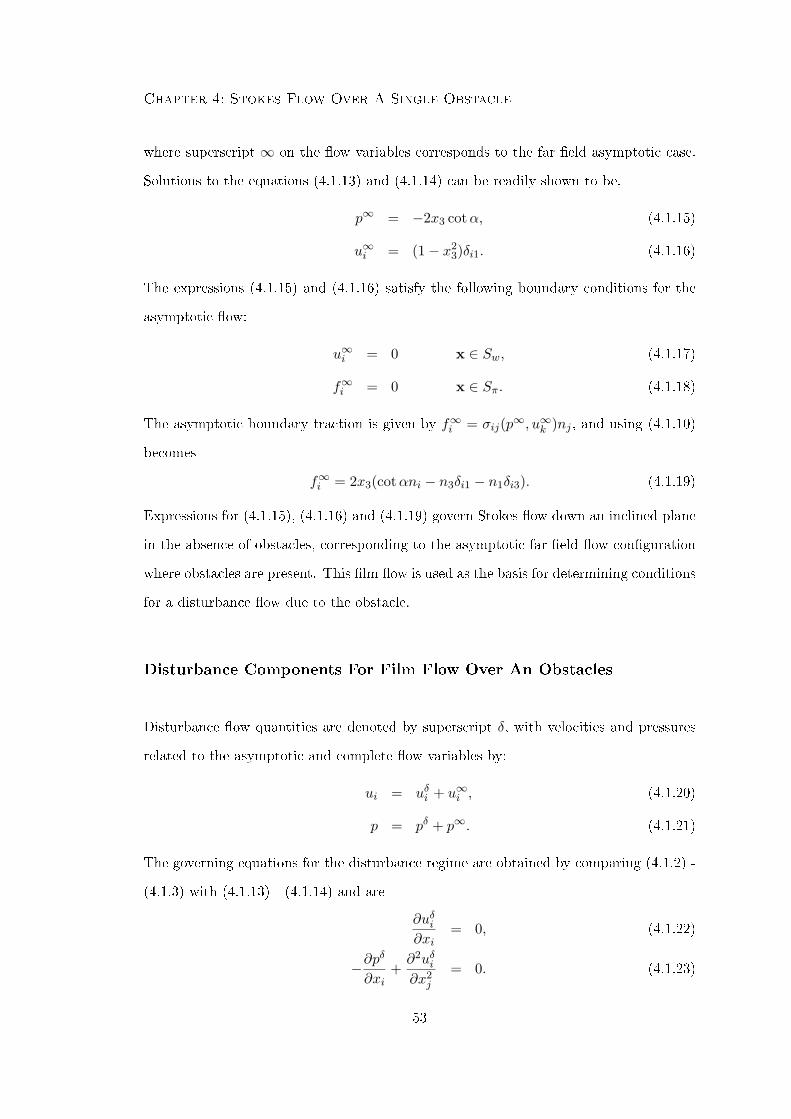
Chapter 4: Stokes Flow Over A Single Obstacle
where superscript ∞ on the ow variables corresponds to the far eld asymptotic case.
Solutions to the equations (4.1.13) and (4.1.14) can be readily shown to be,
p∞ = −2x3 cotα, (4.1.15)
u∞i = (1− x23)δi1. (4.1.16)
The expressions (4.1.15) and (4.1.16) satisfy the following boundary conditions for the
asymptotic ow:
u∞i = 0 x ∈ Sw, (4.1.17)
f∞i = 0 x ∈ Sπ. (4.1.18)
The asymptotic boundary traction is given by f∞i = σij(p∞, u∞k )nj , and using (4.1.10)
becomes
f∞i = 2x3(cotαni − n3δi1 − n1δi3). (4.1.19)
Expressions for (4.1.15), (4.1.16) and (4.1.19) govern Stokes ow down an inclined plane
in the absence of obstacles, corresponding to the asymptotic far eld ow conguration
where obstacles are present. This lm ow is used as the basis for determining conditions
for a disturbance ow due to the obstacle.
Disturbance Components For Film Flow Over An Obstacles
Disturbance ow quantities are denoted by superscript δ, with velocities and pressures
related to the asymptotic and complete ow variables by:
ui = uδi + u∞i , (4.1.20)
p = pδ + p∞. (4.1.21)
The governing equations for the disturbance regime are obtained by comparing (4.1.2) -
(4.1.3) with (4.1.13) - (4.1.14) and are
∂uδi∂xi
= 0, (4.1.22)
−∂pδ
∂xi+∂2uδi∂x2
j
= 0. (4.1.23)
53

Chapter 4: Stokes Flow Over A Single Obstacle
Far eld conditions for the disturbance regime require the variables to decay to zero, and
ow velocity and pressure to return to the values associated with the asymptotic regime,
as seen in (4.1.5). Thus uδi and pδ are subject to the following conditions in the far eld:
uδi → 0
pδ → 0
as x→ ±∞. (4.1.24)
No-slip boundary conditions for the disturbance velocity uδi can also be specied on
the wall Sw and wetted obstacle boundary Sp by comparing (4.1.6) with (4.1.17) and
requires:
uδi = 0 x ∈ Sw, (4.1.25)
uδi = −u∞i x ∈ Sp. (4.1.26)
Finally an expression for the boundary traction associated with the disturbance ow f δi
can be dened on the free surface Sf by comparing (4.1.7) and (4.1.19). The expression
for f δi is
f δi = − 4Bo
κni − 2x3(cotαni − n3δi1 − n1δi3), (4.1.27)
where κ is the curvature associated with the disturbed free surface.
Boundary Integral Formulation For Flow Over An Obstacle
For the disturbance regime, the governing equations for Stokes ow (4.1.22) - (4.1.23)
can be expressed exactly as a boundary integral equation (BIE) over the uid domain
(4.1.28)
cij(x0)uδi (x0) =1
8π
∫Sf∪Sp
G∗ij(x,x0)f δi (x)dS(x)
− 18π
∫Sf∪Sp
uδi (x)T ∗ijk(x,x0)nk(x)dS(x),(4.1.28)
where x is the eld point within the analysis, and x0 any collocation point. The Green's
functions G∗ij(x,x0), T ∗ijk(x,x0) in (4.1.28) are the Lorentz-Blake Green's function for
54
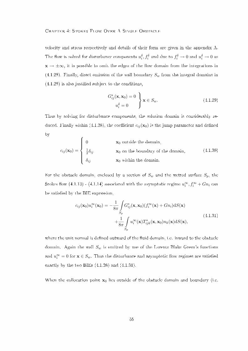
Chapter 4: Stokes Flow Over A Single Obstacle
velocity and stress respectively and details of their form are given in the appendix A.
The ow is solved for disturbance components uδi , fδi and due to f δi → 0 and uδi → 0 as
x → ±∞, it is possible to omit the edges of the ow domain from the integrations in
(4.1.28). Finally, direct omission of the wall boundary Sw from the integral domains in
(4.1.28) is also justied subject to the conditions,
G∗ij(x,x0) = 0
uδi = 0
x ∈ Sw. (4.1.29)
Thus by solving for disturbance components, the solution domain is considerably re-
duced. Finally within (4.1.28), the coecient cij(x0) is the jump parameter and dened
by
cij(x0) =
0 x0 outside the domain,
12δij x0 on the boundary of the domain,
δij x0 within the domain.
(4.1.30)
For the obstacle domain, enclosed by a section of Sw and the wetted surface Sp, the
Stokes ow (4.1.13) - (4.1.14) associated with the asymptotic regime u∞i , f∞i +Gni can
be satised by the BIE expression,
cij(x0)u∞i (x0) = − 18π
∫Sp
G∗ij(x,x0)(f∞i (x) +Gni)dS(x)
+1
8π
∫Sp
u∞i (x)T ∗ijk(x,x0)nk(x)dS(x),(4.1.31)
where the unit normal is dened outward of the uid domain, i.e. inward to the obstacle
domain. Again the wall Sw is omitted by use of the Lorentz-Blake Green's functions
and u∞i = 0 for x ∈ Sw. Thus the disturbance and asymptotic ow regimes are satised
exactly by the two BIEs (4.1.28) and (4.1.31).
When the collocation point x0 lies outside of the obstacle domain and boundary (i.e.
55

Chapter 4: Stokes Flow Over A Single Obstacle
x0 /∈ Sp,Ωp ), (4.1.31) and (4.1.30) gives,
18π
∫Sp
G∗ij(x,x0)(f∞i (x) +Gni)dS(x)
=1
8π
∫Sp
u∞i (x)T ∗ijk(x,x0)nk(x)dS(x).(4.1.32)
The BIE (4.1.28) associated with the disturbance regime can be modied by taking
collocation on the free surface (x0 ∈ Sf ), and applying (4.1.26), yielding
12uδj(x0) =
18π
∫Sf
G∗ij(x,x0)f δi (x)dS(x)
− 18π
∫Sf
uδi (x)T ∗ijk(x,x0)nk(x)dS(x)
18π
∫Sp
G∗ij(x,x0)f δi (x)dS(x)
+1
8π
∫Sp
u∞i (x)T ∗ijk(x,x0)nk(x)dS(x).
(4.1.33)
Combining (4.1.32) and (4.1.33) gives a BIE with collocation over the free surface:
12uδj(x0) +
18π
∫Sf
uδi (x)T ∗ijk(x,x0)nk(x)dS(x)
=1
8π
∫Sp
G∗ij(x,x0)fi(x)dS(x)
+1
8π
∫Sf
G∗ij(x,x0)f δi (x)dS(x) x0 ∈ Sf ,
(4.1.34)
where fi(x) = fi(x) +Gni.
Collocating the BIE for the asymptotic regime (4.1.31) at the wetted obstacle surface
x0 ∈ Sp yields,
12u∞j (x0) = − 1
8π
∫Sp
G∗ij(x,x0)f∞i (x)dS(x)
+1
8π
∫Sp
u∞i (x)T ∗ijk(x,x0)nk(x)dS(x),(4.1.35)
56

Chapter 4: Stokes Flow Over A Single Obstacle
where f∞i (x) = f∞i (x) +Gni. The disturbance BIE (4.1.28) can be collocated over the
wetted obstacle surface x0 ∈ Sp, with the no slip condition (4.1.26) to form,
−12u∞j (x0) =
18π
∫Sf
G∗ij(x,x0)f δi (x)dS(x)
− 18π
∫Sf
uδi (x)T ∗ijk(x,x0)nk(x)dS(x)
+1
8π
∫Sp
G∗ij(x,x0)f δi (x)dS(x)
+1
8π
∫Sp
u∞i (x)T ∗ijk(x,x0)nk(x)dS(x).
(4.1.36)
Combining (4.1.35) and (4.1.36) yields (4.1.37), a BIE for collocation over the wetted
obstacle surface Sp:
18π
∫Sp
G∗ij(x,x0)fi(x)dS(x)
= −u∞j (x0)− 18π
∫Sf
G∗ij(x,x0)f δi (x)dS(x)
+1
8π
∫Sf
uδi (x)T ∗ijk(x,x0)nk(x)dS(x) x0 ∈ Sp.
(4.1.37)
In summary the steady, gravity driven Stokes ow down an inclined plane over an obstacle
is governed exactly by solutions satisfying the BIEs (4.1.37) and (4.1.34). The ow
is subject to a kinematic condition (4.1.8), a dynamic condition (4.1.7), and far eld
constraints (4.1.5). Flow over a single obstacle are governed by, plane inclination angle
α, the obstacle geometry, and the Bond number Bo.
4.1.1 Small Free Surface Deections
Pozrikidis and Thoroddsen [29] and Blyth and Pozrikidis [31] simplied ow over a hemi-
sphere through the assumption of a small free surface deection. By assuming the free
surface disturbance remains small, when compared to the undisturbed lm thickness, and
57

Chapter 4: Stokes Flow Over A Single Obstacle
the disturbance velocities at the free surface are small when compared to the undisturbed
lm speed at the same point then
h 1, uδi 1, i = 1, 2, 3. (4.1.38)
Assuming asymptotically small disturbances, the unit normal on the free surface is ap-
proximated by
n = (0, 0, 1) +(− ∂h
∂x1,− ∂h
∂x2, 0), (4.1.39)
where the components in the x1x2-plane are considered small. Thus,
∂ni∂xi≈ −∂
2h
∂x21
− ∂2h
∂x22
≡ −∇2x1x2
h. (4.1.40)
The disturbance boundary traction (4.1.27) approximates to,
f δi = 2hδi1 +(
2Bo∇2x1x2
h− 2h cotα)δi3, (4.1.41)
at leading order. To the same order of approximation the kinematic condition (4.1.8)
becomes
∂h
∂t= − ∂h
∂x1+ uδi δi3. (4.1.42)
Finally the BIEs for ow over an obstacle,(4.1.34) and (4.1.37) simplify to integrals over
the undisturbed surface Sπ (x3 = 0) and become,
12uδj(x0)+
18π
∫Sπ
uδi (x)T ∗ijk(x,x0)nk(x)dS(x)
=1
8π
∫Sp
G∗ij(x,x0)fi(x)dS(x)
+1
8π
∫Sπ
G∗ij(x,x0)f δi (x)dS(x) x0 ∈ Sπ,
(4.1.43)
and
18π
∫Sp
G∗ij(x,x0)fi(x)dS(x)
= −u∞j (x0)− 18π
∫Sπ
G∗ij(x,x0)f δi (x)dS(x)
+1
8π
∫Sπ
uδi (x)T ∗ijk(x,x0)nk(x)dS(x) x0 ∈ Sp.
(4.1.44)
58

Chapter 4: Stokes Flow Over A Single Obstacle
Pozrikidis and Thoroddsen [29] and Blyth and Pozrikidis [31] consider this small de-
ection simplication in combination with nite dierence approximations (FDAs) for
evaluating all derivatives. However, this assumption is not relevant for nite free surface
deections as of interest here, with the small deection analysis used only for verication
with the previously published work.
4.1.2 Flow Over Asymptotically Small Obstacles
A further simplication to the boundary integral analysis can be made when the obstacle
is asymptotically small. Asymptotic analysis of the obstacle is conducted by following
Blyth and Pozrikidis [31] which reproduced the earlier work of Pozrikidis and Thoroddsen
[29]. A brief summary of the method is reproduced here, and the reader is referred to
[29, 31] for full details.
The aim of the asymptotic analysis is to produce an expression for the obstacle integral
Sp, in (4.1.43), eliminating the need for solving (4.1.44). This rst term of the right
hand side of (4.1.43) can be rewritten using the symmetry property (2.3.21) as,
18π
∫Sp
G∗ij(x,x0)fi(x)dS(x) =1
8π
∫Sp
G∗ji(x0,x)fi(x)dS(x). (4.1.45)
We consider a small spherical obstacle, with radius a and in contact with a plane wall
and assume that the obstacle is much smaller than the undisturbed, non-dimensionalized
lm height, a 1. Then it is possible to expand the velocity Green's function G∗ji using
a Taylor series with respect to d, where d = x3 − x3wall = x3 + 1 is the vertical distance
from the point x3 on the obstacle to the plane wall, and is illustrated in gure 4.2. The
Lorentz-Blake Green's function are shown in appendix A (where h0 is equivalent to d
here), with the order of the indices and arguments shown in reverse to (4.1.45). The
59

Chapter 4: Stokes Flow Over A Single Obstacle
Figure 4.2: Two-dimensional cross section indicating the asymptotic formulation of
the lm prole.
Taylor series is written as,
G∗ji(x0,x) ≈ G∗ji(x0,xp) + d∂
∂x3
(G∗ji(x0,x)
)∣∣∣∣x=xp
+d2
2∂2
∂x23
(G∗ji(x0,x)
)∣∣∣∣x=xp
+ . . . ,
(4.1.46)
where the non-dimensional point xp is dened as
xp = (0, 0,−1). (4.1.47)
The case of i = 3 requires separate consideration to i = 1, 2 with the Taylor series shown
to give to leading order,
G∗jm(x0,x) ≈ dMjm(X) m = 1, 2, (4.1.48)
G∗j3(x0,x) ≈ d2Mj3(X), (4.1.49)
60

Chapter 4: Stokes Flow Over A Single Obstacle
where
X = x0 − xp, (4.1.50)
Mjm(X) = 12XmXjX3
|X|5, m = 1, 2 (4.1.51)
Mj3(X) = −6X3
(2Xj
|X|5+δj3X3
|X|5− 5X2
3Xj
|X|7
). (4.1.52)
The integral (4.1.45) becomes
18π
∫Sp
G∗ji(x0,x)fi(x)dS(x) ≈ 18πMjm(X)
∫Sp
dfm(x)dS(x)
+1
8πMj3(X)
∫Sp
d2f3(x)dS(x) m = 1, 2.(4.1.53)
This is analogous to the work in [29] when the dierence in the denition of the co-
ordinate axis is taken into account.
From [29], the following scalings are introduced,∫Sp
dfm(x)dS(x) = −8πa3cm∂u∞x∂x3
∣∣∣∣x3=−1
, m = 1, 2 (4.1.54)
∫Sp
d2f3(x)dS(x) = −8πa4c3∂u∞x∂x3
∣∣∣∣x3=−1
, (4.1.55)
where the sign on the right hand side is generated from taking the outward unit normal
instead of inward as specied in [29] resulting in an opposite sign for the boundary
traction fi. In (4.1.54) - (4.1.55), the distance d is taken to scale like the radius a, and
the traction fi, scales like the shear stress∂u∞x∂x3
∣∣∣x3=−1
. Both of these are independent of
the integration, which as a result yields the surface area of a sphere 4πa2. For equality,
a constant vector 2c3 and 2cm, m = 1, 2 is required and depends on the geometry of the
obstacle. For the case of a spherical obstacle the terms of c are given by the work of
[29], which extracts them from O'Neill [48] and gives them to be,
c1 = −16
∞∫0
A(s)(
3− 8s coth s+ 7s2
sinh2 s− 2
s3
sinh2 scoth s
)ds, (4.1.56)
c2 = 0, (4.1.57)
c3 = 0, (4.1.58)
61
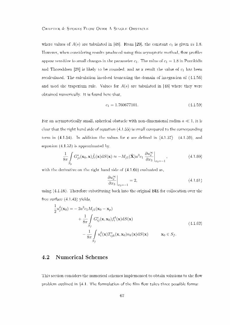
Chapter 4: Stokes Flow Over A Single Obstacle
where values of A(s) are tabulated in [48]. From [29], the constant c1 is given as 1.8.
However, when considering results produced using this asymptotic method, ow proles
appear sensitive to small changes in the parameter c1. The value of c1 = 1.8 in Pozrikidis
and Thoroddsen [29] is likely to be rounded, and as a result the value of c1 has been
recalculated. The calculation involved truncating the domain of integration of (4.1.56)
and used the trapezium rule. Values for A(s) are tabulated in [48] where they were
obtained numerically. It is found here that,
c1 = 1.760677101. (4.1.59)
For an asymptotically small, spherical obstacle with non-dimensional radius a 1, it is
clear that the right hand side of equation (4.1.55) is small compared to the corresponding
term in (4.1.54). In addition the values for c are dened in (4.1.57) - (4.1.59), and
equation (4.1.53) is approximated by,
18π
∫Sp
G∗ji(x0,x)fi(x)dS(x) ≈ −Mj1(X)a3c1∂u∞x∂x3
∣∣∣∣x3=−1
, (4.1.60)
with the derivative on the right hand side of (4.1.60) evaluated as,
∂u∞x∂x3
∣∣∣∣x3=−1
= 2, (4.1.61)
using (4.1.16). Therefore substituting back into the original BIE for collocation over the
free surface (4.1.43) yields,
12uδj(x0) =− 2a3c1Mj1(x0 − xp)
+1
8π
∫Sf
G∗ij(x,x0)f δi (x)dS(x)
− 18π
∫Sf
uδi (x)T ∗ijk(x,x0)nk(x)dS(x) x0 ∈ Sf .
(4.1.62)
4.2 Numerical Schemes
This section considers the numerical schemes implemented to obtain solutions to the ow
problem outlined in §4.1. The formulation of the lm ow takes three possible forms:
62
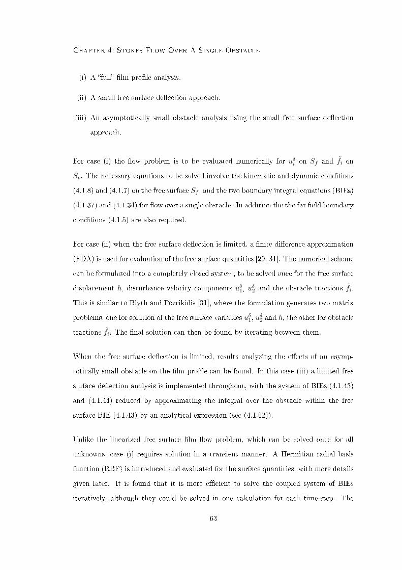
Chapter 4: Stokes Flow Over A Single Obstacle
(i) A full lm prole analysis.
(ii) A small free surface deection approach.
(iii) An asymptotically small obstacle analysis using the small free surface deection
approach.
For case (i) the ow problem is to be evaluated numerically for uδi on Sf and fi on
Sp. The necessary equations to be solved involve the kinematic and dynamic conditions
(4.1.8) and (4.1.7) on the free surface Sf , and the two boundary integral equations (BIEs)
(4.1.37) and (4.1.34) for ow over a single obstacle. In addition the the far eld boundary
conditions (4.1.5) are also required.
For case (ii) when the free surface deection is limited, a nite dierence approximation
(FDA) is used for evaluation of the free surface quantities [29, 31]. The numerical scheme
can be formulated into a completely closed system, to be solved once for the free surface
displacement h, disturbance velocity components uδ1, uδ2 and the obstacle tractions fi.
This is similar to Blyth and Pozrikidis [31], where the formulation generates two matrix
problems, one for solution of the free surface variables uδ1, uδ2 and h, the other for obstacle
tractions fi. The nal solution can then be found by iterating between them.
When the free surface deection is limited, results analyzing the eects of an asymp-
totically small obstacle on the lm prole can be found. In this case (iii) a limited free
surface deection analysis is implemented throughout, with the system of BIEs (4.1.43)
and (4.1.44) reduced by approximating the integral over the obstacle within the free
surface BIE (4.1.43) by an analytical expression (see (4.1.62)).
Unlike the linearized free surface lm ow problem, which can be solved once for all
unknowns, case (i) requires solution in a transient manner. A Hermitian radial basis
function (RBF) is introduced and evaluated for the surface quantities, with more details
given later. It is found that it is more ecient to solve the coupled system of BIEs
iteratively, although they could be solved in one calculation for each time-step. The
63
Chapter 4: Stokes Flow Over A Single Obstacle
iterative sequence used was:
(i) Guess an initial lm prole and disturbance velocities for the free surface.
(ii) Calculate the disturbance boundary traction using the dynamic condition (4.1.7).
(iii) Use the obstacle BIE (4.1.37) to calculate the boundary tractions on the obstacle,
fi.
(iv) Use the free surface BIE (4.1.34) to calculate a new set of disturbance velocities on
the lm surface.
(v) Via the kinematic condition (4.1.8) and using a forward nite dierence, the free
surface position is iterated in time.
(vi) Repeat from step 2 using the new lm prole and disturbance velocity prole for
the free surface, until the surface has reached a steady prole.
The BIEs were solved using a boundary element method (BEM) on the discretized sur-
faces and the implementation of this method is discussed below. In addition through the
remainder of this section, the use of FDAs and a Hermitian RBF for evaluating the free
surface curvature and outward unit normal are considered.
4.2.1 Surface Discretizations And The Boundary Element Method
For numerical solutions, the obstacle boundary and free surface require discretizing and
in this chapter, hemispherical and spherical objects were considered. The hemispherical
obstacle mesh is generated by a method of successive subdivision and consists of linear
triangular elements. Spherical obstacles were meshed by reective symmetry of the
hemispherical discretization. Figure 4.3 indicates typical meshes for the hemispherical
obstacles considered throughout this work.
64

Chapter 4: Stokes Flow Over A Single Obstacle
−1−0.5
00.5
1 −1−0.5
00.5
1−1
−0.9
−0.8
−0.7
−0.6
−0.5
−0.4
−0.3
−0.2
−0.1
x2
x1
x3
Figure 4.3: Typical mesh for a hemispherical obstacle of radius a = 0.9.
For the simplest case of small lm deection, the free surface is discretized using a set of
uniform, linear rectangular elements. However, when the free surface requires discretizing
fully, rectangular elements are insucient for the mesh and linear triangular elements
are used. Triangular elements were formed by rst subdividing the free surface domain
into a set of rectangular elements, and then for each element connecting the diagonal
vertices to form four sub-triangular linear elements. Free surface elements are referred to
as m× n, where for a rectangular mesh m is the number of elements in the x1 direction
and n the number of elements in the x2 direction. For a triangular mesh of m× n, the
free surface is rst divided into a m/2× n/2 rectangular mesh and further subdivisions
to create the triangular elements are carried out as described above. A schematic of
typical free surface discretizations using rectangular and triangular elements are shown
in gure 4.4.
The BEM was used to solve each of the BIEs within the problem. The velocity and
traction variables were assumed constant over each element, and values assigned at the
65

Chapter 4: Stokes Flow Over A Single Obstacle
Figure 4.4: Typical mesh for the free surface using (a) rectangular elements, and (b)
triangular elements.
midpoint of the elements. To avoid diculty in the re-meshing of the surface with
every time-step the velocities and tractions were found at the element midpoints and
these midpoints are repositioned in the x3 direction at every time step. Movement
of the element nodal points was achieved by tting a Hermitian RBF through the new
midpoints and nding the corresponding new nodal locations for each element. It is noted
that the data point is displaced from the new linear elements midpoint and a small error
occurs within the BEM approximation. Globally the accurate midpoint heights are used
when evaluating the kinematic and dynamic boundary conditions, but the approximated
midpoint heights (from the linear element mesh) are used for collocation within the
BEM.
4.2.2 Integration Techniques And Near Point Singularities
Standard numerical integration regimes for the stress and velocity Green's functions over
the linear elements were conducted. A 4-point Gaussian quadrature scheme was used for
the rectangular elements and 3-point for the triangular elements. The velocity Green's
66

Chapter 4: Stokes Flow Over A Single Obstacle
function on singular elements was integrated using the polar integration rule. For larger
obstacles that approach the free surface, the BIEs eventually fail numerically due to
near-point singularities. This problem is common when modelling thin structures and
gaps using conventional BEMs. As outlined by Krishnasamy et al. [49], two diculties
arise from the standard BIEs when considering thin bodies. These are,
(i) As the gap between two surfaces reduces, the BIEs tend to form an ill condition
coecient matrix.
(ii) The integrals become nearly singular and dicult to evaluate accurately using
standard numerical integration schemes.
Krishnasamy et al. [49] notes that achieving a suitable integration technique to solve the
problem of nearly singular integrals allows limited success with thin shapes. For very
thin shapes, the ill conditioning eventually becomes too severe for the conventional BIE
to be applicable in solving the problem. However for the lm ows considered in this
paper, the severity of reduced thickness necessary to cause ill-conditioning eects are
physically unrealistic.
Several techniques are reported in the literature to deal with near-singular integration.
They include element subdivision Lachat and Watson [50], adaptive Gaussian integration
Hayami [51], variable transformation techniques and semi-analytical integration based
on series expansions and removal of singularities, Mi and Aliabadi [52], besides others.
In this work, the eects of ill conditioning are not considered and improvements in the
numerical integration scheme follow a method similar to that outlined in Cutanda et al.
[53], and consists of a combination of the adaptive Gaussian integration algorithm and
the element subdivision approach. The approach of Cutanda et al. [53] to deal with
near-singular integrals was chosen due to its simplicity of formulation, although it is
known that some other approaches, such as variable transformation and semi-analytical
integration, are numerically more ecient.
67
Chapter 4: Stokes Flow Over A Single Obstacle
The distance, d, between the singular point and the linear triangular element of inte-
gration was rst evaluated. Standard integration was conducted via a 3-point triangular
Gaussian quadrature method. Integration renement was used depending on the dis-
tance d and the successive threshold distances as shown in table 4.2. If the distance was
below a certain threshold, d1, then 6-point triangular Gaussian quadrature was used. If
the distance was less than d2, 9-point Gaussian integration was used and if the distance
was less than d3, 13-point Gaussian integration was used.
However, increasing the order of integration gives only limited improvement on the thin-
ness of gap that can be modelled [53]. Using the 13-point integration technique, a
method of subdivision is required. The method chosen followed a similar manner to the
geometrical successive sub-division used in discretizing the hemispherical and spherical
obstacles. If the distance between the integration element and singularity was less than
d4, then the element was split into four theoretical sub elements. The distance between
each sub element and the singularity was then tested and if less than a distance d5, then
the sub element is split into four theoretical sub-sub triangular elements. This method is
repeated for up to ve consecutive sub divisions and if the whole element was discretized
to the maximum it would be sub-divided into 45 integration regions. This has the added
benet of only increasing the numerical computation in the required regions.
This approach requires nding suitable values for the distances di where i = 1, . . . , 8 and
the values used are shown in table 4.2 after an extensive convergence analysis has been
conducted. The computational time associated with calculating the distance between
element and singularity and subsequent adjustments was not excessive on the compu-
tational run-time of the simulation and is signicantly advantageous over using a high
order integration technique applied for all elements.
68
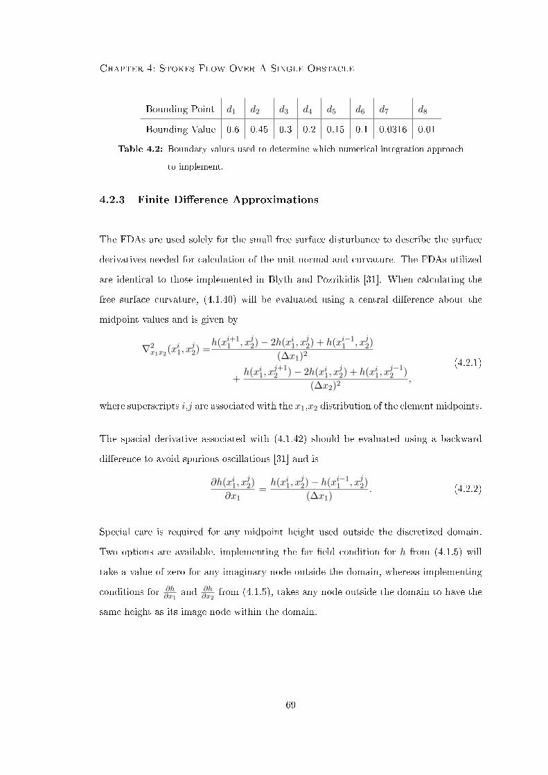
Chapter 4: Stokes Flow Over A Single Obstacle
Bounding Point d1 d2 d3 d4 d5 d6 d7 d8
Bounding Value 0.6 0.45 0.3 0.2 0.15 0.1 0.0316 0.01
Table 4.2: Boundary values used to determine which numerical integration approach
to implement.
4.2.3 Finite Dierence Approximations
The FDAs are used solely for the small free surface disturbance to describe the surface
derivatives needed for calculation of the unit normal and curvature. The FDAs utilized
are identical to those implemented in Blyth and Pozrikidis [31]. When calculating the
free surface curvature, (4.1.40) will be evaluated using a central dierence about the
midpoint values and is given by
∇2x1x2
(xi1, xj2) =
h(xi+11 , xj2)− 2h(xi1, x
j2) + h(xi−1
1 , xj2)(∆x1)2
+h(xi1, x
j+12 )− 2h(xi1, x
j2) + h(xi1, x
j−12 )
(∆x2)2,
(4.2.1)
where superscripts i,j are associated with the x1,x2 distribution of the element midpoints.
The spacial derivative associated with (4.1.42) should be evaluated using a backward
dierence to avoid spurious oscillations [31] and is
∂h(xi1, xj2)
∂x1=h(xi1, x
j2)− h(xi−1
1 , xj2)(∆x1)
. (4.2.2)
Special care is required for any midpoint height used outside the discretized domain.
Two options are available, implementing the far eld condition for h from (4.1.5) will
take a value of zero for any imaginary node outside the domain, whereas implementing
conditions for ∂h∂x1
and ∂h∂x2
from (4.1.5), takes any node outside the domain to have the
same height as its image node within the domain.
69

Chapter 4: Stokes Flow Over A Single Obstacle
4.2.4 Finite Free Surface Deections And Radial Basis Functions
For nite free surface deections, accurate evaluation of the unit normal and curvature
as dened in equations (4.1.11) and (4.1.12) using FDAs is dicult. Thus a RBF can
be used to interpolate a set of data points contained within a domain, and by use of a
Hermite RBF the boundary conditions also applied. At any point on the free surface, the
height is given by h(x1, x2), and takes values hi at data point i for a total of N points.
The surface can then be interpolated using the RBF ψ(‖x − ξj‖), where j = 1, . . . , N
and ξj are the x1, x2 co-ordinates of the data points hj .
A choice of thin plate splines was used for the RBF. The addition of a polynomial is
required to guarantee invertibility when using a thin plate spline since it is known that the
generalized thin plate spline of power (2m−2) is a conditionally positive denite function
of order m. Thus it requires the addition of a polynomial term of order m− 1, together
with a homogeneous constraint condition, in order to obtain an invertible interpolation
matrix. In our case, we are using m = 3 requiring a second order polynomial and the
thin plate spline RBF takes the form
ψ = r2m−2 log r, (4.2.3)
where
r = ‖x− ξ‖. (4.2.4)
A value of m = 3 avoids singularities at r = 0 for up to and including the third order
derivatives of ψ and as stated in La Rocca et al. [41] minimizes the interpolation matrix
becoming more ill-conditioned.
The values of ∂h∂x1
and ∂h∂x2
can be constrained at a selected set of n data points (such as
the far eld locations where the gradients are set to zero), whilst still dening h on the
original N data points. A solution for h can be obtained using the dierential operators
∂∂x1
and ∂∂x2
but acting on the thin plate splines second argument ξ, i.e. ∂∂ξ1
and ∂∂ξ2
. A
70
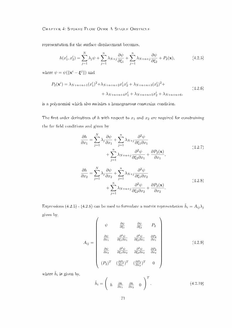
Chapter 4: Stokes Flow Over A Single Obstacle
representation for the surface displacement becomes,
h(xi1, xi2) =
N∑j=1
λjψ +n∑j=1
λN+j∂ψ
∂ξ1+
n∑j=1
λN+n+j∂ψ
∂ξ2+ P2(x), (4.2.5)
where ψ = ψ(‖xi − ξj‖) and
P2(xi) = λN+n+n+1(xi1)2+λN+n+n+2xi1xi2 + λN+n+n+3(xi2)2+
+ λN+n+n+4xi1 + λN+n+n+5x
i2 + λN+n+n+6,
(4.2.6)
is a polynomial which also satises a homogeneous constraint condition.
The rst order derivatives of h with respect to x1 and x2 are required for constraining
the far eld conditions and given by
∂h
∂x1=
N∑j=1
λj∂ψ
∂x1+
n∑j=1
λN+j∂2ψ
∂ξ1∂x1
+n∑j=1
λN+n+j∂2ψ
∂ξ2∂x1+∂P2(x)∂x1
,
(4.2.7)
∂h
∂x2=
N∑j=1
λj∂ψ
∂x2+
n∑j=1
λN+j∂2ψ
∂ξ1∂x2
+n∑j=1
λN+n+j∂2ψ
∂ξ2∂x2+∂P2(x)∂x2
.
(4.2.8)
Expressions (4.2.5) - (4.2.8) can be used to formulate a matrix representation hi = Aijλj
given by,
Aij =
ψ ∂ψ∂ξ1
∂ψ∂ξ2
P2
∂ψ∂x1
∂2ψ∂ξ1∂x1
∂2ψ∂ξ2∂x1
∂P2∂x1
∂ψ∂x2
∂2ψ∂ξ1∂x2
∂2ψ∂ξ2∂x2
∂P2∂x2
(P2)T (∂P2∂x1
)T (∂P2∂x2
)T 0
(4.2.9)
where hi is given by,
hi =
(h ∂h
∂x1
∂h∂x2
0
)T. (4.2.10)
71
Chapter 4: Stokes Flow Over A Single Obstacle
This system must be solved to nd the vector λj .
Once the system has been solved for λj , the RBF can be evaluated for the outward
unit normal and mean curvature of the free surface. Evaluation of the unit normal will
require derivatives ∂h∂x1
and ∂h∂x2
, with the mean curvature needing in addition, ∂2h∂x2
1, ∂
2h∂x2
2,
and ∂2h∂x1∂x2
on the surface. The evaluation of these derivatives simply involve the nding
of specic derivatives of ψ. The values of h, ∂h∂x1
and ∂h∂x2
are determined by (4.2.5) -
(4.2.8). The corresponding second order derivatives are given by
∂2h
∂x21
=N∑j=1
λj∂2ψ
∂x21
+n∑j=1
λN+j∂3ψ
∂ξ1∂x21
+n∑j=1
λN+n+j∂3ψ
∂ξ2∂x21
+∂2P2(x)∂x2
1
,
(4.2.11)
∂2h
∂x22
=N∑j=1
λj∂2ψ
∂x21
+n∑j=1
λN+j∂3ψ
∂ξ1∂x22
+n∑j=1
λN+n+j∂3ψ
∂ξ2∂x22
+∂2P2(x)∂x2
2
,
(4.2.12)
∂2h
∂x1∂x2=
N∑j=1
λj∂2ψ
∂x1∂x2+
n∑j=1
λN+j∂3ψ
∂ξ1∂x1∂x2
+n∑j=1
λN+n+j∂3ψ
∂ξ2∂x1∂x2+∂2P2(x)∂x1∂x2
.
(4.2.13)
When implementing the thin plate spline RBF (4.2.3) for the interpolation of the free
surface, the following derivatives of ψ are required
∂ψ
∂ξ1= −r2(2 log (r2) + 1)(x1 − ξ1), (4.2.14)
∂ψ
∂ξ2= −r2(2 log (r2) + 1)(x2 − ξ2), (4.2.15)
∂ψ
∂x1= r2(2 log (r2) + 1)(x1 − ξ1), (4.2.16)
∂ψ
∂x2= r2(2 log (r2) + 1)(x2 − ξ2), (4.2.17)
∂2ψ
∂ξ1∂x1= −(x1 − ξ1)2(4 log (r2) + 6)− r2(2 log (r2) + 1), (4.2.18)
72
Chapter 4: Stokes Flow Over A Single Obstacle
∂2ψ
∂ξ2∂x1= −(x1 − ξ1)(x2 − ξ2)(4 log (r2) + 6), (4.2.19)
∂2ψ
∂ξ1∂x2= −(x1 − ξ1)(x2 − ξ2)(4 log (r2) + 6), (4.2.20)
∂2ψ
∂ξ2∂x2= −(x2 − ξ2)2(4 log (r2) + 6)− r2(2 log (r2) + 1), (4.2.21)
∂2ψ
∂x21
= r2(2 log (r2) + 1) + (x1 − ξ1)2(4 log (r2) + 6), (4.2.22)
∂2ψ
∂x22
= r2(2 log (r2) + 1) + (x2 − ξ2)2(4 log (r2) + 6), (4.2.23)
∂2ψ
∂x1∂x2= (x2 − ξ2)(x1 − ξ1)(4 log (r2) + 6), (4.2.24)
∂3ψ
∂ξ1∂x21
= −3(x1 − ξ1)(4 log (r2) + 6)− 8(x1 − ξ1)3
r2, (4.2.25)
∂3ψ
∂ξ2∂x21
= −(x2 − ξ2)(
4 log (r2) + 6 + 8(x1 − ξ1)2
r2
), (4.2.26)
∂3ψ
∂ξ1∂x22
= −(x1 − ξ1)(
4 log (r2) + 6 + 8(x2 − ξ2)2
r2
), (4.2.27)
∂3ψ
∂ξ2∂x22
= −3(x2 − ξ2)(4 log (r2) + 6)− 8(x2 − ξ2)3
r2, (4.2.28)
∂3ψ
∂ξ1∂x1∂x2= −(x2 − ξ2)
(4 log (r2) + 6 + 8
(x1 − ξ1)2
r2
), (4.2.29)
∂3ψ
∂ξ2∂x1∂x2= −(x1 − ξ1)
(4 log (r2) + 6 + 8
(x2 − ξ2)2
r2
). (4.2.30)
4.3 Solution Proles For Flow Over An Obstacle
Simulations of ow computations over single obstacles and corresponding numerical de-
tails are described in this section, each identifying dierent aspects of the numerical
method.
Results are initially produced illustrating the eects of implementing a Hermitian radial
basis function (RBF) for the free surface compared with the nite dierence approxima-
tions (FDAs) used in [29, 31]. Blyth and Pozrikidis [31] produced gures for an inverse
73

Chapter 4: Stokes Flow Over A Single Obstacle
Bond number B, related to Bo by
Bo =sin1/3 α
B, (4.3.1)
and to allow comparison of results, appropriate solutions are given in terms of the inverse
Bond number B. Results are also reproduced from Blyth and Pozrikidis [31], using a
global RBF with the limitation of a small amplitude free surface deection and the
asymptotic obstacle analysis where appropriate. Consistency of results is found between
the full obstacle and asymptotic analysis.
The assumption of small free surface deection is then removed and results for the
nite deection approach presented for signicant lm deformations generated by large
hemispherical obstacles. An example of particular interest is where the uid lm can
fully contain an obstacle that is taller than the undisturbed lm height.
4.3.1 Small Free Surface Deections
This section considers implementation of a global Hermitian RBF for nding the unit
normal and curvature of the free surface. Comparisons are made with the FDAs used
in the published work by Pozrikidis and Thoroddsen [29] and Blyth and Pozrikidis [31].
Flow down an inclined plane over a hemispherical obstacle is considered using the small
free surface deection restriction. The RBF analysis is to be solved transiently, to con-
verge to a steady state prole. For illustration, calculation is taken for ow over hemi-
spherical obstacles of radius a = 0.2, a Bond number of Bo = 0.89, (B = 1) and the
plane is inclined at α = 45o. A suitable choice for the size of the free surface domain
is required such that the far eld conditions (4.1.5) are accurately represented on the
edges of the domain. The choice of free surface domain was made by initially solving
the problem for large far eld distances, and progressively reducing these truncation
points. The optimum free surface domain was one that minimized the area that required
discretization, whilst maintaining accurate representation of the free surface prole. For
this ow problem, it was found that the free surface should be solved within the domain
74
Chapter 4: Stokes Flow Over A Single Obstacle
−6 ≤ x1 ≤ 8, −6 ≤ x2 ≤ 6. Similar analysis are conducted to nd suitable far eld
truncation values when other ow parameters are chosen. The hemispherical obstacle
was discretized using 256 linear triangular elements in all cases, with the level of free
surface discretization varied between results. The far eld boundary condition of zero
gradients was imposed throughout. For consistency with the FDAs, the far eld condi-
tion was applied at the element midpoints within the RBF of any element containing a
boundary node. This implementation will be improved for later results. Solutions are
interpolated to the centre line using a cubic spline for the FDA implementation and the
global RBF interpolation when implemented for the normal and curvature. A 4-point
Gaussian quadrature is used for the numerical integration over rectangular elements,
with a 3-point scheme implemented over triangular elements.
Figure 4.5a illustrates the centre line solutions for a free surface mesh resolution of 56×48.
The solutions are produced using both a RBF and FDA analysis for the free surface
normal and curvature. The main dierence between the RBF and FDA solution is the
dierence in peak height and trough depth. In addition, there is a marginal shift of the
centre line prole downstream when using the RBF interpolation. Figure 4.5b illustrates
the dierence in surface position along the centre line for two free surface rectangular
mesh resolutions, 56 × 48 and 28 × 24. The solutions for the two RBF meshes seem to
compare more favourably than the corresponding solutions found when implementing
FDAs. The RBF interpolation predicts the surface almost identically (especially in the
far eld), regardless of which resolution of mesh is used for the BIEs. The FDA solution
seems to exhibit a marginal shift downstream with increase in mesh resolution, with the
peak slightly higher.
Corresponding to Figure 4.5, a full three-dimensional prole for the RBF solution of
ow over a hemisphere using the more rened mesh of 56 × 48 elements is shown in
Figure 4.6. As expected the ow prole is symmetric, producing a large upstream peak,
which collapses into a shallow trough downstream of the obstacle. The peak decays in a
horseshoe shape fashion.
75
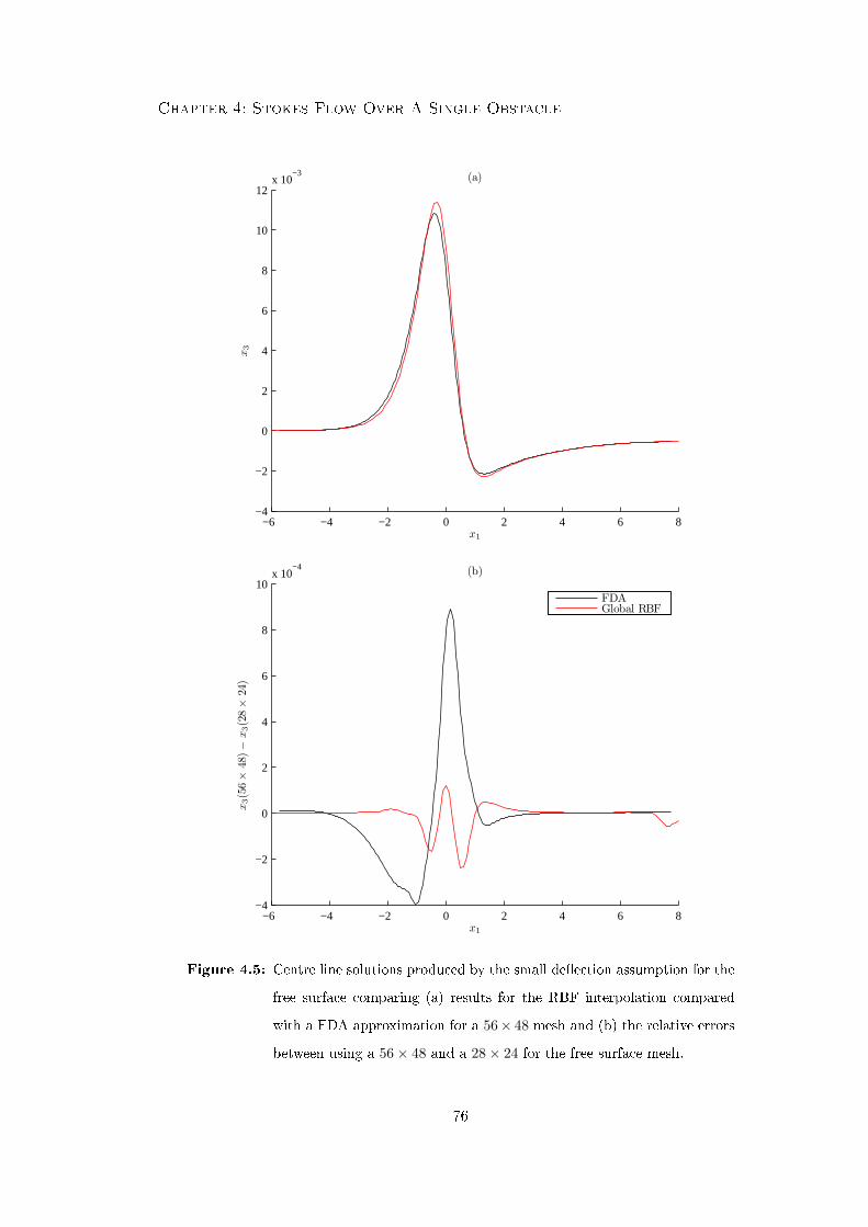
Chapter 4: Stokes Flow Over A Single Obstacle
−6 −4 −2 0 2 4 6 8−4
−2
0
2
4
6
8
10
12x 10
−3 (a)
x1
x3
−6 −4 −2 0 2 4 6 8−4
−2
0
2
4
6
8
10x 10
−4 (b)
x1
x3(5
6×
48)−
x3(2
8×
24)
FDAGlobal RBF
Figure 4.5: Centre line solutions produced by the small deection assumption for the
free surface comparing (a) results for the RBF interpolation compared
with a FDA approximation for a 56× 48 mesh and (b) the relative errors
between using a 56× 48 and a 28× 24 for the free surface mesh.
76
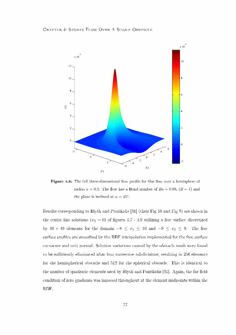
Chapter 4: Stokes Flow Over A Single Obstacle
Figure 4.6: The full three-dimensional ow prole for lm ow over a hemisphere of
radius a = 0.2. The ow has a Bond number of Bo = 0.89, (B = 1) and
the plane is inclined at α = 45o.
Results corresponding to Blyth and Pozrikidis [31] (their Fig 10 and Fig 8) are shown in
the centre line solutions (x2 = 0) of gures 4.7 - 4.9 utilizing a free surface discretized
by 49 × 49 elements for the domain −8 ≤ x1 ≤ 10 and −9 ≤ x2 ≤ 9. The free
surface proles are smoothed by the RBF interpolation implemented for the free surface
curvature and unit normal. Solution variations caused by the obstacle mesh were found
to be suciently eliminated after four successive subdivisions, resulting in 256 elements
for the hemispherical obstacle and 512 for the spherical obstacle. This is identical to
the number of quadratic elements used by Blyth and Pozrikidis [31]. Again, the far eld
condition of zero gradients was imposed throughout at the element midpoints within the
RBF.
77

Chapter 4: Stokes Flow Over A Single Obstacle
−8 −6 −4 −2 0 2 4 6 8 10
−2
0
2
4
6
8
10
12x 10
−3
x1(x2 = 0)
x3
B = 1B = 5B = 10B = 15B = 20
Figure 4.7: Centre line solutions for a selection of inverse Bond numbers, using the
assumption of small free surface deection. The plane is inclined at 45o
and the hemispherical obstacle has radius a = 0.2.
Figure 4.7 allows comparison with Blyth and Pozrikidis [31] (their Fig 10a) for ow down
an inclined plane at 45o over a hemisphere of radius a = 0.2. As the inverse Bond number
is increased, surface tension forces are increased in comparison to the gravitational forces
and acts to atten any surface deformation. With this increase in the value of B the peak
of the ow appears to migrate slightly upstream. A comparison to the results of Blyth
and Pozrikidis [31] (their Fig 10a) shows that, although the qualitative behaviour is the
same, current results exhibit a larger peak. Taking B = 1, the percentage dierence of
peak heights between the FDA and RBF models is approximately 24% as estimated from
the FDA solution presented in [31]. It is thought that this dierence in the lm prole
is caused by the diering far eld conditions used within the FDA of [31] and the RBF
analysis presented in this Thesis. Within [31] the zero deection far eld condition is
implemented, which can cause irregularities of the lm prole at the far eld truncation
78

Chapter 4: Stokes Flow Over A Single Obstacle
−8 −6 −4 −2 0 2 4 6 8 10
−2
0
2
4
6
8
10
12
14x 10
−3
x1(x2 = 0)
x3
α = 90o
α = 45o
α = 27o
α = 9o
Figure 4.8: Centre line solutions for a selection of wall inclinations, using the assump-
tion of small free surface deection. The ow has an inverse Bond number
B = 1 and the hemispherical obstacle has radius a = 0.2.
point if the condition is not suciently satised. This problem is eliminated by using
the zero derivative condition within the RBF analysis, which oers a more consistent
approximation in the far eld. Implementing the zero derivative far eld condition within
both the FDA and RBF method, yields more consistent results as can be seen in gure
4.5a.
Figure 4.8 illustrates solutions for a selection of inclination angles for a ow with an
inverse Bond number B = 1 and hemispherical obstacle of radius a = 0.2. Increasing the
inclination angle has the eect of increasing the peak size and decreasing the trough size
behind the obstacle. Although the peak location is relatively unaected by the inclination
angles, the downstream trough is seen to migrate upstream as the angle is reduced. This
is in agreement with Blyth and Pozrikidis [31] (their Fig10b) as a direct comparison with
this work. Again it is seen that results in gure 4.8 using the RBF interpolation exhibit
79

Chapter 4: Stokes Flow Over A Single Obstacle
−8 −6 −4 −2 0 2 4 6 8 10
−0.02
0
0.02
0.04
0.06
0.08
0.1
0.12
0.14
0.16
x1(x2 = 0)
x3
a = 0.2a = 0.4a = 0.6
Figure 4.9: Centre line solutions for a selection of hemisphere radii, using the as-
sumption of small free surface deection. The ow has an inverse Bond
number B = 1 and is along an inclined plane at 45o.
a larger peak then those in [31]. The percentage dierence of peak heights for α = 90o
between the RBF and FDA models is approximately 18%, obtained by estimation of the
FDA lm prole from [31]. As for gure 4.7, these dierences are likely to be caused
by the dierent far eld conditions implemented in [31] and this Thesis. In particular,
where the zero deection approximation is used [31], possible irregularities in the lm
prole can occur in the far eld. These irregularities are not seen when using the zero
derivative far eld constraint as used within the RBF interpolation.
Figure 4.9 illustrates solutions for small to large obstacle sizes for a ow with an inverse
Bond number B = 1 on an inclined plane at an angle of 45o. Here, as expected, a larger
obstacle will generate a larger deformation. Again results are in direct comparison with
the plot by Blyth and Pozrikidis [31] (their Fig 8). The peaks of the RBF analysis appear
larger than those using FDAs, and the percentage dierence of peak height between the
80
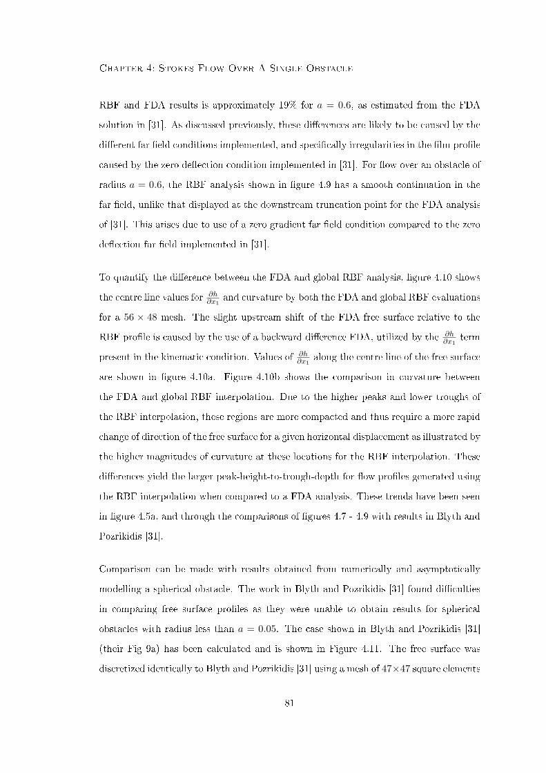
Chapter 4: Stokes Flow Over A Single Obstacle
RBF and FDA results is approximately 19% for a = 0.6, as estimated from the FDA
solution in [31]. As discussed previously, these dierences are likely to be caused by the
dierent far eld conditions implemented, and specically irregularities in the lm prole
caused by the zero deection condition implemented in [31]. For ow over an obstacle of
radius a = 0.6, the RBF analysis shown in gure 4.9 has a smooth continuation in the
far eld, unlike that displayed at the downstream truncation point for the FDA analysis
of [31]. This arises due to use of a zero gradient far eld condition compared to the zero
deection far eld implemented in [31].
To quantify the dierence between the FDA and global RBF analysis, gure 4.10 shows
the centre line values for ∂h∂x1
and curvature by both the FDA and global RBF evaluations
for a 56 × 48 mesh. The slight upstream shift of the FDA free surface relative to the
RBF prole is caused by the use of a backward dierence FDA, utilized by the ∂h∂x1
term
present in the kinematic condition. Values of ∂h∂x1
along the centre line of the free surface
are shown in gure 4.10a. Figure 4.10b shows the comparison in curvature between
the FDA and global RBF interpolation. Due to the higher peaks and lower troughs of
the RBF interpolation, these regions are more compacted and thus require a more rapid
change of direction of the free surface for a given horizontal displacement as illustrated by
the higher magnitudes of curvature at these locations for the RBF interpolation. These
dierences yield the larger peak-height-to-trough-depth for ow proles generated using
the RBF interpolation when compared to a FDA analysis. These trends have been seen
in gure 4.5a, and through the comparisons of gures 4.7 - 4.9 with results in Blyth and
Pozrikidis [31].
Comparison can be made with results obtained from numerically and asymptotically
modelling a spherical obstacle. The work in Blyth and Pozrikidis [31] found diculties
in comparing free surface proles as they were unable to obtain results for spherical
obstacles with radius less than a = 0.05. The case shown in Blyth and Pozrikidis [31]
(their Fig 9a) has been calculated and is shown in Figure 4.11. The free surface was
discretized identically to Blyth and Pozrikidis [31] using a mesh of 47×47 square elements
81

Chapter 4: Stokes Flow Over A Single Obstacle
−6 −4 −2 0 2 4 6 8−0.02
−0.015
−0.01
−0.005
0
0.005
0.01(a)
x1(x2 = 0)
∂h
∂x1
−6 −4 −2 0 2 4 6 8−0.02
−0.01
0
0.01
0.02
0.03
0.04(b)
x1(x2 = 0)
curv
atur
e,κ
FDAGlobal RBF
Figure 4.10: Centre line solutions comparing (a) ∂h∂x1
and (b) the curvature κ, for the
ow proles with a 56 × 48 mesh as shown in gure 4.5. Both cases
utilize the small free surface deection assumption.
82

Chapter 4: Stokes Flow Over A Single Obstacle
for the asymptotic results and 49× 49 square elements for the complete analysis over a
truncated domain of −8 ≤ x1 ≤ 10, −9 ≤ x2 ≤ 9. Again the midpoint values of surface
height are interpolated using the RBF implemented for the free surface curvature and
unit normal to produce a smooth curve. The zero gradient far eld condition was used
throughout.
The ow is solved for a plane inclination angle of 45o with inverse Bond number B = 1.
Figure 4.11 compares centre line results for a radius of a = 0.05. As in Blyth and
Pozrikidis [31] the asymptotic solution is found to over-predict the maximum displace-
ment compared to the solution obtained by numerical analysis of the sphere. However
the larger peak heights found from the current approach provides a closer t between
the asymptotic and numerical results. The centre lines of the asymptotic solutions us-
ing a RBF interpolation still over-predict the published results in Blyth and Pozrikidis
[31] (their Fig 9a) utilizing FDAs, although the dierences appear smaller than those
for numerical results obtained. It is also noted that no limitations on the size of a are
present for our numerical model. Figure 4.12 illustrates centre line solution for a = 0.001
with the asymptotic and numerical solutions giving near identical results. A small 1.5%
dierence in peak heights along the centre line is found, indicating consistency between
the two models.
4.3.2 Large Free Surface Deections
Results generated by removing the small amplitude free surface deection approximation
from Blyth and Pozrikidis [31] are produced in this section. A global RBF scheme is used
for calculation of the free surface parameters, and implements the zero derivative far eld
conditions applied at the element nodes on the boundary of the domain. When using a
large free surface deection analysis, the free surface is meshed using triangular elements
in preference to the rectangular elements used for the small free surface deections. Mesh
renements are considered for a domain of −6 ≤ x1 ≤ 8 and −6 ≤ x2 ≤ 6 discretized
83

Chapter 4: Stokes Flow Over A Single Obstacle
−8 −6 −4 −2 0 2 4 6 8 10−4
−2
0
2
4
6
8
10
12
14x 10
−4
x1(x2 = 0)
x3
Asymptotic AnalysisNumerical Analysis
Figure 4.11: Centre line surface proles using the assumption of small free surface
deection for ow over a sphere of radius a = 0.05 using an asymptotic
and numerical analysis for the sphere.
by both 28 × 24 and 56 × 48 elements. A small hemispherical obstacle of radius 0.2
is considered and the ow is down a plane inclined at α = 45o with an inverse Bond
number B = 1. Centre line solutions indicating the prole for the 56× 48 mesh, and the
error between this and the coarser mesh are shown in gure 4.13.
The validity of the small free surface deection assumption is analyzed by direct com-
parisons of results for large and small deections, caused by large and small obstacles
respectively. Again, a domain of −6 ≤ x1 ≤ 8 and −6 ≤ x2 ≤ 6 is considered for the
free surface, discretized by 28× 24 elements as found sucient above. The small hemi-
spherical obstacle has a radius of 0.2 and the large hemisphere a radius of 0.9. Both are
discretized by successive subdivision into 256 geometrically linear elements. The ow is
down a plane inclined at α = 45o with an inverse Bond number B = 1. For direct com-
parison with earlier results, the near point singularity analysis is omitted, with numerical
84
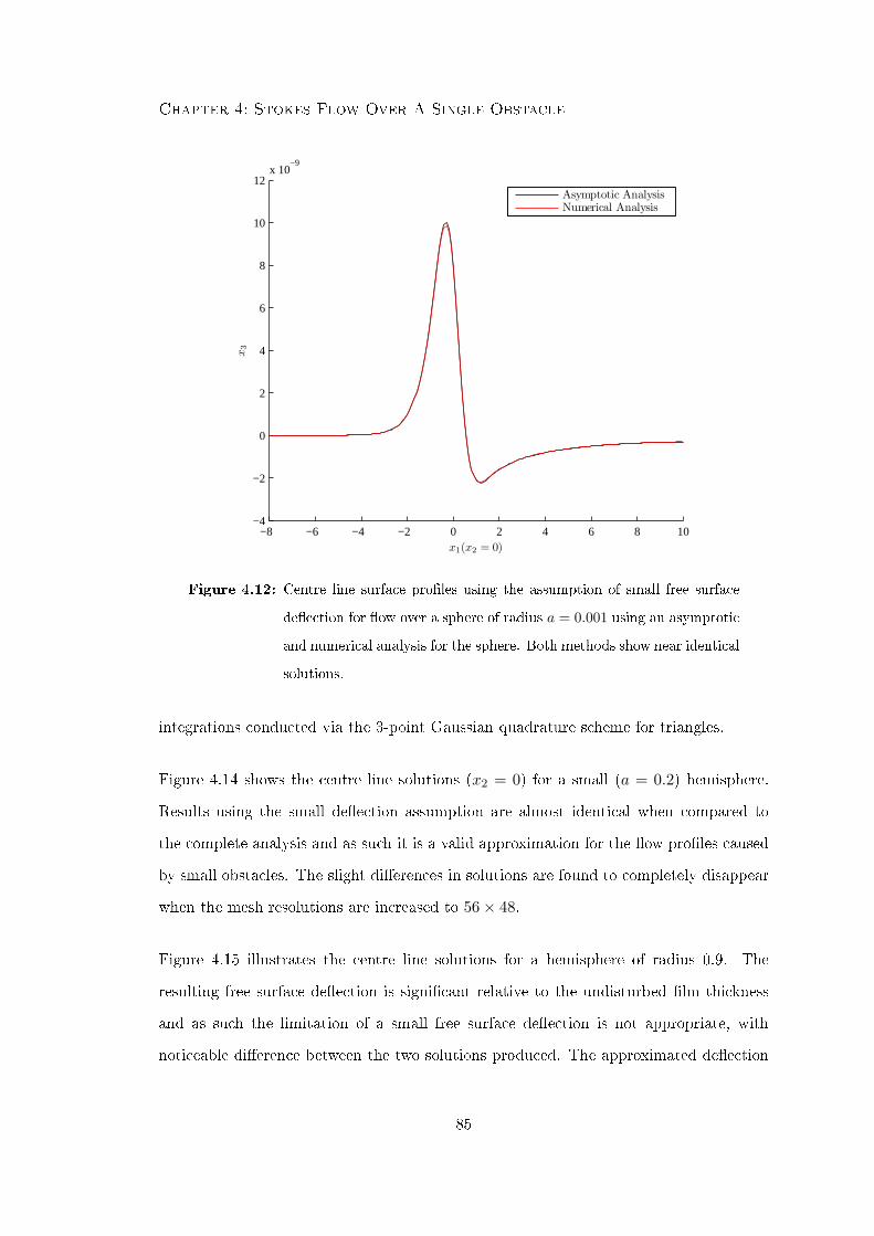
Chapter 4: Stokes Flow Over A Single Obstacle
−8 −6 −4 −2 0 2 4 6 8 10−4
−2
0
2
4
6
8
10
12x 10
−9
x1(x2 = 0)
x3
Asymptotic AnalysisNumerical Analysis
Figure 4.12: Centre line surface proles using the assumption of small free surface
deection for ow over a sphere of radius a = 0.001 using an asymptotic
and numerical analysis for the sphere. Both methods show near identical
solutions.
integrations conducted via the 3-point Gaussian quadrature scheme for triangles.
Figure 4.14 shows the centre line solutions (x2 = 0) for a small (a = 0.2) hemisphere.
Results using the small deection assumption are almost identical when compared to
the complete analysis and as such it is a valid approximation for the ow proles caused
by small obstacles. The slight dierences in solutions are found to completely disappear
when the mesh resolutions are increased to 56× 48.
Figure 4.15 illustrates the centre line solutions for a hemisphere of radius 0.9. The
resulting free surface deection is signicant relative to the undisturbed lm thickness
and as such the limitation of a small free surface deection is not appropriate, with
noticeable dierence between the two solutions produced. The approximated deection
85
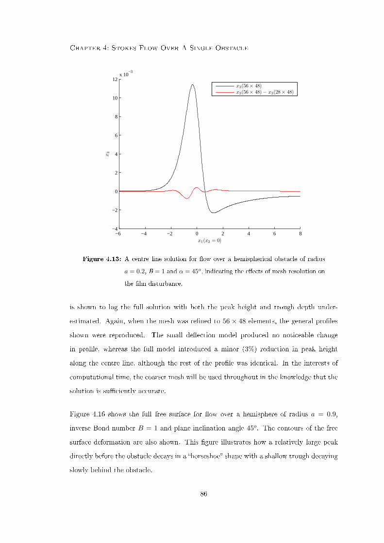
Chapter 4: Stokes Flow Over A Single Obstacle
−6 −4 −2 0 2 4 6 8−4
−2
0
2
4
6
8
10
12x 10
−3
x1(x2 = 0)
x3
x3(56× 48)x3(56× 48)− x3(28× 48)
Figure 4.13: A centre line solution for ow over a hemispherical obstacle of radius
a = 0.2, B = 1 and α = 45o, indicating the eects of mesh resolution on
the lm disturbance.
is shown to lag the full solution with both the peak height and trough depth under-
estimated. Again, when the mesh was rened to 56 × 48 elements, the general proles
shown were reproduced. The small deection model produced no noticeable change
in prole, whereas the full model introduced a minor (3%) reduction in peak height
along the centre line, although the rest of the prole was identical. In the interests of
computational time, the coarser mesh will be used throughout in the knowledge that the
solution is suciently accurate.
Figure 4.16 shows the full free surface for ow over a hemisphere of radius a = 0.9,
inverse Bond number B = 1 and plane inclination angle 45o. The contours of the free
surface deformation are also shown. This gure illustrates how a relatively large peak
directly before the obstacle decays in a horseshoe shape with a shallow trough decaying
slowly behind the obstacle.
86

Chapter 4: Stokes Flow Over A Single Obstacle
−6 −4 −2 0 2 4 6 8
−2
0
2
4
6
8
10
12x 10
−3
x1(x2 = 0)
x3
Small Deflection ApproximationFull Deflection Model
Figure 4.14: Comparison of centre line solutions for ow over a hemispherical obstacle
with and without the small free surface deection assumption. Flow
parameters are a = 0.2, B = 1 and α = 45o.
Figure 4.17 illustrates the streamlines for ow over a hemisphere attached to an inclined
plane at 45o. The hemisphere has a radius of a = 0.9 and the ow has an inverse Bond
number of B = 1. The two innermost streamlines move both outward, as well as over
the hemisphere and streamline deection reduces considerably further from the obstacle.
It is noted that solutions show symmetry in the plane x2 = 0.
Following Blyth and Pozrikidis [31], comparisons of the centre line solutions for a pa-
rameter analysis of the inverse Bond number and plane inclination angle is conducted.
The obstacle is a hemisphere of radius a = 0.9 and discretized by 256 elements. A ow
domain of −8 ≤ x1 ≤ 10 and −8 ≤ x2 ≤ 8 is considered with free surface meshes
consisting of element distributions of 36 × 32. Again integration omits the near point
singularity analysis and a 3-point Gaussian quadrature scheme is used.
87

Chapter 4: Stokes Flow Over A Single Obstacle
−6 −4 −2 0 2 4 6 8−0.1
−0.05
0
0.05
0.1
0.15
0.2
0.25
0.3
0.35
0.4
x1(x2 = 0)
x3
Small Deflection AnalysisFull Deflection Model
Figure 4.15: Comparison of centre line solutions for ow over a hemispherical obstacle
with and without the small free surface deection assumption. Flow
parameters are a = 0.9, B = 1 and α = 45o.
Figure 4.18a indicates solutions for a range of inverse Bond numbers B and is comparable
to the small deection results of gure 4.7. Flow is down a 45o plane and as expected
increasing the inverse Bond number results in a attening and smoothing of the inter-
face. The peak is also seen to migrate slightly upstream. Within gure 4.18a, the far
eld condition appears not to be satised and this is a direct consequence of the size of
the truncated domain used for calculation and the extended distances required for high
surface tension ows to return fully to the undisturbed prole. However, the implemen-
tation of the zero derivative boundary condition helps retain consistent results without
signicant deections caused by forcing an unrealistic far eld condition. Figure 4.18b
indicates the correlation between the maximum and minimum lm height and inverse
Bond number B corresponding to the results of gure 4.18a. Clearly the magnitude of
the deection from zero is reduced in both cases as B is increased, appearing to tend
towards constant values for the maximum and minimum deection. Peak height is af-
88

Chapter 4: Stokes Flow Over A Single Obstacle
Figure 4.16: Three-dimensional solution prole for ow over a large hemisphere of
radius a = 0.9. The plane is inclined at 45o, and the inverse Bond
number is 1.
fected more severely by the inverse Bond number when compared to the trough depth
due to the sharper prole shape around the peak and larger value of curvature in this
region.
Figure 4.19a indicates solutions for a range of plane inclination angles α and is compa-
rable to the small deection results in gure 4.8. Flow is for an inverse Bond number
B = 1 and it is seen that increasing the inclination angle has the eect of increasing the
peak size and decreasing the trough size behind the obstacle. The location of both the
peak and trough is seen to migrate upstream as the angle is reduced, although the move-
ment of the trough is most signicant. Figure 4.19b indicates the correlation between
89
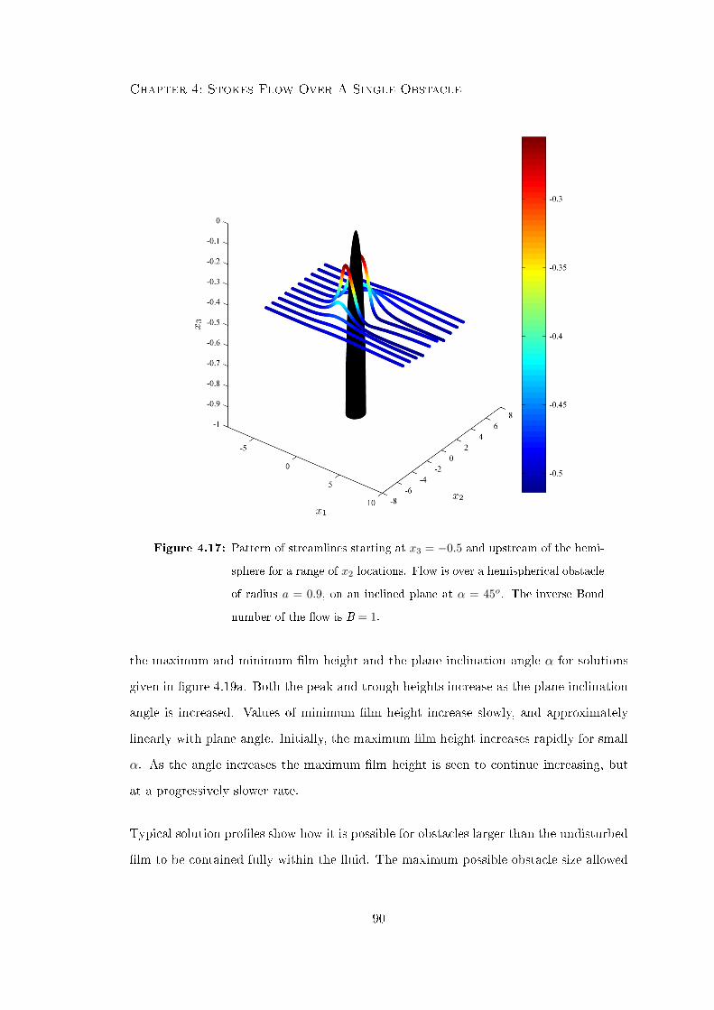
Chapter 4: Stokes Flow Over A Single Obstacle
Figure 4.17: Pattern of streamlines starting at x3 = −0.5 and upstream of the hemi-
sphere for a range of x2 locations. Flow is over a hemispherical obstacle
of radius a = 0.9, on an inclined plane at α = 45o. The inverse Bond
number of the ow is B = 1.
the maximum and minimum lm height and the plane inclination angle α for solutions
given in gure 4.19a. Both the peak and trough heights increase as the plane inclination
angle is increased. Values of minimum lm height increase slowly, and approximately
linearly with plane angle. Initially, the maximum lm height increases rapidly for small
α. As the angle increases the maximum lm height is seen to continue increasing, but
at a progressively slower rate.
Typical solution proles show how it is possible for obstacles larger than the undisturbed
lm to be contained fully within the uid. The maximum possible obstacle size allowed
90
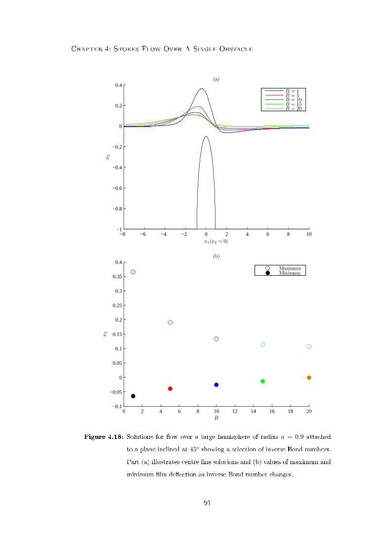
Chapter 4: Stokes Flow Over A Single Obstacle
−8 −6 −4 −2 0 2 4 6 8 10−1
−0.8
−0.6
−0.4
−0.2
0
0.2
0.4(a)
x1(x2 = 0)
x3
0 2 4 6 8 10 12 14 16 18 20−0.1
−0.05
0
0.05
0.1
0.15
0.2
0.25
0.3
0.35
0.4(b)
B
x3
MaximumMinimum
B = 1B = 5B = 10B = 15B = 20
Figure 4.18: Solutions for ow over a large hemisphere of radius a = 0.9 attached
to a plane inclined at 45o showing a selection of inverse Bond numbers.
Part (a) illustrates centre line solutions and (b) values of maximum and
minimum lm deection as inverse Bond number changes.
91
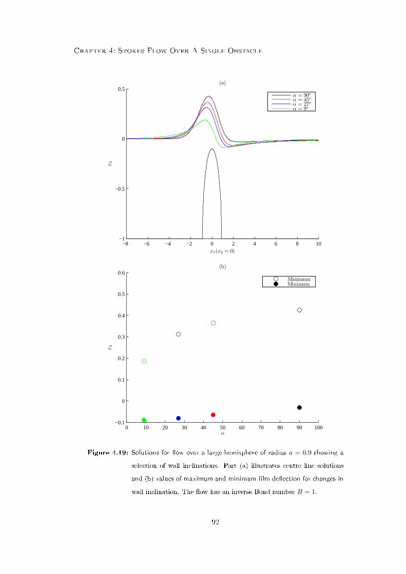
Chapter 4: Stokes Flow Over A Single Obstacle
−8 −6 −4 −2 0 2 4 6 8 10−1
−0.5
0
0.5(a)
x1(x2 = 0)
x3
α = 90o
α = 45o
α = 27o
α = 9o
0 10 20 30 40 50 60 70 80 90 100−0.1
0
0.1
0.2
0.3
0.4
0.5
0.6(b)
α
x3
MaximumMinimum
Figure 4.19: Solutions for ow over a large hemisphere of radius a = 0.9 showing a
selection of wall inclinations. Part (a) illustrates centre line solutions
and (b) values of maximum and minimum lm deection for changes in
wall inclination. The ow has an inverse Bond number B = 1.
92

Chapter 4: Stokes Flow Over A Single Obstacle
within the uid is dependent on the inclination angle of the plane. Two cases are consid-
ered here, ow over large hemispherical obstacles on a shallow plane inclined at 5o and
a steep plane inclined at 90o. For this analysis the hemispheres are discretized by 256
linear triangular elements. A ow domain of −10 ≤ x1 ≤ 10 and −8 ≤ x2 ≤ 8 is taken
with free surface meshes consisting of an element distribution of 40 × 32. Numerical
integration is conducted using the near point singularity approach outlined in § 4.2 and
the zero derivative far eld conditions are again applied within the global RBF analy-
sis. Results are obtained by a simple parameter continuation analysis. A ow prole is
found for an obstacle contained within the uid. The obstacle is then increased in size
(so that it is still within the uid) and the new prole found from the starting point of
the previous solution. This is continued until the obstacle is arbitrarily close to the free
surface.
For ow down a plane inclined at 5o the largest hemispherical obstacle containable within
the Stokes ow has a radius a = 1.028. At this point intersection is imminent on the
back edge of the obstacle where the lm prole collapses towards its trough. A centre
line prole for this obstacle size is shown in gure 4.20a, for a ow with a Bond number
Bo = 1.
For ow down a plane inclined at 90o the largest hemispherical obstacle containable
within the lm ow has a radius of a = 1.92. Interestingly unlike the case for a shallow
plane this limitation is not caused by intersection of the obstacle and free surface, but
rather by limitations on convergence of the model. This may be caused by the ill-
conditioning eects present in the BIE due to the presence of near point singularities.
These eects are more prevalent here than in the shallow plane analysis due to the
extended region of near-point eects. Figure 4.20b illustrates the centre line solutions
for this obstacle on a vertical plane (α = 90o) for ow with a Bond number Bo = 1.
93
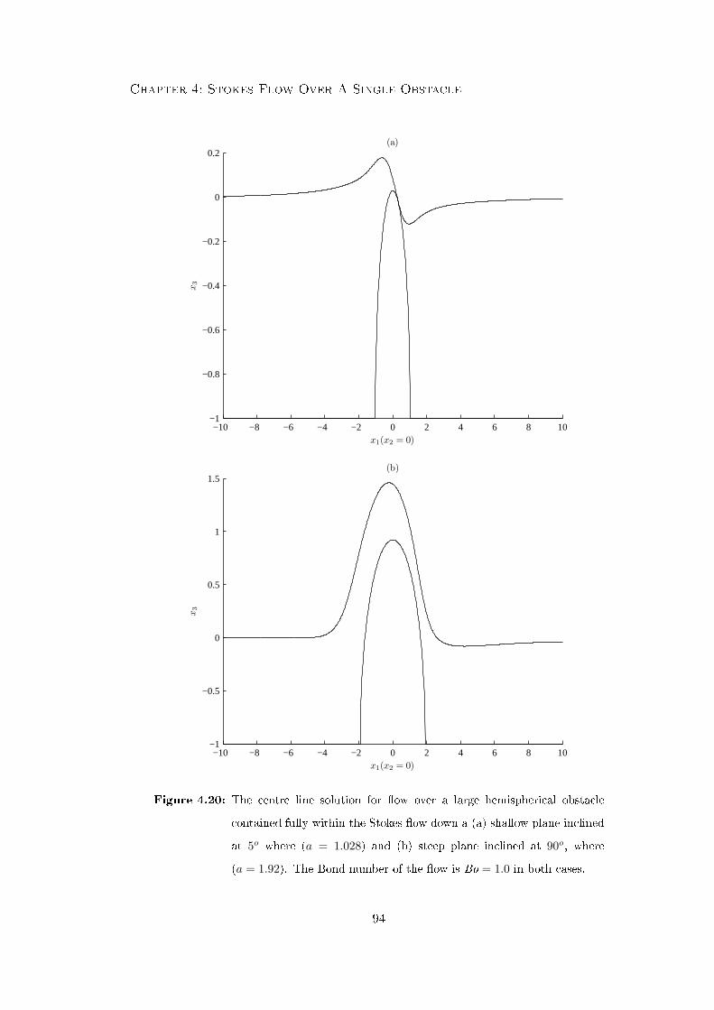
Chapter 4: Stokes Flow Over A Single Obstacle
−10 −8 −6 −4 −2 0 2 4 6 8 10−1
−0.8
−0.6
−0.4
−0.2
0
0.2(a)
x1(x2 = 0)
x3
−10 −8 −6 −4 −2 0 2 4 6 8 10−1
−0.5
0
0.5
1
1.5(b)
x1(x2 = 0)
x3
Figure 4.20: The centre line solution for ow over a large hemispherical obstacle
contained fully within the Stokes ow down a (a) shallow plane inclined
at 5o where (a = 1.028) and (b) steep plane inclined at 90o, where
(a = 1.92). The Bond number of the ow is Bo = 1.0 in both cases.
94
Chapter 5
Stokes Flow Over Multiple
Obstacles
The consideration of Stokes ow over multiple obstacles is a natural extension to the
work outlined in Chapter 4, with § 5.1 modifying the single obstacle formulation to ow
over an arbitrary number of obstacles. The numerical schemes used for solution of the
formulation are identical to those given in § 4.2 using a radial basis function (RBF)
analysis of the full free surface deection. Modication is made to the free surface
mesh, which is developed such that a rened region is present in the location of greatest
deection; details are specied in § 5.2. Solutions corresponding to ow over two and
three hemispheres for a range of relative locations and ow parameters are presented in
§ 5.3.
5.1 Modication To Mathematical Formulation
This section considers the mathematical formulation for a thin lm Stokes ow driven
by gravity down an inclined plane over multiple obstacles attached to the plane. As in §
4.1 the ow variables are solved for disturbance and undisturbed components, yielding
two boundary integral equations (BIEs) for solution over the obstacle and free surface.
95

Chapter 5: Stokes Flow Over Multiple Obstacles
Figure 5.1: Two-dimensional cross section of a typical lm prole over multiple ob-
stacles.
A two-dimensional schematic for ow over N obstacles is shown in gure 5.1, where the
disturbed free surface is denoted Sf and the wall is denoted Sw, and the wetted obstacle
surface of the lth obstacle is denoted Slp. The formulation of the governing equations
follows that presented in § 4.1, although the no slip condition (4.1.6) is modied for each
wetted obstacles surface, i.e.
ui = 0 x ∈ Sw ∪ S1p ∪ S2
p ∪ . . . ∪ SNp , (5.1.1)
uδi = −u∞i x ∈ S1p ∪ S2
p ∪ . . . ∪ SNp . (5.1.2)
The BIE formulation is similar to earlier, except in this case extended to boundaries cor-
responding to multiple obstacles. The Stokes ow equations for the disturbance regime
(equivalent to (4.1.28) for a single obstacle) can be represented exactly as the BIE given
96

Chapter 5: Stokes Flow Over Multiple Obstacles
in (5.1.3) over the uid domain. This gives
cij(x0)uδi (x0) =1
8π
∫Sf∪S1
p∪...∪SNp
G∗ij(x,x0)f δi (x)dS(x)
− 18π
∫Sf∪S1
p∪...∪SNp
uδi (x)T ∗ijk(x,x0)nk(x)dS(x),(5.1.3)
where x is the eld point, and x0 any collocation point and the coecient cij(x0) is given
by (4.1.30). For the N obstacle domains Slp, l = 1, . . . , N the undisturbed quantities
satisfy the N BIEs
cij(x0)u∞i (x0) = − 18π
∫Slp
G∗ij(x,x0)(f∞i (x) +Gni)dS(x)
+1
8π
∫Slp
u∞i (x)T ∗ijk(x,x0)nk(x)dS(x),(5.1.4)
for l = 1, . . . , N , and is equivalent to (4.1.31) for N = 1.
The equivalent BIE to (4.1.34) for collocation over the free surface, is obtained by an
identical procedure to § 4.1, yielding,
12uδj(x0) +
18π
∫Sf
uδi (x)T ∗ijk(x,x0)nk(x)dS(x)
=1
8π
∫S1p∪...∪SNp
G∗ij(x,x0)fi(x)dS(x)
+1
8π
∫Sf
G∗ij(x,x0)f δi (x)dS(x) x0 ∈ Sf .
(5.1.5)
Collocation over a specic wetted obstacle surface x0 ∈ Skp for the BIE (5.1.4) has two
possibilities; BIE (5.1.6) is applicable for l = 1, . . . , k − 1, k + 1, . . . , N ,
18π
∫Slp
G∗ij(x,x0)(f∞i (x) +Gni)dS(x)
=1
8π
∫Slp
u∞i (x)T ∗ijk(x,x0)nk(x)dS(x),(5.1.6)
97
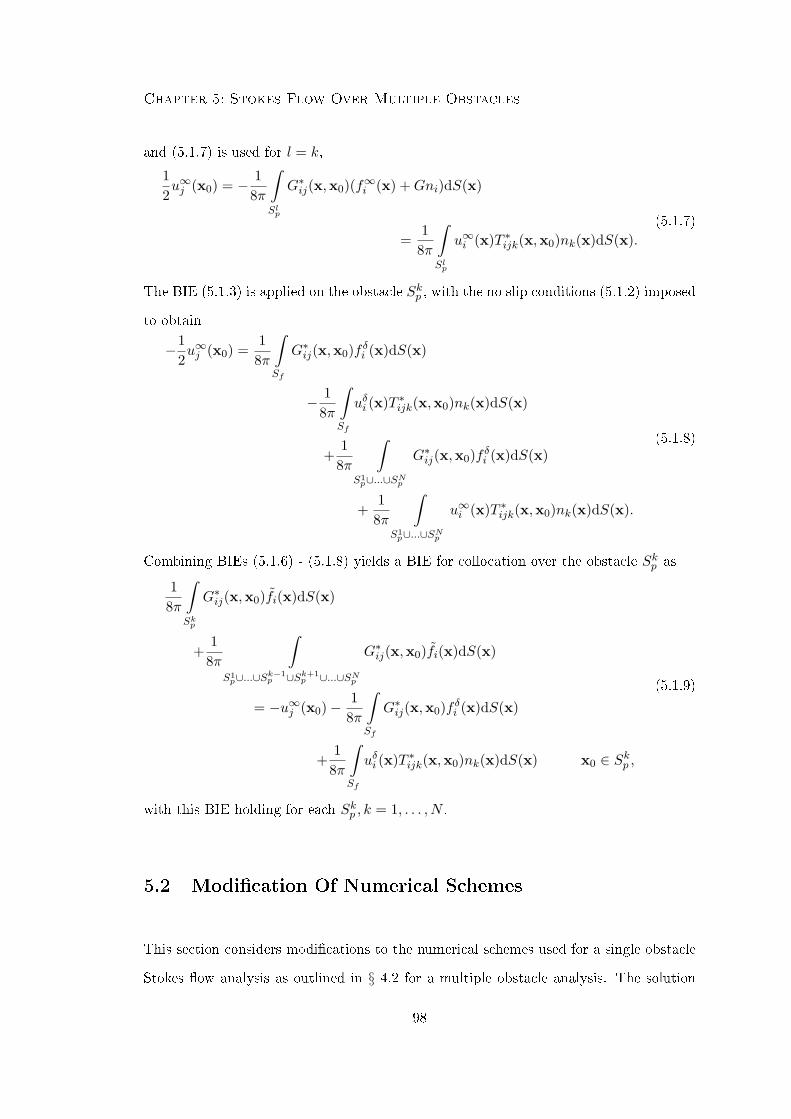
Chapter 5: Stokes Flow Over Multiple Obstacles
and (5.1.7) is used for l = k,
12u∞j (x0) = − 1
8π
∫Slp
G∗ij(x,x0)(f∞i (x) +Gni)dS(x)
=1
8π
∫Slp
u∞i (x)T ∗ijk(x,x0)nk(x)dS(x).(5.1.7)
The BIE (5.1.3) is applied on the obstacle Skp , with the no slip conditions (5.1.2) imposed
to obtain
−12u∞j (x0) =
18π
∫Sf
G∗ij(x,x0)f δi (x)dS(x)
− 18π
∫Sf
uδi (x)T ∗ijk(x,x0)nk(x)dS(x)
+1
8π
∫S1p∪...∪SNp
G∗ij(x,x0)f δi (x)dS(x)
+1
8π
∫S1p∪...∪SNp
u∞i (x)T ∗ijk(x,x0)nk(x)dS(x).
(5.1.8)
Combining BIEs (5.1.6) - (5.1.8) yields a BIE for collocation over the obstacle Skp as
18π
∫Skp
G∗ij(x,x0)fi(x)dS(x)
+1
8π
∫S1p∪...∪S
k−1p ∪Sk+1
p ∪...∪SNp
G∗ij(x,x0)fi(x)dS(x)
= −u∞j (x0)− 18π
∫Sf
G∗ij(x,x0)f δi (x)dS(x)
+1
8π
∫Sf
uδi (x)T ∗ijk(x,x0)nk(x)dS(x) x0 ∈ Skp ,
(5.1.9)
with this BIE holding for each Skp , k = 1, . . . , N .
5.2 Modication Of Numerical Schemes
This section considers modications to the numerical schemes used for a single obstacle
Stokes ow analysis as outlined in § 4.2 for a multiple obstacle analysis. The solution
98
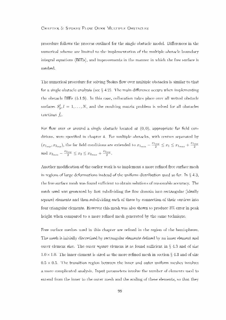
Chapter 5: Stokes Flow Over Multiple Obstacles
procedure follows the process outlined for the single obstacle model. Dierences in the
numerical scheme are limited to the implementation of the multiple obstacle boundary
integral equations (BIEs), and improvements in the manner in which the free surface is
meshed.
The numerical procedure for solving Stokes ow over multiple obstacles is similar to that
for a single obstacle analysis (see § 4.2). The main dierence occurs when implementing
the obstacle BIEs (5.1.9). In this case, collocation takes place over all wetted obstacle
surfaces Slp, l = 1, . . . , N , and the resulting matrix problem is solved for all obstacles
tractions fi.
For ow over or around a single obstacle located at (0, 0), appropriate far eld con-
ditions, were specied in chapter 4. For multiple obstacles, with centres separated by
(x1sep , x2sep), the far eld conditions are extended to x1min −x1sep
2 ≤ x1 ≤ x1max + x1sep
2
and x2min −x2sep
2 ≤ x2 ≤ x2max + x2sep
2 .
Another modication of the earlier work is to implement a more rened free surface mesh
in regions of large deformations instead of the uniform distribution used so far. In § 4.3,
the free surface mesh was found sucient to obtain solutions of reasonable accuracy. The
mesh used was generated by rst subdividing the ow domain into rectangular (ideally
square) elements and then subdividing each of these by connection of their vertices into
four triangular elements. However this mesh was also shown to produce 3% error in peak
height when compared to a more rened mesh generated by the same technique.
Free surface meshes used in this chapter are rened in the region of the hemispheres.
The mesh is initially discretized by rectangular elements dened by an inner element and
outer element size. The outer square element is as found sucient in § 4.3 and of size
1.0×1.0. The inner element is sized as the more rened mesh in section § 4.3 and of size
0.5 × 0.5. The transition region between the inner and outer uniform meshes involves
a more complicated analysis. Input parameters involve the number of elements used to
extend from the inner to the outer mesh and the scaling of these elements, so that they
99
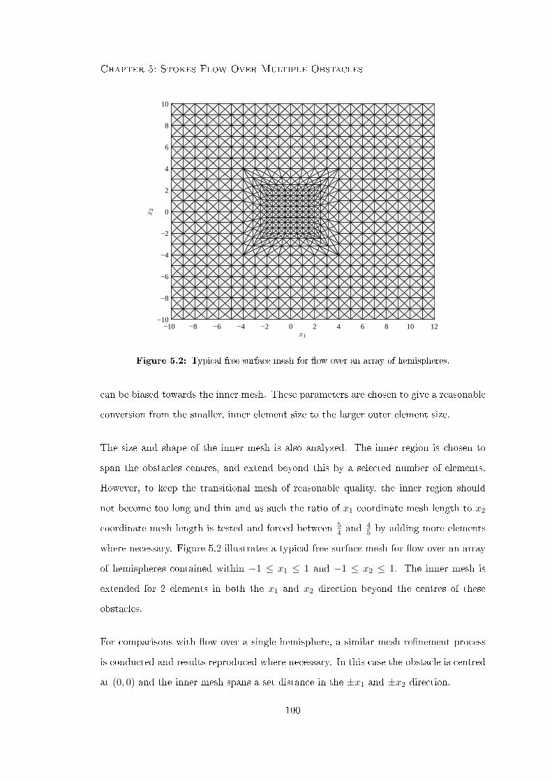
Chapter 5: Stokes Flow Over Multiple Obstacles
−10 −8 −6 −4 −2 0 2 4 6 8 10 12−10
−8
−6
−4
−2
0
2
4
6
8
10
x1
x2
Figure 5.2: Typical free surface mesh for ow over an array of hemispheres.
can be biased towards the inner mesh. These parameters are chosen to give a reasonable
conversion from the smaller, inner element size to the larger outer element size.
The size and shape of the inner mesh is also analyzed. The inner region is chosen to
span the obstacles centres, and extend beyond this by a selected number of elements.
However, to keep the transitional mesh of reasonable quality, the inner region should
not become too long and thin and as such the ratio of x1 coordinate mesh length to x2
coordinate mesh length is tested and forced between 54 and 4
5 by adding more elements
where necessary. Figure 5.2 illustrates a typical free surface mesh for ow over an array
of hemispheres contained within −1 ≤ x1 ≤ 1 and −1 ≤ x2 ≤ 1. The inner mesh is
extended for 2 elements in both the x1 and x2 direction beyond the centres of these
obstacles.
For comparisons with ow over a single hemisphere, a similar mesh renement process
is conducted and results reproduced where necessary. In this case the obstacle is centred
at (0, 0) and the inner mesh spans a set distance in the ±x1 and ±x2 direction.
100
Chapter 5: Stokes Flow Over Multiple Obstacles
5.3 Solution Proles For Flow Over Multiple Obstacles
Flow proles over two and three hemispheres are considered in each of the following
subsections. For ow over two hemispheres, a range of relative obstacle locations are
investigated. For two hemispheres located in-line with the ow direction, a parameter
analysis is considered, where eects of changing the inverse Bond number (4.3.1), plane
inclination angle α, and hemisphere radius a are investigated. Hemispheres of a size that
approach the free surface are also considered, and an analysis is made of how the gap
between the free surface and obstacle is reduced by interaction of a wake on the ow
over a downstream hemisphere.
5.3.1 Solutions For Flow Over Two Hemispheres
Flow over two hemispheres spaced symmetrically to the axis by a distance (x1sep , x2sep)
are considered, with the hemisphere centres located at x1 = ±x1sep
2 and x2 = ±x2sep
2 .
Flow is xed with a Bond number Bo = 1.0 and is down a plane inclined at α = 45o,
with the two attached hemispheres having radius a = 0.9. Flow over a single obstacle
located at (0, 0) required far eld locations −6 ≤ x1 ≤ 8 and −6 ≤ x2 ≤ 6 and for
each dual obstacle analysis the far eld is extended from these values as outlined in the
previous section.
Figure 5.3 illustrates the centre line (x2 = 0) proles of the free surface in the direction of
the upstream ow over two hemispheres in-line with the incident ow and with spacings
x1sep = 2, 4, 6, 8. Dashed proles indicate the equivalent ow over a single hemisphere at
(±x1sep
2 , 0). For all cases of obstacle separation, the deformation caused by the upstream
hemisphere appears to reproduce closely the corresponding prole for a single obstacle.
When the separation is large, the downstream hemisphere of the twin obstacle case
reproduces closely the deformation caused by a single obstacle. This is because the wake
decays after the upstream obstacle and the incident ow conguration to the downstream
101
Chapter 5: Stokes Flow Over Multiple Obstacles
obstacle approximates an undisturbed ow. As the obstacles are moved closer together
the prole over the rear hemisphere is distorted more, with the peak decreasing and the
trough increasing in amplitude. For x1sep ≥ 4, the ow over the rear obstacle appears as
a complete prole, rising from around the undisturbed ow height towards a peak and
decaying behind the obstacle. For x1sep = 2, the prole fundamentally changes, and the
ow over the rear obstacle begins during the collapse of the peak caused by the upstream
obstacle. As such the peaks appear to be joined, with a small step down as ow passes
between obstacles. A single, larger trough is formed downstream of the last obstacle,
instead of behind each hemisphere in turn. This is conrmed by the contour plot in
gure 5.6 for x1sep = 2, x2sep = 0.
Figure 5.4 shows the axis line (x1 = 0) proles of the free surface for ow over two hemi-
spheres spaced perpendicular to the incoming ow direction. Dashed proles correspond
to ow over a single hemisphere at (0,±x2sep
2 ). The obstacle spacing and thus the ow
prole is symmetric in each case about the line x2 = 0. For large separations, the proles
over the two obstacles appear identical to that for a single obstacle. As the obstacles
are moved closer, the outer regions of the ow proles remain consistent with the corre-
sponding single obstacle solution. For x2sep ≥ 4, the inner region of the proles merge,
with the lowest surface point between hemispheres increasing from the undisturbed lm
height. In these cases the peak height above each hemisphere is of similar magnitude
to the single hemisphere case. For x2sep = 2, the two proles merge producing a single
peak, much taller than that created for a single obstacle. The resultant cross-section ow
prole appears as if the ow is interacting with a single larger obstacle. The contour
plot in gure 5.6 for x1sep = 0, x2sep = 2 conrms this.
Figure 5.5 indicates the obstacle and lm surface for the analysis of ow over two hemi-
spheres separated by x1sep = x2sep = 2 and with centres located at (−1,−1) and (1, 1).
The ow is incident to the leading hemisphere, and as the peak splits into a typical
horseshoe shape, one of the raised ridges is incident to the downstream hemisphere.
This thicker lm region causes the peak over the rear hemisphere to be even taller, be-
102
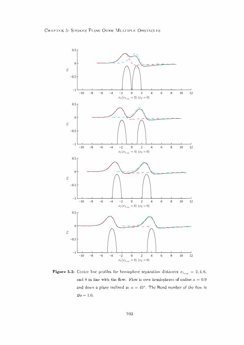
Chapter 5: Stokes Flow Over Multiple Obstacles
−10 −8 −6 −4 −2 0 2 4 6 8 10 12−1
−0.5
0
0.5
x1(x1sep = 2) (x2 = 0)
x3
−10 −8 −6 −4 −2 0 2 4 6 8 10 12−1
−0.5
0
0.5
x1(x1sep = 4) (x2 = 0)
x3
−10 −8 −6 −4 −2 0 2 4 6 8 10 12−1
−0.5
0
0.5
x1(x1sep = 6) (x2 = 0)
x3
−10 −8 −6 −4 −2 0 2 4 6 8 10 12−1
−0.5
0
0.5
x1(x1sep = 8) (x2 = 0)
x3
Figure 5.3: Centre line proles for hemisphere separation distances x1sep= 2, 4, 6,
and 8 in line with the ow. Flow is over hemispheres of radius a = 0.9
and down a plane inclined at α = 45o. The Bond number of the ow is
Bo = 1.0.
103
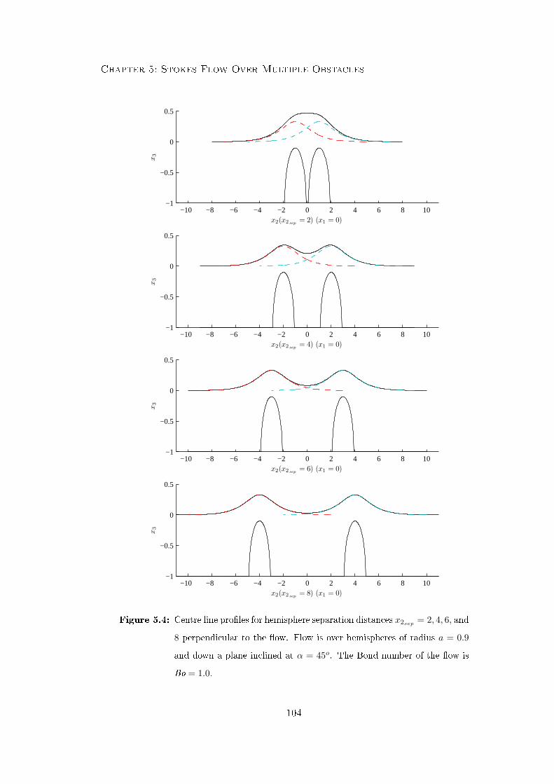
Chapter 5: Stokes Flow Over Multiple Obstacles
−10 −8 −6 −4 −2 0 2 4 6 8 10−1
−0.5
0
0.5
x2(x2sep = 2) (x1 = 0)
x3
−10 −8 −6 −4 −2 0 2 4 6 8 10−1
−0.5
0
0.5
x2(x2sep = 4) (x1 = 0)
x3
−10 −8 −6 −4 −2 0 2 4 6 8 10−1
−0.5
0
0.5
x2(x2sep = 6) (x1 = 0)
x3
−10 −8 −6 −4 −2 0 2 4 6 8 10−1
−0.5
0
0.5
x2(x2sep = 8) (x1 = 0)
x3
Figure 5.4: Centre line proles for hemisphere separation distances x2sep = 2, 4, 6, and
8 perpendicular to the ow. Flow is over hemispheres of radius a = 0.9
and down a plane inclined at α = 45o. The Bond number of the ow is
Bo = 1.0.
104

Chapter 5: Stokes Flow Over Multiple Obstacles
Figure 5.5: Three-dimensional solution prole for two hemispheres of radius a = 0.9,
separated by x1sep= 2, x2sep
= 2. The ow has a Bond number of
Bo = 1.0, and is down a plane inclined at α = 45o
fore decaying in a typical fashion. The close proximity of the two obstacles allows most
of the peaks to merge, with only the tips of the two deections left independent. This is
illustrated further by the contour plot in gure 5.6 for x1sep = 2, x2sep = 2.
Figure 5.6 shows three comparison contour plots for the obstacle congurations corre-
sponding to gures 5.3, 5.4 and 5.5. Clearly, for x1sep = 2, x2sep = 0 the ow is symmetric
in x2 = 0 and the highest point on the free surface occurs just prior to the leading hemi-
sphere. The peak is continued over the rear hemisphere and then collapses rapidly into
a trough around x1 = 1.5. This can also be seen in the centre line plot in gure 5.3. The
contour plot for x1sep = 0, x2sep = 2 again illustrates the symmetry in x2 = 0, with just a
105
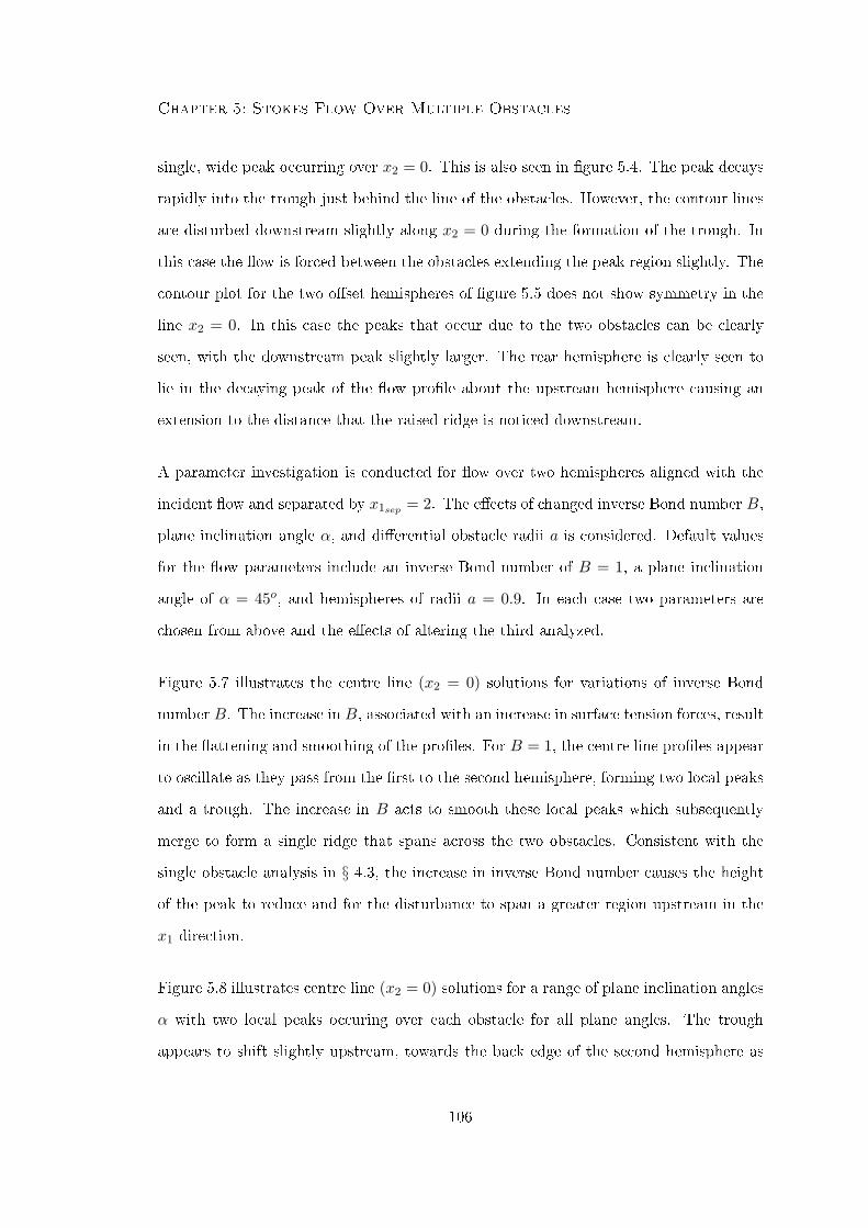
Chapter 5: Stokes Flow Over Multiple Obstacles
single, wide peak occurring over x2 = 0. This is also seen in gure 5.4. The peak decays
rapidly into the trough just behind the line of the obstacles. However, the contour lines
are disturbed downstream slightly along x2 = 0 during the formation of the trough. In
this case the ow is forced between the obstacles extending the peak region slightly. The
contour plot for the two oset hemispheres of gure 5.5 does not show symmetry in the
line x2 = 0. In this case the peaks that occur due to the two obstacles can be clearly
seen, with the downstream peak slightly larger. The rear hemisphere is clearly seen to
lie in the decaying peak of the ow prole about the upstream hemisphere causing an
extension to the distance that the raised ridge is noticed downstream.
A parameter investigation is conducted for ow over two hemispheres aligned with the
incident ow and separated by x1sep = 2. The eects of changed inverse Bond number B,
plane inclination angle α, and dierential obstacle radii a is considered. Default values
for the ow parameters include an inverse Bond number of B = 1, a plane inclination
angle of α = 45o, and hemispheres of radii a = 0.9. In each case two parameters are
chosen from above and the eects of altering the third analyzed.
Figure 5.7 illustrates the centre line (x2 = 0) solutions for variations of inverse Bond
number B. The increase in B, associated with an increase in surface tension forces, result
in the attening and smoothing of the proles. For B = 1, the centre line proles appear
to oscillate as they pass from the rst to the second hemisphere, forming two local peaks
and a trough. The increase in B acts to smooth these local peaks which subsequently
merge to form a single ridge that spans across the two obstacles. Consistent with the
single obstacle analysis in § 4.3, the increase in inverse Bond number causes the height
of the peak to reduce and for the disturbance to span a greater region upstream in the
x1 direction.
Figure 5.8 illustrates centre line (x2 = 0) solutions for a range of plane inclination angles
α with two local peaks occuring over each obstacle for all plane angles. The trough
appears to shift slightly upstream, towards the back edge of the second hemisphere as
106

Chapter 5: Stokes Flow Over Multiple Obstacles
(a)
x1(x1sep = 2)
x2(x
2sep
=0)
−6 −4 −2 0 2 4 6 8−6
−4
−2
0
2
4
6
(b)
x1(x1sep = 0)
x2(x
2sep
=2)
−6 −4 −2 0 2 4 6 8−8
−6
−4
−2
0
2
4
6
8
(c)
x1(x1sep = 2)
x2(x
2sep
=2)
−8 −6 −4 −2 0 2 4 6 8 10−10
−5
0
5
10
−0.1 0 0.1 0.2 0.3 0.4
Figure 5.6: Contour plots for (x1sep , x2sep) = (2, 0), (0, 2), (2, 2). Flow is over two
hemispheres of radius a = 0.9, attached to a plane inclined at α = 45o.
The ow has a Bond number of Bo = 1.0.
107
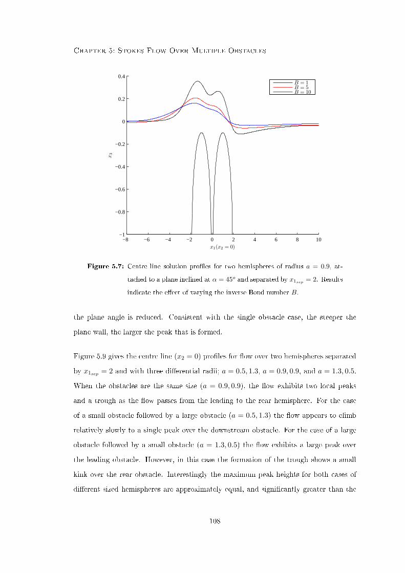
Chapter 5: Stokes Flow Over Multiple Obstacles
−8 −6 −4 −2 0 2 4 6 8 10−1
−0.8
−0.6
−0.4
−0.2
0
0.2
0.4
x1(x2 = 0)
x3
B = 1B = 5B = 10
Figure 5.7: Centre line solution proles for two hemispheres of radius a = 0.9, at-
tached to a plane inclined at α = 45o and separated by x1sep = 2. Results
indicate the eect of varying the inverse Bond number B.
the plane angle is reduced. Consistent with the single obstacle case, the steeper the
plane wall, the larger the peak that is formed.
Figure 5.9 gives the centre line (x2 = 0) proles for ow over two hemispheres separated
by x1sep = 2 and with three dierential radii; a = 0.5, 1.3, a = 0.9, 0.9, and a = 1.3, 0.5.
When the obstacles are the same size (a = 0.9, 0.9), the ow exhibits two local peaks
and a trough as the ow passes from the leading to the rear hemisphere. For the case
of a small obstacle followed by a large obstacle (a = 0.5, 1.3) the ow appears to climb
relatively slowly to a single peak over the downstream obstacle. For the case of a large
obstacle followed by a small obstacle (a = 1.3, 0.5) the ow exhibits a large peak over
the leading obstacle. However, in this case the formation of the trough shows a small
kink over the rear obstacle. Interestingly the maximum peak heights for both cases of
dierent sized hemispheres are approximately equal, and signicantly greater than the
108

Chapter 5: Stokes Flow Over Multiple Obstacles
−8 −6 −4 −2 0 2 4 6 8 10−1
−0.5
0
0.5
x1(x2 = 0)
x3
α = 90o
α = 45o
α = 27o
α = 9o
Figure 5.8: Centre line solution proles for two hemispheres of radius a = 0.9 sep-
arated by x1sep = 2, showing the eect of varying the plane inclination
angle α. The ow has an inverse Bond number of B = 1.0.
Shallow (α = 5o) plane with a = 1.05 Steep (α = 90o) plane with a = 1.60
Single 0.0486 0.337
Double 0.0465 0.220
Table 5.1: Near point values (3.s.f.) for large hemispheres on shallow and steep planes.
case of equal hemisphere size; this suggests the peak height is strongly dependent on
the maximum hemisphere radius. The corresponding lm height for ow over a single
hemisphere of radius a = 1.3 is provided allowing comparison with the dual hemisphere
solutions. When the large hemisphere precedes the small hemisphere, ow over this
obstacle shows negligible discrepancy to the single case. When the large hemisphere is
the rear obstacle, a small dierence to the single obstacle solution is present.
In § 4.3 it was found that the largest possible hemisphere containable within the uid lm
was strongly dependent on the inclination of the plane. Proles have been compared for
109
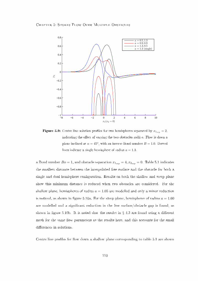
Chapter 5: Stokes Flow Over Multiple Obstacles
−8 −6 −4 −2 0 2 4 6 8 10−1
−0.8
−0.6
−0.4
−0.2
0
0.2
0.4
0.6
0.8
x1(x2 = 0)
x3
a = 0.5, 1.3a = 0.9, 0.9a = 1.3, 0.5a = 1.3 (single)
Figure 5.9: Centre line solution proles for two hemispheres separated by x1sep= 2,
indicating the eect of varying the two obstacles radii a. Flow is down a
plane inclined at α = 45o, with an inverse Bond number B = 1.0. Dotted
lines indicate a single hemisphere of radius a = 1.3.
a Bond number Bo = 1, and obstacle separation x1sep = 4, x2sep = 0. Table 5.1 indicates
the smallest distance between the interpolated free surface and the obstacle for both a
single and dual hemisphere conguration. Results on both the shallow and steep plane
show this minimum distance is reduced when two obstacles are considered. For the
shallow plane, hemispheres of radius a = 1.05 are modelled and only a minor reduction
is noticed, as shown in gure 5.10a. For the steep plane, hemispheres of radius a = 1.60
are modelled and a signicant reduction in the free surface/obstacle gap is found, as
shown in gure 5.10b. It is noted that the results in § 4.3 are found using a dierent
mesh for the same ow parameters as the results here, and this accounts for the small
dierences in solutions.
Centre line proles for ow down a shallow plane corresponding to table 5.1 are shown
110

Chapter 5: Stokes Flow Over Multiple Obstacles
−10 −8 −6 −4 −2 0 2 4 6 8 10 12−1
−0.8
−0.6
−0.4
−0.2
0
0.2(a)
x1(x2 = 0)
x3
−10 −8 −6 −4 −2 0 2 4 6 8 10 12−1
−0.8
−0.6
−0.4
−0.2
0
0.2
0.4
0.6
0.8
1
(b)
x1(x2 = 0)
x3
Figure 5.10: Centre line solution for ow over large hemispheres of radius (a) a = 1.05
attached to a shallow plane at α = 5o (b) a = 1.60 attached to a steep
plane at α = 90o. The Bond number of the ow in both cases is Bo = 1.0.
Comparison is shown with a single hemisphere for both gures.
111

Chapter 5: Stokes Flow Over Multiple Obstacles
Figure 5.11: Three-dimensional solution prole for three hemispheres located at
(−2,−2), (−2, 2), (2, 0). The ow has a Bond number of Bo = 1.0,
is down a plane inclined at α = 45o, and the hemispheres each have a
radius of a = 0.9.
in gure 5.10a. Flow is down a plane inclined at α = 5o, and a minor reduction in the
gap between the obstacle and free surface is found behind the rear hemisphere when
compared with a single obstacle analysis. Centre line solutions for ow down a steep
plane corresponding to the information in table 5.1 are shown in gure 5.10b. Flow is
down a plane inclined at α = 90o, and a signicant reduction in the near point values
between the obstacle and free surface is found behind the rear hemispherical obstacle
when compared with a single obstacle analysis.
112

Chapter 5: Stokes Flow Over Multiple Obstacles
Figure 5.12: Three-dimensional solution prole for three hemispheres located at
(−2, 0), (2,−2), (2, 2). The ow has a Bond number of Bo = 1.0, is
down a plane inclined at α = 45o, and the hemispheres each have a
radius of a = 0.9.
5.3.2 Solutions For Flow Over Three Hemispheres
Illustration of ow over three hemispheres is now given for two obstacle congurations.
Flow has a Bond number Bo = 1, all hemispheres have a radius of a = 0.9 and the
plane is inclined at α = 45o. Obstacles are positioned in a symmetrical triangular array,
with either a twin or single leading hemisphere conguration considered. A twin leading
conguration is illustrated in gure 5.11 and consists of the upstream ow incident on
two obstacles spaced perpendicularly to the ow direction with centres (−2,−2), (−2, 2).
This is followed by a trailing hemisphere centered at (2, 0). The conguration shown in
113
Chapter 5: Stokes Flow Over Multiple Obstacles
gure 5.12 consists of the upstream ow incident on one obstacle centered at (−2, 0)
followed by two downstream hemispheres spaced perpendicularly to the ow direction
with centres at (2,−2), (2, 2). In both cases, three peaks are clearly seen just prior to
each obstacle.
114
Chapter 6
Stokes Flow Around Obstacles
Flow proles for thin lm Stokes ow down an inclined plane over multiple obstacles
in a range of congurations are considered. When these obstacles are increased in size
they will eventually penetrate the lm surface, leading to lm ows around obstacles
and adding another layer of complexity to the model. A contact angle constraint is
imposed at the contact line within the radial basis function (RBF) interpolation, and the
boundary integral equation (BIE) over the obstacle domain requires closing by addition
of a top to the obstacle. Further details of the mathematical formulation are given in
§ 6.1. In addition, the obstacle requires re-meshing at each iteration, and a mesh must
be generated for the top of the obstacle. Details of the numerical schemes implemented
are given in § 6.2. Solution proles for ow around single and multiple obstacles are
produced in § 6.3, and the possibility of multiple solutions examined. These occur when
a ow with xed parameters may pass over or around an obstacle, and the resultant
prole is dependent on the initial conditions. Multiple solutions are also examined in
the case of two obstacles, to consider ow over then around an identical obstacle. All
results shown in this chapter are for circular cylinders.
115
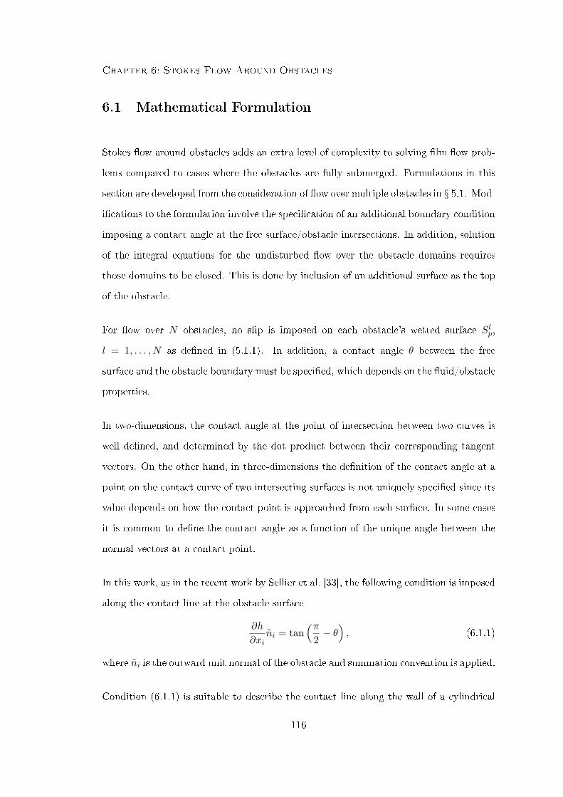
Chapter 6: Stokes Flow Around Obstacles
6.1 Mathematical Formulation
Stokes ow around obstacles adds an extra level of complexity to solving lm ow prob-
lems compared to cases where the obstacles are fully submerged. Formulations in this
section are developed from the consideration of ow over multiple obstacles in § 5.1. Mod-
ications to the formulation involve the specication of an additional boundary condition
imposing a contact angle at the free surface/obstacle intersections. In addition, solution
of the integral equations for the undisturbed ow over the obstacle domains requires
those domains to be closed. This is done by inclusion of an additional surface as the top
of the obstacle.
For ow over N obstacles, no slip is imposed on each obstacle's wetted surface Slp,
l = 1, . . . , N as dened in (5.1.1). In addition, a contact angle θ between the free
surface and the obstacle boundary must be specied, which depends on the uid/obstacle
properties.
In two-dimensions, the contact angle at the point of intersection between two curves is
well dened, and determined by the dot product between their corresponding tangent
vectors. On the other hand, in three-dimensions the denition of the contact angle at a
point on the contact curve of two intersecting surfaces is not uniquely specied since its
value depends on how the contact point is approached from each surface. In some cases
it is common to dene the contact angle as a function of the unique angle between the
normal vectors at a contact point.
In this work, as in the recent work by Sellier et al. [33], the following condition is imposed
along the contact line at the obstacle surface
∂h
∂xini = tan
(π2− θ), (6.1.1)
where ni is the outward unit normal of the obstacle and summation convention is applied.
Condition (6.1.1) is suitable to describe the contact line along the wall of a cylindrical
116

Chapter 6: Stokes Flow Around Obstacles
Figure 6.1: Schematic showing the two-dimensional denition of the contact angle.
obstacle with constant cross section, and located perpendicular to the undisturbed lm
prole, i.e. n3 = 0. This condition is an extension to three-dimensions of the two-
dimensional denition of the contact angle between a free surface and vertical wall, where
the slope of the curve describing the free surface at the contact point is dhdx1
= tan(α) =
cot(θ), and α = π2 − θ. The dot product of the normal vectors is cos(ϕ) = cos(π − θ) =
− dhdx1
/
√(dhdx1
)2+ 1, where the angle between the normal vectors is ϕ = π
2 + α, and
therefore sin(ϕ) = 1/
√(dhdx1
)2+ 1. A schematic for the two-dimensional denition of
the contact angle condition is shown in gure 6.1. Consequently, equation (6.1.1) gives
the slope of the curve dened by the intersection between a normal plane to the cylinder,
εijknjδk3, and the free surface, at a contact point along the cylinder wall, i.e. the contact
angle is a measure from the cylindrical wall to the free surface along a normal plane to
the cylinder wall.
For ow around an obstacle, the integral formulation remains largely unchanged, but
two additional terms are present in the boundary integral equations (BIEs). Figure 6.2
indicates a schematic of the nomenclature used for ow around a cylinder. The free
surface is still labeled Sf along with the wetted obstacle surfaces Slp l = 1, . . . , N . The
obstacle domain is no longer closed solely by the wall Sw and the wetted obstacle surfaces
117
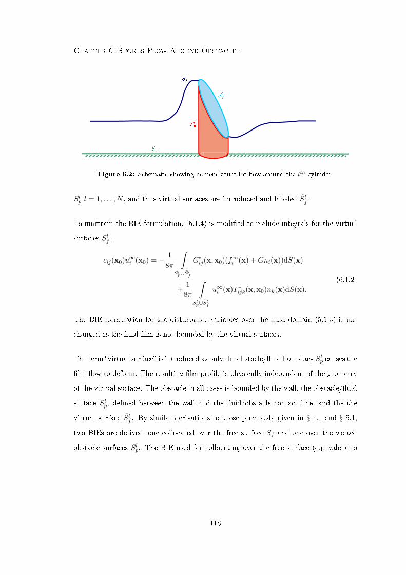
Chapter 6: Stokes Flow Around Obstacles
Figure 6.2: Schematic showing nomenclature for ow around the lth cylinder.
Slp l = 1, . . . , N , and thus virtual surfaces are introduced and labeled Slf .
To maintain the BIE formulation, (5.1.4) is modied to include integrals for the virtual
surfaces Slf ,
cij(x0)u∞i (x0) = − 18π
∫Slp∪Slf
G∗ij(x,x0)(f∞i (x) +Gni(x))dS(x)
+1
8π
∫Slp∪Slf
u∞i (x)T ∗ijk(x,x0)nk(x)dS(x).(6.1.2)
The BIE formulation for the disturbance variables over the uid domain (5.1.3) is un-
changed as the uid lm is not bounded by the virtual surfaces.
The term virtual surface is introduced as only the obstacle/uid boundary Slp causes the
lm ow to deform. The resulting lm prole is physically independent of the geometry
of the virtual surface. The obstacle in all cases is bounded by the wall, the obstacle/uid
surface Slp, dened between the wall and the uid/obstacle contact line, and the the
virtual surface Slf . By similar derivations to those previously given in § 4.1 and § 5.1,
two BIEs are derived, one collocated over the free surface Sf and one over the wetted
obstacle surfaces Slp. The BIE used for collocating over the free surface (equivalent to
118
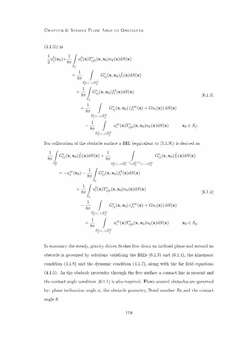
Chapter 6: Stokes Flow Around Obstacles
(5.1.5)) is
12uδj(x0)+
18π
∫Sf
uδi (x)T ∗ijk(x,x0)nk(x)dS(x)
=1
8π
∫S1p∪...∪SNp
G∗ij(x,x0)fi(x)dS(x)
+1
8π
∫Sf
G∗ij(x,x0)f δi (x)dS(x)
+1
8π
∫S1f∪...∪S
Nf
G∗ij(x,x0) (f∞i (x) +Gni(x)) dS(x)
− 18π
∫S1f∪...∪S
Nf
u∞i (x)T ∗ijk(x,x0)nk(x)dS(x) x0 ∈ Sf .
(6.1.3)
For collocation of the obstacle surface a BIE (equivalent to (5.1.9)) is derived as
18π
∫Skp
G∗ij(x,x0)fi(x)dS(x) +1
8π
∫S1p∪...∪S
k−1p ∪Sk+1
p ∪...∪SNp
G∗ij(x,x0)fi(x)dS(x)
= −u∞j (x0)− 18π
∫Sf
G∗ij(x,x0)f δi (x)dS(x)
+1
8π
∫Sf
uδi (x)T ∗ijk(x,x0)nk(x)dS(x)
− 18π
∫S1f∪...∪S
Nf
G∗ij(x,x0) (f∞i (x) +Gni(x)) dS(x)
+1
8π
∫S1f∪...∪S
Nf
u∞i (x)T ∗ijk(x,x0)nk(x)dS(x) x0 ∈ Sp.
(6.1.4)
In summary the steady, gravity driven Stokes ow down an inclined plane and around an
obstacle is governed by solutions satisfying the BIEs (6.1.3) and (6.1.4), the kinematic
condition (4.1.8) and the dynamic condition (4.1.7), along with the far eld equations
(4.1.5). As the obstacle protrudes through the free surface a contact line is present and
the contact angle condition (6.1.1) is also required. Flows around obstacles are governed
by: plane inclination angle α, the obstacle geometry, Bond number Bo and the contact
angle θ.
119

Chapter 6: Stokes Flow Around Obstacles
6.2 Numerical Schemes
This section considers modications to the numerical schemes used for a multiple ob-
stacle Stokes ow analysis as outlined in § 5.2 for lm ows around multiple obstacles.
Developments in the numerical schemes involve meshing the circular cylindrical obsta-
cles and free surface, along with incorporation of the contact angle constraint within
the RBF interpolation of the free surface. Both of these are detailed later in respective
subsections.
The iterative procedure for nding solutions to ow around multiple obstacles diers
from that outlined for ow over an obstacle in § 4.2. The procedure used to obtain
solutions in the present case of ow around multiple obstacles is dened below, with the
unknown integral densities uδi on Sf , and fi on S1p ∪ . . . ∪ SNp obtained.
(i) Initially at the free surface elements mid-points xm = (xm1 , xm2 ), a lm prole is
dened by heights h with corresponding disturbance velocities uδi .
(ii) The free surface heights h are interpolated using a radial basis function (RBF),
incorporating the far eld and contact angle condition, and used to nd:
(a) the heights at the nodal points of each free surface element xn = (xn1 , xn2 );
(b) the outward unit normal of the free surface at the element mid-points, xm;
(c) the curvature of the free surface at the element mid-points, xm.
(iii) The contact line is found, and the wetted obstacle surface Slp is meshed from the
wall Sw to the contact line. In addition a mesh for the top of the obstacle Slf is
also generated.
(iv) The disturbance boundary traction at the free surface element mid-points xm is
calculated by use of the dynamic condition (4.1.27).
(v) The obstacle boundary integral equations (BIEs) (6.1.4) are collocated over all
120
Chapter 6: Stokes Flow Around Obstacles
obstacles/uid surfaces Skp , k = 1, . . . , N for tractions fi. Solutions are obtained by
using the boundary element method (BEM).
(vi) The free surface BIE (6.1.3) is collocated over Sf for the free surface disturbance
velocities at each elements mid-points. It is noted that the height of the element
mid-points are approximated within this BEM formulation by the average of the
nodal point heights.
(vii) The kinematic condition (4.1.8) is applied with the current values of h and the
calculated values of uδi at element mid-points xm, to nd an updated set of h
dening the free surface.
(viii) The process is repeated from step 2 using the new lm prole.
As outlined in chapter 4 for ow over an obstacle, the only place that the free surface
height is approximated within the iterative solution procedure is for collocation over
the free surface within the BEM. In all other calculations, the height at any mid ele-
ment location is associated with the interpolated surface. This limitation is caused by
implementing at triangular elements within the BEM.
The numerical schemes required to solve the problem are now discussed. This includes
forms for the meshes used for the free surface, and obstacle (including the wetted sur-
face and the top of the obstacle), and the implementation of the RBF to evaluate the
free surface position and various quantities such as curvature and unit normal, whilst
constraining the contact angle (6.1.1). The BEM and near point integration schemes are
implemented as described in § 4.2
6.2.1 Surface Discretizations
The obstacle/uid boundaries, free surface, and virtual obstacle tops all require dis-
cretization. Circular cylinders are modelled throughout, satisfying the contact angle
121
Chapter 6: Stokes Flow Around Obstacles
constraint (6.1.1).
For circular cylindrical obstacles, the top edge of the cylinder was rst considered with
the circular perimeter of the cylinder discretized by a polygon of specied resolution and
vertical lines subtended down its sides. In addition the height of the cylinder at each
polygonal vertex was split evenly into a number of slices. The intersections of these
two divisions form rectangular elements which were subdivided again into 4 triangular
elements by connection of the diagonal vertices. Illustration of typical meshes for cylin-
drical cylinders are shown in gure 6.3. In cases for ow over and around a circular
cylinder a form for the mesh on the top surface is required. The x1x2 element distri-
bution of the top of the cylinder is generated by successive subdivision. This is slightly
more complicated than the case of a hemisphere as it is only the outermost element sides
that require translating onto the edge of the circle at each subdivision. At the end of the
subdivision process the vertical position is dened depending on the case analyzed. For
ow over a cylinder, each node is translated onto the sloped top of the cylinder, dened
by its height at the upstream location x1 = −a and the downstream location x1 = a.
The height varies linearly in the x1 direction between these two points. An example
mesh for the cylinder in this case is shown in gure 6.3a. For ow around a cylinder, the
top is dened by a RBF interpolation that also holds the normal gradients as zero on the
outer edge of the cylinder. The functional values that require evaluation on the surface
Sf are calculated using an inward pointing normal as dened by the RBF interpolation.
An example mesh for a cylinder with an interpolated top is shown in gure 6.3b.
Free surface meshes are modied from the earlier work considering ow over obstacles
to allow the obstacle to penetrate the free surface. Formation of the meshes for both a
single and multiple cylinder array is discussed below. In the case of a single cylinder the
mesh is formed in a similar fashion to that outlined for the rened multiple hemisphere
analysis in § 5.2. However, in the present case, there is no inner mesh and the transitional
mesh is instead used to t the discretized prole for the cylinder's contact line to the
outer mesh. Again the outer mesh is constructed from elements of the size 1.0× 1.0 as
122

Chapter 6: Stokes Flow Around Obstacles
−10
1 −1
0
1−1
−0.8
−0.6
−0.4
−0.2
0
0.2
0.4
x2x1
x3
−1
0
1 −1
0
1−1
−0.8
−0.6
−0.4
−0.2
0
0.2
0.4
0.6
0.8
1
x2x1
x3
(a) (b)
Figure 6.3: Typical mesh for a cylindrical obstacle, with (a) a truncated top and (b)
an interpolated top.
found sucient in earlier analysis. In each case the transitional mesh is formed by the
input parameters of the number of elements used to extend from the cylinder wall to the
outer mesh and the scaling of these elements. The choice of these parameters is made to
give a reasonable conversion from the smaller, cylinder element size to the larger outer
element size. A typical free surface mesh is shown in gure 6.4.
Free surface meshes for ow around multiple cylinders use alternative methods depending
on the separation distance between the cylinders. If the cylinders are suciently far apart
the mesh is formed by identical means to that outlined above, tting the transitional
meshes locally within the global outer mesh. However, if the transition meshes from
each cylinder to the outer mesh overlap, then modication of this technique is required.
An intermediate mesh with smaller element size than the outer mesh is dened. The
cylinders are tted to the intermediate mesh, and the intermediate mesh is then extended
to the outer mesh in a similar way to the mesh formation for multiple hemispheres. Figure
6.5 indicates a typical free surface mesh for the case where ow is around 3 cylinders
123

Chapter 6: Stokes Flow Around Obstacles
−8 −6 −4 −2 0 2 4 6 8 10 12−8
−6
−4
−2
0
2
4
6
8
x1
x2
Figure 6.4: Typical free surface mesh for ow around a single cylinder of radius a =
1.0.
close to one another.
6.2.2 Radial Basis Function For Flow Around Cylinders
As for the case of ow over obstacles, a global Hermitian RBF interpolation of the uid
free surface is implemented. The RBF ψ(‖x − ξ‖) allows incorporation of the far eld
derivative conditions and also the contact line condition for each obstacle that penetrates
the free surface. As before the surface is interpolated using a thin plate spline RBF of the
form ψ = r4 log r, where r = ‖x− ξ‖, and is chosen to remove singularities of ψ at r = 0
for up to and including its third derivative. To guarantee invertibility, an additional
polynomial of order 2 is required along with a homogeneous constraint condition.
The RBF can be used to constrain the free surface gradient at n far eld points and ncl
contact line points. Surface displacements and derivatives ∂h∂x1
and ∂h∂x2
are represented
124
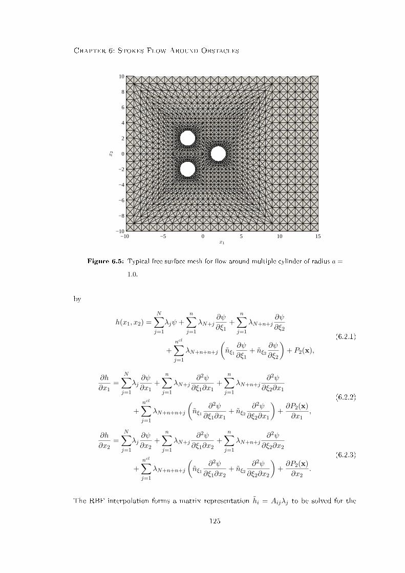
Chapter 6: Stokes Flow Around Obstacles
−10 −5 0 5 10 15−10
−8
−6
−4
−2
0
2
4
6
8
10
x1
x2
Figure 6.5: Typical free surface mesh for ow around multiple cylinder of radius a =
1.0.
by
h(x1, x2) =N∑j=1
λjψ +n∑j=1
λN+j∂ψ
∂ξ1+
n∑j=1
λN+n+j∂ψ
∂ξ2
+ncl∑j=1
λN+n+n+j
(nξ1
∂ψ
∂ξ1+ nξ2
∂ψ
∂ξ2
)+ P2(x),
(6.2.1)
∂h
∂x1=
N∑j=1
λj∂ψ
∂x1+
n∑j=1
λN+j∂2ψ
∂ξ1∂x1+
n∑j=1
λN+n+j∂2ψ
∂ξ2∂x1
+ncl∑j=1
λN+n+n+j
(nξ1
∂2ψ
∂ξ1∂x1+ nξ2
∂2ψ
∂ξ2∂x1
)+∂P2(x)∂x1
,
(6.2.2)
∂h
∂x2=
N∑j=1
λj∂ψ
∂x2+
n∑j=1
λN+j∂2ψ
∂ξ1∂x2+
n∑j=1
λN+n+j∂2ψ
∂ξ2∂x2
+ncl∑j=1
λN+n+n+j
(nξ1
∂2ψ
∂ξ1∂x2+ nξ2
∂2ψ
∂ξ2∂x2
)+∂P2(x)∂x2
.
(6.2.3)
The RBF interpolation forms a matrix representation hi = Aijλj to be solved for the
125
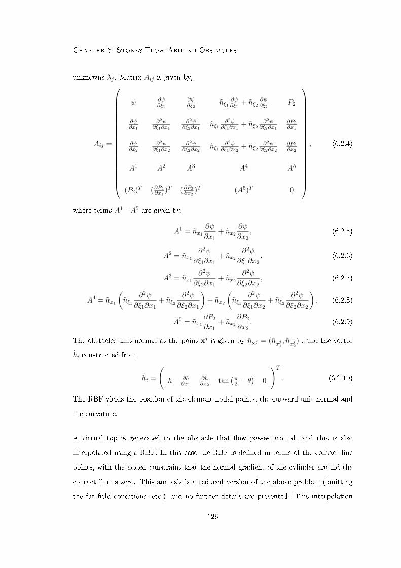
Chapter 6: Stokes Flow Around Obstacles
unknowns λj . Matrix Aij is given by,
Aij =
ψ ∂ψ∂ξ1
∂ψ∂ξ2
nξ1∂ψ∂ξ1
+ nξ2∂ψ∂ξ2
P2
∂ψ∂x1
∂2ψ∂ξ1∂x1
∂2ψ∂ξ2∂x1
nξ1∂2ψ
∂ξ1∂x1+ nξ2
∂2ψ∂ξ2∂x1
∂P2∂x1
∂ψ∂x2
∂2ψ∂ξ1∂x2
∂2ψ∂ξ2∂x2
nξ1∂2ψ
∂ξ1∂x2+ nξ2
∂2ψ∂ξ2∂x2
∂P2∂x2
A1 A2 A3 A4 A5
(P2)T (∂P2∂x1
)T (∂P2∂x2
)T (A5)T 0
, (6.2.4)
where terms A1 - A5 are given by,
A1 = nx1
∂ψ
∂x1+ nx2
∂ψ
∂x2, (6.2.5)
A2 = nx1
∂2ψ
∂ξ1∂x1+ nx2
∂2ψ
∂ξ1∂x2, (6.2.6)
A3 = nx1
∂2ψ
∂ξ2∂x1+ nx2
∂2ψ
∂ξ2∂x2, (6.2.7)
A4 = nx1
(nξ1
∂2ψ
∂ξ1∂x1+ nξ2
∂2ψ
∂ξ2∂x1
)+ nx2
(nξ1
∂2ψ
∂ξ1∂x2+ nξ2
∂2ψ
∂ξ2∂x2
), (6.2.8)
A5 = nx1
∂P2
∂x1+ nx2
∂P2
∂x2. (6.2.9)
The obstacles unit normal at the point xj is given by nxj = (nxj1, n
xj2) , and the vector
hi constructed from,
hi =
(h ∂h
∂x1
∂h∂x2
tan(π2 − θ
)0
)T. (6.2.10)
The RBF yields the position of the element nodal points, the outward unit normal and
the curvature.
A virtual top is generated to the obstacle that ow passes around, and this is also
interpolated using a RBF. In this case the RBF is dened in terms of the contact line
points, with the added constraint that the normal gradient of the cylinder around the
contact line is zero. This analysis is a reduced version of the above problem (omitting
the far eld conditions, etc.) and no further details are presented. This interpolation
126

Chapter 6: Stokes Flow Around Obstacles
allows the inward unit normal to be found, necessary for evaluating the traction values
on this surface, as used in BIEs (6.1.3) and (6.1.4).
6.3 Solution Proles For Flow Around Obstacles
In this section results for ow around cylindrical obstacles on an inclined plane are
presented. Results are initially shown for ow around a single cylinder on an inclined
plane, with the possibility of solutions where both ow around and ow over an obstacle is
valid, satisfying all requirements and demonstrating the possibilities of multiple solutions.
Results for ow around multiple cylinders, and also the possibility of ow over, then
around identical cylinders spaced in the direction of the incoming ow are presented.
6.3.1 Solutions For Flow Around Single Obstacles
Before results are produced, a mesh analysis was conducted on a free surface in the
domain −8 ≤ x1 ≤ 10 and −8 ≤ x2 ≤ 8. The outer free surface mesh was based
on 1.0 × 1.0 elements, found to be sucient to describe large free surface deformations
in chapter 4. Mesh considerations involve the number of vertical discretizations of the
cylinder wall, and the resolution of the transitional mesh of the free surface connecting
the cylinder to the outer meshes.
The obstacle discretization is governed by two key parameters, the circumferential dis-
cretization and the vertical discretization. Circumferentially, the cylinder is discretized
32 times, identical to that found optimal for the base of a hemisphere in earlier sections.
Vertically, the cylinder was discretized into segments and proles changed nominally
with selection. Five vertical discretizations are used for the cylinder mesh, producing
solutions which appear invariant to further renement, and also helping to maintain the
regularity of the mesh when large displacements are found between the upstream and
127

Chapter 6: Stokes Flow Around Obstacles
−1.5 −1 −0.5 00.2
0.25
0.3
0.35
0.4
0.45
x1(x2 = 0)
x3
UnrefinedSatisfactoryRefinedVery Refined
Figure 6.6: Centre line solution at the upstream edge of the cylinder indicating the
transitional mesh resolutions described in table 6.1 for ow around a
cylinder of radius a = 0.5.
downstream contact position on the obstacle.
The transitional mesh of the free surface involves a more complicated analysis. Input
parameters involve the number of elements used to extend from the cylinder wall to
the outer mesh and the scaling of these elements, so that they can be biased towards
the cylinder wall. Four cases were considered with the number of elements and scaling
values for each analysis shown in table 6.1. Solutions for these four transitional mesh
resolutions are shown in gure 6.6.
All transitional mesh regimes are found to give accurate portrayals of the global ow
prole. However, the eects of the contact line condition on the ow prole local to
the cylinder is marginally aected by the transitional mesh resolutions used, especially
for the case of an unrened transitional discretization. As the mesh is progressively
rened the solutions tend towards a converged solution. However, it is found that use of
128

Chapter 6: Stokes Flow Around Obstacles
Number of Elements Transitional Element Scaling Factor
Unrened 4 0.60
Satisfactory 5 0.60
Rened 6 0.65
Very Rened 7 0.70
Table 6.1: Transitional free surface mesh regimes.
the rened mesh (see table 6.1 and gure 6.6) is adequate to accurately represent the
ow regime around the cylinder and it is this transitional mesh resolution that is used
throughout for cylinders of radius a = 0.5. For larger cylinders, the transitional mesh
is changed but each time analyzed to maintain a similar resolution of elements as found
sucient for the a = 0.5 case considered here. For some results, the far eld is extended
to help maintain convergence and sucient decay of the free surface disturbance.
Figure 6.7 shows the full free surface for ow around a cylinder of radius a = 2.0. The
ow was down a plane inclined at α = 45o and the lm has a Bond number Bo = 0.89
corresponding to an inverse Bond number of 1 as dened in (4.3.1) and used by Blyth
and Pozrikidis [31]. The contact angle at the cylinder walls was constrained to θ = 90o.
A typical obstacle mesh can be seen in gure 6.3.
Figure 6.8 shows the streamlines for ow around a circular cylinder attached to a plane
inclined at 45o. The cylinder has a radius of a = 0.5 with a contact angle condition of
θ = 90o specied on the cylinder wall. The ow has an inverse Bond number of B = 1.
Streamlines close to the cylinder are deected upwards, as well as around the cylinder.
In addition, as with the lm proles, solutions show symmetry about the plane x2 = 0.
Figure 6.9a illustrates solutions for a range of inverse Bond numbers B. Flow is down
a plane inclined at α = 45o around a cylindrical obstacle of radius a = 0.5. The free
surface/obstacle interface was modelled by a contact angle of θ = 90o. Increasing the
inverse Bond number (i.e. raising the ratio of surface tension forces to gravitational
129
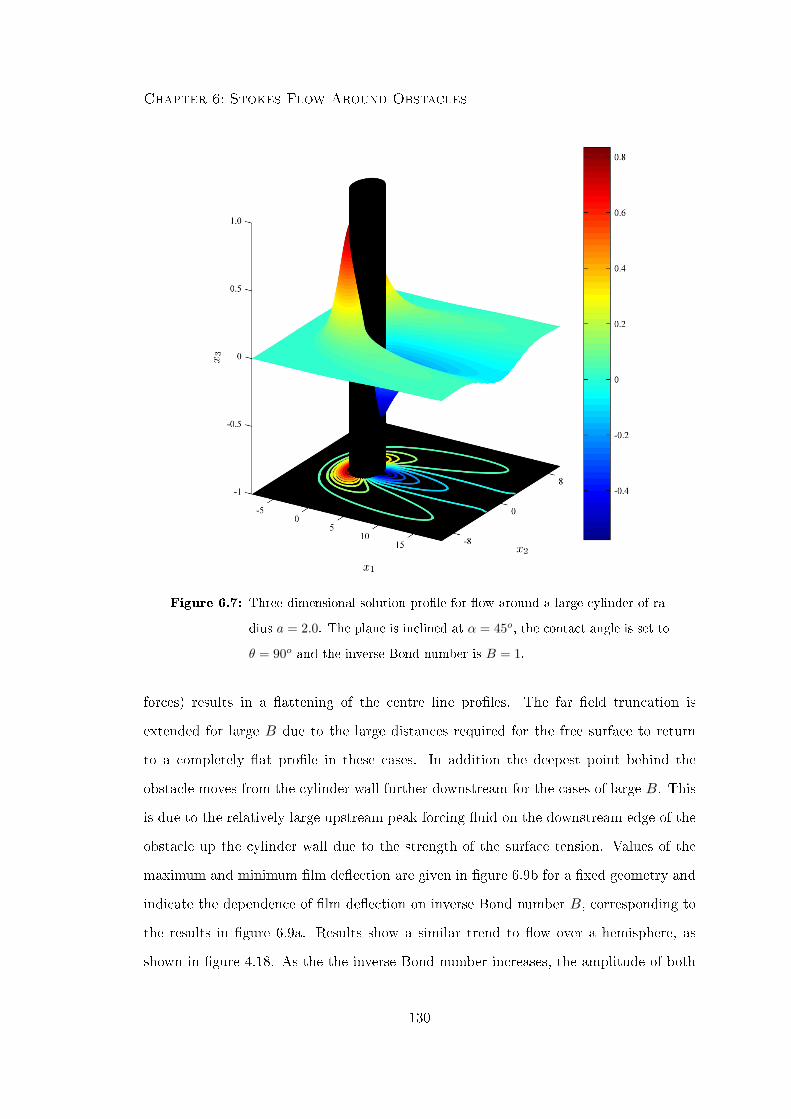
Chapter 6: Stokes Flow Around Obstacles
Figure 6.7: Three-dimensional solution prole for ow around a large cylinder of ra-
dius a = 2.0. The plane is inclined at α = 45o, the contact angle is set to
θ = 90o and the inverse Bond number is B = 1.
forces) results in a attening of the centre line proles. The far eld truncation is
extended for large B due to the large distances required for the free surface to return
to a completely at prole in these cases. In addition the deepest point behind the
obstacle moves from the cylinder wall further downstream for the cases of large B. This
is due to the relatively large upstream peak forcing uid on the downstream edge of the
obstacle up the cylinder wall due to the strength of the surface tension. Values of the
maximum and minimum lm deection are given in gure 6.9b for a xed geometry and
indicate the dependence of lm deection on inverse Bond number B, corresponding to
the results in gure 6.9a. Results show a similar trend to ow over a hemisphere, as
shown in gure 4.18. As the the inverse Bond number increases, the amplitude of both
130

Chapter 6: Stokes Flow Around Obstacles
Figure 6.8: Pattern of streamlines starting at x3 = −0.5 upstream of the cylinder and
for a range of x2 locations. Flow is around a circular cylinder of radius
a = 0.5, on a plane inclined at α = 45o. The ow has an inverse Bond
number of B = 1 and the contact angle is θ = 90o.
the peak and trough deection decrease. The peak heights are aected more severely due
to the higher curvature values in this region of the free surface. In addition, values for
peak height and trough depth appear to tend towards constant values as B is increased.
Figure 6.10 shows the contact line prole around the cylinder wall for the range of inverse
Bond numbers B depicted in gure 6.9. Raising the inverse Bond number attens the
ow proles around the cylinder wall. Intersection of the contact line proles occurs
over a relatively small range of angular positions along the cylinder, between 0.67− 1.06
radians upstream of the position x1 = a.
131

Chapter 6: Stokes Flow Around Obstacles
−10 −5 0 5 10 15−1
−0.5
0
0.5(a)
x1(x2 = 0)
x3
B = 1B = 5B = 10B = 15B = 20
0 2 4 6 8 10 12 14 16 18 20−0.2
−0.1
0
0.1
0.2
0.3
0.4
0.5(b)
B
x3
MaximumMinimum
Figure 6.9: Solutions for ow at various inverse Bond number B, down an inclined
plane at α = 45o around a cylinder of radius a = 0.5 and contact angle
θ = 90o. Part (a) shows centre line free surface elevations and (b) values
of maximum and minimum deection as inverse Bond number changes.
132

Chapter 6: Stokes Flow Around Obstacles
0 1 2 3 4 5 6
−0.1
−0.05
0
0.05
0.1
0.15
0.2
0.25
0.3
0.35
0.4
Angular Position On Cylinder
x3
B = 1B = 5B = 10B = 15B = 20
Figure 6.10: Contact line solutions for free surface deections on a plane inclined at
α = 45o around a cylinder of radius a = 0.5. The ow has various values
for inverse Bond number B. The contact angle at the cylinder wall is
θ = 90o.
Figure 6.11a illustrates solutions for a range of plane inclination angles α. Flow is for an
inverse Bond number B = 1 and around a cylindrical obstacle of radius a = 0.5. The free
surface/obstacle interface was modelled by a contact angle of θ = 90o. Increasing the
inclination angle results in a raising of the peak before the obstacle. The trough depth
behind the obstacle varies depending on the wall angle used. This is in comparison with
the earlier results for ow over hemispheres where a steeper plane inclination resulted
in a shallower trough behind the obstacle. The peak location in front of the obstacle
is unaected by a decrease in plane angle. Figure 6.11b illustrates the dependence of
maximum and minimum lm height on plane inclination angle, α, as seen in gure
6.11a. The values of peak lm height follow a similar trend to the results for ow over
a hemisphere as shown in gure 4.19. As the plane angle is increased the maximum lm
height increases, but at a progressively slower rate. The minimum lm height does not
133

Chapter 6: Stokes Flow Around Obstacles
follow the monotonic trend of gure 4.19; the trough is seen to initially deepen as the
plane inclination is raised, before becoming progressively less shallow.
Figure 6.12 illustrates the contact line prole around the cylinder wall for the range of
inclination angles depicted in gure 6.11. The steep planes cause a raise in the contact
height upstream of the obstacle.
Figure 6.13a shows the smoothed centre line solutions for ow around a range of cylinders
with varying radii. Flow is for an inverse Bond number B = 1 and down a plane inclined
at α = 45o. The obstacle was chosen to be neutrally wetting, (i.e. the contact angle
was θ = 90o). Increasing the cylinder radius results in a raising of the peak before the
obstacle and a deepening of the trough behind it. This is a similar trend to that found
earlier, and shown in gure 4.9. Figure 6.13b shows values of maximum and minimum
lm deection for solutions shown in gure 6.13a, indicating the dependence of lm
deection on cylinder radius, a. There is an approximately linear dependence for both
cases, with the maximum lm height increasing and the minimum lm height decreasing,
with cylinder radius.
Figure 6.14 illustrates the contact line prole around the cylinder wall for the range of
cylinder radii depicted in gure 6.13. The large cylinders cause a rise in the contact height
upstream of the obstacle and a lowering of the contact height downstream. Interestingly,
intersection of the contact line proles occurs at an approximately xed angular position
along the cylinder, between 0.94−0.98 radians upstream of the position x1 = a. Further
renement of the mesh around the cylinder may cause this range of angular position to
diminish.
Figure 6.15a shows the smoothed centre line solutions for ow around a cylinder of
radius 0.5. Flow is for an inverse Bond number B = 1 and down a plane inclined at
α = 45o. The solutions show a range of wetting and non-wetting ow congurations
corresponding to a range of contact angles θ. Decreasing the contact angle results in
a raising of both the peak height before the obstacle and the trough behind it. In
134

Chapter 6: Stokes Flow Around Obstacles
−8 −6 −4 −2 0 2 4 6 8 10−1
−0.8
−0.6
−0.4
−0.2
0
0.2
0.4
0.6(a)
x1(x2 = 0)
x3
α = 90o
α = 45o
α = 27o
α = 9o
0 10 20 30 40 50 60 70 80 90 100−0.2
−0.1
0
0.1
0.2
0.3
0.4
0.5
0.6
0.7(b)
α
x3
MaximumMinimum
Figure 6.11: Solutions for ow around a cylinder of radius a = 0.5 and contact angle
θ = 90o with an inverse Bond number B = 1 and down a plane of various
inclinations. Part (a) indicates the centre line solutions and (b) values
of maximum and minimum deection as the plane inclination changes.
135

Chapter 6: Stokes Flow Around Obstacles
0 1 2 3 4 5 6
−0.1
0
0.1
0.2
0.3
0.4
0.5
Angular Position On Cylinder
x3
α = 90o
α = 45o
α = 27o
α = 9o
Figure 6.12: Contact line solutions for free surface deections for ow down a plane
at various inclination angles and around a cylinder of radius a = 0.5.
The ow has an inverse Bond number of B = 1 and the contact angle
at the cylinder wall is θ = 90o.
addition for wetting obstacles, maximum peak height occurs on the cylinder wall instead
of a small distance from the cylinder. In contrast the non-wetting obstacles cause the
minimum of the trough to occur at the cylinder instead of a small distance downstream
of the obstacle. Figure 6.15b shows the trend of maximum and minimum lm height for
contact angle θ, with values corresponding to the results in gure 6.15a. Results show
that for θ ≤ 90o, the maximum heights decrease approximately linearly with increasing
θ, and corresponds to lm proles where the peak occurs at the cylinder wall. Maximum
heights for θ > 90o decrease at a slower rate, corresponding to peak lm heights occurring
away from the cylinder wall. For θ < 90o but increasing, the trough depth decreases at a
slow rate, corresponding to cases where the lm minimum occurs away from the cylinder
wall. For θ ≥ 90o, minimum heights decrease more quickly, and approximately linearly
with increasing θ, corresponding to results where the lm minimum occurs against the
136
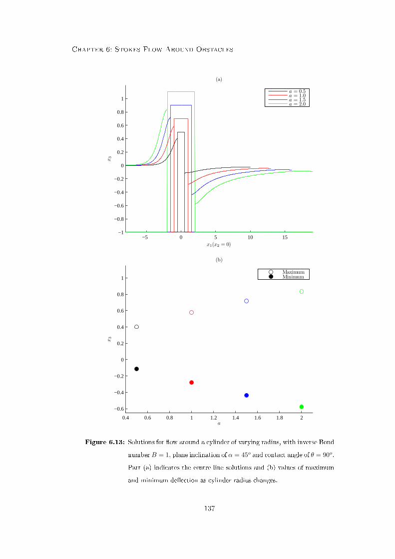
Chapter 6: Stokes Flow Around Obstacles
−5 0 5 10 15−1
−0.8
−0.6
−0.4
−0.2
0
0.2
0.4
0.6
0.8
1
(a)
x1(x2 = 0)
x3
a = 0.5a = 1.0a = 1.5a = 2.0
0.4 0.6 0.8 1 1.2 1.4 1.6 1.8 2
−0.6
−0.4
−0.2
0
0.2
0.4
0.6
0.8
1
(b)
a
x3
MaximumMinimum
Figure 6.13: Solutions for ow around a cylinder of varying radius, with inverse Bond
number B = 1, plane inclination of α = 45o and contact angle of θ = 90o.
Part (a) indicates the centre line solutions and (b) values of maximum
and minimum deection as cylinder radius changes.
137

Chapter 6: Stokes Flow Around Obstacles
0 1 2 3 4 5 6−0.6
−0.4
−0.2
0
0.2
0.4
0.6
0.8
1
Angular Position On Cylinder
x3
a = 0.5a = 1.0a = 1.5a = 2.0
Figure 6.14: Contact line solutions for free surface deections around a cylinder of
varying radius, with inverse Bond number B = 1 and down a plane
inclined at α = 45o. The contact angle at the cylinder wall is θ = 90o.
cylinder wall.
Figure 6.16 shows the contact line proles around the cylinder wall for the range of con-
tact angles depicted in gure 6.15. As the contact angle is raised, the contact line prole
becomes sharper due to its greater eect downstream than upstream of the cylinder.
6.3.2 Multiple Solutions
The existence of multiple solutions for ow down a vertical plane will be demonstrated.
Multiple solutions occur, when for the same ow parameters (i.e. Bond number, plane
angle and obstacle geometry), ow can either exist completely submerging the obstacle
or owing around the obstacle. Take α = 90o, Bo = 1 and a cylinder radius a = 0.5,
and for ow around a cylinder the static contact line angle is set at θ = 105o. The
138

Chapter 6: Stokes Flow Around Obstacles
−8 −6 −4 −2 0 2 4 6 8 10−1
−0.8
−0.6
−0.4
−0.2
0
0.2
0.4
0.6
0.8(a)
x1(x2 = 0)
x3
θ = 50o
θ = 70o
θ = 90o
θ = 110o
θ = 130o
50 60 70 80 90 100 110 120 130−0.6
−0.4
−0.2
0
0.2
0.4
0.6
0.8(b)
θ
x3
MaximumMinimum
Figure 6.15: Solutions for various contact angles applied at the cylinder of radius
a = 0.5 attached to a plane inclined at α = 45o. The ow has an inverse
Bond number B = 1. Part (a) indicates the centre line solutions and (b)
values of maximum and minimum deection for various contact angles.
139

Chapter 6: Stokes Flow Around Obstacles
0 1 2 3 4 5 6−0.6
−0.4
−0.2
0
0.2
0.4
0.6
0.8
Angular Position On Cylinder
x3
θ = 50o
θ = 70o
θ = 90o
θ = 110o
θ = 130o
Figure 6.16: Contact line solutions for various contact angles at the cylinder wall.
The free surface deections are around a cylinder of radius a = 0.5 on
an inclined plane at α = 45o and the ow has an inverse Bond number
B = 1.
free surface was solved in the domain −8 ≤ x1 ≤ 10 and −8 ≤ x2 ≤ 8 with the zero
gradient far eld conditions implemented. For the outer mesh, and for the complete ow-
over mesh the surface was discretized into 36× 32 elements (neglecting an inner rened
region for the ow-over discretization). The previous transitional mesh for ow around
the cylinder was retained, utilizing 6 elements with scaling factor 0.65. The cylinder
was discretized by splitting the walls into ve rows of elements, and the circumferential
mesh (and top) of the cylinder was generated by four successive subdivisions. For ow
over the cylinder, a parameter continuation method is adopted as for the case of large
hemispherical obstacles already considered. This allows the cylinder to be increased
above the undisturbed lm height, allowing multiple solutions to be found.
Figure 6.17 indicates that the ow prole around a cylinder is below the top of the
truncated cylinder used to obtain ows over a cylinder. The truncated cylinder varies
140

Chapter 6: Stokes Flow Around Obstacles
0 1 2 3 4 5 6−0.3
−0.2
−0.1
0
0.1
0.2
0.3
0.4
0.5
Angular Position On Cylinder
x3
Cylinder TopContact Line
Figure 6.17: Comparison of the sloped cylinder top between x3 = 0.42 and x3 = 0.12,
and contact line for ow around the cylinder of radius a = 0.5. The ow
is down a vertical plane (α = 90o), with a Bond number Bo = 1.0, and
a contact angle of θ = 105o.
linearly between x3 = 0.42 and x3 = 0.12. Thus multiple solutions exist for this set of
ow parameters. Figure 6.18 indicates the corresponding centre line solutions for x2 = 0
and x1 = 0. The ow intersected by the obstacle is subject to a 105o contact angle,
and as such it is clearly seen that any more severely non-wetting obstacle can exhibit
multiple solutions in this scenario.
For ow over or around a given cylinder, the existence of multiple solutions for varying
ow parameters can be examined. Analysis is conducted for a cylinder of radius a = 0.5
with top sloped linearly in the x1 direction between heights x3 = 0.3 and x3 = 0.0. The
cylinder geometry is xed and possible multiple solutions obtained for variations in the
inverse Bond number B, and plane inclination angle α. For ow around the cylinder,
three contact angles are analyzed, θ = 90o, 105o, 120o. Possible multiple solutions are
141
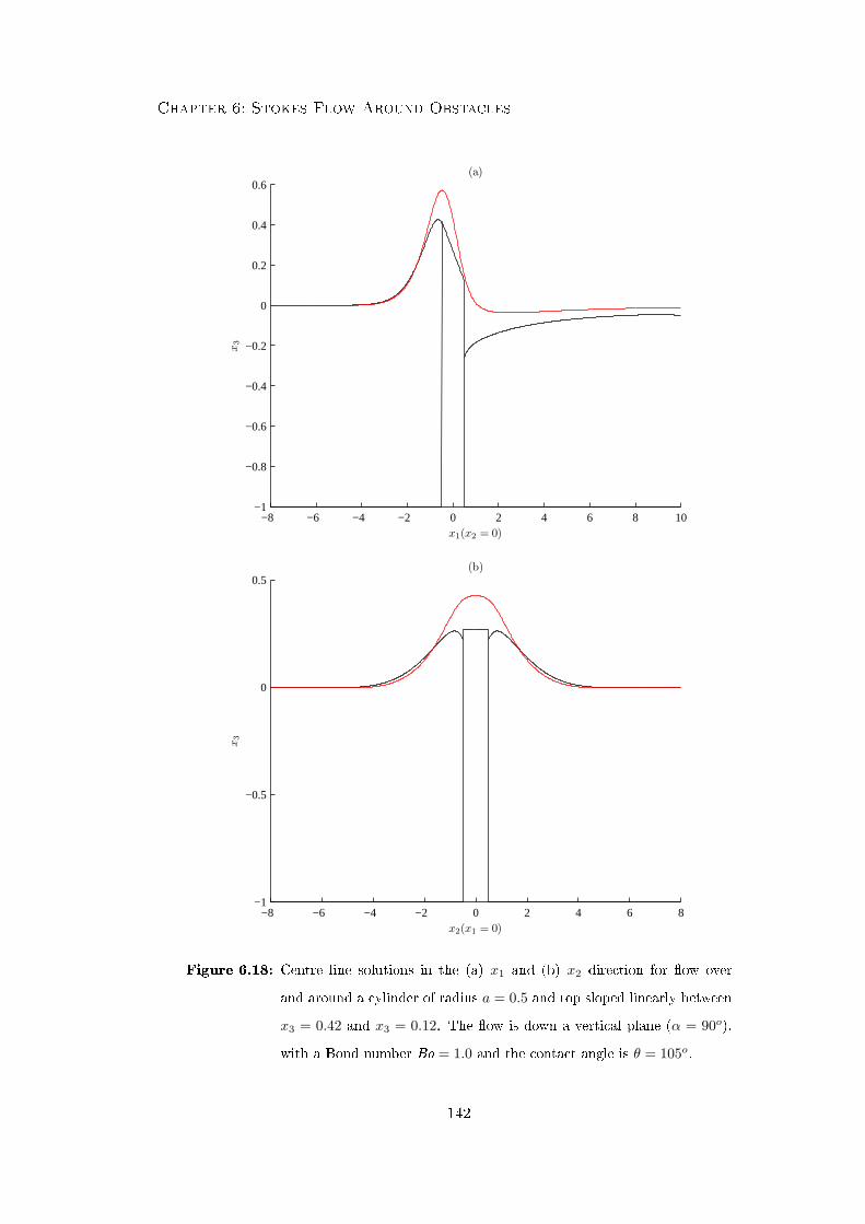
Chapter 6: Stokes Flow Around Obstacles
−8 −6 −4 −2 0 2 4 6 8 10−1
−0.8
−0.6
−0.4
−0.2
0
0.2
0.4
0.6(a)
x1(x2 = 0)
x3
−8 −6 −4 −2 0 2 4 6 8−1
−0.5
0
0.5(b)
x2(x1 = 0)
x3
Figure 6.18: Centre line solutions in the (a) x1 and (b) x2 direction for ow over
and around a cylinder of radius a = 0.5 and top sloped linearly between
x3 = 0.42 and x3 = 0.12. The ow is down a vertical plane (α = 90o),
with a Bond number Bo = 1.0 and the contact angle is θ = 105o.
142
Chapter 6: Stokes Flow Around Obstacles
characterized by the maximum lm height of the uid ow.
Figure 6.19 provides a map of solutions, characterized by maximum lm height, for ow
over or around the prescribed cylinder for variations in the inverse Bond number B.
The plane inclination is xed at α = 90o. Black lines indicate results for ow over the
cylinder, and coloured lines results for ow around the cylinder for the three selected
contact angles. Results are produced for the values of B indicated in the gure. For
ow over the cylinder, an inverse Bond number of B = 1 is considered, and progressively
increased. Numerical simulations are successful up to and including B = 1.6, with the
numerical method found to fail within the region 1.6 < B ≤ 2. This is indicated in
the gure by | → and is a consequence of the free surface impinging on the top of the
truncated cylinder. For ow around the cylinder, results are obtained for B = 5, and the
inverse Bond number is progressively reduced until the ow no longer remains below the
top edge of the cylinder with failure indicated in the gure by ← |. For θ = 90o results
are obtained for B ≥ 3.5, with failure in the region 3 ≤ B < 3.5 and for θ = 105o results
are found for B ≥ 1.6, with failure in the region 1.2 ≤ B < 1.6. When a contact angle
of θ = 120o is used, results are obtained for all B considered. For values of B ≤ 1.6, two
distinct solution are possible corresponding to both ow over and ow around a circular
cylinder of nite height. In all cases the regions of failure can be rened by evaluation
of the ow at a greater number of inverse Bond numbers.
Figure 6.20 indicates the existence of possible twin solutions, characterized by maximum
lm height, for ow over or around the prescribed cylinder for variations in the plane
inclination angle α. The inverse Bond number of the ow is constrained to B = 1. A
black line indicates results obtained for ow over the cylinder, and coloured lines results
for ow around the cylinder with the three dierent contact angles prescribed. Results
are produced for the values of α indicated in the gure. When ow is over the cylinder,
a plane inclination of α = 90o is considered, and progressively reduced. Numerical
simulations are successful for plane angles down to and including α = 54o, with failure
of the numerical method in the region 45o ≤ α < 54o. This is indicated in the gure
143
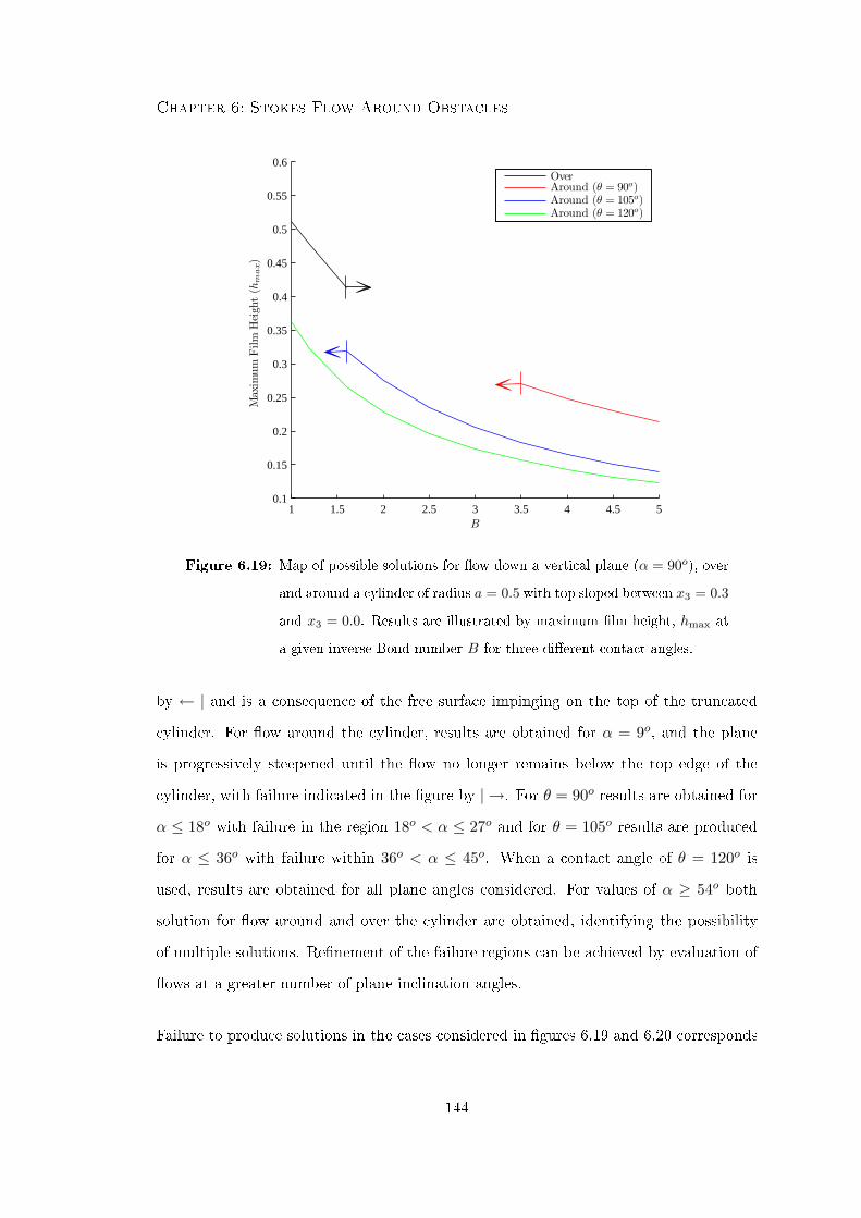
Chapter 6: Stokes Flow Around Obstacles
1 1.5 2 2.5 3 3.5 4 4.5 50.1
0.15
0.2
0.25
0.3
0.35
0.4
0.45
0.5
0.55
0.6
B
Max
imum
Film
Heigh
t(h
ma
x)
OverAround (θ = 90o)Around (θ = 105o)Around (θ = 120o)
Figure 6.19: Map of possible solutions for ow down a vertical plane (α = 90o), over
and around a cylinder of radius a = 0.5 with top sloped between x3 = 0.3
and x3 = 0.0. Results are illustrated by maximum lm height, hmax at
a given inverse Bond number B for three dierent contact angles.
by ← | and is a consequence of the free surface impinging on the top of the truncated
cylinder. For ow around the cylinder, results are obtained for α = 9o, and the plane
is progressively steepened until the ow no longer remains below the top edge of the
cylinder, with failure indicated in the gure by | →. For θ = 90o results are obtained for
α ≤ 18o with failure in the region 18o < α ≤ 27o and for θ = 105o results are produced
for α ≤ 36o with failure within 36o < α ≤ 45o. When a contact angle of θ = 120o is
used, results are obtained for all plane angles considered. For values of α ≥ 54o both
solution for ow around and over the cylinder are obtained, identifying the possibility
of multiple solutions. Renement of the failure regions can be achieved by evaluation of
ows at a greater number of plane inclination angles.
Failure to produce solutions in the cases considered in gures 6.19 and 6.20 corresponds
144
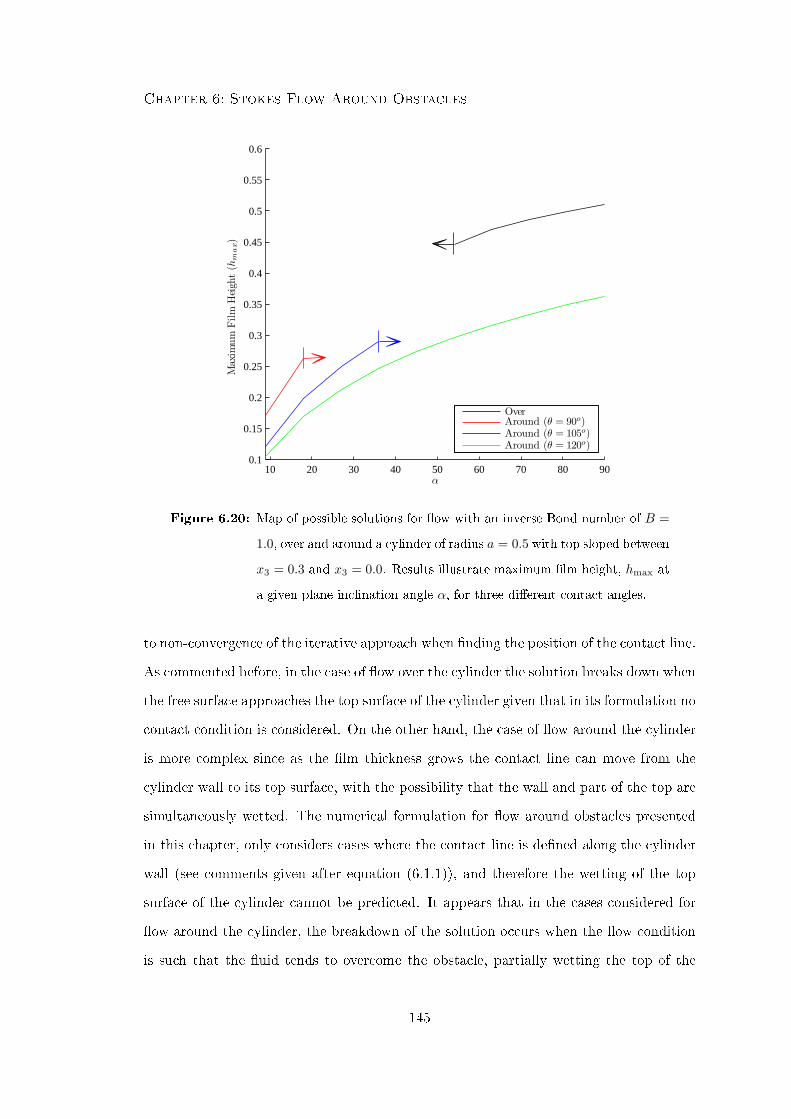
Chapter 6: Stokes Flow Around Obstacles
10 20 30 40 50 60 70 80 900.1
0.15
0.2
0.25
0.3
0.35
0.4
0.45
0.5
0.55
0.6
α
Max
imum
Film
Heigh
t(h
ma
x)
OverAround (θ = 90o)Around (θ = 105o)Around (θ = 120o)
Figure 6.20: Map of possible solutions for ow with an inverse Bond number of B =
1.0, over and around a cylinder of radius a = 0.5 with top sloped between
x3 = 0.3 and x3 = 0.0. Results illustrate maximum lm height, hmax at
a given plane inclination angle α, for three dierent contact angles.
to non-convergence of the iterative approach when nding the position of the contact line.
As commented before, in the case of ow over the cylinder the solution breaks down when
the free surface approaches the top surface of the cylinder given that in its formulation no
contact condition is considered. On the other hand, the case of ow around the cylinder
is more complex since as the lm thickness grows the contact line can move from the
cylinder wall to its top surface, with the possibility that the wall and part of the top are
simultaneously wetted. The numerical formulation for ow around obstacles presented
in this chapter, only considers cases where the contact line is dened along the cylinder
wall (see comments given after equation (6.1.1)), and therefore the wetting of the top
surface of the cylinder cannot be predicted. It appears that in the cases considered for
ow around the cylinder, the breakdown of the solution occurs when the ow condition
is such that the uid tends to overcome the obstacle, partially wetting the top of the
145
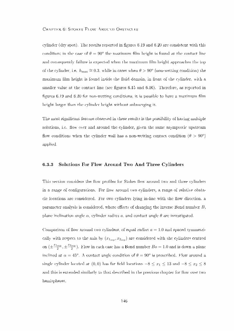
Chapter 6: Stokes Flow Around Obstacles
cylinder (dry spot). The results reported in gures 6.19 and 6.20 are consistent with this
condition; in the case of θ = 90o the maximum lm height is found at the contact line
and consequently failure is expected when the maximum lm height approaches the top
of the cylinder, i.e. hmax∼= 0.3, while in cases when θ > 90o (non-wetting condition) the
maximum lm height is found inside the uid domain, in front of the cylinder, with a
smaller value at the contact line (see gures 6.15 and 6.16). Therefore, as reported in
gures 6.19 and 6.20 for non-wetting conditions, it is possible to have a maximum lm
height larger than the cylinder height without submerging it.
The most signicant feature observed in these results is the possibility of having multiple
solutions, i.e. ow over and around the cylinder, given the same asymptotic upstream
ow conditions when the cylinder wall has a non-wetting contact condition (θ > 90o)
applied.
6.3.3 Solutions For Flow Around Two And Three Cylinders
This section considers the ow proles for Stokes ow around two and three cylinders
in a range of congurations. For ow around two cylinders, a range of relative obsta-
cle locations are considered. For two cylinders lying in-line with the ow direction, a
parameter analysis is considered, where eects of changing the inverse Bond number B,
plane inclination angle α, cylinder radius a, and contact angle θ are investigated.
Comparison of ow around two cylinders, of equal radius a = 1.0 and spaced symmetri-
cally with respect to the axis by (x1sep , x2sep) are considered with the cylinders centred
on (±x1sep
2 ,±x2sep
2 ). Flow in each case has a Bond number Bo = 1.0 and is down a plane
inclined at α = 45o. A contact angle condition of θ = 90o is prescribed. Flow around a
single cylinder located at (0, 0) has far eld locations −8 ≤ x1 ≤ 13 and −8 ≤ x2 ≤ 8
and this is extended similarly to that described in the previous chapter for ow over two
hemispheres.
146

Chapter 6: Stokes Flow Around Obstacles
Figure 6.21 illustrates the centre line (x2 = 0) proles of surface elevation for ow
around two cylinders in-line with the incident ow and with various spacings. Compar-
ison proles are given for ow around a single cylinder at (±x1sep
2 , 0). For all cases of
obstacle separation, the ow prole generated by the upstream cylinder appears to be
close to the prole for a single cylinder. When the separation is increased, ow around
the downstream cylinder approximates more closely the deformation caused by a single
obstacle. As the separation increases the wake decays after the leading cylinder and
the incident ow conguration to the rear obstacle approaches that of an undisturbed
ow. As the obstacles are moved closer together the peak height incident on the cylinder
wall decreases. For x1sep ≥ 6, the ow around the rear obstacle stems from the same
location on the back edge of the upstream cylinder. The ow height on the back edge of
the downstream cylinder is slightly reduced as the obstacles are brought closer together,
although any changes are small. For x1sep = 4, the prole fundamentally changes, with
the lm height on the back edge of the upstream cylinder raised signicantly, and the
lm height at the upstream edge of the rear cylinder lowered. The ow prole in this
case is shown as a contour plot in gure 6.24, for x1sep = 4 and x2sep = 0.
Figure 6.22 shows the centre line (x1 = 0) proles for ow around two cylinders symmet-
rically positioned perpendicular to the incoming ow direction. Dashed proles indicate
the ow proles around a single cylinder at (0,±x2sep
2 ). For large separations (x2sep ≥ 6),
the proles around the double obstacle are accurately approximated by the ow proles
for two single obstacles, with the outer regions of the ow proles remaining consistent
with the corresponding single obstacle solution. The lowest free surface height in the
merged inner region of the ow slowly increases from the undisturbed lm height as the
cylinders are brought closer together. For x2sep = 4, the outer regions of the ow prole
dier from the corresponding single obstacle analysis, with a raised contact point on the
cylinder wall. The lm height of the inner region is raised signicantly as the ow is
forced through the small gap between the cylinders. A contour plot of this prole is
shown in gure 6.24, for x1sep = 0 and x2sep = 4.
147

Chapter 6: Stokes Flow Around Obstacles
−10 −5 0 5 10 15−1
−0.5
0
0.5
1
x1(x1sep = 4) (x2 = 0)
x3
−10 −5 0 5 10 15−1
−0.5
0
0.5
1
x1(x1sep = 6) (x2 = 0)
x3
−10 −5 0 5 10 15−1
−0.5
0
0.5
1
x1(x1sep = 8) (x2 = 0)
x3
−10 −5 0 5 10 15−1
−0.5
0
0.5
1
x1(x1sep = 10) (x2 = 0)
x3
Figure 6.21: Centre line proles for various cylinder separations x1sepin line with the
ow. The ow has a Bond number of Bo = 1.0, is down a plane inclined
at α = 45o, and the cylinder has a radius of a = 1.0, and contact angle
of θ = 90o.
148
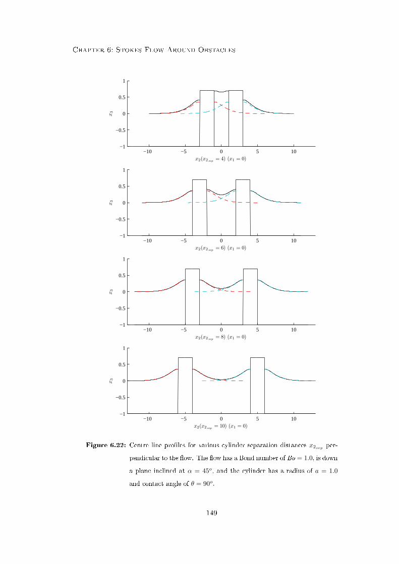
Chapter 6: Stokes Flow Around Obstacles
−10 −5 0 5 10−1
−0.5
0
0.5
1
x2(x2sep = 4) (x1 = 0)
x3
−10 −5 0 5 10−1
−0.5
0
0.5
1
x2(x2sep = 6) (x1 = 0)
x3
−10 −5 0 5 10−1
−0.5
0
0.5
1
x2(x2sep = 8) (x1 = 0)
x3
−10 −5 0 5 10−1
−0.5
0
0.5
1
x2(x2sep = 10) (x1 = 0)
x3
Figure 6.22: Centre line proles for various cylinder separation distances x2sep per-
pendicular to the ow. The ow has a Bond number of Bo = 1.0, is down
a plane inclined at α = 45o, and the cylinder has a radius of a = 1.0
and contact angle of θ = 90o.
149

Chapter 6: Stokes Flow Around Obstacles
Figure 6.23: Three-dimensional solution prole for two cylinders separated by x1sep =
4, x2sep= 4. Flow parameters are; Bo = 1.0, a = 1.0, α = 45o, and
θ = 90o.
Figure 6.23 shows the full free surface for the analysis of ow around two o-set cylinders
separated by x1sep = x2sep = 4. The ow is incident to the rst cylinder, and as the
ow peak splits around the obstacle, one of these raised ridges is incident onto the
downstream cylinder. This thicker lm region causes the peak formed around the rear
cylinder to increase, before decaying with a typical wake structure for a single cylinder.
The individual proles around each cylinder are suciently close to exhibit interaction
with each other as is illustrated by the associated contour plot in gure 6.24.
Figure 6.24 illustrates three contour plots for the obstacle congurations corresponding
to gures 6.21, 6.22 and 6.23. Taking x1sep = 4, x2sep = 0 the ow is symmetric about
150

Chapter 6: Stokes Flow Around Obstacles
x2 = 0 and the highest points on the free surface occur on the upstream edge of the
two cylinders. The rapid rise in lm height is shown between the two cylinders as the
trough from the leading cylinder develops into the peak of the downstream obstacle.
The centre line plot for this ow can also be seen in gure 6.21. The contour plot for
the case x1sep = 0, x2sep = 4 illustrates just a single, wide peak occurring and covering
the leading edges of the two cylinders. The peak decays into a trough just behind
each of the cylinders, with the raised ow forced between the cylinders decaying to the
undisturbed lm height further downstream. The contour plot for the non-symmetric
case x1sep = 4, x2sep = 4 shows the contours of ow around two o-set cylinders with the
downstream cylinder generating a slightly larger peak. The rear cylinder is seen to lie
in the decaying peak of the upstream cylinder causing the range of this peak to extend
further downstream.
A parameter analysis is conducted demonstrating the eects of altering the inverse Bond
number B, plane inclination angle α, obstacle radii a, and contact angle θ. An inline
conguration with x1sep = 8 is taken. Default values for the ow parameters include an
inverse Bond number of B = 1, a plane inclination angle of α = 45o, circular cylinders of
radius a = 1.0, and a contact angle condition of θ = 90o. In each case, three parameters
are chosen from above and the eects of altering the fourth analyzed.
Figure 6.25 illustrates the surface elevation along the centre line (x2 = 0) for variations
in inverse Bond number, with an increase in B showing a attening and smoothing of
the proles associated with an increase in surface tension. For B = 1, the centre line
proles undergo large variations in lm height. The eects of increasing B is to raise the
lowest points and lower the highest points of the lm, minimizing the deformation of the
free surface. In common with the single obstacle analysis shown in gure 6.9 and the
earlier dual hemisphere analysis, the inverse Bond number causes the lm disturbance
to span a greater region upstream in the x1 direction.
Figure 6.26 illustrates the centre line (x2 = 0) surface elevations for changes in the plane
151

Chapter 6: Stokes Flow Around Obstacles
Figure 6.24: Contour plots for (x1sep, x2sep
) = (4, 0), (0, 4), (4, 4), for ow around
cylinders of radius a = 1.0. Other ow parameters are; Bo = 1.0,
α = 45o, and θ = 90o.
152
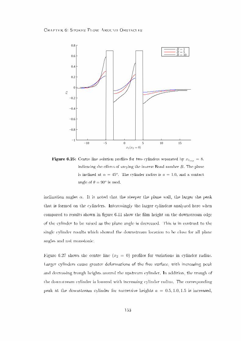
Chapter 6: Stokes Flow Around Obstacles
−10 −5 0 5 10 15−1
−0.8
−0.6
−0.4
−0.2
0
0.2
0.4
0.6
0.8
x1(x2 = 0)
x3
B = 1B = 5B = 10
Figure 6.25: Centre line solution proles for two cylinders separated by x1sep = 8,
indicating the eects of varying the inverse Bond number B. The plane
is inclined at α = 45o. The cylinder radius is a = 1.0, and a contact
angle of θ = 90o is used.
inclination angles α. It is noted that the steeper the plane wall, the larger the peak
that is formed on the cylinders. Interestingly the larger cylinders analyzed here when
compared to results shown in gure 6.11 show the lm height on the downstream edge
of the cylinder to be raised as the plane angle is decreased. This is in contrast to the
single cylinder results which showed the downstream location to be close for all plane
angles and not monotonic.
Figure 6.27 shows the centre line (x2 = 0) proles for variations in cylinder radius.
Larger cylinders cause greater deformations of the free surface, with increasing peak
and decreasing trough heights around the upstream cylinder. In addition, the trough of
the downstream cylinder is lowered with increasing cylinder radius. The corresponding
peak at the downstream cylinder for successive heights a = 0.5, 1.0, 1.5 is increased,
153
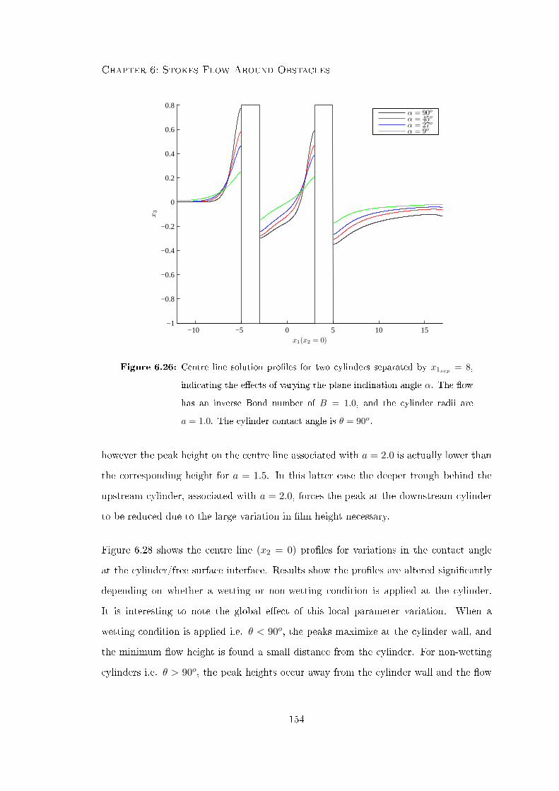
Chapter 6: Stokes Flow Around Obstacles
−10 −5 0 5 10 15−1
−0.8
−0.6
−0.4
−0.2
0
0.2
0.4
0.6
0.8
x1(x2 = 0)
x3
α = 90o
α = 45o
α = 27o
α = 9o
Figure 6.26: Centre line solution proles for two cylinders separated by x1sep= 8,
indicating the eects of varying the plane inclination angle α. The ow
has an inverse Bond number of B = 1.0, and the cylinder radii are
a = 1.0. The cylinder contact angle is θ = 90o.
however the peak height on the centre line associated with a = 2.0 is actually lower than
the corresponding height for a = 1.5. In this latter case the deeper trough behind the
upstream cylinder, associated with a = 2.0, forces the peak at the downstream cylinder
to be reduced due to the large variation in lm height necessary.
Figure 6.28 shows the centre line (x2 = 0) proles for variations in the contact angle
at the cylinder/free surface interface. Results show the proles are altered signicantly
depending on whether a wetting or non-wetting condition is applied at the cylinder.
It is interesting to note the global eect of this local parameter variation. When a
wetting condition is applied i.e. θ < 90o, the peaks maximize at the cylinder wall, and
the minimum ow height is found a small distance from the cylinder. For non-wetting
cylinders i.e. θ > 90o, the peak heights occur away from the cylinder wall and the ow
154

Chapter 6: Stokes Flow Around Obstacles
−10 −5 0 5 10 15 20−1
−0.8
−0.6
−0.4
−0.2
0
0.2
0.4
0.6
0.8
1
x1(x2 = 0)
x3
a = 0.5a = 1.0a = 1.5a = 2.0
Figure 6.27: Centre line solution proles for two cylinders separated by x1sep= 8,
indicating the eects of varying the cylinders radii a. The ows inverse
Bond number is B = 1.0, and the plane is inclined at α = 45o. The
contact angle at the contact line is θ = 90o.
height minimizes at the point of contact. These results are consistent with the case of a
single cylinder (see gure 6.15).
The ow around three cylinders in two geometrical congurations is considered. Flow
is taken down a plane inclined at α = 45o and has a Bond number Bo = 1. Flow is
around circular cylinders of radius a = 1.0, with a contact angle condition of θ = 90o
applied. Cylinders are positioned in a symmetrical triangular array, with either a twin
or single leading cylinder considered. A twin leading conguration is illustrated in gure
6.29 and consists of the upstream ow incident on two cylinders spaced perpendicularly
to the ow direction at centres (−2,−2), (−2, 2). This is followed by a trailing cylinder
centered at (2, 0). The conguration shown in gure 6.30 consists of the upstream ow
incident on one obstacle centered at (−2, 0) followed by two downstream cylinders spaced
155
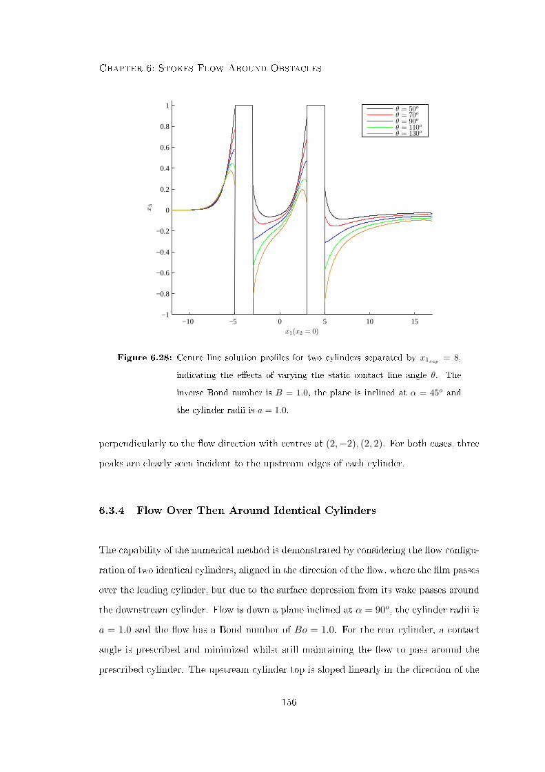
Chapter 6: Stokes Flow Around Obstacles
−10 −5 0 5 10 15−1
−0.8
−0.6
−0.4
−0.2
0
0.2
0.4
0.6
0.8
1
x1(x2 = 0)
x3
θ = 50o
θ = 70o
θ = 90o
θ = 110o
θ = 130o
Figure 6.28: Centre line solution proles for two cylinders separated by x1sep= 8,
indicating the eects of varying the static contact line angle θ. The
inverse Bond number is B = 1.0, the plane is inclined at α = 45o and
the cylinder radii is a = 1.0.
perpendicularly to the ow direction with centres at (2,−2), (2, 2). For both cases, three
peaks are clearly seen incident to the upstream edges of each cylinder.
6.3.4 Flow Over Then Around Identical Cylinders
The capability of the numerical method is demonstrated by considering the ow congu-
ration of two identical cylinders, aligned in the direction of the ow, where the lm passes
over the leading cylinder, but due to the surface depression from its wake passes around
the downstream cylinder. Flow is down a plane inclined at α = 90o, the cylinder radii is
a = 1.0 and the ow has a Bond number of Bo = 1.0. For the rear cylinder, a contact
angle is prescribed and minimized whilst still maintaining the ow to pass around the
prescribed cylinder. The upstream cylinder top is sloped linearly in the direction of the
156
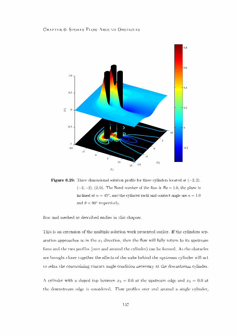
Chapter 6: Stokes Flow Around Obstacles
Figure 6.29: Three-dimensional solution prole for three cylinders located at (−2, 2),
(−2,−2), (2, 0). The Bond number of the ow is Bo = 1.0, the plane is
inclined at α = 45o, and the cylinder radii and contact angle are a = 1.0
and θ = 90o respectively.
ow and meshed as described earlier in this chapter.
This is an extension of the multiple solution work presented earlier. If the cylinders sep-
aration approaches ∞ in the x1 direction, then the ow will fully return to its upstream
form and the two proles (over and around the cylinder) can be formed. As the obstacles
are brought closer together the eects of the wake behind the upstream cylinder will act
to relax the constraining contact angle condition necessary at the downstream cylinder.
A cylinder with a sloped top between x3 = 0.6 at the upstream edge and x3 = 0.0 at
the downstream edge is considered. Flow proles over and around a single cylinder,
157
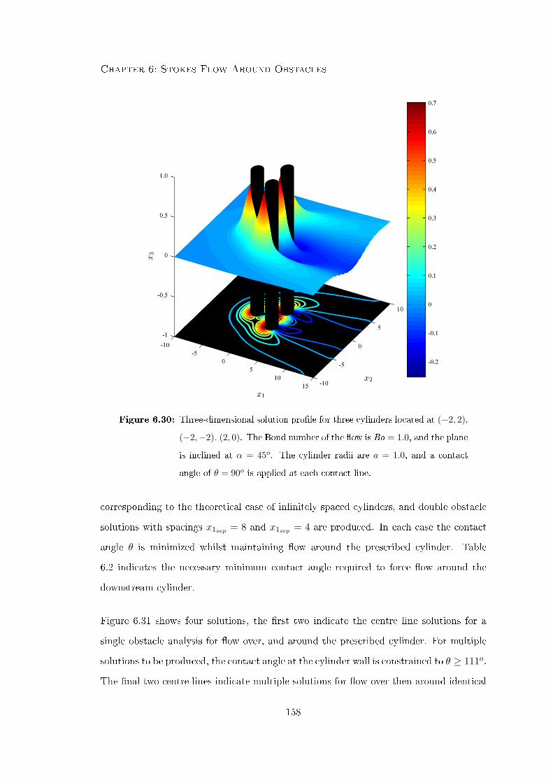
Chapter 6: Stokes Flow Around Obstacles
Figure 6.30: Three-dimensional solution prole for three cylinders located at (−2, 2),
(−2,−2), (2, 0). The Bond number of the ow is Bo = 1.0, and the plane
is inclined at α = 45o. The cylinder radii are a = 1.0, and a contact
angle of θ = 90o is applied at each contact line.
corresponding to the theoretical case of innitely spaced cylinders, and double obstacle
solutions with spacings x1sep = 8 and x1sep = 4 are produced. In each case the contact
angle θ is minimized whilst maintaining ow around the prescribed cylinder. Table
6.2 indicates the necessary minimum contact angle required to force ow around the
downstream cylinder.
Figure 6.31 shows four solutions, the rst two indicate the centre line solutions for a
single obstacle analysis for ow over, and around the prescribed cylinder. For multiple
solutions to be produced, the contact angle at the cylinder wall is constrained to θ ≥ 111o.
The nal two centre lines indicate multiple solutions for ow over then around identical
158
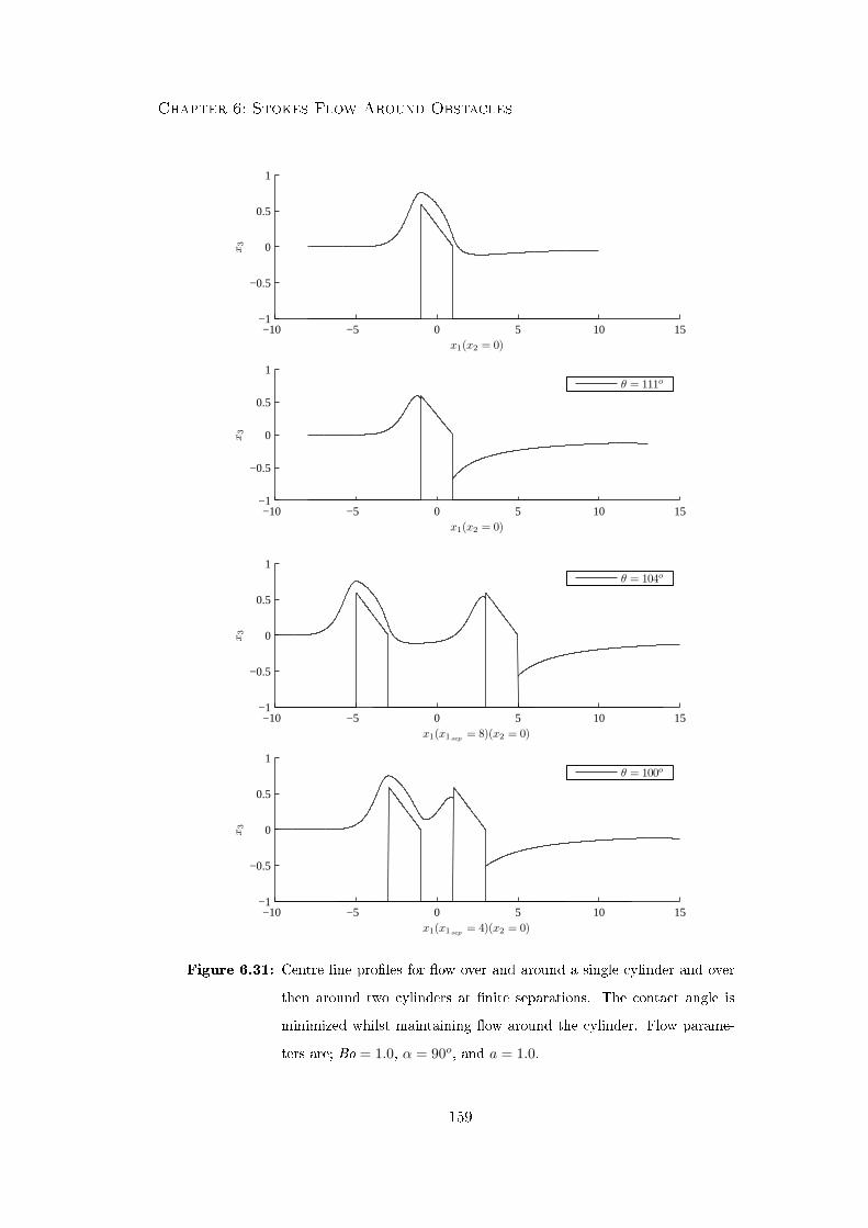
Chapter 6: Stokes Flow Around Obstacles
−10 −5 0 5 10 15−1
−0.5
0
0.5
1
x1(x2 = 0)
x3
−10 −5 0 5 10 15−1
−0.5
0
0.5
1
x1(x2 = 0)
x3
−10 −5 0 5 10 15−1
−0.5
0
0.5
1
x1(x1sep = 8)(x2 = 0)
x3
−10 −5 0 5 10 15−1
−0.5
0
0.5
1
x1(x1sep = 4)(x2 = 0)
x3
θ = 111o
θ = 104o
θ = 100o
Figure 6.31: Centre line proles for ow over and around a single cylinder and over
then around two cylinders at nite separations. The contact angle is
minimized whilst maintaining ow around the cylinder. Flow parame-
ters are; Bo = 1.0, α = 90o, and a = 1.0.
159
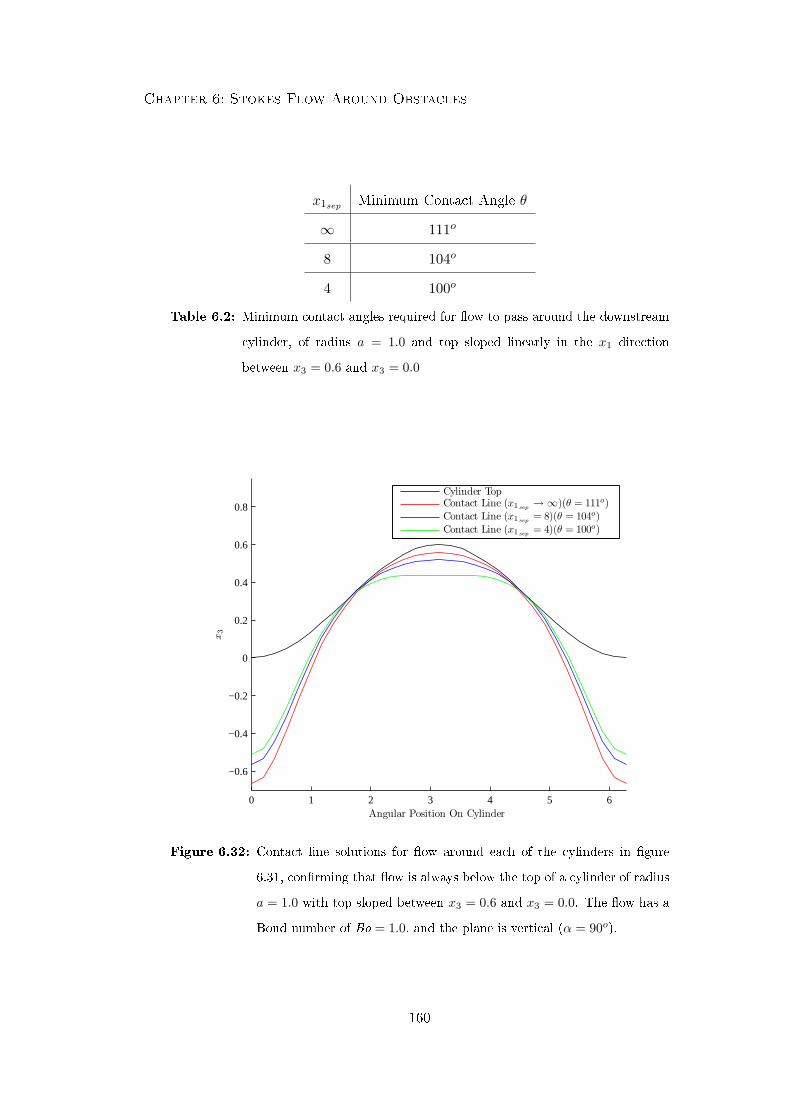
Chapter 6: Stokes Flow Around Obstacles
x1sep Minimum Contact Angle θ
∞ 111o
8 104o
4 100o
Table 6.2: Minimum contact angles required for ow to pass around the downstream
cylinder, of radius a = 1.0 and top sloped linearly in the x1 direction
between x3 = 0.6 and x3 = 0.0
0 1 2 3 4 5 6
−0.6
−0.4
−0.2
0
0.2
0.4
0.6
0.8
Angular Position On Cylinder
x3
Cylinder TopContact Line (x1sep → ∞)(θ = 111o)Contact Line (x1sep = 8)(θ = 104o)Contact Line (x1sep = 4)(θ = 100o)
Figure 6.32: Contact line solutions for ow around each of the cylinders in gure
6.31, conrming that ow is always below the top of a cylinder of radius
a = 1.0 with top sloped between x3 = 0.6 and x3 = 0.0. The ow has a
Bond number of Bo = 1.0, and the plane is vertical (α = 90o).
160

Chapter 6: Stokes Flow Around Obstacles
cylinders spaced by nite separations x1sep = 8 and 4. As the cylinders are moved closer
the proles over each obstacle interact more severely and the contact angle condition
necessary at the downstream cylinder is reduced.
Figure 6.32 illustrates the contact lines and cylinder top for the three scenarios for ow
around a cylinder depicted in gure 6.31. Clearly in each case the ow proles remain
below the cylinder top, and in general as the cylinders are brought closer together, a
attening of the highest region of the proles occurs.
161
Chapter 7
Small Inertial Eects Of Flow Over
And Around Obstacles
Film proles so far have been modelled using a Stokes ow approximation, and although
typical lm ows within a bearing chamber often have low Reynolds number, the eects of
the convective term may still be relevant regarding the free surface and velocity proles.
This chapter considers small inertial eects for lm ows both over and around circular
cylinders.
Section 7.1 overviews existing literature for the analysis of ows at low Reynolds num-
ber. Within this literature, the validation of numerical schemes is usually conducted
for ow in a lid-driven cavity. Due to the size of the three-dimensional lm domain,
an ecient numerical algorithm for evaluation of the convective term within the Navier
Stokes equations is required. Section 7.2 considers ow in a three-dimensional lid-driven
cavity for analysis of a computationally ecient numerical algorithm used to evaluate
low Reynolds number ows. Solutions to the Navier-Stokes equations are found via the
boundary element method (BEM) using an iterative technique. Conventional methods
linearly approximate the convective term and solve for domain velocities and unknown
boundary variables together. An alternative, more ecient approach where the convec-
tive term is evaluated directly from a previous estimate is considered, and the homoge-
neous and particular components of the ow are solved separately. In addition, to further
162
Chapter 7: Small Inertial Effects Of Flow Over And Around Obstacles
reduce the computational requirements of the ow problem, a local mass conservative in-
terpolation for the velocity eld is implemented. Section 7.3 considers the inertia eects
for lm ows over and around circular cylindrical obstacles, using the ecient numerical
algorithms developed for the case of a lid-driven cavity.
7.1 Literature Review
The boundary element method (BEM) is a well established technique for solving Stokes
ow problems. However diculties occur when extending the formulation to the non-
linear problem of nite Reynolds number ows. In these cases the integral representations
contain domain integrals caused by the convective term, and the evaluation of these
integrals is a major aspect of current research.
The domain integrals within the formulation can be solved eectively using techniques
such as nite dierence approximations (FDAs) and the nite element method (FEM).
However these methods result in the loss of the boundary-only nature of the formu-
lation. Methods have been developed which transform these domain integrals to the
boundary, for example the dual reciprocity method (DRM) and the particular integrals
technique (PIT) as developed by Nardini and Brebbia [43] and Ahmad and Banerjee [54]
respectively. In the latter method, solutions are decomposed into a homogeneous and
particular component satisfying the corresponding homogeneous and non-homogeneous
partial dierential equations (PDE). The particular solution fails to satisfy the bound-
ary conditions of the problem, and thus the boundary conditions of the homogeneous
PDE are modied to retain the original boundary conditions. The homogeneous PDE is
solved by the corresponding integral equation with these new boundary conditions ap-
plied. This particular solution concept is used within the DRM but instead of solving for
homogeneous and particular components separately, the domain integral is converted to
boundary integrals by use of the divergence theorem. As the non-homogeneous convective
term is unknown for this analysis, both the PIT and DRM approaches are numerically
163
Chapter 7: Small Inertial Effects Of Flow Over And Around Obstacles
equivalent.
The later work by Power and Botte [55] used a particular solution technique (PST)
to solve low Reynolds number ow in a lid driven cavity. The formulation is based
on the PIT approach, with the numerical procedure solving for the homogeneous and
particular components separately. In addition an indirect BEM is used for solution of
the homogeneous component. This PST method oered substantial benets to the DRM
and PIT models, reducing the computational cost of the numerical procedures.
When solving the Navier-Stokes equations, the nonlinear convective term requires accu-
rate values for the derivatives of the velocity eld. Conventional methods use a standard
interpolation for the velocities, from which the derivatives can be found. However, these
methods do not satisfy mass conservation causing inaccuracies, especially in regions of
coarse mesh, or high velocity gradients. Use of a mass conservative interpolation was
introduced by Florez and Power [56], and will be implemented throughout this chapter.
Solution of the Navier-Stokes equations using the DRM or other similar approaches often
results in numerical schemes that require excessive computational requirements. Specif-
ically, in cases where a mass conservative interpolation of the velocity eld is used, both
RAM and CPU time necessary to conduct the global radial basis function (RBF) in-
terpolation may become prohibitive. Thus a local mass conservative RBF interpolation
may be considered, with the possibility of signicantly reducing the computational re-
quirements. Local interpolations are discussed briey in chapter 3, and Yamada et al.
[57] show that despite the RBF interpolation being globally dened, it exhibits local
behaviour when reconstructing the approximated function.
Reducing the computational requirements necessary for nding ow proles at low
Reynolds number is a priority. Thus, for the case of three-dimensional lm ows at
low Reynolds number, the PST approach is implemented. The following section de-
velops the method for ow within a three-dimensional lid driven cavity with solutions
produced in an iterative fashion. Initially a global mass conservative RBF interpolation
164
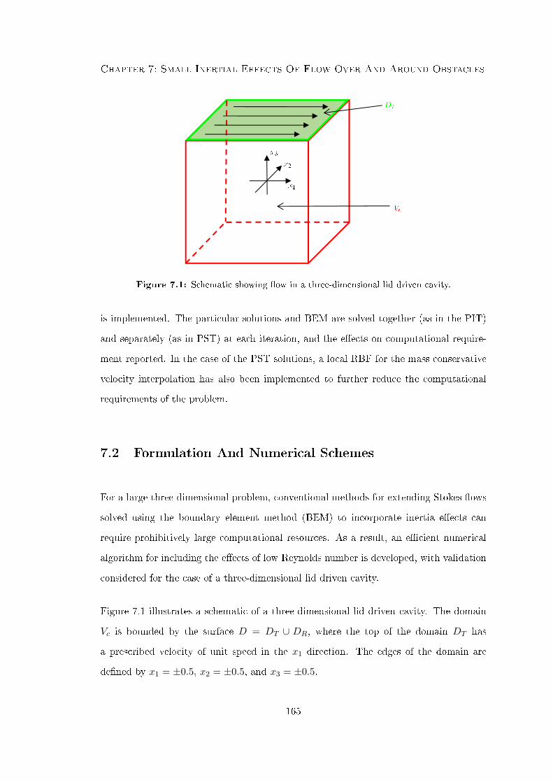
Chapter 7: Small Inertial Effects Of Flow Over And Around Obstacles
Figure 7.1: Schematic showing ow in a three-dimensional lid driven cavity.
is implemented. The particular solutions and BEM are solved together (as in the PIT)
and separately (as in PST) at each iteration, and the eects on computational require-
ment reported. In the case of the PST solutions, a local RBF for the mass conservative
velocity interpolation has also been implemented to further reduce the computational
requirements of the problem.
7.2 Formulation And Numerical Schemes
For a large three-dimensional problem, conventional methods for extending Stokes ows
solved using the boundary element method (BEM) to incorporate inertia eects can
require prohibitively large computational resources. As a result, an ecient numerical
algorithm for including the eects of low Reynolds number is developed, with validation
considered for the case of a three-dimensional lid driven cavity.
Figure 7.1 illustrates a schematic of a three-dimensional lid driven cavity. The domain
Vc is bounded by the surface D = DT ∪ DR, where the top of the domain DT has
a prescribed velocity of unit speed in the x1 direction. The edges of the domain are
dened by x1 = ±0.5, x2 = ±0.5, and x3 = ±0.5.
165

Chapter 7: Small Inertial Effects Of Flow Over And Around Obstacles
Flow within the cavity is governed by the usual incompressible equations for mass con-
tinuity (7.2.1) and Navier-Stokes (7.2.2),
∂ui∂xi
= 0, (7.2.1)
− ∂p
∂xi+∂2ui∂x2
j
= Re uj∂ui∂xj
, (7.2.2)
subject to the no slip boundary conditions
ui = δi1 x ∈ DT , (7.2.3)
ui = 0 x ∈ DR. (7.2.4)
The inclusion of the convective term within a boundary integral formulation can take
two forms, the dual reciprocity method [43] is rst considered in the following subsection.
The alternative homogeneous and particular solution approach [54] is then considered.
7.2.1 The Dual Reciprocity Method
The dual reciprocity method (DRM) as developed by Nardini and Brebbia [43] involves
formulating the integral equations for the Navier-Stokes equations, and converting the
domain integral for the convective term into boundary integrals. From the Lorentz
reciprocal relation in chapter 2
u′j∂σij∂xi− uj
∂σ′ij∂xi
=∂
∂xi(u′jσij − ujσ′ij). (7.2.5)
Set,
ui(x) =1
8πGim(x,x0)bm, (7.2.6)
σik(x) =1
8πTimj(x,x0)bm, (7.2.7)
as in chapter 2, but in this case
∂σij∂xi
= Bj = Re uk∂uj∂xk
, (7.2.8)
166
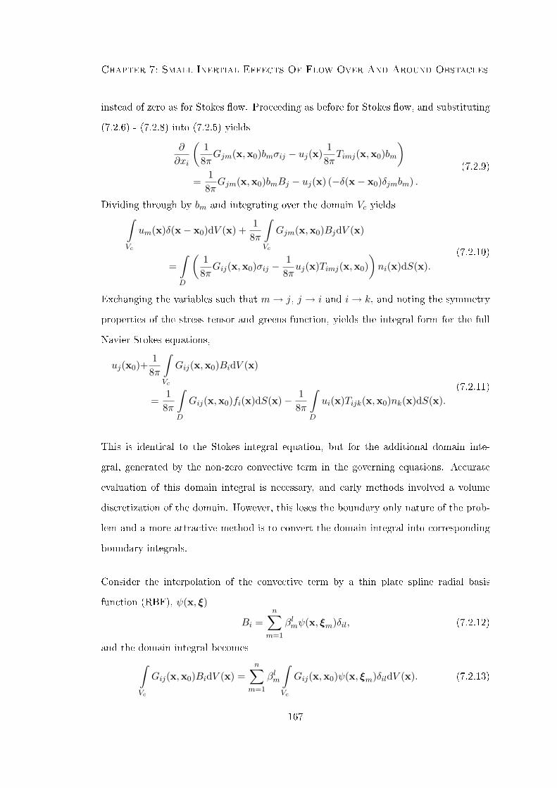
Chapter 7: Small Inertial Effects Of Flow Over And Around Obstacles
instead of zero as for Stokes ow. Proceeding as before for Stokes ow, and substituting
(7.2.6) - (7.2.8) into (7.2.5) yields
∂
∂xi
(1
8πGjm(x,x0)bmσij − uj(x)
18πTimj(x,x0)bm
)=
18πGjm(x,x0)bmBj − uj(x) (−δ(x− x0)δjmbm) .
(7.2.9)
Dividing through by bm and integrating over the domain Vc yields∫Vc
um(x)δ(x− x0)dV (x) +1
8π
∫Vc
Gjm(x,x0)BjdV (x)
=∫D
(1
8πGij(x,x0)σij −
18πuj(x)Timj(x,x0)
)ni(x)dS(x).
(7.2.10)
Exchanging the variables such that m→ j, j → i and i→ k, and noting the symmetry
properties of the stress tensor and greens function, yields the integral form for the full
Navier-Stokes equations,
uj(x0)+1
8π
∫Vc
Gij(x,x0)BidV (x)
=1
8π
∫D
Gij(x,x0)fi(x)dS(x)− 18π
∫D
ui(x)Tijk(x,x0)nk(x)dS(x).(7.2.11)
This is identical to the Stokes integral equation, but for the additional domain inte-
gral, generated by the non-zero convective term in the governing equations. Accurate
evaluation of this domain integral is necessary, and early methods involved a volume
discretization of the domain. However, this loses the boundary only nature of the prob-
lem and a more attractive method is to convert the domain integral into corresponding
boundary integrals.
Consider the interpolation of the convective term by a thin plate spline radial basis
function (RBF), ψ(x, ξ)
Bi =n∑
m=1
βlmψ(x, ξm)δil, (7.2.12)
and the domain integral becomes∫Vc
Gij(x,x0)BidV (x) =n∑
m=1
βlm
∫Vc
Gij(x,x0)ψ(x, ξm)δildV (x). (7.2.13)
167
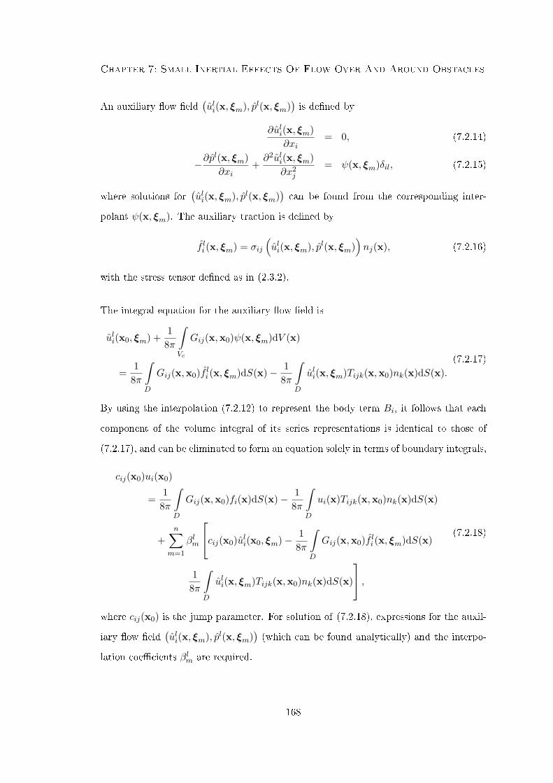
Chapter 7: Small Inertial Effects Of Flow Over And Around Obstacles
An auxiliary ow eld(uli(x, ξm), pl(x, ξm)
)is dened by
∂uli(x, ξm)∂xi
= 0, (7.2.14)
−∂pl(x, ξm)∂xi
+∂2uli(x, ξm)
∂x2j
= ψ(x, ξm)δil, (7.2.15)
where solutions for(uli(x, ξm), pl(x, ξm)
)can be found from the corresponding inter-
polant ψ(x, ξm). The auxiliary traction is dened by
f li (x, ξm) = σij
(uli(x, ξm), pl(x, ξm)
)nj(x), (7.2.16)
with the stress tensor dened as in (2.3.2).
The integral equation for the auxiliary ow eld is
uli(x0, ξm) +1
8π
∫Vc
Gij(x,x0)ψ(x, ξm)dV (x)
=1
8π
∫D
Gij(x,x0)f li (x, ξm)dS(x)− 18π
∫D
uli(x, ξm)Tijk(x,x0)nk(x)dS(x).(7.2.17)
By using the interpolation (7.2.12) to represent the body term Bi, it follows that each
component of the volume integral of its series representations is identical to those of
(7.2.17), and can be eliminated to form an equation solely in terms of boundary integrals,
cij(x0)ui(x0)
=1
8π
∫D
Gij(x,x0)fi(x)dS(x)− 18π
∫D
ui(x)Tijk(x,x0)nk(x)dS(x)
+n∑
m=1
βlm
cij(x0)uli(x0, ξm)− 18π
∫D
Gij(x,x0)f li (x, ξm)dS(x)
18π
∫D
uli(x, ξm)Tijk(x,x0)nk(x)dS(x)
,
(7.2.18)
where cij(x0) is the jump parameter. For solution of (7.2.18), expressions for the auxil-
iary ow eld(uli(x, ξm), pl(x, ξm)
)(which can be found analytically) and the interpo-
lation coecients βlm are required.
168
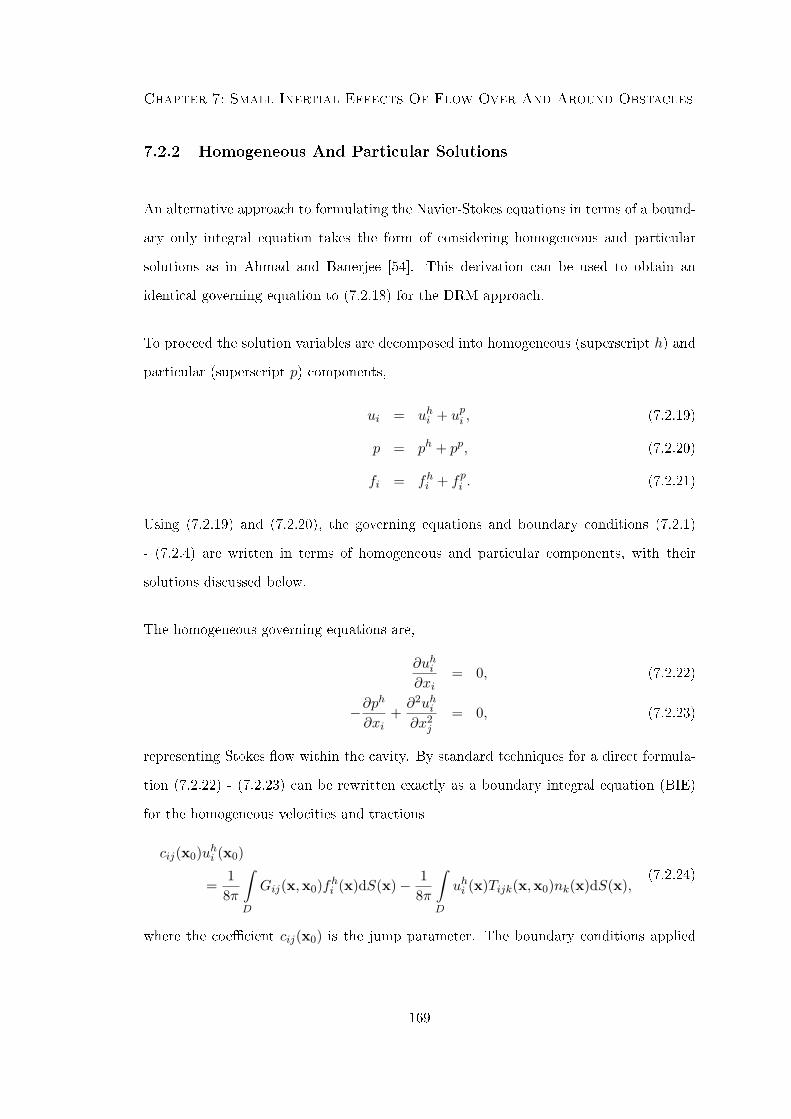
Chapter 7: Small Inertial Effects Of Flow Over And Around Obstacles
7.2.2 Homogeneous And Particular Solutions
An alternative approach to formulating the Navier-Stokes equations in terms of a bound-
ary only integral equation takes the form of considering homogeneous and particular
solutions as in Ahmad and Banerjee [54]. This derivation can be used to obtain an
identical governing equation to (7.2.18) for the DRM approach.
To proceed the solution variables are decomposed into homogeneous (superscript h) and
particular (superscript p) components,
ui = uhi + upi , (7.2.19)
p = ph + pp, (7.2.20)
fi = fhi + fpi . (7.2.21)
Using (7.2.19) and (7.2.20), the governing equations and boundary conditions (7.2.1)
- (7.2.4) are written in terms of homogeneous and particular components, with their
solutions discussed below.
The homogeneous governing equations are,
∂uhi∂xi
= 0, (7.2.22)
−∂ph
∂xi+∂2uhi∂x2
j
= 0, (7.2.23)
representing Stokes ow within the cavity. By standard techniques for a direct formula-
tion (7.2.22) - (7.2.23) can be rewritten exactly as a boundary integral equation (BIE)
for the homogeneous velocities and tractions
cij(x0)uhi (x0)
=1
8π
∫D
Gij(x,x0)fhi (x)dS(x)− 18π
∫D
uhi (x)Tijk(x,x0)nk(x)dS(x),(7.2.24)
where the coecient cij(x0) is the jump parameter. The boundary conditions applied
169
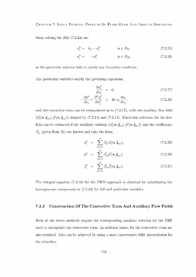
Chapter 7: Small Inertial Effects Of Flow Over And Around Obstacles
when solving the BIE (7.2.24) are
uhi = δi1 − upi x ∈ DT , (7.2.25)
uhi = −upi x ∈ DR, (7.2.26)
as the particular solution fails to satisfy any boundary condition.
The particular variables satisfy the governing equations,
∂upi∂xi
= 0, (7.2.27)
−∂pp
∂xi+∂2upi∂x2
j
= Re uj∂ui∂xj
, (7.2.28)
and the convective term can be interpolated as in (7.2.12), with the auxiliary ow eld(uli(x, ξm), pl(x, ξm)
)dened by (7.2.14) and (7.2.15). Particular solutions for the ow
eld can be evaluated if the auxiliary solution(uli(x, ξm), pl(x, ξm)
)and the coecients
βlm (given from Bi) are known and take the form,
upi =n∑
m=1
βlmuli(x, ξm), (7.2.29)
pp =n∑
m=1
βlmpl(x, ξm), (7.2.30)
fpi =n∑
m=1
βlmfli (x, ξm). (7.2.31)
The integral equation (7.2.18) for the DRM approach is obtained by substituting the
homogeneous components in (7.2.24) for full and particular variables.
7.2.3 Construction Of The Convective Term And Auxiliary Flow Fields
Both of the above methods require the corresponding auxiliary solution for the RBF
used to interpolate the convective term. In addition values for the convective term are
also required. This can be achieved by using a mass conservative RBF interpolation for
the velocities.
170

Chapter 7: Small Inertial Effects Of Flow Over And Around Obstacles
The convective term Bi is represented by interpolating the domain velocities with a RBF,
and then using this interpolation to evaluate the derivatives of the velocity eld. The
interpolation is further constrained to satisfy mass conservation, as considered by Florez
and Power [56]. A thin plate spline RBF of the form
ψ(x, ξ) = r3, (7.2.32)
is chosen, where r =‖ x− ξ ‖, and in this case a second order polynomial of the form
P2 = αP1 +αP2 x1 + αP3 x2 + αP4 x3 + αP5 x1x2
αP6 x1x3 + αP7 x2x3 + αP8 x21 + αP9 x
22 + αP10x
23,
(7.2.33)
is required to guarantee invertibility, along with the appropriate homogeneous constraint
condition.
The velocity eld is represented by the Hermitian interpolation shown below
u1 =n∑
m=1
α1mψ(x, ξm) +
n∑m=1
α4m
∂ψ(x, ξm)∂ξ1
+ P 12 , (7.2.34)
u2 =n∑
m=1
α2mψ(x, ξm) +
n∑m=1
α4m
∂ψ(x, ξm)∂ξ2
+ P 22 , (7.2.35)
u3 =n∑
m=1
α3mψ(x, ξm) +
n∑m=1
α4m
∂ψ(x, ξm)∂ξ3
+ P 32 . (7.2.36)
Corresponding derivatives of the velocity eld are found by,
∂ui∂xj
=n∑
m=1
αim∂ψ(x, ξm)
∂xj+
n∑m=1
α4m
∂ψ(x, ξm)∂ξi∂xj
+∂P i2∂xj
. (7.2.37)
The mass conservative formulation forms the matrix problem W3ijxj = bi, where the
rst three rows of the matrix W3ij in (7.2.38) consists of the velocity interpolations u1,
u2 and u3 as given by (7.2.34) - (7.2.36), collocated over n data points. The fourth
row satises ∂u1∂x1
+ ∂u2∂x2
+ ∂u3∂x3
= 0, corresponding to mass conservation and applied over
the same n data points as the velocity interpolation. The nal three rows describe the
homogeneous constraint condition, required to guarantee invertibility of the interpolation
171
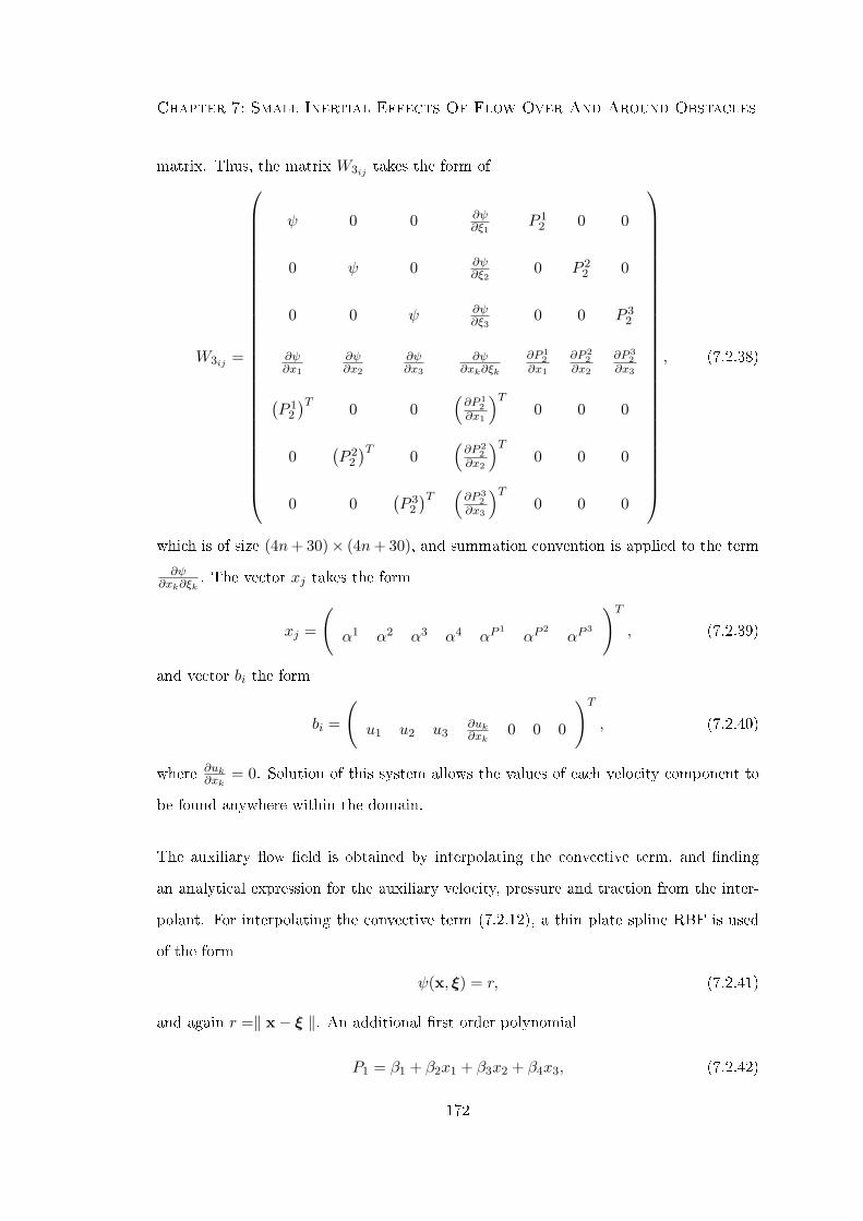
Chapter 7: Small Inertial Effects Of Flow Over And Around Obstacles
matrix. Thus, the matrix W3ij takes the form of
W3ij =
ψ 0 0 ∂ψ∂ξ1
P 12 0 0
0 ψ 0 ∂ψ∂ξ2
0 P 22 0
0 0 ψ ∂ψ∂ξ3
0 0 P 32
∂ψ∂x1
∂ψ∂x2
∂ψ∂x3
∂ψ∂xk∂ξk
∂P 12
∂x1
∂P 22
∂x2
∂P 32
∂x3(P 1
2
)T 0 0(∂P 1
2∂x1
)T0 0 0
0(P 2
2
)T 0(∂P 2
2∂x2
)T0 0 0
0 0(P 3
2
)T (∂P 3
2∂x3
)T0 0 0
, (7.2.38)
which is of size (4n+ 30)× (4n+ 30), and summation convention is applied to the term
∂ψ∂xk∂ξk
. The vector xj takes the form
xj =
(α1 α2 α3 α4 αP
1αP
2αP
3
)T, (7.2.39)
and vector bi the form
bi =
(u1 u2 u3
∂uk∂xk
0 0 0
)T, (7.2.40)
where ∂uk∂xk
= 0. Solution of this system allows the values of each velocity component to
be found anywhere within the domain.
The auxiliary ow eld is obtained by interpolating the convective term, and nding
an analytical expression for the auxiliary velocity, pressure and traction from the inter-
polant. For interpolating the convective term (7.2.12), a thin plate spline RBF is used
of the form
ψ(x, ξ) = r, (7.2.41)
and again r =‖ x− ξ ‖. An additional rst order polynomial
P1 = β1 + β2x1 + β3x2 + β4x3, (7.2.42)
172

Chapter 7: Small Inertial Effects Of Flow Over And Around Obstacles
along with a homogeneous constraint condition is necessary to guarantee invertibility
of the system. This interpolation of the convective term requires the solution of the
matrix-vector problem W1ijβ = bi where the matrix W1ij is given by
W1ij =
ψ P1
(P1)T 0
, (7.2.43)
of size (n+ 4)× (n+ 4), and the vector bi is
bi =
(B 0
)T. (7.2.44)
The auxiliary solutions to (7.2.14)and (7.2.15) are found by rst representing the solution
in terms of the potential φ(r),
uli(x, ξm) =∂2φ(r)∂x2
k
δil −∂2φ(r)∂xi∂xl
, (7.2.45)
which can be shown to satisfy conservation of mass (7.2.14). Substituting the expression
(7.2.45) for uli(x, ξm) into (7.2.15) yields
−∂pl(x, ξm)∂xi
+∂4φ(r)∂x4
k
δil −∂4φ(r)
∂xi∂xl∂x2k
= ψ(x, ξm)δil. (7.2.46)
The potential φ(r) is chosen to satisfy the non-homogeneous bi-harmonic equation
∂4φ(r)∂x4
k
= ψ(r), (7.2.47)
as the RBF can be written in terms of the radial distance, r. Correspondingly, the
auxiliary pressure is given by
pl(x, ξm) = − ∂3φ(r)
∂xl∂x2k
, (7.2.48)
and the traction is found by (7.2.16).
The potential φ(r) is found from equation (7.2.47), and the auxiliary velocity, pressure
and traction can be found from (7.2.45), (7.2.48) and (7.2.16) respectively. The potential
173

Chapter 7: Small Inertial Effects Of Flow Over And Around Obstacles
and auxiliary ow eld is also required for the rst order polynomial (7.2.42). In this
case, the data centre ξj is not relevant, and solutions are a function of the collocation
node xi only.
The auxiliary variables uli, pl, and f li corresponding to ψ = r, ψ = 1, ψ = x1, ψ = x2,
and ψ = x3 are presented in Appendix C. It should be noted that although both uli and
f li are required for lm ow analysis, when considering a lid driven cavity, it is solely the
velocity eld which is of interest. As such, the particular pressures and tractions of the
ow eld are not required.
7.2.4 Numerical Techniques For Solving Low Reynolds Flow In A Lid
Driven Cavity
Solution of the above formulations for the low Reynolds number ow in a lid driven
cavity can take a range of iterative procedures. The conventional PIT approach involves
writing the problem in a boundary only integral representation. The velocity eld from
the previous iteration is used to linearize the convective term and the numerical scheme
forms a large matrix problem, solved at each iteration for the velocity eld within the
domain, and unknown values on the domain boundary (in this case boundary tractions).
Details of the formulation are shown later.
Alternatively, the convective term can be approximated entirely from the previous it-
eration, and the particular solution evaluated explicitly. The boundary conditions of
the integral equation for the homogeneous components can be updated and the homoge-
neous solution found throughout the domain. Although this particular solution technique
(PST) as used by Power and Botte [55] is generally less convergent than the more tra-
ditional PIT, it is appealing due to the signicant reduction in computational resources
required. In addition, due to the simplication in explicitly nding the particular solu-
tion, it is possible to reduce the computational requirements of the mass conservative
interpolation of the velocities further by means of a local interpolation. Details of this
174

Chapter 7: Small Inertial Effects Of Flow Over And Around Obstacles
Bounding Point d1 d2 d3 d4 d5 d6 d7 d8
Bounding Value 0.7 0.3 0.2 0.15 0.1 0.05 0.02 0.01
Table 7.1: Boundary values used to determine which numerical integration approach
to implement for the case of a lid driven cavity.
method are also considered.
For all numerical schemes, the BEM is implemented with constant elements. In addition,
renement of the numerical integration in cases with near-point singularities consists of
a combination of the adaptive Gaussian integration algorithm and element subdivision
approach outlined in chapter 4, with bounding values modied to those shown in table
7.1
Conventional Particular Integral Technique (PIT)
Within the PIT, the homogeneous BIE can be written in terms of the full velocity
variables (7.2.19), yielding
cij(x0)ui(x0)
=1
8π
∫D
Gij(x,x0)fhi (x)dS(x)− 18π
∫D
ui(x)Tijk(x,x0)nk(x)dS(x)
+n∑
m=1
βlm
cij(x0)uli(x0, ξm) +1
8π
∫D
uli(x, ξm)Tijk(x,x0)nk(x)dS(x)
,(7.2.49)
in terms of the auxiliary velocities and it is left to nd an approximation for βlm.
The matrix vector notation for the coecients β is
β = W−11 B, (7.2.50)
where W1 is the interpolation matrix of the RBF (7.2.43). In addition the matrix vector
notation for the mass conservative velocity interpolation is
u = W3α, (7.2.51)
175

Chapter 7: Small Inertial Effects Of Flow Over And Around Obstacles
where W3 is the interpolation matrix (7.2.38) and the derivatives of the velocity are
dened by,
∂u∂xj
=∂W3
∂xjα. (7.2.52)
Using expression (7.2.52) coecients β are dened by,
β = W−11 Uj
∂W3
∂xjW−1
3 u, (7.2.53)
where the term Uj is a matrix with jth velocity component from the previous iteration on
the leading diagonal. Clearly in solving the BIE (7.2.49), a large system of equations is
produced covering all boundary and domain points, and requires solving at each iteration.
Ecient Implementation Of Particular Solution Techniques (PST)
Alternatively to the PIT method outlined above, a more computationally ecient PST
approach can be developed by evaluating the particular solutions based entirely on the
data from the previous iteration. The process is described in the following bullet points.
(i) Make an initial guess for the velocities within the domain, e.g. Stokes ow.
(ii) Calculate the mass conservative RBF interpolation for the domain velocities (7.2.38)
to nd the coecients α.
(iii) Using (7.2.37) nd the derivatives of the velocity eld and evaluate the convective
term B.
(iv) Using the convective term, interpolate using (7.2.12) to nd βlm.
(v) Particular velocities within the domain can be found and are given by (7.2.29).
(vi) The boundary conditions to the homogeneous solution are updated using the par-
ticular solutions.
176

Chapter 7: Small Inertial Effects Of Flow Over And Around Obstacles
(vii) The homogeneous solution is found using the BIE (7.2.24) for unknown boundary
values.
(viii) The BIE is then implemented to nd the homogeneous velocities within the domain.
(ix) The homogeneous and particular velocities are combined, convergence is tested and
the procedure is repeated from step (ii) if necessary.
The advantage of the PST over the conventional PIT is the reduction in computational
requirements. In the PIT a large system of equations is generated during each iter-
ation which then require solving. In this analysis a smaller system (based on either
the unknown boundary quantities or domain points) is formed. In addition, the ma-
trix components of this system are unchanged throughout the iterations. Thus a LUD
decomposition can be generated initially, and then used at each iteration to obtain the
solution with a modied right-hand-side to the matrix vector problem.
The computational requirements associated with the evaluation of the mass conservative
velocity interpolation (7.2.38) can be further reduced. The matrix is large and of size
(4n+ 30)× (4n+ 30), where n is the number of interpolation points within the domain.
By using a local RBF interpolation, the problem can be reduced to n matrices of size
(4nl + 30)× (4nl + 30), where nl is the number of local interpolation points and nl n.
Typically nl ∼ 30 for this analysis and the RBF interpolation is constructed from the
closest nl data points to the global point of interest. Further details of local RBF
interpolations are given in chapter 3
7.2.5 Flow Proles For A Lid Driven Cavity
This subsection considers solutions for ow in a three-dimensional lid driven cavity at a
selection of Reynolds numbers. As the boundary velocities to the domain are known, a
regular array of interpolation points are used throughout the domain and boundary for
177

Chapter 7: Small Inertial Effects Of Flow Over And Around Obstacles
the mass conservative velocity, and inertia interpolations. These interpolations are used
to nd the particular velocities at the collocation points of the BEM and the internal do-
main points. In all test cases 3456 triangular boundary elements and 2197 interpolation
points are used. Initially comparison of the PIT using a global mass conservative inter-
polation and the PST using both the global and local mass conservative interpolations
is made. Analysis for both the computational time and peak RAM requirements of the
formulations is conducted. The use of a local interpolation introduces an additional ap-
proximation in the analysis, and the accuracy of the local interpolation and the choice of
nl is considered. Following this analysis, results are presented for the three-dimensional
lid driven cavity, giving good agreement with previously published results.
Comparison Of Methods
The computational performance of the three numerical methods are compared when
solving for the velocity eld in a lid driven cavity at Re = 100. In all cases the iterative
loop requires an under-relaxation factor for convergence. For the PIT an under-relaxation
factor of 0.8 was found optimum; for the global PST, a value of 0.5 was used and for
the local PST, 0.6 was required. In each case the under-relaxation value was found
optimum to the nearest tenth. For the local interpolation, the number of points used
was minimized, whilst avoiding a singular interpolation matrix, and in this case 27 points
was found as the minimum. Figure 7.2 indicates the computational requirements of peak
RAM and run time for each numerical method. Clearly using the global PST over the
PIT produces signicant advantages in terms of computational resources required. The
RAM required reduces from 6.5GB to 4GB, and the run time is over 20 times faster.
Moving to the local RBF interpolation gives further reduction in computational resources
required. Peak RAM reduces to under 3.5GB, and the simulation time is halved again
from the global PST. Clearly a signicant reduction in the computational requirements
of the problem is made when adopting the PST over a more conventional PIT approach.
178
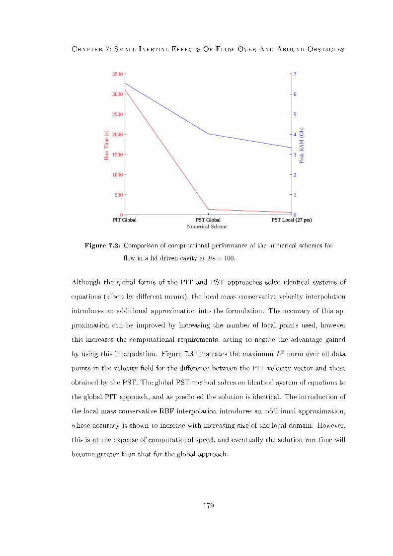
Chapter 7: Small Inertial Effects Of Flow Over And Around Obstacles
PIT Global PST Global PST Local (27 pts)0
500
1000
1500
2000
2500
3000
3500
Numerical Scheme
Run
Tim
e(s
)
PIT Global PST Global PST Local (27 pts)0
1
2
3
4
5
6
7
Pea
kRA
M(G
b)
Figure 7.2: Comparison of computational performance of the numerical schemes for
ow in a lid driven cavity at Re = 100.
Although the global forms of the PIT and PST approaches solve identical systems of
equations (albeit by dierent means), the local mass conservative velocity interpolation
introduces an additional approximation into the formulation. The accuracy of this ap-
proximation can be improved by increasing the number of local points used, however
this increases the computational requirements, acting to negate the advantage gained
by using this interpolation. Figure 7.3 illustrates the maximum L2 norm over all data
points in the velocity eld for the dierence between the PIT velocity vector and those
obtained by the PST. The global PST method solves an identical system of equations to
the global PIT approach, and as predicted the solution is identical. The introduction of
the local mass conservative RBF interpolation introduces an additional approximation,
whose accuracy is shown to increase with increasing size of the local domain. However,
this is at the expense of computational speed, and eventually the solution run time will
become greater than that for the global approach.
179
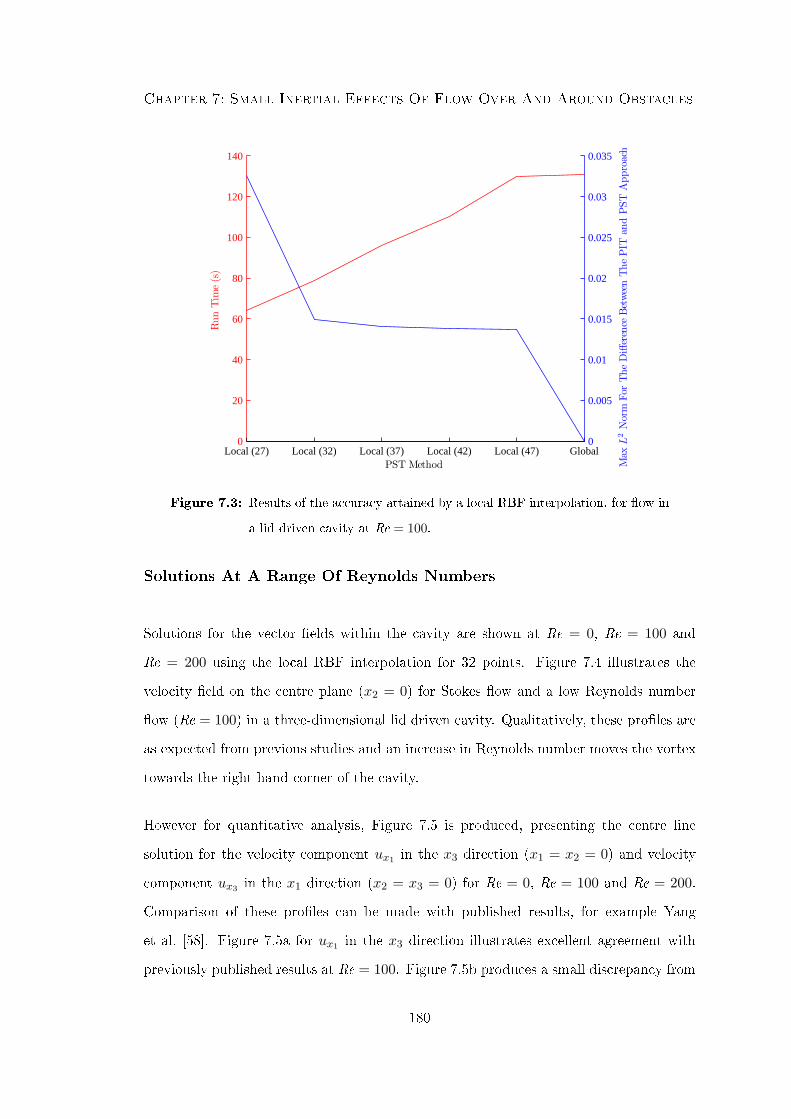
Chapter 7: Small Inertial Effects Of Flow Over And Around Obstacles
Local (27) Local (32) Local (37) Local (42) Local (47) Global0
20
40
60
80
100
120
140
PST Method
Run
Tim
e(s
)
0
0.005
0.01
0.015
0.02
0.025
0.03
0.035
Max
L2
Nor
mFo
rThe
Diff
eren
ceBet
wee
nThe
PIT
and
PST
App
roac
h
Figure 7.3: Results of the accuracy attained by a local RBF interpolation, for ow in
a lid driven cavity at Re = 100.
Solutions At A Range Of Reynolds Numbers
Solutions for the vector elds within the cavity are shown at Re = 0, Re = 100 and
Re = 200 using the local RBF interpolation for 32 points. Figure 7.4 illustrates the
velocity eld on the centre plane (x2 = 0) for Stokes ow and a low Reynolds number
ow (Re = 100) in a three-dimensional lid driven cavity. Qualitatively, these proles are
as expected from previous studies and an increase in Reynolds number moves the vortex
towards the right hand corner of the cavity.
However for quantitative analysis, Figure 7.5 is produced, presenting the centre line
solution for the velocity component ux1 in the x3 direction (x1 = x2 = 0) and velocity
component ux3 in the x1 direction (x2 = x3 = 0) for Re = 0, Re = 100 and Re = 200.
Comparison of these proles can be made with published results, for example Yang
et al. [58]. Figure 7.5a for ux1 in the x3 direction illustrates excellent agreement with
previously published results at Re = 100. Figure 7.5b produces a small discrepancy from
180

Chapter 7: Small Inertial Effects Of Flow Over And Around Obstacles
−0.5 −0.4 −0.3 −0.2 −0.1 0 0.1 0.2 0.3 0.4 0.5−0.5
−0.4
−0.3
−0.2
−0.1
0
0.1
0.2
0.3
0.4
0.5(b)
x1(x2 = 0)
x3
−0.5 −0.4 −0.3 −0.2 −0.1 0 0.1 0.2 0.3 0.4 0.5−0.5
−0.4
−0.3
−0.2
−0.1
0
0.1
0.2
0.3
0.4
0.5(a)
x1(x2 = 0)
x3
Figure 7.4: Centre plane solution of ow in a three-dimensional lid driven cavity for
(a) Stokes ow (Re = 0) and (b) Re = 100.
181

Chapter 7: Small Inertial Effects Of Flow Over And Around Obstacles
published results for ux3 in the x1 direction at Re = 100. Here the prediction for the
vertical velocity is slightly greater between −0.2 < x1 < 0.4 than the equivalent prole
in [58].
7.3 Low Reynolds Number Film Flows
This section considers the inertial eects on ows over and around circular cylinders
at low Reynolds number. An overview of the mathematical formulation for the case of
lm ow at nite Reynolds number is initially presented. Following this, a numerical
approach is developed based on the optimal scheme developed for a three-dimensional lid
driven cavity in § 7.2. Finally results are presented indicating the eects of low Reynolds
number on the lm prole generated.
7.3.1 Formulation Of Low Reynolds Number Film Flows
The mathematical formulation is presented for lm ow down an inclined plane and
around an obstacle at nite Reynolds number. However, the formulation can be reduced
to ow over a single cylinder by omission of the contact line condition and the dry top
of the cylinder Sf . Figure 7.6 indicates a schematic for ow around a cylinder. This is
similar to that presented in gure 6.2, with the edges of the domain now marked as Se.
The ow is governed by mass continuity (7.3.1) and Navier-Stokes equation (7.3.2),
∂ui∂xi
= 0, (7.3.1)
− ∂p
∂xi+∂G
∂xi+∂2ui∂x2
j
= Re uj∂ui∂xj
, (7.3.2)
where G = −2(x3 cotα − x1) is the gravitational driving components as in the Stokes
case considered previously. A summary of the various surfaces dened in gure 7.6 are
given in table 7.2. By using the characteristic scales dened in table 4.1, the following
182

Chapter 7: Small Inertial Effects Of Flow Over And Around Obstacles
−0.4 −0.2 0 0.2 0.4 0.6 0.8 1−0.5
−0.4
−0.3
−0.2
−0.1
0
0.1
0.2
0.3
0.4
0.5(a)
ux1
x3(x
1=
x2
=0)
−0.5 −0.4 −0.3 −0.2 −0.1 0 0.1 0.2 0.3 0.4 0.5−0.25
−0.2
−0.15
−0.1
−0.05
0
0.05
0.1
0.15
0.2(b)
x1(x2 = x3 = 0)
ux3
Re = 0Re = 100Re = 200
Figure 7.5: Centre line solution at Re = 0, Re = 100 and Re = 200 for ow in a
three-dimensional lid driven cavity showing (a) velocity component ux1
in the x3 direction (x1 = x2 = 0) and (b) velocity component ux3 in the
x1 direction (x2 = x3 = 0).
183

Chapter 7: Small Inertial Effects Of Flow Over And Around Obstacles
Figure 7.6: Schematic showing nomenclature for ow around a cylinder at nite
Reynolds number. In this case the edges of the domain are denoted Se.
Sf Free surface
Sf Cylinder top
Sp Wetted cylinder surface
Se Edges to the domain
Sw Wall
Table 7.2: Denition of surface nomenclature.
expression for the Reynolds number can be found,
Re =H3g sinα
2ν2. (7.3.3)
The lm ow is subject to the following boundary conditions
ui = 0 x ∈ Sw, Sp, (7.3.4)
∂xi∂t
ni = ujnj x ∈ Sf , (7.3.5)
fi = − 4Bo
κni x ∈ Sf , (7.3.6)
∂h
∂xini = tan
(π2− θ)
x ∈ Sf ∩ Sp. (7.3.7)
No slip on the wall and wetted obstacle surface is dened by (7.3.4), the kinematic and
dynamic condition are dened by (7.3.5) - (7.3.6) respectively and applied on the free
surface. Finally, (7.3.7) is the contact line constraint.
184
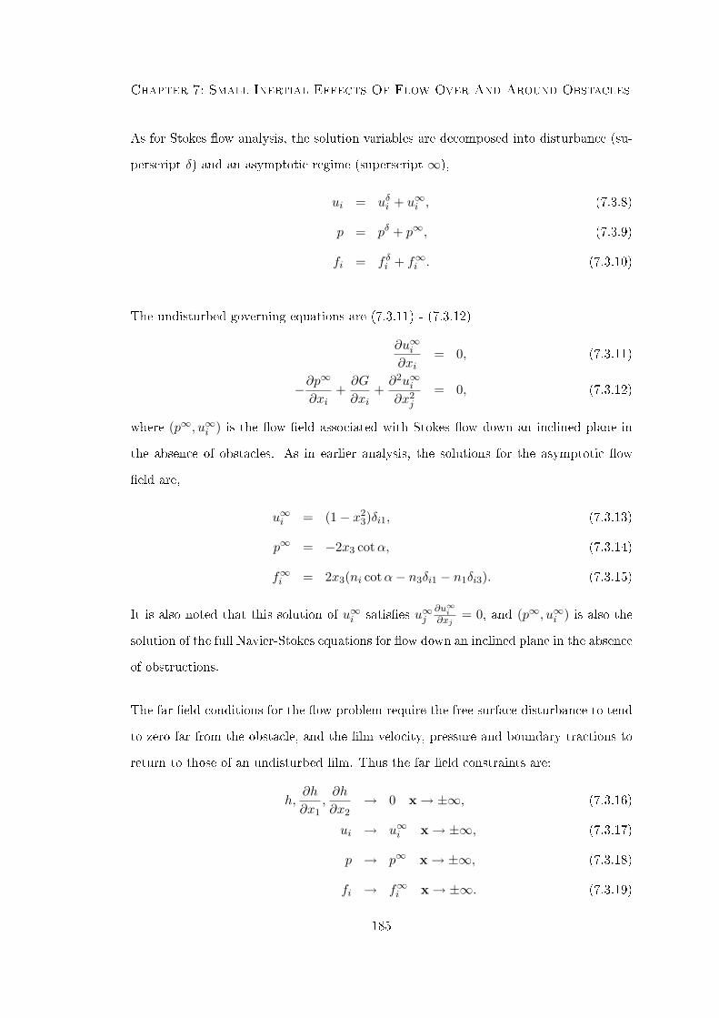
Chapter 7: Small Inertial Effects Of Flow Over And Around Obstacles
As for Stokes ow analysis, the solution variables are decomposed into disturbance (su-
perscript δ) and an asymptotic regime (superscript ∞),
ui = uδi + u∞i , (7.3.8)
p = pδ + p∞, (7.3.9)
fi = f δi + f∞i . (7.3.10)
The undisturbed governing equations are (7.3.11) - (7.3.12)
∂u∞i∂xi
= 0, (7.3.11)
−∂p∞
∂xi+∂G
∂xi+∂2u∞i∂x2
j
= 0, (7.3.12)
where (p∞, u∞i ) is the ow eld associated with Stokes ow down an inclined plane in
the absence of obstacles. As in earlier analysis, the solutions for the asymptotic ow
eld are,
u∞i = (1− x23)δi1, (7.3.13)
p∞ = −2x3 cotα, (7.3.14)
f∞i = 2x3(ni cotα− n3δi1 − n1δi3). (7.3.15)
It is also noted that this solution of u∞i satises u∞j∂u∞i∂xj
= 0, and (p∞, u∞i ) is also the
solution of the full Navier-Stokes equations for ow down an inclined plane in the absence
of obstructions.
The far eld conditions for the ow problem require the free surface disturbance to tend
to zero far from the obstacle, and the lm velocity, pressure and boundary tractions to
return to those of an undisturbed lm. Thus the far eld constraints are:
h,∂h
∂x1,∂h
∂x2→ 0 x→ ±∞, (7.3.16)
ui → u∞i x→ ±∞, (7.3.17)
p → p∞ x→ ±∞, (7.3.18)
fi → f∞i x→ ±∞. (7.3.19)
185
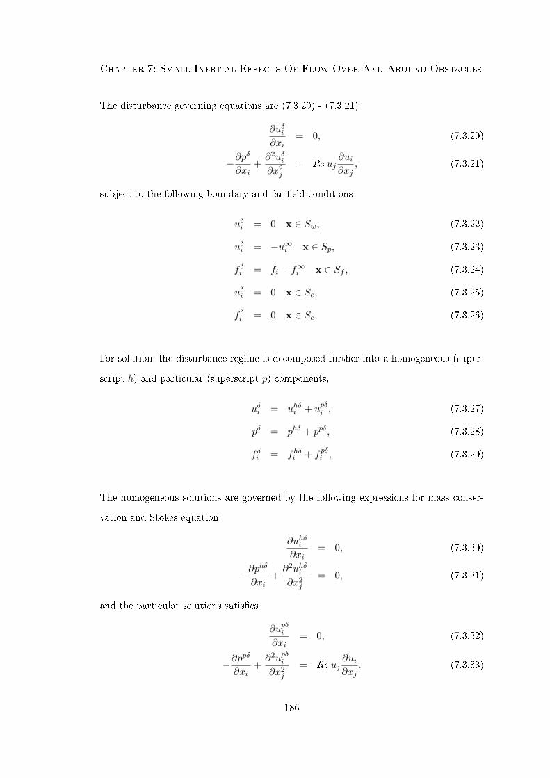
Chapter 7: Small Inertial Effects Of Flow Over And Around Obstacles
The disturbance governing equations are (7.3.20) - (7.3.21)
∂uδi∂xi
= 0, (7.3.20)
−∂pδ
∂xi+∂2uδi∂x2
j
= Re uj∂ui∂xj
, (7.3.21)
subject to the following boundary and far eld conditions
uδi = 0 x ∈ Sw, (7.3.22)
uδi = −u∞i x ∈ Sp, (7.3.23)
f δi = fi − f∞i x ∈ Sf , (7.3.24)
uδi = 0 x ∈ Se, (7.3.25)
f δi = 0 x ∈ Se, (7.3.26)
For solution, the disturbance regime is decomposed further into a homogeneous (super-
script h) and particular (superscript p) components,
uδi = uhδi + upδi , (7.3.27)
pδ = phδ + ppδ, (7.3.28)
f δi = fhδi + fpδi , (7.3.29)
The homogeneous solutions are governed by the following expressions for mass conser-
vation and Stokes equation
∂uhδi∂xi
= 0, (7.3.30)
−∂phδ
∂xi+∂2uhδi∂x2
j
= 0, (7.3.31)
and the particular solutions satises
∂upδi∂xi
= 0, (7.3.32)
−∂ppδ
∂xi+∂2upδi∂x2
j
= Re uj∂ui∂xj
. (7.3.33)
186
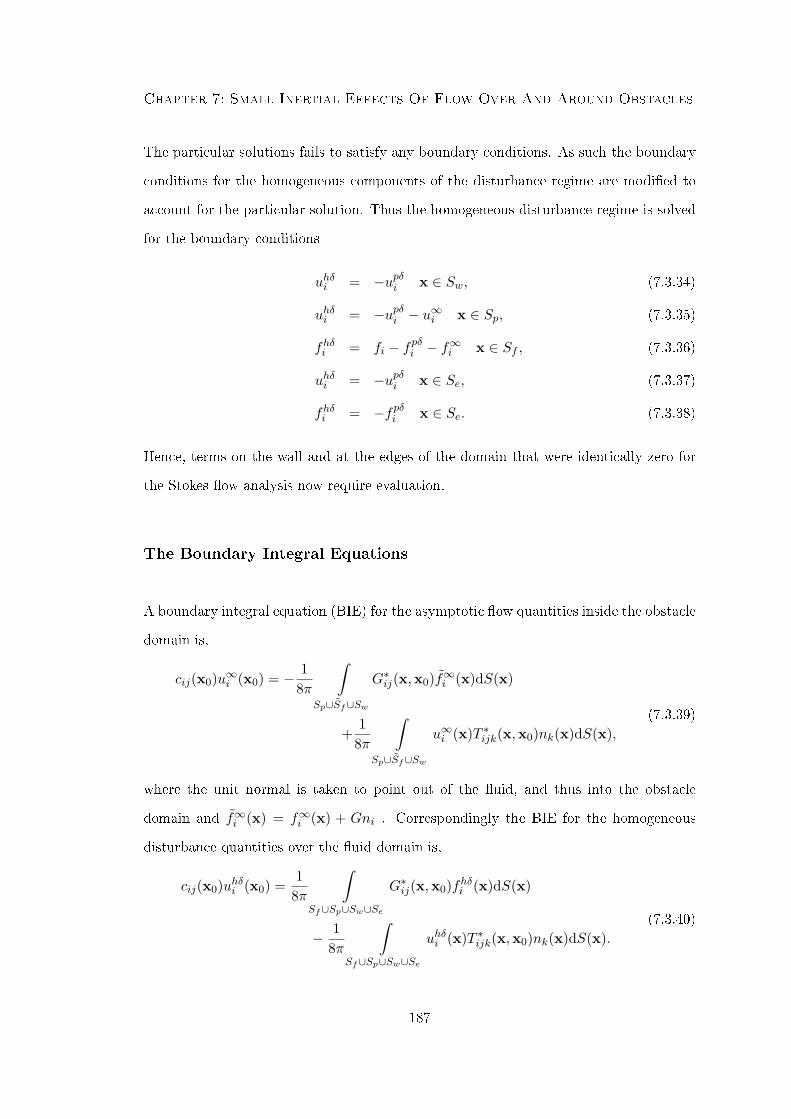
Chapter 7: Small Inertial Effects Of Flow Over And Around Obstacles
The particular solutions fails to satisfy any boundary conditions. As such the boundary
conditions for the homogeneous components of the disturbance regime are modied to
account for the particular solution. Thus the homogeneous disturbance regime is solved
for the boundary conditions
uhδi = −upδi x ∈ Sw, (7.3.34)
uhδi = −upδi − u∞i x ∈ Sp, (7.3.35)
fhδi = fi − fpδi − f∞i x ∈ Sf , (7.3.36)
uhδi = −upδi x ∈ Se, (7.3.37)
fhδi = −fpδi x ∈ Se. (7.3.38)
Hence, terms on the wall and at the edges of the domain that were identically zero for
the Stokes ow analysis now require evaluation.
The Boundary Integral Equations
A boundary integral equation (BIE) for the asymptotic ow quantities inside the obstacle
domain is,
cij(x0)u∞i (x0) = − 18π
∫Sp∪Sf∪Sw
G∗ij(x,x0)f∞i (x)dS(x)
+1
8π
∫Sp∪Sf∪Sw
u∞i (x)T ∗ijk(x,x0)nk(x)dS(x),(7.3.39)
where the unit normal is taken to point out of the uid, and thus into the obstacle
domain and f∞i (x) = f∞i (x) + Gni . Correspondingly the BIE for the homogeneous
disturbance quantities over the uid domain is,
cij(x0)uhδi (x0) =1
8π
∫Sf∪Sp∪Sw∪Se
G∗ij(x,x0)fhδi (x)dS(x)
− 18π
∫Sf∪Sp∪Sw∪Se
uhδi (x)T ∗ijk(x,x0)nk(x)dS(x).(7.3.40)
187

Chapter 7: Small Inertial Effects Of Flow Over And Around Obstacles
The Lorentz-Blake Green's functions yield G∗ij(x,x0) = 0 x ∈ Sw and also for the
asymptotic solution u∞i = 0 x ∈ Sw. Thus equations (7.3.39) and (7.3.40) become
cij(x0)u∞i (x0) = − 18π
∫Sp∪Sf
G∗ij(x,x0)f∞i (x)dS(x)
+1
8π
∫Sp∪Sf
u∞i (x)T ∗ijk(x,x0)nk(x)dS(x),(7.3.41)
and
cij(x0)uhδi (x0) =1
8π
∫Sf∪Sp∪Se
G∗ij(x,x0)fhδi (x)dS(x)
− 18π
∫Sf∪Sp∪Sw∪Se
uhδi (x)T ∗ijk(x,x0)nk(x)dS(x),(7.3.42)
respectively.
Collocation Over The Free Surface
When collocating over the free surface, the BIE for the asymptotic ow regime within
the obstacle becomes
18π
∫Sp∪Sf
G∗ij(x,x0)f∞i (x)dS(x)
=1
8π
∫Sp∪Sf
u∞i (x)T ∗ijk(x,x0)nk(x)dS(x),(7.3.43)
and the disturbance BIE becomes
12uhδj (x0) +
18π
∫Sf
uhδi (x)T ∗ijk(x,x0)nk(x)dS(x)
=1
8π
∫Sf
G∗ij(x,x0)fhδi (x)dS(x) +1
8π
∫Sp∪Se
G∗ij(x,x0)fhδi (x)dS(x)
− 18π
∫Sp∪Sw∪Se
uhδi (x)T ∗ijk(x,x0)nk(x)dS(x).
(7.3.44)
188
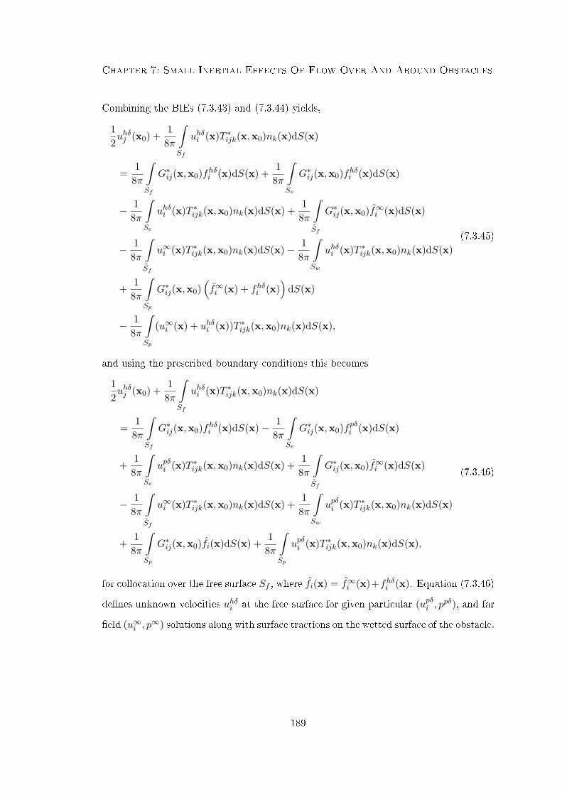
Chapter 7: Small Inertial Effects Of Flow Over And Around Obstacles
Combining the BIEs (7.3.43) and (7.3.44) yields,
12uhδj (x0) +
18π
∫Sf
uhδi (x)T ∗ijk(x,x0)nk(x)dS(x)
=1
8π
∫Sf
G∗ij(x,x0)fhδi (x)dS(x) +1
8π
∫Se
G∗ij(x,x0)fhδi (x)dS(x)
− 18π
∫Se
uhδi (x)T ∗ijk(x,x0)nk(x)dS(x) +1
8π
∫Sf
G∗ij(x,x0)f∞i (x)dS(x)
− 18π
∫Sf
u∞i (x)T ∗ijk(x,x0)nk(x)dS(x)− 18π
∫Sw
uhδi (x)T ∗ijk(x,x0)nk(x)dS(x)
+1
8π
∫Sp
G∗ij(x,x0)(f∞i (x) + fhδi (x)
)dS(x)
− 18π
∫Sp
(u∞i (x) + uhδi (x))T ∗ijk(x,x0)nk(x)dS(x),
(7.3.45)
and using the prescribed boundary conditions this becomes
12uhδj (x0) +
18π
∫Sf
uhδi (x)T ∗ijk(x,x0)nk(x)dS(x)
=1
8π
∫Sf
G∗ij(x,x0)fhδi (x)dS(x)− 18π
∫Se
G∗ij(x,x0)fpδi (x)dS(x)
+1
8π
∫Se
upδi (x)T ∗ijk(x,x0)nk(x)dS(x) +1
8π
∫Sf
G∗ij(x,x0)f∞i (x)dS(x)
− 18π
∫Sf
u∞i (x)T ∗ijk(x,x0)nk(x)dS(x) +1
8π
∫Sw
upδi (x)T ∗ijk(x,x0)nk(x)dS(x)
+1
8π
∫Sp
G∗ij(x,x0)fi(x)dS(x) +1
8π
∫Sp
upδi (x)T ∗ijk(x,x0)nk(x)dS(x),
(7.3.46)
for collocation over the free surface Sf , where fi(x) = f∞i (x)+fhδi (x). Equation (7.3.46)
denes unknown velocities uhδi at the free surface for given particular (upδi , ppδ), and far
eld (u∞i , p∞) solutions along with surface tractions on the wetted surface of the obstacle.
189

Chapter 7: Small Inertial Effects Of Flow Over And Around Obstacles
Collocation Over The Wetted Obstacle Surface
For collocation over the wetted obstacle surface, the BIE corresponding to the asymptotic
regime over the obstacle domain takes the form
12u∞j (x0) = − 1
8π
∫Sp∪Sf
G∗ij(x,x0)f∞i (x)dS(x)
+1
8π
∫Sp∪Sf
u∞i (x)T ∗ijk(x,x0)nk(x)dS(x),(7.3.47)
and the disturbance BIE the form
12uhδj (x0) =
18π
∫Sf
G∗ij(x,x0)fhδi (x)dS(x)
− 18π
∫Sf
uhδi (x)T ∗ijk(x,x0)nk(x)dS(x) +1
8π
∫Sp∪Se
G∗ij(x,x0)fhδi (x)dS(x)
− 18π
∫Sp∪Sw∪Se
uhδi (x)T ∗ijk(x,x0)nk(x)dS(x).
(7.3.48)
Rearranging (7.3.47) and (7.3.48) for the obstacle tractions, and combining yields
18π
∫Sp
G∗ij(x,x0)(f∞i (x) + fhδi (x)
)dS(x) =
12uhδj (x0)− 1
2u∞j (x0)
− 18π
∫Sf
G∗ij(x,x0)fhδi (x)dS(x) +1
8π
∫Sf
uhδi (x)T ∗ijk(x,x0)nk(x)dS(x)
− 18π
∫Se
G∗ij(x,x0)fhδi (x)dS(x) +1
8π
∫Se
uhδi (x)T ∗ijk(x,x0)nk(x)dS(x)
− 18π
∫Sf
G∗ij(x,x0)f∞i (x)dS(x) +1
8π
∫Sf
u∞i (x)T ∗ijk(x,x0)nk(x)dS(x)
+1
8π
∫Sw
uhδi (x)T ∗ijk(x,x0)nk(x)dS(x)
+1
8π
∫Sp
(uhδi (x) + u∞i (x))T ∗ijk(x,x0)nk(x)dS(x),
(7.3.49)
190
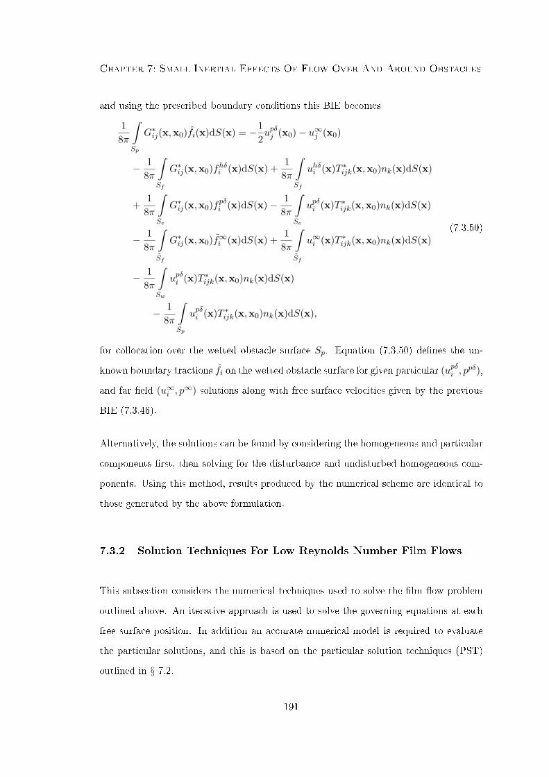
Chapter 7: Small Inertial Effects Of Flow Over And Around Obstacles
and using the prescribed boundary conditions this BIE becomes
18π
∫Sp
G∗ij(x,x0)fi(x)dS(x) = −12upδj (x0)− u∞j (x0)
− 18π
∫Sf
G∗ij(x,x0)fhδi (x)dS(x) +1
8π
∫Sf
uhδi (x)T ∗ijk(x,x0)nk(x)dS(x)
+1
8π
∫Se
G∗ij(x,x0)fpδi (x)dS(x)− 18π
∫Se
upδi (x)T ∗ijk(x,x0)nk(x)dS(x)
− 18π
∫Sf
G∗ij(x,x0)f∞i (x)dS(x) +1
8π
∫Sf
u∞i (x)T ∗ijk(x,x0)nk(x)dS(x)
− 18π
∫Sw
upδi (x)T ∗ijk(x,x0)nk(x)dS(x)
− 18π
∫Sp
upδi (x)T ∗ijk(x,x0)nk(x)dS(x),
(7.3.50)
for collocation over the wetted obstacle surface Sp. Equation (7.3.50) denes the un-
known boundary tractions fi on the wetted obstacle surface for given particular (upδi , ppδ),
and far eld (u∞i , p∞) solutions along with free surface velocities given by the previous
BIE (7.3.46).
Alternatively, the solutions can be found by considering the homogeneous and particular
components rst, then solving for the disturbance and undisturbed homogeneous com-
ponents. Using this method, results produced by the numerical scheme are identical to
those generated by the above formulation.
7.3.2 Solution Techniques For Low Reynolds Number Film Flows
This subsection considers the numerical techniques used to solve the lm ow problem
outlined above. An iterative approach is used to solve the governing equations at each
free surface position. In addition an accurate numerical model is required to evaluate
the particular solutions, and this is based on the particular solution techniques (PST)
outlined in § 7.2.
191
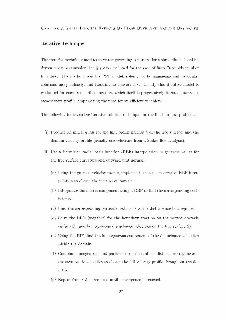
Chapter 7: Small Inertial Effects Of Flow Over And Around Obstacles
Iterative Technique
The iterative technique used to solve the governing equations for a three-dimensional lid
driven cavity as considered in § 7.2 is developed for the case of nite Reynolds number
lm ow. The method uses the PST model, solving for homogeneous and particular
solutions independently, and iterating to convergence. Clearly this iterative model is
evaluated for each free surface location, which itself is progressively iterated towards a
steady state prole, emphasizing the need for an ecient technique.
The following indicates the iterative solution technique for the full lm ow problem.
(i) Produce an initial guess for the lm prole heights h of the free surface, and the
domain velocity prole (usually use velocities from a Stokes ow analysis).
(ii) Use a Hermitian radial basis function (RBF) interpolation to generate values for
the free surface curvature and outward unit normal.
(a) Using the guessed velocity prole, implement a mass conservative RBF inter-
polation to obtain the inertia component.
(b) Interpolate the inertia component using a RBF to nd the corresponding coef-
cients.
(c) Find the corresponding particular solutions to the disturbance ow regime.
(d) Solve the BIEs (together) for the boundary traction on the wetted obstacle
surface Sp, and homogeneous disturbance velocities on the free surface Sf .
(e) Using the BIE, nd the homogeneous component of the disturbance velocities
within the domain.
(f) Combine homogeneous and particular solutions of the disturbance regime and
the asymptotic velocities to obtain the full velocity prole throughout the do-
main.
(g) Repeat from (a) as required until convergence is reached.
192

Chapter 7: Small Inertial Effects Of Flow Over And Around Obstacles
(iii) Use the converged velocity prole to update the free surface prole.
(iv) If the movement of the free surface is suciently small, then a steady-state prole
is found, alternative repeat from step (ii), using the new free surface location. In
addition, the initial guess for the domain velocities is made by a mass conservative
velocity interpolation, based on the converged velocities at the end of the previous
free surface iteration.
A key dierence to the Stokes ow analysis in earlier chapters, is that the BIEs are
solved together during the PST iteration, where previously the two BIEs have been
solved separately. This improves the convergence of the PST method.
The Boundary Element Method
The boundary element method (BEM) is applied similarly to the Stokes ow case to
evaluate the boundary integrals in (7.3.46) and (7.3.50), using constant functional, at
triangular elements throughout. However, four extra integrals are present when com-
pared to the Stokes case. These are,
(i) The double-layer potential over the wetted obstacle surface Sp.
(ii) The double-layer potential over the wall (external to the obstacle) Sw.
(iii) The single-layer potential over the edges of the domain Se.
(iv) The double-layer potential over the edges of the domain Se.
Point (i) above is simple to incorporate as the obstacle mesh is already discretized to
evaluate the single-layer potential. However, point (ii) above requires a mesh for the
wall, outside of the obstacle footprint, and points (iii) - (iv) need a mesh for the edges
of the domain. The x1x2 distribution of elements for the wall discretization are identical
193
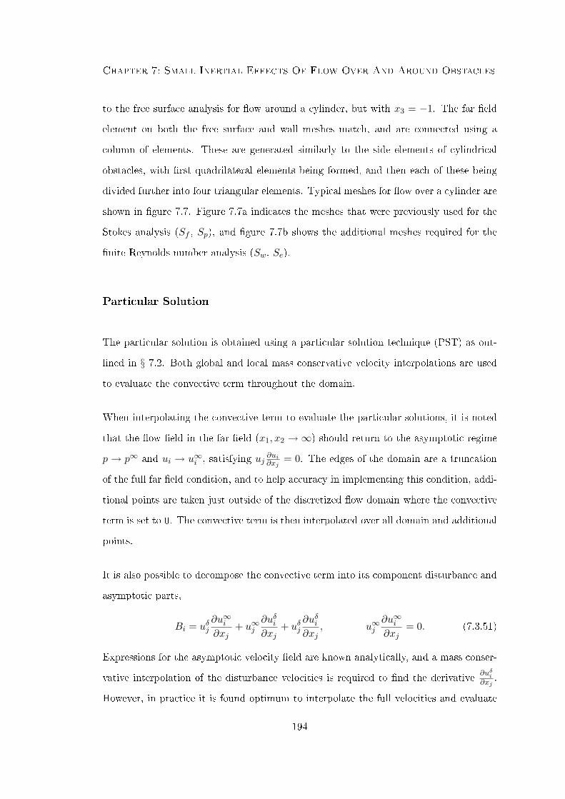
Chapter 7: Small Inertial Effects Of Flow Over And Around Obstacles
to the free surface analysis for ow around a cylinder, but with x3 = −1. The far eld
element on both the free surface and wall meshes match, and are connected using a
column of elements. These are generated similarly to the side elements of cylindrical
obstacles, with rst quadrilateral elements being formed, and then each of these being
divided further into four triangular elements. Typical meshes for ow over a cylinder are
shown in gure 7.7. Figure 7.7a indicates the meshes that were previously used for the
Stokes analysis (Sf , Sp), and gure 7.7b shows the additional meshes required for the
nite Reynolds number analysis (Sw, Se).
Particular Solution
The particular solution is obtained using a particular solution technique (PST) as out-
lined in § 7.2. Both global and local mass conservative velocity interpolations are used
to evaluate the convective term throughout the domain.
When interpolating the convective term to evaluate the particular solutions, it is noted
that the ow eld in the far eld (x1, x2 →∞) should return to the asymptotic regime
p → p∞ and ui → u∞i , satisfying uj∂ui∂xj
= 0. The edges of the domain are a truncation
of the full far eld condition, and to help accuracy in implementing this condition, addi-
tional points are taken just outside of the discretized ow domain where the convective
term is set to 0. The convective term is then interpolated over all domain and additional
points.
It is also possible to decompose the convective term into its component disturbance and
asymptotic parts,
Bi = uδj∂u∞i∂xj
+ u∞j∂uδi∂xj
+ uδj∂uδi∂xj
, u∞j∂u∞i∂xj
= 0. (7.3.51)
Expressions for the asymptotic velocity eld are known analytically, and a mass conser-
vative interpolation of the disturbance velocities is required to nd the derivative∂uδi∂xj
.
However, in practice it is found optimum to interpolate the full velocities and evaluate
194

Chapter 7: Small Inertial Effects Of Flow Over And Around Obstacles
−6 −4 −2 0 2 4 6 8−5
0
5−1
−0.5
0
0.5
x2
(a)
x1
x3
−6
−4
−2
0
2
4
6
8 −6
−4
−2
0
2
4
6
−1
−0.5
0
x2
(b)
x1
x3
Sf
Sp
Sw
Se
Figure 7.7: Typical meshes required for a nite Reynolds number model, where (a)
indicates the meshes used previously for a Stokes ow analysis for lm
ow over a cylinder, and (b) the additional meshes required due to the
more complex formulation for non-zero Re.
195

Chapter 7: Small Inertial Effects Of Flow Over And Around Obstacles
Bi directly.
Using the numerical schemes and formulation outlined, solution proles for lm ow over
and around circular cylinders at nite Reynolds number are produced and shown in the
following subsection.
7.3.3 Low Reynolds Film Proles Obstructed By Obstacles
This subsection considers lm ow down an inclined plane both over and around cylin-
drical obstacles. Examination of the full three-dimensional lm prole for both ow
over and around an obstacle, along with comparison with Stokes ow solutions is con-
sidered. Solutions are produced using the numerical techniques outlined earlier in this
chapter, with results initially generated with a global mass conservative RBF interpola-
tion of the velocities. This subsection of results concludes by considering a local velocity
interpolation and comparing its accuracy with the global analysis.
Flow over a circular cylindrical obstacle is considered for an inverse Bond number of
B = 1, and down an inclined plane at α = 45o. The cylinder has a radius of a = 0.5
with a at top at x3 = −0.1. Figure 7.8 indicates the full three-dimensional lm proles
at a Reynolds number Re = 3. Results indicate a prole similar to that of Stokes ow
over a cylinder, with a large upstream peak being formed above the obstacle, collapsing
downstream into a shallow trough. The peak is seen to decay in a typical horseshoe
fashion, illustrated further by the contours of the lm prole as shown on the inclined
wall. As expected, gure 7.8 also illustrates a symmetric solution in the plane x2 = 0.
For ow over a cylinder, comparison is made for solutions at a range of Reynolds num-
ber. Figure 7.9 illustrates the centre line solutions (x2 = 0) for lm ow with identical
parameters to those outlined for gure 7.8, namely B = 1, α = 45o, a = 0.5 with cylinder
top located at x3 = −0.1. Solutions are produced for Stokes ow (Re = 0), Re = 1.5
and Re = 3. All of the centre line proles are similar, with an upstream peak and a
196
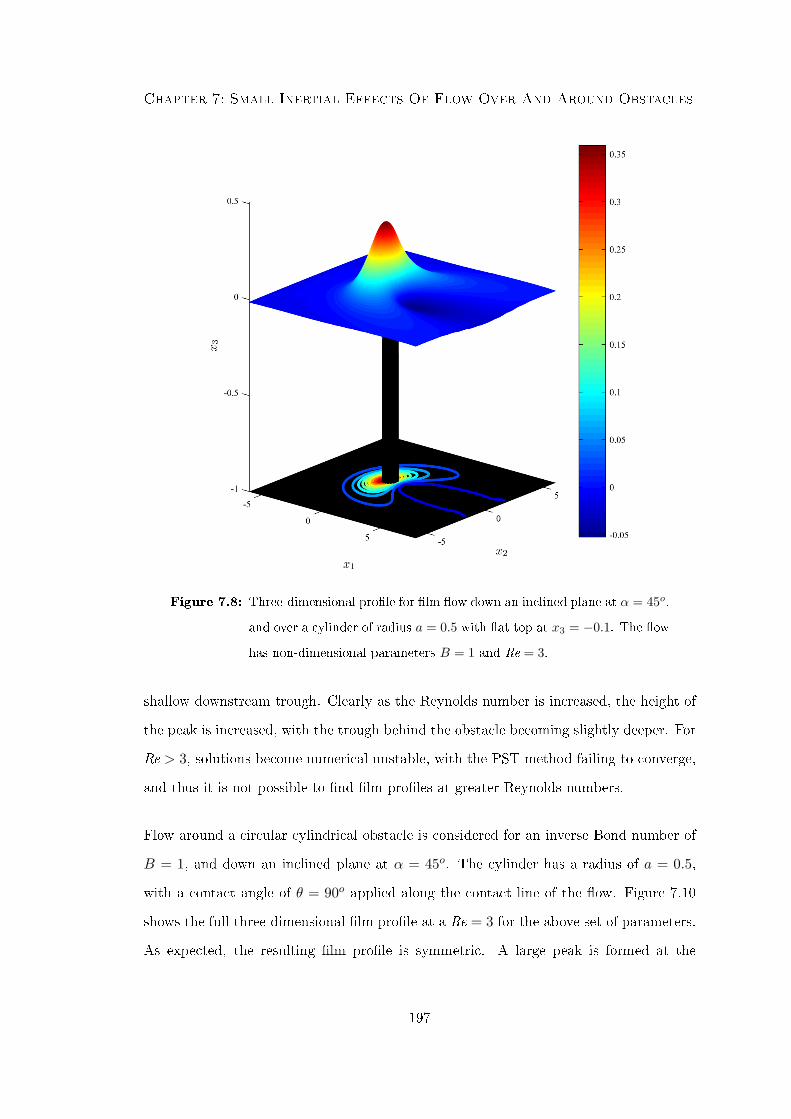
Chapter 7: Small Inertial Effects Of Flow Over And Around Obstacles
Figure 7.8: Three-dimensional prole for lm ow down an inclined plane at α = 45o,
and over a cylinder of radius a = 0.5 with at top at x3 = −0.1. The ow
has non-dimensional parameters B = 1 and Re = 3.
shallow downstream trough. Clearly as the Reynolds number is increased, the height of
the peak is increased, with the trough behind the obstacle becoming slightly deeper. For
Re > 3, solutions become numerical unstable, with the PST method failing to converge,
and thus it is not possible to nd lm proles at greater Reynolds numbers.
Flow around a circular cylindrical obstacle is considered for an inverse Bond number of
B = 1, and down an inclined plane at α = 45o. The cylinder has a radius of a = 0.5,
with a contact angle of θ = 90o applied along the contact line of the ow. Figure 7.10
shows the full three-dimensional lm prole at a Re = 3 for the above set of parameters.
As expected, the resulting lm prole is symmetric. A large peak is formed at the
197
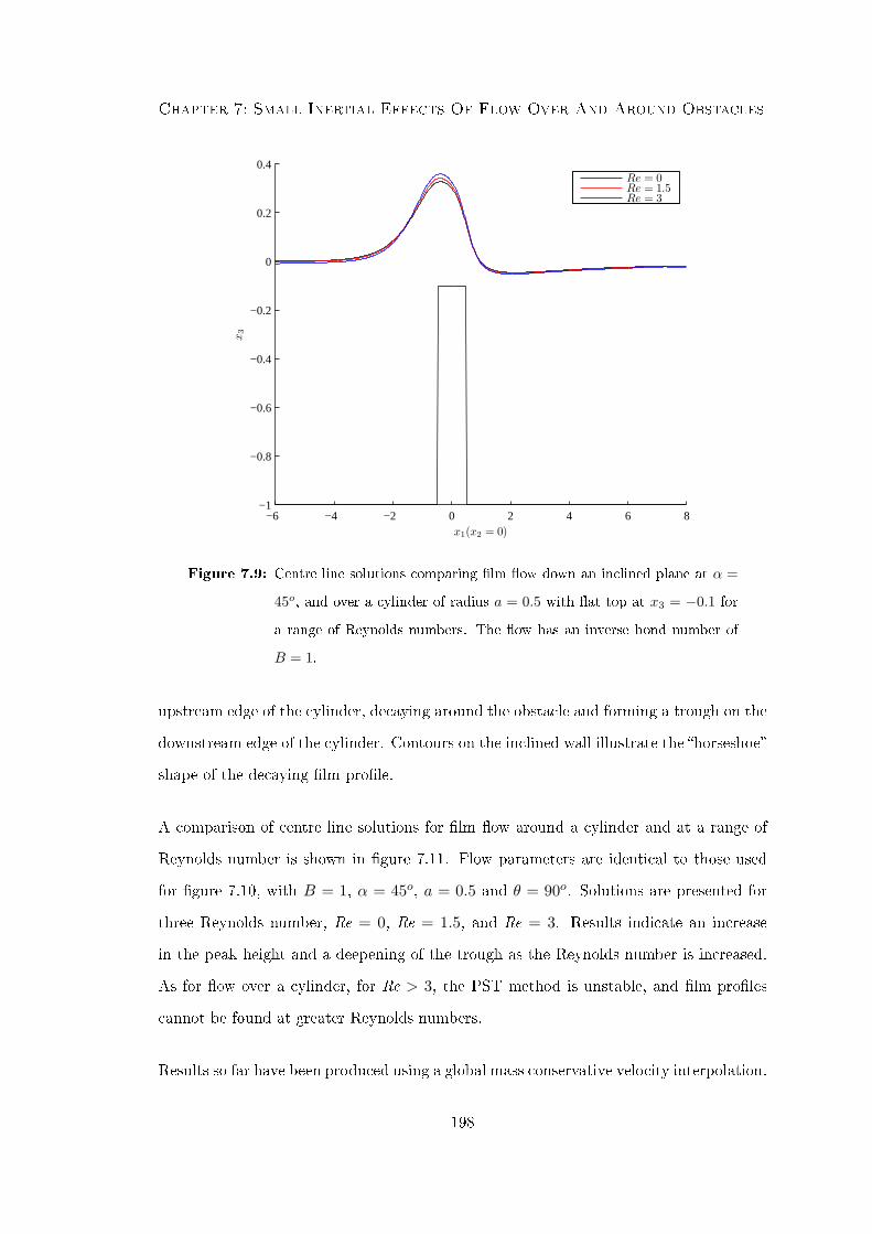
Chapter 7: Small Inertial Effects Of Flow Over And Around Obstacles
−6 −4 −2 0 2 4 6 8−1
−0.8
−0.6
−0.4
−0.2
0
0.2
0.4
x1(x2 = 0)
x3
Re = 0Re = 1.5Re = 3
Figure 7.9: Centre line solutions comparing lm ow down an inclined plane at α =
45o, and over a cylinder of radius a = 0.5 with at top at x3 = −0.1 for
a range of Reynolds numbers. The ow has an inverse bond number of
B = 1.
upstream edge of the cylinder, decaying around the obstacle and forming a trough on the
downstream edge of the cylinder. Contours on the inclined wall illustrate the horseshoe
shape of the decaying lm prole.
A comparison of centre line solutions for lm ow around a cylinder and at a range of
Reynolds number is shown in gure 7.11. Flow parameters are identical to those used
for gure 7.10, with B = 1, α = 45o, a = 0.5 and θ = 90o. Solutions are presented for
three Reynolds number, Re = 0, Re = 1.5, and Re = 3. Results indicate an increase
in the peak height and a deepening of the trough as the Reynolds number is increased.
As for ow over a cylinder, for Re > 3, the PST method is unstable, and lm proles
cannot be found at greater Reynolds numbers.
Results so far have been produced using a global mass conservative velocity interpolation.
198

Chapter 7: Small Inertial Effects Of Flow Over And Around Obstacles
Figure 7.10: Three-dimensional prole for lm ow down an inclined plane at α =
45o, and around a cylinder of radius a = 0.5 with contact angle θ = 90o.
The ow has non-dimensional parameters B = 1 and Re = 3.
As for the case of a lid driven cavity in § 7.2, reductions in both the CPU time and RAM
requirements necessary for the global analysis may be found by implementing a local
interpolation with a suitable number of points. A comparison between the global and
local schemes is considered for ow with an inverse Bond number B = 1, and down
a plane inclined at α = 45o with an attached circular cylinder of radius a = 0.5. For
the ow over analysis, the cylinder is truncated at x3 = −0.1, and for the ow around
analysis a contact angle constraint of θ = 90o implemented. All results are found at a
Reynolds number of Re = 3.
When implementing a local interpolation, less computational resources are required when
199
Chapter 7: Small Inertial Effects Of Flow Over And Around Obstacles
−6 −4 −2 0 2 4 6 8−1
−0.5
0
0.5
x1(x2 = 0)
x3
Re = 0Re = 1.5Re = 3
Figure 7.11: Centre line solutions comparing lm ow down an inclined plane at
α = 45o, around a cylinder of radius a = 0.5 with contact angle θ = 90o
for a range of Reynolds numbers. The ow has an inverse bond number
of B = 1.
fewer local points are chosen. However, when insucient points are used in the local
interpolation, several problems may be experienced with the numerical schemes. If the
number of local points is reduced too severely, then the rate of convergence of the free
surface prole is found to reduce, resulting in signicantly more iterations and the pos-
sibility of longer overall run-times. Alternatively, the PST method can fail completely,
with no ow solution obtained. Therefore, care needs to be taken in choosing an opti-
mum number of local interpolation points, and simulations using both 45 and 51 points
have been considered throughout the following analysis.
Table 7.3 lists the computational performance of global and local schemes (using 45
and 51 points) for both ow over and ow around a circular cylinder. Solutions are
iterated from an undisturbed free surface, with a Stokes ow velocity prole assumed.
200
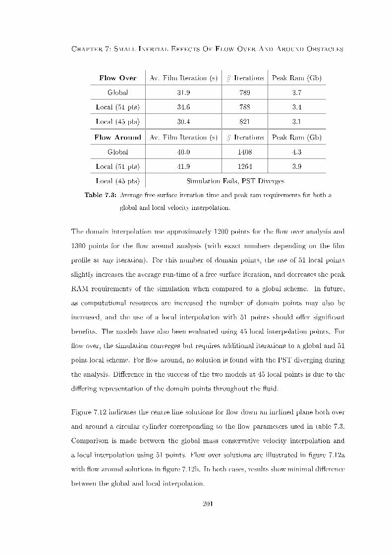
Chapter 7: Small Inertial Effects Of Flow Over And Around Obstacles
Flow Over Av. Film Iteration (s) # Iterations Peak Ram (Gb)
Global 31.9 789 3.7
Local (51 pts) 34.6 788 3.4
Local (45 pts) 30.4 821 3.1
Flow Around Av. Film Iteration (s) # Iterations Peak Ram (Gb)
Global 40.0 1408 4.3
Local (51 pts) 41.9 1264 3.9
Local (45 pts) Simulation Fails, PST Diverges
Table 7.3: Average free surface iteration time and peak ram requirements for both a
global and local velocity interpolation.
The domain interpolation use approximately 1200 points for the ow over analysis and
1300 points for the ow around analysis (with exact numbers depending on the lm
prole at any iteration). For this number of domain points, the use of 51 local points
slightly increases the average run-time of a free surface iteration, and decreases the peak
RAM requirements of the simulation when compared to a global scheme. In future,
as computational resources are increased the number of domain points may also be
increased, and the use of a local interpolation with 51 points should oer signicant
benets. The models have also been evaluated using 45 local interpolation points. For
ow over, the simulation converges but requires additional iterations to a global and 51
point local scheme. For ow around, no solution is found with the PST diverging during
the analysis. Dierence in the success of the two models at 45 local points is due to the
diering representation of the domain points throughout the uid.
Figure 7.12 indicates the centre line solutions for ow down an inclined plane both over
and around a circular cylinder corresponding to the ow parameters used in table 7.3.
Comparison is made between the global mass conservative velocity interpolation and
a local interpolation using 51 points. Flow over solutions are illustrated in gure 7.12a
with ow around solutions in gure 7.12b. In both cases, results show minimal dierence
between the global and local interpolation.
201
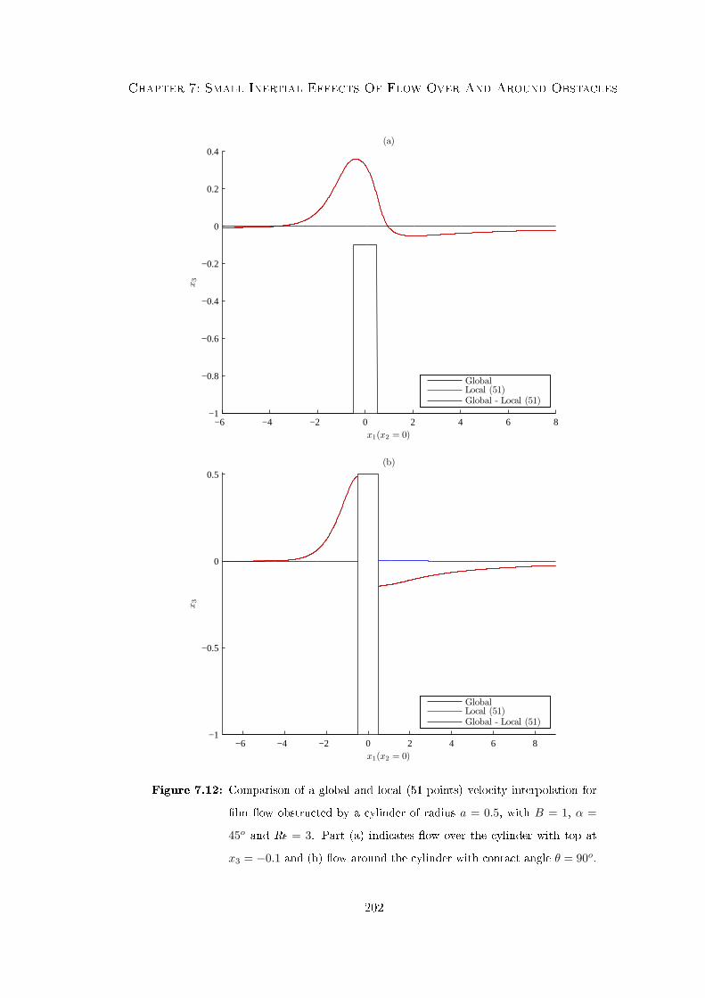
Chapter 7: Small Inertial Effects Of Flow Over And Around Obstacles
−6 −4 −2 0 2 4 6 8−1
−0.8
−0.6
−0.4
−0.2
0
0.2
0.4(a)
x1(x2 = 0)
x3
GlobalLocal (51)Global - Local (51)
−6 −4 −2 0 2 4 6 8−1
−0.5
0
0.5(b)
x1(x2 = 0)
x3
GlobalLocal (51)Global - Local (51)
Figure 7.12: Comparison of a global and local (51 points) velocity interpolation for
lm ow obstructed by a cylinder of radius a = 0.5, with B = 1, α =
45o and Re = 3. Part (a) indicates ow over the cylinder with top at
x3 = −0.1 and (b) ow around the cylinder with contact angle θ = 90o.
202

Chapter 8
Summary And Conclusions
Oil lms are used in aero-engine bearing chambers to cool and transport heat away
from bearings and walls within the oil system. If there is insucient thickness of oil
on the chamber wall, then oil degradation, coking and potentially oil res can occur.
Prediction of lm behaviour is impaired as bearing chambers include complex geometries
such as obstacles that can signicantly aect the local behaviour of the oil lm. The
bearing chamber is a hostile environment for experimental analysis and measurement
of the oil lms interaction with obstructions is dicult. This thesis has considered the
numerical modelling of the interaction of thin lms with obstacles. Methods and results
are provided for single or multiple obstacles which may or may not penetrate the free
surface.
Numerical solutions for three-dimensional Stokes ow down an inclined plane over and
around multiple obstacles have been developed and solutions found by the boundary
element method (BEM). Initially chapter 4 considers ow proles using the small free
surface deection by Blyth and Pozrikidis [31]. A global radial basis function (RBF) is
used throughout to better evaluate the reduced form of the free surface curvature and
outward unit normal. Comparisons are made to the nite dierence approximations
(FDA) used by [31], with results indicating a reduction in mesh dependency for the
RBF approach. For ow over an obstacle, the lm prole is governed by three parame-
ters; inverse Bond number, plane inclination angle, and hemisphere radius. A parameter
203

Chapter 8: Summary And Conclusions
analysis for each of these quantities is also produced using the small free surface deec-
tion assumption. Flow proles over asymptotically small obstacles, such as considered
by Pozrikidis and Thoroddsen [29], have been reproduced and shown to give excellent
agreement with simulations incorporating the full obstacle.
Chapter 4 also extends the small free surface deection assumption by Blyth and Pozrikidis
[31] by using a global RBF interpolation to accurately determine free surface quantities
such as curvature and unit normal for larger surface deections. Comparisons with the
small free surface deection assumption indicate consistency of results for small distur-
bances generated by small hemispheres (a ∼ 20% of lm height). For larger deformations
generated by larger obstacles, solutions using the small deection assumption become
inconsistent with the full analysis. This illustrates the need for removing this restriction
for more general, large obstructions. Streamlines and a parameter analysis for variations
in inverse Bond number and plane inclination are also conducted using this full analysis.
For large hemispheres fully contained within the uid, it is found that the Stokes ow
can support obstacles larger than the undisturbed free surface. The maximum size of
hemisphere is strongly dependent on the inclination of the plane.
The single obstacle analysis is extended to a more general formulation for ow over
arbitrary multiple obstacles in chapter 5. Flows over two, large hemispheres have been
analyzed, with variations in the obstacle locations considered. The eects of separating
the obstacles in-line with the ow has been illustrated, and ow proles shown to return
to those associated with a single obstacle in the case of large separations. In addition
obstacles spaced perpendicular to the incoming ow have been modelled. In this case,
when the obstacles are located close to one another, the ow reacts to the obstacle
as if there is one large obstruction to the ow. A signicantly larger peak is formed,
spanning both obstacles when compared to the cases of moderate and large separations.
Finally two hemispheres spaced diagonally to each other are considered, situating the
downstream hemisphere in the decaying peak of the upstream obstacle, illustrating a
non-symmetric solution. For obstacles aligned in the direction of the ow, a parameter
204
Chapter 8: Summary And Conclusions
study was conducted to investigate the eects of varying the inverse Bond number, plane
inclination angle and hemisphere radius. Flow over two hemispheres that approach the
lm surface have also been modelled, and the eects of placing the downstream obstacle
in the wake of the upstream hemisphere considered. The wake from the upstream obstacle
on both a shallow and a steep plane is shown to reduce the minimum gap between
the free surface and obstacle when compared to a sole obstruction. Finally, ows over
three hemispheres were modelled, with solutions obtained for two obstacle congurations
based on a triangular array. Restrictions on obtaining ow over more obstacles is due to
computational resources.
Chapter 6 extends the formulation further to consider ow around single and multiple
circular cylinders. The incorporation of a contact angle condition within the RBF was
required. For ow around a single cylinder streamline plots are produced along with a
parameter study. For ow around obstacles, there are four governing parameters; inverse
Bond number, plane inclination angle, cylinder radius and contact angle. A comparison
of ow over and around a truncated cylinder indicates the possibility of dual solutions and
indicates the steady state ow prole in this case is dependent on the initial conditions
prescribed and not uniquely by the parameters of the ow eld. Finally, the possibility of
multiple solutions occurring for variations in the underlying ow parameters is conrmed,
with results characterized by the maximum lm height. It is shown that for a suciently
large contact angle, results can be forced around a truncated cylinder for a chosen set of
ow parameters, resulting in dual solutions.
Flows around multiple circular cylinders are also considered in chapter 6. Flow around
two circular cylinders, with various obstacle locations were analyzed. As for ow over
multiple hemispheres, the eects of separating the obstacles in line with the ow have
been illustrated, and ow proles shown to return to those associated with a single obsta-
cle in the case of large separations. For obstacles spaced perpendicular to the incoming
ow and in close proximity, the lm prole between the cylinders becomes signicantly
raised when compared to cylinders at greater separation distances. Finally the non-
205

Chapter 8: Summary And Conclusions
symmetric situation of two cylinders spaced diagonally to each other was modelled, with
the downstream cylinder situated in the decaying peak of the upstream obstacle. When
the cylinders were aligned in the direction of the ow, a parameter study was conducted
to investigate the eects of varying the inverse Bond number, plane inclination angle,
cylinder radius and contact angle. Flow solutions around three cylinders were also con-
sidered, with two obstacle congurations based on the triangular array with dierent
symmetrical orientations to the ow direction. Finally, the versatility of the numerical
approach is demonstrated with the analysis of ow over then around two identical cylin-
ders spaced in the direction of the ow. The eect of the wake caused by the upstream
cylinder was also considered, and shown to allow the contact angle at the downstream
cylinder to be relaxed. As the obstacles are moved closer, the eects of the wake are
strengthened and the contact angle condition can be lowered further.
The above formulations utilize a Stokes ow approximation for the analysis of free surface
lm ows over and around obstacles. The eects of inertia in these ow problems may be
signicant, particularly for dry-out, and the incorporation of the convective term of the
Navier-Stokes equations was considered in chapter 7. However, the lms ows have awk-
ward geometries which require very ecient numerical algorithms to eectively include
the convective term into the integral formulation used for the earlier analysis. Devel-
opment of these ecient numerical algorithms was rst conducted for the common test
problem of ow in a three-dimensional lid driven cavity. This thesis evaluates a formu-
lation for low Reynolds number ows using the BEM to solve the homogeneous solution,
whilst formulating a particular solution using a RBF interpolation. Unlike conventional
formulations such as the particular integral technique (PIT), which linearize the convec-
tive term and solves for domain velocities and unknown boundary tractions together, a
method which solves the particular and homogeneous components separately, called the
particular solution technique (PST) has been implemented. In addition, a local mass
conservative interpolation for the velocity eld has been introduced to further reduce the
necessary computational resources. This local interpolation is an approximation to the
206

Chapter 8: Summary And Conclusions
global analysis, with the accuracy of this method also considered. Solutions for Re = 0,
Re = 100 and Re = 200 are produced by this PST approach using a fraction of the
computational resources that would be required by the conventional PIT.
Chapter 7 uses the optimized numerical scheme developed for the lid-driven cavity test
case and modest computational resources to evaluate low Reynolds number ows over
and around cylindrical obstacles. Solutions are produced using both a global and local
mass conservative interpolation for the velocity eld. Results are obtained for Reynolds
number up to Re = 3, beyond which diculties with convergence of the numerical
schemes was found. However, at Re = 3, changes in the lm prole were observed, with
the lm peak increasing, just before the obstacle, and the trough decreasing behind the
obstruction.
8.1 Future Work
The following possible areas of future work are of particular interest:
• The need remains for extended numerical analysis of ow over and around ob-
stacles, and stems from oil lm ows within bearing chambers, and the complex
support structures which exist. Bearing chambers also include sump regions, and
numerical analysis of ow over three-dimensional trenches and dips would be of
interest.
• In a bearing chamber, the oil lm is driven by surface shear forces as well as gravity.
The eects of including surface shear from the air ow could be considered.
• The eects of perturbations to the free surface prole could be analyzed. This
would be of particular relevance to the multiple solution analysis, determining
which of the two possible solutions (over or around) is most prevalent when sub-
jected to perturbations to the incoming ow.
207

Chapter 8: Summary And Conclusions
• The oil lm within the bearing chamber is used to cool the chamber wall. The
eects of heat transfer from the wall to the thin oil lm could also be considered.
• The analysis could be extended to consider the curvature of a realistic bearing
chamber geometry, instead of a localized ow down an inclined plane.
• In chapter 7 the method outlined for incorporating the inertia eects is convergent
for low Reynolds number. Further development and modication to the numerical
schemes implemented, and increased computational resources may allow conver-
gence for higher Reynolds number.
208

Appendix A
Lorentz-Blake Greens Functions
The Lorentz-Blake Greens functions for ow bounded by an innite plane at x3 = w
are reproduced for our co-ordinate system from Blyth and Pozrikidis [31] and shown
below. The eld point is given by x = (x1, x2, x3) and the singularity point by x0 =
(x01 , x02 , x03).
A.1 Lorentz-Blake Velocity Greens Function
The Lorentz-Blake Velocity Greens function, G∗ij(x,x0) is given by,
G∗ij(x,x0) = GSTij (x)−GSTij (X) + 2h20G
Dij (X)− 2h0G
SDij (X), (A.1.1)
where GSTij is the free-space velocity Greens function or Stokeslet, and
GSTij (x) =δij|x| +
xixj|x|3 , (A.1.2)
GDij (x) = ±(δij|x|3 − 3
xixj|x|5
), (A.1.3)
GSDij (x) = x3GDij (x)± δj3xi − δi3xj
|x|3 , (A.1.4)
where a minus corresponds to j = 3 and a plus for j = 1, 2. Also,
h0 = x03 − w, (A.1.5)
x = x− x0, (A.1.6)
X = x− xIM0 , (A.1.7)
209

Appendix A: Lorentz-Blake Greens Functions
xIM0 = (x01 , x02 , 2w − x03). (A.1.8)
A.2 Lorentz-Blake Pressure Greens Function
The Lorentz-Blake Pressure Greens function, P ∗i (x,x0) is given by,
P ∗i (x,x0) = −2[Xi
|X|3 +Yi|Y|3 2Yi
(− 1|Y|3 + 3
Y 23
|Y|5)
2h(− δi3|Y|3 + 3
Y3Yi|Y|5
)], (A.2.1)
where
h = x3 − w, (A.2.2)
X = x0 − x, (A.2.3)
Y = x0 − xIM , (A.2.4)
xIM = (x1, x2, 2w − x3). (A.2.5)
A.3 Lorentz-Blake Stress Greens Function
The Lorentz-Blake Stress Greens function, T ∗ijk(x,x0) is given by,
T ∗ijk(x,x0) = TSTijk (x)− TSTijk (X) + 2h20T
Dijk(X)− 2h0T
SDijk (X), (A.3.1)
where TSTijk is the free-space stress Greens function, and
TSTijk (x) = 6xixjxk|x|5 , (A.3.2)
TDijk(x) = ±6(−δikxj + δijxk + δkjxi
|x|5 + 5xixjxk|x|7
), (A.3.3)
TSDijk (x) = x3TDijk(x)± 6
(δikxjx3 − δj3xixk
|x|5), (A.3.4)
where a minus corresponds to j = 3 and a plus for j = 1, 2. Also h0, x, X, xIM0 are
dened by (A.1.5) - (A.1.8) respectively.
210

Appendix B
Integrating Dirac's Delta Function
B.1 Integrating Over A Hemisphere
It is known from the standard properties of Dirac's delta function that its integral over a
domain that contains the singularity (see Figure B.1) will result in 1, whilst its integral
over a domain that omits the singularity will result in 0.
The scenario when the point x0 lies directly upon the bounding smooth surface D of the
arbitrary control volume Vc is considered. First, however we note how the delta function
has a radial argument and that its value is zero everywhere except at the singularity,
where it is innite. Consider two spheres, drawn with radius a and b respectively and
Figure B.1: Two illustrations indicating a control volume and singularity, (a) inside
the control volume and (b) outside the control volume.
211

Appendix B: Integrating Dirac's Delta Function
Figure B.2: Illustration indicating the eect of integrating the Dirac delta function
centred on two spheres of dierent radii. The smaller sphere has radius
b and the larger sphere radius a.
with a > b > 0, centred about the singularity point. It is clear that integrating the delta
function over the larger sphere will have the same result as integrating over the smaller
sphere, however small the radius b of this smaller sphere becomes - see Figure B.2.
If the singularity point is now considered to coincide with an arbitrarily shaped smooth
boundary D that describes the control volume Vc, then by drawing a sphere of radius
γ 1 centred on the singularity it is intuitively obvious that the part of the boundary
D within the sphere will tend to a at plane in the limit of γ tending to zero.
Any at plane that intersects a sphere, whilst passing through its centre, will split the
sphere into two equal hemispheres. As contributions to the integral from Dirac's delta
function are only dependent on radius then the orientation of the bisecting plane becomes
insignicant and, ∫SPHERE
δ(x− x0)dV (x) = 2∫
HEMISPHERE
δ(x− x0)dV (x)
= 1.
(B.1.1)
212

Appendix B: Integrating Dirac's Delta Function
Giving the nal result,∫Vc
δ(x− x0)dV (x) =∫
HEMISPHERE
δ(x− x0)dV (x)
=12,
(B.1.2)
as required.
B.2 Integrating Over A Boundary Corner
The case of a singularity placed at a corner of the boundary D is considered, with Dirac's
delta function integrated over the control volume Vc contained by D. As shown in section
B.1, the value of the integral is solely dependent on the shape of the boundary innitely
close to the singularity. Extending this local boundary shape into free-space allows the
calculation of the solid angle of the boundary corner. Drawing a unit sphere around the
singularity will result in an intersection of the extended local boundary shape and the
sphere. This contour will map out a surface area on the sphere, Ω, known as the solid
angle. The solid angle takes values between 0 and 4π, with a value of 2π representing the
hemisphere in the above analysis and 4π representing the entire surface of the sphere.
The units of solid angle is steradians.
From an extension of the previous argument, the integral over a proportion of a spheres
surface (e.g. Ω/4π) is equal to the same proportion multiplied by the integral over the
whole sphere. Thus the integral over a control volume bounded by D , which has the
singularity located at a boundary corner with solid angle Ω, has value∫Vc
δ(x− x0)dV (x) =Ω4π
∫SPHERE
δ(x− x0)dV (x)
=Ω4π.
(B.2.1)
213
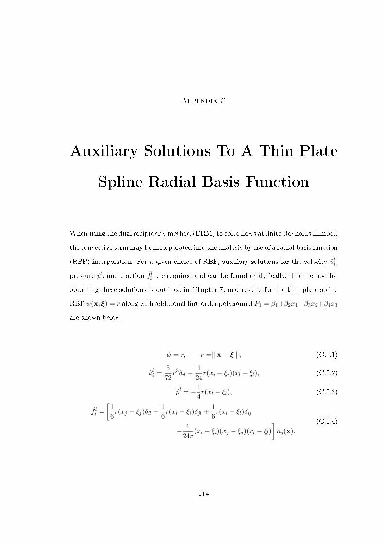
Appendix C
Auxiliary Solutions To A Thin Plate
Spline Radial Basis Function
When using the dual reciprocity method (DRM) to solve ows at nite Reynolds number,
the convective term may be incorporated into the analysis by use of a radial basis function
(RBF) interpolation. For a given choice of RBF, auxiliary solutions for the velocity uli,
pressure pl, and traction f li are required and can be found analytically. The method for
obtaining these solutions is outlined in Chapter 7, and results for the thin plate spline
RBF ψ(x, ξ) = r along with additional rst order polynomial P1 = β1+β2x1+β3x2+β4x3
are shown below.
ψ = r, r =‖ x− ξ ‖, (C.0.1)
uli =572r3δil −
124r(xi − ξi)(xl − ξl), (C.0.2)
pl = −14r(xl − ξl), (C.0.3)
f li =[
16r(xj − ξj)δil +
16r(xi − ξi)δjl +
16r(xl − ξl)δij
− 124r
(xi − ξi)(xj − ξj)(xl − ξl)]nj(x).
(C.0.4)
214
Appendix C: Auxiliary Solutions To A Thin Plate Spline Radial Basis
Function
ψ = x1, (C.0.5)
uli =110(x3
1 + x22x1 + x2
3x1
)δil
− 1280
(4x3
1 [5δ1iδ1l + δ2iδ2l + δ3iδ3l]
+ 4x32 [δ1iδ2l + δ2iδ1l] + 4x2
3 [δ1iδ3l + δ3iδ1l]
+ 12x21x2 [δ1iδ2l + δ2iδ1l] + 12x2
1x3 [δ1iδ3l + δ3iδ1l]
+ 4x22x1 [3δ2iδ2l + 3δ1iδ1l + δ3iδ3l] + 4x2
3x1 [3δ3iδ3l + 3δ1iδ1l + δ2iδ2l]
+ 4x22x3 [δ1iδ3l + δ3iδ1l] + 4x2
3x2 [δ1iδ2l + δ2iδ1l]
+8x1x2x3 [δ3iδ2l + δ2iδ3l]) ,
(C.0.6)
pl = − 110[3x2
1δ1l + x22δ1l + x2
3δ1l + 2x2x1δ2l + 2x3x1δ3l
], (C.0.7)
f li =[
110(3x2
1δ1l + x22δ1l + x2
3δ1l + 2x2x1δ2l + 2x3x1δ3l
)δij
+110(3x2
1δ1j + x22δ1j + x2
3δ1j + 2x2x1δ2j + 2x3x1δ3j
)δil
+110(3x2
1δ1i + x22δ1i + x2
3δ1i + 2x2x1δ2i + 2x3x1δ3i
)δjl
− 12140
x21 [5δ1iδ1jδ1l + δ2iδ1jδ2l + δ3iδ1jδ3l
+δ1iδ2jδ2l + δ2iδ2jδ1l + δ3iδ3jδ1l + δ1iδ3jδ3l]
− 4140
x22 [3δ1iδ2jδ2l + 3δ2iδ2jδ1l + 3δ2iδ1jδ2l
+3δ1iδ1jδ1l + δ1iδ3jδ3l + δ3iδ3jδ1l + δ3iδ1jδ3l]
− 4140
x23 [3δ3iδ1jδ3l + 3δ3iδ3jδ1l + 3δ1iδ3jδ3l
+3δ1iδ1jδ1l + δ2iδ1jδ2l + δ2iδ2jδ1l + δ1iδ2jδ2l]
− 8140
x1x2 [3δ1iδ1jδ2l + 3δ1iδ2jδ1l + 3δ2iδ2jδ2l
+3δ2iδ1jδ1l + δ2iδ3jδ3l + δ3iδ3jδ2l + δ3iδ2jδ3l]
− 8140
x1x3 [3δ1iδ3jδ1l + 3δ1iδ1jδ3l + 3δ3iδ3jδ3l
+3δ3iδ1jδ1l + δ3iδ2jδ2l + δ2iδ3jδ2l + δ2iδ2jδ3l]
− 8140
x2x3 [δ2iδ3jδ1l + δ2iδ1jδ3l + δ3iδ2jδ1l
+δ3iδ1jδ2l + δ1iδ3jδ2l + δ1iδ2jδ3l]]nj(x).
(C.0.8)
215
Appendix C: Auxiliary Solutions To A Thin Plate Spline Radial Basis
Function
ψ = x2, (C.0.9)
uli =110(x3
2 + x21x2 + x2
3x2
)δil
− 1280
(4x3
2 [5δ2iδ2l + δ1iδ1l + δ3iδ3l]
+ 4x31 [δ2iδ1l + δ1iδ2l] + 4x2
3 [δ2iδ3l + δ3iδ2l]
+ 12x22x1 [δ2iδ1l + δ1iδ2l] + 12x2
2x3 [δ2iδ3l + δ3iδ2l]
+ 4x21x2 [3δ1iδ1l + 3δ2iδ2l + δ3iδ3l] + 4x2
3x2 [3δ3iδ3l + 3δ2iδ2l + δ1iδ1l]
+ 4x21x3 [δ2iδ3l + δ3iδ2l] + 4x2
3x1 [δ2iδ1l + δ1iδ2l]
+8x2x1x3 [δ3iδ1l + δ1iδ3l]) ,
(C.0.10)
pl = − 110[3x2
2δ2l + x21δ2l + x2
3δ2l + 2x1x2δ1l + 2x3x2δ3l
], (C.0.11)
f li =[
110(3x2
2δ2l + x21δ2l + x2
3δ2l + 2x1x2δ1l + 2x3x2δ3l
)δij
+110(3x2
2δ2j + x21δ2j + x2
3δ2j + 2x1x2δ1j + 2x3x2δ3j
)δil
+110(3x2
2δ2i + x21δ2i + x2
3δ2i + 2x1x2δ1i + 2x3x2δ3i
)δjl
− 12140
x22 [5δ2iδ2jδ2l + δ1iδ2jδ1l + δ3iδ2jδ3l
+δ2iδ1jδ1l + δ1iδ1jδ2l + δ3iδ3jδ2l + δ2iδ3jδ3l]
− 4140
x21 [3δ2iδ1jδ1l + 3δ1iδ1jδ2l + 3δ1iδ2jδ1l
+3δ2iδ2jδ2l + δ2iδ3jδ3l + δ3iδ3jδ2l + δ3iδ2jδ3l]
− 4140
x23 [3δ3iδ2jδ3l + 3δ3iδ3jδ2l + 3δ2iδ3jδ3l
+3δ2iδ2jδ2l + δ1iδ2jδ1l + δ1iδ1jδ2l + δ2iδ1jδ1l]
− 8140
x2x1 [3δ2iδ2jδ1l + 3δ2iδ1jδ2l + 3δ1iδ1jδ1l
+3δ1iδ2jδ2l + δ1iδ3jδ3l + δ3iδ3jδ1l + δ3iδ1jδ3l]
− 8140
x2x3 [3δ2iδ3jδ2l + 3δ2iδ2jδ3l + 3δ3iδ3jδ3l
+3δ3iδ2jδ2l + δ3iδ1jδ1l + δ1iδ3jδ1l + δ1iδ1jδ3l]
− 8140
x1x3 [δ1iδ3jδ2l + δ1iδ2jδ3l + δ3iδ1jδ2l
+δ3iδ2jδ1l + δ2iδ3jδ1l + δ2iδ1jδ3l]]nj(x).
(C.0.12)
216
Appendix C: Auxiliary Solutions To A Thin Plate Spline Radial Basis
Function
ψ = x3, (C.0.13)
uli =110(x3
3 + x22x3 + x2
1x3
)δil
− 1280
(4x3
3 [5δ3iδ3l + δ2iδ2l + δ1iδ1l]
+ 4x32 [δ3iδ2l + δ2iδ3l] + 4x2
1 [δ3iδ1l + δ1iδ3l]
+ 12x23x2 [δ3iδ2l + δ2iδ3l] + 12x2
3x1 [δ3iδ1l + δ1iδ3l]
+ 4x22x3 [3δ2iδ2l + 3δ3iδ3l + δ1iδ1l] + 4x2
1x3 [3δ1iδ1l + 3δ3iδ3l + δ2iδ2l]
+ 4x22x1 [δ3iδ1l + δ1iδ3l] + 4x2
1x2 [δ3iδ2l + δ2iδ3l]
+8x3x2x1 [δ1iδ2l + δ2iδ1l]) ,
(C.0.14)
pl = − 110[3x2
3δ3l + x22δ3l + x2
1δ3l + 2x2x3δ2l + 2x1x3δ1l
], (C.0.15)
f li =[
110(3x2
3δ3l + x22δ3l + x2
1δ3l + 2x2x3δ2l + 2x1x3δ1l
)δij
+110(3x2
3δ3j + x22δ3j + x2
1δ3j + 2x2x3δ2j + 2x1x3δ1j
)δil
+110(3x2
3δ3i + x22δ3i + x2
1δ3i + 2x2x3δ2i + 2x1x3δ1i
)δjl
− 12140
x23 [5δ3iδ3jδ3l + δ2iδ3jδ2l + δ1iδ3jδ1l
+δ3iδ2jδ2l + δ2iδ2jδ3l + δ1iδ1jδ3l + δ3iδ1jδ1l]
− 4140
x22 [3δ3iδ2jδ2l + 3δ2iδ2jδ3l + 3δ2iδ3jδ2l
+3δ3iδ3jδ3l + δ3iδ1jδ1l + δ1iδ1jδ3l + δ1iδ3jδ1l]
− 4140
x21 [3δ1iδ3jδ1l + 3δ1iδ1jδ3l + 3δ3iδ1jδ1l
+3δ3iδ3jδ3l + δ2iδ3jδ2l + δ2iδ2jδ3l + δ3iδ2jδ2l]
− 8140
x3x2 [3δ3iδ3jδ2l + 3δ3iδ2jδ3l + 3δ2iδ2jδ2l
+3δ2iδ3jδ3l + δ2iδ1jδ1l + δ1iδ1jδ2l + δ1iδ2jδ1l]
− 8140
x3x1 [3δ3iδ1jδ3l + 3δ3iδ3jδ1l + 3δ1iδ1jδ1l
+3δ1iδ3jδ3l + δ1iδ2jδ2l + δ2iδ1jδ2l + δ2iδ2jδ1l]
− 8140
x2x1 [δ2iδ1jδ3l + δ2iδ3jδ1l + δ1iδ2jδ3l
+δ1iδ3jδ2l + δ3iδ1jδ2l + δ3iδ2jδ1l]]nj(x).
(C.0.16)
217

Appendix C: Auxiliary Solutions To A Thin Plate Spline Radial Basis
Function
ψ = 1, r =‖ x ‖, (C.0.17)
uli =215r2δil −
115xixl, (C.0.18)
pl = −13xl, (C.0.19)
f li =[
15xiδjl +
15xjδil +
15xlδij
]nj(x). (C.0.20)
218

References
[1] C. Eastwick, K. Simmons, K. Huebner, C. Young, B. Azzopardi, and R. Morrison.
Film ow around bearing chamber support structures. Proceedings of ASME Turbo
Exp 2005: Power for Land, Sea and Air, Nevada, June 6-9, 2005.
[2] S. Wittig, A. Glahn, and J. Himmelsbach. Inuence of high rotational speeds on
heat transfer and oil lm thickness in aero-engine bearing chambers. Journal of
Engineering for Gas Turbines and Power, 116(2):395401, 1994.
[3] A. Glahn and S. Wittig. Two-phase air/oil ow in aero engine bearing chambers:
Characterization of oil lm ows. Journal of Engineering for Gas Turbines and
Power, 118(3):578583, 1996.
[4] M. Farrall, S. Hibberd, K. Simmons, and D. Giddings. Prediction of air/oil exit
ows in a commercial aero-engine bearing chamber. Proceedings of the Institution
of Mechanical Engineers, Part G: Journal of Aerospace Engineering, 220(3):197
202, 2006.
[5] M. Farrall, K. Simmons, S. Hibberd, and P. Gorse. A numerical model for oil
lm ow in an aeroengine bearing chamber and comparison to experimental data.
Journal of Engineering for Gas Turbines and Power, 128(1):111117, 2006.
[6] M. Farrall, S. Hibberd, and K. Simmons. The eect of initial injection conditions
on the oil droplet motion in a simplied bearing chamber. Journal of Engineering
for Gas Turbines and Power, 130(1):0125017, 2008.
219

References
[7] O.A. Kabov. Heat transfer from a small heater to a falling liquid lm. Heat Transfer
Research, 27(1):221226, 1996.
[8] O.A. Kabov and I.V. Marchuk. Infrared study of the liquid lm owing on surface
with nonuniform heat ux distribution. Heat Transfer Research, 29(6):544562,
1998.
[9] O.A. Kabov, B. Scheid, I.A. Sharina, and J.C. Legros. Heat transfer and rivulet
structures formation in a falling thin liquid lm locally heated. International Journal
of Thermal Sciences, 41(7):664672, 2002.
[10] S. Shetty and R.L. Cerro. Spreading of a liquid point source over a complex surface.
Industrial & Engineering Chemistry Research, 37(2):626635, 1998.
[11] K. Argyriadi, M. Vlachogiannis, and V. Bontozoglou. Experimental study of inclined
lm ow along periodic corrugations: The eect of wall steepness. Physics of Fluids,
18(1):012102, 2006.
[12] L.E. Stillwagon and R.G. Larson. Leveling of thin lms over uneven substrates
during spin coating. Physics of Fluids A, 2(11), 1990.
[13] L.M. Peurrung and D.B. Graves. Film thickness proles over topography in spin
coating. Journal of The Electrochemical Society, 138(7):21152124, 1991.
[14] M.M.J. Decré and J.-C. Baret. Gravity-driven ows of viscous liquids over two-
dimensional topographies. Journal of Fluid Mechanics, 487:147166, 2003.
[15] B.S. Shiralkar and R.T. Lahey. The eect of obstacles on a liquid lm. Journal of
Heat Transfer, pages 528533, 1973.
[16] J.M. Skotheim, U.W.E. Thiele, and B. Scheid. On the instability of a falling lm
due to localized heating. Journal of Fluid Mechanics, 475:119, 2003.
[17] B. Scheid, A. Oron, P. Colinet, U. Thiele, and J.C. Legros. Nonlinear evolution of
nonuniformly heated falling liquid lms. Physics of Fluids, 14(12):41304151, 2002.
220
References
[18] C.Y. Wang. Liquid lm owing slowly down a wavy incline. AIChE Journal, 27(2):
207212, 1981.
[19] C. Pozrikidis. The ow of a liquid lm along a periodic wall. Journal of Fluid
Mechanics, 188:275300, 1988.
[20] C. Pozrikidis. Eect of surfactants on lm ow down a periodic wall. Journal of
Fluid Mechanics, 496:105127, 2003.
[21] N.A. Malamataris and V. Bontozoglou. Computer aided analysis of viscous lm
ow along an inclined wavy wall. Journal of Computational Physics, 154(2):372
392, 1999.
[22] S. Kalliadasis, C. Bielarz, and G.M. Homsy. Steady free-surface thin lm ows over
topography. Physics of Fluids, 12(8):18891898, 2000.
[23] A. Mazouchi and G.M. Homsy. Free surface stokes ow over topography. Physics
of Fluids, 13(10):27512761, 2001.
[24] E.B. Hansen. Free surface stokes ow over an obstacle. In Boundary Elements VIII,
Tokyo, Japan, 1986.
[25] E.B. Hansen. Stokes ow of a uid layer over an obstacle on a tilted plane. Mathe-
matical and Computer Modelling, 15:195193, 1991.
[26] N.H. Shuaib. Numerical simulation of thin lm ow including surface shear and
gravitational eects. PhD thesis, University of Nottingham, 2004.
[27] M. Hayes, G. O'Brien, and J.H. Lammers. Green's function for steady ow over a
small two-dimensional topography. Physics of Fluids, 12(11):28452858, 2000.
[28] P.H. Gaskell, P.K. Jimack, M. Sellier, H.M. Thompson, and M.C.T. Wilson.
Gravity-driven ow of continuous thin liquid lms on non-porous substrates with
topography. Journal of Fluid Mechanics, 509(1):253280, 2004.
221

References
[29] C. Pozrikidis and S.T. Thoroddsen. The deformation of a liquid lm owing down
an inclined plane wall over a small particle arrested on the wall. Physics of Fluids
A, 3(11):25462558, 1991.
[30] Y.C. Lee, H.M. Thompson, and P.H. Gaskell. An ecient adaptive multigrid al-
gorithm for predicting thin lm ow on surfaces containing localised topographic
features. Computers & Fluids, 36:838855, 2007.
[31] M.G. Blyth and C. Pozrikidis. Film ow down an inclined plane over a three-
dimensional obstacle. Physics of Fluids, 18(5):05210414, 2006.
[32] M. Sellier. The ow of a thin liquid lm past a cylinder. In COMSOL Users
Conference 2006, pages 151154, Frankfurt, 2006.
[33] M. Sellier, Y.C. Lee, H.M. Thompson, and P.H. Gaskell. Thin lm ow on surfaces
containing arbitrary occlusions. Computers & Fluids, 38(1):171182, 2009.
[34] C. Pozrikidis. A Practical Guide to Boundary Element Methods with the Software
Library BEMLIB. Chapman & Hall/CRC, Florida, 2002.
[35] H. Power and L.C. Wrobel. Boundary Integral Methods in Fluid Mechanics. Com-
putational Mechanics Publications, Southampton, 1995.
[36] C. Pozrikidis. Introduction to Theoretical and Computational Fluid Dynamics. Ox-
ford University Press, New York, 1997.
[37] C. Pozrikidis. Boundary integral and singularity methods for linearized viscous ow.
Cambridge University Press, Cambridge, 1992.
[38] D.J. Acheson. Elementary Fluid Mechanics. Oxford University Press, New York,
2003.
[39] H. Ockendon and J.R. Ockendon. Viscous Flow. Cambridge Texts in Applied
Mathematics. Cambridge University Press, New York, 1995.
222
References
[40] R. Franke. Scattered data interpolation: Tests of some method. Mathematics of
Computation, 38(157):181200, 1982.
[41] A. La Rocca, A. Hernandez Rosales, and H. Power. Radial basis function her-
mite collocation approach for the solution of time dependent convection-diusion
problems. Engineering Analysis with Boundary Elements, 29(4):359370, 2005.
[42] A. La Rocca and H. Power. A double boundary collocation hermitian approach for
the solution of steady state convection-diusion problems. Computers & Mathemat-
ics with Applications, 55(9):19501960, 2008.
[43] D. Nardini and C.A. Brebbia. A new approach to free vibration analysis using
boundary elements. Applied Mathematical Modelling, 7(3):157162, 1983.
[44] M.A. Golberg and C.S. Chen. Discrete projection methods for integral equations.
Computational Mechanics Publication, Southampton, 1997.
[45] M.J.D. Powell. The uniform convergence of thin plate spline interpolation in two
dimensions. Numerische Mathematik, 68(1):107128, 1994.
[46] W.R. Madych and S.A. Nelson. Multivariate interpolation and conditionally positive
denite functions. ii. Mathematics of Computation, 54(189):211230, 1990.
[47] R. Schaback. Multivariate interpolation and approximation by translates of a basis
function. In C.K. Chui and L.L. Schumaker, editors, Approximation theory VIII.
World Scientic Publishing Co., Inc., 1995.
[48] M.E. O'Neill. A sphere in contact with a plane wall in a slow linear shear ow.
Chemical Engineering Science, 23(11):12931298, 1968.
[49] G. Krishnasamy, F.J. Rizzo, and Y. Liu. Boundary integral equations for thin
bodies. International Journal for Numerical Methods in Engineering, 37:107121,
1994.
223

References
[50] J.C. Lachat and J.O. Watson. Eective numerical treatment of boundary integra-
tions: A formulation for three-dimensional elastostatics. International Journal for
Numerical Methods in Engineering, 10(5):9911005, 1976.
[51] K.A. Hayami. Projection transformation method for near singular surface bound-
ary element integrals (Lecture Notes in Engineering), volume 73. Springer-Verlag,
Berlin, 1992.
[52] Y.Mi and M.H. Aliabadi. Taylor expansion algorithm for integration of 3d near-
hypersingular integrals. Communications in Numerical Methods in Engineering, 12
(1):51, 1996.
[53] V. Cutanda, P.M. Juhl, and F. Jacobsen. On the modelling of narrow gaps using
standard boundary element method. Journal of the Acoustical Society of America,
109(4):12961303, 2001.
[54] S. Ahmad and P.K. Banerjee. Free vibration analysis by bem using particular
integrals. Journal of Engineering Mechanics, 112(7):682695, 1986.
[55] H. Power and V. Botte. An indirect boundary element method for solving low
reynolds number navier-stokes equations in a three-dimensional cavity. International
Journal for Numerical Methods in Engineering, 41(8):14851505, 1998.
[56] W.F. Florez and H. Power. Drm multidomain mass conservative interpolation ap-
proach for the bem solution of the two-dimensional navier-stokes equations. Com-
puters and Mathematics with Applications, 43(3-5):457472, 2002.
[57] T. Yamada, L.C. Wrobel, and H. Power. On the convergence of the dual reciprocity
boundary element method. Engineering Analysis with Boundary Elements, 13(3):
291298, 1994.
[58] J.-Y. Yang, S.-C. Yang, Y.-N. Chen, and C.-A. Hsu. Implicit weighted eno schemes
for the three-dimensional incompressible navier-stokes equations. Journal of Com-
putational Physics, 146(1):464487, 1998.
224