NUMERICAL SIMULATION OF THE TEMPERATURE HISTORY FOR PLASTIC PARTS IN FUSED FILAMENT FABRICATION (FFF) PROCESS

D. Zeng*, Matthew Rebandt*, Giuseppe Lacaria* Ellen Lee*, Xuming Su*

*Ford Motor Company

Jinglin Zheng†, Xinhai Zhu† †Livermore Software Technology Corporation

Abstract

Fused Filament Fabrication (FFF) is one of the major Additive Manufacturing (AM) processes for polymer materials. In FFF process, repetitive heating and cooling cycles occur when the filament is dispositioned onto a build platform to fabricate a three-dimensional part. The uneven temperature gradients and non-uniform cooling in the part may cause significant amount of warpage. The current practice of making an AM part to match the design intent is largely relied on time consuming trial-and-errors. Numerical simulation is an effective way to predict warpage. Accurate prediction of the thermal history during the FFF process is key for the success of warpage simulation. In this paper, an integrated approach is developed in LS-DYNA to model the FFF process and predict the temperature profile. Different from the traditional approaches, the tool path and FEM mesh are decoupled in this study to enable the flexibility of FEA mesh generation and improve computational efficiency. An innovated micro thermocouple is used to measure the temperature history inside the parts. The evolution of the thermal history is predicted and compared to the measurement data to demonstrate the accuracy and efficiency of the developed simulation model.

Introduction

Additive manufacturing is a rapidly growing technology due to its ability to make parts with complex geometries. In Fused Fabric Filament (FFF) process, a solid polymer filament is melt, extruded through a nozzle, welded onto neighboring materials, solidified during cooling. During the process, non-uniform temperature field is developed due to the repetitive heating and cooling cycles, which may induce significant amount of warping in the parts. Especially, polymers are poor in conducting heat. Significant temperature gradients can exist within the polymer. Thus, it is important to understand the evolution of filament temperature during material deposition and cooling and also how it is affected by the process parameters.

To simulate the temperature evolution and predict warpage for AM processes, analytical and numerical models were developed [1-3]. Costa et al. [2] developed an analytical solution in Matlab to model the transient heat conduction during filament deposition in Fused Deposition Techniques (FDT). The predictions correlated well with the measurements of filament temperature and adhesion. Amado et al. [3] presented a model to describe the warpage development during the crystallization phase of a thermoplastic material in Selective Laser Sintering (SLS) process. A multi-physics approach was applied to connect the thermal, mechanical and phase change physics. However, in most models, the size and complexity of the simulation part as well as the simulated number of layers are limited by the required calculation time, which can take hours and days, depending on the FEA mesh and time steps. Keller and

1230

Solid Freeform Fabrication 2019: Proceedings of the 30th Annual InternationalSolid Freeform Fabrication Symposium – An Additive Manufacturing Conference

Ploshikhin [4] developed a multiscale approach to enable much faster predictions of residual stress and distortion for AM parts. The accuracy of the prediction in this approach is largely depended on the calibration of the so-called inherent strain, which is the mechanical layer equivalent property. To speed up the simulation, most of the approaches for distortion and deformation prediction of additive manufactured parts are based on the layer by layer discretization. In addition, layers are combined to reduce the computational time. Although the simulations can be enabled by these approximations, most influences of the process itself are neglected.

In order to accurately capture the temperature evolution and predict the warpage in FFF process, filaments have to be discretized based on the printing path and modeled in real deposition speed. In the meantime, the calculation time must be reduced radically for practical usage. In this work, an integrated approach is developed to simulate the FFF process for polymer materials in LS-DYNA. Different from the traditional approach, the tool path and FEA mesh are decoupled to enable the flexibility in mesh generation and improve the computational efficiency. The focus of this paper is on the thermal analysis for temperature field prediction. The temperature evolution during the process is predicted and validated through measurement data.

In most literatures, a suitable correlation was presented between simulation and experimental results. Normally, process temperature has been measured through pyrometers or infrared (IR) cameras [5-7]. For example, Seppala and Migler [5] used IR thermography to measure the spatial and temporal temperature profiles under different printing conditions to study the active printing region of the weld zone. The pyrometers and IR cameras can monitor temperature profile on the part surface. However it is challenging to directly measure the temperature evolution inside the plastic parts during the entire process. Especially, since the polymer is poor in conducting of heat, it does not dissipate the heat away as quickly and effectively as desired. Significant temperature gradients can exist within the polymer resulting in strong spatial and temporal variations. Regular thermal couple is too large in size and thermal mass. It is difficult to place a thermocouple in the flow stream without destroying the process. In this paper, a micro thermocouple measured the temperature history and provided reliable data for model validation. The simulation of a dog-bone shape tensile bar printed in FFF process illustrated the model development and validation approaches.

Development of simulation model for FFF process in LS-DYNA

In this study, we integrated some of the latest technologies developed in commercial FEA software LS-DYNA to simulate the FFF printing process. Following are some of the key features adopted and/or newly developed in LS-DYNA:

1) Printing path for material deposition To model the material deposition process, elements are usually progressively activated along the print path [8]. Voxel mesh (as shown in Figure 1(a)) is typically used to discretize the filaments. A voxel mesh is a set of regular brick elements. The mesh size is largely determined by the layer height. Large mesh size will result in zigzags along the part boundary. While tremendous number of elements will be generated when the mesh size is small. In this study, material deposition is realized through the change of state in material model instead of element activation and deactivation modeling. Thus, the element mesh is not dependent on the

1231

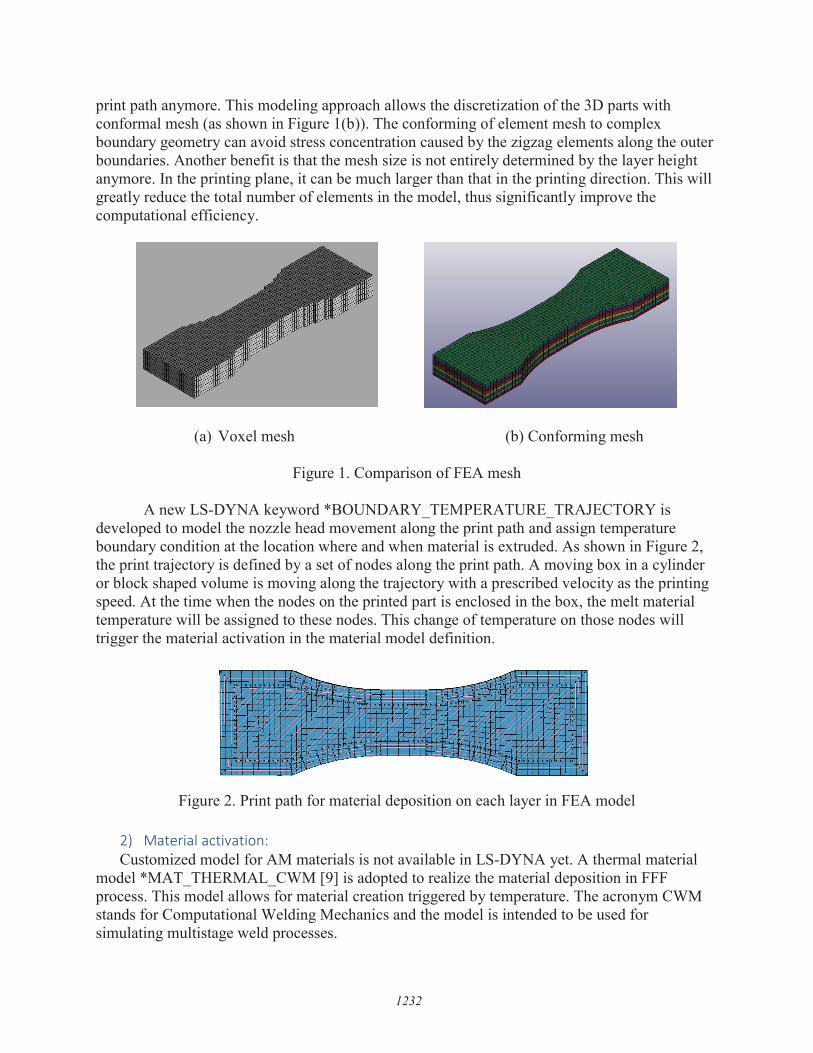
print path anymore. This modeling approach allows the discretization of the 3D parts with conformal mesh (as shown in Figure 1(b)). The conforming of element mesh to complex boundary geometry can avoid stress concentration caused by the zigzag elements along the outer boundaries. Another benefit is that the mesh size is not entirely determined by the layer height anymore. In the printing plane, it can be much larger than that in the printing direction. This will greatly reduce the total number of elements in the model, thus significantly improve the computational efficiency.

(a) Voxel mesh (b) Conforming mesh

Figure 1. Comparison of FEA mesh

A new LS-DYNA keyword *BOUNDARY_TEMPERATURE_TRAJECTORY is developed to model the nozzle head movement along the print path and assign temperature boundary condition at the location where and when material is extruded. As shown in Figure 2, the print trajectory is defined by a set of nodes along the print path. A moving box in a cylinder or block shaped volume is moving along the trajectory with a prescribed velocity as the printing speed. At the time when the nodes on the printed part is enclosed in the box, the melt material temperature will be assigned to these nodes. This change of temperature on those nodes will trigger the material activation in the material model definition.

Figure 2. Print path for material deposition on each layer in FEA model

2) Material activation: Customized model for AM materials is not available in LS-DYNA yet. A thermal material

model *MAT_THERMAL_CWM [9] is adopted to realize the material deposition in FFF process. This model allows for material creation triggered by temperature. The acronym CWM stands for Computational Welding Mechanics and the model is intended to be used for simulating multistage weld processes.

1232

At the beginning before the material is deposited, the material in the model is defined as a

quiet state for all of the elements. The material in this state sometimes is referred to as ghost material. A relatively large specific heat and small thermal conductivity is assigned to represent the empty space. The value of the thermal conductivity should be small enough to not influence the surroundings but large enough to avoid numerical problems. When the nozzle starts to extrude material, elements at the material deposition location become active As far as the temperature of the elements in ghost state reaches a specified temperature level, the material thermal properties are changed to those of the filament material. This activation temperature is assigned from the new keyword *BOUNDARY_TEMPERATURE_TRAJECTORY introduced above. Temperature dependent thermal properties from literatures [10] will be incorporated into the model.

3) Interface modeling: Contact cards with thermal option are applied to model the heat flow at the interfaces

between the polymer and glass build plate. The TIED_WELD option in the contact card is added to model the interface between two polymer layers. This contact option in LS-DYNA was developed to activate a condition where sliding contact will become tied contact on cool down when the temperature of the segments in contact go above an input specified temperature limit during welding. This card is adopted in this study to simulate the top layer of material before and after deposition on the lower layer.

The thermal contact conductance is the parameter to define the thermal conductivity between

two solids. It is influenced by many factors like contact pressure, Interstitial materials, Surface roughness, waviness and flatness, etc. [11]. Most experimentally determined values of the thermal contact resistance fall between 2 to 200 mW/mm² K [12].

FFF Process Simulation Model Setup and Results With all the keywords defined, the printing process of a tensile bar using Ultimaker 3 printer

is modeled to illustrate the developed modeling approach.

1) Tensile bar printed in FFF process with Ultimaker 3 Extended printer As shown in Figure 3, there are a large number of process parameters need to be defined for a given part geometry, including temperature in chamber, in nozzle and on the build plate, print orientation, print path pattern, part slicing parameters like nozzle diameter, layer height, infill percentage, etc. The bead width and bead gap determine the infill, as in Equation (1).

Infill percentage =

(1)

1233

(a) Print orientation (b) Print path pattern (c) Slicing parameters

Figure 3. Illustration of print parameters in FFF process

As in Figure 4, a one and half inch long dog-bone shape tensile bar with 3.2mm in thickness is printed with Ultimaker 3 Extended printer. This printer can print parts with complex geometries and mixed materials. It is easy to use. An open source program Ultimaker Cura is used to automatically create the process parameters and generate a print path file in gecode format based on the part geometry. The process parameters can also be modified at user’s choice in Ultimaker Cura program.

Figure 4. A tensile bar printed with Ultimaker 3 Extended printer

Acrylonitrile Butadiene Styrene (ABS) filament is considered in this study. A nozzle in diameter of 0.4mm is used. The layer height is also set to be 0.4mm. So there are eight printing layers in total. The first layer is adhered to the glass build plate with glue sticks. The sample is printed with alternative ±45 degree bead direction with respect to the axis of the tensile bar in the printing plane. Figure 5 shows the print path for each layer.

1234

(a) Print path for odd layer (b) Print path for even layer

(b) Figure 5 Illustration of print path at each layer

The process parameters are listed in Table 1. These are key parameters which will be

used for simulation model setup.

Table 1. Summary of process parameters

2) Simulation model setup

The FEA model is built based on the above print parameters in real printing process. The model is discretized with conforming mesh with one layer of glass build plate on the bottom and eight layers of ABS polymer. As shown in Figure 6, the curvatures on the part are nicely captured with the conforming mesh. Thermal contact cards are defined between each layers. The print path is discretized into nodes which make a nodal path as the input for the keyword *BOUNDARY_TEMPERATURE_TRAJECTORY. All of the nodes at the bottom of the glass plates are fixed and assigned an 80oC temperature boundary condition.

Thermal material properties are defined for both glass plate and ABS polymer. For ABS polymer, the material is defined in two states. Below the birth temperature, which is the temperature of material melt, the material of all the elements is in ghost state. A small value (10-

4) is assigned to the thermal conductivity. When the temperature of the material reaches the birth temperature, the material is activated. The filament material properties are defined. Only active material properties are defined for glass plate. Once all the keywords for print path, material and contact interface are defined, an integrated FEA model are used to predict the temperature history for the FFF process.

Extruder temperature 230 0CBuild plate temperature 80 0CLayer infill percentage 100%Bead width 0.3mmBead gap 0.3mmLayer height 0.4mmInfill print speed 25mm/s

1235

Figure 6. Conforming FEM mesh for the tensile bar

3) Simulation results

Only thermal analysis is conducted to predict the part temperature history in this paper. In the future study, thermal mechanical analysis will be developed in combination with the mechanical counterpart *MAT_CWM in LS-DYNA to calculate the residual stress caused by the non-uniform heating and cooling process and predict part warpage.

Figure 7 shows the temperature profile at the time when the material is deposited on the first

layer. Before the material starts to be extruded, initial temperature of 800C is assigned to all the nodes belonging to first layer. The elements in this layer are in ghost state. As shown in Figure 7(a), when the print head starts to extrude material, the extrude temperature of 2300C is assigned to the nodes along the print path. The material is not in ghost state anymore. After the print head passes by, the material will start to cool down due to heat exchange with neighboring material. However, the material will be go back to ghost state anymore. Figure 7(b) shows the temperature profile at the end of the first layer printing. All the material has been activated in this layer.

(a) At the start of material deposition on 1st layer

1236

Nodal discretization of the print path on odd layer ........_

} Printed polymer layers

Temperature, middle

2.300e+02

2.150e+02

2.000e+02

1.850e+02

1.700e+02

1.550e+02

1.400e+02

1.250e+02

1.100e+02

9.500e+01

8.000e+01

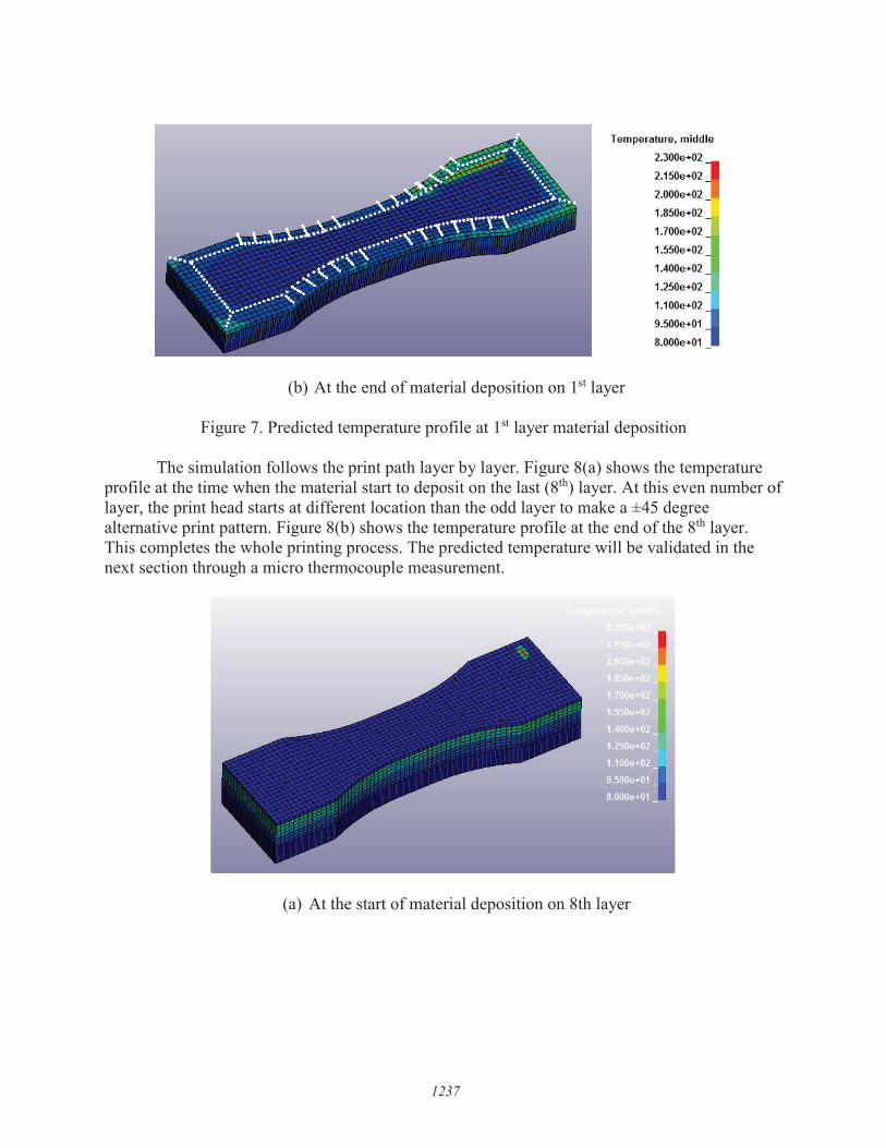
(b) At the end of material deposition on 1st layer

Figure 7. Predicted temperature profile at 1st layer material deposition

The simulation follows the print path layer by layer. Figure 8(a) shows the temperature profile at the time when the material start to deposit on the last (8th) layer. At this even number of layer, the print head starts at different location than the odd layer to make a ±45 degree alternative print pattern. Figure 8(b) shows the temperature profile at the end of the 8th layer. This completes the whole printing process. The predicted temperature will be validated in the next section through a micro thermocouple measurement.

(a) At the start of material deposition on 8th layer

1237

Temperature, middle

2.300e•02

2.150e•02

2.000e+02

1.850e+02

1.700e•02

1.550e•02

1.400e+02

1.250e+02

1.100e+02

9.500e•01

8.000e•01

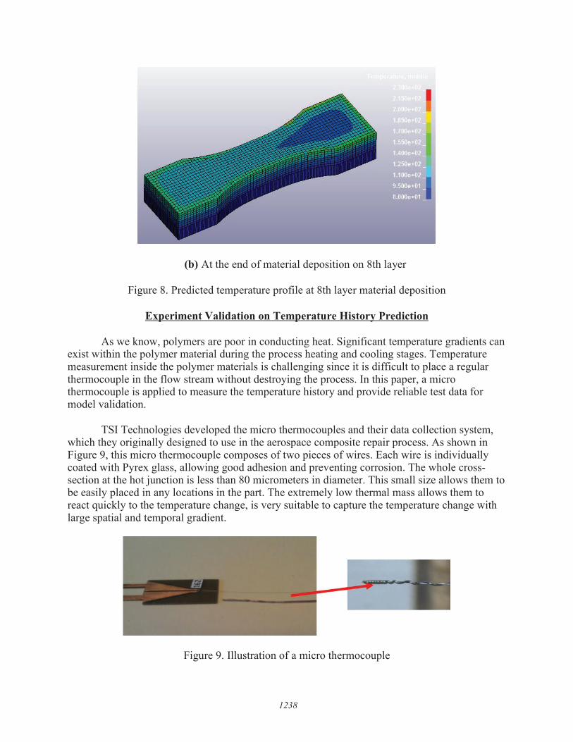
(b) At the end of material deposition on 8th layer

Figure 8. Predicted temperature profile at 8th layer material deposition

Experiment Validation on Temperature History Prediction

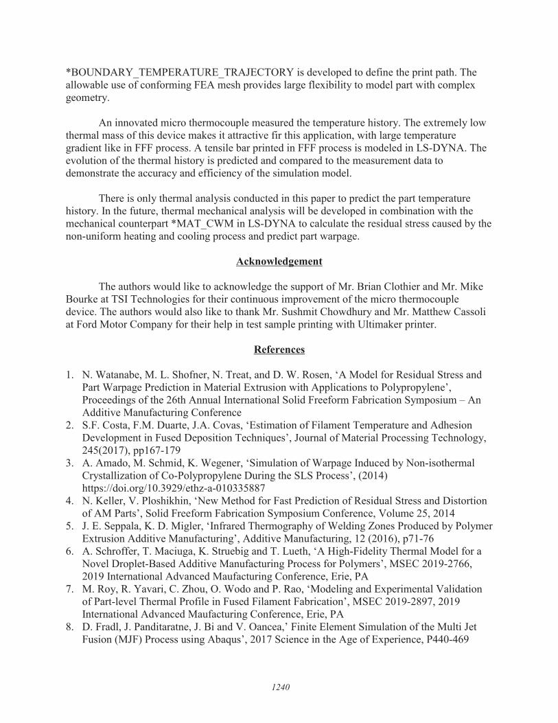
As we know, polymers are poor in conducting heat. Significant temperature gradients can exist within the polymer material during the process heating and cooling stages. Temperature measurement inside the polymer materials is challenging since it is difficult to place a regular thermocouple in the flow stream without destroying the process. In this paper, a micro thermocouple is applied to measure the temperature history and provide reliable test data for model validation.

TSI Technologies developed the micro thermocouples and their data collection system, which they originally designed to use in the aerospace composite repair process. As shown in Figure 9, this micro thermocouple composes of two pieces of wires. Each wire is individually coated with Pyrex glass, allowing good adhesion and preventing corrosion. The whole cross-section at the hot junction is less than 80 micrometers in diameter. This small size allows them to be easily placed in any locations in the part. The extremely low thermal mass allows them to react quickly to the temperature change, is very suitable to capture the temperature change with large spatial and temporal gradient.

Figure 9. Illustration of a micro thermocouple

1238

Validation: Result comparison between simulation and testing on the dog-bone sample

As shown in Figure 10, two micro thermocouples are located at the center of the tensile bar. During the printing process, they were positioned. One located between the fist layer and the glass build plate, the other placed between the second and third polymer layer. The size of the thermocouple is small enough that there is no effect when the print head passed by.

Figure 10. The placement of micro thermocouples in a printed tensile sample

Figure 11 shows the comparison of the temperature history between simulation and micro thermocouple measurement marked ‘1’ in Figure 10. All of the eight heating and cooling cycles during the printing of eight layer polymer are nicely captured. We can tell from the plot that the temperature drops sharply once the print head passed by.

Figure 11 Comparison of the temperature history between simulation and micro thermocouple measurement

Summary and future work

In this paper, an integrated approach is developed in LS-DYNA to model the FFF process and predict the temperature profile. A new keyword

1239

150 l - Mesured Data

u - Simulation QI

~ 130 0.0 QI

e. QI ... 3 110

~ QI Cl. E ~

70

0 50 100 150 200 250 300

Printing Time (s)

*BOUNDARY_TEMPERATURE_TRAJECTORY is developed to define the print path. The allowable use of conforming FEA mesh provides large flexibility to model part with complex geometry.

An innovated micro thermocouple measured the temperature history. The extremely low

thermal mass of this device makes it attractive fir this application, with large temperature gradient like in FFF process. A tensile bar printed in FFF process is modeled in LS-DYNA. The evolution of the thermal history is predicted and compared to the measurement data to demonstrate the accuracy and efficiency of the simulation model.

There is only thermal analysis conducted in this paper to predict the part temperature

history. In the future, thermal mechanical analysis will be developed in combination with the mechanical counterpart *MAT_CWM in LS-DYNA to calculate the residual stress caused by the non-uniform heating and cooling process and predict part warpage.

Acknowledgement

The authors would like to acknowledge the support of Mr. Brian Clothier and Mr. Mike Bourke at TSI Technologies for their continuous improvement of the micro thermocouple device. The authors would also like to thank Mr. Sushmit Chowdhury and Mr. Matthew Cassoli at Ford Motor Company for their help in test sample printing with Ultimaker printer.

References 1. N. Watanabe, M. L. Shofner, N. Treat, and D. W. Rosen, ‘A Model for Residual Stress and

Part Warpage Prediction in Material Extrusion with Applications to Polypropylene’, Proceedings of the 26th Annual International Solid Freeform Fabrication Symposium – An Additive Manufacturing Conference

2. S.F. Costa, F.M. Duarte, J.A. Covas, ‘Estimation of Filament Temperature and Adhesion Development in Fused Deposition Techniques’, Journal of Material Processing Technology, 245(2017), pp167-179

3. A. Amado, M. Schmid, K. Wegener, ‘Simulation of Warpage Induced by Non-isothermal Crystallization of Co-Polypropylene During the SLS Process’, (2014) https://doi.org/10.3929/ethz-a-010335887

4. N. Keller, V. Ploshikhin, ‘New Method for Fast Prediction of Residual Stress and Distortion of AM Parts’, Solid Freeform Fabrication Symposium Conference, Volume 25, 2014

5. J. E. Seppala, K. D. Migler, ‘Infrared Thermography of Welding Zones Produced by Polymer Extrusion Additive Manufacturing’, Additive Manufacturing, 12 (2016), p71-76

6. A. Schroffer, T. Maciuga, K. Struebig and T. Lueth, ‘A High-Fidelity Thermal Model for a Novel Droplet-Based Additive Manufacturing Process for Polymers’, MSEC 2019-2766, 2019 International Advanced Maufacturing Conference, Erie, PA

7. M. Roy, R. Yavari, C. Zhou, O. Wodo and P. Rao, ‘Modeling and Experimental Validation of Part-level Thermal Profile in Fused Filament Fabrication’, MSEC 2019-2897, 2019 International Advanced Maufacturing Conference, Erie, PA

8. D. Fradl, J. Panditaratne, J. Bi and V. Oancea,’ Finite Element Simulation of the Multi Jet Fusion (MJF) Process using Abaqus’, 2017 Science in the Age of Experience, P440-469

1240

9. LS-DYNA Manual R10.0, Volume II 10. F. Tiffaney, M. Gregory, and L. Todd, ‘Thermal Conductivity Testing Apparatus for 3D

Printed Materials’, ASME 2017 Summer Heat Transfer Conference, Bellevue, Washington, USA

11. S.C. Some, D. Delaunay, J. Faraj, J. Bailleul, N. Boyard, S. Quilliet, ‘Modeling of the thermal contact resistance time evolution at polymer–mold interface during injection molding: Effect of polymers' solidification’, Applied Thermal Engineering 84 (2015), pp 150-157

12. Thermal contact conductance, https://en.wikipedia.org/wiki/Thermal_contact_conductance

1241