Mechanics & Industry 17, 203 (2016)c© AFM, EDP Sciences 2016DOI: 10.1051/meca/2015071www.mechanics-industry.org

Mechanics&Industry

Numerical simulation of heat transfer in packed bedsby two population thermal lattice Boltzmann method

Robert Strakaa

Department of Heat Engineering and Environment Protection, Faculty of Metals Engineering and Industrial ComputerScience, AGH University of Science and Technology, Aleja Mickiewicza 30, 30-059 Cracow, Poland

Received 2 December 2014, Accepted 11 April 2015

Abstract – The Lattice Boltzmann Method (LBM) was used for simulation of a gas flow and conjugateheat transfer in fixed packed beds with solid particles inside. D2Q9 version of the Factorized CentralMoment (FCMLBM) is used for a gas flow computation. Heat transfer in the bed is described by seconddistribution function set and multiple relaxation time lattice Boltzmann method (DDF MRT LBM) isused. Numerical solver is implemented using NVIDIA CUDA framework and comparison of performanceon different GPUs is presented as well. Validation of the code is done using experimentally measured valuesof temperatures in fixed rock bed in a high-temperature thermal storage experiment. Next, the rate of heattransfer in a large scale fixed bed is numerically investigated, together with description of the bed’s thermalcharacteristics for two different mass flow rates of hot air.

Key words: Lattice Boltzmann method / packed bed / conjugate heat transfer

1 Introduction

Description of a conjugate heat transfer in packed bedsis of big interests in various branches of process industry(metallurgy, chemical, food processing, etc.). Our aim isto describe heat and fluid flow in shaft a furnace i.e. met-allurgical device used for rock melting. Models of shaftfurnaces are very rare in literature [1–3] (all those are only1D), it is due to the complicated load (randomly packed,nonspherical particles) geometry of such furnaces. Multi-ple granular materials resulting in variable porosity makefull numerical description of the problem problematic.Complex mesh generation when using standard numericalmethods like FDM, FEM or FVM in order to solve Navier-Stokes and Fourier-Kirchhoff equations is inevitable. Thenovel approach of solving those equations based on thediscrete version [4] of the Boltzmann transport equation iscalled the lattice Boltzmann method (LBM), it is provento be suitable for problems with complex geometry [5],thermal versions of LBM (TLBM) were successfully usedin different heat transfer problems [6–8] and due to ap-plication and optimization of code on GPUs [6, 8, 9], thismethod could deliver high performance numerical codesfor the heat transfer and fluid flow. During last decades,several approaches were developed, those are single relax-ation time (SRT) [4], multiple relaxation time (MRT) [10],

a Corresponding author: straka@metal.agh.edu.pl

entropic lattice Boltzmann method (ELBM) [11] and cas-caded lattice Boltzmann method (CLBM) [12]. All thesemethods have their advantages and drawbacks which canbe stated by the observation that the higher the stabilityof the approach is the higher the complexity and resourcesdemands are. Extensive review works on the state of theart LBM methods [5,13] exist together with several bookson this topic [4, 14–16].

Thermal LBMs can be generally divided to the threegroups. Multiple speed methods (one population modelwith extended set of characteristic velocities) [17], doubledistribution methods (treating temperature as a passivescalar) [18] and hybrid methods (using FDM, FEM orFVM to solve energy equation) [7]. Simple double dis-tribution method based on MRT was used, more ad-vanced double distribution models are described in ref-erences [19–21].

LBM with its stability, accuracy and robustness evenfor highly complicated meshes is very attractive whenconsidering basic problems in metallurgy which are basedon heat and mass transfer together with fluid flow in irreg-ular and porous structures like fixed or moving beds withchanging geometry of particles (e.g. due to combustion).Another attractive field of possible TLBM application inmetallurgy is numerical study of continuous steel cast-ing [22]. In material engineering, TLBM can be appliedin numerical investigation of heat transfer efficiency ofdouble finned radially twisted heat exchanger tubes with

Article published by EDP Sciences

R. Straka: Mechanics & Industry 17, 203 (2016)

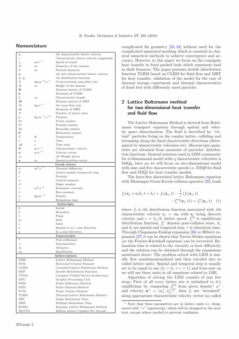
Nomenclature

ci ith characteristic lattice velocity

c Characteristic lattice velocity magnitude

cs m.s−1 Speed of sound

D m Diameter of the domain

d m Particle diameter

ei ith unit characteristic lattice velocity

fi, gi ith distribution function

G kg.m−2.s−1 Cross-sectional mass flow rate

H m Height of the domain

K Moment matrix of CLBM

k Moments of CLBM

L m Characteristic length

M Moment matrix of MRT

M kg.s−1 Air mass flow rate

m Moments of MRT

N Number of lattice sites

p kg.m−1.s−2 Pressure

Pe Peclet number

Pr Prandtl number

Re Reynolds number

S Relaxation matrix

T K Temperature

t s Time

Δt s Time step

U m.s−1 Characteristic velocity

u m.s−1 Velocity vector

wi ith Weight factor

x m Spatial position vector

Greek letters

α m2.s−1 Thermal diffusivity

δ Lattice spatial (temporal) step

ε Porosity

κ Central moment

Λ Magic number

ν m2.s−1 Kinematic viscosity

π Raw moment

ρ kg.m−3 Density

τ Relaxation time

Subscripts

0 Initial

b Boundary

f Fluid

in Inlet

s Solid

x Spatial or in x axis direction

y In y axis direction

Superscripts

* Post-collisional

+ Dimensionless

at Attractor

eq Equilibrium

Abbreviations

LBM Lattice Boltzmann Method

FCM Factorized Central Moment

CLBM Cascaded Lattice Boltzmann Method

DDF Double Distribution Function

CUDA Compute Unified Device Architecture

GPU Graphic Processing Unit

FDM Finite Difference Method

FEM Finite Element Method

FVM Finite Volume Method

TLBM Thermal Lattice Boltzmann Method

SRT Single Relaxation Time

MRT Multiple Relaxation Time

ELBM Entropic Lattice Boltzmann Method

MLUPS Million Lattice Updates Per Second

complicated fin geometry [23, 24] without need for thecomplicated numerical meshing which is essential in clas-sical numerical methods to achieve convergence and ac-curacy. However, in this paper we focus on the conjugateheat transfer in fixed packed beds which represents loadin shaft furnaces. The paper presents double distributionfunction TLBM based on CLBM for fluid flow and MRTfor heat transfer, validation of the model for the case ofthermal storage experiment and thermal characteristicsof fixed bed with differently sized particles.

2 Lattice Boltzmann methodfor two-dimensional heat transferand fluid flow

The Lattice Boltzmann Method is derived from Boltz-mann transport equation through spatial and veloc-ity space discretization. The fluid is described by “vir-tual” particles living on the regular lattice, colliding andstreaming along the fixed characteristic directions (deter-mined by characteristic velocities set). Macroscopic quan-tities are obtained from moments of particles’ distribu-tion functions. General notation used in LBM communityfor d-dimensional model with q characteristic velocities isDdQq, later on we will focus on two-dimensional modelwith nine and five characteristic speeds i.e. D2Q9 for fluidflow and D2Q5 for heat transfer models.

The force-free discretized lattice Boltzmann equationwith Bhatnagar-Gross-Krook collision operator [25] reads

fi(xj + ciδt, t + δt) = fi(xj , t) − 1τ

(fi(xj , t)

−f eqi (xj , t)) = f∗

i (xj , t) (1)

where fi is ith distribution function associated with ithcharacteristic velocity ci = cei with ei being discretevelocity and c = δx/δt lattice speed. f eq

i is equilibriumdistribution function, f∗

i denotes post-collision state, δx

and δt are spatial and temporal step, τ is relaxation time.Through Chapmann-Enskog expansion [26] or Hilbert ex-pansion [27] it can be shown that Navier-Stokes equations(or the Fourier-Kirchhoff equation) can be recovered. Re-laxation time is related to the viscosity or heat diffusivityand the relation can be obtained through the expansionsmentioned above. The problem solved with LBM is usu-ally first nondimensionalized and then rescaled into socalled lattice units. Spatial and temporal step is usuallyset to be equal to one (δt = δx = c = 1) and from now onwe will use these units in all equations related to LBE.

Algorithm of solving the LBM consists of just fewsteps. First of all every lattice site is initialized to it’sequilibrium by computing f eq

i from given density1 ρ+

and velocity u+ = (u+x , u+

y )T, then fi are “streamed”along appropriate characteristic velocity vector (so called

1 Note that these parameters are in lattice units i.e. desig-nated with “+” superscript, which will be dropped in the nexttext, except where needed to prevent confusion.

203-page 2

R. Straka: Mechanics & Industry 17, 203 (2016)

e0

e1

e2

e3 e4 e5

e6

e7e8

e0 e1

e2

e3

e4

Fig. 1. Characteristic velocities for D2Q9 (left) and D2Q5 (right) models.

streaming step), boundary conditions are set and newmacroscopic quantities are computed from fi, after thatcollision is performed i.e. relaxation towards equilibriumin case of BGK operator (so called collision step). Lastthree steps are repeated until desired time or steady stateis achieved.

The last ingredients here are the equation for the equi-librium distribution functions and relation between τ andν. Equilibrium distribution functions are given by Taylorexpansion of Maxwell’s distribution function [15]

f eqi = ρwi

(1 +

u · ei

c2s

+(u · ei)2

2c4s

− u · u2c2

s

)

where wi and cs are weight factors and lattice speed ofsound, they depend on the used lattice and on the setof characteristic velocities. Relaxation factor is related tofluid viscosity by

τ =ν

c2s

+12

Macroscopic density and velocities are given by followingmoments of fi:

ρ =∑

i

fi

ρu =∑

i

fiei

and pressure can be obtained by lattice equation of state

p = ρc2s

2.1 D2Q9 and D2Q5 model

In our numerical investigations the D2Q9 model wasused for fluid flow and D2Q5 for heat transfer. Set of char-acteristic velocities together with weighting factors andspeeds of sound is given below. Nine discrete velocities ofD2Q9 model are given by the set

[e0, . . . , e8] =(

0 1 −1 −1 0 1 1 1 00 −1 0 −1 −1 −1 0 1 1

)

with the set of weights

{w0, . . . , w8} ={

49,

136

,19,

136

,19,

136

,19,

136

,19

}

and the square of sound speed is equal to c2s = 1/3. Five

discrete velocities of D2Q5 model are given by the aboveset without diagonal vectors i.e.

{e0, . . . , e4} = {(0, 0); (1, 0); (0, 1); (−1, 0); (0,−1)}with the set of weights

{w0, . . . , w4} ={

13,16,16,16,16

}

and again the square of sound speed is equal to c2s = 1/3.

Equilibrium distribution function is defined as

geqi = Twi

(1 +

u · ei

c2s

)

Characteristic velocities within lattice site are depictedin Figure 1. Performing Chapmann-Enskog expansion, itcan be shown that for the case of the BGK D2Q9 [28]and D2Q5 models, following Navier-Stokes and Fourier-Kirchhoff equations can be recovered

∂ux

∂x+

∂uy

∂y= O(Ma2)

∂ux

∂t+

∂u2x

∂x+

∂uxuy

∂y= − ∂p

∂x+

1Re

[∂

∂x

(∂ux

∂x

)

+∂

∂y

(∂ux

∂y

)]+ O(Ma3)

∂uy

∂t+

∂uyux

∂x+

∂u2y

∂y= −∂p

∂y+

1Re

[∂

∂x

(∂uy

∂x

)

+∂

∂y

(∂uy

∂y

)]+ O(Ma3)

∂T

∂t+ ux

∂T

∂x+ uy

∂T

∂y= α

(∂2T

∂x2+

∂2T

∂y2

)+ O(Δt2) (2)

203-page 3

R. Straka: Mechanics & Industry 17, 203 (2016)

where Mach number is defined as Ma = |u|/cs and Δtis the time step in physical units (Δt = |U+|L/(|U|L+)where “+” denotes lattice units and U and L are charac-teristic velocity and length respectively).

2.2 Cascaded lattice Boltzmann method

To improve the stability of a SRT BGK model, ad-vanced MRT models were introduced and successfullyused till present time. However Geier et al. [12] realizedthat stability of MRT models can be improved drasticallywhen the Galilean invariance of MRT is restored. This isdone by performing the collision step in momentum spacewith central moments used in BGK operator instead ofraw ones. The main ideas of the CLBM will be brieflydescribed in this section.

Basic idea of MRT is performing collision step inmomentum space i.e. distribution functions vector f =(f0, . . . , fq−1)T is transformed by matrix M into mo-mentum space (m0, . . . , mq−1)T = m = Mf . Mo-ments are equilibrated towards their appropriate mo-mentum equilibria meq using diagonal matrix S =diag(1/τ0, . . . , 1/τq−1) i.e. with different relaxation times(MRT reduces to SRT when all τi are equal) and trans-formed back using inverse of M. The MRT LBE thereforereads

fi(xj+ei, t+1) = fi(xj , t)−M−1S (mi(xj , t) − meqi (xj , t))

We use transformation matrix given in [12] and denoteit K

K =

⎛⎜⎜⎜⎜⎜⎜⎜⎜⎜⎜⎜⎝

1 0 0 −4 0 0 0 0 41 −1 1 2 0 1 −1 1 11 −1 0 −1 1 0 0 −2 −21 −1 −1 2 0 −1 1 1 11 0 −1 −1 −1 0 −2 0 −21 1 −1 2 0 1 1 −1 11 1 0 −1 1 0 0 2 −21 1 1 2 0 −1 −1 −1 11 0 1 −1 −1 0 2 0 −2

⎞⎟⎟⎟⎟⎟⎟⎟⎟⎟⎟⎟⎠

next we define raw moments of fi as

πxmyn =∑

i

fiemi,xen

i,y

and central moments of fi as

κxmyn =∑

i

fi(ei,x − ux)m(ei,y − uy)n

where m, n ∈ Z and m + n is the order of the moment.The attractors for collision step are defined as

fat = f + K · k (3)

and central moments are computed for both sides of theEquation (3) i.e. we multiply it by (ei,x−ux)m(ei,y−uy)n

and take the sum over i. In result we obtain system of six

equations (first three moments are conserved quantitiesi.e. collisional invariants and thus not involved here) fork3, . . . , k8

⎛⎜⎜⎜⎜⎜⎝

6 2 0 0 0 06 −2 0 0 0 00 0 −4 0 0 0

−6uy −2uy 8ux −4 0 0−6ux −2ux 8uy 0 −4 0

8 + 6(u2x + u2

y) 2(u2y − u2

x) −16uxuy 8uy 8ux 4

⎞⎟⎟⎟⎟⎟⎠

·

⎛⎜⎜⎜⎜⎜⎝

k3

k4

k5

k6

k7

k8

⎞⎟⎟⎟⎟⎟⎠

=

⎛⎜⎜⎜⎜⎜⎝

κatxx − κxx

κatyy − κyy

κatxy − κxy

κatxxy − κxxy

κatxyy − κxyy

κatxxyy − κxxyy

⎞⎟⎟⎟⎟⎟⎠

If we set attractors to equilibrium i.e.⎛⎜⎜⎜⎜⎜⎜⎜⎜⎜⎜⎝

κatxx

κatyy

κatxy

κatxxy

κatxyy

κatxxyy

⎞⎟⎟⎟⎟⎟⎟⎟⎟⎟⎟⎠

=

⎛⎜⎜⎜⎜⎜⎜⎜⎜⎜⎜⎝

ρc2s

ρc2s

0

0

0

ρc4s

⎞⎟⎟⎟⎟⎟⎟⎟⎟⎟⎟⎠

and solve the above system, we obtain

k3 =1

12τ3

[ρ (u2

x + u2y) − f6 − f8 − f4 − f2 − 2 (f5 + f3

+f7 + f1 − ρc2s)

]k4 =

14τ4

[f8 + f4 − f6 − f2 + ρ(u2

x − u2y)

]

k5 =1

4τ5(f7 + f3 − f1 − f5 − uxuyρ)

k6 =−1τ6

{ [f5 + f3 − f7 − f1 − 2u2

xuyρ

+uy(ρ − f8 − f4 − f0)] /4

+ux

2(f7 − f1 − f5 + f3)

}+

uy

2(−3k3 − k4) + 2uxk5

k7 =−1τ7

{ [f3 + f1 − f5 − f7 − 2u2

yuxρ

+ux(ρ − f2 − f6 − f0)] /4

+uy

2(f7 − f1 − f5 + f3)

}+

ux

2(−3k3 + k4) + 2uyk5

k8 =14

[1τ8

(ρc4

s − κxxyy

) − 8k3 − 6k4(u2x + u2

y)

− 2k4(u2y − u2

x) + 16k5uxuy − 8k6uy − 8k7ux

]

for isotropic viscosity we set τ4 = τ5 = τ and compute τfrom

ν =1cs

(τ − 1

2

)

203-page 4

R. Straka: Mechanics & Industry 17, 203 (2016)

More accurate and stable version of CLBM, the Fac-torized Central Moment LBM was also proposed byGeier [29]. The only difference is in the attractor for the k8

k8 =14

[1τ8

(κat

xxyy − κxxyy

) − 8k3 − 6k4(u2x + u2

y)

− 2k4(u2y − u2

x) + 16k5uxuy − 8k6uy − 8k7ux

]

where κatxxyy is defined as

– κatxxyy = κeq

xxyy = ρc4s for CLBM

– κatxxyy = κ∗

xxκ∗yy for FCM

and post-collision states κ∗xx, κ∗

yy are given by

κ∗xx = 6k3 + 2k4 + κxx = 6k3 + 2k4 + πxx − ρu2

x

κ∗yy = 6k3 − 2k4 + κyy = 6k3 − 2k4 + πyy − ρu2

y

Now we can perform the collision step according to Equa-tion (3)

f(xj + ei, t + 1) = f + K · kto obtain distribution functions for the next time step.

2.3 MRT thermal lattice Boltzmann method

In order to simulate temperature field, the double dis-tribution function model is used i.e. we define second pop-ulation of distribution functions gi on the D2Q5 lattice.Temperature field is then simulated as a passive scalarobeying the advection-diffusion Equation (2). AssociatedMRT LBE for gi reads

gi(xj+ei, t+1) = gi(xj , t)−M−1S (mi(xj , t) − meqi (xj , t))

with matrices M and S defined as [30]

M =

⎛⎜⎜⎜⎝

1 1 1 1 10 1 0 −1 00 0 1 0 −14 −1 −1 −1 −10 1 −1 1 −1

⎞⎟⎟⎟⎠S = diag(0,

1τα

,1τα

,1τe

,1τν

)

and equilibrium moments given by

meq = (T, uxT, uyT, aT, 0)

to avoid “checkerboard” instabilities [31] we have to keepa < 1 and thermal diffusivity is then related to τα by

α =4 + a

10

(τα − 1

2

)

Additional constraints for other relaxation times are [31](

τe − 12

)=

(τν − 1

2

)and

(τα − 1

2

) (τν − 1

2

)= Λ

with Λ being the “magical number”. Those magical num-bers are selected to give special features of the MRT, someof them are [31]

– Λ = 14 best stability.

– Λ = 16 best diffusion, removes fourth order diffusion

error.– Λ = 1

12 best advection, removes third order advectionerror.

– Λ = 316 exact location of bounce back walls for

Poiseuille flow.

In our computations we used a = 2/3 together withΛ = 1/6 for solid and Λ = 1/12 for fluid lattice sites.Temperature is the only conserved quantity here and iscomputed as zeroth order moment of gi

T =∑

i

gi

2.4 Initial and boundary conditions

During initialization all lattice sites are setup to theequilibrium with the unit density, zero velocity and pre-scribed temperature T0

fi(xj , 0) = f eqi |ux=0,uy=0,ρ=1 gi(xj , 0) = geq

i |T=T0

Boundary conditions are needed at solid walls, inlets, out-lets and symmetry planes. Solid walls are treated withbounce-back boundary conditions located half-way, thatresults in no-slip conditions for velocity field and adia-batic conditions for the heat transfer

fi(xb, t + 1) = f∗i (xb, t)

where xb is boundary adjacent fluid site and fi corre-sponds to ei = −ei. In the case of a non-adiabatic fluid-solid interface no bounce-back is applied to the gi in orderto allow heat flowing through this interface. For inlet weuse the equilibrium conditions both for velocity and tem-perature fields i.e.

fi((0, Ny), t) = f eqi (ρin,uin) gi((0, Ny), t) = geq

i (Tin)

Outlet is modelled by first-order extrapolation

fi((Nx−1, j), t+1)=f∗i ((Nx−2, j), t) j ∈ [0, Ny[i ∈ 5, 6, 7

Finally, symmetry boundary conditions are realizedthrough mirroring the populations according to the sym-metry axis e.g. symmetry conditions for x axis symmetryare then defined by following relations

fi((j, 0), t + 1) = f ∗i ((j, 0), t) j ∈ [0, Nx[ i ∈ {1, 7, 8}

2.5 CUDA implementation of the solver

TLBM is implemented in C language and CUDA [32]framework is used in order to speed up the simulations.Common techniques of code optimization are used. Twocopies of lattice’s distribution functions are held in GPUmemory and accessed alternately i.e. only one kernel per-forming both collision and streaming step is needed. Data

203-page 5

R. Straka: Mechanics & Industry 17, 203 (2016)

Table 1. Average performance of the different kernels on GTXGPUs (in MLUPS).

kernel type Titan Z TitanIsothermal (FCMLBM) sp 2410 2162

Thermal (FCMLBM/MRT) sp 1281 1265Isothermal (FCMLBM) dp 1421 1351

Thermal (FCMLBM/MRT) dp 918 865

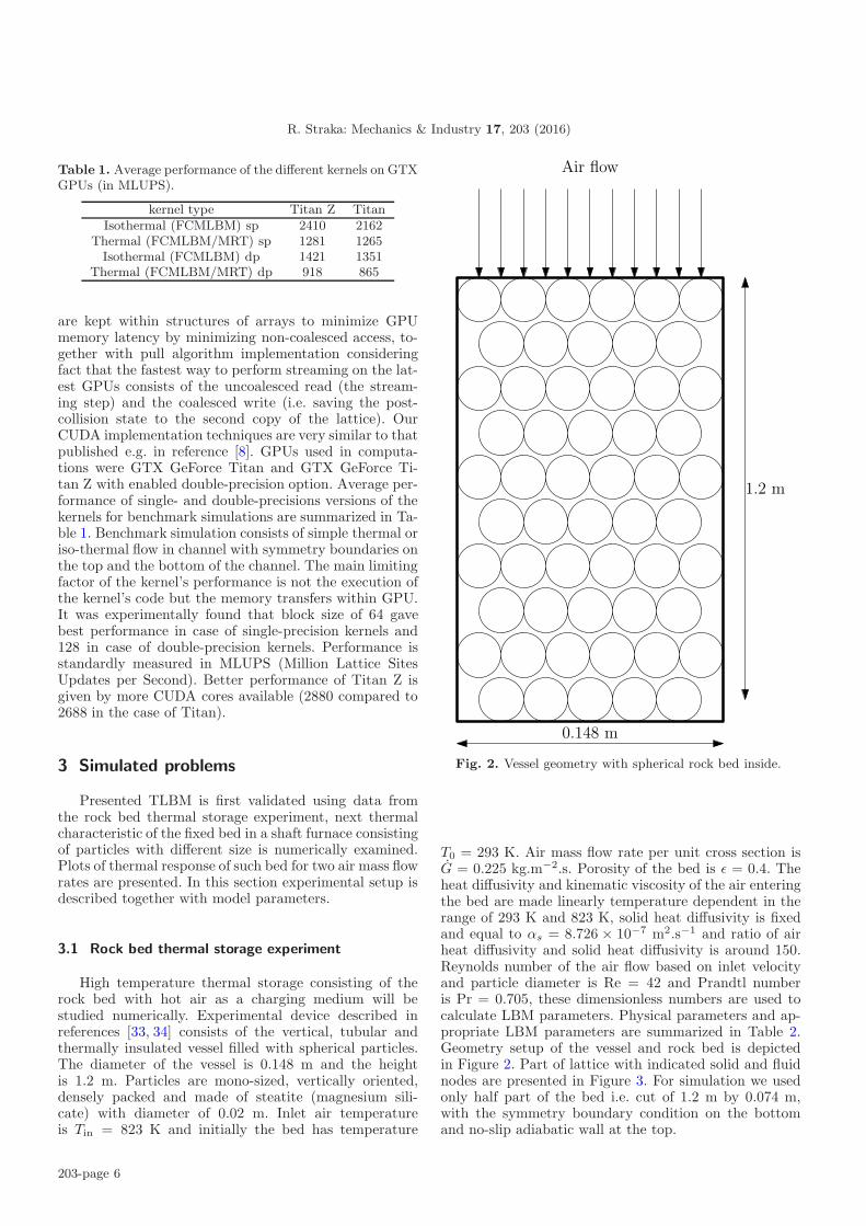
are kept within structures of arrays to minimize GPUmemory latency by minimizing non-coalesced access, to-gether with pull algorithm implementation consideringfact that the fastest way to perform streaming on the lat-est GPUs consists of the uncoalesced read (the stream-ing step) and the coalesced write (i.e. saving the post-collision state to the second copy of the lattice). OurCUDA implementation techniques are very similar to thatpublished e.g. in reference [8]. GPUs used in computa-tions were GTX GeForce Titan and GTX GeForce Ti-tan Z with enabled double-precision option. Average per-formance of single- and double-precisions versions of thekernels for benchmark simulations are summarized in Ta-ble 1. Benchmark simulation consists of simple thermal oriso-thermal flow in channel with symmetry boundaries onthe top and the bottom of the channel. The main limitingfactor of the kernel’s performance is not the execution ofthe kernel’s code but the memory transfers within GPU.It was experimentally found that block size of 64 gavebest performance in case of single-precision kernels and128 in case of double-precision kernels. Performance isstandardly measured in MLUPS (Million Lattice SitesUpdates per Second). Better performance of Titan Z isgiven by more CUDA cores available (2880 compared to2688 in the case of Titan).

3 Simulated problems

Presented TLBM is first validated using data fromthe rock bed thermal storage experiment, next thermalcharacteristic of the fixed bed in a shaft furnace consistingof particles with different size is numerically examined.Plots of thermal response of such bed for two air mass flowrates are presented. In this section experimental setup isdescribed together with model parameters.

3.1 Rock bed thermal storage experiment

High temperature thermal storage consisting of therock bed with hot air as a charging medium will bestudied numerically. Experimental device described inreferences [33, 34] consists of the vertical, tubular andthermally insulated vessel filled with spherical particles.The diameter of the vessel is 0.148 m and the heightis 1.2 m. Particles are mono-sized, vertically oriented,densely packed and made of steatite (magnesium sili-cate) with diameter of 0.02 m. Inlet air temperatureis Tin = 823 K and initially the bed has temperature

Air flow

0.148 m

1.2 m

Fig. 2. Vessel geometry with spherical rock bed inside.

T0 = 293 K. Air mass flow rate per unit cross section isG = 0.225 kg.m−2.s. Porosity of the bed is ε = 0.4. Theheat diffusivity and kinematic viscosity of the air enteringthe bed are made linearly temperature dependent in therange of 293 K and 823 K, solid heat diffusivity is fixedand equal to αs = 8.726 × 10−7 m2.s−1 and ratio of airheat diffusivity and solid heat diffusivity is around 150.Reynolds number of the air flow based on inlet velocityand particle diameter is Re = 42 and Prandtl numberis Pr = 0.705, these dimensionless numbers are used tocalculate LBM parameters. Physical parameters and ap-propriate LBM parameters are summarized in Table 2.Geometry setup of the vessel and rock bed is depictedin Figure 2. Part of lattice with indicated solid and fluidnodes are presented in Figure 3. For simulation we usedonly half part of the bed i.e. cut of 1.2 m by 0.074 m,with the symmetry boundary condition on the bottomand no-slip adiabatic wall at the top.

203-page 6

R. Straka: Mechanics & Industry 17, 203 (2016)

Table 2. Parameters of thermal storage experiment in physical and lattice units (denoted by “+”).

Physical units Lattice or no units

Tin 823 K T+in 1.0

T0 293 K T+0 0

H x D 1.2 × 0.148 m H+ × D+ 1200 × 74

d 0.02 m d+ 20

G 0.225 kg.m−2.s−1 Re 42

uin 0.187 m.s−1 u+ 0.12

ε 0.4 Pe 30

αf 1.249 × 10−4 m2.s−1 α+f 0.08015

ν 8.81 × 10−5 m2.s−1 ν+ 0.056536αf

αs∼150 Pr 0.705

Fig. 3. Detail of lattice (thin grid) structure with fluid (white)and solid (black) sites.

3.2 Conjugate heat transfer in packed bed

The large-scale fixed bed inside the shaft furnace withheight of 5.12 m and diameter equal to 2.56 m is filledup to 3/4 with double-sized spherical and non-sphericalparticles (see Fig. 4) with diameters 0.21 m and 0.11 m,irregularly packed with porosity equal to ε = 0.541. Hotair is blown inside at one side of the bed and leavingon the other like in the previous problem. Two differ-ent inlet velocities are considered u1,in = 0.0601 m.s−1

and u2,in = 0.1203 m.s−1 corresponding to the air massflows M1 = 0.4 kg.s−1 and M2 = 0.8 kg.s−1 at normalconditions. Other parameters like viscosity and thermaldiffusivities are kept same as in the previous simulationand are summarized together with other parameters inTable 3.

4 Results and discussion

Two numerical experiments were conducted in orderto test and validate presented TLBM for use in simula-tions of conjugate heat transfer and fluid flow in fixed

Hot air flow

2.56 m

5.12 m

T1

T2

T3

Fig. 4. Geometry setup of the second problem. Fixed bedof two different irregularly packed particles with free spaceabove the bed. Positions where temperature was measured aredenoted by arrows and numbers. Marked particles are used fortemperature history plots.

beds. In what follow the main results together with dis-cussions provided.

Area averaged bed temperatures along vertical direc-tion starting from the top are presented in Figure 5.

203-page 7

R. Straka: Mechanics & Industry 17, 203 (2016)

Table 3. Parameters used in packed bed conjugate heat transfer simulation in physical and lattice units (denoted by “+”).

Physical units Lattice or no units

Tin 823 K T+in 1.0

T0 293 K T+0 0

H x D 5.12 × 2.56 m H+ × D+ 512 × 256

d 0.21 m d+ 21

M1 0.4 kg.s−1 Pe1 101

u1,in 0.0601 m.s−1 Re1 143

M21 0.8 kg.s−1 Pe2 202

u1,in 0.1203 m.s−1 Re2 287

ε 0.54 u+ 0.1

αf 1.249 × 10−4 m2.s−1 α+1,f 0.02087

α+2,f 0.01038

ν 8.81 × 10−5 m2.s−1 ν+1 0.007324

ν+2 0.014659

αf

αs∼150 Pr 0.705

200

300

400

500

600

700

800

900

0 0.2 0.4 0.6 0.8 1 1.2 1.4

tem

pera

ture

[K]

distance [m]

average temp 1200saverage temp 3000saverage temp 4800s

exp 1200sexp 3000sexp 4800s

Fig. 5. Validation of the TLBM model using experimentaldata [34] for high temperature thermal storage vessel. Mea-sured temperatures for three time levels are marked with sym-bols, averaged computed temperature profiles are plotted asdashed lines.

Solid lines are computed temperature values and sym-bols denotes experimental values obtained from the liter-ature [34]. Three different time levels are compared. Over-all trend of measured temperature profiles is in very goodagreement with experimental values. Presented modeltends to under predict the temperature for later timesand lower half of the bed (note that we measure the dis-tance from the top of the vessel). Possible reason of this isvariable heat diffusivity of the bed material with temper-ature, although in model is kept fixed. Another possiblesource of errors are inaccuracies in temperature measure-ments during experiment and errors made during digitalprocessing of experimental data from [34]. Similar resultswere also obtained in reference [34] with 1D FDM modelconsisting of two energy conservation equations for fluidand solid phase. Based on the results we can say that

0

0.1

0.2

0.3

0.4

0.5

0.6

0.7

0 0.5 1 1.5 2 2.5

T+ [-

]

t+x10-5 [-]

T1T2T3

Fig. 6. Temperature history of bigger particles at three dif-ferent positions. Air mass rate M = 0.4 kg.s−1. Temperatureand time are in lattice units.

model is able to correctly predict conjugate heat flow infixed packed beds. In Table 4 computed and measured val-ues with absolute and relative errors for three time levelsare given. Maximal relative error is less than 7% and ten-dency of temperature under prediction by the model isclearly visible.

Second numerical experiment of conjugate heat trans-fer in large-scale fixed bed was performed for two valuesof hot air mass flow. Temporal profiles of temperature forbigger and smaller particles, together with temperatureof air in the vicinity of those particles are depicted inFigures 6–8 for the lower inlet speed and in Figures 9–11 for higher inlet speed. Temperature was collected nearthe bed’s centerline, in the middle of each particle, whichwas situated on three different vertical levels x1 = 1 m,x2 = 2 m and x3 = 3 m. Temperature, velocity magnitude(i.e.

√u2

x + u2y of real velocity not the superficial one) and

203-page 8

R. Straka: Mechanics & Industry 17, 203 (2016)

Table 4. Measured and computed values of average temperature with indicated absolute and relative errors.

Time Distance Measured Computed Absolute Relativein [s] in [m] temp. in [K] temp. in [K] error in [K] error in [%]1200 0.087 640.854 630.489 –10.364 –1.617

0.328 356.707 355.466 –1.242 –0.3480.512 301.829 309.388 7.559 2.5040.713 298.780 294.912 –3.869 –1.2950.909 296.951 293.085 –3.866 –1.3021.081 298.780 293.004 –5.777 –1.933

3000 0.087 796.341 794.203 –2.139 –0.2690.327 601.829 618.360 16.530 2.7470.512 409.756 424.159 14.403 3.5150.713 330.488 308.379 –22.108 –6.6900.909 304.268 293.610 –10.658 –3.5031.080 300.000 293.016 –6.984 –2.328

4800 0.087 809.146 803.269 –5.878 –0.7260.327 745.732 716.232 –29.500 –3.9560.513 596.341 610.626 14.284 2.3950.712 448.780 457.289 8.509 1.8960.908 359.756 345.484 –14.272 –3.9671.080 323.171 303.592 –19.579 –6.058

0

0.1

0.2

0.3

0.4

0.5

0.6

0.7

0.8

0.9

1

0 0.5 1 1.5 2 2.5

T+ [-

]

t+x10-5 [-]

T1T2T3

Fig. 7. Temperature history of smaller particles at three dif-ferent positions. Air mass rate M = 0.4 kg.s−1. Temperatureand time are in lattice units.

0

0.1

0.2

0.3

0.4

0.5

0.6

0.7

0.8

0.9

1

0 0.5 1 1.5 2 2.5

T+ [-

]

t+x10-5 [-]

T1T2T3

Fig. 8. Temperature history of air at three different positions.Air mass rate M = 0.4 kg.s−1. Temperature and time are inlattice units.

0

0.1

0.2

0.3

0.4

0.5

0.6

0.7

0.8

0 0.5 1 1.5 2 2.5 3 3.5 4 4.5

T+ [-

]

t+x10-5 [-]

T1T2T3

Fig. 9. Temperature history of bigger particles at three dif-ferent positions. Air mass rate M = 0.8 kg.s−1. Temperatureand time are in lattice units.

density (pressure) profiles for the last time step are shownin Figures 12 and 13 in dimensionless lattice units. Ef-fect of channeling is clearly visible in velocity plots. Ontemperature plots one can recognize slowly heating largerparticles with inner temperature gradient indicating highBiot number. From density profiles one can guess pressuredistribution and the pressure drop. Temporal behaviorof particles exhibits somewhat anomalous heating, whenparticles closer to inlet are first heated slowly than fartherparticles (see, e.g. Figs. 6, 7, 9 and 10). This can be ex-plained by channeling effect which causes higher convec-tive heat flux for distant particles due to higher velocitywhile the temperature of air is still almost the same asat the inlet. Temporal change of air temperatures is firstvery rapid (as hot air front is passing through the bed)and then slowly increasing (with visible spatial gradientof the air temperature) as particles are being heated up.

203-page 9

R. Straka: Mechanics & Industry 17, 203 (2016)

0

0.1

0.2

0.3

0.4

0.5

0.6

0.7

0.8

0.9

1

0 0.5 1 1.5 2 2.5 3 3.5 4 4.5

T+ [-

]

t+x10-5 [-]

T1T2T3

Fig. 10. Temperature history of smaller particles at three dif-ferent positions. Air mass rate M = 0.8 kg.s−1. Temperatureand time are in lattice units.

0

0.1

0.2

0.3

0.4

0.5

0.6

0.7

0.8

0.9

1

0 0.5 1 1.5 2 2.5 3 3.5 4 4.5

T+ [-

]

t+x10-5 [-]

T1T2T3

Fig. 11. Temperature history of air at three different posi-tions. Air mass rate M = 0.8 kg.s−1. Temperature and timeare in lattice units.

It is quite obvious that smaller particles are heated upfaster than bigger ones.

5 Conclusion

Thermal lattice Boltzmann model, based on doubledistribution function populations with factorized centralmoment method for fluid flow and multiple relaxationtime for heat transfer was presented. The validation of themodel was based on experimental data from literature [34]on high temperature thermal storage systems employingfixed packed bed of rocks with hot air as a heat transfermedium. The maximal relative error in the comparisonwas less than 7% and rather close to 2–3% with light un-der prediction of the measured temperatures. Next thethermal characteristics of irregularly packed large scalebed was conducted for packing of two types of sphericalparticles. Temporal characteristics of six different parti-cles at three different positions together with air temper-

Fig. 12. Instant profiles of density (top), velocity magnitude(middle) and temperature (bottom) in the last step of simula-tion for M = 0.4 kg.s−1 at the last time step t+ = 2.16 × 105

(t = 3600 s). Variables are plotted in lattice units.

Fig. 13. Instant profiles of density (top), velocity magnitude(middle) and temperature (bottom) in the last step of simula-tion for M = 0.8 kg.s−1 at the last time step t+ = 4.33 × 105

(t = 3600 s). Variables are plotted in lattice units.

ature in the vicinity of those particles were presented. In-stant snapshots of density, velocity and temperature fieldsare shown to reveal channeling effect in the porous struc-ture of the bed.

Acknowledgements. This work has been supported by the re-search Project No. 15.11.110.239 from the budget for scienceat Faculty of Metals Engineering and Industrial Computer Sci-ence, AGH University of Science and Technology.

203-page 10

R. Straka: Mechanics & Industry 17, 203 (2016)

References

[1] V. Stanek, B.Q. Li, J. Szekely, Mathematical Model of aCupola Furnace-Part I: Formulation and an Algorithm toSolve the Model, AFS Transactions 100 (1992) 425–437

[2] R. Leth-Miller, A.D. Jensen, P. Glarborg, L.M. Jensen,P.B. Hansen, P. B., S.B. Jørgensen, Investigation of amineral melting cupola furnace. Part II. Mathematicalmodeling, Indust. Eng. Chem. Res. 42 (2003) 6880–6892

[3] R. Straka, T. Telejko, 1D Mathematical Model of CokeCombustion, IAENG Int. J. Appl. Math. 45 (2015) 245–248

[4] S. Succi, The Lattice Boltzmann Equation for FluidDynamics and Beyond, Clarendon, Oxford, 2001

[5] D. Yu, R. Mei, L.S. Luo, W. Shyy, Viscous flow compu-tations with the method of lattice Boltzmann equation,Progress Aerospace Sci. 39 (2003) 329–367

[6] F. Kuznik, C. Obrecht, G. Rusaouen, J.J. Roux, LBMbased flow simulation using GPU computing processor,Comput. Math. Appl. 59 (2010) 2380–2392

[7] C. Obrecht, F. Kuznik, B. Tourancheau, J.J. Roux, TheTheLMA project: A thermal lattice Boltzmann solver forthe GPU, Comput. Fluids 54 (2012) 118–126

[8] N. Delbosc, J.L. Summers, A.I. Khan, N. Kapur,C.J. Noakes, Optimized implementation of the LatticeBoltzmann Method on a graphics processing unit to-wards real-time fluid simulation, Comput. Math. Appl.67 (2014) 462–475

[9] M.J. Mawson, A.J. Revell, Memory transfer optimiza-tion for a lattice Boltzmann solver on Kepler architec-ture nVidia GPUs, Comput. Phys. Commun. 185 (2014)2566–2574

[10] D. d’Humieres, I. Ginzburg, M. Krafczyk, P. Lallemand,L.S. Luo, Multiple-relaxation-time lattice Boltzmannmodels in three dimensions, Philos. Transa. R. Soc.London A 360 (2002) 437–51

[11] S.S. Chikatamarla, C.E. Frouzakis, I.V. Karlin, A.G.Tomboulides, K.B. Boulouchos, Lattice Boltzmannmethod for direct numerical simulation of turbulent flows,J. Fluid Mech. 656 (2010) 298–308

[12] M.C. Geier, Ab initio derivation of the cascaded lat-tice Boltzmann automaton, Ph.D. Thesis, University ofFreiburg, 2006

[13] C.K. Aidun, J.R. Clausen, Lattice-Boltzmann method forcomplex flows, Ann. Rev. Fluid Mech. 42 (2010) 439–472

[14] Z. Guo, C. Shu, Lattice Boltzmann method and itsapplications in engineering (advances in computationalfluid dynamics), World Scientific Publishing Company,Singapore, 2013

[15] A.A. Mohamad, Lattice Boltzmann Method, Springer-Verlag, London, 2011

[16] M.C. Sukop, D.T. Thorne Jr., Lattice BoltzmannModeling: An Introduction for Geoscientists andEngineers, Springer-Verlag, New York, 2006

[17] Y.H. Qian, Simulating thermohydrodynamics with latticeBGK models, J. Sci. Comput. 8 (1993) 231–242

[18] X. Shan, Simulation of Rayleigh-Benard convection us-ing a lattice Boltzmann method, Phys. Rev. E 55 (1997)2780–2788

[19] X. He, S. Chen, G.D. Doolen, A novel thermal model forthe lattice Boltzmann method in incompressible limit, J.Comput. Phys. 146 (1998) 282–300

[20] Z. Guo, C. Zheng, B. Shi, T.S. Zhao, Thermal latticeBoltzmann equation for low Mach number flows: decou-pling model, Phys. Rev. E 75 (2007) 036704

[21] I.V. Karlin, D. Sichau, S.S. Chikatamarla, Consistenttwo-population lattice Boltzmann model for thermalflows, Phys. Rev. E 88 (2013) 063310

[22] Z. Malinowski, M. Rywotycki, Modelling of the strandand mold temperature in the continuous steel caster,Arch. Civil Mech. Eng. 9 (2009) 59–73

[23] A. Szajding, T. Telejko, R. Straka, A. Goldasz,Experimental and numerical determination of heat trans-fer coefficient between oil and outer surface of monometal-lic tubes finned on both sides with twisted internal longi-tudinal fins, Int. J. Heat Mass Transfer 58 (2013) 395–401

[24] T. Telejko, A. Szajding, Heat exchange research of theboth side finned tubes applied to the heat exchangers,Rynek Energii 5 (2011) 104–110

[25] X. He, L.S. Luo, Theory of the lattice Boltzmann method:from the Boltzmann equation to the lattice Boltzmannequation, Phys. Rev. E 56 (1997) 6811–6817

[26] S. Chen, G.D. Doolen, Lattice Boltzmann method forfluid flows, Ann. Rev. Fluid Mech. 30 (1998) 329–364

[27] D. Hilbert, Mathematical problems, Bull. Am. Math. Soc.8 (1902) 437–479

[28] X. He, L.S. Luo, Lattice Boltzmann model for the incom-pressible Navier-Stokes equation, J. Stat. Phys. 88 (1997)927–944

[29] M.C. Geier, A. Greiner, J.G. Korvink, A factorized cen-tral moment lattice Boltzmann method, Eur. Phys. J.-Special Topics 171 (2009) 55–61

[30] H. Yoshida, N. Makoto, Multiple-relaxation-time latticeBoltzmann model for the convection and anisotropic dif-fusion equation, J. Comput. Phys. 229 (2010) 7774–7795

[31] I. Ginzburg, Truncation errors, exact and heuristic sta-bility analysis of two-relaxation-times lattice Boltzmannschemes for anisotropic advection-diffusion equation,Commun. Comput. Phys. 11 (2012) 1439–1502

[32] NVIDIA Corporation, NVIDIA CUDA C ProgrammingGuide v6.5, 2014

[33] A. Meier, C. Winkler, D. Wuillemin, Experiment for mod-elling high temperature rock bed storage, Solar EnergyMater. 24 (1991) 255–264

[34] M. Hanchen, S. Bruckner, A. Steinfeld, High-temperaturethermal storage using a packed bed of rocks-heat trans-fer analysis and experimental validation, Appl. ThermalEng. 31 (2011) 1798–1806

203-page 11