PHYSICAL REVIEW E 83, 046702 (2011)

Numerical simulation of asymptotic states of the damped Kuramoto-Sivashinsky equation

Hector Gomez* and Jose ParısUniversity of A Coruna, Campus de Elvina s/n, 15071, A Coruna, Spain

(Received 13 October 2010; revised manuscript received 21 February 2011; published 4 April 2011)

The damped Kuramoto-Sivashinsky equation has emerged as a fundamental tool for the understanding of theonset and evolution of secondary instabilities in a wide range of physical phenomena. Most existing studies aboutthis equation deal with its asymptotic states on one-dimensional settings or on periodic square domains. We utilizea large-scale numerical simulation to investigate the asymptotic states of the damped Kuramoto-Sivashinskyequation on annular two-dimensional geometries and three-dimensional domains. To this end, we proposean accurate, efficient, and robust algorithm based on a recently introduced numerical methodology, namely,isogeometric analysis.We compared our two-dimensional results with several experiments of directed percolationon square and annular geometries, and found qualitative agreement.

DOI: 10.1103/PhysRevE.83.046702 PACS number(s): 02.60.Cb, 02.70.−c

I. INTRODUCTION

A thermodynamical system far from equilibrium may ex-hibit primary instabilities which drive it into a inhomogeneousasymptotic state. In many relevant systems, these asymptoticstates consist of spatially and temporally ordered cellularstructures. In the past decades, there has been increasinginterest in the so-called secondary instabilities [1], which maydestroy the ordered cellular state, giving rise to disorderedstates both in space and time. Prime examples of phenomenawhere secondary instabilities exist are, for instance, theRayleigh-Benard convection [2,3], directional solidification[4,5], Faraday waves [6,7], or directed percolation [8–13]. Thetransition from a homogeneous stationary state to asymptoticcellular states through primary instabilities may be success-fully analyzed by using a linear stability analysis, but moresophisticated methods are necessary to understand secondaryinstabilities [14]. Remarkably, one of the most successful toolsfor the understanding of secondary instabilities has turnedout to be the study of the asymptotic states of the dampedKuramoto-Sivashinsky equation [15], which has emerged asa fundamental universal model describing the onset andevolution of secondary instabilities [14]. As a consequence,there is significant interest in the study of the asymptotic statesof the damped Kuramoto-Sivashinsky equation. The maindifficulty to achieve this goal is that the damped Kuramoto-Sivashinsky equation is not a gradient system [16]. Thus,there is no known Lyapunov functional for the equation. Thisfact significantly limits our capacity to study its asymptoticstates using analytical techniques, so a numerical simulationappears as a very attractive alternative. At this point, theone-dimensional equation is fairly well understood [15,17].In past years, significant progress has been made in theunderstanding of the two-dimensional equation [18], but theresults are limited to periodic square domains. Given the strongdependence of the asymptotic states on the geometry and thedimensionality of the domain [18,19], the understanding ofthe late-time states on nonsquare two- and three-dimensionaldomains is considered a very relevant research topic. This isprecisely one of the objectives of this work. To investigate the

*hgomez@udc.es

asymptotic states we use a numerical simulation. Thus, wepropose an effective, accurate, and robust numerical schemefor the damped Kuramoto-Sivashinsky equation, which isanother contribution of this work.

The numerical simulation of the damped Kuramoto-Sivashinsky equation presents several challenges. This is thereason why most calculations available in the literature arerestricted to one-dimensional settings [8,20–24] and onlyvery recently were two-dimensional simulations on squaredomains available [18,25–27]. We do not know of any three-dimensional simulation nor we are aware of two-dimensionalcalculations on nonsquare domains (although we know ofnumerical solutions to a modified Kuramoto-Sivashinskyequation on a disk [28–30]). We feel that one of the mainreasons for this is that the damped Kuramoto-Sivashinskyequation includes a fourth-order partial-differential operator.The numerical resolution of higher-order partial-differentialequations is significantly less developed than that of second-order problems. For example, in the context of finite-elementmethods, the use of conforming discretizations for fourth-orderpartial-differential spatial operators requires utilizing glob-ally C1-continuous basis functions. There exist some three-dimensional finite elements possessing global C1 continuity,but they introduce a number of additional degrees of freedomand severely restrict the geometrical complexity of the domain.Thus, in the finite-element context, the standard approach isto use a mixed method, which for a fourth-order problemdoubles the number of global degrees of freedom comparedto the primal variational formulation. As a consequence, themost widely used numerical methodologies for fourth-orderpartial-differential equations are either finite differences orpseudospectral collocation methods, whose applicability tocomplicated three-dimensional geometries is limited. Thus,we feel that there is no totally satisfactory solution to thehigher-order operator problem, yet fourth-order equations arebecoming ubiquitous, primarily due to the fast development ofphase-field modeling [31,32].

This work proposes a numerical formulation based onisogeometric analysis [33], which is a generalization offiniteelement analysis with several advantages [34–41]. Isoge-ometric analysis is based on developments of computationalgeometry and consists of using nonuniform rational B splines(NURBS) as basis functions in a variational formulation. For

046702-11539-3755/2011/83(4)/046702(11) ©2011 American Physical Society

HECTOR GOMEZ AND JOSE PARIS PHYSICAL REVIEW E 83, 046702 (2011)

(a) (b) (c)

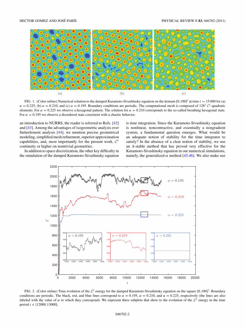
FIG. 1. (Color online) Numerical solution to the damped Kuramoto-Sivashinsky equation on the domain [0,100]2 at time t = 15 000 for (a)α = 0.225, (b) α = 0.210, and (c) α = 0.195. Boundary conditions are periodic. The computational mesh is composed of 1282 C1-quadraticelements. For α = 0.225 we observe a hexagonal pattern. The solution for α = 0.210 corresponds to the so-called breathing hexagonal state.For α = 0.195 we observe a disordered state consistent with a chaotic behavior.

an introduction to NURBS, the reader is referred to Refs. [42]and [43]. Among the advantages of isogeometric analysis overfiniteelement analysis [44], we mention precise geometricalmodeling, simplified mesh refinement, superior approximationcapabilities, and, most importantly for the present work, C1

continuity or higher on nontrivial geometries.In addition to space discretization, the other key difficulty in

the simulation of the damped Kuramoto-Sivashinsky equation

is time integration. Since the Kuramoto-Sivashinsky equationis nonlinear, noncontractive, and essentially a nongradientsystem, a fundamental question emerges. What would bean adequate notion of stability for the time integrator tosatisfy? In the absence of a clear notion of stability, we usean A-stable method that has proved very effective for theKuramoto-Sivashinsky equation in our numerical simulations,namely, the generalized-α method [45,46]. We also make use

0 2000 4000 6000 8000 10000 12000 14000 16000 18000 200000

200

400

600

800

1000

1200

1400

1600

1800

2000

2200

t

E

α = 0.225

α = 0.210

α = 0.195

12000 12200 12400 12600 12800 130001800

1850

1900

1950

2000

α = 0.195

12000 12200 12400 12600 12800 130001550

1600

1650

1700

1750

α = 0.210

12000 12200 12400 12600 12800 130001150

1200

1250

1300

1350

α = 0.225

FIG. 2. (Color online) Time evolution of the L2 energy for the damped Kuramoto-Sivashinsky equation on the square [0,100]2. Boundaryconditions are periodic. The black, red, and blue lines correspond to α = 0.195, α = 0.210, and α = 0.225, respectively (the lines are alsolabeled with the value of α to which they correspond). We represent three subplots that show to the evolution of the L2 energy in the timeperiod t ∈ [12000,13000].

046702-2

NUMERICAL SIMULATION OF ASYMPTOTIC STATES OF . . . PHYSICAL REVIEW E 83, 046702 (2011)

1217 1217.5 1218 1218.5 1219

−2

0

2

4

6

8

10x 10

−3

E

E

(a)

1591 1592 1593 1594 1595 1596 1597−1

−0.5

0

0.5

1

E

E

E

E

E

E(b)

1880 1890 1900 1910 1920 1930−10

−5

0

5

10

E

E

E

E

E

E

E

E

E

E

(c)

FIG. 3. (Color online) L2 energy phase planes for the damped Kuramoto-Sivashinsky equation on the square [0,100]2 for (a) α = 0.225,(b) α = 0.210, and (c) α = 0.195. Note that the vertical scales of the three subplots are different. The solid squares in the plots indicate wherethe phase planes start.

of an adaptive time-stepping algorithm to impose control overlocal errors [47].

Our space and time discretization schemes render aneffective, accurate, and robust methodology. We present two-dimensional numerical examples on nonsquare geometries andthree-dimensional simulations.

II. THE DAMPED KURAMOTO-SIVASHINSKY EQUATION

Here we state an initial and boundary-value problem for thedamped Kuramoto-Sivashinsky equation over the time interval[0,T ]. Let � ⊂ R3 be an open set. We denote � the boundary of�, which is assumed to have a continuous unit outward normalvector n. The problem is stated as follows: Given u0 : � �→ R,find u : � × [0,T ] �→ R such that

∂u

∂t= −�u − �2u − αu + |∇u|2 in � × (0,T ), (1)

u(x,0) = u0(x) in �, (2)

with adequate boundary conditions. Periodic boundary con-ditions are the standard choice in square domains. On morecomplex geometries the boundary conditions,

∇(u + �u) · n = 0, (3)

∇u · n = 0, (4)

may be utilized. In a variational formulation, Eqs. (3) and(4) may be thought of as natural boundary conditions for thedamped Kuramoto-Sivashinsky equation.

Although the dynamics of the Kuramoto-Sivashinsky equa-tion [48,49] is very complex, the four terms on the right-handside of Eq. (1) have a clear meaning in their own right. The firstterm is destabilizing in the sense that it increases the L2 energyin the system. Using the same terminology, we would qualifythe second and third terms as stabilizing. Finally, the last termis an energy-transfer operator. It transfers energy from lowerto higher frequencies [50].

Additional insight about primary instabilities of the equa-tion may be obtained by using a linear stability analysis

(a) (b)

FIG. 4. (Color online) Numerical solution to the damped Kuramoto-Sivashinsky equation on the square [0,512]2 at time t = 15 000 for (a)α = 0.225 and (b) detail of the solution. The plot on the right-hand side corresponds to the area marked with a box on the left-hand side. Theplots highlight the appearance of the penta-hepta defects experimentally observed in a pattern of two-dimensional jets [9].

046702-3

HECTOR GOMEZ AND JOSE PARIS PHYSICAL REVIEW E 83, 046702 (2011)

102

104

106

950

1000

1050

1100

1150

1200

1250

1300

1350

1400

1450

1500

α = 0.2400

α = 0.2375

α = 0.2350

α = 0.2325

α = 0.2300

α = 0.2275

α = 0.2250

τ

E

(a) Energy decay

0.225 0.23 0.235 0.24

6

7

8

9

10

11

12

13x 10

−5

α

<τ>

−1

(b) Stabilization time

FIG. 5. (Color online) On the left-hand side we plot the evolution of the L2 energy from a chaotic initial state to a stable state of constantenergy for seven values of α and different chaotic initial conditions. On the right-hand side we plot α vs the reciprocal of the average timebefore the system achieves a stable state of constant energy. The data fits a straight line with a coefficient of determination 0.9982.

[14]. It may be shown that the homogeneous constant stateu = 0 is linearly stable for α > 0.25. Additionally, it isknown that for α = 0 the Kuramoto-Sivashinsky equationleads to spatiotemporal chaotic states [51,52]. For intermediatevalues of α, the asymptotic states may be different. Oneof the most significant developments in past years is dueto Paniconi and Elder [18], who identified three asymptoticstates of the damped Kuramoto-Sivashinsky equation ona square domain for different values of α, namely, thehexagonally ordered (0.2176 < α < 0.2500), the so-calledbreathing hexagonal state (0.2070 < α < 0.2176), and thespatiotemporally chaotic (weakly turbulent) state (0 � α <

0.2070). Given the strong dependence of late-time states

on the dimensionality and topology of the domain, weaim at generalizing those results by performing numericalsimulations on two-dimensional nonsquare geometries andthree-dimensional calculations. The next section shows ourproposed numerical formulation to achieve this goal.

III. NUMERICAL FORMULATION

In this section we present our numerical formulation forthe damped Kuramoto-Sivashinsky equation. We first derivea semidiscrete formulation and then use an adaptive time-stepping method to advance the solution in time.

(a) (b) (c)

FIG. 6. (Color online) Numerical solution to the damped Kuramoto-Sivashinsky equation on an annular surface at t = 15000 for (a)α = 0.225, (b) α = 0.210, and (c) α = 0.195. Boundary conditions are defined in Eqs. (3) and (4). The computational mesh is composedof 256 elements in the circumferential direction and 64 in the radial direction. For α = 0.225 we observe a hexagonal pattern. The solutionfor α = 0.210 corresponds to the so-called breathing hexagonal state. For α = 0.195 we observe a disordered state consistent with a chaoticbehavior.

046702-4

NUMERICAL SIMULATION OF ASYMPTOTIC STATES OF . . . PHYSICAL REVIEW E 83, 046702 (2011)

0 2000 4000 6000 8000 10000 12000 14000 16000 18000 200000

100

200

300

400

500

600

700

800

900

1000

t

E

α = 0.225

α = 0.210

α = 0.195

12000 12200 12400 12600 12800 13000760

780

800

820

840

α = 0.195

12000 12200 12400 12600 12800 13000650

670

690

710

730

α = 0.210

12000 12200 12400 12600 12800 13000440

460

480

500

520

α = 0.225

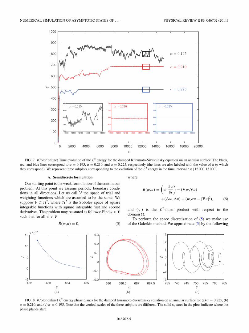
FIG. 7. (Color online) Time evolution of the L2 energy for the damped Kuramoto-Sivashinsky equation on an annular surface. The black,red, and blue lines correspond to α = 0.195, α = 0.210, and α = 0.225, respectively (the lines are also labeled with the value of α to whichthey correspond). We represent three subplots corresponding to the evolution of the L2 energy in the time interval t ∈ [12 000,13 000].

A. Semidiscrete formulation

Our starting point is the weak formulation of the continuousproblem. At this point we assume periodic boundary condi-tions in all directions. Let us call V the space of trial andweighting functions which are assumed to be the same. Wesuppose V ⊂ H2, where H2 is the Sobolev space of squareintegrable functions with square integrable first and secondderivatives. The problem may be stated as follows: Find u ∈ Vsuch that for all w ∈ V

B(w,u) = 0, (5)

where

B(w,u) =(

w,∂u

∂t

)− (∇w,∇u)

+ (�w,�u) + (w,αu − |∇u|2), (6)

and (·,·) is the L2-inner product with respect to thedomain �.

To perform the space discretization of (5) we make useof the Galerkin method. We approximate (5) by the following

482 483 484 485−5

0

5

10

15x 10

−3

E

E

(a)

686 686.5 687 687.5−0.2

−0.1

0

0.1

0.2

0.3

E

E

(b)

735 740 745 750 755 760 765−3

−2

−1

0

1

2

3

E

E

(c)

FIG. 8. (Color online) L2 energy phase planes for the damped Kuramoto-Sivashinsky equation on an annular surface for (a) α = 0.225, (b)α = 0.210, and (c) α = 0.195. Note that the vertical scales of the three subplots are different. The solid squares in the plots indicate where thephase planes start.

046702-5

HECTOR GOMEZ AND JOSE PARIS PHYSICAL REVIEW E 83, 046702 (2011)

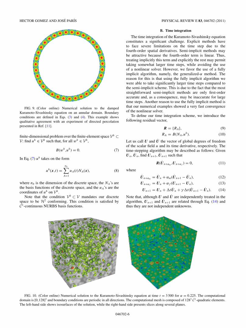
FIG. 9. (Color online) Numerical solution to the dampedKuramoto-Sivashinsky equation on an annular domain. Boundaryconditions are defined in Eqs. (3) and (4). This example showsqualitative agreement with an experiment of directed percolationpresented in Ref. [11].

finite-dimensional problem over the finite-element spaceVh ⊂V: find uh ∈ Vh such that, for all wh ∈ Vh,

B(wh,uh) = 0. (7)

In Eq. (7) uh takes on the form

uh(x,t) =nb∑

A=1

uA(t)NA(x), (8)

where nb is the dimension of the discrete space, the NA’s arethe basis functions of the discrete space, and the uA’s are thecoordinates of uh on Vh.

Note that the condition Vh ⊂ V mandates our discretespace to be H2 conforming. This condition is satisfied byC1-continuous NURBS basis functions.

B. Time integration

The time integration of the Kuramoto-Sivashinsky equationconstitutes a significant challenge. Explicit methods haveto face severe limitations on the time step due to thefourth-order spatial derivatives. Semi-implicit methods maybe attractive because the fourth-order term is linear. Thus,treating implicitly this term and explicitly the rest may permittaking somewhat larger time steps, while avoiding the useof a nonlinear solver. However, we favor the use of a fullyimplicit algorithm, namely, the generalized-α method. Thereason for this is that using the fully implicit algorithm wewere able to take significantly larger time steps compared tothe semi-implicit scheme. This is due to the fact that the moststraightforward semi-implicit methods are only first-orderaccurate and, as a consequence, may be inaccurate for largetime steps. Another reason to use the fully implicit method isthat our numerical examples showed a very fast convergenceof the nonlinear solver.

To define our time integration scheme, we introduce thefollowing residual vector,

R = {RA}, (9)

RA = B(NA,uh). (10)

Let us call U and U the vector of global degrees of freedomof the scalar field u and its time derivative, respectively. Thetime-stepping algorithm may be described as follows: GivenUn, Un, find Un+1, Un+1 such that

R(Un+αm,Un+αf

) = 0, (11)

where

Un+αm= Un + αm(Un+1 − Un), (12)

Un+αf= Un + αf (Un+1 − Un), (13)

Un+1 = Un + �tUn + γ�t(Un+1 − Un). (14)

Note that, although U and U are independently treated in thealgorithm, Un+1 and Un+1 are related through Eq. (14) andthus they are not independent unknowns.

FIG. 10. (Color online) Numerical solution to the Kuramoto-Sivashinsky equation at time t = 3 500 for α = 0.225. The computationaldomain is [0,128]3 and boundary conditions are periodic in all directions. The computational mesh is composed of 1283 C1-quadratic elements.The left-hand side shows isosurfaces of the solution, while the right-hand side presents slices along several planes.

046702-6

NUMERICAL SIMULATION OF ASYMPTOTIC STATES OF . . . PHYSICAL REVIEW E 83, 046702 (2011)

FIG. 11. (Color online) Numerical solution to the Kuramoto-Sivashinsky equation at time t = 3 500 for α = 0.210. The computationaldomain is [0,128]3 and boundary conditions are periodic in all directions. The computational mesh is composed of 1283 C1-quadratic elements.The left-hand side shows isosurfaces of the solution, while the right-hand side presents slices along several planes.

To complete the description of the method, it remainsto define αm, αf , and γ . These are real-valued parametersthat define the accuracy and the stability properties of thealgorithm. Jansen et al. [46] proved that, for a linear modelproblem, second-order accuracy is attained if

γ = 12 + αm − αf , (15)

while unconditional A stability requires

αm � αf � 1/2. (16)

We are interested in second-order accurate unconditionallyA-stable methods, so we will take values of αm, αf , and γ

that satisfy Eqs. (15) and (16) simultaneously. One of the keyfeatures of the generalized-α method is that αm and αf canbe parametrized in terms of ρ∞, the spectral radius of theamplification matrix that controls high-frequency dissipation[46]. Thus,

αm = 1

2

(3 − ρ∞1 + ρ∞

), αf = 1

1 + ρ∞. (17)

As a consequence, if we set ρ∞, and then select αm and αf

using (17) and calculate γ utilizing (15), we have a familyof second-order accurate unconditionally A-stable methodswith optimal control over high-frequency dissipation. Thedetails of the implementation of the generalized-α methodfor a nonlinear problem may be found in Ref. [47].

C. Time-step adaptivity

The undamped Kuramoto-Sivashinsky equation is known toamplify exponentially small perturbations in finite time inter-vals. For small values of the linear stabilizing term, the dampedequation retains this feature. Thus, accurate time integrationis key to perform reliable long-time computations. We feelthat these arguments recommend the use of adaptive time-stepcontrol. We employ a recently proposed adaptive algorithmthat can be used in conjunction with the generalized-α method.The details of this algorithm may be found in Ref. [47].

IV. NUMERICAL SIMULATIONS

In this section we present some two- and three-dimensionalnumerical examples. The purpose of these examples is three-fold: First, we aim at illustrating the effectiveness and ro-bustness of our numerical formulation; second, we investigatethe asymptotic states of the damped Kuramoto-Sivashinskyequation on nonsquare domains in two dimensions and oncubic three-dimensional domains; third, we compare oursimulations with directed percolation experiments.

Throughout this paper, for the computation of the asymp-totic states, we take as initial condition a random perturbationof the homogeneous state u = 0. The perturbations are directlyapplied to control variables and are uniformly distributed on[−0.05,0.05]. For the comparison with experiments we maytake different initial conditions that will be specified in eachcase.

For the space discretization we employ C1 quadraticNURBS for all the numerical examples.

A. Numerical simulations on a periodic square

1. Asymptotic states

Here we present the numerical solution to the dampedKuramoto-Sivashinsky equation on the domain � = [0,100]2.We use periodic boundary conditions and a computationalmesh composed of 1282 C1-quadratic elements. FollowingRefs. [18] and [25], we present simulations for α = 0.225,α = 0.210, and α = 0.195. Our results show the hexagonal(α = 0.225), breathing hexagonal (α = 0.210), and disordered(α = 0.195) states found by Paniconi and Elder [18]. Thehexagonal state is a spatially ordered stationary solution of thedamped Kuramoto-Sivashinsky equation found for relativelylarge values of α. The breathing hexagonal state is an unsteadysolution characterized by a quasiperiodic oscillation of thehexagonal pattern in which each cell oscillates out of phasewith its closest neighbor. In Fig. 1 we plot the numericalsolutions at time t = 15 000 for (a) α = 0.225, (b) α = 0.210,and (c) α = 0.195. To further illustrate the difference between

046702-7

HECTOR GOMEZ AND JOSE PARIS PHYSICAL REVIEW E 83, 046702 (2011)

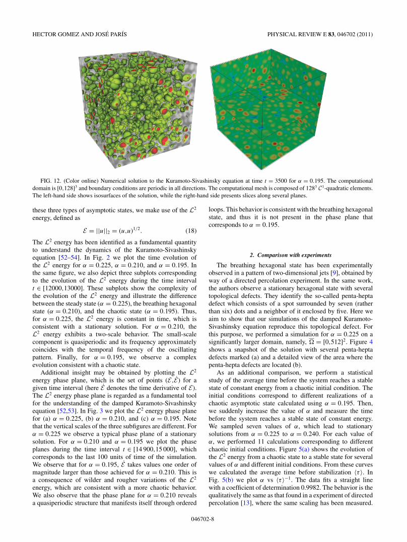
FIG. 12. (Color online) Numerical solution to the Kuramoto-Sivashinsky equation at time t = 3500 for α = 0.195. The computationaldomain is [0,128]3 and boundary conditions are periodic in all directions. The computational mesh is composed of 1283 C1-quadratic elements.The left-hand side shows isosurfaces of the solution, while the right-hand side presents slices along several planes.

these three types of asymptotic states, we make use of the L2

energy, defined as

E = ||u||2 = (u,u)1/2. (18)

The L2 energy has been identified as a fundamental quantityto understand the dynamics of the Kuramoto-Sivashinskyequation [52–54]. In Fig. 2 we plot the time evolution ofthe L2 energy for α = 0.225, α = 0.210, and α = 0.195. Inthe same figure, we also depict three subplots correspondingto the evolution of the L2 energy during the time intervalt ∈ [12000,13000]. These subplots show the complexity ofthe evolution of the L2 energy and illustrate the differencebetween the steady state (α = 0.225), the breathing hexagonalstate (α = 0.210), and the chaotic state (α = 0.195). Thus,for α = 0.225, the L2 energy is constant in time, which isconsistent with a stationary solution. For α = 0.210, theL2 energy exhibits a two-scale behavior. The small-scalecomponent is quasiperiodic and its frequency approximatelycoincides with the temporal frequency of the oscillatingpattern. Finally, for α = 0.195, we observe a complexevolution consistent with a chaotic state.

Additional insight may be obtained by plotting the L2

energy phase plane, which is the set of points (E,E) for agiven time interval (here E denotes the time derivative of E).The L2 energy phase plane is regarded as a fundamental toolfor the understanding of the damped Kuramoto-Sivashinskyequation [52,53]. In Fig. 3 we plot the L2 energy phase planefor (a) α = 0.225, (b) α = 0.210, and (c) α = 0.195. Notethat the vertical scales of the three subfigures are different. Forα = 0.225 we observe a typical phase plane of a stationarysolution. For α = 0.210 and α = 0.195 we plot the phaseplanes during the time interval t ∈ [14 900,15 000], whichcorresponds to the last 100 units of time of the simulation.We observe that for α = 0.195, E takes values one order ofmagnitude larger than those achieved for α = 0.210. This isa consequence of wilder and rougher variations of the L2

energy, which are consistent with a more chaotic behavior.We also observe that the phase plane for α = 0.210 revealsa quasiperiodic structure that manifests itself through ordered

loops. This behavior is consistent with the breathing hexagonalstate, and thus it is not present in the phase plane thatcorresponds to α = 0.195.

2. Comparison with experiments

The breathing hexagonal state has been experimentallyobserved in a pattern of two-dimensional jets [9], obtained byway of a directed percolation experiment. In the same work,the authors observe a stationary hexagonal state with severaltopological defects. They identify the so-called penta-heptadefect which consists of a spot surrounded by seven (ratherthan six) dots and a neighbor of it enclosed by five. Here weaim to show that our simulations of the damped Kuramoto-Sivashinsky equation reproduce this topological defect. Forthis purpose, we performed a simulation for α = 0.225 on asignificantly larger domain, namely, � = [0,512]2. Figure 4shows a snapshot of the solution with several penta-heptadefects marked (a) and a detailed view of the area where thepenta-hepta defects are located (b).

As an additional comparison, we perform a statisticalstudy of the average time before the system reaches a stablestate of constant energy from a chaotic initial condition. Theinitial conditions correspond to different realizations of achaotic asymptotic state calculated using α = 0.195. Then,we suddenly increase the value of α and measure the timebefore the system reaches a stable state of constant energy.We sampled seven values of α, which lead to stationarysolutions from α = 0.225 to α = 0.240. For each value ofα, we performed 11 calculations corresponding to differentchaotic initial conditions. Figure 5(a) shows the evolution ofthe L2 energy from a chaotic state to a stable state for severalvalues of α and different initial conditions. From these curveswe calculated the average time before stabilization 〈τ 〉. InFig. 5(b) we plot α vs 〈τ 〉−1. The data fits a straight linewith a coefficient of determination 0.9982. The behavior is thequalitatively the same as that found in a experiment of directedpercolation [13], where the same scaling has been measured.

046702-8

NUMERICAL SIMULATION OF ASYMPTOTIC STATES OF . . . PHYSICAL REVIEW E 83, 046702 (2011)

0 500 1000 1500 2000 2500 3000 3500 4000 4500 50000

500

1000

1500

2000

2500

3000

3500

4000

4500

5000

5500

t

E α = 0.225

α = 0.210

α = 0.195

2500 2550 2600 2650 2700 2750 28004700

4800

4900

5000

5100

α = 0.195

2500 2550 2600 2650 2700 2750 28003600

3700

3800

3900

4000

α = 0.210

2500 2550 2600 2650 2700 2750 28002750

2850

2950

3050

3150

α = 0.225

FIG. 13. (Color online) Time evolution of the L2 energy for the damped Kuramoto-Sivashinsky equation on the cube [0,100]3. Boundaryconditions are periodic in all directions. The black, red, and blue lines correspond to α = 0.195, α = 0.210, and α = 0.225, respectively (thelines are also labeled with the value of α to which they correspond). We represent three subplots corresponding to the evolution of the L2

energy in the time period t ∈ [2 500,2 800].

We remark that this scaling has also been observed in statisticalstudies of relaminarization in pipe or shear flows [55].

B. Numerical simulations on an annular surface

1. Asymptotic states

In this example we calculate the numerical solution tothe damped Kuramoto-Sivashinsky equation on an annularsurface. This geometrical setting has been very recentlyanalyzed under the assumption of radial symmetry [19]. Herewe remove this hypothesis. This example also shows that ournumerical formulation can be applied to nonsquare geometries,while maintaining its accuracy, stability, and robustness. Ourstudy suggests that the hexagonal, breathing hexagonal, anddisordered states found in the periodic square also exist in thisgeometrical setting.

The exterior radius of the annular surface is re = 50.0,while the interior is ri = 12.5. On the boundary, we imposethe conditions (3) and (4). We construct the computationalmesh joining four NURBS patches. Each of these patchescorresponds to a quarter of the annular surface and is composedof C1 quadratic NURBS elements. The patches are joint as tomaintain C1 continuity of the solution over the whole domain.This can be accomplished by applying linear restrictionoperators to the solution and weighting functions spaces. Theresulting mesh (comprising four patches) is composed of a totalof 256 elements in the circumferential direction and 64 in the

radial direction. We note that our formulation achieves exactgeometrical modeling of this problem. The reason for this isthat NURBS can represent all conic sections exactly [33].

In Fig. 6 we plot the solution for α = 0.225, α = 0.210,and α = 0.195 at time t = 15 000. To better understand theasymptotic states we make use again of the L2 energy timeevolution (see Fig. 7). The blue, red, and black lines correspondto α = 0.225, α = 0.210, and α = 0.195, respectively (seealso the labels appended to the lines). The dynamics of the L2

energy is qualitatively similar to the behavior exhibited in thelast example. In the subplots displayed in Fig. 7 we observethat for α = 0.225 the L2 energy is fairly constant, whichis consistent with a stationary solution. For α = 0.210 weobserve a quasiperiodic behavior, which is the manifestation ofthe breathing structure in theL2 energy. Finally, for α = 0.195,the plot shows a complex behavior consistent with a chaoticstate. This is again confirmed by the L2 energy phase planes,which are shown in Fig. 8. The phase plane for α = 0.225clearly corresponds to a stationary solution. For α = 0.210and α = 0.195 we plot the phase planes in the time intervalt ∈ [14 900,15 000], which corresponds to the last 100 unitsof time of the simulation. Observe that the vertical scales aredifferent for each subfigure. We note that for α = 0.195, Etakes values an order of magnitude larger than those takenfor α = 0.210. Also, for α = 0.210 there is a quasiperiodicstructure in the phase plane, which is not present for α =0.195. We conclude that the snapshots of the solution (Fig. 6)

046702-9

HECTOR GOMEZ AND JOSE PARIS PHYSICAL REVIEW E 83, 046702 (2011)

2850 2900 2950−15

−10

−5

0

5

10

15

20

E

E

(a)

3750 3800 3850 3900−15

−10

−5

0

5

10

15

20

E

E(b)

4800 4850 4900 4950−15

−10

−5

0

5

10

15

20

E

E

(c)

FIG. 14. (Color online) L2 energy phase planes for the Kuramoto-Sivashinsky equation on cube at the time interval t ∈ [3 400,3 500] for(a) α = 0.225, (b) α = 0.210, and (c) α = 0.195. Note that the vertical scale is the same for all subplots. The solid squares in the plots indicatewhere the phase planes start.

and the phase planes (Fig. 8) suggest that the asymptotic statesin the annular surface are the same as those found on theperiodic square, although this result may not hold if we changethe ratio of the exterior to the interior radii.

2. Comparison with experiments

The annular geometry has recently received the attentionfrom experimentalists both in the context of Rayleigh-Benardconvection [56] and directed percolation [11]. Here wecompare our numerical simulations with the experiementspresented in Ref. [11]. In particular, we show that the dampedKuramoto-Sivashinsky equation reproduces the transitionfrom a stationary liquid curtain to a pattern of columns,as predicted by the experiments. The annular geometry isdefined by an exterior radius re = 61 and a interior radiusri = 51. This geometry corresponds to one of the experimentspresented in Ref. [11]. The computational mesh is composedof 256 C1-quadratic elements in the circumferential directionand 16 elements in the radial direction. Boundary conditionsare defined by Eqs. (3) and (4). We simulate the stationaryliquid curtain by taking a constant initial condition u0(x) = 10.Then, we let the solution evolve until a pattern of columnsdevelops. Figure 9 shows the equilibrium arrangement, whichis in agreement with the cellular pattern found in Ref. [11].

C. Asymptotic states on three-dimensional domains

In this section we present the three-dimensional counterpartof the simulation presented in Sec. IV A 1. The computationaldomain is � = [0,100]3 and we employ a uniform meshcomposed of 1283 C1-quadratic elements. In this examplewe will not be able to run the calculations until such longtimes as in the two-dimensional simulations due to excessivecomputational cost. We ran the examples up to t = 3 500,which required ∼20 000 time steps. We assume that theasymptotic states are reached before this time. In Figs. 10,11, and 12 we plot the numerical solutions at time t = 3 500for α = 0.225, α = 0.210, and α = 0.195, respectively. On theleft-hand side of each figure we plot isosurfaces of the solution,while on the right-hand side we present slices along severalplanes, which clearly show disordered states. We also note that

there are no qualitative differences between the solutions fordifferent values of α. Figure 13 shows the evolution of the L2

energy for α = 0.225, α = 0.210, and α = 0.195. In all caseswe observe a complex evolution without a clear structure.Additionally, Fig. 13 shows that the trend in the evolution ofthe L2 energy is fairly constant from t = 300 until the endof the computation. This supports our hypothesis about theasymptotic states being reached before t = 3500. To furtheranalyze the evolution of theL2 energy we make use again of thephase planes, which are shown in Fig. 14. The phase planescorrespond to the last 100 units of time of the simulation.Unlike in the two-dimensional examples, the vertical scaleis the same for all subplots. We do not observe qualitativedifferences between the phase planes for the three values ofα. We conclude that, although further study is warranted, thesnapshots of the solution (Figs. 10–12) and theL2 energy phaseplanes (Fig. 14) suggest that the hexagonal and the breathinghexagonal states may not exist on three-dimensional domains.

V. CONCLUSION

We presented a computational approach to investigatethe asymptotic states of the damped Kuramoto-Sivashinskyequation. We applied our numerical technique to problems onnonsquare two-dimensional geometries and three-dimensionaldomains. Thus, our work extends previous studies on the topicwhich were almost invariably restricted to one-dimensionalsettings or square domains. Our study suggests that for thetwo-dimensional domain that we analyze the asymptotic statesare the same as those found on a periodic square. However,in three-dimensional domains we consistently found chaoticasymptotic states. Since the damped Kuramoto-Sivashinskyequation is a fundamental model that describes the onset andevolution of secondary instabilities, our study may contributeto a better understanding of physical phenomena exhibitingthis behavior. We presented several comparisons of our nu-merical simulations with experiments of directed percolation.We conclude that the damped Kuramoto-Sivashinsky equationreproduces the hexagonal and breathing hexagonal statesfound on directed percolation experiments on squares, and italso exhibits the penta-hepta defects found in experiments. We

046702-10

NUMERICAL SIMULATION OF ASYMPTOTIC STATES OF . . . PHYSICAL REVIEW E 83, 046702 (2011)

have also computed numerically the scaling of the stabilizationtime of chaotic solutions with respect to the control parameterα. Our study agrees qualitatively with an experiment ofdirected percolation. We have also presented a qualitativecomparison of our simulations with a directed percolationexperiment on an annular geometry.

ACKNOWLEDGMENTS

The authors were partially supported by Xunta de Galicia(Grants No. 09REM005118PR and No. 09MDS00718PR),Ministerio de Ciencia e Innovacion (Grants No. DPI2009-14546-C02-01 and No. DPI2010-16496) cofinanced withFEDER funds, and Universidad de A Coruna.

[1] M. C. Cross and P. C. Hohenberg, Annu. Rev. Fluid Mech. 22,143 (1990).

[2] S. W. Morris, E. Bodenshatz, D. S. Cannell, and G. Ahlers, Phys.Rev. Lett. 74, 391 (1995).

[3] H. W. Xi, J. D. Gunton, and J. Vinals, Phys. Rev. Lett. 71, 2030(1993).

[4] W. W. Mullins and R. F. Sekerka, J. Appl. Phys. 35, 444(1964).

[5] A. Valance, K. Kassner, and C. Misbah, Phys. Rev. Lett. 69,1544 (1992).

[6] N. B. Tufillaro, R. Ramshankar, and J. P. Gollub, Phys. Rev.Lett. 62, 422 (1989).

[7] W. Zhang and J. Vinals, Phys. Rev. Lett. 74, 690 (1995).[8] P. Brunet, Phys. Rev. E 76, 017204 (2007).[9] C. Pirat, C. Mathis, P. Maıssa, and L. Gil, Phys. Rev. Lett. 92,

104501 (2004).[10] C. Pirat, A. Naso, J.-L. Meunier, P. Maıssa, and C. Mathis, Phys.

Rev. Lett. 94, 134502 (2005).[11] C. Pirat, C. Mathis, M. Mishra, and P. Maıssa, Phys. Rev. Lett.

97, 184501 (2006).[12] P. Rupp, R. Richter, and I. Rehberg, Phys. Rev. E 67, 036209

(2003).[13] P. Brunet and L. Limat, Phys. Rev. E 70, 046207 (2004).[14] C. Misbah and A. Valance, Phys. Rev. E 49, 166 (1994).[15] H. Chate and P. Manneville, Phys. Rev. Lett. 58, 112 (1987).[16] L. M. Pismen, Patterns and Interfaces in Dissipative Dynamics

(Springer, Berlin, 2006).[17] K. R. Elder, J. D. Gunton, and N. Goldenfeld, Phys. Rev. E 56,

1631 (1997).[18] M. Paniconi and K. R. Elder, Phys. Rev. E 56, 2713 (1997).[19] A. Demirkaya and M. Stanislavova, Dynam. Part. Differ. Eq. 7,

161 (2010).[20] M. A. Lopez-Marcos, Appl. Numer. Math. 13, 147 (1993).[21] M. A. Lopez-Marcos, IMA J. Numer. Anal. 14, 233 (1994).[22] Y. Xu and C.-W. Shu, Comput. Method. Appl. Mech. 195, 3430

(2006).[23] D. Obeid, J. M. Kosterlitz, and B. Sandstede, Phys. Rev. E 81,

066205 (2010).[24] Y. H. Lan and P. Cvitanovic, Phys. Rev. E 78, 026208 (2008).[25] L. Cueto-Felgueroso and J. Peraire, J. Comput. Phys. 227, 9985

(2008).[26] S. Facsko, T. Bobek, A. Stahl, H. Kurz, and T. Dekorsy, Phys.

Rev. B 69, 153412 (2004).[27] J. T. Drotar, Y.-P. Zhao, T.-M. Lu, and G.-C. Wang, Phys. Rev.

E 59, 177 (1999).[28] P. Blomgren, S. Gasner, and A. Palacios, Chaos 15, 013706

(2005).[29] P. Blomgren, S. Gasner, and A. Palacios, Phys. Rev. E 72, 036701

(2005).

[30] P. Blomgren, A. Palacios, and S. Gasner, Math. Comput. Simul.79, 1810 (2009).

[31] A. J. Bray, Adv. Phys. 43, 357 (1994).[32] L. Q. Chen, Annu. Rev. Mater. Res. 32, 113 (2002).[33] J. A. Cottrell, T. J. R. Hughes, and Y. Bazilevs, Isogeometric

Analysis: Toward Integration of CAD and FEA (Wiley, Hoboken,NJ, 2009).

[34] I. Akkerman, Y. Bazilevs, V. M. Calo, T. J. R. Hughes, andS. Hulshoff, Comput. Mech. 41, 371 (2007).

[35] Y. Bazilevs, V. M. Calo, J. A. Cottrell, J. A. Evans, T. J. R.Hughes, S. Lipton, M. A. Scott, and T. W. Sederberg, Comput.Methods Appl. Mech. 199, 229 (2010).

[36] Y. Bazilevs, V. M. Calo, J. A. Cottrell, T. J. R. Hughes,A. Reali, and G. Scovazzi, Comput. Methods Appl. Mech. 197,173 (2007).

[37] Y. Bazilevs and T. J. R. Hughes, Comput. Mech. 43, 143 (2008).[38] J. A. Cottrell, T. J. R. Hughes, and A. Reali, Comput. Methods

Appl. Mech. 196, 4160 (2007).[39] J. A. Evans, Y. Bazilevs, I. Babuska, and T. J. R. Hughes,

Comput. Methods Appl. Mech. 198, 1726 (2009).[40] T. J. R. Hughes, J. A. Cottrell, and Y. Bazilevs, Comput. Methods

Appl. Mech. 194, 4135 (2005).[41] S. Lipton, J. A. Evans, Y. Bazilevs, T. Elguedj, and

T. J. R. Hughes, Comput. Methods Appl. Mech. 199, 357 (2010).[42] L. Piegl and W. Tiller, The NURBS Book, Monographs in Visual

Communication (Springer, Berlin, 1997).[43] D. F. Rogers, An Introduction to NURBS With Historical

Perspective (Academic, New York, 2001).[44] T. J. R. Hughes, The Finite Element Method: Linear Static and

Dynamic Finite Element Analysis (Dover, New York, 2000).[45] J. Chung and G. M. Hulbert, J. Appl. Mech. 60, 371 (1993).[46] K. E. Jansen, C. H. Whiting, and G. M. Hulbert, Comput.

Methods Appl. Mech. 190, 305 (1999).[47] H. Gomez, V. M. Calo, Y. Bazilevs, and T. J.

R. Hughes, Comput. Methods Appl. Mech. 197, 4333(2008).

[48] Y. Kuramoto and T. Tsuzuki, Prog. Theor. Phys. 55, 356 (1976).[49] G. I. Sivashinsky, Acta Astronom. 4, 1177 (1977).[50] M. Rost and J. Krug, Physica D 88, 1 (1995).[51] B. M. Boghosian, C. C. Chow, and T. Hwa, Phys. Rev. Lett. 83,

5262 (1999).[52] Y.-S. Smyrlis and D. T. Papageorgiou, Proc. Natl. Acad. Sci.

USA 88, 11129 (1991).[53] G. Akrivis and Y.-S. Smyrlis, Appl. Numer. Math. 51, 151

(2004).[54] L. Giacomelli and F. Otto, Commun. Pure Appl. Math. 53, 297

(2005).[55] S. Bottin and H. Chate, Eur. Phys. J. B 6, 143 (1998).[56] P. Berge, Nucl. Phys. B 2, 247 (1987).

046702-11