
Numerical Simulation of an Ekofisk Single Well Chemical ...
133
Numerical Simulation of an Ekofisk Single Well Chemical Tracer Test Mari Mikalsen Petroleum Geoscience and Engineering Supervisor: Jan-Åge Stensen, IPT Co-supervisor: Robert Moe, ConocoPhillips Department of Petroleum Engineering and Applied Geophysics Submission date: June 2014 Norwegian University of Science and Technology
Transcript of Numerical Simulation of an Ekofisk Single Well Chemical ...

Numerical Simulation of an Ekofisk Single Well Chemical Tracer Test
Mari Mikalsen
Petroleum Geoscience and Engineering
Supervisor: Jan-Åge Stensen, IPTCo-supervisor: Robert Moe, ConocoPhillips
Department of Petroleum Engineering and Applied Geophysics
Submission date: June 2014
Norwegian University of Science and Technology


___________________________________________________________________________

___________________________________________________________________________
I
Numerical Simulation of an Ekofisk
Single Well Chemical Tracer Test
___________________________________________________________________________
Master Thesis by
Mari Mikalsen
June 2014

___________________________________________________________________________
I

___________________________________________________________________________
II
Acknowledgements
This master thesis is the final part of the Master of Science program in Petroleum
Engineering at the Norwegian University of Science and Technology (NTNU). The thesis was
written in co-operation with ConocoPhillips Scandinavia AS. I would like to thank them for
the motivating and interesting project.
Next, I would like to thank Dr. Robert W. Moe for being my mentor at ConocoPhillips. I
would like to thank him for his excellent technical guidance, constructive support and
interesting discussions.
Also, I would like to thank Arvid Østhus for taking a special interest in my thesis; giving me
constructive feedback and guidance all the way through.
Thanks to Ole Eeg for his full support and assistance.
Further, I would like to thank my supervisor at NTNU, Jan Åge Stensen, for his support during
this thesis.
A special thanks to all the graduates at ConocoPhillips. Without all the lunch breaks, good
conversation and countless coffee breaks, I would have lost my mind.
Finally, I would like to thank my family and friends for the support and understanding during
the course of this thesis.

___________________________________________________________________________
III

___________________________________________________________________________
IV
Abstract
The Ekofisk field in the North Sea has been undergoing waterflood since 1987. It has proved
to efficiently recover oil by means of spontaneous imbibition. The plan is to continue
waterflooding until the end of the license in 2028. The challenge lies in how to recover the
residual oil left immobile after the waterflood. The average oil saturation in the flooded
parts of the reservoir is approximately 30 %. Surfactant flooding has now been proposed as
an option, and is showing promising results in the laboratory. An enhanced imbibition study
by injection of low concentration surfactants was conducted in the mid-1990s. The study
was terminated in 1997 due to lab measurements of unsatisfactory high adsorption, making
it un-economical. Further studies on surfactants were not done until 2011. The most
attractive feature of the surfactant this time around is its ability to lower IFT enough to free
immobile oil from the pores. Both the economics and understanding of the surfactant
process have improved significantly over the last 20 years, making it an option once again.
Current plans involve the implementation of a single well chemical tracer test in 2015 to
confirm the lab results on the effect the surfactant flood has on the residual oil. Several
simulation studies were conducted in this thesis to determine the expected injection rates
and the volumes necessary to execute an efficient pilot test. Particular attention is paid to
the influence of surfactant adsorption and the effect of geological features in the test area.
Adsorption proved to have a particular large effect on the acting distance of the surfactant
slug.
Based on history matching and other specific simulation studies, the expected injection rate
was determined to be 35 bbl/day for a 20 feet high perforation interval. With this rate a
total of 6 months to complete the SWCTT was required with the predetermined slug
volumes.

___________________________________________________________________________
V

___________________________________________________________________________
VI
Sammendrag
Ekofiskfeltet I Nordsjøen har blitt vannflømmet siden 1987. Det har vist seg å være svært
effektivt med tanke på å utvinne olje ved hjelp av spontan imbibering. Planen er å fortsette
vannflømmingen av feltet frem til lisensen går ut i 2028. Utfordringen ligger i hvordan å
utvinne den residuelle oljen som blir forlatt immobil i porene. Den gjennomsnittlige
oljemetningen i de flømmede områdene av reservoaret er omtrent 30 %. Surfaktant har nå
blitt foreslått som en mulighet, og viser lovende resultater fra kjerneflømminger. Et økt-
imbibering studie ved injeksjon av lav-konsentrasjon surfaktant ble utført på midten av
1990-tallet. Studiet ble avsluttet i 1997 etter at laboratoriemålinger viste utilfredsstillende
høye adsorpsjonsverdier som gjorde hele prosjektet uøkonomisk. Videre studier ble ikke
gjort før i 2011. Den mest attraktive egenskapen til surfaktanten i denne omgang var dens
evne til å redusere IFT nok til å frigjøre oljen fra porene. Både det økonomiske aspektet og
forståelsen av prosessen bak flømming med surfaktant har økt betraktelig i løpet av de siste
20 årene, og gjør det til et alternativ nok en gang.
Nåværende planer er å implementere en ènbrønns kjemisk tracer test i 2015 for å bekrefte
laboratorieresultatene om effekten surfaktant har på den residuelle oljemetningen. Flere
simuleringsstudier ble utført i denne oppgaven for å bestemme forventede injeksjonsrater
og nødvendige volumer for å gjennomføre en vellykket pilottest. Spesiell oppmerksomhet
ble rettet mot adsorpsjon av surfaktant og effekten av geologiske egenskaper i testområdet.
Adsorpsjon viste seg å ha en spesielt stor effekt på virkningslengden av surfaktanten.
Basert på historietilpasning og andre spesifikke simuleringsstudier, ble den forventede raten
bestemt til 35 bbl/dag for et 20 fots høyt perforeringsintervall. Med denne raten tok det
totalt 6 måneder å fullføre pilottesten med de forhåndsbestemte volumene.

___________________________________________________________________________
VII

___________________________________________________________________________
VIII
Table of Contents
1 Introduction .............................................................................................................. 1
2 Ekofisk Field History and Background ........................................................................ 3
2.1 Field Discovery ............................................................................................................. 3
2.2 Geology ........................................................................................................................ 4
2.3 Field Development....................................................................................................... 5
2.4 Subsidence ................................................................................................................... 7
2.5 Production from Chalk Reservoirs ............................................................................... 8
2.5.1 Water Weakening in Chalks ............................................................................... 11
2.6 EOR Screening for Ekofisk .......................................................................................... 12
3 Theory .................................................................................................................... 17
3.1 Rock Properties .......................................................................................................... 17
3.1.1 Porosity ............................................................................................................... 17
3.1.2 Permeability ....................................................................................................... 18
3.2 Fluid-Rock Interaction ............................................................................................... 20
3.2.1 Interfacial Tension .............................................................................................. 20
3.2.2 Wettability .......................................................................................................... 21
3.3 Relative Permeability ................................................................................................. 21
3.3.1 Pseudo Relative Permeability Curves ................................................................. 23
3.4 Saturation .................................................................................................................. 23
3.4.1 Spontaneous Imbibition ..................................................................................... 24
4 Literature ................................................................................................................ 27
4.1 Surfactant Flooding ................................................................................................... 27
4.1.1 Types of Surfactants ........................................................................................... 29
4.1.2 Microemulsion Phase Behavior .......................................................................... 30
4.1.3 Optimum Salinity for Ultralow IFT ..................................................................... 32
4.1.4 Surfactant Retention .......................................................................................... 33
4.2 Recent Advances in Surfactant EOR .......................................................................... 34
4.3 Environmental Regulations of EOR Chemicals .......................................................... 36
5 Factors Influencing Recovery ................................................................................... 39
5.1 Displacement efficiency and Volumetric sweep efficiency ....................................... 39
5.2 Recovery Factor ......................................................................................................... 41
6 The EOR Process in General ..................................................................................... 43

___________________________________________________________________________
IX
7 EOR Methods with Basis in Waterflooding ............................................................... 47
7.1 The Screening Criteria ................................................................................................ 47
7.2 Chemical EOR Methods ............................................................................................. 48
7.2.1 Polymer Flooding................................................................................................ 48
7.2.2 Alkaline Flooding ................................................................................................ 49
7.2.3 Low Salinity Waterflooding ................................................................................ 49
7.2.4 Smart Water ....................................................................................................... 50
7.2.5 Microbial EOR ..................................................................................................... 50
8 The Ekofisk Model ................................................................................................... 51
8.1 History Matching ....................................................................................................... 51
8.2 PSim ........................................................................................................................... 51
8.3 2D Homogenous Sector Model ................................................................................. 52
8.4 2D Ekofisk Sector Model ............................................................................................ 55
8.4.1 Grid Refinement ................................................................................................. 61
9 Single Well Chemical Tracer Test (SWCTT) ................................................................ 63
9.1 The Function of a SWCTT ........................................................................................... 63
9.2 Geological Effect on Tracer Curves ............................................................................ 65
9.2.1 Two Extreme Geological Base Cases ................................................................... 65
9.2.2 Introduction of a High Permeability Layer .......................................................... 68
9.2.3 The Effect of Active Wells in the Vicinity of the Test Area .................................. 71
10 Introducing Surfactants to the Model ...................................................................... 73
10.1 The Basic Logistics of a Surfactant Flood ................................................................. 73
10.2 Surfactant Flooding in a 2D Sector Model ............................................................... 74
10.2.1 Confined Test Area ............................................................................................. 75
10.2.2 Unconfined Test Area ......................................................................................... 76
10.2.3 Residual Oil Distribution ..................................................................................... 80
10.3 Surfactant Flooding in a 2D Radial Model ............................................................. 82
10.3.1 Flow Scheme to Determine Slug Volumes ......................................................... 82
11 Conclusion and Discussion .......................................................................................... 87
11.1 Future Work and Limitations ................................................................................. 91
12 References .............................................................................................................. 93
Appendices .................................................................................................................... 101

___________________________________________________________________________
X
List of Figures
2.1 Location and map of the Ekofisk Field (COPNO).............................................................3
2.2 Cross sectional view of the Ekofisk- & Tor Formation (COPNO Internal)........................4
2.3 Tectonic and Stylolite fractures (COPNO Internal).........................................................4
2.4 Current platforms on Ekofisk (COPNO Internal).............................................................6
2.5 Subsidence rates from 1992 – 2008 (COPNO Internal)...................................................7
2.6 Subsidence of the concrete wall around the storage tank (COPNO Internal).................8
2.7 Effect of NC on residual oil saturation (Ahmed & Meehan 2012).................................10
2.8 Illustration showing ion interaction at (A) low temp. & (B) high temp. (Austad
et al.2008)....................................................................................................................12
2.9 Ekofisk EOR target (COPNO Internal)…........................................................................13
2.10 Historical EOR studies & waterflood for Ekofisk (COPNO Internal)..............................14
3.1 Idealized matrix-fracture system (Warren & Root 1963).............................................19
3.2 Capillary equilibrium of a spherical cap (Tiab & Donaldson 2012)...............................20
3.3 Wettability at solid-fluid interface. (a) Water-wet (b) Neutrally-wet
(c)Oil-wet (Tiab & Donaldson2012)..............................................................................21
3.4 Typical water-oil relative permeability curves for (a) water-wet &
(b) oil-wet (Tiab & Donaldson 2012)………….…………………………………………………………....22
3.5 Two-phase relative permeability curves; water-oil system – imbibition......................24
3.6 Spontaneous and forced imbibition and drainage capillary pressure curves
(Morrow & Mason 2001)..............................................................................................25
4.1 Representation of an ASP flooding sequence (COPNO Internal)..................................28
4.2 Representation of (a) cationic surfactant and (b) anionic surfactant..................... .....29
4.3 Ternary diagram of microemulsion system (Healy & Reed 1974)........................... .....31
4.4 Salinity gradient (COPNO Internal)...............................................................................32
4.5 Discharge of red and black chemicals on the NCS (Miljødirektoratet 2013)................37
6.1 Oil resources and reserves for the 25 largest Norwegian oil fields (NPD)....................44
7.1 Comparison of sweep efficiency in water flooding & polymer flooding(Sheng 2012)..49
8.1 Two-phase relative permeability curves.......................................................................52
8.2 Fractional flow curves for the four scenarios of relative permeability data.................53
8.3 Saturation profile for high kro, low kro, high krw & low krw.......................................54

___________________________________________________________________________
XI
8.4 Saturation profile for low krw and high kro…...............................................................54
8.5 Water flooding sequence and pressure in C11, 1994-2012 (COPNO Internal)…..........55
8.6 Water saturation distribution in year 2001 for the 2D Ekofisk sector model…............56
8.7 Water saturation distribution in year 2006 for the 2D Ekofisk sector model…............56
8.8 Water saturation data from sector model and history file in year 2001…………..……….57
8.9 Water saturation data from sector model and history file in year 2006….………….…….57
8.10 Water saturation data from sector model and history file in year 2012…..……………….58
8.11 Pressure data from sector model and history file in 2001, 2006 and 2012…...............59
8.12 Water saturation plotted against time for C11 at a depth of 9773 feet…………………...59
8.13 Pressure plotted against time for C11 well at a depth of 9773 feet………………………….60
8.14 Pressure plotted against time for C11 at a depth of 9873 feet…..................................60
8.15 Location (grey area) and design of the grid refinement (right)………….…….……………….61
9.1 Tracer profiles for active (EtOH) and passive (EtAc) tracer (COPNO Internal)…...........64
9.2 Tracer maps for confined and unconfined test areas after 2 months of injection…..…66
9.3 Water injection rate plotted against time for confined and unconfined cases…..........66
9.4 Tracer curves for confined and unconfined cases……………………………………………………..67
9.5 Tracer curves – Comparison of 1 & 0.5 months of CW injection. Confined…................68
9.6 Tracer maps. Fracture with permeability 50 md, 200 md & 1000 md. Confined….......69
9.7 Tracer curves – Effect of fractures. Confined................................................................69
9.8 Tracer maps. Fracture with perm. 50 md, 200 md & 1000 md. Unconfined….............70
9.9 Tracer curves – Effect of fractures. Unconfined………………………………………….…………….70
9.10 Tracer maps for when wells are shut in and when wells are active. Confined……….….71
9.11 Tracer profiles for when wells are shut in and when wells are active. Confined….......72
9.12 Cumulative tracer when wells are shut in and when wells are active. Confined……..…72
10.1 So distribution after 2 months injection. (Ads=0.40 mg/g). Confined……………….……...76
10.2 So distribution after 2 months injection. (Ads=1.6 mg/g). Confined….........................76
10.3 So distribution after 2 months injection. (Ads=0.40 mg/g). Unconfined......................77
10.4 So distribution after 2 months injection. (Ads=1.6 mg/g). Unconfined….....................77
10.5 Water injection- & oil production rates with & without surfactant (confined)............78
10.6 Water injection- & oil production rates with & without surfactant (unconfined)........78
10.7 Relative permeability and the effect of decreasing water saturation..........................79
10.8 Relative permeability and the effect of low IFT conditions on water injectivity...........80

___________________________________________________________________________
XII
10.9 Model representation of the fluid distribution inside a core........................................81
10.10 Presumably the correct representation of the fluid distribution inside a core……….....81
10.11 So, salinity and SF conc. 6 feet from the well. (Ads=0.4 mg/g)....................................84
10.12 So, salinity and SF conc. 16 feet from the well. (Ads=0.4 mg/g)..................................85
10.13 Back produced tracer curve for 2D radial model..........................................................86
11.1 Breakthrough curves in a 1D flow in a sand column. After Bear (1972).......................88
11.2 Computed tracer curve and field data. (Deans et. al. 1973)…......................................89
11.3 Illustration of a flow chart for an EOR screening process (Schlumberger 2014)…….....92

___________________________________________________________________________
XIII

___________________________________________________________________________
XIV
List of Tables
7.1 The screening criteria (Taber et al. 1997)……………………………………………..…………………..47
10.1 Schedule for the SWCTT (Adsorption = 0.4 mg/g)……………………………………..……………..83

___________________________________________________________________________
0
XIIV

___________________________________________________________________________
1
1 Introduction
The petroleum industry in Norway is by far superior when it comes to creating value,
Government income and export value. The oil and gas industry has produced values of 9000
billion NOK since the start of oil production on the North Continental Shelf (NCS) (Force
Report 2011). Production has slowly decreased since the Norwegian oil production peaked in
year 2000, and action is needed to maintain production levels. According to NPD (Norwegian
Petroleum Directorate) the total production of oil and gas on the NCS was 226 MSm3 oil
equivalents in 2012. The decline in oil production was 8.5 % from the previous year, while
gas production increased with 13% during the same time period. The forecast is that
production will continue on the same level as 2012 towards 2020, and then decrease
towards 2030; with increasing gas production and decreasing oil production
(Miljødirektoratet 2013).
More than half of the world`s remaining oil exists in carbonate (chalk and limestone)
reservoirs (Zahid et al. 2010). The low permeability chalk reservoirs in the southern part of
the North Sea are characterized by intense fracturing caused by tectonic activities. They are
classified as naturally fractured reservoirs. Standard recovery methods yield a significantly
lower recovery in fractured chalk reservoirs compared to sandstone reservoirs. The potential
enhanced oil recovery target is accordingly higher (Ersland et al. 2010).
In this thesis the terms enhanced oil recovery (EOR) and improved oil recovery (IOR) are
defined in accordance with the Norwegian Petroleum Directorate (NPD). IOR is defined as
any processes applied to improve sweep efficiency to extract more of the mobile oil fraction.
EOR is defined as processes aiming to improve production by targeting the immobile part of
the oil.
The entire reservoir on the Ekofisk field is currently under waterflood, both vertically and
laterally. The current plan is to continue the water injection until end of license in 2028.
While waterflooding at Ekofisk has been a huge success, it is recognized that there is a large

___________________________________________________________________________
2
potential for EOR. ConocoPhillips is currently looking at several possible EOR options and the
possibility of moving towards a Single Well Chemical Tracer Test by 2015.
Single Well Chemical Tracer Tests are widely used in the oil industry as the first field pilot.
The method needs careful planning and the results can be challenging to interpretate.
Numerical simulation is used to help design the pilot and for understanding the pilot results.
Design parameters could include injection volumes and rates, volume needed in the back
production and the size of the pilot.
The main objective of this thesis is to provide input to the design of a field test and to make
sensitivity runs to estimate the impact of heterogeneity on the results by use of the
ConocoPhillips in-house simulator, PSim. Also, to build a 2D sector model and match the
Ekofisk waterflood for the selected injector-producer pair, use the model to run initial single
well chemical tracer test sensitivities and use the input and results from the 2D model in a
2D radial model and simulate a field test. Run a sensitivity study including impact of
fractures, flow out of zone, temperature, etc.
This thesis starts with an introduction to the Ekofisk field history and background. Further,
the theory of particular interest for surfactant flooding is presented. A literature review of
surfactant flooding is featured in the succeeding chapter. Next, factors influencing recovery
are discussed; followed by a general description the EOR process and different EOR
techniques.
The key part of the thesis starts with an introduction to the Ekofisk model, followed by a
chapter discussing the concepts of a single well chemical tracer test including a simulation
study. Further, simulation studies of surfactant flooding in a 2D sector model and a 2D radial
model are presented. Finally, conclusions, discussion and thoughts around future work and
limitations are brought forward.

___________________________________________________________________________
3
Figure 2.1 Location and map of the Ekofisk Field (COPNO Internal).
2 Ekofisk Field History and Background
The greater Ekofisk Area comprises of eight fields in the North Sea, of which four are shut-in;
Cod, West Ekofisk, Albuskjell and Edda. The four fields currently producing are Ekofisk,
Eldfisk, Tor and Embla. ConocoPhillips Skandinavia AS operates the Greater Ekofisk Area with
an ownership of 35.11 % in production license (PL) 018. The partners are Total E&P Norge AS
(39.90 %), Eni Norge AS (12.39 %), Statoil Petroleum AS (7.60 %) and Petoro AS (5.00%). The
PL018 license is currently valid until 2028 (ConocoPhillips n.d). In 2013 production from
Ekofisk accounted for 8.4% of the total oil production on the Norwegian Continental Shelf
(SSB 2014).
2.1 Field Discovery
Ekofisk was discovered in 1969 in Block 2/4, located in the Central Graben; south in the
Norwegian sector of the North Sea (Figure 2.1). This particular discovery came at a time
when companies had started to become discouraged after unsuccessful exploration;
abandoning the search in the area. Even after the discovery of Ekofisk, reactions were
negative because the reservoir consisted of chalky limestone. It was only after four subsea
completed wells were drilled in 1971 and showed promising results, that other companies
turned believers (Van den Bark & Thomas 1980).

___________________________________________________________________________
4
Figure 2.2 Cross sectional view of the Ekofisk Formation and the Tor Formation (COPNO Internal).
2.2 Geology
The Ekofisk field is an elongated anticline with the major axis running North-South, and
covering around 12 000 acres. It consists of two overlying chalk formations – Ekofisk (Danian
age) and Tor (Maastrichtian age) – separated by a tight zone below the lower Ekofisk
formation (Figure 2.2). Roughly two thirds of the 7.1 billion STB oil in place is located in the
Ekofisk formation (Hermansen et al. 2000). The tight zone is 50 feet thick, and forms an
impermeable barrier between the two formations in the major part of the field.
Communication between the two formations is limited to the highly fractured areas on the
crest (Hallenbeck et al. 1991). The top of the Ekofisk formation is located at a depth of 9 600
ft. Both formations have thicknesses varying between 300 and 500 ft.
The chalk is naturally fractured with matrix permeability up to 5 md, and with an effective
permeability near 100 md. The Ekofisk formation is dominated by tectonic fractures, while
most of the fractures in the Tor formation are stylolite-associated. The other two fracture
types dominating the Ekofisk field are irregular and healed fractures. Figure 2.3 shows the
two main types of fractures; tectonic and stylolite.
Figure 2.3 Tectonic (Left) and Stylolite (Right) fractures (COPNO Internal).

___________________________________________________________________________
5
The overlying Ekofisk formation has somewhat higher porosity than the underlying Tor
formation; respectively 30% to 48% against 30% to 40% (Sulak 1990). The initial reservoir
pressure was 7135 psia at a depth of 10 400 ft. The field originally contained undersaturated
volatile oil at a bubble point pressure of 5560 psia at an initial temperature of 268 °F
(Hermansen et al. 2000).
2.3 Field Development
The Ekofisk field was developed in stages. Exploration progressed simultaneously with
development plans; hence the conditions for development changed. The first stage was
started in 1971, and consisted of test production from the discovery well and three appraisal
wells. Reports from this phase stated that the reservoir was as good as, or even better than
first assumed. This gained the confidence needed to move on to phase II – drilling 30 new
wells from three platforms and installing production facilities to handle 300 000 STB/D
(Boyce 1972).
In 1974 production through permanent facilities was initiated. In addition to the three
drilling platforms, the field terminal platform and living quarters, and a one-million-barrel
concrete storage tank was installed. The storage tank allowed production to continue when
weather conditions prevented offshore loading. An oil pipeline to Teesside, England became
operational in 1975, and in 1977 a gas pipeline to Emden, Germany was a reality (Sulak
1990). Production peaked in October 1976 at 350 000 STB/D, before rapidly decreasing.
Based on positive results from laboratory studies and a water injection pilot, it was in 1983
decided to commence water injection into the Tor Formation. In 1987 water injection began
from the water-injection platform 2/4 K with an injection capacity of 375 000 BWPD and 30
well slots. A water injection pilot was also initiated into the Lower Ekofisk Formation, and
showed promising signs. 11 additional injectors and 16 producers were drilled in early 1990
to realize water injection into Lower Ekofisk. Further expansion was done, and water
injection capacity was raised to 500 000 BWPD. In 1992 it was decided to start water

___________________________________________________________________________
6
injection into the Upper Ekofisk Formation as well, and water injection capacity was further
increased to 820 000 BWPD by use of a converted drilling rig.
Figure 2.4 shows the platforms and drilling rigs currently operating on Ekofisk. In addition to
the surface facilities, two subsea installations – Victor Alpha and Victor Bravo – are installed.
During the last 40 years of production, more than 400 wells have been drilled (COPNO
Internal).
In 1987, prior to the implementation of the waterflood, oil production rates were as low as
70 000 STB/D. In March 1990 the response from the waterflood was characterized by sharply
increased oil rates, declining GOR and low water cuts. The average water injection into
Ekofisk was as of March 2014 just below 400 000 BPD, divided between 32 active injectors.
As of March 2014 the oil production rates from Ekofisk were approximately 140 000 STB/D
(COPNO Internal).
Only 18% of the original oil in place (OOIP) in the Ekofisk field was initially estimated to be
recoverable. The discovery of reservoir compaction increased this primary recovery estimate
to 24%, because it led to increased recovery by compaction drive (Sulak 1990). In year 2000
the oil recovery estimate from Ekofisk was 38 % of the OOIP (Hermansen et al. 2000). As of
2014 an estimated recovery factor of 51 % seems possible by 2029 (COPNO Internal).
Figure 2.4 Current platforms on Ekofisk (COPNO Internal).

___________________________________________________________________________
7
Figure 2.5 Subsidence rates from 1992 – 2008 (COPNO Internal).
2.4 Subsidence
Seabed subsidence at the Ekofisk field was discovered in 1984. This was a result of reservoir
compaction from hydrocarbon extraction, leading to a massive decline in reservoir pressure.
Decreased pore pressure lead to an increase in effective stress, causing the weak chalk to
compact by pore collapse. It was first thought that natural conditions had caused the sea
level to rise, and the subsidence was not taken seriously. The belief at the time was that
compaction of the reservoir would lead to decreased productivity, and since productivity
was not decreasing, the reservoir could not be compacting. By 1984 the seabed beneath the
Ekofisk complex had subsided by more than 10 feet, and measurements confirmed that the
platforms were indeed sinking (Sulak 1990). Figure 2.5 shows the seabed subsidence rates
from year 1992 to 2008 for the hotel (red), the Ekofisk Alpha platform (green) and the
Ekofisk Bravo platform (blue).
The main problem and concern regarding the subsidence was the protection of the
platforms and the storage tank. The solution to secure the concrete tank was to build a
protective barrier around it. Figure 2.5 shows pictures of the protective wall around the
storage tank in years 1974, 1985 and 2006, and the degree of subsidence. The holes in the
wall are 1.3 meters for scale. For the platforms, a major jack up project was executed during
the summer of 1987. At the time the Ekofisk Center Complex consisted of six steel platforms
and inter-connected bridges; all elevated 6 meters to be out of harm’s way from storm
waves.

___________________________________________________________________________
8
Figure 2.6 Subsidence of the concrete protective wall around the storage tank (COPNO Internal).
The field wide water injection process has slowed down the subsidence rate. The decreasing
subsidence trend indicates good pressure support by the injected water. Although the
Ekofisk formation has been repressurized to a pressure greater than the bubble point of oil,
subsidence will continue with a rate of 15 cm/year in the water flooded areas. Estimated
subsidence by 2050 is 12 – 16 meters (COPNO Internal). The reason will be discussed in
subchapter 2.5.1. Compaction and subsidence are also issues for well integrity. There is great
well failure potential involved in the process of compaction; e.g. buckling of the wellbore. A
consequence of well collapse is that the process of P&A (Plug & Abandonment) of a well
becomes highly more difficult to implement. Seabed pipelines are also at risk when the
compaction leads to seabed subsidence.
2.5 Production from Chalk Reservoirs
The average recovery factor (RF) for carbonate reservoirs is far less than for sandstone
reservoirs. The worldwide RF for carbonate reservoirs is only 30%. Most of the reservoirs are
highly fractured, and almost 90% are oil-wet to neutral-wet; prohibiting oil displacement by
spontaneous imbibition of water. Contrary to sandstone behavior, carbonate reservoirs
appear to become increasingly oil-wet as the reservoir temperature decreases (Austad et al.
2008).

___________________________________________________________________________
9
In the North Sea the dominant oil-containing carbonate formation is chalk. The early
invasion of oil into these chalks is the reason for the natural fracture system and high
porosity. The Ekofisk chalk is very poorly cemented between grains. The main production
mechanism for fractured chalk reservoirs undergoing waterflood is spontaneous imbibition.
The imbibition process is affected by several parameters; rock characteristics (porosity,
permeability), fluid properties (density, viscosity and interfacial tension), wettability,
thermodynamic conditions, initial saturations and boundary conditions. Wettability varies
through the Ekofisk field. The Tor formation is water-wet, while conditions for the Lower and
Upper Ekofisk formations are mixed-wet to nearly oil-wet. Because of this, the nature of
spontaneous water imbibition is different for the formations (Austad & Milter 1997).
The injection of seawater proved to imbibe efficiently into the Ekofisk and Tor chalk matrix;
regardless of the low matrix permeability. The most crucial wetting parameter for
carbonates is the acid number, AN. The acid number represents the amount of carboxylic
acids present in the crude oil. At natural pH the initial interface between chalk and water is
positively charged, while the interface between oil and water is negatively charged. Thus,
the disjoining pressure in the water film becomes negative, and oil contacts the chalk
surface; making it naturally oil-wet (Austad et al. 2008).
Cuiec et al. (1994) established the importance of capillary forces and the existence of a
predominant countercurrent mechanism at constant and high interfacial tension (IFT). Their
research concluded that as IFT was lowered, the final recovery increased. A chalk core
experiment showed that the water volume imbibed into a given end was equal to the oil
volume produced by the same end. It was confirmed that the oil was produced by
countercurrent flows into the fractures, and that no cocurrent flow occurred during
spontaneous imbibition. At high IFT`s (41 mN/m) no additional oil was displaced when a
forced imbibition was performed after a spontaneous imbibition, confirming that no mobile
oil was trapped in the core after the process (Cuiec et al. 1994).
Capillary forces are the main driving forces in spontaneous imbibition. The capillary number,
NC, expresses the ratio of viscous to capillary forces, and is given in eq.2.1;

___________________________________________________________________________
10
Figure 2.7 Effect of NC on residual oil saturation (Ahmed & Meehan 2012).
Where µ is the fluid viscosity, V is the fluid velocity and σ the interfacial tension. In forced
displacements the goal is to mobilize the residual oil saturation. This can be done by
lowering the IFT to raise the capillary number enough to overcome the capillary forces.
Viscous forces will then dominate, and allow oil to flow. The capillary number has to exceed
the critical capillary number in order to mobilize residual oil. The relationship is illustrated by
the graph in Figure 2.7;
In water-wet chalks the fluid flow is countercurrent at high IFT; governed by capillary forces.
At low IFT (0.02 mN/m) imbibition goes from being capillary dominated to being gravity
dominated. The oil production in the gravity dominated regime is slow compared to the
production driven by capillary forces. At low IFT a larger fraction of the oil is produced by the
slow gravity process. For field applications this may mean too long of a delay. The crossover
point from capillary forced imbibition to gravity dominated imbibition can be scaled
according to the inverse Bond number, NB-1, which is the ratio between capillary and gravity
forces;
Where C is a constant related to pore geometry, σ is the interfacial tension, φ is the porosity,
k is the permeability, Δρ is the difference in density between the two immiscible phases, g is
the acceleration due to gravity and H is the core length. The work done by Austad & Milter
(2.1)
(2.2)

___________________________________________________________________________
11
(1997) concluded that for NB-1>5 the imbibition process is driven by capillary forces and
exhibits countercurrent flow. For NB-1<<1 the imbibition is driven by gravity forces; exhibiting
vertical cocurrent flow.
The Lower Ekofisk formation is believed to be mixed-wet, and displays similar trends as the
water-wet Tor formation. The expulsion of oil at low IFT is however extremely slow for
mixed-wet conditions. Compared to the water-wet cores, the crossover point takes place at
an earlier stage for the mixed-wet cores; meaning more oil is produced in the slow gravity
forced region.
Further experiments done by Austad & Milter (1997) showed that spontaneous imbibition
into nearly oil-wet chalk is possible with the use of a cationic surfactant. The resulting
countercurrent flow points to the surfactant turning the chalk more water-wet during the
imbibition process.
2.5.1 Water Weakening in Chalks
Permeability studies conducted by Newman (1983) showed that a significant permeability
reduction occurs in chalk when it is saturated with sea water. The reduction is mainly caused
by the extensive amount of compaction in the chalk. This effect is called water weakening. In
the same study the effluent of the injection water was analyzed, showing increased calcium
concentration. It was suggested that this was dissolution of calcium carbonate from the
chalk matrix. The solubility of chalk in water is low, and decreases with increasing
temperature. Dissolution only occurs if the injected water is not in chemical equilibrium with
the chalk. Considering that dissolution can cause mechanical failure, it should be avoided.
Even though the Ekofisk formation has been repressurized to a pressure greater than the
bubble point of oil, subsidence will continue with a rate of 15 cm/year in the water flooded
areas. This strongly indicates the water weakening effect on the chalk matrix. Studies done
by Austad et al. (2008) showed that fluids containing Ca2+, Mg2+ and SO42- have a specific
___________________________________________________________________________
12
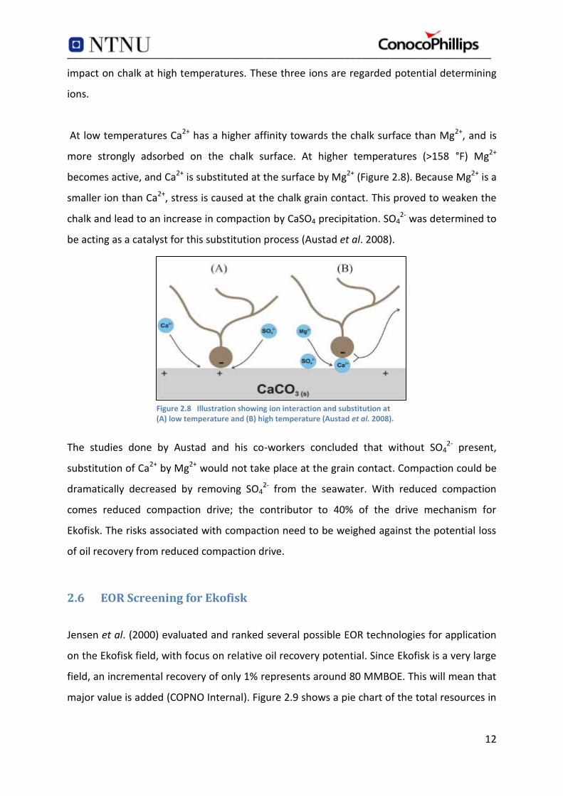
Figure 2.8 Illustration showing ion interaction and substitution at (A) low temperature and (B) high temperature (Austad et al. 2008).
impact on chalk at high temperatures. These three ions are regarded potential determining
ions.
At low temperatures Ca2+ has a higher affinity towards the chalk surface than Mg2+, and is
more strongly adsorbed on the chalk surface. At higher temperatures (>158 °F) Mg2+
becomes active, and Ca2+ is substituted at the surface by Mg2+ (Figure 2.8). Because Mg2+ is a
smaller ion than Ca2+, stress is caused at the chalk grain contact. This proved to weaken the
chalk and lead to an increase in compaction by CaSO4 precipitation. SO42- was determined to
be acting as a catalyst for this substitution process (Austad et al. 2008).
The studies done by Austad and his co-workers concluded that without SO42- present,
substitution of Ca2+ by Mg2+ would not take place at the grain contact. Compaction could be
dramatically decreased by removing SO42- from the seawater. With reduced compaction
comes reduced compaction drive; the contributor to 40% of the drive mechanism for
Ekofisk. The risks associated with compaction need to be weighed against the potential loss
of oil recovery from reduced compaction drive.
2.6 EOR Screening for Ekofisk
Jensen et al. (2000) evaluated and ranked several possible EOR technologies for application
on the Ekofisk field, with focus on relative oil recovery potential. Since Ekofisk is a very large
field, an incremental recovery of only 1% represents around 80 MMBOE. This will mean that
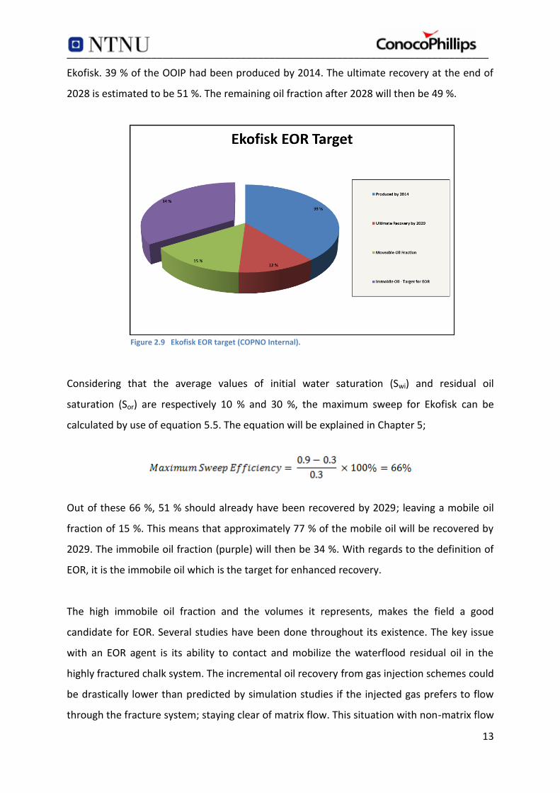
major value is added (COPNO Internal). Figure 2.9 shows a pie chart of the total resources in
___________________________________________________________________________
13
Figure 2.9 Ekofisk EOR target (COPNO Internal).
Ekofisk. 39 % of the OOIP had been produced by 2014. The ultimate recovery at the end of
2028 is estimated to be 51 %. The remaining oil fraction after 2028 will then be 49 %.
Considering that the average values of initial water saturation (Swi) and residual oil
saturation (Sor) are respectively 10 % and 30 %, the maximum sweep for Ekofisk can be
calculated by use of equation 5.5. The equation will be explained in Chapter 5;
Out of these 66 %, 51 % should already have been recovered by 2029; leaving a mobile oil
fraction of 15 %. This means that approximately 77 % of the mobile oil will be recovered by
2029. The immobile oil fraction (purple) will then be 34 %. With regards to the definition of
EOR, it is the immobile oil which is the target for enhanced recovery.
The high immobile oil fraction and the volumes it represents, makes the field a good
candidate for EOR. Several studies have been done throughout its existence. The key issue
with an EOR agent is its ability to contact and mobilize the waterflood residual oil in the
highly fractured chalk system. The incremental oil recovery from gas injection schemes could
be drastically lower than predicted by simulation studies if the injected gas prefers to flow
through the fracture system; staying clear of matrix flow. This situation with non-matrix flow

___________________________________________________________________________
14
could occur if matrix flow is prohibited by capillary threshold entry pressures or rate-limited
by gas-water diffusion (Jensen et al. 2000).
Figure 2.10 shows the waterflood and EOR investigation that has been going on for the
Ekofisk field since 1973.
Since 1975 swing gas has been re-injected into the crestal areas of the field. As of June 2000,
21% (1.3 Tscf) of the cumulative produced gas had been re-injected. Tracer tests done from
1986 to 1988 proved that the gas covered a large area, and that no immediate production of
free gas was experienced. In the late 1980s a nitrogen study was conducted, showing non-
favorable economics. The nitrogen only extracted the lightest components from the oil;
leaving the remaining oil less mobile, with higher viscosity and IFT.
The investigation into the possibility of implementing a WAG pilot was initiated in 1993. The
studies of injecting hydrocarbon gas alternate water showed promising results, and a pilot
test was planned. The pilot was executed in 1996, but was found to be both technically and
economically challenging. The many years of injecting cold seawater had created a cold
region around the injecting wells. This cold region caused the formation of hydrates in-situ in
Figure 2.10 Historical EOR studies and waterflood for Ekofisk (COPNO Internal).

___________________________________________________________________________
15
the reservoir, and injectivity dropped to zero in a matter of hours. Following the pilot,
studies were done to find ways in which hydrate formation could be avoided, but no real
solutions were discovered (Jensen et al. 2000).
In addition to the HC-WAG pilot and the waterflood pilot in the early 1980s, two other pilots
have been performed on Ekofisk. This was a water-shut-off pilot and a produced water pilot;
where neither of which has been published with results in the literature.
After the failed pilot test, a number of other EOR techniques were studied; air injection, CO2
WAG injection, smart water and surfactants. Air injection to create spontaneous ignition
around the cooled water injectors was studied between 2001 and 2006. The incremental oil
recovery from air injection proved to be the highest of the methods in the screening study
done by Jensen and his co-workers. Air injection was at the end ruled out due to the large
risk and uncertainty involved. Producing large amounts of oxygen together with oil and gas
creates a potential explosion hazard.
CO2 is not a likely option today due to the lack of CO2 availability and the potential need for
extensive field re-development. Some of the equipment on Ekofisk dates back to the start of
the field’s life, which would make corrosion a huge problem. The large amount of fractures
in the field also present problems for a possible CO2 flood, because it could lead to early
breakthrough of CO2. With the temperature profile created by injecting cold seawater, there
is also a potential risk of hydrate formation. This will cause injectivity losses similar to those
experienced in the WAG pilot. The subsidence increases the potential for well failure, which
increases the risk of leakage. There is also a high potential for CO2 leakage due to the fact
that more than 400 wells have been drilled during the last 40 years of production. A safe
aquifer would be needed for containment assurance. As of today, CO2 flooding is looked at
as a possibility for the future. A multi-well pilot would need to be carried out before a full
field implementation. Smart Water has been studied over the last couple of years, but is
currently not at a level where it is possible to quantify the EOR effect.
In the mid- to late 1990s an enhanced imbibition study by injection of low concentration
surfactants was conducted. The study was terminated in 1997 due to lab measurements of
unsatisfactory high adsorption, making it un-economical. The high adsorption was especially

___________________________________________________________________________
16
seen in the vicinity of existing water injection wells, where reservoir temperatures were
reduced. Further studies on surfactants were not done until 2011. Both the economics and
understanding of the surfactant process have improved significantly over the last 20 years,
making it an option once again.

___________________________________________________________________________
17
3 Theory
This chapter addresses the rock and fluid properties of particular interest for surfactant
flooding. This includes porosity, permeability, matrix-fracture interaction, interfacial tension,
wettability, relative permeability, saturation and spontaneous imbibition.
The two main parameters that determine the efficiency of surfactant flood as an EOR
technique are interfacial tension and wettability alteration. The two parameters play a
crucial part in the ability to recover what is left of the oil in the reservoir; reducing the
residual oil saturation.
3.1 Rock Properties
3.1.1 Porosity
Porosity is defined as the ratio of pore volume (void space) to the bulk volume of the rock
(Lake 1989);
Where φ is porosity, Vp the pore volume, and Vb the bulk volume. The porosity is normally in
the range of 10% to 40% (Lake 1989) for naturally occurring media; the rock phase clearly
occupying the largest fraction of any medium. For a rock containing all equally sized grains,
the grain size does not affect porosity. Grain size distribution and sorting however, play an
important role. Well sorted grains produce a much higher porosity than does poorly sorted
grains. Porosity can be divided into primary and secondary porosity. Basically, primary
porosity is formed when the sediments are first deposited, while secondary porosity is
formed by geological processes that take place after deposition (e.g. digenesis). The porosity
of sandstone is normally primary, while limestone typically has secondary porosity.
Furthermore, porosity can be divided into interconnected (effective) porosity and
disconnected porosity. The latter is of no concern to EOR, as the oil in disconnected pores
cannot be contacted by any displacing agent (Zolotukhin & Ursin 2000).
(3.1)

___________________________________________________________________________
18
Porosity is as high as 48 % in some parts of the Ekofisk formation. The high porosity can be
explained by the early invasion of oil into the reservoir rock; preventing the porosity from
being lowered by digenesis.
3.1.2 Permeability
Permeability is as important to EOR processes as porosity, and is defined as a medium`s
capability to transmit fluids through its network of interconnected pores (Zolotukhin & Ursin
2000). From this we can draw out that a medium can be porous yet not permeable, if there
are no interconnected pores across the whole medium for fluid to flow through. On the
other hand, a medium cannot be permeable without being porous. Permeability is usually
calculated by using Darcy`s equation for fluid flow through porous medium;
Where k is permeability measured in units of darcies (D) or millidarcies (mD), q is flow rate, μ
is viscosity, A is surface area and (ΔP/Δx) is the pressure gradient. In most reservoir rock,
primarily sandstone, there is a strong correlation between porosity and permeability. This
correlation is often used to determine permeability, as it is more difficult to measure than
porosity. It should also be noted that permeability is much more uncertain than porosity.
While porosity only varies a few percent spatially in a typical formation, permeability can
vary by three or more factors of 10 (Lake 1989).
The permeability of the Ekofisk formation, and chalk reservoirs in general, can be divided
into two categories; matrix permeability and fracture permeability. Typical matrix
permeability for Ekofisk is in the range of 0.02 – 10 md, with 5 md as the average. Faults or
fractures in chalk are not associated with flow barriers as they are in sandstone. Fracture
permeability is substantially higher than matrix permeability, and effective permeability is in
the range of 1 md to 100 md (COPNO Internal).
(3.2)

___________________________________________________________________________
19
Figure 3.1 Idealized matrix-fracture system (Warren & Root 1963).
3.1.1.1 Matrix-fracture Interaction (Single vs. Dual Porosity Model)
The dual porosity model involves both porosity and permeability. Naturally fractured
reservoirs typically have two distinct porosities; primary in the matrix and secondary in the
fractures. These two different porosities can be represented by corresponding
homogeneous porosity systems. The matrix contributes significantly to the storage capacity
of hydrocarbons, but has negligible contribution to the flow capacity. The concept of dual
porosity was developed based on the need to model the behavior of such matrix regions,
and distinguish them from fractures (Warren & Root 1963). The fractures provide an easy
path for fluid flow, but have limited hydrocarbon storage capacity. Figure 3.1 shows an
idealized representation of a matrix-fracture system. There are two distinct fluid flow types.
The first is the flow from the matrix to the fractures, and then to the wellbore. The other is
the direct fluid flow from the fractures to the wellbore.
Although a dual porosity model gives a more accurate representation than a single porosity
model, limitations with regard to computational resources make it impractical for full field
simulation problems. For this reason, a single-porosity model is used for the Ekofisk model.
By aligning the grid with the major fractures and adjusting the transmissibility between the
grid cells in the fracture, an approach to the real situation is achieved.

___________________________________________________________________________
20
Figure 3.2 Capillary equilibrium of a spherical cap (Tiab & Donaldson 2012).
3.2 Fluid-Rock Interaction
3.2.1 Interfacial Tension
Interfacial tension (IFT) exists when two immiscible fluids are in contact with each other. A
clearly defined interface, only a few molecular diameters thick, arises between the two
fluids. This happens because the attractive forces between the molecules internally in one
phase are larger than the attraction to the molecules in the other phase. This means that the
molecules on the surface of a drop will experience a net inward attraction. This attraction
ensures that the surface area of the drop is made as small as possible.
The definition of the IFT between two fluids, σ, is the force per unit length (newtons/meter),
and is often expressed as dynes/centimeter. This is numerically equal to millinewtons per
meter (mN/m). IFT is a measure of miscibility; the lower the IFT, the closer the two phases
are to being miscible (Tiab & Donaldson 2012). The action of the IFT is to reduce the size of
the sphere unless it is opposed by a great enough pressure difference (P2 – P1). Figure 3.2
shows the forces acting on a spherical cap.
The mechanical equilibrium of the interface is governed by the Laplace equation;
Where P1 is the external pressure acting on the spherical cap, P2 is the internal pressure,
(P2 – P1) is the capillary pressure (Pc), σ is the interfacial tension between the two phases,
and r1, r2 are the principal radii of the curvature.
(3.3)

___________________________________________________________________________
21
Figure 3.3 Wettability at solid-fluid interface. (a) Water-wet system (b) Neutrally-wet system (c) Oil-wet system (Tiab & Donaldson 2012).
3.2.2 Wettability
Wettability is the preferential affinity of the solid matrix for either the aqueous phase or the
oil phase. It is the tendency of a fluid to spread on or adhere to a solid surface in the
presence of other immiscible fluids (Elshahawi et al. 1999). Wettability determines the fluid
distribution in a porous medium, and is important for waterflood behavior as well as
enhanced recovery. Wettability controls the capillary pressure and relative permeability
behavior; hence also the rate of oil displacement and overall recovery.
The wettability of a reservoir rock can be quantified by the contact angle between the rock
surface and the fluid-fluid interphase; a value larger than 90° suggesting a water-wet system,
and a value less than 90° indicating an oil-wet system. For contact angle values close to 90°,
the system is referred to as mixed-wet or neutral. The contact angle, θ, is given by Equation
3.4;
Where σso is the IFT between the solid and oil, σsw is the IFT between the solid and water,
and σwo is the IFT between water and oil.
3.3 Relative Permeability
Relative permeability is a dimensionless term created to adapt Darcy equation to account for
multiphase flow conditions. If only one fluid is present in the rock, the relative permeability
(3.4)

___________________________________________________________________________
22
Figure 3.4 Typical water-oil relative permeability curves for (a) water-wet & (b) oil-wet system (Tiab & Donaldson 2012).
of this fluid will be 1. Relative permeability is defined as the ratio of the phase permeability
to the absolute permeability, and is a number between 0 and 1;
Where i is the phase, kri is the relative permeability of the phase, and k is the absolute
permeability. Calculating relative permeabilities allows for comparison between different
abilities of fluid to flow in presence of each other. The relative permeability to a phase
decreases as the saturation of the phase decreases. When kri approaches zero, the phase can
no longer flow. This corresponds to the critical phase saturation, Sci; defined as the lowest
level of saturation at which a phase is left immobile (Cinar 2013).
Endpoint relative permeability is also an important property, defined as the kr of a phase at
the other phase`s residual saturation. Endpoint kr is denoted by an o in superscript, and is a
measure of the rock wettability. The wetting phase`s kro will be smaller than the non-wetting
phase`s kro. Another good indication of wettability is the crossover point of a relative
permeability curve (where kr1 = kr2). (Lake 1989)
Figure 3.4 shows the relative permeability curves for strongly water-wet rock to the left, and
a strongly oil-wet rock to the right. For strongly water-wet rock the crossover point is larger
than Sw=50%, while it is smaller than Sw=50% for strongly oil-wet rock.
(3.5)

___________________________________________________________________________
23
3.3.1 Pseudo Relative Permeability Curves
A large number of grid cells are needed to simulate large field models. Pseudo relative
permeability curves are used to reduce the dimensionality of the models. They are also used
to account for intra-cell rock property variations. Pseudo relative permeability curves are
most affected by the dip angle of the reservoir, but are also highly dependent on layer
thickness and PVT properties (Saud & Abdulaziz 1998).
Pseudo relative permeability curves can be applied to two-dimensional reservoir simulator
models to approximate the three-dimensional solution. The pseudo curves account for
vertical heterogeneity, known as stratification. The properties needed to calculate the
pseudo relative permeability curves are permeability, thickness, porosity, connate water
saturation, residual oil saturation and the end point relative permeabilities of the different
layers in the model (Hearn 1971).
3.4 Saturation
The saturation, S, of a particular fluid phase i in a rock is the fraction Vi of the total pore
volume (PV) this fluid occupies;
It is believed that before the invasion of petroleum, the pores are completely filled with
water. As oil or gas migrates to take the waters place, it does not manage to replace all the
water. To determine the quantity of oil and gas, it is necessary to determine the different
saturations of water, oil and gas in the pore space. There are especially three important
saturation terms worth mentioning:
Swi is the initial water saturation in the reservoir. This is the mentioned water that is
not displaced as oil migrates upwards to fill the pores.
Swirr is the irreducible water saturation, and refers to the lowest water saturation that
can be achieved when displacing water with oil or gas.
(3.6)

___________________________________________________________________________
24
Sor is the residual oil saturation, and is defined as the oil which cannot move during
fluid flow in primary or secondary recovery. EOR methods aim to increase recovery
by reducing this value.
The total saturation of a rock should always add up to unity. For two-phase flow of oil and
water, the simple equation for saturation becomes;
For three-phase flow of oil, gas and water, the same equation becomes;
Where the saturations are Sw for water, So for oil and Sg for gas.
3.4.1 Spontaneous Imbibition
Imbibition is defined as the exchange between oil in the matrix and water in the fractures as
a result of capillary action. Imbibition can be divided into spontaneous and forced
displacement. Spontaneous imbibition is especially important for highly heterogeneous
reservoirs, such as fractured-matrix reservoirs. Water will be imbibed into the matrix from
Figure 3.5 Two-phase relative permeability curves; water-oil system – imbibition.
(3.8)
(3.7)

___________________________________________________________________________
25
fractures with a countercurrent flow of oil into the fractures. The oil is then free to flow
towards the production wells through the fracture network (Morrow & Mason 2001). If a
rock is oil-wet, water needs to be forced into the rock in order to displace oil. This process
corresponds to forced imbibition. The spontaneous and forced parts of a capillary imbibition
curve are indicated in Figure 3.6.
Figure 3.6 Spontaneous and forced imbibition and drainage capillary pressure curves (Morrow & Mason 2001).

___________________________________________________________________________
26

___________________________________________________________________________
27
4 Literature
Development of mature fields has become popular due to the decline in new field
discoveries and the currently high oil prices. Average recovery factors for carbonate
reservoirs are 30 % (Sheng 2013). Prior to the major increase in oil prices this oil was often
not economically viable to extract by applying EOR methods. However, with the change in
economics and the ever increasing demand for oil, the times have changed.
Chemical EOR is generally applied to fields that have undergone waterflooding over a long
period of time, and have significant water cuts. For reservoirs with low temperatures and
low salinity brines, EOR chemicals have been applied for over 80 years. The challenge lies in
developing chemicals for high temperature and high salinity reservoirs. The majority of
production comes from exactly reservoirs with high temperature and high salinity;
representing a vast potential for chemical EOR. Oil production from EOR is today less than
5% worldwide (Siggel et al. 2012). Most of these 5 % come from thermal methods or use of
miscible gas rather than chemical flooding.
Two issues are critical in the development of mature fields: determining the main reasons
for the low production or high ROS, and finding the optimum economical solution with
minimal risk.
4.1 Surfactant Flooding
Surfactants are surface active agents, meaning that they act on the rock surface. In a
surfactant flood the aim is to alter the rock wettability and/or lower the interfacial tension
(IFT) between water and oil to recover the capillary-trapped oil after waterflooding. These
capillary trapped oil droplets can constitute more than half of the residual oil. An efficient
surfactant can reduce IFT by a factor of 104 (Zolotukhin & Ursin 2000).
Some challenges related to field application of surfactants is finding a suitable surfactant for
specific reservoir conditions. The surfactant needs to demonstrate optimal phase behavior
at reservoir conditions. The most challenging properties to handle are reservoir pressure,

___________________________________________________________________________
28
reservoir temperature and brine salinity. Other factors for a surfactant flood to be successful
are low cost of the chemical, manageable logistics, good injectivity and low adsorption.
Optimizing a surfactant flood is a compromise between achieving ultralow IFT, low retention
and sufficient injectivity (Sheng 2013).
Surfactants are often used in combination with alkali and polymer to form an alkaline-
surfactant-polymer (ASP) flood. Figure 4.1 illustrates the sequence of an ASP flood.
The target reservoir is usually first flooded with a preflush bank of water to flush the
formation brine out of the reservoir. This can reduce the amount of chemicals needed and
create optimum conditions for the surfactant flood. The ASP slug is then injected to mobilize
the trapped oil and reduce the residual saturation; creating a new oil bank. The volume
chemicals required is typically between 15 % and 30 % of the pore volume (Ahmed &
Meehan 2012). This slug is followed by a polymer slug which aims to provide mobility
control; improving the sweep efficiency. Without this mobility buffer there is a risk of water
fingering through the ASP slug; diluting and dispersing the slug. If the concentration of the
chemical slug falls below a certain value, it will no longer work as designed. Finally, chase
water is injected to drive the new oil bank towards the producer. Chase water is injected
until the economic limit of the project is reached (Ahmed & Meehan 2012). The economic
limit is typically a specified water cut or oil rate.
Figure 4.1 Representation of an ASP flooding sequence (COPNO Internal).

___________________________________________________________________________
29
4.1.1 Types of Surfactants
A typical surfactant monomer consists of a nonpolar portion and a polar portion, making it
attracted to both water and oil. The nonpolar portion has a strong affinity for oil, and the
polar portion a strong affinity for water; giving the surfactant a distinct dual nature. It is
because of this dual nature it has the ability to alter rock wettability. A surfactant monomer
is often represented by a tadpole symbol, with the polar part being the head and the
nonpolar part being the tail. The nature of the polar portion classifies the surfactant as one
of four groups; anionic, cationic, nonionic or amphoteric (Lake 1987). The most widely used
surfactants for EOR purposes are cationic and anionic. Cationic surfactants have a positively
charged head group, while it is negatively charged for anionic surfactants (Figure 3.2).
Nonionic surfactants mainly serve as cosurfactants to improve system phase behavior
(Sheng 2011).
Cationic surfactants are efficient in altering wettability from oil-wet to mixed-wet or water-
wet. By means of electrostatic forces they interact with anionic crude oil compounds
adsorbed on the chalk. Cationic monomers form ion-pairs with the negatively charged
carboxylates of crude oil; desorbing them from the chalk. Once the adsorbed material is
released from the surface, the chalk becomes more water-wet. This process of wettability
alteration is irreversible, as the ion-pairs are only soluble in the oil-phase (Sheng 2013).
Anionic surfactants do not desorb the negative oil compounds in the same irreversible
manner as the cationic surfactants. However, they can create a surfactant double-layer
between the oil and the chalk, which has demonstrated to slowly displace oil spontaneously
(Sheng 2013). Because the bonds of the double-layer are weak it is not regarded a
Figure 4.2 Representation of (a) cationic surfactant and (b) anionic surfactant.

___________________________________________________________________________
30
permanent wettability alteration. The main goal of anionic surfactants is reducing the IFT.
Anionic surfactants are often combined with nonionic surfactants to increase their tolerance
to salinity (Sheng 2011).
Several surfactant formulations have been developed for Ekofisk conditions in the
Bartlesville laboratory. The current formulations are anionic surfactants with sulphonate
groups (COPNO Internal).
4.1.2 Microemulsion Phase Behavior
Winsor (1954) classified surfactant/oil/water microemulsions as Type I (oil in water), Type II
(water in oil) or Type III (bicontinuous oil and water in a third phase known as the middle
phase microemulsion). Type III exhibits the lowest IFT, and is related to the term optimum
salinity developed by Healy & Reed (1974). They showed how phase volumes in
microemulsion systems could be correlated with IFT`s and oil recovery. The goal since then
has been to maximize oil recovery under these optimum conditions, and to maintain them as
long as the surfactant flows through the reservoir (Robertson 1988).
A microemulsion is defined by Healy & Reed (1974) as “a stable, translucent micellar-
solution of oil and water that may contain electrolytes, and one or more amphiphilic
compounds” (surfactants, alcohols, etc.). According to this definition a microemulsion
distinguishes itself from an emulsion by not necessarily having a distinct external phase. A
microemulsion has at least three components – oil, water and surfactant – which can be
represented by a ternary diagram, as showed in Figure 4.3. Differences among the various
microemulsions and surfactant flooding processes simply reduce to variations in location of
injection composition on the ternary diagram.

___________________________________________________________________________
31
Figure 4.3 Ternary diagram of microemulsion system (Healy & Reed 1974).
As long as the composition of the microemulsion slug allows it to stay in the single-phase
region, displacement will be miscible, and all of the oil is recovered. Once the composition
enters the multi-phase region, displacement of the slug will be immiscible. Two important
criteria for a microemulsion to effectively recover oil were made clear by Healy; the
multiphase region should be minimal to prolong miscible displacement in the single-phase
region, and the IFT in the multiphase region should be low to enhance immiscible
displacement.
There are at least two reasons for considering IFT in regards to microemulsion systems. One
is that whenever IFT is measured between water and oil in the presence of surfactant, there
is a large possibility that one or both phases are microemulsions. The second reason is that
once a microemulsion bank enters the multiphase region, oil recovery is driven by low IFT
immiscible displacement. Furthermore, IFT depends on both salinity and cosurfactant
concentration, and can vary almost three orders of magnitude within a given multiphase
region. Salinity determines the IFT distribution, and affects the size, shape and connectivity
of the multiphase region (Healy & Reed 1974).

___________________________________________________________________________
32
4.1.3 Optimum Salinity for Ultralow IFT
Surfactant flooding in combination with low salinity water has revealed a boosting effect on
enhanced oil recovery in recent research. There are three main advantages of the low
salinity environment; it may reduce re-trapping of mobilized oil, reduce
adsorption/retention and make more low cost surfactants available for use (Skauge 2013).
The purpose of reducing IFT to ultralow values is to mobilize the disconnected oil droplets
typically left behind after a waterflood; considered residual oil. Ultralow IFT generally only
exists in a narrow salinity range near the optimum salinity. To achieve this, the approach
suggested for Ekofisk is one where a salinity gradient is applied. The active region containing
the surfactant is flanked by overoptimum salinity ahead, and underoptimum salinity behind.
This way, the salinity profile is certain to pass through the optimal salinity somewhere in the
displacement front region (Hirasaki et al. 2011). Figure 4.4 shows a visual representation of
the salinity gradient. The x-axis represents the distance from injector to producer, and is
plotted against salinity on the y-axis.
The salinity gradient works in the following manner:
1. The system is overoptimum ahead of the active region. This retards the surfactant
by partitioning into the oil phase.
Figure 4.4 Salinity gradient (COPNO Internal).

___________________________________________________________________________
33
2. The residual oil displacement takes place as the system passes through the active
region of ultralow IFT (Winsor III).
3. The system is underoptimum behind the active region. Lower-phase
microemulsion takes place, and the surfactant propagates with water velocity.
The surfactant slug is in practice injected in a near- to underoptimum salinity environment.
By applying this practice, the gradient ensures that if overoptimum conditions are for some
reason reached during the process, the lower salinity behind the surfactant slug will still
allow optimal conditions to be achieved; releasing surfactant trapped in the oil.
Optimum salinity is a function of surfactant concentration and water oil ratio (WOR) for an
alkaline/surfactant system. It is also dependent on the soap/surfactant ratio, unless the soap
content is negligible or the soap and surfactant have the same optimum salinity. The
soap/surfactant gradient exists because the soap is generated in-situ, while the surfactant is
introduced with the injected fluid (Hirasaki et al. 2011).
4.1.4 Surfactant Retention
The propagation of surfactant through the reservoir is limited by its retention. Surfactant
retention includes phase trapping, unfavorable phase behavior and adsorption. It is an
important factor to consider because it leads to loss of surfactant as the slug moves through
the reservoir. The economic viability of a surfactant flood is highly dependent on the volume
chemicals required in the process. It should also be noted that if the surfactant slug is highly
dispersed it may no longer work as designed. If the concentration of surfactant falls below a
critical value, it will no longer form microemulsions and obtain the desirable effects
associated with the Type III behavior. Grigg & Mikhalin (2007) claimed that surfactant loss
through partitioning into the oil phase and through adsorption onto the rock surface often
consumes more than 90 % of the surfactant in the system. The partitioning of surfactant into
crude oil can be responsible for as much as 30 % of the losses, while adsorption is
responsible for the major part of retention. Retention varies widely depending on surfactant

___________________________________________________________________________
34
structure, mineralogy, brine salinity and hardness, wettability, pH, microemulsion viscosity,
temperature, crude oil, co-solvent and mobility control among others (Solairaj et al. 2012).
The research done by Solairaj and his co-workers concluded that surfactant retention would
be low for an optimized surfactant formulation with good mobility control and a favorable
salinity gradient. They further stated that retention decreases with increasing pH, acid
number, temperature or oil reactivity.
Adsorption of surfactant on solid surfaces can modify surface hydrophobicity, charge and
other key parameters important for the interfacial processes in enhanced oil recovery. The
forces generally controlling adsorption are covalent bonding, electrostatic attraction,
hydrogen bonding, solvation and desolvation. Which forces that dominate a surfactant-solid
system depends on the solid and surfactant type, surfactant concentration, electrolyte, pH,
temperature etc. Adsorption of anionic surfactant is for instance higher on a positively
charged surface than on a negatively charged surface, while cationic surfactants adsorb
more on negatively charges surfaces (Zhang & Somasundaran 2006). This is due to the fact
that anionic surfactants have a negatively charged head group, while it is positively charged
for cationic surfactants.
4.2 Recent Advances in Surfactant EOR
Of the petroleum present in known reservoirs, it is currently considered that about one third
of it is economically recoverable. Improving recovery by use of surfactants was an idea
already in 1927, but early results were not encouraging, and the process mechanisms were
not understood. In the 1960s the interest in surfactant EOR was revitalized through miscible
flooding research, and the results were more promising. It was however not initially
recognized that process success also depended on maintaining ultralow IFT at the rear of the
slug, where it was displaced by an aqueous polymer solution and became a Winsor 1
microemulsion (Hirasaki et al. 2011). As described by Winsor (1954) there are three phases
of microemulsion behavior; lower-phase (I), upper-phase (II) and middle-phase (III).

___________________________________________________________________________
35
Surfactants work in means of wettability alteration and/or producing ultralow IFT. By
altering the wettability, imbibition is increased. Achieving ultralow IFT by lowering the
capillary number makes it possible to displace oil from preferentially oil-wet carbonate
matrix to fractures by oil/water gravity drainage. The process depends on the surfactant
forming microemulsions in the oil and water phases to be able to free the trapped oil. Work
by Pennel et al. (1996) revealed that at typical reservoir velocities, IFT between crude oil and
brine had to be reduced from values of 20 to 30 mN/m to values in the range of 0.001 to 0.1
mN/m to achieve low residual oil saturation values (<0.05) (Hirasaki et al. 2011). In the 1970s
systematic variations of IFT when changing variables as salinity, oil composition and
temperature were found.
As salinity increased, it was discovered that the surfactant was able to solubilize an
increasing amount of oil and decreasing amount of water. The point where the surfactant
microemulsion solubilized equal amounts of oil and water was called the optimum salinity.
The appearance of a middle-phase microemulsion depends on the amounts of water, oil and
surfactant present (Hirasaki et al. 2011). In order to have a successful displacement process,
the injected surfactant slug must first achieve ultralow IFT to mobilize residual oil and create
an oil bank. The oil and water should both flow as continuous phases. Secondly, to prevent
mobilized oil from being re-trapped by capillary forces, ultralow IFT must be maintained at
the displacement front.
Prior to the work of Abe et al. (1986) it was thought that alcohol was necessary as a
cosolvent to have a microemulsion with an anionic surfactant. It was later proved that by
using a branched surfactant, microemulsion without a cosolvent was possible at room
temperature. Although it is not necessary, the use of a cosolvent can alter the optimal
salinity required to achieve ultralow IFT. A disadvantage of using alcohol is that it decreases
solubilization of oil and water in microemulsions; increasing the minimum obtainable value
of IFT with a given surfactant.
The long-term stability of a surfactant at reservoir conditions is a requirement for any
surfactant. Surfactant hydrolysis is limited up to temperatures of 50-60 °C at slightly alkaline

___________________________________________________________________________
36
pH levels and a modest concentration of calcium (Hirasaki et al. 2011). For reservoirs at
higher temperatures, surfactants with other head groups will be needed.
The process of combining surfactants with alkali to optimize surfactant effect was presented
by Nelson et al. (1984). The role of the alkali is to reduce surfactant adsorption as the slug
propagates through the reservoir. Also, alkali generates soap in situ; allowing the surfactant
to be injected at lower salinities, which further reduces the adsorption of the chemical. This
allows for a smaller volume of surfactant to be used. However, adsorption is only one
component of surfactant retention. A more significant process can be found in the phase
trapping of surfactants. In order to have an effective process in a fractured oil-wet reservoir,
the combined effect of surfactant and alkali in shifting matrix wettability towards water-wet
is of the essence.
Formation wettability can be altered by pH, surfactants that adsorb on the minerals or
remove adsorbed naphthenic acids, and acids or bases. Since carbonate formations are likely
to be fractured, they will depend on spontaneous imbibition or buoyancy for displacement
of oil from the matrix to fractures. Spontaneous imbibition is the process where the wetting
fluid is drawn into a porous medium by capillary action. When low IFT is achieved with a
surfactant, capillary pressure is reduced to negligible values; eliminating the process of
spontaneous imbibition. Under these conditions, gravity becomes an important contributor.
For a given system, temperature is an important factor for wettability alteration and rate of
imbibition oil recovery (Hirasaki et al. 2011).
4.3 Environmental Regulations of EOR Chemicals
Offshore installations create major challenges related to the handling and discharge of back-
produced water containing EOR chemicals. Use of chemicals in the Norwegian sector of the
North Sea is subjected to restrictions by the Norwegian Environmental Regulations. Use and
discharge of EOR chemicals needs to be approved by Klif (Climate and Pollution Directorate).
The chemicals are classified into four groups based on their level of ecotoxicity. The groups
are green, yellow, red and black; black being the most toxic, least biodegradable and with
the highest risk of bioaccumulation. Both the red and black chemicals are harmful, and
should only be chosen if they are necessary for technical and safety reasons. There is a zero

___________________________________________________________________________
37
Figure 4.5 Discharge of red and black chemicals on the NCS (Miljødirektoratet 2013).
discharge policy for red and black chemicals on the Norwegian sector. As seen from Figure
4.5, the use of these chemicals has decreased to a very low level the last couple of years. In
2012 the total discharge was 10.4 tons.
Extensive implementation of chemical EOR techniques on the NCS will lead to a large
increase in the usage of toxic chemicals. Still, it must not be forgotten that a 1% increase in
production of the proven resources on Norwegian fields equals a gross value of 270 billion
NOK (FORCE report 2011). The economic impact of implementing EOR techniques can be
remarkable both for operator, licenses and the Norwegian society.
The environmental challenges are related to the handling of chemicals during chemicals
preparation, injection, back production and discharge to sea. The zero discharge policy is not
necessarily a show stopper for the use of red and black chemicals for EOR purposes. The
chemical bearing produced water can be re-injected, or the chemicals can be separated from
the water. Looking at it from a holistic perspective, EOR techniques often reduce water cuts,
which can lead to reduced CO2 emission.

___________________________________________________________________________
38

___________________________________________________________________________
39
5 Factors Influencing Recovery
A number of factors influence the overall recovery of a reservoir. Horikx et al. (2013)
presented twelve factors most important for oil recovery in chalk oil fields, and also
subdivided them;
Lateral Reservoir Qualities:
o Faulting & macro-fracturing
o Lateral permeability variation
Vertical Reservoir Qualities:
o Net to gross
o Vertical connectivity
o Vertical permeability profile
Dynamic Aspects:
o Moveable oil fraction
o Wettability
o Compaction drive potential
o Gas cap & bubble point
o Oil Mobility
Geography & Economics:
o Location of field
o Effective oil column
The more general displacement mechanisms are presented in the subchapters below.
5.1 Displacement efficiency and Volumetric sweep efficiency
Displacement efficiency (ED) and volumetric sweep efficiency (EV) are equally important to
the total recovery of oil. ED is a function of time, fluid viscosities, relative permeabilities and
capillary pressure. EV is a function of time, viscosities, well arrangements, heterogeneity,
gravity and capillary forces. All efficiencies are numbers between 0 and 1 (Lake 1989).

___________________________________________________________________________
40
Displacement efficiency is defined as the ratio of oil displace to the amount of oil contacted
by the displacing agent, assuming constant oil density;
Where Soi is the initial oil saturation, So,avg is the average oil saturation of the swept zone and
Sor is the residual oil saturation in the swept zone. A higher ED will be achieved by reducing
So,avg.
Volumetric sweep refers to the reservoir`s volume that can be invaded by a displacing agent.
Volumetric sweep is the product of areal and vertical sweep efficiency; respectively EA and EI;
EA and EI both depend on each other, and a large mobility ratio is detrimental to both
efficiencies. Areal sweep (Equation 5.3) refers to the horizontal area that can be swept,
while vertical sweep (Equation 5.4) refers to the cross-sectional area that can be invaded;
EA is normally determined from displacement in scaled physical models. It depends on well
pattern, and increases as the flow pattern approaches linear flow. It also increases with
increased injection time and decreasing mobility ratio. Other factors determining areal
sweep are fluid mobilities, areal heterogeneities and the total injection volume (Ahmed &
Meehan 2012). EI is a measure of the flood`s effectiveness in overcoming heterogeneities in
the vertical direction, and is controlled by gravity-, capillary- and viscous forces in varying
degree (Cinar 2013).
(5.1)
(5.2)
(5.3)
(5.4)

___________________________________________________________________________
41
Furthermore, the volumetric sweep efficiency is defined as the ratio of oil contacted to the
amount of oil initially in place. It can also be defined as the moveable oil fraction;
5.2 Recovery Factor
Recovery factor ER is the product of displacement efficiency ED and volumetric sweep
efficiency EV;
Taking typical values of connate water and residual oil saturations should give an ultimate
displacement efficiency of 50% - 80% of contacted oil in a waterflood. Based on empirical
equations and figures, the volumetric sweep should be around 40% - 60% for a waterflood
(Lake 1989). This would give a resulting recovery factor between 16% and 48%; meaning that
over half of the original oil in place could be left in the ground after an even so successful
waterflood.
(5.5)
(5.6)

___________________________________________________________________________
42

___________________________________________________________________________
43
6 The EOR Process in General
EOR is oil recovery by means of injecting materials not normally present in the reservoir. This
definition does not restrict EOR to a particular phase, as it can be implemented at any stage
of the reservoirs life. There are three main stages of recovery. Primary recovery is defined as
recovery by natural drive mechanisms; e.g. water drive (aquifer influx), gas cap drive,
solution gas or gravity assisted drainage. Secondary recovery is mechanisms that aim to
maintain reservoir pressure, such as gas- or water injection. Any technique applied after
secondary recovery is referred to as tertiary recovery (Lake 1989).
Polymer flooding is not considered an EOR technique in accordance with the definition of
EOR in this thesis. The aim with polymer flooding is improving the sweep efficiency; not to
reduce the residual oil saturation. Polymer flooding falls into the category of IOR. It is all the
same included in this chapter as it is more often than not referred to as an EOR technique.
Waterflooding as a secondary recovery method has become very common, and is the most
frequently applied recovery technique in North Sea reservoirs. Injecting water helps both to
maintain reservoir pressure and increase recovery over natural driving forces, but still yields
low sweep efficiency and a poor production performance in most reservoirs. This is mainly
due to the impact of reservoir heterogeneities, problems related to well siting and spacing,
as well as the unfavorable mobility ratio between the displacing fluids (water, gas) and
displaced fluids (oil). Channeling of water or gas through more permeable flow paths causes
early breakthrough of the injectant as well as high water cuts.
EOR methods can be classified into three main categories; thermal, solvent and chemical
methods. Thermal methods include steam drive, steam soak and in-situ combustion. Solvent
methods refer to injection of natural gas, CO2, air, nitrogen or flue gas, among others, with
the aim to extract incremental oil by changing the phase behavior of the crude oil. The last
category of chemical methods involves flooding the reservoir with polymer, micellar
polymer, surfactants, foam or alkaline (high-pH) chemicals. In recent years several of these
methods have been combined in attempt to gain an even more efficient incremental

___________________________________________________________________________
44
Figure 6.1 Oil resources and reserves for the 25 largest Norwegian oil fields (NPD).
recovery (e.g. Alkaline-surfactant-polymer flooding). Smart Water and Low Salinity flooding
also fall into the category of chemical EOR because the water used is chemically altered.
Oil volumes can be divided into resources and reserves. Resources are an estimate of the
amounts of oil and gas that are believed to be physically contained in discovered and
undiscovered accumulations. Reserves are defined as the part of the resources which is
commercially recoverable in known reservoirs; given present economics and technology. As
oil and gas prices change, or new technology is presented, present reserves may be added or
deducted;
The four methods of adding to reserves are (1) Discovering new fields, (2) Discovering new
reservoirs, (3) Extending reservoirs in known fields, and (4) Redefining reserves because of
change in economics and/or extraction technology. EOR clearly falls into the two last
categories. Since the discovery of new fields and reservoirs is limited, the need for additions
by means of EOR is clear. Figure 6.1 shows the remaining oil resources and reserves in
Norwegian fields at the end of 2013. The remaining in-place resources make up half or more
of the total resources in most of the fields. This creates a vast potential for EOR processes.
Only Statfjord has produced more oil than Ekofisk by the start of 2014. The figure clearly
shows that Ekofisk has the largest quantities of both remaining reserves and resources.
(6.1)

___________________________________________________________________________
45
Incremental oil is the increased oil recovery by implementing EOR processes compared to
the recovery from doing nothing or from continued waterflood. Incremental oil recovered is
the measure of the success of any EOR project.
The goal with implementing EOR is often to mobilize more oil than is possible with only
water flooding/ primary production, and reducing the residual oil saturation. This is achieved
by increasing the volumetric and displacement sweep efficiencies. Different types of EOR
processes achieve this in different ways. Techniques involving thermal recovery methods
aim to reduce the oil viscosity to make it flow more easily. Polymer flooding gives a more
favorable mobility ratio, reducing viscous fingering and thereby increasing sweep efficiency.
Alkaline flooding aims to reduce the effect of capillary forces and alter the rock wettability,
and is often used in combination with surfactants. A surfactant flood aims to alter the rock
wettability and/or change the interfacial tension (IFT) between water and oil; freeing more
oil to flow.
In order for an EOR fluid to have the desired effect, it needs to get in contact with the
trapped oil. This has proved to be a special problem in naturally fractured reservoirs. The
main volume of oil is located inside the matrix, which is separated from the fracture
network. Because of this, there is major difficulty in getting EOR fluids to contact and
displace oil. There is no real way to assure matrix flow in an EOR process (Miller 2010).

___________________________________________________________________________
46

___________________________________________________________________________
47
7 EOR Methods with Basis in Waterflooding
Most chemical EOR techniques have their basis in water flooding. Not only is water a good
means of transporting chemicals, it is also good for dissolving them. These EOR techniques
can be implemented either before or after a field is flooded with water. Adding chemicals to
water can slow down water breakthrough and reduce water cut significantly, making a
project economically viable for a longer period of time; thereby extending field life.
7.1 The Screening Criteria
Not every reservoir will be adequate for implementing EOR methods. Both geological and
geographical conditions need to be analyzed under varying reservoir conditions to
determine the applicability of EOR methods. Table 7.1 features a list of screening criteria
retrieved from a paper by Taber et al. (1997).
Table 7.1 The screening criteria (Taber et al. 1997).
Each reservoir will have to be screened to see if it matches the requirements for one or
several methods. A project will require a choice of injection fluid and an overall process to
maximize the incremental oil, while still making a profit. With this said, a reservoir may fit

___________________________________________________________________________
48
the screening criteria for several different EOR methods, and it is up to the engineers to
choose the best one for their exact purpose of the project. The best option will depend on
several factors: oil price, injection fluid price, cost of chemicals, environmental regulations,
available facilities and so on. The screening criteria are based on field experience, and are
not set in stone. New technology and successful pilots or projects can require the screening
criteria to be reevaluated and changed.
7.2 Chemical EOR Methods
7.2.1 Polymer Flooding
A big issue with water flooding is the amount and extent of viscous fingering, and the poor
sweep efficiency that is achieved. Polymer flooding is an IOR technique that aims to increase
the viscosity of water. By adding polymer to the injection water, water viscosity increases,
and the mobility ratio becomes close to or even smaller than unity. The mobility ratio is
defined as the mobility of the displacing phase (water) over the mobility of the displaced
phase (oil);
As the mobility decreases, viscous fingering is reduced. The fingers become smaller and
more branched, resulting in a much larger area being swept at breakthrough. Less oil is
bypassed, and this results in increased areal-, vertical- and displacement sweep efficiencies;
leading to an overall higher recovery (Sheng 2012). Figure 7.1 shows a comparison of sweep
efficiency in water flooding and polymer flooding. The top three images display the
waterflood, while the bottom three images display the polymer flood. The sweep efficiency
is clearly higher for the polymer flood. Also, the breakthrough for the polymer flood occurs
at a much later time than for the water flood.
(7.1)

___________________________________________________________________________
49
7.2.2 Alkaline Flooding
Alkaline flooding is flooding the reservoir with high-pH chemicals with aim to reduce the
effect of capillary forces and alter the wettability. When an alkaline solution reacts with acid
in the crude oil, soap is generated in situ. The principal mechanism of alkaline flooding is
reducing the IFT between oil and water. Another mechanism is emulsification. Both the
formations of oil-in-water and water-in-oil emulsions can effectively improve oil recovery.
Alkaline solution is able to infiltrate the residual oil and created some discontinuous water
ganglia inside the oil phase to form water-in-oil emulsion. This causes an increase in the
resistance to flow in water fingers; diverting the injected water to unswept regions and
improving oil recovery. The formation and flow of these emulsions can result in significant
reduction in water-phase relative permeability (Surkalo 1990) and (Wang et.al 2010). Alkali is
often used in combination with surfactants to optimize the effect of the surfactant.
7.2.3 Low Salinity Waterflooding
Low salinity waterflooding (LSW) falls into the category of EOR because the water in this
process is altered in some way. LSW is the injection of water with lower salinity than the
initial formation brine salinity. By applying LSW, some chemically and physically processes
are provoked. Together these processes tend to enhance the recovery of oil in some
reservoirs. The amount of incremental oil produced is, however, very dependent on the
initial reservoir properties. EOR by LSW is a fairly new and unpredictable method. It has been
Figure 7.1 Comparison of sweep efficiency in water flooding (top) and polymer flooding (bottom) (Sheng 2012).

___________________________________________________________________________
50
successful for some pilot tests and projects, but the criteria for it being applicable are not
fully understood. Three conditions seem to be especially important for a LSW to be effective;
the presence of a significant clay fraction, connate water and the exposure of crude oil to
create mixed wettability conditions (Morrow & Buckley 2011). Initial wettability and end
point saturations also play an important role (Ashraf et al. 2010).
7.2.4 Smart Water
Smart Water is water with altered composition; not unlike the process of LSW. Smart Water
is made by modifying the ion composition of the water. Because this EOR method does not
require the use of chemicals, it is regarded environmental friendly. Smart Water can improve
wetting properties of oil reservoirs and optimize fluid flow and oil recovery. The concept is
developed by studying the chemical mechanisms happening during a waterflood. Addition of
sulfate ions (SO4-) in seawater has proved to have a positive effect on spontaneous
imbibition and total oil recovery in chalk. Two other ions are also active in this process; Mg2+
and Ca2+ (Austad 2013).
7.2.5 Microbial EOR
Microbial EOR (MEOR) is EOR by means of using resident microbes or introducing microbes
to the reservoir for the purpose of mobilizing trapped oil by reducing IFT, selectively plugging
of high permeability zones and reducing oil viscosity. The only essential difference between
MEOR and chemical EOR is in the method of introducing the recovery-enhancing chemicals
into the reservoir. Microbes produce chemicals in-situ in the reservoir by feeding on a
carbon source. Using residual oil as a carbon source would make the cost and logistics of
field implementation closer to that of a waterflood than to that of a chemical EOR process
(Bryant & Lockhart 2002).
Another technology involving microbes is microbial permeability profile modification
(MPPM). This method aims to restrict flow in watered-out channels, and forcing injection
water into unswept channels. MPPM technology differs from most MEOR methods by its
reliance on the in-situ micro flora rather than on injecting microbes into the reservoir
(Brown et.al. 2002).

___________________________________________________________________________
51
8 The Ekofisk Model
This chapter presents the Ekofisk simulation model. Included is a history match of the water
flooding sequence in the observation well (C11), a short introduction to PSim, a relative
permeability study and a 2D Ekofisk Sector model study.
8.1 History Matching
History matching is the act of changing a model to make it reproduce the past behavior of a
reservoir. By achieving this history match, the model can be used to predict future behavior
with a high degree of certainty. In this case the aim was to match the waterflooding
sequence of the different layers in a specific well located in the middle of the Ekofisk Field.
The reservoir pressure was also matched, but to a higher degree of uncertainty.
The observation well C11 was the main point of study in this part of the research. Water
breakthrough data from C11 was used to history match a 2D simulation model constructed
in PSim. Breakthrough times were matched by altering permeability and transmissibility in x-
and z-directions. Also, to get the spontaneous imbibition effect observed in the Lower
Ekofisk formation, capillary pressure data was added. A critical property to match was the
degree of dispersion of the displacement front. The observation suggested a very sharp
front; a region going from initial water saturation to being swept to residual oil saturation
(Sorw) in a short period of time. To imitate this behavior, a relative permeability study was
conducted by using a 2D homogenous sector model.
8.2 PSim
PSim is the ConocoPhillips in-house simulator, used for simulating black oil and
compositional problems in single-porosity reservoirs. One of its features is the tracer option
for oil, water and gas phases. This feature is useful in equity situations as well as in tracking
injected water and gas streams. Traced components can be any of the fluid components,
including water. PSim will be used in this thesis for both the 2D Sector Model and the 2D
Radial Model (COPNO Internal).

___________________________________________________________________________
52
8.3 2D Homogenous Sector Model
The sector model is a 2D model with 35 cells in x-direction and 200 cells in z-direction, giving
it a total of 7000 cells. Each cell is 70 feet wide in the x-direction, and 5 feet high in the
z-direction. This makes the model 2450 feet wide and 1000 feet high. The top 27 cells make
up an overburden which is not subjected to the waterflood. The top of the model is located
at a depth of 9373 feet. The distance between the injector and producer is 1960 feet. Both
producer and injector are perforated each 10 feet. The observation well without
perforations in located between the injector and producer, 1120 feet from the injector.
In the relative permeability study all layers in the model were given the same properties;
creating a synthetic homogeneous reservoir. Porosity was set to 30 % and initial water
saturation was set to 10 %. Permeabilities in both directions were set to 5 md; the average
matrix permeability for Ekofisk Chalk. The transmissibility was fixed to 0.5 in x-direction, and
0.1 in z-direction. By altering either krw or kro one at a time, the effect of the change could be
seen clearly. Figure 8.1 shows the relative permeability curves for the four different
scenarios constructed; low kro, high kro, low krw and high krw. The end-points were kept the
same, to not alter the Sorw values.
Figure 8.1 Two-phase relative permeability curves.

___________________________________________________________________________
53
Figure 8.2 Fractional flow curves for the four scenarios of relative permeability data.
For the two cases of low kro and high krw the crossover point is at a water saturation of
around 0.5, suggesting neutrally wet conditions. For the other two cases, high kro and low
krw, the crossover point is at a water saturation of around 0.6, indicating slightly water wet
conditions. Figure 8.2 shows the fractional flow curves (in blue) for the same four scenarios
plotted against water saturation. The tangent lines (in red) show the expected water
saturation behind the sweep front, and are based on a water viscosity of 0.4 cp and an oil
viscosity of 0.2 cp (applicable viscosities for Ekofisk). The two cases of high kro and low krw
have the highest water saturation in the swept zone, meaning less oil is left behind as the
displacement front propagates through the reservoir. This coincides better with the noted
displacement in the observation well than that for the cases of low kro and high krw. The two
latter cases show somewhat lower water saturation behind the displacement front.
By implementing the four sets of relative permeability data into a simple homogeneous 2D
model, the displacement can be observed in a more visual manner. The results can be seen
in Figure 8.3. The images represent a simple waterflood case; the injector to the left of the
image injecting water that flows towards a producer in the far right (outside of the image).
The blue box is a representation of the location of the observation well. Colder colors (blue)

___________________________________________________________________________
54
Figure 8.3 Saturation profile for high kro, low kro, high krw & low krw (from left to right).
Figure 8.4 Saturation profile for low krw and high kro.
represent higher degree of water saturation. All four figures are captured at the same time
in the flooding process. The two clearest things to draw out from the visualization are that
(1) the water saturation behind the displacement front varies for the cases, and (2) the
velocity of the front is different for each of the cases.
The case with low krw exhibits the slowest velocity of the front. This is due to the fact that
when the relative permeability to water decreases, so does the effective permeability to
water, making it flow with more difficulty. The two middle cases both show very dispersed
displacement, and were discarded for further use in the model. A combination of high kro
and low krw seemed to be the most appropriate data to apply to the model. The result is
presented in Figure 8.4. Embedded in the lower right corner is the water saturation scale
applied to the images (Figure 8.3 and 8.4). The displacement is close to a piston
displacement, and the water saturation in the swept zone is close to the residual. The
dispersion observed between the perforations is caused by the injector not being placed in
the first cell of the model. For this first part of the study this makes no difference. The
injector was moved to the first cell later in the simulation study.

___________________________________________________________________________
55
8.4 2D Ekofisk Sector Model
By applying Ekofisk porosities and initial water saturations to the appropriate layers, the 2D
Ekofisk sector model was built. Porosities in the model vary between 15 % and 43 %, with
the major part being greater than 30 %. The initial water saturation range is from 5 % to 10
%. The tight zone in the middle of the formation is called the thief zone. This zone and the
formation under and above it were given special properties. The thief zone has high fracture
density, and water breakthrough here was seen in 1994. This water has then spontaneously
imbibed into the formations under and above. This behavior can be seen in Figure 8.5, which
shows the flooding sequence in the observation well C11. Flooding starts in 1986. The three
main breakthrough times to match for C11 were decided to be year 2001, 2006 and 2012
(marked with red boxes). In 2006 and 2012 all layers of interest in C11 were flooded with
water.
Figure 8.5 also shows the reservoir pressure profile at C11, represented by the full red line at
the bottom of the figure. Reservoir pressure is a fairly uncertain parameter. It is estimated
that the pressure buildup started around 1998, and that the reservoir pressure at C11 is
presently somewhere between 5000 psia and 6000 psia.
Figure 8.5 Water flooding sequence and reservoir pressure in the observation well, 1994-2012 (COPNO Internal).

___________________________________________________________________________
56
Figure 8.6 Water saturation distribution in year 2001 for the 2D Ekofisk sector model.
Figure 8.7 Water saturation distribution in year 2006 for the 2D Ekofisk sector model.
Figures 8.6 and 8.7 feature the history matched model in years 2001 and 2006, respectively.
The white box marks the location of C11. The relative permeability data of high kro and low
krw is applied. The figures present the water saturation distribution. Comparing with the
observation data in Figure 8.5, the flooding sequence coincides well. In 2001, one zone is
flooded in both the Ekofisk Formation and the Tor Formation. In 2006 all the layers are fully
flooded with water. The spontaneous imbibition of water into the Lower Ekofisk Formation
can also be observed in the model. Horizontal permeability in the formations ranges from 7
md to 46 md. The corresponding permeability of the brittle tight zone was set to 100 md.
A history file with observed water saturations and pressures over time for C11 was created
to better match the model to the actual data. In the history file the water saturation was for

___________________________________________________________________________
57
Figure 8.8 Water saturation data from sector model and history file in year 2001.
Figure 8.9 Water saturation data from sector model and history file in year 2006.
simplicity set to 0.3 for unflooded layers, and similarly to 0.7 for the flooded layers. These
values are not accurate, but were chosen to simply distinguish between flooded and
unflooded layers. Figures 8.8 through 8.10 present plots of water saturation (fraction)
against true vertical depth (feet) in years 2001, 2006 and 2012. The water saturation data
from the history file is presented with dashed black lines, and the corresponding model data
is represented by full blue lines.
Figure 8.8 suggests that the match for the water saturation in year 2001 is good. The layers
at the right depth have been flooded to the residual oil saturation. Seeing that the history
data values are not actual data, the match is sufficient.

___________________________________________________________________________
58
Figure 8.9 shows the same type of data from year 2006. At this time the well should be
completely flooded. The match is good enough, although all layers have not reached the
maximum obtainable water saturation for the waterflood.
Figure 8.10 shows the water breakthrough data from year 2012. At this time the model has
managed to completely flood all layers of the well. The only exception is the tight zone,
which is really not of interest in this study.
Figure 8.11 shows the history matched pressure data for years 2001 (blue), 2006 (red) and
2012 (green). Reservoir pressure (psia) is plotted against true vertical depth (feet). The
dashed vertical black line is the history data for pressure, set to an approximated value of
5000 psia. The figure shows that in 2001 the pressure has not quite built up to this value.
Based on the pressure curve in Figure 8.5 the pressure should be at least 5000 psia in 2001.
The pressure is somewhat higher in year 2006 than in year 2001, but has still not reached
the value of 5000 psia. In 2012 the pressure has built up to over 5000 psia in most part of
the well, and is a good enough match for the purpose of the further study.
Figure 8.10 Water saturation data from sector model and history file in year 2012.
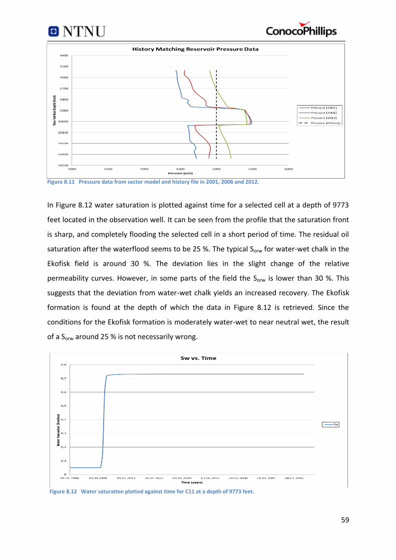
___________________________________________________________________________
59
Figure 8.12 Water saturation plotted against time for C11 at a depth of 9773 feet.
Figure 8.11 Pressure data from sector model and history file in 2001, 2006 and 2012.
In Figure 8.12 water saturation is plotted against time for a selected cell at a depth of 9773
feet located in the observation well. It can be seen from the profile that the saturation front
is sharp, and completely flooding the selected cell in a short period of time. The residual oil
saturation after the waterflood seems to be 25 %. The typical Sorw for water-wet chalk in the
Ekofisk field is around 30 %. The deviation lies in the slight change of the relative
permeability curves. However, in some parts of the field the Sorw is lower than 30 %. This
suggests that the deviation from water-wet chalk yields an increased recovery. The Ekofisk
formation is found at the depth of which the data in Figure 8.12 is retrieved. Since the
conditions for the Ekofisk formation is moderately water-wet to near neutral wet, the result
of a Sorw around 25 % is not necessarily wrong.

___________________________________________________________________________
60
Figure 8.13 Pressure plotted against time for C11 at a depth of 9773 feet.
Figure 8.14 Pressure plotted against time for C11 at a depth of 9873 feet.
The pressure profile, pressure plotted against time, is presented in Figure 8.13. The same cell
as in Figure 8.12 is used. The pressure build up starts in year 2003, which is somewhat late
compared to the data from the observation well. Judging from the profile, a reservoir
pressure of 5000 psia is not reached until year 2011. It reaches a plateau pressure of 5400
psia in year 2029. Considering that the pressure buildup profile in Figure 8.5 is an average
representation of the whole well, the model is not necessarily wrong. It should be sufficient
to reach a pressure greater than 5000 psia by 2014 for the purpose of this study.
If a cell at a greater depth is considered, as in Figure 8.14, the profile looks different due to
gravity effects. At this depth the pressure build up starts in year 1999, which is not far from
the reality. The pressure is 5000 psia in year 2006, and reaches a plateau value of 5350 psia
by 2025.

___________________________________________________________________________
61
Figure 8.15 Location (grey area) and design of the grid refinement (right).
8.4.1 Grid Refinement
For the simulation of the single well chemical tracer test only a small section of the history
matched model is to be used. A 20 feet interval of C11 in z-direction is to be perforated, and
the tracer is to be displaced 30 feet into the reservoir on both sides of the well. This 20 feet
times 60 feet interval, plus a buffer zone, making it 70 feet times 40 feet, was decided to
have grid cells the size of 1 foot in each direction. An image of the fine grid and its location
(in grey) can be seen in Figure 8.15. The fine grid, featuring a porosity map, is presented on
the right hand side. The yellow layers have a porosity of 35 %, while the red layers have 40 %
porosity. The fine grid is flanked by gradually increasing grid block sizes to make the model
more stable.
The placement of the test area is no coincidence. In order to be most assured matrix flow,
the layer flooded last in the flooding sequence was chosen. This area is located in the Upper
Tor Formation. The initial water saturation in the test area was 5 %. Permeability was 13 md
in x-direction, and 5 md in z-direction. The porosity was 35 % for the upper 15 feet, and 40%
for the lower 5 feet.
The reservoir temperature was fixed at 268 F. Allowing heat calculations lead to severe
instability in the model; hence it was removed. This decision was supported by the fact that
no cooling near C11 was seen during the last survey in 2012. It is safe to assume that no
cooling effect will take place near the wellbore when injecting cold water into C11 at the

___________________________________________________________________________
62
depth chosen. The slow injection rate combined with the large depth will most likely cause
the water to be heated up close to reservoir temperature by the time it reaches the
perforations.

___________________________________________________________________________
63
9 Single Well Chemical Tracer Test (SWCTT)
This chapter addresses the general function of a tracer, a single well chemical tracer test
(SWCTT) and how this can be used to determine the effect of a surfactant flood. Bear (1972)
defined a tracer as a “labeled portion of the same liquid which may be identified by its
density, color, electrical conductivity, etc.” In this thesis the tracer is identified by its salinity,
and solution chemistry and hydrolysis is not accounted for. The fine gridded area from
Chapter 8 was used for the simulations.
9.1 The Function of a SWCTT
When considering mature oil fields for application of EOR, two of the main challenges are
determining the amount of remaining oil, and evaluating the effect of EOR in pilot studies.
Core analysis and well logging are the two most widely used methods for measuring the
residual oil saturations. Major faults in both these methods is the small reservoir volume the
results represent, as well as the large uncertainty involved (Deans et. al. 1973) and (Deans &
Ghosh 1994). A SWCTT has proven to be a safer and more stable way of providing these
unknowns. SWCTTs are a method of push-and-pull operation in a producer or injector. The
test is based on injection of a reactive partitioning tracer, an ester, into the reservoir. The
ester is displaced by tracer-free water to a target depth from the wellbore, and the well is
shut in. The tracer will dissolve partly in the water phase and partly in the oil phase. During
the shut-in period some of the ester dissolved in the water phase hydrolyses into alcohol.
This product tracer is only soluble in water (Skrettingland et al. 2011). The hydrolysis is
dependent on pH and temperature. Symbolically the reaction can be written as (Huseby et
al. 2012);
The test utilizes the difference in travel time between the injected ester and the alcohol
generated in-situ by hydrolysis. Once back production starts, the product tracer will follow
the water, while the passive tracer in the oil phase is delayed. The degree of this delay is
(9.1)

___________________________________________________________________________
64
Figure 9.1 Tracer profiles for active (EtOH) and passive (EtAc) tracer (COPNO Internal).
dependent on the oil saturation in place. A tracer profile is made from the returning tracer,
and is compared to previously observed back produced concentrations to find the oil
saturation. Figure 9.1 shows tracer profiles for an active tracer (EtOH) and a passive tracer
(EtAc).
If the oil saturation is close to the residual, which it often is in water-flooded regions, the low
values of kro will make the oil flow rates negligible compared to the water flow rates. The oil
saturation is then determined by the difference in retention time of an active and passive
water tracer;
Where tEtOH and tEtAc are the retention times of the active and passive tracer, respectively, So
is the oil saturation, and K is the partition coefficient of the active tracer. The greater the oil
saturation, the greater the difference in arrival times will be.
If this tracer test is done both prior to- and after an EOR implementation is carried out, a
reduction in Sorw will be possible to observe. The tracer profile is measured in produced
volume (m3) vs. concentration of tracer (ppm). Sorw can be measured in a 10 meter radius
from the well. A fundamental assumption for the SWCTT to be valid is that the tracers do not
affect the phase transport. If this is the case, the simulation of tracer transport can be
performed in a separate module decoupled from the reservoir simulation itself (Huseby et
al. 2012). Two tracer pilot tests have been conducted on the Norwegian Continental Shelf;
one in the Snorre field, and one in the Heidrun field.
(9.2)

___________________________________________________________________________
65
The well options for the SWCTT are an existing injector, producer, infill injector or infill
producer. If an existing injector is used for the test there is a reduced chance of non-pilot oil.
On the other hand the near wellbore area has seen very high pressures and rates; hence
could have a too low Sorw, be very cold and be extensively fractured. The injector would also
need to have production capability for the back-production of the tracer. By using a
producer for the SWCCT there is a high chance for non-pilot oil unless a new well or a high
water cut well is used. The well would need to have injection capability. Injection into a hot
near wellbore area will create a temperature profile, affecting the tracer profile. This
temperature profile would most likely also be an issue with an infill producer, although not
in the same scale. An infill injector would presumably also be positioned in a water flooded
area like an existing injector, but with more intermediate temperatures (COPNO Internal).
9.2 Geological Effect on Tracer Curves
A simulation study was conducted with the aim to determine the geological effect on the
shape of the back produced tracer curves. Two cases of tracer injection are presented. In
one case, tracer was injected for 1.5 months followed by 0.5 months of chase water. In a
second case, tracer was injected for 1 month followed by 1 month of chase water. In reality
the tracer slug would be much smaller, but the large volume is chosen for viewing purposes.
After the two months of injecting was complete, the well was switched from an injector to a
producer. The tracer containing water was then back produced to obtain the tracer profile.
The purpose of the chase water was to attain a curve with a distinct top. The back produced
tracer was plotted as traced water (fraction) against time (days). The tests were carried out
in an area flooded to the residual oil saturation.
9.2.1 Two Extreme Geological Base Cases
Several different geology scenarios were run for two extreme base cases: (1) a completely
confined test area and (2) an unconfined test area. For the unconfined area, the tracer was
free to flow in every direction from the injector, while fluid flow for the confined test area
was restricted to flow within the horizontal boundaries of the 20 feet high perforation

___________________________________________________________________________
66
Figure 9.2 Tracer maps for confined (left) and unconfined (right) test areas after 2 months of injection.
Figure 9.3 Water injection rate plotted against time for confined (red) and unconfined (blue) cases.
interval. Fluid flow was restricted by applying a vertical permeability of 0.001 md to a single
layer above and under the perforated interval. Figure 9.2 presents the water tracer
propagation after injecting tracer for 1 month followed by 1 month of chase water. The scale
from 0 to 1 incorporated into the picture is used for all the maps of tracer concentration in
this chapter.
When the fluid flow was not restricted to the height of the perforation interval, the flow
propagated about 12 feet in z-direction from the top and bottom perforation. At the same
time the tracer propagated further away from the wellbore in x-direction. This behavior
suggests a higher injection rate for the unconfined case compared to the confined case.
Injection data confirmed that the injectivity much higher for the unconfined case (Figure
9.3). A possible explanation is that for the unconfined test area, more volume in different
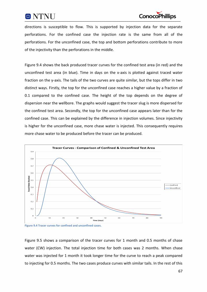
___________________________________________________________________________
67
Figure 9.4 Tracer curves for confined and unconfined cases.
directions is susceptible to flow. This is supported by injection data for the separate
perforations. For the confined case the injection rate is the same from all of the
perforations. For the unconfined case, the top and bottom perforations contribute to more
of the injectivity than the perforations in the middle.
Figure 9.4 shows the back produced tracer curves for the confined test area (in red) and the
unconfined test area (in blue). Time in days on the x-axis is plotted against traced water
fraction on the y-axis. The tails of the two curves are quite similar, but the tops differ in two
distinct ways. Firstly, the top for the unconfined case reaches a higher value by a fraction of
0.1 compared to the confined case. The height of the top depends on the degree of
dispersion near the wellbore. The graphs would suggest the tracer slug is more dispersed for
the confined test area. Secondly, the top for the unconfined case appears later than for the
confined case. This can be explained by the difference in injection volumes. Since injectivity
is higher for the unconfined case, more chase water is injected. This consequently requires
more chase water to be produced before the tracer can be produced.
Figure 9.5 shows a comparison of the tracer curves for 1 month and 0.5 months of chase
water (CW) injection. The total injection time for both cases was 2 months. When chase
water was injected for 1 month it took longer time for the curve to reach a peak compared
to injecting for 0.5 months. The two cases produce curves with similar tails. In the rest of this

___________________________________________________________________________
68
Figure 9.5 Tracer curves – Comparison of 1 & 0.5 months of chase water injection. Confined.
chapter the case of 1 month tracer injection followed by 1 month of chase water will be
used.
9.2.2 Introduction of a High Permeability Layer
One of the main points of research was how the tracer profile would be affected by a change
in geology. A high permeability layer (a fracture like feature) was introduced to the test area.
For the confined case, the fracture was incorporated into the middle of the test zone. The
unconfined case was given a high permeability layer three feet above the top perforation.
The horizontal permeability for this particular layer was varied between 20 md, 50 md, 200
md and 1000 md. Note that the horizontal permeability in the rest of the test area was 13
md. The vertical permeability was fixed at 5 md.
By simulating the different scenarios and viewing the tracer concentration map in CView
(viewing program for PSim), an idea of how far the fluid propagated into the reservoir
through the fracture was visualized. The results for the confined case can be seen in Figure
9.6. All of the images are captured after the 2 months of injection, and feature the scenario
of 1 month of tracer injection followed by 1 month of chase water. The red boxes indicate
the fine gridded test area of 70 feet times 40 feet.

___________________________________________________________________________
69
Figure 9.6 Tracer maps. Fracture with horizontal permeability 50 md (top), 200 md (middle) & 1000 md (bottom). Confined.
Figure 9.7 Tracer curves – Effect of fractures. Confined.
With the permeability of the fracture set to 20 md (not included in Figure 9.6), the tracer
stayed inside the test area, while it only slightly exceeded the boundary for the case of 50
md. For fracture permeabilities of 200 md and 1000 md, the tracer propagated as far as 175
feet and 455 feet respectively away from the wellbore.
Figure 9.7 shows the tracer curves for the cases presented in Figure 9.5, along with the base
case without the fracture. The case of the 50 md fracture produces a curve almost identical
to that of the base case. As the permeability of the fracture increases, the maximum back
produced tracer fraction decreases. The tops also shift slightly to the left. At the same time
the tail experiences a less steep decline.

___________________________________________________________________________
70
Figure 9.8 Tracer maps. Fracture with permeability 50 md (top), 200 md (middle) & 1000 md (bottom). Unconfined.
Figure 9.9 Tracer curves – Effect of fractures. Unconfined.
Similar trends were seen for the unconfined case with a fracture 3 feet above the
perforation interval (Figure 9.8), although the tracer did not propagate quite as far from the
test area.
Figure 9.9 shows the tracer curves for the cases in Figure 9.8, along with the base case for
the unconfined test area. Once again, the case of the 50 md fracture gives a similar curve as
the base case. The trend for the higher permeabilities is also the same; the maximum traced
water fraction decreases with increasing permeability, and the tops for the lower fractions
are shifted slightly to the left. The high permeability of the fracture allows tracer to be
produced earlier than for the base case.

___________________________________________________________________________
71
Figure 9.10 Tracer maps for when wells are shut in (left) and when wells are active (right). Confined.
9.2.3 The Effect of Active Wells in the Vicinity of the Test Area
All of the previous tracer tests were executed in a static environment. This was created by
shutting in the injector and producer on either side of C11 three years prior to the start of
tracer injection in C11. By shutting the wells in, the model stabilizes. In a real field,
conditions are not likely to be completely static. To see the effect of active wells around C11,
the injector and producer were left active. Apart from this, the injection scheme was the
same as for the previous cases. The results for the confined case are presented in Figure
9.10. Both images show the tracer maps after 2 months of injection, just prior to start of
back production. As expected, a clear drift towards the right is observed. This happens
because the net fluid flow in the model is from left to right when wells are active.
Viewing the back produced tracer profiles featured in Figure 9.11, it is clear that the case of
shut in wells reaches a higher top than the other case. The decline of the same curve is also
steeper. However, the case of active wells reaches the peak somewhat earlier. This is due to
the drift. Once tracer is injected on the left hand side of the well, it is met by a
countercurrent net fluid flow. Figure 9.10 clearly shows that the tracer concentration on the
left side of the well is higher for the case of active wells. When the tracer is back produced,
more of the tracer is produced at once. The same trends were observed when the same
scenario was run for the unconfined case.

___________________________________________________________________________
72
Figure 9.11 Tracer profiles for when wells are shut in (red) and when wells are active (blue). Confined.
Figure 9.12 Cumulative tracer when wells are shut in (red) and when wells are active (blue). Confined.
Figure 9.12 shows the cumulative amount of tracer retrieved by back production, and
confirms that more tracer is produced at once in the case of active wells. The total amount
of back produced tracer is however higher for the case with static conditions. When wells
are shut in, 99% of the tracer is produced after 3 months. In comparison, only 84% of the
tracer is produced after 3 months when the wells in the vicinity are kept active. The drift to
the right prevents all of the tracer from travelling back to the wellbore within the given
production period.

___________________________________________________________________________
73
10 Introducing Surfactants to the Model
This chapter includes an introduction to the basic logistics of a surfactant flood and
surfactant modelling in both a 2D sector model and a 2D radial model. With the sector
model the aim was to visualize how the surfactant slug mobilized a new oil bank. The goal
with the radial model was to determine the volumes of chemicals and tracer needed to
reach target depth from the well, and the time span of the operation.
10.1 The Basic Logistics of a Surfactant Flood
The three key parameters in the economics of a surfactant flood were defined by Spinler &
Baldwin (2000) as incremental oil recovery, surfactant loss and surfactant cost. The
incremental oil recovery is the measure of success for any EOR method. Surfactant loss is
important because it affects the volume of chemicals needed for achieving an effective
process.
Apart from cost, there are several other challenges related to the surfactant pilot test in
Ekofisk. Low salinity water has previously not been injected into the field, and there is
uncertainty around its compatibility with the chalk matrix. The location of the test area is
another uncertainty. It could either be performed in the developed water flooded area as a
tertiary recovery method, or in the unflooded South Ekofisk as a secondary recovery
method. It is desirable to execute the test in an area without fractures, so that matrix flow is
allowed. This is easier said than done, but seems more likely in the undeveloped South
Ekofisk sector of the field.
The preferred optimum salinity for the surfactant formulation is in the range of 48 000 ppm
to 62 500 ppm. By using a soft seawater formulation, the optimum salinity window becomes
much wider than for that of normal seawater. In the early stages of the surfactant study on
Ekofisk, the narrow optimum salinity window for seawater was a possible showstopper for
the pilot test. The immobile oil saturation will not be as effectively reduced without the type
3 phase behavior in the optimum salinity region.

___________________________________________________________________________
74
For normal seawater pH is in the range of 9 to 9.5, and the chalk surface is negatively
charged. For the modified seawater formulation pH is 11.5, and the surface change of chalk
is positive. The pH of the water was raised both to achieve optimum salinity and to reduce
adsorption. The latest measured surfactant adsorption value was 0.40 mg/g at a
temperature of 268 F. A previous value of 0.64 mg/g was measured at a lower temperature.
Because these values were not measured from Ekofisk chalk, an adsorption value of 1.6
mg/g will also be used in this thesis - as a possible high value.
It is desired that the solubilization ratio should be 10 or higher. This corresponds to an IFT in
the range of 0.003 dynes/cm or less (Levitt et al. 2009). A compromise must be made
between maximum solubilization ratio (low IFT), low viscosity and other factors required for
good transport. Polymer as a mobility buffer is not an option for Ekofisk due to the low
matrix permeability. Polymer molecules are so large that shear degradation would quickly
lower the viscosity to a point of inefficiency.
Another challenge is the temperature gradient that exists in the reservoir. The injection of
unheated seawater over a long period of time has cause a temperature gradient. Cooling
first appears in the vicinity of the injection wells, and a thermal front then moves through
the reservoir. A decrease in temperature will lead to a decrease in IFT, which will benefit the
viscous displacement of oil near the injection wells. The temperature gradient for Ekofisk
ranges from 60 F to 268 F. The current surfactant formulation has proved to have good
aqueous stability at both 155 F and 268 F. The thermal front should therefore not be an
issue.
10.2 Surfactant Flooding in a 2D Sector Model
A surfactant flood model was created by including a CEOR module (see appendix) in the
same model as for the tracer study in Chapter 9. Surfactant was injected for one month, and
was then followed by one month of chase water. The following back production then lasted
for 3 months. The bottom hole pressure (BHP) was 4000 psia for the producer and 7000 psia
for the injector. Surfactant was added to water with a salinity of 58 000 ppm. The optimum
salinity for the specific surfactant ranges between 0.821 meq/ml [48 000 ppm] (lower),
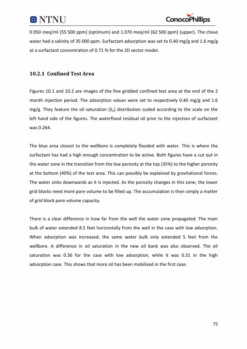
___________________________________________________________________________
75
0.950 meq/ml [55 500 ppm] (optimum) and 1.070 meq/ml [62 500 ppm] (upper). The chase
water had a salinity of 35 000 ppm. Surfactant adsorption was set to 0.40 mg/g and 1.6 mg/g
at a surfactant concentration of 0.71 % for the 2D sector model.
10.2.1 Confined Test Area
Figures 10.1 and 10.2 are images of the fine gridded confined test area at the end of the 2
month injection period. The adsorption values were set to respectively 0.40 mg/g and 1.6
mg/g. They feature the oil saturation (So) distribution scaled according to the scale on the
left hand side of the figures. The waterflood residual oil prior to the injection of surfactant
was 0.264.
The blue area closest to the wellbore is completely flooded with water. This is where the
surfactant has had a high enough concentration to be active. Both figures have a cut out in
the water zone in the transition from the low porosity at the top (35%) to the higher porosity
at the bottom (40%) of the test area. This can possibly be explained by gravitational forces.
The water sinks downwards as it is injected. As the porosity changes in this zone, the lower
grid blocks need more pore volume to be filled up. The accumulation is then simply a matter
of grid block pore volume capacity.
There is a clear difference in how far from the well the water zone propagated. The main
bulk of water extended 8.5 feet horizontally from the well in the case with low adsorption.
When adsorption was increased, the same water bulk only extended 5 feet from the
wellbore. A difference in oil saturation in the new oil bank was also observed. The oil
saturation was 0.36 for the case with low adsorption, while it was 0.31 in the high
adsorption case. This shows that more oil has been mobilized in the first case.

___________________________________________________________________________
76
Figure 10.2 So distribution after 2 months injection. (Ads=1.6 mg/g). Confined.
Figure 10.1 So distribution after 2 months injection. (Ads=0.40 mg/g). Confined.
10.2.2 Unconfined Test Area
Figures 10.3 and 10.4 show the So distribution for the unconfined case at the end of the
injection period. The injection rate is higher for the unconfined case, meaning both the
water zone and the oil bank has extended further away from the well than for the confined
case. Here there were 3 cut outs in the completely swept zone. The middle one is probably
the same as for the confined case. The top and bottom one could possibly be explained by
the same concept. The injectivity is higher for the top and bottom perforations than for the
middle ones. This water then sinks downwards, and since the permeability in x-direction is
higher than in z-direction, it starts to propagate outwards.

___________________________________________________________________________
77
Figure 10.4 So distribution after 2 months injection. (Ads=1.6 mg/g). Unconfined.
Figure 10.3 So distribution after 2 months injection. (Ads=0.40 mg/g). Unconfined.
The shape of the oil saturation distribution is similar for both the adsorption values. The case
with the low adsorption has extended further from the well than the case of high
adsorption. In addition, the oil saturation in the new oil bank was higher for the case of low
adsorption – as in the confined cases. The oil saturation in the low adsorption case was 0.36,
and extended 52 feet from the wellbore. The oil saturation was 0.31 in the new oil bank in
the case of high adsorption; extending 42 feet from the well.
The main bulk of water extended 12 feet in x-direction where the low adsorption value was
applied, whereas it extended 9 feet where the high adsorption was applied.

___________________________________________________________________________
78
Figure 10.6 Water injection- and oil production rates for unconfined case with and without surfactant.
Figure 10.5 Water injection- and oil production rates for confined case with and without surfactant.
Figures 10.5 and 10.6 display the water injection rates (blue) and oil production rates (green)
for the confined cases (Figure 10.5) and unconfined cases (Figure 10.6) with and without the
addition of surfactant. The full lines represent the cases with surfactant and an adsorption
value of 0.40 mg/g, the dashed lines represent the cases with surfactant and an adsorption
value of 1.6 mg/g, while the dotted lines represent water flooding without surfactant.
Water- and oil rates are plotted against time in days.

___________________________________________________________________________
79
Figure 10.7 Relative permeability and the effect of decreasing water saturation.
The same trends are observed for the two cases. Both water injectivity and oil production
increased when surfactant is added to the system. The increase was largest for the
unconfined case, and injection rates as well as production rates were overall higher. The oil
rate increased because the surfactant slug mobilized a new oil bank which was later back
produced.
The increase in injectivity can be explained by the behavior of the relative permeability
curves. Because the surfactant causes the formation of microemulsions, the surfactant slug
has higher viscosity than both oil and water. This would suggest that injectivity should be
lower when chemicals are added to the water. The formation of a new oil bank is also a
process working against increased injectivity. When the oil saturation increases, the position
on the relative permeability curves is moved to the left. This behavior can be seen in Figure
10.7. When the relative permeability to water decreases, so does the effective permeability
of water; making it harder to inject. Since this is not the case, a process must be overriding
the said effects.
When surfactant is added to the system, a new set of relative permeability curves becomes
active in the region where the surfactant works. The curves applied during low IFT conditions
are presented by dashed lines in Figure 10.8. They show that the residual oil saturation after
the chemical flood, Sor,CEOR, is 0 % as long as the surfactant is active. As the water saturation

___________________________________________________________________________
80
Figure 10.8 Relative permeability and the effect of low IFT conditions on water injectivity.
increases, the relative permeability to water increases drastically. This explains the increased
injectivity observed from the graphs in Figure 10.5 and 10.6.
10.2.3 Residual Oil Distribution
Core experiments done in the Bartlesville laboratory showed less than 10 % residual oil
saturation after the core had been flooded with surfactants. Moving forward, a Sorw of 9 %
will be used for this thesis. However, how the Sorw was distributed inside the core was not
initially recognized. It was first believed that the entire residual oil saturation was
accumulated close to the producer. This concept is illustrated by Figure 10.9. The core in
question was later sliced open. Visual inspection then indicated that the oil was evenly
distributed throughout the length of the core. This latter concept is illustrated by Figure
10.10.
Figure 10.9 shows the concept being used in the simulation model. The water saturation is
100 %, governed by the low IFT relative permeability curves, as long as the surfactant
concentration is high enough for it to be active. When the concentration falls below the
critical value, the system switches back to the relative permeability curves for normal
conditions. In this particular case, this leaves a residual oil saturation of 30 % in the rest of

___________________________________________________________________________
81
Figure 10.9 Model representation of the fluid distribution inside a core.
Figure 10.10 Presumably the correct representation of the fluid distribution inside a core.
the reservoir; summing up to a total of 9 % residual oil. It could be argued that this is a
misleading representation of the situation.
Applying this concept would mean that if the injector and producer are just placed close
enough, the oil recovery would be 100 % in the whole reservoir. This may look wrong,
knowing that there is supposed to be 9 % residual oil left after the surfactant flood. A more
reasonable representation of the core can be seen in Figure 10.10.
In this latter figure, the residual oil is spread out uniformly through the entire core. To
achieve this, a new set of relative permeability curves for low IFT conditions would need to
be implemented. For this new curve the relative permeability to water should reach a
maximum of 91 % water saturation. Present limitations in PSim prevent this from being
applied to the model. It is currently being worked on by the developers of PSim.

___________________________________________________________________________
82
10.3 Surfactant Flooding in a 2D Radial Model
The objective of studying a 2D radial model was to determine the volumes necessary to
create an effective SWCTT. The injection scheme is presented in Table 10.1. The middle of
the tracer slugs should be displaced 10 feet into the reservoir. This proved to correspond to
the end of the slug being placed 12 feet away from the well. The surfactant slug should be
displaced 20 feet from the well. Predetermined slug volumes of 0.1 PV for both tracers were
to be injected prior to – and after the surfactant slug. In the field, two short shut in periods
after the tracer placement would be required for tracer hydrolysis. The tracer in the
simulation model does however not react; hence it does not need the shut in period.
A 2D radial model for Ekofisk was created with 200 cells in x-direction (2000 feet) and three
layers. Since the model is radial, the volumes of the grid blocks increase exponentially away
from the well. A single well, placed in the middle of the model, operated as both injector and
producer. The applied salinity gradient ranged between 58 000 ppm and 28 000 ppm. Water
viscosity was set to 0.2214, and initial water saturation was 70 %. This implied that the area
in question had already been flooded with water. Porosity was 40 % in all layers,
permeability in x- and z-direction was 4 md, and transmissibility was 1 in both directions.
Two different values for surfactant adsorption were used for the surfactant concentration of
0.71 %; 0.40 mg/g and 1.6 mg/g. These adsorption values correspond to retention numbers
of 0.16% and 0.64% respectively. The values are within the range determined by laboratory
core experiments and simulation studies done in Bartlesville, OK.
10.3.1 Flow Scheme to Determine Slug Volumes
A flow scheme for the SWCTT was created based on the core experiments and simulation
studies. The pore volume of surfactant needed to reach a distance of 20 feet from the well is
highly dependent on the retention number. To determine the effect of adsorption, two
scenarios of retention numbers were run.

___________________________________________________________________________
83
Table 10.1 Schedule for the SWCTT (Adsorption = 0.4 mg/g)
Step Operation PV BBLS DAYS L res.
Preflush INJ 0,50 895 25,6
Tracer 1 INJ 0,10 179 5,1 12
Placement 1 INJ 0,18 322,2 9,2
Flowback 1 PROD 0,38 680,2 19,4
Cleaning INJ 0,50 895 25,6
SF Slug INJ 0,40 716 20,5 18
Placement SF INJ 1,05 1880 53,7
Tracer 2 INJ 0,10 179 5,1 12
Placement 2 INJ 0,27 483,3 13,8
Flowback 2 PROD 0,19 340,1 9,7
Total INJ 3,1 5549 159
Total PROD 0,6 1020 29
Total INJ&PROD 3,7 6569 188
Since the test zone was confined to a 20 x 20 feet radial interval, one pore volume (PV) can
be calculated as;
Water injection rate was fixed to 35 bbls/day. This rate was based on earlier simulation
studies. Table 10.1 shows the schedule for the single well chemical tracer test with 0.40
mg/g adsorption. The bold numbers in the PV column are fixed volumes, and were not
altered to get the slugs to the desired distance from the well. The volume of chase water
behind the tracer slugs was, however, altered to place the tracer at the right distance. The
pore volume of chase water behind the surfactant slug was also fixed. A larger volume of this
slug proved to make no difference in placing the surfactant slug further from the well.
Adsorption reduced the tracer concentration to ineffective long before the entire PV of
placement water had been injected.
The reservoir was preflushed with 0.5 PV of 35 000 ppm salinity water. The preflush was
followed by 0.1 PV of tracer in form of 58 000 ppm salinity water. The tracer was displaced
12 feet from the well by 0.18 PV of 35 000 ppm salinity water. The injector was then
switched to a producer for a 0.33 PV back production of the tracer. The next step was a
cleaning process by means of injecting 0.5 PV of 35 000 ppm salinity water. This was
(10.1)

___________________________________________________________________________
84
Figure 10.11 So, water salinity and SF concentration in the water phase 6 feet from the well. (Adsorption = 0.4 mg/g)
followed by the injection of the surfactant slug in 58 000 ppm salinity water. Applying the
adsorption value of 0.40 mg/g proved to displace the effective surfactant slug out to a radius
of 18 feet. After the placement of the surfactant slug, the second tracer of 0.1 PV was
injected. This was displaced by 0.27 PV for the middle of the slug to reach a depth of 10 feet
from the well. The injector was again switched to a producer; back producing 0.19 PV.
Using the same volumes and an adsorption value of 1.6 mg/g proved to only displace the
surfactant slug to a depth of 13 feet from the well (see appendix). A third scenario with an
adsorption value of 0.64 mg/g can also be found in the appendix. The whole process took 6
months to complete.
Figure 10.11 shows the oil saturation (dashed red), water salinity (green) and surfactant
concentration partitioned in the water phase (black) plotted against time (days). The oil
saturation and water salinity scale is featured on the left hand side, while the scale on the
right hand side is for the surfactant concentration.
These values were taken 6 feet from the wellbore. The first two green tops represent the
concentration of Tracer 1 as it is injected (first top) and back produced (second top). The
second tracer is not completely back produced, which is the reason for the second bump at
the end of it. The two last green tops represent injection and production of Tracer 2. The

___________________________________________________________________________
85
Figure 10.12 So, water salinity and SF concentration in the water phase 16 feet from the well. (Adsorption = 0.4 mg/g)
tracer comprises of high salinity water, which was also used for the injection of the
surfactant slug. The surfactant concentration top and the high salinity top nearly coincide
completely in terms of time. A small oil bank is pushed slightly ahead of the surfactant slug.
The oil saturation is immediately reduced to zero as the surfactant in combination with the
high salinity water reaches the depth of interest after 90 days.
Figure 10.12 shows the same scenario as Figure 10.11, but at a larger depth from the
wellbore. The surfactant slug is much more dispersed at a distance of 16 feet from the well,
and the fraction of high concentration surfactant is drastically reduced. It still manages to
reach a high enough concentration to effectively reduce the oil saturation to zero around
day 120.
The same type of profiles for adsorption values of 0.64 mg/g and 1.6 mg/g showed the same
trends. The surfactant was reduced to a concentration under the critical at distances of 16
feet and 13 feet from the well, respectively.

___________________________________________________________________________
86
Figure 10.13 Back produced tracer curve for 2D radial model.
The resulting back produced tracer curve is presented in Figure 10.13. It shows the traced
water fraction plotted against time in days. The first top is for Tracer 1, while the second is
for Tracer 2. The second tracer is slightly more dispersed than the first tracer; drawn out
from the lower value of the top. This can be linked to the larger volume of chase water
needed to displace the second slug to the desired depth.

___________________________________________________________________________
87
11 Conclusion and Discussion
To sum up the findings in this thesis, the following conclusions can be made:
1. The height of the tracer curve top depends on the degree of dispersion near the
wellbore. If the tracer slug becomes highly dispersed by water close to the well, the
top will reach a lower value than a more concentrated tracer slug.
2. The length and shape of the tracer curve tail depends on the degree of dispersion in
the tracer furthest away from the well. A higher degree of dispersion produces a tail
with higher traced water fraction than a lower degree of dispersion does.
3. The degree of dispersion increases with increasing heterogeneity, but does not affect
the smoothness of the curve.
4. Retention plays a major role in the volume of surfactant needed to design an efficient
SWCTT.
5. The surfactant slug becomes increasingly dispersed as it travels further from the well.
6. The surfactant slug reaches a depth of 18 feet with an adsorption of 0.4 mg/g with a
surfactant slug of 0.4 PV. A depth of 13 feet is reached with the same volumes and an
adsorption value of 1.6 mg/g. The total process takes 6 months.
Dispersion can be explained as the mixing caused by a single-phase fluid moving through a
porous medium. In a multiphase system diffusivity refers to the mixing of tracer within the
flow path of a given phase, not the mixing of the phases themselves (Miller 2010). The tracer
starts out with an abrupt interface, which gradually evolves into an ever-widening transition
zone. Across the transition zone the tracer concentration varies between that of the tracer
to that of the other liquid (Bear 1972).

___________________________________________________________________________
88
Figure 11.1 Breakthrough curves in a 1D flow in a sand column. After Bear (1972).
Figure 11.1 features two breakthrough curves for one-dimensional flow in a sand column.
Relative tracer distribution (ε) on the y-axis is plotted against time (Qt/U0), where U0 is the
pore volume of the column and Qt is the constant discharge rate. The dashed line represents
an ideal flow without dispersion. This kind of flow front is called a shock front. The full line
represents the actual flow front with dispersion, and is characterized by an S-shaped curve.
The effect of fractures was seen clearly for both the confined and the unconfined test area.
As the fracture permeability increased, more tracer bearing water escaped from the test
area; reducing the height of the tracer curve tops. The traced water fraction of the tail
increased as the fracture permeability increased. These two features indicate a higher
degree of dispersion in both ends of the tracer slug as the permeability of the fracture
increased. This coincides with the statement from the literature that heterogeneity leads to
more dispersion. The increase in dispersion as heterogeneity increased was largest for the
confined test area. This may be due to the difference in placement of the fracture for the
two cases, or the fact that a smaller area is more sensitive to change.
The result of active wells in the vicinity of the test area was a clear drift in the net fluid flow
direction. Based on the tracer curves for this case, the drift caused a high degree of
dispersion in both ends of the slug. This effect was most prominent for the rear of the slug.
The shape of the curve will also be a function of the drift rate and shut-in time. The tracer
response could possibly separate into two tops with a high drift and a long shut-in time.

___________________________________________________________________________
89
Figure 11.2 Computed tracer curve and field data (Deans et. al. 1973).
All the tracer curves presented in this thesis are smooth with a single top. In some cases
tracer curve tops with structure are experienced, as can be seen in Figure 11.2.
This simulation study suggests that reservoir heterogeneity will not produce tracer curves
with multiple tops. It should be noted that solution chemistry was not applied in the model,
hence it was suggested that multiple tops on tracer curves can be a result of the hydrolysis
that takes place either before or after the tracer slug has been displaced to the preferred
depth. Hydrolysis of the tracer starts immediately after the tracer comes in contact with
water; not only during the shut in period. The shape of the produced tracer profiles is
changed by the variations of hydrolysis rate with pH. The reaction velocity of an ester, the
hydrolysis rate, is catalyzed by both acids and bases. The rate increases both ways from a pH
of 6.5; where the rate is at a minimum (Deans & Ghosh 1994).
Acetic acid is produced during hydrolysis. If the rock does not have enough buffer capacity to
absorb the acid, the environment will become increasingly acidic; hence increasing the
hydrolysis rate. A consequence of the pH rate dependence of ester hydrolysis is that transit-
generated tracer may dominate the response; making the test insensitive to oil saturation. It
is desired that most of the tracer undergoes hydrolysis during the shut in period.
For the SWCTT to be applicable on Ekofisk, the time to complete the test needs to be
reduced. It lasts for 6 months as it is presented here. The preferred time is maximum 1-2
months. More studies on injection rate and adsorption need to be performed. If injection is
not substantially higher than the 35 bbl/day presented in this thesis, the depth at which the
slugs are to be displaced needs to be reduced.

___________________________________________________________________________
90

___________________________________________________________________________
91
11.1 Future Work and Limitations
Future work involves finding the final optimum surfactant formulation for Ekofisk chalk with
regards to environmental regulations, retention values, cost and availability. Ekofisk chalk
cores are being prepared for surfactant flooding as this thesis is being written. When the
results from these test become available, a more accurate model can be made with respect
to recovery and adsorption.
The appropriate flow scheme and necessary volumes need to be made clear. The volumes
presented in this thesis are clearly too large. This could indicate that the chosen injection
rate is too low. Further studies need to be done regarding the injection rate that can be
expected for the appropriate well. The desired time for the entire SWCTT is 1 – 2 months.
Shorter displacement lengths of the slugs should be considered if the injection rates turn out
to be within the range presented in this thesis.
A location for the SWCTT needs to be chosen. The two main options currently being
considered are the water flooded areas or the unflooded areas of Ekofisk South. An ideal
test zone for the SWCTT should be thin and isolated with matrix flow. In reality there is no
way to assure that the chosen zone is ideal, and flow out of the zone is likely to occur. If an
existing well or a new well is to be drilled, also needs to be determined.
A choice also needs to be made with regards to performing a secondary or tertiary
surfactant flood. This choice is clearly co-dependent on the choice for well location.
Secondary recovery could be performed in the unflooded section of the reservoir, while
tertiary could be performed in the flooded areas.
Figure 11.3 shows the steps in a screening process for a general EOR technique. The process
uncertainty decreases as more steps are performed. The effort and investment also
increases significantly with each step in the process.

___________________________________________________________________________
92
Figure 11.3 Illustration of a flow chart for an EOR screening process (Schlumberger 2014).
The natural next step after the Ekofisk SWCTT would be a second SWCTT, a two-well pilot or
a multi well pilot. The two latter pilot tests are very costly. They take a lot of time; both the
planning, execution and the time it takes to see the response. The main goal of a two-well
pilot or a multi well pilot is to estimate the impact of heterogeneity.
A large amount of limitations are associated with the practical field implementation of a
surfactant flood. A great quantity of equipment and logistics is involved in the process. One
particular limitation is the logistics around finding a practical way to separate the emulsions
formed during a surfactant flood. If the water is to become clean enough to be discarded
back into the sea, these emulsions need to be efficiently handled.

___________________________________________________________________________
93
12 References
Abe, M., Schechter, D., Schechter, R.S., Wade, W.H., Weerasooriya, U. and Yiv, S. 1986.
Microemulsion with Branched Tail Polyoxyethelene Sulfonate Surfactants. Journal of
Colloid and Interface Science 114 (2): 342-356.
Ahmed, T. and Meehan, D.N. 2012. Chapter 6 – Introduction to Enhanced Oil Recovery. In:
Ahmed, T. and Meehan, D. N. (eds.) Advanced Reservoir Management and Engineering
(Second Edition). Boston: Gulf Professional Publishing.
Ashraf, A., Hadia, N., Torsæter, O. and Tweheyo, M.T. 2010. Laboratory Investigation of Low
Salinity Waterflooding as Secondary Recovery Process: Effect of Wettability. Paper SPE
129012 presented at the SPE Oil and Gas India Conference and Exhibition, Mumbai, India,
20-22 January 2010.
Austad, T. 2013. “Smart Water” Flooding in Carbonates and Sandstones: A New Chemical
Understanding of the EOR-potential. UiS, Norway. Presented at the FORCE education
Seminar NPD, Nov. 6-7., 2013.
Austad, T., Strand, S., Madland, M. V., Puntervold, T. and Korsnes, R. I. 2008. Seawater in
Chalk: An EOR and Compaction Fluid. Paper IPTC 11370/ SPE 118431 presented at the
2007 International Petroleum Technology Conference, Dubai, 4-6 December.
Austad, T. and Milter, J. 1997. Spontaneous Imbibition of Water into Low Permeable Chalk at
Different Wettabilities Using Surfactants. Paper SPE 37236 presented at the International
Symposium on Oilfield Chemistry, Houston, TX, 18-21 February 1997.
Awan, A.R., Teigland, R. and Kleppe, J. 2008. A Survey of North Sea Enhanced-Oil-Recovery
Projects Initiated During the Years 1975 to 2005. Paper SPE 99546 presented at the 2006
SPE/DOE Symposium on Improved Oil Recovery, Tulsa 22-26 April.

___________________________________________________________________________
94
Bear, J. 1972. Dynamics of Fluids in Porous Media: American Elsevier Science Publishing Co.,
Inc. New York.
Brown, L.R., Vadie, A.A. and Stephens, O.J. 2002. Slowing Production Decline and Extending
the Economic Life of an Oil Field: New MEOR Technology. Paper SPE 75355 presented at
the 2000 SPE/DOE Improved Oil Recovery Symposium, Tulsa, 3–5 April.
Boyce, B.M. 1972. Ekofisk Phase 1 Production Looks Good, Oil & Gas J. (June 12, 1972)
Bryant, S.L. and Lockhart, T.P. 2002. Reservoir Engineering Analysis of Microbial Enhanced Oil
Recovery. Paper SPE 79719 presented at the 2000 SPE Annual Technical Conference and
Exhibition, Dallas, 1–4 October.
Cinar, Y. Lectures in PTRL 4012/5012, Enhanced oil and gas recovery. UNSW. Spring 2013.
ConocoPhillips n.d. The Greater Ekofisk Area. Available at: www.conocophillips.no.
[26 March 2014].
COPNO Internal, Internal Database at ConocoPhillips Norwegian Business Unit.
[January-June 2014].
Cuiec, L., Bourbiaux, B. and Kalaydjian, F. 1994. Oil Recovery by Imbibition in Low-
Permeability Chalk. Paper SPE 20259 presented at the 1990 SPE/DOE Symposium on
Enhanced Oil Recovery in Tulsa, April 22-25.
Deans, H.A., Tomich, J.F., Dalton, R.L. and Shallenberger, L.K. 1973. Single-Well Tracer
Method To Measure Residual Oil Saturation. Paper SPE 3192 presented at SPE
Symposium on Improved Oil Recovery, Tulsa, April 16 – 19, 1972.
Deans, H.A. and Ghosh, R. 1994. pH and Reaction Rate Changes During Single-Well Chemical
Tracer Tests. Paper SPE/DOE 27801 presented at the SPE/DOE Ninth Symposium on
Improved Oil Recovery, Tulsa 17 – 20 April, 1994.

___________________________________________________________________________
95
Elshahawi, H., Fathy, K. and Hiekal, S. 1999. Capillary Pressure and Rock Wettability Effects
on Wireline Formation Tester Measurements. Paper SPE 56712 presented at the 1999 SPE
Technical Conference and Exhibition held in Houston, Texas, 3-6 October 1999.
Ersland, G., Ferno, M. A., Graue, A., Baldwin, B.A. and Stevens, J. 2010. Complementary
imaging of oil recovery mechanisms in fractured reservoirs. Chemical Engineering Journal,
158, 32-38.
FORCE Report 2011, Assessment of Environmental Impact from EOR Chemicals for the
Norwegian Continental Shelf, Available from: www.force.org. [25 February 2014].
Grigg, R.B. and Mikhalin, A.A. 2007. Effects of Flow Conditions and Surfactant Availability on
Adsorption. Paper SPE 106205 presented at the 2007 SPE International Symposium on
Oilfield Chemistry, Houston, Tx, 28 February – 2 March.
Hallenbeck, L.D., Sylte, J.E., Ebbs, D.J. and Thomas, L.K. 1991. Implementation of the Ekofisk
Field Waterflood. Paper SPE 19838 presented at the 1989 SPE Annual Technical
Conference and Exhibition, San Antonio.
Healy, R.N. and Reed, R.L. 1974. Physiochemical Aspects of Microemulsion Flooding. Paper
SPE 4583 presented at the SPE-AIME 48th Annual Fall Meeting, Las Vegas, Nev., Sept. 30
– Oct. 3, 1973.
Hearn, C.L. 1971. Simulation of Stratified Waterflooding by Pseudo Relative Permeability
Curves. Paper SPE 2929 presented at SPE 45th Annual Fall Meeting, Houston, Oct. 4 – 7,
1970 and at SPE Petroleum Technology Symposium, Hobbs, Oct. 29 - 30, 1970.
Hermansen, H., Landa, G. H., Sylte, J. E. and Thomas, L. K. 2000. Experiences after 10 years of
waterflooding the Ekofisk Field, Norway. Journal of Petroleum Science and Engineering,
26, 11-18.

___________________________________________________________________________
96
Hirasaki, G.J., Miller, C.A. and Puerto, M. 2011. Recent Advances in Surfactant EOR. Paper
SPE 115386 presented at the SPE Annual Technical Conference and Exhibition, Denver,
21-24 September 2008.
Horikx, J.T., Timmermans, P., Daudin, R., O`Neill, N. and Sorriaux, F. M. 2013. A Specific Way
of Assessing Target Recovery Factor (Chalk Oil Fields). Paper IPTC 16925 presented at the
2013 International Petroleum Technology Conference, Beijing, China, 26-28 March.
Huseby, O.K., Sagen, J. & Dugstad, O. 2012. Single Well Chemical Tracer Tests – Fast and
Correct Simulations. Paper SPE 155608 presented at the SPE EOR Conference at Oil and
Gas West Asia held in Muscat, Oman, 16-18 April 2012.
Jensen, T.B., Harpole, K. J. and Østhus, A. 2000. EOR Screening for Ekofisk.Paper SPE 65124
presented at the SPE European Conference held in Paris, France, 24-25 October 2000.
Lake, L.W. 1987. Chemical Flooding (1987 PEH Chapter 47) U. of Texas 1987-47-PEH 1987.
Society of Petroleum Engineers PEH SPEBOOK.
Lake, L.W. 1989. Enhanced Oil Recovery. Englewood Cliffs, New Jersey: Prentice Hall.
Levitt, D.B., Jackson, A.C., Heinson, C., Britton, L.N., Malik, T., Dwarakanath, V. and Pope,
G.A. 2009. Identification and Evaluation of High-Performance EOR Surfactants. Paper SPE
100089 presented at the SPE/DOE Symposium on Improved Oil Recovery, Tulsa 22-26
April 2006.
Miljødirektoratet 2013, Olje og Gass. Available from: http://www.miljostatus.no/Tema/Hav-
og-kyst/Olje-og-gass. [25 February 2014].
Miller, M. 2010. Naturally Fractured Reservoir Engineering Course Material. HOT course held
in Vienna, Austria, Sept. 27 – Oct. 1, 2010.

___________________________________________________________________________
97
Morrow, N. and Buckley, J. 2011. Improved Oil Recovery by Low-Salinity Waterflooding.
Paper SPE 129421. Distinguished Author Series.
Morrow, N.R. and Mason, G. 2001. Recovery of Oil by Spontaneous Imbibition. Current
Opinion in Colloid & Interface Science, 6, 321-337.
Nelson, R.C., Lawson, J.B., Thigpen, D.R. and Stegemeier, G.L. 1984. Cosurfactant-Enhanced
Alkaline Flooding. Paper SPE 12672 presented at the SPE Enhanced Oil Recovery
Symposium, Tulsa, 15-18 April.
Newman, G.H. 1983. The Effect of Water chemistry on the Laboratory Compression and
Permeability Characteristics of Some North Sea Chalks. Paper SPE 10203 presented at the
1981 SPE Annual Technical Conference and Exhibition, San Antonio, Oct. 5-7.
NPD, Norwegian Petroleum Directorate. Available from: www.npd.no. [19 February].
Robertson, S.D. 1988. An Empirical Model for Microemulsion Phase Behavior. Paper SPE
14909 presented at the 1986 SPE Symposium on Enhanced Oil Recovery in Tulsa, April
20-23.
Saud, S.A. and Abdulaziz, A.A. 1998. Factors affecting pseudo relative permeability curves.
Journal of Petroleum Science and Engineering, Volume 21, Issue 3 – 4, [249-261].
Schlumberger, 2014. Available from: www.slb.com. [3 June 2014].
Sheng, J.J. 2013. Chapter 12 – Surfactant Enhanced Oil Recovery in Carbonate Reservoirs. In:
Sheng, J.J. (ed.) Enhanced Oil Recovery. Field case studies. Boston: Gulf Professional
Publishing.
Sheng, J.J. 2012. Synergistic Mechanisms of ASP Flooding. Available from:
http://www.upstreampumping.com/article/production/synergistic-mechanisms-asp-
flooding. [16 November 2013].

___________________________________________________________________________
98
Sheng, J.J. 2011. Chapter 7 – Surfactant Flooding. In: Sheng, J.J. (ed.) Modern Chemical
Enhanced Oil Recovery. Boston: Gulf Professional Publishing.
Siggel, L., Santa, M., Hansch, M, Nowak, M., Ranft, M., Weiss, H., Hanjal, D., Schreiner, E.,
Oetter, G. and Tinsley, J. 2012. A New Class of Viscoelastic Surfactants for Enhanced Oil
Recovery. Paper SPE 153969 presented at the Eighteenth SPE Improved Oil Recovery
Symposium held in Tulsa, Oklahoma, USA, 14-18 April 2012.
Skauge, A. 2013. EOR-Introduction. Presented at the FORCE – EOR Competence Building
Seminar, 6-7 November, Stavanger, Norway. Available from: www.force.og.[24
February].
Skrettingland, K., Holt, T., Tweheyo, M. T. and Skjevrak, I. 2011. Snorre Low Salinity Water
Injection –Core Flooding and Single Well Field Pilot. Paper SPE 129877, SPE Reservoir
Evaluation & Engineering, Vol 14, No. 2, pp. 182-192, 2011.
Solairaj, S., Britton, C., Kim, D.H., Weerasooriya, U. and Pope, G. A. 2012. Measurement and
Analysis of Surfactant Retention. Paper SPE 154247 presented at the Eighteenth SPE
Improved Recovery Symposium, Tulsa, Oklahoma, USA, 14-18 April 2012.
Spinler, E.A. and Baldwin, B.A. 2000. Surfactant Induced Wettability Alteration in Porous
Media. In: L.L. Schramm (Editor), Surfactant Fundamental and Application in the
Petroleum Industry. Cambridge University Press, pp. 159-202.
SSB 2014, Oil and gas activities, production, Q4 2013. Statistics Norway. Available from:
www.ssb.no. [15 May 2014].
Sulak, R.M. 1990. Ekofisk Field: the first twenty years. Paper SPE 20773 presented at the
1990 SPE Annual Technical Conference, New Orleans, September 23-26.
Surkalo, H. 1990. Enhanced Alkaline Flooding. Paper SPE 19896. Technology Today Series.

___________________________________________________________________________
99
Taber, J.J., Martin, F.D. and Seright, R.S. 1997. EOR Screening Criteria Revisited - Part 1:
Introduction to Screening Criteria and Enhanced Recovery Field Projects. Paper SPE 35385
presented at the 1996 SPE/DOE Improved Oil Recovery Symposium, Tulsa, Oklahoma, 21-
24 April.
Tiab, D. and Donaldson, E.C. 2012. Chapter 5 – Capillary Pressure. Petrophysics (Third
Edition). Boston: Gulf Professional Publishing.
Van den Bark, E. and Thomas, O.D. 1980. Ekofisk: First of the Giant Oil Fields in Western
Europe. Giant Oil and Gas Fields of the Decade, AAPG, Tulsa (1980) Memoir 30, 195-224.
Wang, J., Dong, M. and Arhuoma, M. 2010. Experimental and Numerical Study of Improving
Heavy Oil Recovery by Alkaline Flooding in Sandpacks. Paper SPE 134248 presented at
the 9th Canadian International Petroleum Conference June 17–19, 2008, Calgary,
Alberta.
Warren, J.E. and Root, P.J. 1963. The Behavior of Naturally Fractured Reservoirs. Paper SPE
426 presented at the Fall Meeting of the Society of Petroleum Engineers Oct. 7-10, 1962,
Los Angeles. Pittsburgh: Gulf Research & Development Co.
Winsor, P.A 1954. Solvent Properties of Amphiphilic Compounds. London: Butterworth`s
Scientific Publications.
Zahid, A., Stenby, E.H. and Shapiro, A.A. 2010. Improved Oil Recovery in Chalk: Wettability
Alteration or Something Else? Paper SPE 131300 presented at the SPE EUROPEC/EAGE
Annual Conference and Exhibition held in Barcelona, Spain, 14-17 June 2010.
Zhang, R. and Somasundaran, P. 2006. Advances in Adsorption of Surfactants and their
Mixtures at Solid/Solution Interfaces. Elsevier: Advances in Colloid and Interface Science.
Zolotukhin, A.B. and Ursin, J. 2000. Introduction to Petroleum Reservoir Engineering.
Høyskoleforlaget, Norwegian Academic Press.

___________________________________________________________________________
100

___________________________________________________________________________
101
Step Operation PV BBLS DAYS L res.
Preflush INJ 0,50 895 25,6
Tracer 1 INJ 0,10 179 5,1 12
Placement 1 INJ 0,18 322,2 9,2
Flowback 1 PROD 0,38 680,2 19,4
Cleaning INJ 0,50 895 25,6
SF Slug INJ 0,40 716 20,5 13
Placement SF INJ 1,05 1880 53,7
Tracer 2 INJ 0,10 179 5,1 12
Placement 2 INJ 0,27 483,3 13,8
Flowback 2 PROD 0,19 340,1 9,7
Total INJ 3,1 5549 159
Total PROD 0,6 1020 29
Total INJ&PROD 3,7 6569 188
Step Operation PV BBLS DAYS L res.
Preflush INJ 0,50 895 25,6
Tracer 1 INJ 0,10 179 5,1 12
Placement 1 INJ 0,18 322,2 9,2
Flowback 1 PROD 0,38 680,2 19,4
Cleaning INJ 0,50 895 25,6
SF Slug INJ 0,40 716 20,5 16
Placement SF INJ 1,05 1880 53,7
Tracer 2 INJ 0,10 179 5,1 12
Placement 2 INJ 0,27 483,3 13,8
Flowback 2 PROD 0,19 340,1 9,7
Total INJ 3,1 5549 159
Total PROD 0,6 1020 29
Total INJ&PROD 3,7 6569 188
A.X Schedule for the SWCTT (Adsorption = 0.64 mg/g)
A.X Schedule for the SWCTT (Adsorption = 1.6 mg/g)
Appendices
Flow Schemes at Different Adsorption Values

___________________________________________________________________________
102

___________________________________________________________________________
103
PSim Data Input File
TITLE
Ekofisk sector model 2 from south Ekofisk (P50 model)
Horizontal wells at 4000 bbl/day injection rate
Surfactant adsorption = 0.55 mg/g at surf conc. 0.71%
With salinity gradient: 80,000 ppm, 50,000 ppm, and 35,000 ppm
ENDTITLE
C ============================================================================
GRID 112 1 234
FIELDNAME Ekofisk sector 1
C ============================================================================
KEYWORD
DATE 1 1 1986
HISTORYFILE
C11_R_2.history
C ============================================================================
C === GENERAL FLUID PROPERTIES
C ============================================================================
C ----------------------------------------------------
C Water and rock properties
C ----------------------------------------------------
MISC 1.07 3.4e-006 59.554 0.2214 1e-005 14.7 ! Bwi cw denw visw Cr
Pref
C ----------------------------------------
C Standard pressure and temperature
C ----------------------------------------
PSTD 14.7
TSTD 60
C ============================
C Fluid EOS Properties
C ============================
PVTEOS
268.
CPT MW TC PC AC ZCRIT SHIFT PCHOR OMEGA OMEGB
OMEGAS OMEGBS
C1N2 16.12 341.7 665.8 .0119 .3594 -.15920 76.8 .5051080 .0777805
.5051080 .0777805
C2C3 35.70 596.6 703.6 .1257 .3290 -.10032 119.1 .4303043 .0796165
.4303043 .0796165
C4F1 79.48 908.4 468.9 .2619 .2361 -.00372 251.1 .4262349 .0749099
.4262349 .0749099
F2F3 180.89 1273.6 289.6 .5357 .2292 .11424 520.2 .4415066 .0758590
.4415066 .0758590
F4F5 408.17 1609.2 159.6 1.0469 .2460 .17074 944.4 .4382145 .0766369
.4382145 .0766369
BIN Interaction Parameters
.00988 .01270 .02670 .13800
.01050 .01180 .01180
.00000 .00000
.00000
HEATBALANCE ! 3
C cpw rocpf k tginj twinj rowinj
slope_bw0 res_ti
1. 37.2 30. 268. 268. 62.43
-.000336 268.
5.00000E-01 5.00000E-01 5.00000E-01 5.00000E-01 5.00000E-01
53.96 1.308
59 1.216

___________________________________________________________________________
104
68 1.076
77 0.962
86 0.867
95 0.787
104 0.720
113 0.662
122 0.613
131 0.571
140 0.535
149 0.504
158 0.477
167 0.454
176 0.435
185 0.418
194 0.405
203 0.394
212 0.385
221 0.378
230 0.373
268 0.372
C ============================================================================
C === REL PERM AND CAP PRESSURE
C ============================================================================
!--------------------------------
! Water flood relative perm
!--------------------------------
SWT 1
0.05 0 1 0 0
0.082 0 0.92 0 0
0.136 0.0012 0.85 0 0
0.19 0.0025 0.75 0 0
0.244 0.0042 0.65 0 0
0.298 0.006 0.55 0 0
0.352 0.009 0.45 0 0
0.406 0.013 0.35 0 0
0.46 0.02 0.25 0 0
0.513 0.025 0.18 0 0
0.567 0.032 0.13 0 0
0.621 0.042 0.09 0 0
0.675 0.049 0.05 0 0
0.73 0.08 0.000 0 0
0.8 0.254 0 0 0
SGT 1
SGTR 0.25
0 0 1 0 0
0.04 0.013 0.86 0 0
0.081 0.025 0.71 0 0
0.121 0.04 0.57 0 0
0.161 0.055 0.45 0 0
0.2 0.06 0.34 0 0
0.242 0.07175 0.26 0 0
0.282 0.0741 0.195 0 0
0.323 0.0773 0.156538 0 0
0.363 0.0789 0.134267 0 0
0.404 0.0813 0.111995 0 0
0.64 0.08765 0 0 0 0
0.74 1 0 0 0
0.95 1 0 0 0
!--------------------------------
! Relative perm at low IFT
!--------------------------------
SWT 2
0.01 0.00 1.00 0.00 0.00
0.10 0.10 0.90 0.00 0.00

___________________________________________________________________________
105
0.20 0.20 0.80 0.00 0.00
0.30 0.30 0.70 0.00 0.00
0.40 0.40 0.60 0.00 0.00
0.50 0.50 0.50 0.00 0.00
0.60 0.60 0.40 0.00 0.00
0.70 0.70 0.30 0.00 0.00
0.80 0.80 0.20 0.00 0.00
0.90 0.90 0.10 0.00 0.00
0.99 1.00 0.00 0.00 0.00
SGT 2
SGTR 0.00
0.00 0.00 1.00 0.00 0.00
0.10 0.10 0.90 0.00 0.00
0.20 0.20 0.80 0.00 0.00
0.30 0.30 0.70 0.00 0.00
0.40 0.40 0.60 0.00 0.00
0.50 0.50 0.50 0.00 0.00
0.60 0.60 0.40 0.00 0.00
0.70 0.70 0.30 0.00 0.00
0.80 0.80 0.20 0.00 0.00
0.90 0.90 0.10 0.00 0.00
0.99 1.00 0.00 0.00 0.00
SWT 3
0.05 0 1 300 300
0.082 0 0.905 170 170
0.136 0.0012 0.757 100 100
0.19 0.0025 0.624 80 80
0.244 0.0042 0.504 72 72
0.298 0.007 0.398 66 66
0.352 0.013 0.305 64 64
0.406 0.023 0.225 61 61
0.46 0.039 0.158 58 58
0.513 0.061 0.104 56 56
0.567 0.092 0.061 54 54
0.621 0.133 0.03 52 52
0.675 0.186 0.011 50 50
0.73 0.254 0 0
0.8 0.254 0 -300 -300
SGT 3
SGTR 0.25
0 0 1 0 0
0.04 0.013 0.86 0 0
0.081 0.025 0.71 0 0
0.121 0.04 0.57 0 0
0.161 0.055 0.45 0 0
0.202 0.06 0.34 0 0
0.242 0.07175 0.26 0 0
0.282 0.0741 0.195 0 0
0.323 0.0773 0.156538 0 0
0.363 0.0789 0.134267 0 0
0.404 0.0813 0.111995 0 0
0.64 0.08765 0 0 0
0.74 1 0 0 0
0.95 1 0 0 0
C ============================================================================
C === Read PETREL EXPORTED GRID AND GRID PROPERTIES
C ============================================================================
C grid
DELX XVAR
18*70.0
35
18

___________________________________________________________________________
106
10
5
2
70*1
2
5
10
18
35
14*70.0
DELY CON
70.0
DEPTH LAYER
525*9373
THICKNESS ZVAR
139*5
3
2
40*1
2
3
51*5
POROS ZVAR
27*0.2
3*0.3
4*0.34
6*0.38
4*0.43
3*0.4
8*0.35
3*0.4
4*0.35
48*0.4
2*0.35
2*0.3
0.2
6*0.23
2*0.15
5*0.35
4*0.4
7*0.35
27*0.35
17*0.4
2*0.4
8*0.35
3*0.25
3*0.3
16*0.25
6*0.3
8*0.25
5*0.2
KX ZVAR
27*0.001
1*0.1
8*13
8*15
40*17
4*46
6*21
20*7
9*100
34*13
46*13

___________________________________________________________________________
107
8*20
23*9
KY EQUALS KX
KZ ZVAR
20*0.001
8*1
75*5
28*7
1*5
18*5
1*0.001
20*5
1*0.001
62*5
KVSTRESS 200.0 0.88 1
2000 1.0
6000 0.98
C ============================================================================
C === transmissbility multipliers
C ============================================================================
TXF ZVAR
44*0.5
34*0.5
156*0.5
TYF CON
1
TZF ZVAR
28*0.0001
70*0.1
5*0.01
12*0.1
7*0.1
9*0.2
1*0.0001
9*0.2
40*0.8
53*0.2
C ============================================================================
C === DEFINE REGIONS
C ============================================================================
ROCKTYPE ZVAR
103*1
28*3
69*1
34*1
C ============================================================================
C === DEFINE INITIAL
C ============================================================================
INITIAL 1
DEPTH
10100.000000 1990.000000 0.293348 0.110178 0.167479
0.268780 0.160216
PINIT 4000
ZINIT 10210
SWINIT ZVAR
25*0.79

___________________________________________________________________________
108
3*0.4
2*0.2
4*0.1
4*0.05
35*0.08
41*0.05
9*0.5
36*0.05
34*0.05
36*0.1
5*0.15
TEMP CON
268
REGION CON
1
ENDINIT
MODIFY PV
1 35 1 1 1 10 * 10000
1 35 1 1 11 20 * 1000
C ============================================================================
C === output
C ============================================================================
NOECHO
SCREENPRT 1
PRINTZERO 1
PRINTTHP 0
SUMFREQ 1
ANNUALSUM
WELLFREQ 1
PRINTSUM 1 0 0 0 1 1
MAPSFILE SW SO SG P PSAT
MAPSFILEFREQ 1
WELL
I J K SKIN RW
PROD
109 1 33 -2.5 0.354
109 1 34 -2.5 0.354
109 1 45 -2.5 0.354
109 1 46 -2.5 0.354
109 1 57 -2.5 0.354
109 1 58 -2.5 0.354
109 1 69 -2.5 0.354
109 1 70 -2.5 0.354
109 1 81 -2.5 0.354
109 1 82 -2.5 0.354
109 1 93 -2.5 0.354
109 1 94 -2.5 0.354
109 1 103 -2.5 0.354
109 1 104 -2.5 0.354
109 1 113 -2.5 0.354
109 1 114 -2.5 0.354
109 1 125 -2.5 0.354
109 1 126 -2.5 0.354
109 1 137 -2.5 0.354
109 1 138 -2.5 0.354
109 1 185 -2.5 0.354
109 1 186 -2.5 0.354
109 1 195 -2.5 0.354
109 1 196 -2.5 0.354
109 1 206 -2.5 0.354
109 1 207 -2.5 0.354
109 1 217 -2.5 0.354

___________________________________________________________________________
109
109 1 218 -2.5 0.354
109 1 226 -2.5 0.354
109 1 227 -2.5 0.354
WELL
I J K SKIN RW
C11PROD
58 1 152 -2.5 0.354
58 1 153 -2.5 0.354
58 1 154 -2.5 0.354
58 1 155 -2.5 0.354
58 1 156 -2.5 0.354
58 1 157 -2.5 0.354
58 1 158 -2.5 0.354
58 1 159 -2.5 0.354
58 1 160 -2.5 0.354
58 1 161 -2.5 0.354
58 1 162 -2.5 0.354
58 1 163 -2.5 0.354
58 1 164 -2.5 0.354
58 1 165 -2.5 0.354
58 1 166 -2.5 0.354
58 1 167 -2.5 0.354
58 1 168 -2.5 0.354
58 1 169 -2.5 0.354
58 1 170 -2.5 0.354
58 1 171 -2.5 0.354
WELL
I J K SKIN RW
C11INJ
58 1 152 -2.5 0.354
58 1 153 -2.5 0.354
58 1 154 -2.5 0.354
58 1 155 -2.5 0.354
58 1 156 -2.5 0.354
58 1 157 -2.5 0.354
58 1 158 -2.5 0.354
58 1 159 -2.5 0.354
58 1 160 -2.5 0.354
58 1 161 -2.5 0.354
58 1 162 -2.5 0.354
58 1 163 -2.5 0.354
58 1 164 -2.5 0.354
58 1 165 -2.5 0.354
58 1 166 -2.5 0.354
58 1 167 -2.5 0.354
58 1 168 -2.5 0.354
58 1 169 -2.5 0.354
58 1 170 -2.5 0.354
58 1 171 -2.5 0.354
WELL
I J K SKIN RW
INJ
1 1 33 -2.5 0.354
1 1 34 -2.5 0.354
1 1 45 -2.5 0.354
1 1 46 -2.5 0.354
1 1 57 -2.5 0.354
1 1 58 -2.5 0.354
1 1 69 -2.5 0.354
1 1 70 -2.5 0.354
1 1 81 -2.5 0.354
1 1 82 -2.5 0.354
1 1 93 -2.5 0.354
1 1 94 -2.5 0.354
1 1 103 -2.5 0.354

___________________________________________________________________________
110
1 1 104 -2.5 0.354
1 1 113 -2.5 0.354
1 1 114 -2.5 0.354
1 1 125 -2.5 0.354
1 1 126 -2.5 0.354
1 1 137 -2.5 0.354
1 1 138 -2.5 0.354
1 1 185 -2.5 0.354
1 1 186 -2.5 0.354
1 1 195 -2.5 0.354
1 1 196 -2.5 0.354
1 1 206 -2.5 0.354
1 1 207 -2.5 0.354
1 1 217 -2.5 0.354
1 1 218 -2.5 0.354
1 1 226 -2.5 0.354
1 1 227 -2.5 0.354
WELLTYPE
PROD STBOIL
C11PROD STBOIL
C11INJ STBWATINJ
INJ STBWATINJ
INJ STBWATINJ
RATE
PROD 1E20
C11PROD -1
C11INJ -1
INJ 50000.0
BHP
INJ 8000
PROD 4000
C11PROD 20000
C11INJ 6500
!--------------------------------------------------------------------------
! Timestep control
!--------------------------------------------------------------------------
DTIMPES 0.5 ! Use IMPES stable time stepping, CFL multiplier
DTMIN 0.0003 ! Minimum time step size, days
DTMAX 5.00 ! Maximum time step size, days
MAXITN 12 ! Maximum number of Newton iterations before cutting time
step
!--------------------------------------------------------------------------
! Output control
!--------------------------------------------------------------------------
MAPSFREQ -1
MAPSFILEFREQ YEAR
MAPSFILE P SW SO SG VISO VISW KRW KRO TEMP TRACER
SUMFREQ 1 ! controls frequency of lines in the eor summary (.out)
and the .PLTDAT file
STEPFREQ -1 ! controls frequency of time step table and region table
in the .out file
PRINTZERO 0 ! Include lines of 0 rate in eor summary file
!--------------------------------------------------------------------------
! Proceed to time (days)
!--------------------------------------------------------------------------
HEATCALCS OFF
DATE 1 2 1986

___________________________________________________________________________
111
MODR KVSTR
1 9 1 1 33 33 = 2
1 9 1 1 34 34 = 2
1 9 1 1 45 45 = 2
1 9 1 1 46 46 = 2
1 9 1 1 57 57 = 2
1 9 1 1 58 58 = 2
1 9 1 1 69 69 = 2
1 9 1 1 70 70 = 2
1 9 1 1 81 81 = 2
1 9 1 1 82 82 = 2
1 9 1 1 93 93 = 2
1 9 1 1 94 94 = 2
1 9 1 1 103 103 = 2
1 9 1 1 104 104 = 2
1 9 1 1 113 113 = 2
1 9 1 1 114 114 = 2
1 9 1 1 125 125 = 2
1 9 1 1 126 126 = 2
1 9 1 1 137 137 = 2
1 9 1 1 138 138 = 2
1 9 1 1 149 149 = 2
1 9 1 1 150 150 = 2
1 9 1 1 161 161 = 2
1 9 1 1 162 162 = 2
1 9 1 1 172 172 = 2
1 9 1 1 173 173 = 2
1 9 1 1 183 183 = 2
1 9 1 1 184 184 = 2
1 9 1 1 192 192 = 2
1 9 1 1 193 193 = 2
DATE 1 7 1997
………
DATE 1 1 2024
RATE
PROD -1
INJ -1
DATE 1 2 2024
………
DATE 1 1 2027
RATE
C11PROD -1
C11INJ 20000
BHP
C11PROD 4000
C11INJ 7000
MAPSFILEFREQ 1
WELLTRACER
C11INJ WATR
0.0 1.0
DATE 2 1 2027
………
DATE 31 1 2027
WELLTRACER
C11INJ WATR
1.0 0.0
DATE 1 2 2027
……..

___________________________________________________________________________
112
DATE 28 2 2027
RATE
C11PROD 20000
C11INJ -1
BHP
C11PROD 4000
C11INJ 7000
DATE 1 3 2027
………
DATE 31 5 2027
END

___________________________________________________________________________
113
CEOR Module
!----------------------------------------------------------------------
! CEOR Module
!----------------------------------------------------------------------
! Tracer Definitions
TRACER 1
3 WATR ! salt,
polymer, surfactant
1 F4F5 !
surfactant
! ---- Tracer Initial Concentrations - Define TRACERF for each tracer ----
TRACERF CON 1
1 WATR ! Salt
0.5715 ! Concentration - meq/ml
TRACERF CON 1
2 WATR ! Polymer
0.0 !
Concentration - wt%
TRACERF CON 1
3 WATR !
Surfactant
0.0 !
Concentration - vol%
TRACERF CON 1
1 F4F5 !
Surfactant
0.0 !
Concentration - vol%
!! Salt - Define once
SALT 1 !
(reservoir number)
SALTTRACER 1 ! Salt tracer
number (assumed in WATR phase)
ENDSALT
! Adsorption - one value must be entered for each tracer
ADSORPTION 1 ! (reservoir number)
ADSPHASE WATR
ADSKEQ 0.0 100 1000 ! Adsorption Equilibrium
Constant Keq (1/[concentration])
ADSKS 0.0 0.0 0.0 ! Adsorption Rate
Constant Ks (1/[concentration]/day, second order) --> Zero means use equilibrium
adsorption
ADSCMAX 0.0 0.0097 0.00256 ! Maximum adsorbed concentration
([concentration]) (ADSCMAX: ADSCPOLY= AD41/B4D, ADSCSURF=AD31/B3D)
ADSSALT 0.0 0.0100 0.00050 ! Maximum adsorption concentration salinity
dependance (ADSCMAX+ADSSALT*CSE) (ADSALT=AD42/B4D, AD32/B3D) (original -> 0.0
0.0050 0.00025)
ADSDENS 0.0 0.0 0.0 ! Density of adsorbed
components (lbm/STB) - used to reduce porosity
ENDADSORPTION
! Surfactant
SURFACTANT 1 ! (reservoir number)
SURFWATERTRACER 3 ! Surfactant tracer number
(assumed in WATR phase)
SURFOILTRACER F4F5 1 ! Surfactant tracer
number (assumed in WATR phase)
SURFCMC 0.0005 ! Surfactant CMC at
optimum salinity (critical micelle concentration)

___________________________________________________________________________
114
SURFIFTBASE 30 ! Base oil/water IFT (with no
surfactant)
SURFNCBASE 1.0e-7 ! Reference capillary number
6.0e-6
SURFCAPNUM 1865.0 59074 364.2 ! NC_ref, NC_hf - Base capillary
number; capillary number at half desaturation (T11, T22, T33 or 1/Tii) 5.36e-4
1.69e-5 2.75e-3
SURFLOWNCTAB 2 ! SWT index corresponding to
sigma_min
SURFSALINITY 0.821 0.950 1.070 ! CSEL, CSOPT, CSEU -- Lower
salinity for type III, Optimum salinity, and Upper salinity for type III CSEO
! Full Surfactant phase behavior
SURFPLAIT 0.001 0.999 ! C2_PL, C2_PR -- Oil
coordinate of left plait point (for Type II) and right plait point (for Type I)
SURFVISALPHA 0.5 0.5 0.0 0.9 0.7 ! Microemulsion viscosity
correlation Parameters
ENDSURFACTANT
MAPSFILE SO SW SG P POROS KX KZ SWINIT PSAT