NUMERICAL SENSITIVITY COMPUTATION FOR DISCONTINUOUS...

NUMERICAL SENSITIVITY COMPUTATION FOR DISCONTINUOUSGRADIENT-ONLY OPTIMIZATION PROBLEMS USING THE COMPLEX-STEPMETHOD

D. N. Wilke1, S. Kok2

1 Department of Mechanical and Aeronautical Engineering, University of Pretoria, SouthAfrica ([email protected])2 Modelling and Digital Science, The Council for Scientific and Industrial Research, SouthAfrica

Abstract. This study considers the numerical sensitivity calculation for discontinuous gradient-only optimization problems using the complex-step method. The complex-step method wasinitially introduced to differentiate analytical functions in the late 1960s, and is based on aTaylor series expansion using a pure imaginary step. The complex-step method is not subjectto subtraction errors as with finite difference approaches when computing first order sensitiv-ities and therefore allows for much smaller step sizes that ultimately yields accurate sensitivi-ties. This study investigates the applicability of the complex-step method to numerically com-pute first order sensitivity information for discontinuous optimization problems. An attractivefeature of the complex-step approach is that no real difference step is taken as with conven-tional finite difference approaches, since conventional finite differences are problematic whenreal steps are taken over a discontinuity. We highlight the benefits and disadvantages of thecomplex-step method in the context of discontinuous gradient-only optimization problems thatresult from numerically approximated (partial) differential equations.

Gradient-only optimization is a recently proposed alternative to mathematical pro-gramming for solving discontinuous optimization problems. Gradient-only optimization wasinitially proposed to solve shape optimization problems that utilise remeshing (i.e. the meshtopology is allowed to change) between design updates. Here, changes in mesh topology resultin abrupt changes in the discretization error of the computed response. These abrupt changesin turn manifests as discontinuities in the numerically computed objective and constraint func-tions of an optimization problem. These discontinuities are in particular problematic whenthey manifest as local minima. Note that these potential issues are not limited to problemsin shape optimization but may be present whenever (partial) differential equations are ap-proximated numerically with non-constant discretization methods e.g. remeshing of spatialdomains or automatic time stepping in temporal domains.

Keywords: Complex-step derivative, Discontinuous function, Gradient-only optimization.

Blucher Mechanical Engineering ProceedingsMay 2014, vol. 1 , num. 1www.proceedings.blucher.com.br/evento/10wccm

1. INTRODUCTION

Numerical sensitivity computation for smooth continuous functions is well estab-lished. A number of well-known strategies are available which include (semi)-analyticalsensitivity computations using direct and adjoint approaches, numerical finite difference tech-niques that are prone to cancellation errors for small step sizes and forward and reverse modeautomatic differentiation. However, also available are the lesser known complex variable sen-sitivity methods that were proposed in the late 1960’s. The complex-step method [8] andFourier differentiation [7] are of particular interest. The latter has significant advantages forthe computation of higher order derivatives, but it requires steps on the complex plain i.e.steps that have both real and complex components. In turn, the complex step method onlyrequires steps along the imaginary axis. Hence, steps only have a complex component and noreal component to compute first order sensitivity information. This is an important distinc-tion that we will explore further in detail. Since gradient-only optimization only requires firstorder sensitivity information we will focus on the complex step method, which is well suitedto compute accurate first order sensitivity information. We note that for the computation ofhigher order sensitivities, the complex-step method is also prone to cancellation errors (see[5]).

In particular, we consider the computation of first order sensitivity information whendealing with discontinuous objective functions, i.e. functions that are not differentiable at thediscontinuities. Non-differentiable objective and constraint functions are not new to engineer-ing optimization problems, with [13] considering continuous functions with discontinuousgradients i.e. C0 continuity. Since non-differentiable functions are not everywhere differen-tiable, the concept of subgradients was introduced to allow the gradient field to be definedeverywhere. Recently, Wilke et al. [18] proposed gradient-only optimization as an alternativeapproach to mathematical programming to solve discontinuous optimization problems, whichare non-differentiable and not continuous. The gradient field is defined everywhere via as-sociated gradients, which allows sensitivity information to be defined at a discontinuity. Theassociated gradient is given by the Calculus gradient when the gradient exists. Where theCalculus gradient does not exist, it is defined by only the left or right sided limit as detailed in[18]. In this study we highlight the connection between the complex-step derivative and theassociated derivative.

We note that gradient-only optimization is not a general strategy for solving discon-tinuous optimization problems. For the purposes of this discussion we distinguish betweentwo types of discontinuities that may be present in objective and constraint functions. Firstly,discontinuities can be physical in a computed response e.g. contact problems or shock-waves.Secondly, discontinuities can be non-physical but are present due to errors in a computationalstrategy. For example, it is well known that abrupt changes in the discretization error of anumerical strategy e.g. remeshing in finite element based shape optimization results in dis-continuities (see [2]. Gradient-only optimization is concerned with solving the latter type ofoptimization problems and therefore we will only consider non-physical discontinuities fromhereon. In particular we only address problems when changes in candidate designs requirechanges in the temporal and/or spatial domains during optimization e.g. shape optimization.Here, an analyses is conducted for each candidate design and consequently the objective func-

∆h ∆h

y1y2

y3

x3x2x1

(a)

∆h∆h

y1

y2y3

x3x2x1

(b)

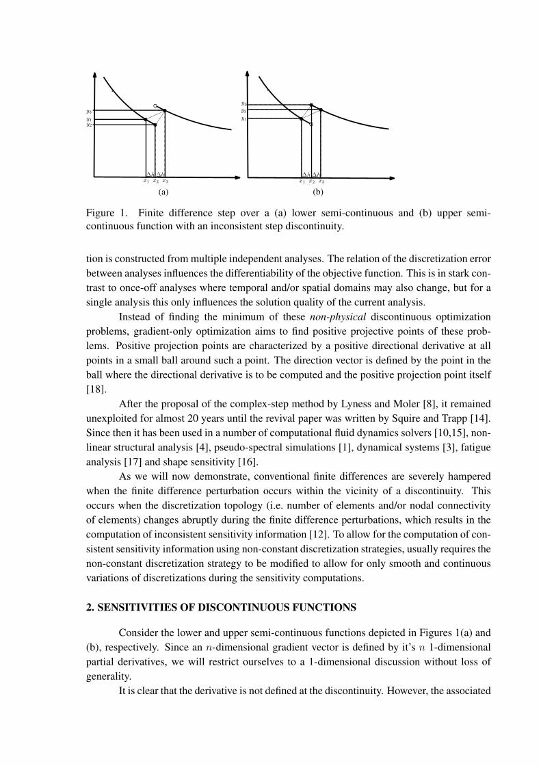
Figure 1. Finite difference step over a (a) lower semi-continuous and (b) upper semi-continuous function with an inconsistent step discontinuity.

tion is constructed from multiple independent analyses. The relation of the discretization errorbetween analyses influences the differentiability of the objective function. This is in stark con-trast to once-off analyses where temporal and/or spatial domains may also change, but for asingle analysis this only influences the solution quality of the current analysis.

Instead of finding the minimum of these non-physical discontinuous optimizationproblems, gradient-only optimization aims to find positive projective points of these prob-lems. Positive projection points are characterized by a positive directional derivative at allpoints in a small ball around such a point. The direction vector is defined by the point in theball where the directional derivative is to be computed and the positive projection point itself[18].

After the proposal of the complex-step method by Lyness and Moler [8], it remainedunexploited for almost 20 years until the revival paper was written by Squire and Trapp [14].Since then it has been used in a number of computational fluid dynamics solvers [10,15], non-linear structural analysis [4], pseudo-spectral simulations [1], dynamical systems [3], fatigueanalysis [17] and shape sensitivity [16].

As we will now demonstrate, conventional finite differences are severely hamperedwhen the finite difference perturbation occurs within the vicinity of a discontinuity. Thisoccurs when the discretization topology (i.e. number of elements and/or nodal connectivityof elements) changes abruptly during the finite difference perturbations, which results in thecomputation of inconsistent sensitivity information [12]. To allow for the computation of con-sistent sensitivity information using non-constant discretization strategies, usually requires thenon-constant discretization strategy to be modified to allow for only smooth and continuousvariations of discretizations during the sensitivity computations.

2. SENSITIVITIES OF DISCONTINUOUS FUNCTIONS

Consider the lower and upper semi-continuous functions depicted in Figures 1(a) and(b), respectively. Since an n-dimensional gradient vector is defined by it’s n 1-dimensionalpartial derivatives, we will restrict ourselves to a 1-dimensional discussion without loss ofgenerality.

It is clear that the derivative is not defined at the discontinuity. However, the associated

derivative [18] is defined everywhere and it is given by the left hand limit for lower semi-continuous functions and by the right hand limit for upper semi-continuous functions at thediscontinuity. The benefit of the complex-step derivative is that it computes the associatedderivative and allows the computation of sensitivity information even at a discontinuity. Aswe will consider in detail, the complex-step method achieves this by only taking an imaginarystep without the need to take a real step over the discontinuity.

In turn, conventional finite difference schemes requires a real step to be taken, withundesired consequences. Consider the following finite difference computations on the lowersemicontinuous function depicted Figure1 (a): forward (FD), backward (BD) and central dif-ference (CD) schemes computes the derivative as:(

dfdx

)FD

≈ y3−y2x3−x2

> 0,(dfdx

)BD

≈ y2−y1x2−x1

< 0,(dfdx

)CD

≈ y3−y1x3−x1

> 0,

(1)

whereas the upper semicontinuous function in Figure1 (b) results in the following:(dfdx

)FD

≈ y3−y2x3−x2

< 0,(dfdx

)BD

≈ y2−y1x2−x1

> 0,(dfdx

)CD

≈ y3−y1x3−x1

> 0.

(2)

It is clear that finite differences in the context of discontinuous functions are severely prob-lematic, with inconsistencies not only in the magnitude but also the direction (sign) of thecomputed sensitivities.

In contrast, the complex-step method avoids these problems. Consider the complexTaylor series expansion of an analytic function f(x) using a complex step i∆h,

f(x + i∆h) = f(x) + i∆hf ′(x)−∆h2f′′(x)

2+ higher order terms, (3)

By equating the imaginary parts of both sides of the equation, the complex-step derivativeapproximation Im[f(x+i∆h)]

∆his obtained as a second order accurate approximation to f ′(x).

The advantage of the complex-step method is that only a complex step i∆h on theimaginary axis is required, as opposed to a step along the real axis when using conventionalfinite differences. Hence, even at the discontinuity the derivative would be computed at thatpoint as if the function was smooth in the vicinity of that point. Therefore, derivative informa-tion can always be computed. Similarly, derivative information can also always be computedwhen using (semi)-analytical or automatic differentiation strategies. The computed sensitivi-ties are the associated derivative [18] that can be used for gradient-only optimization.

To demonstrate our arguments, consider the following simple piece-wise linear stepdiscontinuous function:

f(x) =

x < 1 : −2x− 0.5x ≥ 1 : −2x

. (4)

Mathematically, the derivative is not defined at x = 1. However, the associated derivative ofthis function is continuous and -2 everywhere, including at x = 1. Computing the derivativewith the complex step method yields exactly -2 everywhere, including x = 1, allowing a fullfield computation of the derivative of a discontinuous function.

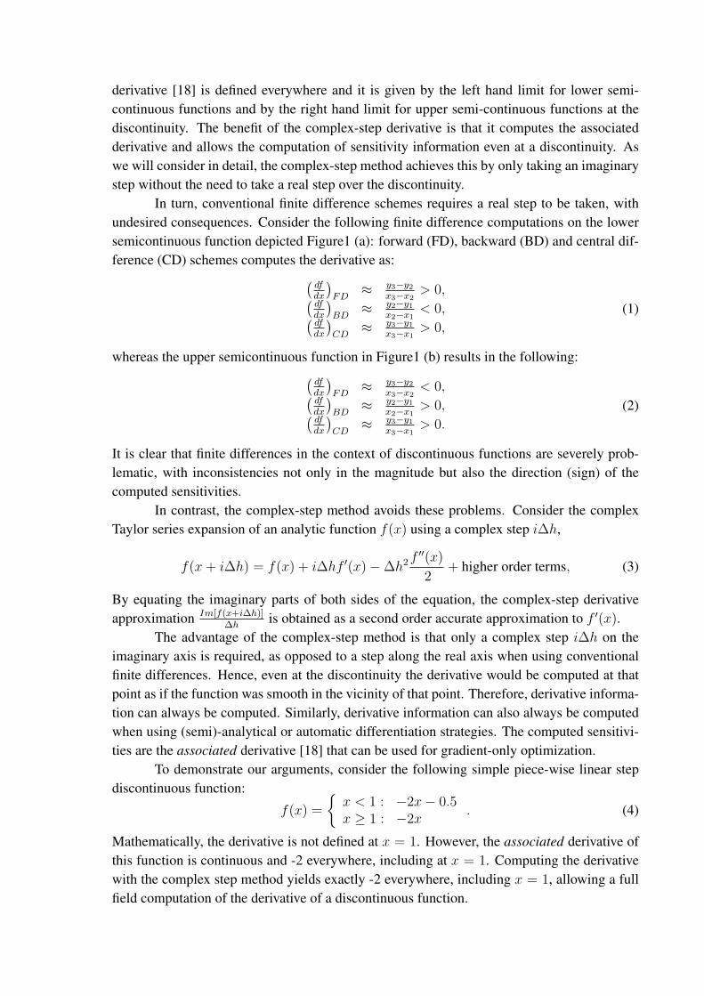
The truncation error is 0 for all finite difference schemes on each section of the piece-wise linear function. The choice for a piecewise linear function allows us to isolate the errordue to the discontinuity, and not be influenced by rounding errors.

Consider the results presented in Figure 2. The absolute round-off error as a functionof step size is presented in Figure 2 (a) for the linear function −2x, using forward, backwardand central difference schemes. The combined round-off and discontinuity error for the func-tion given in (4) is presented in Figure 2 (b). The derivative at x = 1 was approximatedusing the forward, backward and central difference schemes. The step sizes in both figuresare varied between 100 and 10−20. The results of the complex-step method is not presented asit exactly recovers a sensitivity of -2, everywhere.

10-20 10-18 10-16 10-14 10-12 10-10 10-8 10-6 10-4 10-2 100

step size ∆h

10-16

10-14

10-12

10-10

10-8

10-6

10-4

10-2

100

Absolute error of the computed sensitivity

forward differencebackward differencecentral difference

(a)

10-20 10-18 10-16 10-14 10-12 10-10 10-8 10-6 10-4 10-2 100

step size ∆h

10-16

10-13

10-10

10-7

10-4

10-1

102

105

108

1011

1014


forward differencebackward differencecentral difference

(b)

Figure 2. Finite difference computations for the (a) linear function f(x) = −2x and (b) linearfunction with discontinuity as given in (4).

The behaviour of the difference schemes corresponds to the anticipated behaviour asdescribed in (2). As expected the discontinuity error dominates and increases as the step sizeis reduced. It is easy to envisage a simple modification to finite difference schemes fromthe observation above that may be able to overcome the associated problems. For example,when the signs amongst the three computed derivatives differ, a simple modification may beto choose the derivative that is the most negative when considering minimization problems asgiven in (1) and (2). However, when considering multidimensional problems the discontinu-ities may not be isolated as is the case in Figure 1, with forward and backward steps occurringover different discontinuities.

Unfortunately, the complex-step method only allows for direct or forward mode com-putations of sensitivities. Hence, when dealing with a large number of design variables andonly a few functions the benefits of adjoint or reverse mode sensitivities cannot be exploited[11]. In addition, complex number calculations requires additional memory and computa-tional resources. Fortunately, modifications to programs mostly require only the accommoda-tion of complex variables, overloading a few functions and reviewing some branching state-ments. The authors found the guidelines presented by [9] more than adequate for all examplespresented in this paper.

3. SENSITIVITIES OF VARYING DISCRETIZATIONS

As pointed consistent sensitivity information needs to be computed when consideringobjective functions that rely on solutions of partial differential equations [12], which usuallyrequires a modification to non-constant discretization strategies to avoid any inconsistenciesduring the sensitivity computations.

As a practical example consider a linear elastic finite element based shape optimizationproblem, where the objective function F(x) is an explicit function of the nodal displacementsu. The nodal displacements u(Λ) in turn is a function of the discretization Λ (computationalmesh) defined on the domain Ω with boundary ∂Ω. The computational mesh

Λ ∈ X = (X i)i=1,...,nn;T = (T kj )j=1,...,ne;k=1,...,nv, (5)

describes the position X ∈ R3 of the nn nodes, and gives for each computational elementj = 1, . . . , ne the set T k=1,...,nv

j of its’ nv vertices [6]. For now we limit the nodal positionsto two dimensions X ∈ R2. The computational mesh Λ(x) in turn is a function of the designvariables x, which controls the discretized geometrical domain.

Following the usual finite element discretization of the linear elastic solid mechanicsboundary value problem we obtain

Ku = f , (6)

where K represents the assembled structural stiffness matrix and f the consistent structuralloads. The system in Eq. (6) is partitioned along the unknown displacements (uf) and theprescribed displacement (up), i.e.

Ku =

[K ff K fp

Kpf Kpp

]uf

up

=

f ff p

, (7)

where f f represents the prescribed forces and f p the reactions at the nodes with prescribeddisplacements. The unknown displacements (uf) are obtained from

K ffuf = f f −K fpup. (8)

Recall that the objective function F(x) is an explicit function of the nodal displace-ments u. Using gradient based optimisation algorithms, we therefore require the sensitivityof the structural response u w.r.t. the design variables (control variables) x. In general, thestiffness partition matrices K ff and K fp, the nodal displacement vector uf and the load vectorf f in Eq. (8) depend on the design variables x, i.e. K ff(x)uf(x) = f f(x)−K fp(x)up(x).

The analytical gradient dufdx

is obtained by differentiating Eq. (8) w.r.t. the control vari-ables x, i.e.

K ffduf

dx=

df f

dx−

dK fp

dxup −K fp

dup

dx− dK ff

dxuf. (9)

In this study the load vector f f is assumed to be independent of the control variables x, hencedf fdx

= 0. For Dirichlet boundary conditions, up = 0, and Eq. (9) reduces to

K ffduf

dx= −dK ff

dxuf. (10)

Eq. (10) is solved to obtain dufdx

, using the factored stiffness matrix K ff, available from theprimary analysis when solving Eq. (8). The unknown dKff

dxis computed from

dK ff

dx=

dK ff

dXdXdx

, (11)

where dKffdX is obtained by differentiating the stiffness matrix analytically with respect to the

nodal coordinates X . This is done on the element level and then assembled into the globalsystem.

To complete the sensitivity analysis, we still need to evaluate dXdx

present in Eq. (11).To compute consistent sensitivity information the current number of nodes nn and elementnodal connectivity T as defined in (5) needs to remain unchanged and any change in nodalpositions needs to be smooth and continuous [2,12]. In particular, when semi-analytical sen-sitivities are used to compute dX

dxusing conventional finite differences.

However, computing the sensitivity analytically yields consistent sensitivity informa-tion as no perturbation is required that may change the computational mesh Λ. Similarly, thebenefit of the complex-step method is that the computational mesh Λ remains unchanged onthe real axis as only a pure imaginary step is required to compute the sensitivity information.

Again, we highlight that accurate associated sensitivity information is computableeverywhere although the functions is not everywhere differentiable. This can be achieved byanalytical sensitivities, consistent semi-analytical sensitivities, automatic differentiation or thecomplex step method.

4. NUMERICAL EXPERIMENTS

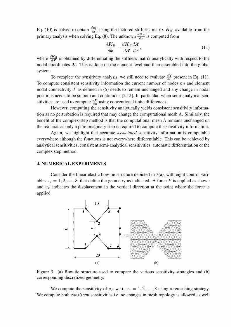
Consider the linear elastic bow-tie structure depicted in 3(a), with eight control vari-ables xi = 1, 2, . . . , 8, that define the geometry as indicated. A force F is applied as shownand uF indicates the displacement in the vertical direction at the point where the force isapplied.

(a) (b)

Figure 3. (a) Bow-tie structure used to compare the various sensitivity strategies and (b)corresponding discretized geometry.

We compute the sensitivity of uF w.r.t. xi = 1, 2, . . . , 8 using a remeshing strategy.We compute both consistent sensitivities i.e. no changes in mesh topology is allowed as well

as inconsistent sensitivities i.e. the mesh topology is allowed to change during the sensitivitycomputation.

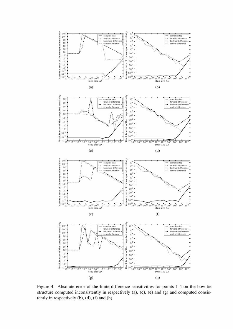
The absolute error for both the consistent and inconsistent sensitivity computationsfor the forward difference, backward difference, central difference and complex-step methodare depicted in Figures 4 and 5. The inconsistent sensitivities for points 1-4 are depicted inFigures 4 (a), (c), (e) and (g) respectively, while the absolute sensitivity error for points 5-8are depicted in Figures 5 (a), (c), (e) and (g). In turn, the absolute error for the consistentsensitivities are depicted in Figures 4 (b), (d), (f) and (h) and in Figures 5 (b), (d), (f) and (h)for respectively points 1-4 and 5-8 respectively.

Note that the absolute error of the complex-step sensitivities are unaffected whetherthe non-constant discretization strategy preserves the mesh topology or not. This is in starkcontrast to the finite difference strategies who’s absolute error severely degrades for incon-sistent sensitivities as opposed to consistent sensitivities. Consider the inconsistent sensitiv-ity computation of point 3, as depicted in Figure 4(e). It is clear that neither the forward,backward, or central difference schemes compute appropriate sensitivities and hence even amodified difference strategy as discussed in Section 2 would fail to give accurate sensitivities,independent of the step size.

Consider the absolute error of the backward difference computed sensitivity error de-picted in Figure 5(e). As indicated, a jump in the absolute error of the sensitivity occurs fora step size change from 10−8 to 10−9, with the latter significantly more accurate. The jumpin error is a result of a change in the mesh topology from being inconsistent for the 10−8 stepsize to being consistent for the 10−9 step size. This is clearly depicted in Figure 6, wherethe initial mesh (in dashed lines) is superimposed onto the finite difference perturbed meshfor step sizes 10−8 and 10−9 respectively in Figures 6(a) and (b). Changes in the perturbedmesh is evident in the lower left part of the bow-tie structure. Although these changes in meshtopology are removed from point 7 where the sensitivity is computed as well as the pointwhere the load is applied, the discretization error in the stiffness of the structure is significantenough to adversely affect sensitivity computations.

5. CONCLUSION

We demonstrated the benefits of the complex-step method to compute accurate sen-sitivity information for discontinuous functions. The complex-step method allows for thecomputation of sensitivity information at a discontinuity where the derivative is not defined.We showed that the complex-step method is a viable numerical strategy to compute associatedderivatives or associated gradients, as required by gradient-only optimization.

We highlighted the well known need for consistent sensitivity computations when us-ing non-constant discretization strategies during objective or constraint computations. Thecomplex-step method allows for the computation of consistent sensitivity information withsimilar ease as for conventional finite differences, without having to modify non-constant dis-cretization strategies to preserve discretization topology during sensitivity calculations. Onlyminor modifications are required, which include the handling of complex variables, the over-loading of some functions and reviewing some branching statements.

10-20 10-18 10-16 10-14 10-12 10-10 10-8 10-6 10-4 10-2

step size ∆h

10-1510-1310-1110-910-710-510-310-110110310510710910111013


complex stepforward differencebackward differencecentral difference

(a)

10-20 10-18 10-16 10-14 10-12 10-10 10-8 10-6 10-4 10-2

step size ∆h

10-1310-1110-910-710-510-310-1101103105107109



(b)

10-20 10-18 10-16 10-14 10-12 10-10 10-8 10-6 10-4 10-2

step size ∆h

10-1410-1210-1010-810-610-410-2100102104106108



(c)

10-20 10-18 10-16 10-14 10-12 10-10 10-8 10-6 10-4 10-2

step size ∆h

10-13

10-11

10-9

10-7

10-5

10-3

10-1

101

103

105

107



(d)

10-20 10-18 10-16 10-14 10-12 10-10 10-8 10-6 10-4 10-2

step size ∆h

10-1310-1110-910-710-510-310-110110310510710910111013



(e)

10-20 10-18 10-16 10-14 10-12 10-10 10-8 10-6 10-4 10-2

step size ∆h

10-1310-1110-910-710-510-310-1101103105107109



(f)

10-20 10-18 10-16 10-14 10-12 10-10 10-8 10-6 10-4 10-2

step size ∆h

10-1010-810-610-410-2100102104106108101010121014



(g)

10-20 10-18 10-16 10-14 10-12 10-10 10-8 10-6 10-4 10-2

step size ∆h

10-10

10-8

10-6

10-4

10-2

100

102

104

106

108

1010



(h)

Figure 4. Absolute error of the finite difference sensitivities for points 1-4 on the bow-tiestructure computed inconsistently in respectively (a), (c), (e) and (g) and computed consis-tently in respectively (b), (d), (f) and (h).

10-20 10-18 10-16 10-14 10-12 10-10 10-8 10-6 10-4 10-2

step size ∆h

10-14

10-11

10-8

10-5

10-2

101

104

107

1010

1013

1016



(a)

10-20 10-18 10-16 10-14 10-12 10-10 10-8 10-6 10-4 10-2

step size ∆h

10-1310-1110-910-710-510-310-1101103105107109



(b)

10-20 10-18 10-16 10-14 10-12 10-10 10-8 10-6 10-4 10-2

step size ∆h

10-14

10-12

10-10

10-8

10-6

10-4

10-2

100

102



(c)

10-20 10-18 10-16 10-14 10-12 10-10 10-8 10-6 10-4 10-2

step size ∆h

10-1410-1210-1010-810-610-410-2100102104106108



(d)

(e)

10-20 10-18 10-16 10-14 10-12 10-10 10-8 10-6 10-4 10-2

step size ∆h

10-1210-1010-810-610-410-21001021041061081010



(f)

10-20 10-18 10-16 10-14 10-12 10-10 10-8 10-6 10-4 10-2

step size ∆h

10-1110-910-710-510-310-11011031051071091011



(g)

10-20 10-18 10-16 10-14 10-12 10-10 10-8 10-6 10-4 10-2

step size ∆h

10-1110-910-710-510-310-11011031051071091011



(h)

Figure 5. Absolute error of the finite difference sensitivities for points 5-8 on the bow-tiestructure computed inconsistently in respectively (a), (c), (e) and (g) and computed consis-tently in respectively (b), (d), (f) and (h).

0 2 4 6 8 10 12 14 16 18 200

5

10

15

(a)0 2 4 6 8 10 12 14 16 18 20

0

5

10

15

(b)

Figure 6. Consider the inconsistent backward difference sensitivity computation of point 7with absolute error depicted in Figure 5(e). Depicted are the initial mesh (dashed line) super-imposed onto the backward difference mesh (solid line) with step sizes of (a) 10−8 and (b)10−9, respectively. The change is mesh topology is evident in the lower left of (a) as opposedto no change in mesh topology in (b).

6. REFERENCES

[1] Cervino L., Bewley T., “On the extension of the complex-step derivative technique topseudospectral algorithms”. J. Comput. Phys. 187, 544-549, 2003.

[2] van Keulen F., Haftka R., Kim N., “Review of options for structural design sensitivityanalysis Part 1 : Linear systems”. Comput. Method. Appl. M. 194, 3213-3243, 2005.

[3] Kim J., Bates D., Postlethwaite I., “Nonlinear robust performance analysis usingcomplex-step gradient approximation”. Automatica 42, 177-182, 2006.

[4] Kim S., Ryu J., Cho M., “Numerically generated tangent stiffness matrices using thecomplex variable derivative method for nonlinear structural analysiss”. Comput. Method.Appl. M. 200, 403-413, 2011.

[5] Lai K.L., Crassidis J., ‘Generalizations of the complex-step derivative approximation”.Coll. Tech. Papers: AIAA Guid. Nav. Contrl. Conf. 4, 2540-2564, 2006.

[6] Laporte E., Tallec P.L., Numerical Methods in Sensitivity Analysis and Shape Optimiza-tion. Modeling and Simulation in Science, Birkhauser, 2002.

[7] Lyness J., “Differentiation formulas for analytic functions”. Math. Comput. 22, 352-362,1968.

[8] Lyness J., Moler C., “Numerical Differentiation of Analytic Functions”. SIAM J. Numer.Anal. 4, 202-210,1967.

[9] Martins J., Sturdza P., Alonso J.J., “The Complex-Step Derivative Approximation”. ACMT. Math. Software 29, 245-262, 2003.

[10] Martins J., Alonso J., Reuther J., “A Coupled-Adjoint Sensitivity Analysis Method forHigh-Fidelity Aero-Structural Design”. Optim. Eng. 6, 33-62, 2005.

[11] Martins J.R.R.A., Sturdza P., Alonso J.J., “The connection between the complex-stepderivative approximation and algorithmic differentiation”. AIAA Paper 921, 1-11, 2001.

[12] Schleupen A., Maute K., Ramm E., “Adaptive FE-procedures in shape optimization”.Struct. Multidiscip. O. 19, 282-302, 2000.

[13] Shor N., “New development trends in nondifferentiable optimization”. Cybern. Syst.Anal+ 13, 881-886, 1977.

[14] Squire M., Trapp G., “Using Complex Variables to estimate derivatives of real functions”.SIAM Rev. 40, 110-112, 1998.

[15] Vatsa V., “Computation of sensitivity derivatives of Navier-Stokes equations using com-plex variables”. Adv. Eng. Softw. 31, 655-659, 2000.

[16] Voorhees A., Millwater H., Bagley R., “Complex variable methods for shape sensitivityof finite element methods”. Finite Elem. Anal. Des. 47, 1146-1156, 2011.

[17] Voorhees A., Millwater H., Bagley R., Golden P., “Fatigue sensitivity analysis using com-plex variable methods”. Int. J. Fatigue 40, 61-73, 2012.

[18] Wilke D.N., Kok S., Snyman J.A., Groenwold A.A., “Gradient-only approaches to avoidspurious local minima in unconstrained optimization”. Opt. Eng. available online, 2012.

NUMERICAL SENSITIVITY COMPUTATION FOR DISCONTINUOUS...

Documents

Transcript of NUMERICAL SENSITIVITY COMPUTATION FOR DISCONTINUOUS...