Numerical Schemes for Advection Reaction Equation Ramaz Botchorishvili Faculty of Exact and Natural...
44
Numerical Schemes for Advection Reaction Equation Ramaz Botchorishvili Faculty of Exact and Natural Sciences Tbilisi State University GGSWBS,Tbilisi, July 07-11, 2014 1
-
Upload
tobias-williamson -
Category
Documents
-
view
218 -
download
0
Transcript of Numerical Schemes for Advection Reaction Equation Ramaz Botchorishvili Faculty of Exact and Natural...

1
Numerical Schemes for Advection Reaction Equation
Ramaz Botchorishvili
Faculty of Exact and Natural Sciences
Tbilisi State University
GGSWBS,Tbilisi, July 07-11, 2014

2
Outline Equations Operator splitting Baricentric interpolation and derivative Simple high order schemes Divided differences Stable high order scheme Multischeme Discretization for ODEs

3
Equation
)()(),(),0( 00 BVLuxuxu
),()(
tufx
vu
t
u
v(t,x) - velocityf (u,t) – reaction smooth functions

4
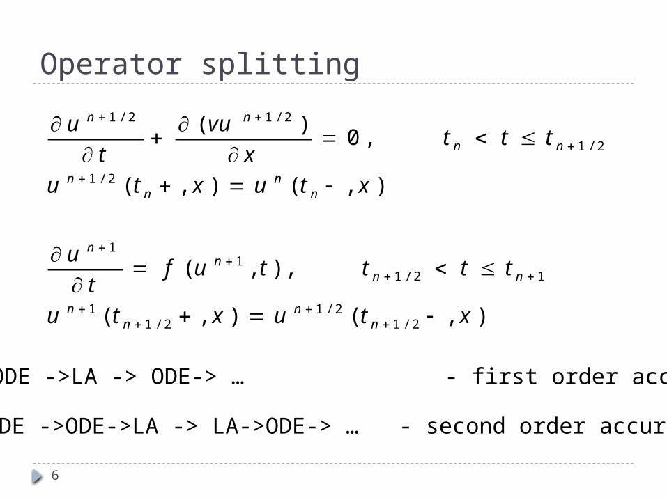
Operator splitting
),(),(
),,(
),(),(
,0)(
2/12/1
2/11
12/11
1
2/1
2/1
2/12/1
xtuxtu
ttttuft
u
xtuxtu
tttx
vu
t
u
nn
nn
nnn
n
nn
nn
nn
nn

5
Operator splitting
),(),(
),,(
),(),(
,0)(
2/12/1
2/11
12/11
1
2/1
2/1
2/12/1
xtuxtu
ttttuft
u
xtuxtu
tttx
vu
t
u
nn
nn
nnn
n
nn
nn
nn
nn
LA -> ODE ->LA -> ODE-> … - first order accurate
6
Operator splitting
),(),(
),,(
),(),(
,0)(
2/12/1
2/11
12/11
1
2/1
2/1
2/12/1
xtuxtu
ttttuft
u
xtuxtu
tttx
vu
t
u
nn
nn
nnn
n
nn
nn
nn
nn
LA -> ODE ->LA -> ODE-> … - first order accurate
LA -> ODE ->ODE->LA -> LA->ODE-> … - second order accurate

7
Interpolation
bxxxa n 10
nyyy ,,, 10
)(,),(0 xx n
n
iii xax
0
)()(
niyx ii ,,1,0,)(

8
Lagrange interpolation
n
iniin xlyxL
0, )()(
nixx
xx
xxxxxxxx
xxxxxxxxxl
n
ijj
ji
n
ijj
j
niiiiii
niini ,0,
)(
)(
)())(()(
)())(()()(
0
0
110
110,
n
jkjkj
n
jkjnikn nkyyxlyxL
00, 0,)()(

9
Lagrange interpolation
n
iniin xlyxL
0, )()(
nixx
xx
xxxxxxxx
xxxxxxxxxl
n
ijj
ji
n
ijj
j
niiiiii
niini ,0,
)(
)(
)())(()(
)())(()()(
0
0
110
110,
n
jkjkj
n
jkjnikn nkyyxlyxL
00, 0,)()(
Pros & cons

10
Barycentric interpolation
n
i i
iinn xxyxxL
0
)()(
n
jjn xxx
0
)()(
n
ijj
ji
ii
in
n
ijj
ji
n
ijj
j
niiiiii
niini
xxni
xxx
xx
xx
xxxxxxxx
xxxxxxxxxl
0
0
0
110
110,
)(
1,,0,)(
)(
)(
)())(()(
)())(()()(

11
Barycentric interpolation
n
i i
iinn xxyxxL
0
)()(
n
jjn xxx
0
)()(
n
ijj
ji
i
xx0
)(
1
12
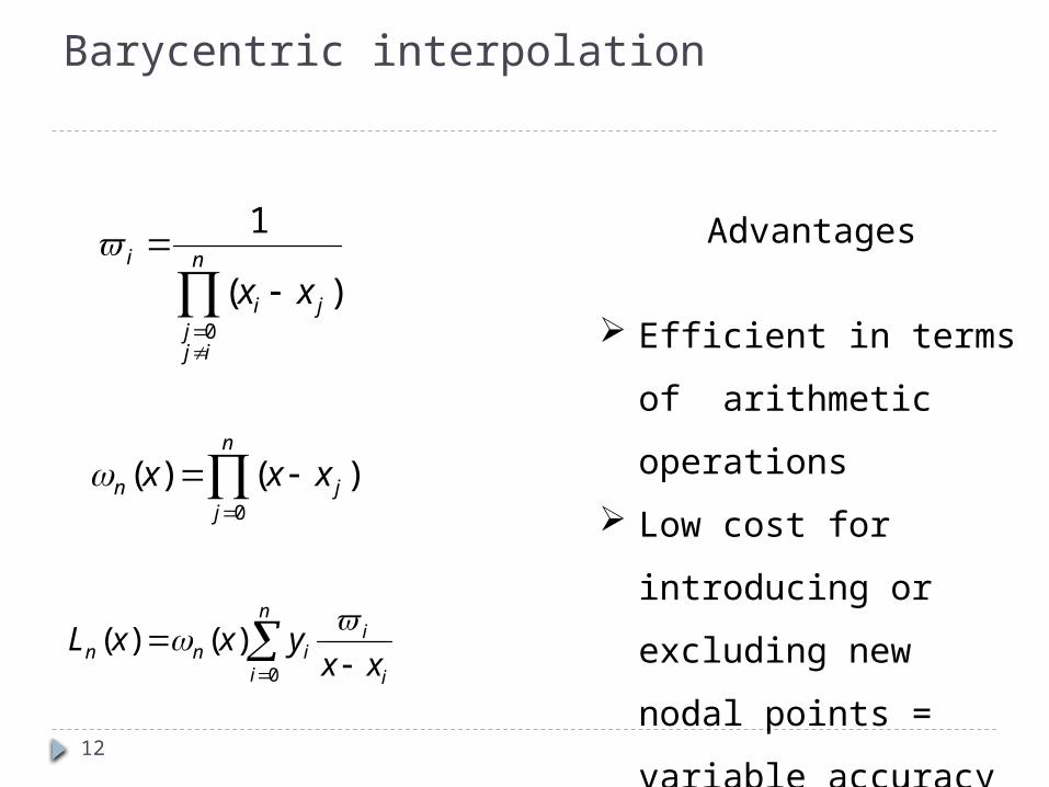
Barycentric interpolation
Advantages
Efficient in terms of
arithmetic operations
Low cost for
introducing or
excluding new nodal
points = variable
accuracy
n
i i
iinn xxyxxL
0
)()(
n
jjn xxx
0
)()(
n
ijj
ji
i
xx0
)(
1

13
Baricentric derivative

14
Baricentric derivative
Advantages:
Easy for
implementing
Arithmetic
operations
High order accuracy

15
High order scheme for LA
n
nii in
nnniii
nnn xx
uvuvxL
2
,02
)()(1)(
n
ijj
ji
i
xx2
0
)(
1
x
vu
)(
Approximation for
N=1, 2nd orderN=2, 4th orderN=4 , 8th order…

16
High order scheme for LA
0)()(1 2
,0
1
n
nii in
kn
knn
ki
kii
n
kn
kn
xx
uvuvuu
n
ijj
ji
i
xx2
0
)(
1
First order accurate in time, 2n order accurate in space

17
High order scheme for LA
0)()(1 2
,0
1
n
nii in
kn
knn
ki
kii
n
kn
kn
xx
uvuvuu
n
ijj
ji
i
xx2
0
)(
1
First order accurate in time, 2n order accurate in space
Possible Problems conservation & stability

18
Firs order upwind
0])()[(])()[( 1111
1
h
uvuvuvuvuu ki
ki
ki
ki
ki
ki
ki
ki
ki
ki

19
Firs order upwind
0])()[(])()[( 1111
1
h
uvuvuvuvuu ki
ki
ki
ki
ki
ki
ki
ki
ki
ki
Numerical flux functions

20
Firs order upwind
0])()[(])()[( 1111
1
h
uvuvuvuvuu ki
ki
ki
ki
ki
ki
ki
ki
ki
ki
Numerical flux functions
Properties1. Consistency2. Conditional stability (CFL)3. First order in space and in time4. conservative

21
Firs order upwind
0])()[(])()[( 1111
1
h
uvuvuvuvuu ki
ki
ki
ki
ki
ki
ki
ki
ki
ki
Numerical flux functions
Properties1. Consistency2. Conditional stability (CFL)3. First order in space and in time4. conservative
ki
ki
ki vvv )()(
1|))(||)(|max ki
ki vv
h
i
ki
i
ki uu 1

22
High order conservative discretisation
0])()[(])()[( 1111
1
h
uvuvuvuvuu ki
ki
ki
ki
ki
ki
ki
ki
ki
ki
02/12/11
h
FFuu iiki
ki

23
High order conservative discretisation
0])()[(])()[( 1111
1
h
uvuvuvuvuu ki
ki
ki
ki
ki
ki
ki
ki
ki
ki
02/12/11
h
FFuu iiki
ki
Harten, Enquist, Osher, Chakravarthy:
given function in values in nodal points, how to interpolate at cell interfaces in order to get higher then 2 accuracy

24
Special interpolation/reconstruction procedure
g(x)= 𝑓ሺ𝑦ሻ𝑑𝑦𝑥−∞
g(𝑥𝑖+1 2Τ )=σ 𝑓ሺ𝑦ሻ𝑑𝑦𝑥𝑖+1 2Τ𝑥𝑖−1 2Τ𝑖𝑗=−∞ =σ 𝑓ҧ𝑗∆𝑥𝑗𝑖𝑗=−∞
𝑓ҧ𝑗 = 1∆𝑥𝑗න 𝑓ሺ𝑦ሻ𝑑𝑦𝑥𝑗+1 2Τ𝑥𝑗−1 2Τ
P(x)-interpolation polinomial using g(𝑥𝑖+1 2Τ )
p(x)=P’(x)-derivative

25
Special interpolation/reconstruction procedure
g(x)= 𝑓ሺ𝑦ሻ𝑑𝑦𝑥−∞
g(𝑥𝑖+1 2Τ )=σ 𝑓ሺ𝑦ሻ𝑑𝑦𝑥𝑖+1 2Τ𝑥𝑖−1 2Τ𝑖𝑗=−∞ =σ 𝑓ҧ𝑗∆𝑥𝑗𝑖𝑗=−∞
𝑓ҧ𝑗 = 1∆𝑥𝑗න 𝑓ሺ𝑦ሻ𝑑𝑦𝑥𝑗+1 2Τ𝑥𝑗−1 2Τ
P(x)-interpolation polinomial using g(𝑥𝑖+1 2Τ )
p(x)=P’(x)-derivative

26
Special interpolation/reconstruction procedure
g(x)= 𝑓ሺ𝑦ሻ𝑑𝑦𝑥−∞
g(𝑥𝑖+1 2Τ )=σ 𝑓ሺ𝑦ሻ𝑑𝑦𝑥𝑖+1 2Τ𝑥𝑖−1 2Τ𝑖𝑗=−∞ =σ 𝑓ҧ𝑗∆𝑥𝑗𝑖𝑗=−∞
𝑓ҧ𝑗 = 1∆𝑥𝑗න 𝑓ሺ𝑦ሻ𝑑𝑦𝑥𝑗+1 2Τ𝑥𝑗−1 2Τ
P(x)-interpolation polinomial using g(𝑥𝑖+1 2Τ )
p(x)=P’(x)-derivative

27
Special interpolation/reconstruction procedure
g(x)= 𝑓ሺ𝑦ሻ𝑑𝑦𝑥−∞
g(𝑥𝑖+1 2Τ )=σ 𝑓ሺ𝑦ሻ𝑑𝑦𝑥𝑖+1 2Τ𝑥𝑖−1 2Τ𝑖𝑗=−∞ =σ 𝑓ҧ𝑗∆𝑥𝑗𝑖𝑗=−∞
𝑓ҧ𝑗 = 1∆𝑥𝑗න 𝑓ሺ𝑦ሻ𝑑𝑦𝑥𝑗+1 2Τ𝑥𝑗−1 2Τ
P(x)-interpolation polinomial using g(𝑥𝑖+1 2Τ )
p(x)=P’(x)-derivative

28
Special interpolation/reconstruction procedure
1∆𝑥𝑗 𝑝ሺ𝑥ሻ𝑑𝑥𝑥𝑗+1 2Τ𝑥𝑗−1 2Τ = 1∆𝑥𝑗 (g(𝑥𝑖+1 2Τ )- g(𝑥𝑖−1 2Τ ))= 1∆𝑥𝑗 𝑓ሺ𝑦ሻ𝑑𝑦𝑥𝑗+1 2Τ𝑥𝑗−1 2Τ =𝑓ҧ𝑗
P’(x)=g(x)+o(∆𝑥𝑘) p(x)=f(x)+ o(∆𝑥𝑘)
P(x)=σ 𝑔(𝑥𝑖−𝑟+𝑚−1 2ൗ�𝑘𝑚=0 )𝑙𝑚(𝑥)
P(x)- 𝑔(𝑥𝑖−𝑟−1 2ൗ�)=σ ቈ𝑔ቆ𝑥𝑖−𝑟−𝑚−1 2ൗ�ቇ− 𝑔(𝑥𝑖−𝑟−1 2ൗ�)𝑘𝑚=0 𝑙𝑚(𝑥)
𝑔(𝑥𝑖−𝑟+𝑚−1 2ൗ�) − 𝑔(𝑥𝑖−𝑟−1 2ൗ�)=σ 𝑔ҧ𝑖−𝑟+𝑗𝑚−1𝑗=0 ∆𝑥𝑖−𝑟+𝑗

29
Special interpolation/reconstruction procedure
1∆𝑥𝑗 𝑝ሺ𝑥ሻ𝑑𝑥𝑥𝑗+1 2Τ𝑥𝑗−1 2Τ = 1∆𝑥𝑗 (g(𝑥𝑖+1 2Τ )- g(𝑥𝑖−1 2Τ ))= 1∆𝑥𝑗 𝑓ሺ𝑦ሻ𝑑𝑦𝑥𝑗+1 2Τ𝑥𝑗−1 2Τ =𝑓ҧ𝑗
P’(x)=g(x)+o(∆𝑥𝑘) p(x)=f(x)+ o(∆𝑥𝑘)
P(x)=σ 𝑔(𝑥𝑖−𝑟+𝑚−1 2ൗ�𝑘𝑚=0 )𝑙𝑚(𝑥)
P(x)- 𝑔(𝑥𝑖−𝑟−1 2ൗ�)=σ ቈ𝑔ቆ𝑥𝑖−𝑟−𝑚−1 2ൗ�ቇ− 𝑔(𝑥𝑖−𝑟−1 2ൗ�)𝑘𝑚=0 𝑙𝑚(𝑥)
𝑔(𝑥𝑖−𝑟+𝑚−1 2ൗ�) − 𝑔(𝑥𝑖−𝑟−1 2ൗ�)=σ 𝑔ҧ𝑖−𝑟+𝑗𝑚−1𝑗=0 ∆𝑥𝑖−𝑟+𝑗

30
Special interpolation/reconstruction procedure
1∆𝑥𝑗 𝑝ሺ𝑥ሻ𝑑𝑥𝑥𝑗+1 2Τ𝑥𝑗−1 2Τ = 1∆𝑥𝑗 (g(𝑥𝑖+1 2Τ )- g(𝑥𝑖−1 2Τ ))= 1∆𝑥𝑗 𝑓ሺ𝑦ሻ𝑑𝑦𝑥𝑗+1 2Τ𝑥𝑗−1 2Τ =𝑓ҧ𝑗
P’(x)=g(x)+o(∆𝑥𝑘) p(x)=f(x)+ o(∆𝑥𝑘)
P(x)=σ 𝑔(𝑥𝑖−𝑟+𝑚−1 2ൗ�𝑘𝑚=0 )𝑙𝑚(𝑥)
P(x)- 𝑔(𝑥𝑖−𝑟−1 2ൗ�)=σ ቈ𝑔ቆ𝑥𝑖−𝑟−𝑚−1 2ൗ�ቇ− 𝑔(𝑥𝑖−𝑟−1 2ൗ�)𝑘𝑚=0 𝑙𝑚(𝑥)
𝑔(𝑥𝑖−𝑟+𝑚−1 2ൗ�) − 𝑔(𝑥𝑖−𝑟−1 2ൗ�)=σ 𝑔ҧ𝑖−𝑟+𝑗𝑚−1𝑗=0 ∆𝑥𝑖−𝑟+𝑗

31
Special interpolation/reconstruction procedure
1∆𝑥𝑗 𝑝ሺ𝑥ሻ𝑑𝑥𝑥𝑗+1 2Τ𝑥𝑗−1 2Τ = 1∆𝑥𝑗 (g(𝑥𝑖+1 2Τ )- g(𝑥𝑖−1 2Τ ))= 1∆𝑥𝑗 𝑓ሺ𝑦ሻ𝑑𝑦𝑥𝑗+1 2Τ𝑥𝑗−1 2Τ =𝑓ҧ𝑗
P’(x)=g(x)+o(∆𝑥𝑘) p(x)=f(x)+ o(∆𝑥𝑘)
P(x)=σ 𝑔(𝑥𝑖−𝑟+𝑚−1 2ൗ�𝑘𝑚=0 )𝑙𝑚(𝑥)
P(x)- 𝑔(𝑥𝑖−𝑟−1 2ൗ�)=σ ቈ𝑔ቆ𝑥𝑖−𝑟−𝑚−1 2ൗ�ቇ− 𝑔(𝑥𝑖−𝑟−1 2ൗ�)𝑘𝑚=0 𝑙𝑚(𝑥)
𝑔(𝑥𝑖−𝑟+𝑚−1 2ൗ�) − 𝑔(𝑥𝑖−𝑟−1 2ൗ�)=σ 𝑔ҧ𝑖−𝑟+𝑗𝑚−1𝑗=0 ∆𝑥𝑖−𝑟+𝑗

32
Special interpolation/reconstruction procedure
1∆𝑥𝑗 𝑝ሺ𝑥ሻ𝑑𝑥𝑥𝑗+1 2Τ𝑥𝑗−1 2Τ = 1∆𝑥𝑗 (g(𝑥𝑖+1 2Τ )- g(𝑥𝑖−1 2Τ ))= 1∆𝑥𝑗 𝑓ሺ𝑦ሻ𝑑𝑦𝑥𝑗+1 2Τ𝑥𝑗−1 2Τ =𝑓ҧ𝑗
P’(x)=g(x)+o(∆𝑥𝑘) p(x)=f(x)+ o(∆𝑥𝑘)
P(x)=σ 𝑔(𝑥𝑖−𝑟+𝑚−1 2ൗ�𝑘𝑚=0 )𝑙𝑚(𝑥)
P(x)- 𝑔(𝑥𝑖−𝑟−1 2ൗ�)=σ ቈ𝑔ቆ𝑥𝑖−𝑟−𝑚−1 2ൗ�ቇ− 𝑔(𝑥𝑖−𝑟−1 2ൗ�)𝑘𝑚=0 𝑙𝑚(𝑥)
𝑔(𝑥𝑖−𝑟+𝑚−1 2ൗ�) − 𝑔(𝑥𝑖−𝑟−1 2ൗ�)=σ 𝑔ҧ𝑖−𝑟+𝑗𝑚−1𝑗=0 ∆𝑥𝑖−𝑟+𝑗

33
Special interpolation/reconstruction procedure
ቀP(x) − 𝑔(𝑥𝑖−𝑟−1 2ൗ�)ቁ′=p(x)
𝑓𝑗+1 2Τ = 𝑓ቀ𝑥𝑗+1 2ൗ�ቁ= 𝑝ቀ𝑥𝑗+1 2ൗ�ቁ= ൬𝑃ሺ𝑥ሻ− 𝑔ቀ𝑥𝑖−𝑟−1 2ൗ�ቁ൰ቚ𝑥=𝑥𝑗+1 2ൗ�′
Baricentric derivative?
1∆𝑥𝑖 𝜕𝑓𝜕𝑥 𝑑𝑥𝑥𝑖+1 2Τ𝑥𝑖−1 2Τ = 1∆𝑥𝑖 (𝑓𝑖+1 2Τ − 𝑓𝑖−1 2Τ )

34
Special interpolation/reconstruction procedure
ቀP(x) − 𝑔(𝑥𝑖−𝑟−1 2ൗ�)ቁ′=p(x)
𝑓𝑗+1 2Τ = 𝑓ቀ𝑥𝑗+1 2ൗ�ቁ= 𝑝ቀ𝑥𝑗+1 2ൗ�ቁ= ൬𝑃ሺ𝑥ሻ− 𝑔ቀ𝑥𝑖−𝑟−1 2ൗ�ቁ൰ቚ𝑥=𝑥𝑗+1 2ൗ�′
Baricentric derivative?
1∆𝑥𝑖 𝜕𝑓𝜕𝑥 𝑑𝑥𝑥𝑖+1 2Τ𝑥𝑖−1 2Τ = 1∆𝑥𝑖 (𝑓𝑖+1 2Τ − 𝑓𝑖−1 2Τ )

35
Special interpolation/reconstruction procedure
ቀP(x) − 𝑔(𝑥𝑖−𝑟−1 2ൗ�)ቁ′=p(x)
𝑓𝑗+1 2Τ = 𝑓ቀ𝑥𝑗+1 2ൗ�ቁ= 𝑝ቀ𝑥𝑗+1 2ൗ�ቁ= ൬𝑃ሺ𝑥ሻ− 𝑔ቀ𝑥𝑖−𝑟−1 2ൗ�ቁ൰ቚ𝑥=𝑥𝑗+1 2ൗ�′
Baricentric derivative?
1∆𝑥𝑖 𝜕𝑓𝜕𝑥 𝑑𝑥𝑥𝑖+1 2Τ𝑥𝑖−1 2Τ = 1∆𝑥𝑖 (𝑓𝑖+1 2Τ − 𝑓𝑖−1 2Τ )
36
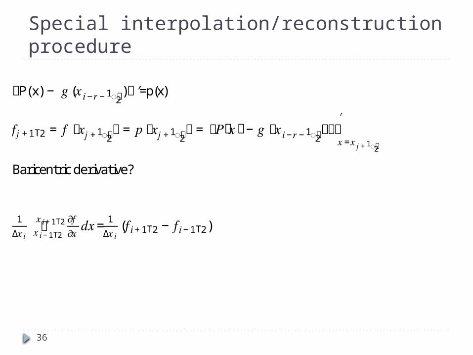
Special interpolation/reconstruction procedure
ቀP(x) − 𝑔(𝑥𝑖−𝑟−1 2ൗ�)ቁ′=p(x)
𝑓𝑗+1 2Τ = 𝑓ቀ𝑥𝑗+1 2ൗ�ቁ= 𝑝ቀ𝑥𝑗+1 2ൗ�ቁ= ൬𝑃ሺ𝑥ሻ− 𝑔ቀ𝑥𝑖−𝑟−1 2ൗ�ቁ൰ቚ𝑥=𝑥𝑗+1 2ൗ�′
Baricentric derivative?
1∆𝑥𝑖 𝜕𝑓𝜕𝑥 𝑑𝑥𝑥𝑖+1 2Τ𝑥𝑖−1 2Τ = 1∆𝑥𝑖 (𝑓𝑖+1 2Τ − 𝑓𝑖−1 2Τ )

37
Special interpolation/reconstruction procedure
ቀP(x) − 𝑔(𝑥𝑖−𝑟−1 2ൗ�)ቁ′=p(x)
𝑓𝑗+1 2Τ = 𝑓ቀ𝑥𝑗+1 2ൗ�ቁ= 𝑝ቀ𝑥𝑗+1 2ൗ�ቁ= ൬𝑃ሺ𝑥ሻ− 𝑔ቀ𝑥𝑖−𝑟−1 2ൗ�ቁ൰ቚ𝑥=𝑥𝑗+1 2ൗ�′
Baricentric derivative?
1∆𝑥𝑖 𝜕𝑓𝜕𝑥 𝑑𝑥𝑥𝑖+1 2Τ𝑥𝑖−1 2Τ = 1∆𝑥𝑖 (𝑓𝑖+1 2Τ − 𝑓𝑖−1 2Τ )
02/12/11
h
FFuu iiki
ki
High order accurate approximation

38
Special interpolation/reconstruction procedure
ቀP(x) − 𝑔(𝑥𝑖−𝑟−1 2ൗ�)ቁ′=p(x)
𝑓𝑗+1 2Τ = 𝑓ቀ𝑥𝑗+1 2ൗ�ቁ= 𝑝ቀ𝑥𝑗+1 2ൗ�ቁ= ൬𝑃ሺ𝑥ሻ− 𝑔ቀ𝑥𝑖−𝑟−1 2ൗ�ቁ൰ቚ𝑥=𝑥𝑗+1 2ൗ�′
Baricentric derivative?
1∆𝑥𝑖 𝜕𝑓𝜕𝑥 𝑑𝑥𝑥𝑖+1 2Τ𝑥𝑖−1 2Τ = 1∆𝑥𝑖 (𝑓𝑖+1 2Τ − 𝑓𝑖−1 2Τ )
02/12/11
h
FFuu iiki
ki
High order accurate approximation

39
Components of high order scheme
Discretization of the divergence operator • baricentric interpolation • baricentric derivative• ENO type reconstruction procedure (Harten, Enquist, Osher, Chakravarthy): • Given fluxes in nodal points• Interpolate fluxes at cell interfaces in such a way
that central finite difference formula provides high order (higher then 2) approximation
• Use adaptive stencils to avoid oscillations

40
Adaptation of interpolation
Use adaptive stencils to avoid oscillations•interpolate with high order polynomial in all cell interfaces inside of the stencil of the polynomial•If local maximum principle is satisfied then value at this cell interface is found•If local maximum principle is not satisfied then change stencil and repeat interpolation procedure for such cell interfaces•If after above procedure local maximum principle is not respected then reduce order of polynomial and repeat procedure for those interfaces only

41
Convergence in one space dimension Algorithm ensures
Uniform bound of approximate solutions Uniform bound of total variation
ConclusionsApproximate solution converge a.e. to solution of the original problem

42
Extension to higher spatial dimension Cartesian meshes:
strightforward Hexagonal meshes:
Directional derivates => div needs three directional derivatives in 2D
Implementation with baricentric derivatives without adaptation procedure See poster ( Tako & Natalia)
Implementation with adaptation – not yet

43
Better ODE solvers
Different then polinomial basis fanctions, e.g approach B.Paternoster, R.D’Ambrosio

44
Thank you