IV-A-3

NUMERICAL MODELSIN COOLING WATER CIRCULATION STUDIES:

TECHNIQUES, PRINCIPLE ERRORS, PRACTICAL APPLICATIONS

G. S. RodenhuisDanish Hydraulic InstituteDK-2970 H0rsholm, Denmark

ABSTRACT

Four principle models used in cooling water circulation studiesare introduced. The coupling problems arising when informationhas to be transferred from one model to another are discussedand sources of possible errors identified. The errors intro-duced when the various equations involved are solved, aredescribed together with possible techniques "to avoid sucherrors. The paper demonstrates that no fail-safe methods areavailable and suggests that results are used only with fullawareness of the possible errors.

INTRODUCTION

In a conference on waste heat management the objectives of themodeling work in connection with the design of a large thermalplant need no explanation. In this paper we shall look at theproblems that arise and the possible errors that may occurwhen numerical models are used for predictions of the distri-bution of temperatures around the point of outfall and for thecomputation of the transport and dispersion of the waste heatin the receiving water body. Estimates of the possibility ofrecirculation and of the ecological impact are based on suchmodels. The point that we wish to make is that results ofsuch models should be used with a full awareness of problemsand sources of possible errors.

Before going into these aspects of numerical modeling it may berelevant to set-off numerical modeling against physical model-ing. Why is it that the modeling work is mainly done with theuse of numerical models? The answer lies in the fact that dis-persion of heat and transfer to the atmosphere are difficultto model and this is again related to modeling of the differentscales of turbulence. Abraham - Ref.[l]- demonstrates in factthat turbulent stresses and transports can be modeled correctly,but only for conditions with a high Reynolds number and where

Figures referred in the text are given at the end of the paper.

Preceding page blank-1- GSR

https://ntrs.nasa.gov/search.jsp?R=19770077425 2018-08-31T12:26:21+00:00Z

IV-A-4

a critical value for this number can be established as a solidexperimental fact. Jet flow is a problem where this criterionapplies .

For computations of the transport and dispersion of heat awayfrom the outlet - the far-field - mathematical models have to beused. The fact that often irregular flow patterns and topogra-phies have to be described means that mathematical models usuallyare numerical models rather than analytical. However, here theproblem of correctly representing the physical processes ishardly smaller. This problem is principally related to lack ofdetail in the description in the models. The equations de-scribing the instantaneous movements of particles in threedimensions are intractable. In order to have a "workable "modelwe have to use time and space averaged forms and this introducesdispersion terms. Fickian-type formulations appear to give aworkable description. However, the wide variety of time andlength scales involved makes a unified approach with univer-sally applicable expressions for the dispersion coefficient inthese formulations impossible. The correctness of the descrip-tion of the physical processes in mathematical form is discussedextensively in the literature. Although we may here have afirst source of errors , we do not intend to discuss these inthis paper.

In order to arrive at "workable" models it is furthermore necess-ary to divide the region in which the processes of dilution,transport, dispersion and transfer to the atmosphere take placeinto a near-field around the discharge and a far-field, withdifferent models for the processes in these f-ields. This intro-duces the problem of coupling these various models and hereerrors can be introduced. The models that we shall con-sider in this connection are a plume model for the near-fieldand hydrodynamic (HD) and transport-dispersion (TD) models forthe far-field. The plume model we have in mind has the form ofa Gaussian distribution of velocity and excess temperature arounda centerline value. The hydrodynamic model in this connectionis usually an expression of the vertically integrated equationsof conservation of mass and momentum over one or two horizontaldimensions. Associated with this is a one or two dimensionalTD-model. For later reference we give here the form for two-dimensions

3c 3c 3c _ 1 9 ._ 3c. 1 8 .. 3c. etc . „ QL (cL"c) ., ,8t 3 8y- - h ax" *a h 3y y3y IT h Ax Ay

where the notation is

c - excess temperatureCL - excess temperature dischargedu,v - horizontal velocity components, integrated over depth,

GSR -2-

IV-A-5

in resp. x- and y-directionsh - water depthDx,Dy - dispersion coefficients in resp. x- and y-directionsQL - discharge of outleta - first order decay factor for heat.

In order to assess ecological impact the three hydraulic modelsmay be supplemented with an ecological mathematical model.

As will be discussed,coupling problems exist between all fourmodels. Apart from errors arising from such problems thenumerical solution of the actual equations may also introduceerrors. These are usually related to a necessary discretisationof the domain of the models.

Before continuing with a discussion of possible errors it mustbe remarked that it lies in the nature of the problem that com-puted results even when including considerable errors usuallylook "reasonable". The TD-model seldom becomes unstable orotherwise indicates its incorrectness. It is difficult to judgefrom a plot of temperature contour lines whether the results arecorrect or incorrect.

COUPLING PROBLEMS

Coupling of Near-Field and Far-Field Models

At the outfall of a thermal power plant a certain mass of waterwith a certain amount of waste heat is discharged into thereceiving water body with a certain amount of momentum. Usinga plume model, the distribution of these quantities around theoutfall can be modeled. The effect of introducing mass andmomentum should be represented in the HD-model that is used todescribe the far-field hydrodynamics and the excess temperaturedistribution around the outfall must be transferred to the TD-model. However, the resolution in HD and TD-models is usuallyquite different than that used in plume models. In fact mostHD and TD-models have a discrete representation, whereas plumemodels usually have a continuous representation. In the processof transferring quantities computed in the plume model to theother models, errors are introduced.

Coupling Plume and HP-Model

Buoyancy and remaining jet momentum induce horisontal velocitiesin the receiving water body. If a high velocity surface jet isutilized the jet momentum can induce a current pattern whichcan be of considerable importance for the shape of the entiretemperature field, especially in situations where the currents

-3- GSR

IV-A-6

in the receiving water body are weak. One should consider herethat the instantaneous shape of the jet usually is a meanderingplume. Averaged over a certain time the jet appears as a muchwider 'steady-state1 plume. Clearly these effects are difficultto represent in, for example, a finite difference HD-model wherethe grid size must be in the order of hundreds of meters forreasons of computational economy.

Coupling HP and TD-model

The mass of the discharged water can be represented in the HD-model as lumped over a few meshes of the grid and this procedureneeds not introduce errors. However, an error can be introducedby incorrect coupling of the equation of mass of the HD-modelwith the equations of the TD-model. The error can be easilyavoided by following a correct modeling procedure. The point is,however, that when this error is made it is not easily detected.Another error, that of numerical dispersion, may mask it.

A HD-model is usually used to create the flow distribution inthe receiving water body. Neglecting the contribution of thesource in the mass-equation in this model will hardly be noticedin the velocity field obtained as the more important contributionof momentum is also - out of necessity - neglected. Observinglittle effect in the HD results may tempt one to neglect thesource term in the mass equation when deriving the equations forthe TD-model. We may illustrate this below.

In deriving the TD-equation (1.1) given in the previous sectionfrom the principle equation

+ div(hVc) - div(hD grade) + ac = EQL CL (2.1)

, the hydrodynamic mass equation

|| + div(hV) = ZQL (2.2)

, should be used. The source term resulting in eq. 1.1 has theform

h Ax Ay >

However, if the contribution of the source is neglected in eq.2.2 the source term will be

v QL CL ,., .,Z h Ax Ay (2'4)

The notation here is that of the previous section with further

GSR -4-

IV-A-7

V , the vector (u,v)

5 , the matrix [°xn°]UO L)y ••

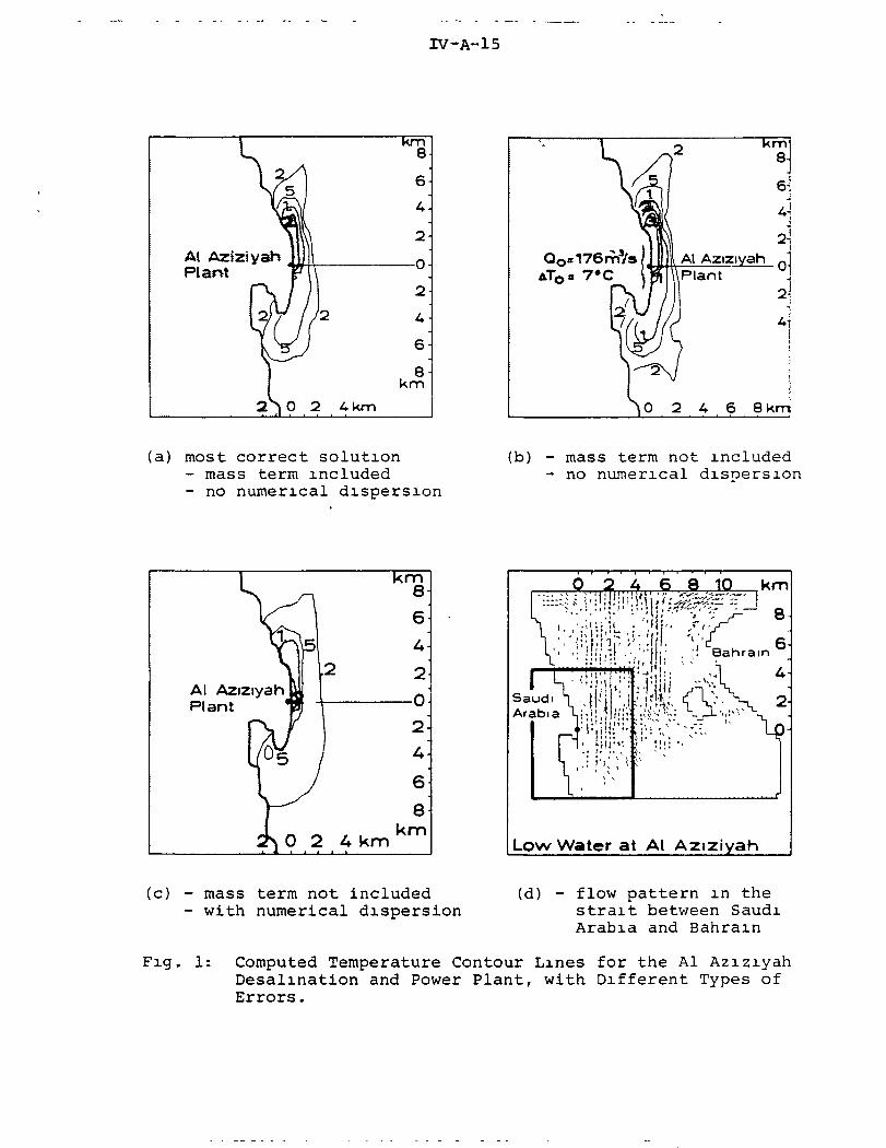
The effect on the temperature distribution around the source isdramatic; the temperature will in fact rise with each followingstep in time in the computations. The effect is shown inFigs. l,a, b and c, where results are presented obtained inconnection with a site selection study made for a combined de-salination and power plant on the east coast of Saudi Arabia.The discharge of this plant will be 176 m3/s with an excesstemperature of 7°C. Fig. l.a shows the most correct solution ;in which the mass term is included in the equation and whereno numerical dispersion is present. Fig. l.b shows the samesituation, now neglecting the mass term, but still withoutnumerical dispersion: high temperature around the outlet causesthe 1°C contour to stretch over a much larger area. Fig. l.cshows the same situation now neglecting the mass term and withnumerical dispersion. One observes that both errors almostcancel each other: the results resemble those of Fig. l.a. Soeven with two considerable errors the results may still lookreasonable! In Fig. l.d results from a hydrodynamic model areshown for the strait between Saudi Arabia and the island ofBahrain. The velocity field for the TD-model is taken fromthis HD-model.

Coupling Plume and TD-model

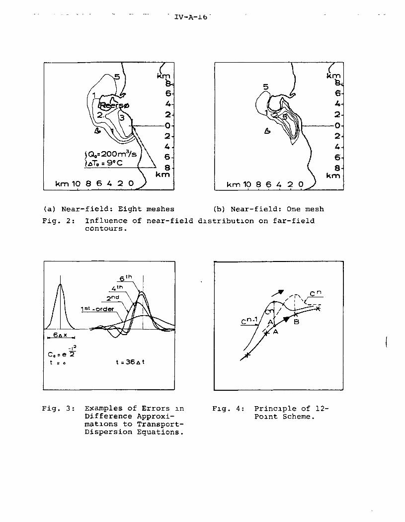
The mass error and, as we shall see, also numerical dispersioncan be avoided. Transferring the temperature distribution fromthe plume model to the TD-model presents a more principleproblem. The usual approach is to assume that waste heat is dis-tributed over a few grid spaces and uniformly mixed from bottomto surface. The integral value of excess temperature timesvolume, taken per unit time, is set equal to the waste heatdischarged, but different volume, excess temperature productsmay be taken to correspond to the same amount of waste heat.It is difficult to make this distribution equivalent to thatobtained in the plume model where the distribution is principlythree-dimensional. Using a different number of grid spacesfor the near field distribution gives different far-field con-tour lines. The difference is greatest close to the sourceand becomes less further away. However, with a very differentnear-field distribution the picture of the contour lines willbe very different. An extreme example is given in Figs. 2.aand b. The results shown are obtained in connection with thesite investigation for a 4000 MW nuclear plant in Denmark.Fig. 2.a shows the contour picture obtained with a near-fielddistribution over eight grid spacings, whereas in Fig. 2.bthe distribution is over only one grid spacing. Of course the

-5- GSR

IV-A-8

very high excess temperature in the last case will lead to a highrate of heat loss to the atmosphere and the contours cover asmaller area. Again numerical dispersion could mask the errorcaused by an incorrect near-field distribution.

The choice of near-field distribution in the TD-model must ofcourse be guided by the results obtained in the plume model,but because of the different character of the two models thetransfer will always be imperfect.

The problem outlined above is, however, not the only principleproblem in coupling a plume model to a TD-model. The plumemodel assumes a certain temperature of the ambient water.Characteristics of the plume such as entrainement and buoyancyare dependent on this ambient temperature. One should realisein this connection that the 'far-field1 is also present nearthe outlet. This is especially the case for a coastal outletwith an oscillating tidal current along the coast. In the caseof a power plant with a large waste heat discharge the tempera-ture in the area around the outlet will build up and theentraining water will already be heated. This leads us to acircular problem in modeling: in order to compute the near-fieldtemperature distribution by means of a plume model the ambienttemperature must be known, but in order to compute the ambienttemperature one must compute the far-field distribution and thisis in turn dependent on the near field distribution given by theplume. One is forced to spine sort of iterative procedure ifaccurate answers are to be obtained.

After having looked at these problems of coupling we can con-clude that our difficulties stem principally from handling theproblem in separate models and from differences in resolutionof these models. This approach is imposed by engineeringnecessity. The problem of difference in resolution may bereduced by using a model with varying resolution: detailed aroundthe outlet, with a coarser grid away from the outlet. A FiniteElement Model allows a net with small elements around the outletgradually changing to larger elements further away. In a FiniteDifference Model a change-of-scale can be used, using a localpatch of high resolution in an otherwise coarse grid.

The circular problem of the value of the ambient temperature tobe used in the plume computation is hard to overcome. One isin fact looking for a "complete" model, where the near-fieldand far-field temperatures are computed simultaneously. Attemptshave been made to develop such a model using the Marker-in-Celltechnique. The entire flow region in three dimensions isdivided into a sufficient number of cells and the computationprocedure is based on the approximate satisfaction of the inte-gral form of the conservation equations for each cell at every

GSR -6-

IV-A-9

time step; the approach is conceptually that of "box" modeling.The demand on computer storage and time is, however, excessiveand for engineering applications not acceptable.

Coupling with Ecological Models

Temperature is an important forcing function in biological andchemical processes. Ecological models can be applied to computethe consequences of discharges of waste heat. However, suchmodels usually deal with slowly varying processes with a timescale expressed in weeks and months. The information requiredhas for example a form as "number of days per year for which acertain temperature level is exceeded". There is a clear con-flict of time scales between the models for temperature distri-bution and the ecological models. The approach usually is tosimulate in the temperature distribution models a short periodthat is statistically equivalent to the period required in theecological model. This last period can be, for example, a year.This introduces a statistical interface between the temperaturedistribution models and the ecological model. Errors will beintroduced, if the quality or quantity of the data on which thestatistics are to be based, is insufficient.

There is also a conflict in the spatial scales between the HD-and TD-models and an ecological model. In a complex ecologicalmodel a large number of ordinary differential equations have tobe solved for each mesh considered. If a grid of the same meshsize as used in the HD- and TD-models would be used in order toobtain detailed information on fluxes, the cost of computationwould become prohibitive. An averaging of hydraulic conditionsmust be introduced with, as a consequence, a loss of accuracy.

For a more detailed discussion of the use of ecological modelsin power plant site studies we refer to the paper by K.I. DahlMadsen - Ref.[2]- in this Conference.

NUMERICAL TECHNIQUES AND ERRORS

In this section we shall limit the discussion to errors in theTD-models and techniques to avoid these. Not that the othermodels have no errors, but particularly in the TD-model theerrors are difficult to detect and the results may give a falseimpression of correctness. Moreover, the TD-model has a centralr61e in waste heat studies.

When the continuous differential equation of transport and dis-persion is represented on a discrete grid errors can be intro-duced. Well-known is the numerical dispersion that may be intro-duced. But although well-known it is difficult to avoid withoutintroducing other errors. We may in short recall how this error

-7- GSR

IV-A-10

is introduced. A simple finite difference approximation of theterms

1 Ix (3-1)-In

n+1 n n nto (c. - c )/At + u(c - c.^J/Ax (3.2)

introduces the truncation error

u(Ax - uAt) £-£ (3.3)

, which has the form of a dispersion term. The term depends onthe choice of the grid and the magnitude of the advective vel-ocity. Its value may be many times that of the physical dis-persion and may completely invalidate the results.

In order to avoid this error one may resort to higher orderdifference approximations. However, then a residual numericalradiation and skewness appear. The various effects are illus-trated in Fig. 3.

Numerical oscillations also may be introduced by use of an inap-propriate scheme. For example, the transport equation

1°- + u^ = 0 (3.4)at 3x • v '

may be approximated by the centred, second order differencescheme

n+1 n n+1 n v , n+1 n+1 n nfc - c

i f T 1

, .[c - c . , c - c , \

H (_! _ 2zi + _3 _ izl]2 \ Ax Ax /\ At At

= 0 (3.5)0

However, when initially c =0 for all 3 and u is constant, thisprovides ^

/I - u^\ ,(3.6)

= (-IP ^ c: (3.7)

GSR -8-

IV-A-11

which oscillates for all Courant numbers Cr = uAt/Ax, satisfying|Cr|<l.

Higher order approximations have the disadvantage that theyextend over more and more grid points with increasing orders ofapproximation. This presents problems at the boundaries. Arti-ficial assumptions for the approximation have to be made anderrors are introduced.

One method to avoid all such types of errors is to apply aLagrangian type of model. The advective term is then in factcut out by moving in a local frame with the local velocity ateach grid point. When this procedure is followed in a flowfield varying in time and space, the grid will distort tounwieldy forms. Therefore the local frame is moved only for onetime step and the information obtained is then transferred backto points in a fixed grid. One may also express it in a com-plimentary form: given a fixed grid at time to + At where wasthe information now in grid point B at time to. The principleis illustrated in Fig. 4. Following this principle a practicalmodel has been developed at the author's Institute.

The method requires a sophisticated interpolation technique todetermine the values of concentration (or temperature) in thepoints at time to, relative to the given fixed grid. The inter-polation used is based on a 12-point Everett interpolation.The "correctness" of this approach is best illustrated in a so-called rotation test in which a Gaussian distribution is rotatedin a two-dimensional grid around a center point located outsidethe distribution. Results are presented in Fig. 5. It may beobserved that the shape is fairly well preserved in this rathertough test.

This type of approach may also be used with a Finite ElementModel. As the F.E.M. technique does not give solutions in dis-crete grid points, but as solution surfaces over elements, theinterpolation is not required (- or is in fact already includedin the F.E. M. technique). Clearly higher order elements arenecessary to obtain results without erroneous dispersion. How-ever, compared with finite difference schemes F.E.M. models areusually found to be considerably more expensive for time varyingsolutions.

The 12-point scheme introduced above also requires special for-mulations at the boundaries, but satisfactory approximations canbe obtained. Simply using the correct zero concentration valuefor points beyond a land boundary gives good results. This isdemonstrated in a so-called L-test in Fig. 6.a.

The propagation of a circular distribution around a sharp corneris depicted for a sequence of time steps. One observes that the

-9- GSR

IV-A-12

circular form is preserved for the stretch before the corner.It is distorted beyond the corner, but this is physically re-alistic. The deformation is caused by the flow field aroundthe corner. In order to illustrate how an incorrect schemewith considerable numerical dispersion may distort a circulardistribution, corresponding results of such a scheme are shownin Fig. 6.b.

At open water boundaries also special attention is required.However, satisfactory results are usually obtained when suchboundaries are recognized as being either inflow or outflowboundaries, with an assumption on the mixing conditions in thewater body beyond the boundary.

A quite different method, that probably is the most accurate,is based on a spectral technique. The method is developed foran application in atmospheric pollution by Christensen andPram - Ref. 4. The technique was applied to hydraulic problemsin the author's institute. The method is very accurate, butcomputer costs are about four t'imes as high as for the 12-pointscheme. The method also has limitations with regard to resol-ution of realistic topographies. In short the technique is asfollows: It is assumed that c can be approximated by a finiteFourier representation

f(x,t) = I A(k,t) elkx, with i = /^T (3.8)k

For a given continuous function f(x,t) one can always findA(k,t) such that f(x,t) = c(x,t) on grid points x = jAx:

j J

A(k,t) = ̂ I C;](t) e~ik jAx (3.9)

The simple equation

|f + uff = 0 .10,

transforms to

3Afo'fc) + u ik A (k,t) = 0 (3.11)cCC

From this equation A(k,t) can be computed at each new time nAtwith A(k,t) given, c can be obtained from an inverse Fourier-transform. The point here is to note that the advection termin (3.11) is not approximated by a finite difference form sothat numerical dispersion is avoided.

GSR -10-

IV-A-13

DISCUSSION

A discussion of modeling problems and errors may leave the readerwith a rather gloomy impression of the whole modeling effort.And there is more, in addition to the problems discussed thereare the difficulties encountered when dispersion coefficient andheat transfer coefficients have to be selected. Field investi-gations before the plant has been constructed can only give avery limited impression of the mixing characteristics of thereceiving water body, as discharge volume, discharge momentumand buoyancy cannot be represented.

However, if the models are used with an awareness of the inac-curacies and if sensitivity tests are made for the importantparameters, usefull predictions can be made. Such predictionswould allow design considerations of outlet-intake constructioncost against possible recirculation as discussed in the paperby Schr0der - Ref. [5] - in this Conference, and an evaluation ofecological consequences.

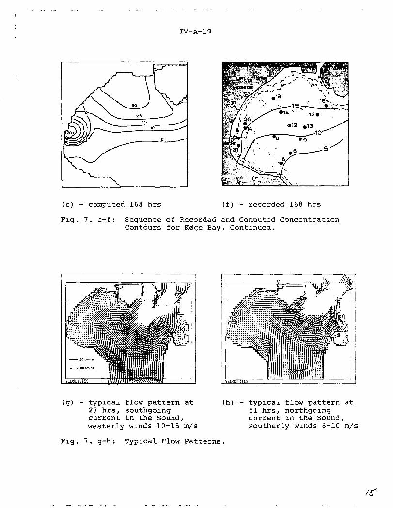
We may underline the above statement with a final result. Thepossibility of simulating the transport-dispersion process overan extended period of time in a realistic topography is illus-trated in Fig. 7. The transport and dispersion of a conservativesubstance with an irregular release - 16 hrs out of 24 per day -is simulated. The area concerned is K0ge Bay, south of Copen-hagen. In a sequence of plots the development of the concen-tration field from an initial distribution to the situationafter one week is shown. The results after one week are com-pared to measurements. One may observe that after having beenthrough considerable changes, the characteristics of the fieldafter seven days compare well with measurements.

ACKNOWLEDGEMENT

The present paper is based on research by the staff of the Com-putational Hydraulics Centre of the Danish Hydraulic Institute.

REFERENCES

1. Abraham, G. 'Methodologies for Temperature Impact Assessment1.European Course on Heat Disposal from Power Generation inthe Water Environment. Delft Hydraulics Laboratory, Delft,the Netherlands, 1975.

2. Dahl Madsen, K.I., "Modeling the Influence of ThermalEffluents on Ecosystem Behaviour". This Conference.

-11- GSR

IV-A-14

Abbott, M.B., "Computational Hydraulics: A Short Pathology".Journal of Hydraulic Research 14 (1976) No. 4.

Christensen, 0. and Prahm, L.P., "A Pseudospectral Model forDispersion of Atmospheric Pollutants". Danish MeteorologicalInstitute, Lyngbyvej 100, Copenhagen, Denmark. 1976.

Schr0der, H., "Selection of Alternative Coastal Locations".This Conference.

GSR -12-

IV-A-15

Al AztztyahPlant

xm8

6

A

2-Al Aziziyah

APlant•0

2

A

0 2 A 6 8km

(a) most correct solution- mass term included- no numerical dispersion

(b) - mass term not included- no numerical disnersion

Al AziziyahPlant Saudi S

Arabia X;

fir6 8 1Q km

; f li.r& ̂

Low Water at At Aziziyah

(c) - mass term not included- with numerical dispersion

(d) - flow pattern in thestrait between SaudiArabia and Bahrain

Fig, 1: Computed Temperature Contour Lines for the Al AziziyahDesalination and Power Plant, with Different Types ofErrors.

IV-A-16

km 10 8 6 A 2 0km

km 10 8 6 A 2 0

(a) Near-field: Eight meshes

Fig. 2:

(b) Near-field: One mesh

Influence of near-field distribution on far-fieldcontours.

,2

2~t = t =36A

Fig. 3: Examples of Errors inDifference Approxi-mations to Transport-Dispersion Equations.

Fig. 4: Principle of 12-Point Scheme.

IV-A-17

1004 t

150At

200At

DIRECTION OFROTATION

50 At

CORRECTSOLUTION

NUMERICALSOLUTION

Fig. 5: Rotation Test,12-Point Scheme.

120At 180At

96 At

60At

150 At 200 At

80At

60 At

2Atc Lfn«s of C = 1

(a) 12-Point Scheme (b) Scheme with Numericaldispersion

Fig. 6: L-Test of Different Difference Schemes.

IV-A-18

(a) - recorded 0 hrs (b) - computed 23 hrs

(c) - computed 71 hrs (d) - computed 111 hrs

Fig. 7. a-d: Sequence of Recorded and Computed ConcentrationContours for K0ge Bay.Source: 16 hrs on, 8 hrs off per 24 hrs, with2 x 24 hrs off during weekend between 88 hrsand 144 hrs.Load: 168 gram/sec.

IV-A-19

(e) - computed 168 hrs (f) - recorded 168 hrs

Fig. 7. e-f: Sequence of Recorded and Computed ConcentrationContours for K0ge Bay, Continued.

£-•- "'MmtS&S&Ssfa

VELdCiTlES

(g) - typical flow pattern at27 hrs, southgoingcurrent in the Sound,westerly winds 10-15 m/s

(h) - typical flow pattern at51 hrs, northgoingcurrent in the Sound,southerly winds 8-10 m/s

Fig. 7. g-h: Typical Flow Patterns.