Numerical modelling of two dimensional heat transfer in … · 2011-03-08 · are developed basic...

Abstract— Solving the differential equation of heat conduction

the temperature in each point of the body can be determined. Howe-ver, in the case of bodies with boundary surface of sophisticated geometry no analytical method can be used. In this case the use of numerical methods becomes necessary. The finite element method is based on the integral equation of the heat conduction. This is obtai-ned from the differential equation using variational calculus. The temperature values will be calculated on the finite elements. Then, based on these partial solutions, the solution for the entire volume will be determined. Using this method we can divide into elements also fields with any border. Also, numerical modelling with boun-dary elements is used for analysis of heat conduction. In this paper are developed basic ideas of numerical analysis with finite elements and boundary (constant) elements of conductive thermal fields gene-rated or induced into solid body in steady state regime. The tempera-ture distribution in some solid bodies and in pipe insulation is analyzed using analytical method and finite element and boundary element methods, implemented in two computer programs develo-ped by the author. This shows the good performance of the proposed numerical models.

Keywords— Heat transfer, Steady state regime, Finite elements,

Boundary elements, Variational calculus, Numerical models, Com-puter programs.

I. INTRODUCTION

ODERN computational techniques facilitate solving pro-blems with imposed boundary conditions using diffe-

rent numerical methods [6], [7], [9], [16–19]. Numerical ana-lysis of heat transfer [12], [13] has been independently though not exclusively, developed in three main streams: the finite differences method [22], [24], the finite element method [1], [20], [23] and the boundary element method [3], [4], [5].

The finite differences method (FDM) is based on the diffe-rential equation of the heat conduction, which is transformed into a numerical one. The temperature values will be calcu-lated in the nodes of the network. Using this method conver-gence and stability problem can appear.

The finite element method (FEM) and the boundary ele-ment method (BEM) is based on the integral equation of the heat conduction. This is obtained from the differential equa-tion using variational calculus. In first case the temperature

Ioan Sarbu is currently a Professor and Department Head at the Building

Services Department, “Politehnica” University of Timisoara, 300233 ROMANIA, e-mail address: [email protected]

values will be calculated on the finite elements. Then, based on these partial solutions, the solution for the entire volume will be determinated. Using this method we can divide into elements also fields with unregulated border. In the BEM case only the boundary is discretized into elements and internal point position can be freely defined.

In this paper the temperature distribution is analyzed in the solid bodies, with linear variation of the properties, using the FEM and the BEM.

II. ANALYTICAL MODEL OF HEAT CONDUCTION

The temperature in a solid body is a function of the time and space coordinates. The points corresponding to the same tem-perature value belong to an isothermal surface. This surface in a two dimensional Cartesian system is transformed into an isothermal curve.

The heat flow rate Q represents the heat quantity through an isothermal surface S in the time unit:

sqQS∫= d (1)

where the density of heat flow rate q is given by the Fourier law:

tn

tq grad λλ −=−=

∂∂

(2)

in which λ is the thermal conductivity of the material. The thermal conductivity of the building materials is the

function of the temperature and variation can accordingly be expressed as:

( )[ ]00 +1λλ ttb −= (3)

in which: λ0 is the thermal conductivity corresponding to the t0 temperature; b – material constant.

If there is heat conduction within an inhomogeneous and anisotropy material, considering the heat conductivity con-stant in time, the temperature variation in space and time is given by the Fourier equation:

0λλλτ

ρ Qz

t

zy

t

yx

t

x

tc zyx +

+

+

=

∂∂

∂∂

∂∂

∂∂

∂∂

∂∂

∂∂ (4)

in which: t is the temperature; τ – time; ρ – material density; c – specific heat of the material; λx, λy, λz – thermal conduc-tivity in the directions x, y and z; Q0 – power of the internal sources.

To solve the differential equations it is necessary to have supplementary equations. These equations contain the geome-

Numerical modelling of two dimensional heat transfer in steady state regime

Ioan Sarbu

M

Issue 3, Volume 5, 2011 435

INTERNATIONAL JOURNAL of ENERGY and ENVIRONMENT

trical conditions of the analysis field, the starting conditions (at τ = 0) and the boundary conditions. The boundary conditions (Fig. 1) describe the interaction between the analyzed field and the surroundings. In function of these interactions different conditions are possible:

Fig. 1 Boundary conditions

– the Dirichlet (type I) boundary conditions give us the tem-perature values on the boundary surface St of the analyzed field like a space function constant or variable in time:

( ) τ, , , zyxft = (5)

– the Neumann (type II) boundary conditions gives us the value of the density of heat flow rate through the Sq boundary surface of the analyzed field:

zzyyxx nz

tn

y

tn

x

tq

∂∂

∂∂

∂∂

λλλ ++= (6)

in which: nx, ny, nz are the cosine directors corresponding to the normal direction on the Sq boundary surface. – the Cauchy (type III) boundary conditions gives us the ex-ternal temperature value and the convective heat transfer coefficient value between the Sα boundary surface of the body and the surrounding fluid:

( ) zzyyxxe nz

tn

y

tn

x

ttt

∂∂

∂∂

∂∂

λλλ α ++=− (7)

in which: α is yhe convective heat transfer coefficient from Sα to the fluid (or inversely); te –fluid temperature.

The analytical model described by the equations (4)…(7) can be completed with the material equations which provide us information about variation of the material properties de-pending on temperature. In the case of matertials with linear physical properties, this equations (λ = const.) are not used in the model.

Solving the differential equation of the heat conduction (4) we can determine the temperature values in each point of the body. However, in the case of bodies with boundary surface of sophisticated geometry, the equation (4) cannot be solved using analytical methods. In this case numerical methods should be applied. The increasing availability of computers has also lead into the direction of more frequent use of these methods.

III. FORMULATION OF NUMERICAL MODEL WITH FINITE

ELEMENTS

To use the FEM, the transformation of the equations (4)… (7) into integral model is necessary. To realize this transfor-mation we can use variation calculus.

The temperature t(x, y, z, τ ) which represent a solution for the differential heat conduction equation (4) and for condi-tions (5), (6), (7), also represents a solution for the steady state equation of the V field:

0δ =F (8)

which is equivalent, from mathematical point of view, with the equations (4)…(7) and were F is the functional of the heat conduction.

+d 2

1222

Vz

t

y

t

x

tF zyx

V

+

+

= ∫ ∂

∂λ∂∂λ

∂∂λ

StttStqVtQt

cqS S

e

V

d2

1 d d ρ + 0 ∫ ∫∫

−+−

−

α

ατ∂

∂ (9)

in which: Q0 is positive when the internal sources produce heat and negative when these sources absorb heat; q is posi-tive when the body receives heat and negative when the body yields heat to the surrounding fluid; α is positive on the surfaces where the heat transfer happens from the body to the fluid and it is negative inversely.

The minimization of the functional is done correspondingly to each finite element. The solution for the entire field is obtai-ned joining the partial solutions.

Though the heat conduction is carried out within three–dimensional bodies, the temperature distribution variation is significant only in certain directions. Thus, the analysis of temperature distribution in bars, plain or cylindrical walls is done using a two–dimensional model.

In the steady state heat transfer processes the temperature does not depend on the time, thus in the equation (9)

0/ =∂∂ τt . In addition, at two–dimensional problems, the tem-perature does not vary on z direction, thus 0/ =∂∂ zt .

A. General Equations of the FEM

In our case the equation (9) can be expressed as:

∫ −

−

+

+

=

V

zyx VtQz

t

y

t

x

tF d

2

10

222

∂∂λ

∂∂λ

∂∂λ

StttSqtS

e d2

1d

qS∫∫

−+−α

α (10)

Taking into account that the temperature function is not continuous on the entire field, the equation (10) can be inte-grated only on the finite elements. On the entire field the functional F can be written as a sum of m functionals Fe, where m is the number of finite elements:

∑=

=m

e

eFF1

(11)



∑ ∫∫=

−−

∂∂+

∂∂=

m

10

22

dd2

1

e V

e

V

e

y

e

x

ee

VtQVy

t

x

tF λλ

−+− ∫ ∫qe eS S

eeee StttSqt

α

α d2

1d (12)

where the “e”exponent refers to a finite element. For a given finite element the temperature te can be calcu-

lated based on the temperature values in the nodes:

[ ] enne tNtNtNtNt =+++= ...2211 (13)

where: n is the number of the finite element nodes; [N] – form matrix of the finite element; te – vector of the temperature values in the nodes.

In the expression (12) appear the partial derivates of the temperature, therefore the equation (13) should be derived:

[ ] e

n

n

n

e

e

tJ

t

t

t

y

N

y

N

y

Nx

N

x

N

x

N

y

tx

t

B =

=

= 2

1

21

21

...

...

∂∂

∂∂

∂∂

∂∂

∂∂

∂∂

∂∂∂∂

(14)

If the thermal conductivities are written in matrix form:

[ ]

=

y

xD

λλ0

0 (15)

then equation (12) can accordingly be expressed as:

[ ] ( ) [ ][ ] [ ] [ ] ∫∫∫ +−−=qeee S

e

V

eoeT

e

V

e StNqVtNQVtJDtJF ddd2

1

[ ] ( ) [ ] ∫ ∫−+e eS S

eee StNtStN

α α

ααdd

22 (16)

Because

[ ] ( ) [ ][ ] ( ) [ ] ( ) [ ] ( ) [ ] [ ] e

TTee

Tee

TTe

Te

tNNttNtNtN

JttJ

==

=2

(17)

the equation (16) can be expressed as:

[ ] [ ][ ] [ ] [ ] ∫∫∫ +−−=qeee S

e

V

eoeTT

e

V

e StNqVtNQVtJDJtF ddd2

1

[ ] [ ] [ ] ∫ ∫−+e eS S

eeeTT

e StNtStNNt

α α

ααdd

2 (18)

If we derive the matrix equation (18) the further equation is obtained:

[ ] [ ][ ] [ ] [ ] −

+= ∫∫ e

S

TT

Ve

e

tSNNVJDJt

F

ee α

α∂∂

dd

[ ] [ ] [ ]∫∫∫ −−−eqe S

Te

S

T

Ve

To SNtSNqVNQ

α

α ddd (19)

Because dAhdV = and dLhdS = , where h is the thick-

ness of the finite element, dA – aria of the finite element and dL – length of the finite element side, result:

[ ] [ ][ ] [ ] [ ] −

+= ∫∫ e

L

TT

Ae

e

tLNNAJDJht

F

ee

dd α∂∂

[ ] [ ] [ ]∫∫∫ −−−eee L

Te

L

T

A

To LNthLNqhANQh ddd α (20)

The finite element thickness h is considered constant and equal with 1 m. The equation (20), can be written as in com-pressed form:

[ ] ptkt

Fe

e

e

−=∂∂

(21)

where:

[ ] [ ] [ ][ ] [ ] [ ]∫∫ +=ee L

T

A

T LNNhAJDJhk

α

α dd (22)

[ ] [ ] [ ]∫∫∫ ++=eqee L

Te

L

T

A

T LNthLNqhANQhp

α

α ddd0 (23)

in which: [k] is the matrix of the heat conduction correspon-ding to a finite element, the first term is related to conduction and the second term to convection on the Lαe side of the Sαe boundary surface; p – vector of heat sources containing the internal sources Q0, the density of heat flow rate q on the Sqe boundary surface and convection on the Sα boundary surface.

The minimization of the F functional supposes the equality with zero of the first derivate in each point of the studied field. Taking into account of (11) results:

∑∑==

==m

e e

m

e

e

t

FF

tt

F

11 ∂∂

∂∂

∂∂

(24)

Introducing equation (21) in (24) we obtain the equation system corresponding to the entire field: [ ] PtK = (25)

where:

[ ] [ ] ∑∑ ==m

1

m

1

;k pPK (26)

in which: [K] is matrix of heat conduction of the entire field; P – vector of heat sources corresponding to studies field; t − vector of unknown temperatures. The equation (25) represents the form with finite element of the differential equation of heat conduction, which contains a number of equations equal to the number of the nodes with unknown temperature values.

B. Matrix of the Heat Conduction

If we use finite elements with triangle form in a certain point of the finite element, using the relation (13) the te temperature (Fig. 2), can be written as:

[ ] [ ] e

k

j

i

kjikkjjiie tN

t

t

t

NNNtNtNtNt =

=++= (27)

in which: ti, tj, tk are the temperatures in i, j, k nodes (nodes of triangle finite element); [N] – form matrix of the finite ele-ment [17], [19].



Fig. 2. Finite element with triangle form

The conduction matrix of a finite element is:

[ ] [ ] [ ]21 kkk += (28)

where:

[ ] [ ] [ ][ ] [ ] [ ] [ ]∫∫ ==ee L

T

A

T LNNhkAJDJhkα

α d;d 21 (29)

The [J] matrix, using the relation (14) can be expressed as:

[ ] e

k

j

i

kji

kji

e

e

tJ

t

t

t

y

N

y

N

y

Nx

N

x

N

x

N

y

tx

t

B =

=

=

∂∂

∂∂

∂∂

∂∂

∂∂

∂∂

∂∂∂∂

(30)

If we derive the elements of the form matrix:

[ ]

==

kji

kji

ekji

kji

ccc

bbb

A

y

N

y

N

y

Nx

N

x

N

x

N

J2

1

∂∂

∂∂

∂∂

∂∂

∂∂

∂∂

(31)

where Ae is the area of the finite element, and the b respective c can be written as [19]:

ijkkijjki

jikikjkii

xxcxxcxxc

yybyybyyb

−=−=−=−=−=−=

;;

;; (32)

Consequently, the [J] matrix is constant. Because the λx and λy thermal conductivities do not vary for a finite element, the [D] matrix is also constant, thus:

[ ] [ ] [ ][ ] [ ] [ ][ ]∫ ==eA

eTT AJDJhAJDJhk d1 (33)

Introducing the expression of [J] matrix from (31) and the expression of [D] matrix from (15) in (33) results:

[ ]

+++++++++

=

kkykkxjkyjkxikyikx

kjykjxjjyjjxijyijx

kiykixjiyjixiiyiix

e ccbbccbbccbb

ccbbccbbccbb

ccbbccbbccbb

A

hk

λλλλλλλλλλλλλλλλλλ

41(34)

The matrix [k2] from the equation (28) can be written as:

[ ] L

NNNNNN

NNNNNN

NNNNNN

hkeL

kkjkik

kjjjij

kijiii

d2 ∫

=α

α (35)

Using the L – natural coordinates and considering that convective heat transfer exists on the jk side of the finite ele-ment, we obtain:

[ ] L

LLLL

LLLLhkeL

kkkj

kjj d

0

0

000

j2 ∫

=α

α (36)

To solve the equation (36), the following relation should be used:

( )!1

)( ! !d

++−

=∫ βαβαβα ij

X

X

ji

XXxLL

j

i

(37)

Consequently for products with the same indices j or k is obtained:

( ) 3!1+0+20! 2!

ddd 2 ee

L

j

L

kk

L

jjL

LLLLLLLLL

eee

αα

ααα

==== ∫∫∫ (38)

and for products with different indices j and k is obtained:

( ) 6!1+1+1

1! 1!dd e

e

L

jk

L

kj

LLLLLLLL

ee

αα

αα

=== ∫∫ (39)

Substituting into equation (36) results:

[ ]

=210

120

000

62eLh

k αα (40)

If convective heat transfer exists the ij or ki sides of the finite element are:

[ ] [ ]

=

=201

000

102

6;

000

021

012

6 22ee Lh

kLh

k αα αα (41)

The matrix [k2] exists only in the case when at least, o none side of the finite element heat transfer is realized by con-vection.

C. Vector of the Heat Sources

This vector is based on the equation (23) from three terms, which can be calculated using the L–natural coordinates. Sup-posing that Q0 is constant for a finite element, using the follo-wing relation:

( ) e

A

kji AALLLe

2!2+++

! ! !d

γβαγβαγβα =∫ (42)

we obtain that:

[ ] =

== ∫∫ee A

k

j

i

o

A

ToQ A

N

N

N

hQANQhp dd

=

= ∫1

1

1

3d eo

Ak

j

i

o

AhQA

L

L

L

hQe

(43)

The second term, for a certain density of heat flow rate, corresponds to the heat transfer on the boundary surface of the



studied field. Supposing that the body receives the heat flow through Lki = Lqe side of the finite element, using the relation (37) we obtain:

[ ]

=

=

== ∫∫∫1

0

1

2d0d0d qe

Lk

i

Lk

i

L

Tq

hqLL

L

L

hqL

N

N

hqLNqhpqeqeqe

(44)

The third term, from the equation (23), corresponds to con-vective heat transfer on the jk (Ljk = Lαe) side of the finite element. Using the relation (37) we obtain:

[ ] =

== ∫∫ee L

k

je

L

Te L

N

NthLNthpαα

ααα d

0

d

=

= ∫1

1

0

2d

0ee

Lk

je

LthL

L

Lthe

αααα

(45)

It could be observed that the element zero in the vector (44) and (45) can occupy any position, corresponding to the side of finite element with heat transfer.

Based on the equation systems obtained for the finite ele-ments, they can realize the equation system for the entire stu-died field. This system can be solved using analytical or itera-tive methods.

In present there are different programms on the software market which permit numerical analysis of the temperature distribution (e.g. WAEBRU) but these programms are too expensive and our department cannot buy them. In this con-text to analyze the temperature distribution in a solid body under steady state heat transfer regime using the numerical model presented above the TAFEM software has been deve-loped by author of this article. The equation system is solved using the Gauss method.

IV. DEVELOPMENT OF NUMERICAL MODEL WITH BOUNDARY

ELEMENTS

In the case of a plain wall, inside the analysis field, the heat conductivity in steady state regime is modelled by the Laplace equation [4]:

02 =∇ t (46) On Γt portion of boundary Γ of the analysis field Dirichlet

boundary conditions are imposed and leftoner portion Γq Neumann boundary conditions are imposed.

In order to determine the temperature on the boundary of the analysis field one uses the following integral equation [3], [4], [6]:

∫∫Γ

∗∗

Γ

Γ∂

∂=Γ+ )(d),()(

)(d),()()()(oo

oooo

XXun

XtXXvXttc ζζζζ (47)

where: ζ is the point in which one writes the integral equation

(source point); c(ζ) − a coefficient; oX − the current integra-

tion point; ( )

=∗ ),(/1π2/1),(

ooXrXu ζζ − fundamental

solution; nuv ∂∂ /∗∗ = − normal derivative of this solution.

The distance r(ζ,oX ) between the current point

oX and the

source point ζ is calculated with the relation:

2

12o2oo

)()()()(),(

−+

−= ζζζ yXyxXxXr (48)

Boundary Γ is discretized into N constant boundary ele-ments for which one considers temperatures tj, respectively the normal derivative (∂t/∂n)j constant and equal to the mid point (node) value of the element. Thus the integral equation is obtained under the following discretized form:

∑ ∫ ∑ ∫= Γ = Γ

∗∗ Γ

∂∂=Γ+

N

j

N

j jjii

j j

XXun

tXXvttc

1 1

oooo

)(d),()(d),( ζζ (49)

or

∑ ∑= =

∂=+N

j

N

j jijjijii n

tBtAtc

1 1 dˆ (50)

in which coefficients $Aij and Bij have the expressions:

∫∫Γ

∗

Γ

∗ ≠Γ=Γ=jj

jiXXuBXXvA ijij )(d),();(d),(ˆoooo

ζζ (51)

When i = j these become:

−=+=2

n112

;ˆ2

1 iiiiiiii

llBAA

π (52)

Explicitely, equation (50) generates a liniar and compatible system of N equations with 2N unknowns [tj and (∂t/∂n)j] and after implementing the boundary conditions, the number of unknowns is reduced to N. In the case of constant boundary

elemnents, coefficient ci has the value 1/2. Coefficients $Aij and

Bij from (51) is computed using a Gauss quadrature [8], [19]:

∑∑=

∗

=

∗ ==m

kkk

jij

m

kkk

jij wu

lBwv

lA

11 2;

2ˆ (53)

in which lj is the length of the j boundary element. Introducing notations: nx = cos(n, x); ny = cos(n, y) and

using, for ∀oX ∈Γ, the parametric equations:

[ ]1,1 ,; −∈+=+= ξξξ DCyBAx (54)

where: x∈[xj, xj+1] and y∈[yj, yj+1], the following relations are obtained:

2222

;CA

An

CA

Cn yx

+=

+

−= (55)

in which (xj, yj) and (xj+1, yj+1) are the extremities of the boun-dary element j.

The analysis field is transformed into a dimensionless one by replacing the dimensional variables (x, y) with dimension-less ones (x∗, y∗):

maxmax

;x

yy

x

xx == ∗∗ (56)

in which xmax is the maximum extension of the analysis field after axis Ox.



In order to determine the temperature inside of the analysis field is used the integral representation:

∫ ∫Γ Γ

∗∗ Γ−Γ∂

∂= )(d),()()(d),()(

)(ooooo

*

o

XXvXtXXun

Xtt iii ζζζ (57)

in which: ,oΩ∈iζ where

oΩ represent the inside of the ana-

lysis field Ω ( Ω =oΩ UΓ).

After the discretization of boundary Γ into N constant boun-dary elements one obtains the integral equation under discre-tized form:

∑ ∫ ∑ ∫= Γ = Γ

∗∗ Γ−Γ

∂∂=

N

j

N

jiji

jii

j j

XXvtXXun

tt

1 1

oooo

*)(d),()(d),()( ζζζ (58)

which can be writhen as such:

∑∑==

−

∂∂=

N

jjij

j

N

jiji tA

n

tBt

11*

(59)

Coefficients ijij BA and are evaluated using a Gauss qua-

drature:

∑∑=

∗

=

∗ ==m

kkk

jijk

m

kk

jij wu

lBwv

lA

11 2;

2 (60)

in which: m is the number of Gauss type points; wk − weight coefficients.

Temperatures ti from points ζi are easily determined taking into account that values tj and (∂t/∂n*)j are known on the ana-

lysis field boundary, and coefficients ijij BA and are computed

with equation (54). By knowing values tj and ti of the temperature on the ana-

lysis field boundary, the group of coordinate points (x∗, y∗) for which t = const. represents the isothermal curves.

The numerical model based on BEM has been implemented in computer program TABEM, realized in Fortran program-ming language, for IBM–PC compatible systems.

V. APPLICATIONS

A. Temperature Distribution in Orthotropic Body

The temperature distribution is analyzed in a solid body 500×400 mm sectional dimensions (Fig. 3). The body receives heat flow on two sides: qx = 2320 W, qy = 928 W. On the other two sides the body transmit heat by convection αx = αy = 23.2 W/(m2⋅K). The material of the body has orthotropic properties with the following values of the thermal conductivies: λx = 11.6 W/(m⋅K), λy = 5.8 W/(m⋅K).

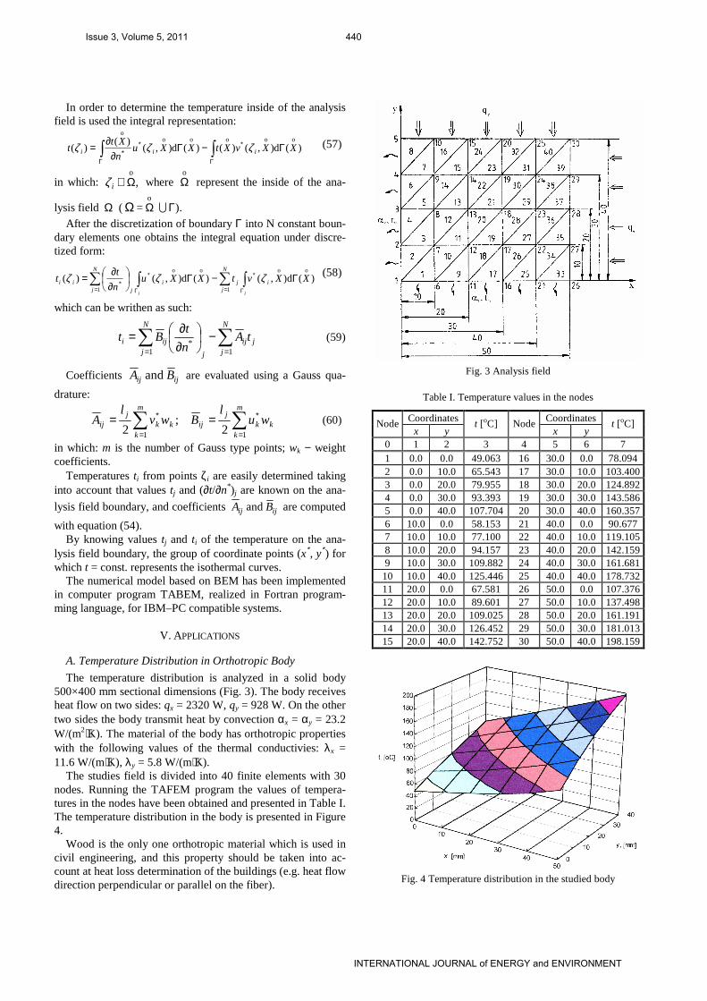
The studies field is divided into 40 finite elements with 30 nodes. Running the TAFEM program the values of tempera-tures in the nodes have been obtained and presented in Table I. The temperature distribution in the body is presented in Figure 4.

Wood is the only one orthotropic material which is used in civil engineering, and this property should be taken into ac-count at heat loss determination of the buildings (e.g. heat flow direction perpendicular or parallel on the fiber).

Fig. 3 Analysis field

Table I. Temperature values in the nodes

Coordinates Coordinates Node x y

t [oC] Node x y

t [oC]

0 1 2 3 4 5 6 7 1 0.0 0.0 49.063 16 30.0 0.0 78.094 2 0.0 10.0 65.543 17 30.0 10.0 103.400 3 0.0 20.0 79.955 18 30.0 20.0 124.892 4 0.0 30.0 93.393 19 30.0 30.0 143.586 5 0.0 40.0 107.704 20 30.0 40.0 160.357 6 10.0 0.0 58.153 21 40.0 0.0 90.677 7 10.0 10.0 77.100 22 40.0 10.0 119.105 8 10.0 20.0 94.157 23 40.0 20.0 142.159 9 10.0 30.0 109.882 24 40.0 30.0 161.681 10 10.0 40.0 125.446 25 40.0 40.0 178.732 11 20.0 0.0 67.581 26 50.0 0.0 107.376 12 20.0 10.0 89.601 27 50.0 10.0 137.498 13 20.0 20.0 109.025 28 50.0 20.0 161.191 14 20.0 30.0 126.452 29 50.0 30.0 181.013 15 20.0 40.0 142.752 30 50.0 40.0 198.159

Fig. 4 Temperature distribution in the studied body



B. Temperature Distribution in Pipe Insulation

The temperature distribution in pipe insulation was ana-lyzed (Fig. 5) using the TAFEM program. The calculus was made for a pipe with 800 mm nominal diameter and the hot water temperature was 150 °C. The ambient temperature was considered 1°C.

Fig. 5 Structure of insulation

1–pipe wall; 2a, 2b – insulation layers; 3–protection coat

To obtain results which describe the real situation as exactly as possible the convective heat transfer coefficient on the external insulation surface was considered variable with values between 10 and 25.6 W/(m2⋅K).

In Figures 6 and 7 the analyzed field and the temperature distribution are presented in the pipe section. It can be obser-ved that duet to the variable boundary conditions on the insu-lation surface the isotherm curves are not circular curves which are obtained when the classical calculus is used.

Fig. 6. Analysis field

Fig. 7. Temperature distribution in pipe insulation

C. Temperature Distribution in Metallic Plaque

In figures 8 and 9 are considered two variants of a metallic plaque, with dimensions 40×40×70 mm, for which one deter-mines the temperature field using BEM and analytical method (ANM). In figures 10 and 11 are presented the dimensionless

analysis domains together with mixed boundary conditions for these boundaries.

Fig. 8 Metallic plaque

Fig. 9 Metallic plaque with a semicylindrical cut–out

Fig. 10 Boundary conditions for metallic plaque

Fig. 11 Boundary conditions for metallic plaque

with semicylindrical cut–out



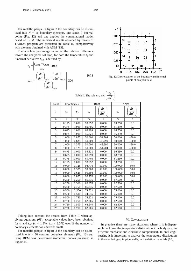
For metallic plaque in figure 2 the boundary can be discre-tized into N = 16 boundary elements, one states 9 internal points (Fig. 12) and one applies the computational model based on BEM. The numerical results obtained by means of TABEM program are presented in Table II, comparatively with the ones obtained with ANM [13].

The absolute percentage value of the relative difference toward the analytical solution, for both the temperature εt and it normal derivative εndt is defined by:

100ε

;100ε

*

**

⋅

∂∂

∂∂−

∂∂

=

⋅−

=

ANM

BEMANMndt

ANM

BEMANMt

n

tn

t

n

t

t

tt

(61)

Fig. 12 Discretization of the boundary and internal points of analysis field

Table II. The values tj and

jn

t

∂∂

*

Point Coordinates BEM ANM

j ∗jx ∗

jy tj j

n

t

∂∂

* tj

jn

t

∂∂

*

0 1 2 3 4 5 6 1 0.125 1.000 93.052 0.000 93.750 0.0 2 0.375 1.000 80.705 0.000 81.250 0.0 3 0.625 1.000 68.299 0.000 68.750 0.0 4 0.875 1.000 55.821 0.000 56.250 0.0 5 1.000 0.875 50.000 –51.704 50.000 –50.0 6 1.000 0.625 50.000 –48.290 50.000 –50.0 7 1.000 0.375 50.000 –48.290 50.000 –50.0 8 1.000 0.125 50.000 –51.704 50.000 –50.0 9 0.875 0.000 55.821 0.000 56.250 0.0 10 0.625 0.000 68.299 0.000 68.750 0.0 11 0.375 0.000 80.705 0.000 81.250 0.0 12 0.125 0.000 93.052 0.000 93.750 0.0 13 0.000 0.125 98.776 50.000 100.000 50.0 14 0.000 0.375 99.308 50.000 100.000 50.0 15 0.000 0.625 99.308 50.000 100.000 50.0 16 0.000 0.875 98.776 50.000 100.000 50.0 17 0.250 0.250 86.836 0.000 87.500 0.0 18 0.250 0.500 86.876 0.000 87.500 0.0 19 0.250 0.750 86.836 0.000 87.500 0.0 20 0.500 0.,250 74.521 0.000 75.000 0.0 21 0.500 0.500 74.536 0.000 75.000 0.0 22 0.500 0.750 74.521 0.000 75.000 0.0 23 0.750 0.250 62.205 0.000 62.500 0.0 24 0.750 0.500 62.240 0.000 62.500 0.0 25 0.750 0.750 62.205 0.000 62.500 0.0

Taking into account the results from Table II when ap-

plying equations (61), acceptable values have been obtained for εt and εndt (εt < 1.3%, εndt < 3.5%) even if the number of boundary elements considered is small.

For metallic plaque in figure 3 the boundary can be discre-tized into N = 56 constant boundary elements (Fig. 13) and using BEM was determined isothermal curves presented in Figure 14.

VI. CONCLUSIONS

In practice there are many situations where it is indispen-sable to know the temperature distribution in a body (e.g. in different mechanic and electronic components). In civil engi-neering it is important to analyse the temperature distribution in thermal bridges, in pipe walls, in insulation materials [10].



Fig. 13 Boundary discretization for the plaque with semicylindrical

cut–out

Fig. 14 Temperature distribution for the plaque with semicylindrical

cut–out

The numerical modelling with finite and boundary elements represents an efficient way to obtain temperature distribution in steady state conductive heat transfer processes.

The numerical computation of the temperature field, on the basis of the boundary element method, has led to close values to the ones determined analytically even if a small number of boundary elements and respectively internal points of the ana-lysis domain was used.

Using the presented methods, different simulation pro-grams could be realized what makes it possible to effectuate a lot of different numerical experiments of practical problems.

REFERENCES

[1] A.S. Asad and S. Rama, Finite element heat transfer and structural ana-lysis, Proceedings of the WSEAS/IASME Int. Conference on Heat and Mass Transfer, Corfu, Greece, August 17-19, 2004, pp. 112-120.

[2] A.S. Asad, Heat transfer on axisymmetric stagnation flow an infinite circular cylinder, Proceedings of the 5th WSEAS Int. Conference on Heat and Mass Transfer, Acapulco, Mexico, January 25-27, 2008, pp. 74-79.

[3] P.K. Banergee and R. Butterfield, Boundary element methods in engi-neering science, Mc.Graw–Hill, London, New York, 1981.

[4] C.A. Brebbia, J.C. Telles and I.C. Wrobel, Boundary element techniques, Springer Verlag, Berlin, Heidelberg, New York, 1984.

[5] G. Chen and J. Zhou, Boundary element methods, Academic Press, New York, 1992.

[6] M. Gafiţanu, V. Poteraşu and N. Mihalache, Finite and boundary ele-ments with applications to computation of machine components, Tech-nical Publishing House, Bucharest, 1987.

[7] S.K. Godunov and V.S. Reabenki, Calculation schema with finite dif-ferences, Technical Publishing House, Bucharest, 1977.

[8] A. Iosif, Numerical solution with linear boundary elements of thermal fields in steady state regime, Proceedings of the 11th Int. Conference on Building Services and Ambient Comfort, Timisoara, April 18-19, 2002, pp. 204-211.

[9] B.M. Irons and S. Ahmad, Techniques of finite elements, John Wiley, New York, 1980.

[10] G. Jóhanesson, Lectures on building physics, Kungl Tekniska Högskolan, Stockholm, 1999.

[11] J.H. Kane, Boundary element analysis in engineering continuum mecha-nics, Prentice–Hall, New Jersey, 1994.

[12] W.M. Kays and M.E. Crawford, Convective heat and mass transfer, McGraw–Hill, New York, 1993.

[13] A. Leca, C.E. Mladin and M. Stan, Heat and mass transfer, Technical Publishing House, Bucharest, 1998.

[14] A.J. Novak and A.C. Brebbia, The multiple reciprocity method: A new approach for transforming BEM domain integrals to the boundary, Engineering Analysis, vol. 6, no. 3, 1989, pp. 164-167.

[15] F. Paris and J. Cañas, Boundary element method: fundamentals and applications, Oxford University Press, Oxford, 1997.

[16] W.P. Partridge and A.C. Brebbia, Computer implementation of the BEM Dual reciprocity method for the solution of general field equations, Comunications Applied Numerical Methods, vol. 6, no. 2, 1990, pp. 83-92.

[17] S. Rao, The finite element method in engineering, Pergamon Press, New York, 1981.

[18] J.N. Reddy, An introduction to the finite element method, McGraw–Hill, New York, 1993.

[19] I. Sârbu, Numerical modellings and optimizations in building services (in Romanian), Publishing House Polytechnica, Timisoara, 2010.

[20] I. Sârbu, Numerical analysis of two dimensional heat conductivity in steady state regime, Periodica Polytechnica Budapest, vol 49, no. 2, 2005, pp. 149-162.

[21] I. Sârbu and A. Iosif, Numerical analysis of velocity and temperature field in concentric annular tube for the laminar forced heat convection, Proceedings of the 8th IASME/WSEAS Int. Conference on Heat Trans-fer, Thermal Engineering and Environment, Taipei, Taiwan, August 20-22, 2010.

[22] B.L. Wang and Z.H. Tian, Application of finite element – finite difference method to the determination of transient temperature field in functionally graded materials, Finite Elements in Analysis and Design, vol 41, 2005, pp. 335-349.

[23] B.L. Wang and Y.W. Mai, Transient one dimensional heat conduction problems solved by finite element, International Journal of Mechanical Sciences, vol. 47, 2005, pp. 303-317.

[24] Q. Wu and A. Sheng, A note on finite difference method to analysis an ill–posed problem, Applied Mathematics and Computation, vol 182, 2006, pp. 1040-1047.



Numerical modelling of two dimensional heat transfer in … · 2011-03-08 · are developed basic...

Documents

Transcript of Numerical modelling of two dimensional heat transfer in … · 2011-03-08 · are developed basic...