Modelling and Numerical Simulation of Turbulent Reactive ...

Numerical Modelling of the Turbulent Flow Developing
Within and Over a 3-D Building Array, Part II: A
Mathematical Foundation for a Distributed Drag Force
Approach
Fue-Sang LienDepartment of Mechanical Engineering, University of Waterloo, Waterloo,Ontario, Canada
Eugene Yee†Defence R&D Canada – Suffield, P.O. Box 4000, Medicine Hat, Alberta, T1A 8K6Canada
John D. WilsonDepartment of Earth and Atmospheric Sciences, University of Alberta, Edmonton,Alberta
Abstract. In this paper, we lay the foundations of a systematic mathematicalformulation for the governing equations for flow through an urban canopy (e.g.,coarse-scaled building array) where the effects of the unresolved obstacles on theflow are represented through a distributed mean-momentum sink which, in turn,implies additional corresponding terms in the transport equations for the turbulencequantities. More specifically, a modified k-ε model is derived for the simulation ofthe mean wind speed and turbulence for a neutrally-stratified flow through and overa building array, where groups of buildings in the array are aggregated and treatedas a porous medium. This model is based on time averaging the spatially-averagedNavier-Stokes equation, in which the effects of the obstacle-atmosphere interactionare included through the introduction of a volumetric momentum sink (representingdrag on the unresolved buildings in the array).
The k-ε turbulence closure model requires two additional prognostic equations,namely one for the time-averaged resolved-scale kinetic energy of turbulence, κ,and another for the dissipation rate, ε, of κ. The transport equation for κ is deriveddirectly from the transport equation for the spatially-averaged velocity and explicitlyincludes additional sources and sinks that arise from time averaging the product ofthe spatially-averaged velocity fluctuations and the distributed drag force fluctua-tions. We show how these additional source/sink terms in the transport equation forκ can be obtained in a self-consistent manner from a parameterization of the sinkterm in the spatially-averaged momentum equation. Towards this objective, thetime-averaged product of the spatially-averaged velocity fluctuations and the dis-tributed drag force fluctuations can be approximated systematically using a Taylorseries expansion. A high-order approximation is derived to represent this source/sinkterm in the transport equation for κ. The dissipation rate (ε-) equation is simplyobtained as a dimensionally consistent analog of the κ-equation. The relationshipbetween the proposed mathematical formulation of the equations for turbulent flowwithin an urban canopy (where the latter is treated as a porous medium) and an
† Corresponding author e-mail: ([email protected])
c© 2004 Kluwer Academic Publishers. Printed in the Netherlands.
3d_drag_pt2.tex; 8/01/2004; 7:39; p.1

2 FUE-SANG LIEN, EUGENE YEE, AND JOHN D. WILSON
earlier heuristic two-band spectral decomposition for parameterizing turbulence ina plant canopy is explored in detail.
Keywords: Urban winds, Disturbed winds, Wind models, Drag coefficient, Turbu-lence closure, Canopy flows
1. Introduction
The turbulent flow within and over urban areas covered with agglomer-ations of discrete buildings, often with irregular geometry and spacing,is generally very complex and possesses a fully three-dimensional statis-tical structure. Although the application of computational fluid dynam-ics (CFD) to the prediction of the mean flow and turbulence near andaround a single building or within and over a regular array (or, canopy)of buildings is progressing (e.g., Smith et al., 2000; DeCroix et al., 2000;Lien et al., 2003; Lien and Yee, 2003a), this method requires extensivecomputational resources. Nevertheless, CFD simulations which involvethe solution of the conservation equations for mass, momentum, andenergy allow the prognosis of a number of velocity statistics (e.g., meanvelocity, normal stresses, shear stresses, etc.) in an urban canopy. Theknowledge of the structure of the mean flow and turbulence describingthe complex flow patterns within and over clusters of buildings is alsoessential for improving urban dispersion models.
Unfortunately, the computational demands of CFD where all build-ings are resolved explicitly in the sense that boundary conditions areimposed at all surfaces (e.g., walls, roofs) are so prohibitive as topreclude their use for emergency response situations which requirethe ability to generate an urban flow and dispersion prediction in atime frame that will permit protective actions to be taken. In view ofthis, we argue that for many practical applications it is convenient toconsider the prediction of statistics of the mean wind and turbulencein an urban canopy that are obtained by averaging horizontally themean wind and turbulence statistics over an area that is larger thanthe spacings between the individual roughness elements comprising theurban canopy, but less than the length scale over which the roughnesselement density changes.
This is the second in a series of three papers describing the nu-merical modelling of the spatially developing flow within and over a3-D building array. In the first paper (Lien and Yee, 2003a; henceforthI), we used the Reynolds-averaged Navier-Stokes (RANS) equations inconjunction with a two-equation turbulence model (i.e., k-ε model) topredict the complex three-dimensional disturbed flow within and over a
3d_drag_pt2.tex; 8/01/2004; 7:39; p.2
MATHEMATICAL FOUNDATION OF DRAG FORCE APPROACH 3
3-D building array under neutral stability conditions. The simulationsof the mean flow field and turbulence kinetic energy were validated withdata obtained from a comprehensive wind tunnel experiment conductedby Brown et al. (2001). Here, it was demonstrated that the mean flowand turbulence kinetic energy from the numerical and physical sim-ulations exhibited striking resemblances. In addition, the importanceof the kinematic ‘dispersive stresses’ relative to the spatially-averagedkinematic Reynolds stresses for a spatially developing flow within andover an urban-like roughness array has been quantified using the high-resolution CFD results obtained with the high-Reynolds-number k-εmodel. In the third paper (Lien and Yee, 2003b; henceforth III), weapply the modified k-ε model derived in the present paper wherebythe unresolved obstacles in the 3-D building array are represented as adistributed momentum sink for the prediction of the spatially-averagedmean flow and turbulence field within and over the 3-D building arraystudied in I. In addition in III, we compare these predictions withthose obtained by spatially-averaging the mean flow and turbulencequantities obtained from the high-resolution RANS simulation in I.
In this paper, we focus on the mathematical formulation of a nu-merical model for the prediction of flows within and over a buildingarray based on an aggregation of groups of buildings in the array intoa number of ‘drag units’, with the ensemble of units being treated as acontinuous porous medium. This approach will obviate the need to im-pose boundary conditions along the surfaces of all buildings (and otherobstacles) in the array. Wilson and Yee (2000) applied something likethis approach to simulate the mean wind and turbulence energy fieldsin a single unit cell of the wind tunnel “Tombstone Canopy” (Raupachet al., 1986), a regular diamond staggered array of bluff (imperme-able) aluminum plates, with a disappointing outcome (subsequent workshowed that invoking a Reynolds stress closure did not help). We nowknow this may owe to the existence of (previously unsuspected) largeeddies generated by the strong shear layer near the top of the canopy,1
eddies that span more than one unit cell in the streamwise direction,and imply that imposition of an artificial condition of periodicity at theboundaries of a single cell amounts to solving a different flow problem.Belcher et al. (2003) applied a similar approach to investigate the ad-justment of the mean velocity to a canopy of roughness elements usinga linearized flow model (obtained by determining analytically small
1 These large-scale (coherent) eddy structures generated at or near the canopy tophave been observed using highly resolved, two-dimensional laser-induced fluorescencemeasurements of the fine structure of the fully space- and time-varying conservedscalar field resulting from a point-source release of a tracer within the “TombstoneReloaded Canopy” in a water channel simulation (Yee et al., 2001).
3d_drag_pt2.tex; 8/01/2004; 7:39; p.3

4 FUE-SANG LIEN, EUGENE YEE, AND JOHN D. WILSON
perturbations to the undisturbed upstream logarithmic mean velocityprofile induced by the drag due to an obstacle array).
There is precedent for treating drag on unresolved buildings in anurban canopy by means of a distributed momentum sink for the repre-sentation of the effects on the mean flow and turbulence arising fromthe form and viscous drag on canopy elements. As motivation, we recallthat a similar approach has been applied over the past 50 years to themodelling of flows in plant canopies and about porous windbreaks.Although a sink or drag term has been added in an ad hoc fashion tothe free-air mean momentum equation to model the canopy mean windprofile over a number of years (e.g., Inouye, 1963; Uchijima and Wright,1964; Cowan, 1968; among others), it was not until 1977 that Wilsonand Shaw (1977) showed how to apply a rigorous spatial-averaging pro-cedure to obtain the equations for a spatially-continuous area-averagedmean wind and turbulence field. In this seminal work, Wilson and Shaw(1977) demonstrated how additional source and sink terms represent-ing the flow interaction with the canopy elements emerge naturally byapplication of a particular spatial averaging procedure to the Reynolds-averaged Navier-Stokes equations that obtain at every point in thecanopy airspace. This procedure was further developed by Raupachand Shaw (1982) for the case of a horizontal plane averaging operation.In particular, Raupach and Shaw (1982) discuss two different optionsfor averaging over a horizontal plane; namely, horizontally averagingthe equations of motion at a single time instant over a plane extensiveenough “to eliminate variations due to canopy structure and the largestlength scales of the turbulent flow” (scheme I) and conventional timeaveraging of the equations of motion followed by horizontal averagingover a plane large enough “to eliminate variations in the canopy struc-ture” (scheme II). Scheme I has rather limited applicability since itcannot be applied to horizontally inhomogeneous canopies.
Finnigan (1985) and Raupach et al. (1986) investigated the volume-averaging method. Finnigan (1985) considered details such as plantmotion (e.g., coherently waving plant canopies) which gives rise toa ‘waving production’ term in the transport equations for turbulencequantities. We note that plant motion is not a factor directly pertinentto the present work which focusses on urban canopy flows, but theseconcepts may have a bearing on the case of moving obstacles (e.g.,vehicles) within the urban canopy. Following ideas of Hanjalic et al.(1980) and parallelling Shaw and Seginer (1985), Wilson (1988) devel-oped an empirical two-band model for the turbulence kinetic energy(TKE) which represented the large- and fine-scale components of theturbulence and their dynamics [the multiple time-scale approach hasseen much subsequent use (e.g., Schiestel, 1987), but parameterizing
3d_drag_pt2.tex; 8/01/2004; 7:39; p.4
MATHEMATICAL FOUNDATION OF DRAG FORCE APPROACH 5
the exchange of kinetic energy between the spectral bands is a pre-eminent difficulty of the approach]. Here, the turbulence kinetic energywas separated into two wave-bands, corresponding to shear kineticenergy (SKE, low-frequency band) and wake kinetic energy (WKE,high-frequency band), with separate equations developed to representtheir dynamics. Wilson (1985), Green (1992), Wang and Takle (1995a),Wang and Takle (1995b), Liu et al. (1996), Ayotte et al. (1999), Sanz(2003), and Wilson and Yee (2003) investigated various modificationsof the k-ε model or the Reynolds stress transport model to account forinteraction of the air with canopy elements.
Here, we present details of the mathematical framework requiredto derive the transport equation for the time average of the locally-spatially-averaged velocity through a building array (which is treatedhere as a porous medium), and the two additional prognostic equationsrequired to close this equation set. These additional equations predictthe time-averaged resolved-scale kinetic energy of turbulence, κ, andits dissipation rate, ε. The closure problem relating to the ‘correct’representation of the additional source/sink terms in the transportequations for mean momentum, turbulence energy, and dissipation rateis investigated in detail. Most of the work reported is motivated byconceptual and logical difficulties in the self-consistent treatment ofsource and sink terms in the transport equations for turbulence kineticenergy and its dissipation rate. To this end, we attempt to lay thefoundations for a systematic mathematical formulation that could beused to construct the additional source/sink terms in the transportequations for κ and ε, in response (and to some extent, contradiction) tothe assertions made by Wilson and Mooney (1997) that it is “impossibleto know the ‘correct’ influence of the unresolved processes at the fenceon TKE and its dissipation rate” and by Wilson et al. (1998) that “k-ε closures give predictions that are sensitive to details of ambiguouschoices”.
2. Spatial and Time Averaging Operations
Before we begin, we present a short note on the notation that willbe used. The following derivations will invariably use the flexibilityof the Cartesian tensor notation, with Roman indices such as i, j,or k taking values of 1, 2, or 3. We shall also employ the Einsteinsummation convention in which repeated indices are summed. For anyflow variable φ, 〈φ〉 will denote the spatial (volume) average, φ the timeaverage, φ′ the departure of φ from its time-averaged value, and φ′′ thedeparture of φ from its spatially-averaged value. In addition, ui is the
3d_drag_pt2.tex; 8/01/2004; 7:39; p.5

6 FUE-SANG LIEN, EUGENE YEE, AND JOHN D. WILSON
total velocity in the xi-direction, with i = 1, 2, or 3 representing thestreamwise x, spanwise y, or vertical z directions. Finally, x ≡ (x, y, z),(u1, u2, u3) ≡ (u, v, w), and t denotes time.
The derivation of a model for the spatially-averaged time-mean flowcan start either from applying the spatial averaging operation to thetime-averaged Navier-Stokes (NS) equation (〈NS 〉), or the time averag-ing operation to the spatially-averaged Navier-Stokes equation ( 〈NS〉 ).Also, the concept of spatial filtering is fundamental to large-eddy simu-lation. The reader is referred to Ghosal and Moin (1995) and Vasilyev etal. (1998) for the application of spatial filtering in the context of large-eddy simulation. In all these applications, to formulate the ‘simplified’equations of motion, we must choose a suitable decomposition of a flowproperty into its rapidly and slowly varying components and determinea strategy for applying the corresponding averaging operation. First,consider spatial averaging of the flow in some multiply connected space(viz., space in which not every closed path or contour within the space[set] is contractable to a point). In a “slow + fast” decomposition2 ofa flow property φ based on spatial filtering, scales are separated byapplying a low-pass scale filter to give a filtered quantity 〈φ〉 definedby
〈φ〉(x) =∫
a.s.G(x − y)φ(y) dy ≡ G ? φ. (1)
The integral in Equation (1) is assumed to be over all space (a.s.).Here, G(x − y), the convolution filter kernel, is a localized function(i.e., G → 0 as ‖x− y‖ → ∞, where ‖ · ‖ denotes the Euclidean norm)with filter width ∆ which is related to some cutoff scale in space, and ?is used to denote the convolution operation. In general, the filter widthcan depend on x, which we will explicitly indicate using the notationG(x− y
∣∣∆(x)).
If we assume that G is a symmetric function of x− y, and differen-tiate Equation (1) with respect to xi, we get the following relationshipbetween the spatial average of the spatial derivative and the spatialderivative of the spatial average of a quantity φ which could be ascalar or component of a vector (on application of the Gauss divergence
2 The difficulty of this approach is that for fluid turbulence in plant or urbancanopies, there is no real (unambiguous) separation between the large (slow) andsmall (fast) scales of motion, so the “slow + fast” decomposition referred to hereshould perhaps be interpreted more correctly as merely a convention.
3d_drag_pt2.tex; 8/01/2004; 7:39; p.6
MATHEMATICAL FOUNDATION OF DRAG FORCE APPROACH 7
theorem):⟨
∂φ
∂xi
⟩− ∂〈φ〉
∂xi≡[G?,
∂
∂xi
]φ
= −(
∂G
∂∆? φ
)∂∆∂xi
+∫
SG(x − y
∣∣∆(x))φ(y)ni dS, (2)
where S denotes the sum of all obstacle surfaces contained in the multi-ply connected region (extending over all space), ni is the unit outwardnormal in the i-th direction on the surface S (positive when directedinto the obstacle surface), and [f, g] ≡ fg−gf denotes the commutatorbracket of two operators f and g. Equation (2) will be referred to as thegeneralized spatial averaging theorem. A special case of this theorem(known as the spatial averaging theorem) has been derived by Raupachand Shaw (1982) and Howes and Whitaker (1985).
The spatial filtering operation does not commute with spatial differ-entiation. The non-commutation of these two operations results fromtwo contributions. The first contribution is encapsulated in the firstterm on the right-hand-side of Equation (2) which arises from thespatial variation in filter cutoff length ∆(x). The second contribution,summarized in the second term on the right-hand-side of Equation (2),is due to the presence of obstacle surfaces in the multiply connectedflow domain. Interestingly, if we apply the spatial-averaging operator tothe continuity equation, the spatial variation in the filter width impliesthat 〈ui〉 is no longer solenoidal. More specifically, although the veloc-ity across the air/solid boundaries vanishes owing to the no-slip andimpermeability boundary conditions here, the spatial variation of thefilter width implies an extra source/sink term in the filtered continuityequation [which is a direct consequence of Equation (2)]:
∂〈ui〉∂xi
= −[G?,
∂
∂xi
]ui =
(∂G
∂∆? ui
)∂∆∂xi
6= 0, (3)
since ∆ = ∆(x).To ensure that the spatially-averaged velocity field is solenoidal, we
consider a special convolution kernel whose filter cutoff length does notdepend on x. To this purpose, consider the box or top-hat filter definedas (although any other filter function with a fixed filter width wouldhave been suitable also)
G(x − y
)=
1/V, if |xi − yi| < ∆i/2;0, otherwise. (4)
3d_drag_pt2.tex; 8/01/2004; 7:39; p.7

8 FUE-SANG LIEN, EUGENE YEE, AND JOHN D. WILSON
Here, V = ∆1∆2∆3 ≡ ∆x∆y∆z is the constant volume over whichwe average to obtain continuous variables. With the constant widthfilter kernel of Equation (4), the spatial average of a flow property φ ofEquation (1) becomes simply
〈φ〉(x, t) =1V
∫
VφdV ≡ 1
V
∫
Vφ(x + r, t) dr. (5)
Note that in Equation (5), the averaging volume includes both fluid andsolid parts (obstacles) [viz., the integral of φ is extended over the entireaveraging volume and divided by its measure]. Hence, in the spatialaverage of Equation (5), the value of φ is averaged over both the fluidand solid parts with the implicit assumption that φ vanishes identi-cally inside the solid parts.3 Applying the volume-averaging operator ofEquation (5) to the continuity equation results in a spatially-averagedvelocity field 〈ui〉 that is solenoidal.
We will use the spatial-averaging operation displayed in Equation (5),where the average is taken over both the fluid and solid phases in V(averaging volume), and the normalizing factor is the total volume V .For two-phase systems, two other definitions for averaging have beenproposed (e.g., Miguel et al., 2001). In a two-phase system, the totalaveraging volume V is made up of the volume of the fluid phase Vf andthe solid phase Vs, so V = Vf + Vs. The superficial (external) phaseaverage of φ is defined as
〈φ〉e =1V
∫
Vf
φdV (6)
and the intrinsic (internal) phase average of φ is defined as
〈φ〉i =1Vf
∫
Vf
φdV. (7)
The intrinsic phase average is an average of a flow property over thefluid phase (i.e., the averaging volume Vf excludes the solid phase, withthe normalizing factor being Vf ). On the other hand, the external phase
3 It could be argued that φ is strictly undefined within the solid parts (phase) ofthe averaging volume V and, hence, the averaging volume V should strictly extendover the fluid part (airspace) only, with the solid parts being excluded. This is, ineffect, the external or internal phase average of φ defined later in Equations (6) and(7), respectively. Adopting the convention that φ vanishes identically within thesolid parts of the averaging volume, it can be seen that 〈φ〉 = 〈φ〉e (viz., the spatialaverage of φ coincides exactly with the external phase average of φ). However, it isimportant to note that 〈〈φ〉〉 6= 〈〈φ〉e〉e owing to the fact that the external phaseaverage does not follow the usual rules for Reynolds averaging, whereas the simplerspatial average defined by Equation (5) does.
3d_drag_pt2.tex; 8/01/2004; 7:39; p.8

MATHEMATICAL FOUNDATION OF DRAG FORCE APPROACH 9
average is a weighted average of the fluid property over the fluid phase(i.e., the total volume V is used as the normalizing factor, but theaveraging excludes the solid phase). If we define the porosity (volumefraction of the fluid phase) as ξ ≡ Vf/V , then it can be seen the intrinsicand external phase averages of φ are related as 〈φ〉e = ξ〈φ〉i.
The spatial (or, volume) average defined in Equation (5) seemsnatural in the present context, and leads to the simplest forms forthe volume-averaged transport equations on application of the volume-averaging operator to the continuity and the Reynolds equation formean momentum at a single point. Although V is a constant that isindependent of the spatial coordinates, Vf which represents the vol-ume of the fluid phase contained within V need not be (e.g., for aninhomogeneous canopy, Vf and Vs will be a function of the spatialcoordinates). Because Vf depends on x in Equation (7) (i.e., the filterwidth depends on x), the use of the intrinsic phase average will resultin a filtered velocity that is not solenoidal [cf. Equation (3)]. Even so,transport equations for the intrinsic phase-averaged velocity 〈uj〉i canbe derived, provided that the fluid-phase volume Vf (x) is differentiable(or, equivalently, that the porosity ξ ≡ Vf/V is a differentiable functionof x) although this will result in a number of ‘extra’ source/sink termsin these equations arising solely from the dependence of Vf on thespatial coordinates.4 These ‘extra’ source/sink terms, arising from thespatial variation of the volume fraction (porosity), will necessarily com-plicate the equations of motions based on the intrinsic phase average incomparison with those based on the simple spatial (volume) average ofEquation (5). In particular, setting φ ≡ 1 in Equation (2) and assumingthat G is the top-hat filter exhibited in Equation (4), we obtain theresult that
∂ξ
∂xi= − 1
V
∫
Sni dS. (8)
In deriving Equation (8), we used the fact that 〈1〉 = 〈1〉e = ξ〈1〉i = ξ.Hence, the volume-averaged transport equations for 〈φ〉i (φ ≡ uj, j =
4 Spatial variation in the filter width (e.g., ∆(x) = V1/3
f (x) as used in the intrinsicphase averaging operation) implies additional energy transfer mechanisms (bothlocal energy drain and backscatter) between the resolved and sub-filter scales of theflow, resulting in the ‘extra’ source/sink terms alluded to here. These additionalsources of local energy drain and backscatter will depend on the specific local filter-width variations (or, equivalently, on the porosity in our case). Indeed, these localfilter width variations could lead to the apparent destruction of a local resolved flowstructure as it is advected by the flow from a region of small filter width to onewith large filter width (previously resolved-scale flow feature now becomes a sub-filter scale flow feature); or, alternatively, to the apparent ‘spontaneous’ emergenceof a resolved-scale flow pattern from a collection of sub-filter scale patterns as thesepatterns are advected from a region of large filter width to one of small filter width.
3d_drag_pt2.tex; 8/01/2004; 7:39; p.9
10 FUE-SANG LIEN, EUGENE YEE, AND JOHN D. WILSON
1, 2, 3) will necessarily include additional source/sink terms involvingsurface integrals of the form of Equation (8) devolving solely from thespatial variation in the porosity ξ.
The external phase average does not seem natural in the presentcontext because 〈〈φ〉e〉e 6= 〈φ〉e (or, equivalently, 〈φ′′
e〉e 6= 0 where φ′′e ≡
φ − 〈φ〉e [viz., deviation of φ from its external phase average value]).5
In other words, 〈·〉e is difficult at worst (inconvenient at best) to workwith, since this averaging operator is not a Reynolds operator satisfyingthe usual rules for Reynolds averaging.
In analogy with the spatial (or, volume) average defined in Equa-tion (5), the time average6 of φ, which we denote using an overbar, willbe defined as
φ(x) =1T
∫ t0+T
t0φ(x, t) dt, T1 T T2. (9)
In view of Equations (5) and (9), time and spatial averaging commute so〈φ〉 = 〈φ〉. In Equation (5), the horizontal averaging scales ∆x, ∆y needto be large compared to the separation between individual roughnesselements, but much less than the characteristic length scales over whichthe density of the roughness elements changes; but to ensure a sufficientvertical resolution of the flow property gradients, ∆z ∆x,∆y makingV a thin, horizontal slab. In Equation (9), the averaging time T isimplicitly assumed to be sufficiently long to ensure that many cycles ofthe rapid turbulent fluctuations in a flow property are captured, butsufficiently short so that the external large-scale variations in the flowproperty are approximately constant. Hence, in Equation (9), T1 andT2 denote the time scales characteristic of the rapid and slow variationsin the flow property φ, with the implicit assumption that T1 and T2
differ by several orders of magnitude.
5 Note that after spatial averaging, a flow property φ is a continuous functionof the coordinates in a multiply connected space. Hence, even though φ vanishesidentically (or, alternatively, is undefined) in the solid phase within V , its spatially-averaged value 〈φ〉e is continuous and nonzero (and, consequently, well-defined) inthe entire averaging volume V , so 〈〈φ〉e〉e 6= 〈φ〉e.
6 In this paper, we assume implicitly that the meteorological variables are de-scribed (approximately or better) by a stationary random process, for which thetime average can be meaningfully defined. For a non-stationary random process, itis necessary to replace the time average used here with the ensemble average (viz.,the average of a quantity φ, as a function of space x and time t, over an “ensemble”of realizations of φ measured under a particular set of mean weather conditions).In view of this, the time-averaging operation used in this paper can be replaced bythe ensemble-averaging operation, so that it is correct henceforth to interpret φ aseither the time- or ensemble-average of φ.
3d_drag_pt2.tex; 8/01/2004; 7:39; p.10
MATHEMATICAL FOUNDATION OF DRAG FORCE APPROACH 11
In general, φ can be decomposed in the following two ways:
φ = φ + φ′, φ′ = 0, (10)
orφ = 〈φ〉 + φ′′, 〈φ′′〉 = 0. (11)
Although 〈NS〉 = 〈NS〉 owing to the commutation of time and spatialaveraging operations, space-time filtering and time-space filtering ofthe Navier-Stokes equation lead to two different decompositions for theturbulent stress tensor, a quantity that needs to be modelled (viz., theturbulence closure problem). The subtle (but important) differences inthese two decompositions for the turbulent stress tensor (arising fromeither a space-time or time-space filtering of the nonlinear convectiveterm in the Navier-Stokes equation) will be elucidated in the followingsections.
3. Spatial Average of the Time-Averaged NS Equation
The spatial average of the time-averaged NS equation (or spatial aver-age of the RANS equation) has been described in detail by Raupachand Shaw (1982) as their scheme II, Raupach et al. (1986), Ayotte et al.(1999), and others. Consequently, only some final results are summa-rized here for later reference. The spatially-averaged RANS equationfor the prediction of the spatially-averaged time-mean velocity 〈ui〉 is
∂〈ui〉∂t
+∂〈uj〉〈ui〉
∂xj= −∂〈p〉
∂xi+
∂τij
∂xj+ fi, (12)
withτij ≡ −〈u′
iu′j〉 − 〈u′′
i u′′j 〉 + ν
∂〈ui〉∂xj
, (13)
andfi =
ν
V
∫
S
∂ui
∂ndS
︸ ︷︷ ︸viscous drag
− 1V
∫
SpnidS
︸ ︷︷ ︸form drag
. (14)
Here, p is the kinematic mean pressure, fi is the total mean dragforce per unit mass of air in the averaging volume composed of thesum of a form (pressure) drag and a viscous drag, and τij is thespatially-averaged kinematic total stress tensor. In Equation (14), νis the kinematic viscosity, S is the part of the bounding surface in-side the averaging volume V that coincides with the obstacle sur-faces, ni is a unit normal vector in the i-th direction pointing from
3d_drag_pt2.tex; 8/01/2004; 7:39; p.11
12 FUE-SANG LIEN, EUGENE YEE, AND JOHN D. WILSON
V into S (viz., directed from the fluid into the solid surface), and ∂/∂ndenotes differentiation along the direction normal to the surface S.The lack of commutativity between filtering and spatial differentia-tion [cf. Equation (2)] causes every spatial derivative operator in theReynolds-averaged Navier-Stokes equation to generate terms that can-not be expressed solely in terms of the time-mean, spatially-averagedvelocity fields. In consequence, a “closure problem” is introduced notonly for the nonlinear convective term, but also for some of the linearterms as well (e.g., the mean pressure gradient and viscous diffusionterms give rise to the additional form and viscous drag terms on spa-tial averaging). Finally, we note that the spatially-averaged kinematicReynolds stresses 〈u′
iu′j〉 and kinematic dispersive stresses 〈u′′
i u′′j 〉 are
a direct consequence of the spatial averaging of the time-averagednonlinear convective term uiuj ; viz.,
〈uiuj〉 = 〈ui〉〈uj〉 + 〈u′iu
′j〉 + 〈u′′
i u′′j 〉. (15)
The last term on the right-hand-side of Equation (15) is the disper-sive stress which arises from the spatial correlation in the time-meanvelocity field varying with position in the averaging volume V . Al-though Ayotte et al. (1999) rigorously derive the transport equationfor 〈u′
iu′j〉, the extra source/sink terms in their proposed model for
the spatially-averaged second central velocity moments u′iu
′j , which
they denote as dij (contribution to the total dissipation arising fromthe canopy interaction processes), were obtained from an approximateexpression for the work done by the fluctuating turbulence against thefluctuating drag force. The latter was derived in the context of the timeaverage of the spatially-averaged NS equation. Mixing the spatially-averaged RANS formulation with the time-averaged, spatially-averagedNS formulation results in a mathematical inconsistency in the approachdescribed by Ayotte et al. (1999).
In the next section, we formulate the equation set for the time-averaged, spatially-averaged NS approach. The approach taken here issimilar to that proposed by Wang and Takle (1995a) and Getachew etal. (2000).
4. Time Average of Spatially-Averaged NS Equation
The spatial average of the nonlinear convective term uiuj in the Navier-Stokes equation can be expanded as follows:
⟨uiuj
⟩=⟨ (
〈ui〉 + u′′i
)(〈uj〉 + u′′
j
) ⟩= 〈ui〉〈uj〉 + 〈u′′
i u′′j 〉. (16)
3d_drag_pt2.tex; 8/01/2004; 7:39; p.12

MATHEMATICAL FOUNDATION OF DRAG FORCE APPROACH 13
Using the decomposition for the spatially-averaged nonlinear convectiveterm of Equation (16), and applying the spatial averaging theorem inEquation (2) with the filter kernel defined in Equation (4), the spatially-averaged NS equation assumes the form
∂〈ui〉∂t
+∂〈uj〉〈ui〉
∂xj= −∂〈p〉
∂xi+
∂Tij
∂xj+ fi, (17)
whereTij = −〈u′′
i u′′j 〉 + ν
∂〈ui〉∂xj
, (18)
andfi =
ν
V
∫
S
∂ui
∂ndS − 1
V
∫
SpnidS. (19)
We remind the reader that the application of local spatial-averaging toui to give 〈ui〉 smooths (attenuates) the fluctuations at scales belowthe filter width ∆, but that the spatially-averaged velocity 〈ui〉 stillexhibits turbulent fluctuations at scales larger than ∆. However, 〈ui〉is now a turbulent quantity that is continuous in space.
Time-averaging Equation (17) gives the time-averaged, spatially-averaged Navier-Stokes equation 〈NS〉 as
∂〈ui〉∂t
+∂〈uj〉〈ui〉
∂xj= −∂〈p〉
∂xi+
∂τij
∂xj+ fi, (20)
where
τij ≡ −〈u′i〉〈u′
j〉 + Tij = −〈u′i〉〈u′
j〉 − 〈u′′i u
′′j 〉 + ν
∂〈ui〉∂xj
, (21)
and fi here is the same as fi defined in Equation (14).From Equations (12), (13), (20) and (21), the following relationship
holds:〈u′
iu′j〉 + 〈u′′
i u′′j 〉 = 〈u′
i〉〈u′j〉 + 〈u′′
i u′′j 〉. (22)
Equation (22) is the necessary and sufficient condition for 〈NS〉 =〈NS〉. The total stress tensors τij, defined in either Equation (13) orEquation (21) are identical (hence, the same notation is used here forthese two quantities), although the individual terms in their sums aredifferent. We note that the physical character of the term 〈u′′
i u′′j 〉 is dif-
ferent from the conventional dispersive term 〈u′′i u
′′j 〉. The conventional
dispersive stresses 〈u′′i u
′′j 〉 in the spatially-averaged RANS equation
correspond to stresses arising from correlations in the point-to-pointvariations in the time-averaged (mean) velocity field. However, the ‘dis-persive’ flux term 〈u′′
i u′′j 〉 in the time-average of the spatially-averaged
3d_drag_pt2.tex; 8/01/2004; 7:39; p.13

14 FUE-SANG LIEN, EUGENE YEE, AND JOHN D. WILSON
NS equation corresponds to stresses arising from correlations (obtainedusing space-time averaging) of large wavenumber (or frequency) veloc-ity fluctuations u′′
i ≡ (1 − G) ? ui where 1 is the identity operatorwith respect to the convolution operation (which, in this case shouldbe interpreted as the Dirac delta function) and G is the top-hat filterdefined in Equation (4) (viz., correlation in the sub-filter motions withcharacteristic wavenumber greater than ≈ π
/∆, where ∆ ≡ V 1/3 is the
width of the spatial filter).7 Alternatively, this dispersive stress termcan be described simply as the time average of the local-scale spatialcovariance 〈u′′
i u′′j 〉 of two components of the local spatial anomaly in
velocity. It is not clear a priori how 〈u′′i u
′′j 〉 is related to 〈u′′
i u′′j 〉.
From the turbulence modelling point of view, in this paper and IIIwe will model 〈u′
i〉〈u′j〉 in Equation (21) using the Boussinesq eddy
viscosity (νt) closure as follows:
〈u′i〉〈u′
j〉 =23δijκ − νt
(∂〈ui〉∂xj
+∂〈uj〉∂xi
). (23)
Here κ and νt are defined as
κ ≡ 12〈u′
i〉〈u′i〉, νt = Cµ
κ2
ε, (24)
and ε is defined as
ε ≡ ν∂〈u′
i〉∂xk
∂〈u′i〉
∂xk. (25)
In Equation (24), Cµ is a closure (empirical) constant taken to be0.09 as in the standard k-ε model for turbulence closure (Launder andSpalding, 1974). We note that κ is the resolved-scale kinetic energyof turbulence (viz., κ embodies the energetics of turbulent flow in theresolved scales of motion with wavenumber less than ≈ π/∆), so κ isthe time-averaged resolved-scale turbulence kinetic energy. In addition,since the filter in Equation (5) is positive (volume averaging), κ isnecessarily a non-negative definite quantity.
To make further progress, we assume
〈u′′i u
′′j 〉 〈u′
i〉〈u′j〉 (26)
in the present study (viz., we will simply neglect the term 〈u′′i u
′′j 〉 for
expediency since no reference data exists at this time to guide its mod-elling). Even so, it is possible to construct a structural model for the
7 Recall that spatial filtering of the instantanenous velocity field using Equa-tion (2) introduces a length scale into the description of the fluid dynamics, namelythe width ∆ ≡ V 1/3 of the filter used.
3d_drag_pt2.tex; 8/01/2004; 7:39; p.14

MATHEMATICAL FOUNDATION OF DRAG FORCE APPROACH 15
‘conventional’ dispersive stress tensor (see Appendix A) by applying aregularization to the nonlinear convective term in the RANS equation.Before we derive the model equations for κ and ε, let us examine themomentum sink fi (arising from the pressure and viscous forces createdby the obstacle elements in V ) in the spatially-averaged NS equation[cf. Equations (17) and (19)]. We require a parameterization for fi,which is the drag force exerted by the obstacle elements on a unit massof air in V .
To proceed, we note that heuristic correlations of experimental datafor flow through a porous medium (Scheidegger, 1974) show that at lowspeeds the pressure drop (drag force) caused by viscous drag is directlyproportional to the (volume-averaged) velocity (Darcy’s law). However,this relationship needs to be modified at higher velocities to accountfor an increase in the form drag (inertial effects). Experimental obser-vations indicate that the pressure drop (drag force) for a general flowthrough a porous medium is proportional to a linear combination of flowvelocity (arising from viscous resistance due to the obstacle boundaries)and the square of flow velocity (arising from resistance due to the iner-tial forces).8 For the current application, where the obstacle elementsare unresolved and the aggregation of obstacle elements in the urbancanopy is treated simply as a porous medium, this phenomenologically-based law can be formulated quantitatively in terms of the following
8 Experimental observations indicate that the pressure drop (or drag force) foruni-directional flow in the x-direction in the bulk of a porous medium is describedquantitatively as
fx ≡ δP
δx= − ν
Kp〈u〉 − CDA〈u〉2,
where P is the kinematic pressure (pressure normalized by fluid density), ν is thekinematic fluid viscosity, Kp is the permeability of the porous medium, CD is thedrag coefficient, A is the frontal area density, and 〈u〉 is the spatially-averaged(volume-averaged, or Darcian) velocity in the x-direction. In accordance with me-teorological convention, we have used the drag parameter CDA to parameterizethe inertial effects, rather than following the porous media convention (Scheidegger,
1974) where the drag parameter is replaced by Fr/K1/2p where Fr is the Forchheimer
constant (so, the identification CDA ↔ Fr/K1/2p can be used to convert between
these two conventions). Finally, this phenomenological relationship for the drag forceexerted by the porous medium on the flow, which is specific for flow in the x-direction, can be generalized to the tensorial representation of Equation (27) byre-casting it in terms of the spatially-averaged velocity vector 〈ui〉 and the scalar(invariant) 〈ui〉〈ui〉 to give a form for the relationship that is valid in an arbitraryinertial frame of reference.
3d_drag_pt2.tex; 8/01/2004; 7:39; p.15
16 FUE-SANG LIEN, EUGENE YEE, AND JOHN D. WILSON
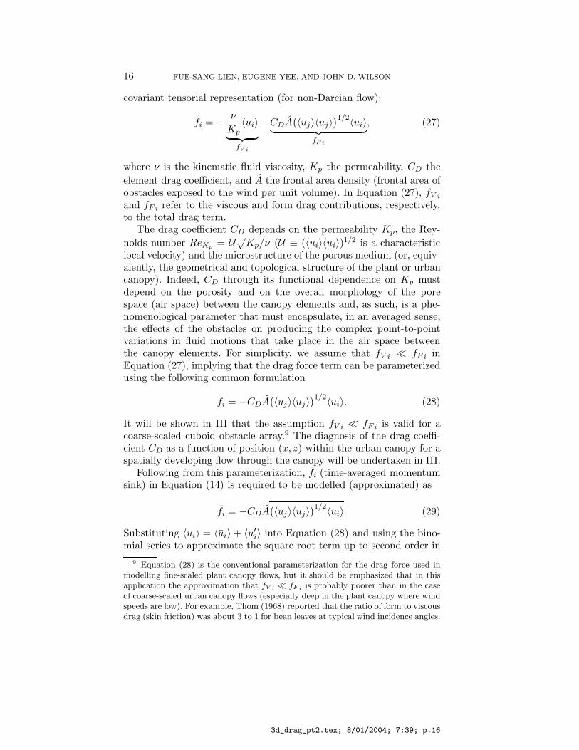
covariant tensorial representation (for non-Darcian flow):
fi = − ν
Kp〈ui〉
︸ ︷︷ ︸fV i
−CDA(〈uj〉〈uj〉
)1/2〈ui〉︸ ︷︷ ︸fF i
, (27)
where ν is the kinematic fluid viscosity, Kp the permeability, CD theelement drag coefficient, and A the frontal area density (frontal area ofobstacles exposed to the wind per unit volume). In Equation (27), fV i
and fF i refer to the viscous and form drag contributions, respectively,to the total drag term.
The drag coefficient CD depends on the permeability Kp, the Rey-nolds number ReKp = U
√Kp/ν (U ≡ (〈ui〉〈ui〉)1/2 is a characteristic
local velocity) and the microstructure of the porous medium (or, equiv-alently, the geometrical and topological structure of the plant or urbancanopy). Indeed, CD through its functional dependence on Kp mustdepend on the porosity and on the overall morphology of the porespace (air space) between the canopy elements and, as such, is a phe-nomenological parameter that must encapsulate, in an averaged sense,the effects of the obstacles on producing the complex point-to-pointvariations in fluid motions that take place in the air space betweenthe canopy elements. For simplicity, we assume that fV i fF i inEquation (27), implying that the drag force term can be parameterizedusing the following common formulation
fi = −CDA(〈uj〉〈uj〉
)1/2〈ui〉. (28)
It will be shown in III that the assumption fV i fF i is valid for acoarse-scaled cuboid obstacle array.9 The diagnosis of the drag coeffi-cient CD as a function of position (x, z) within the urban canopy for aspatially developing flow through the canopy will be undertaken in III.
Following from this parameterization, fi (time-averaged momentumsink) in Equation (14) is required to be modelled (approximated) as
fi = −CDA(〈uj〉〈uj〉
)1/2〈ui〉. (29)
Substituting 〈ui〉 = 〈ui〉 + 〈u′i〉 into Equation (28) and using the bino-
mial series to approximate the square root term up to second order in9 Equation (28) is the conventional parameterization for the drag force used in
modelling fine-scaled plant canopy flows, but it should be emphasized that in thisapplication the approximation that fV i fF i is probably poorer than in the caseof coarse-scaled urban canopy flows (especially deep in the plant canopy where windspeeds are low). For example, Thom (1968) reported that the ratio of form to viscousdrag (skin friction) was about 3 to 1 for bean leaves at typical wind incidence angles.
3d_drag_pt2.tex; 8/01/2004; 7:39; p.16

MATHEMATICAL FOUNDATION OF DRAG FORCE APPROACH 17
the velocity fluctuations 〈u′i〉 (or, equivalently, truncation of the Taylor
series expansion of the square root term at second order in the ex-pansion (order) parameter δ ≡ |〈u′
i〉|/(〈uj〉〈uj〉
)1/2),10 an approximateform for fi that is appropriate for time averaging can be derived as
fi ≈ −CDAQ
(〈ui〉 +
〈ui〉〈uj〉〈u′j〉
Q2+ 〈u′
i〉
+〈u′
i〉〈uj〉〈u′j〉
Q2+
〈ui〉〈u′j〉〈u′
j〉2Q2
)+ O(δ3), (30)
where Q ≡(〈ui〉〈ui〉
)1/2 is the magnitude of the spatially-averaged,time-mean wind speed.11
The approximation for fi in Equation (30) involves an orderly ex-pansion about a local, volume-averaged mean flow state 〈ui〉. The ex-pansion about this mean flow state suggests that the ratio of theturbulence kinetic energy to the mean flow kinetic energy is small
10 Strictly speaking, absolute convergence of the binomial series for the squareroot term requires that ∣∣∣∣
〈uj〉〈u′j〉
Q2+
κ
Q2
∣∣∣∣ <1
2,
where Q ≡(〈ui〉〈ui〉
)1/2. However, even if this condition is not satisfied, it is
nevertheless possible for the first few terms in the expansion of(〈uj〉〈uj〉
)1/2in
the putative small (order) parameter δ to be useful (viz., provide useful predictions)even though the expansion parameter is of order unity (which, strictly, will resultin the violation of the condition for absolute convergence of the binomial series).There are numerous examples of this phenomenon in other fields of endeavor: inquantum chromodynamics (QCD), the coupling constant for the strong interaction(force which holds the nucleus together) is large (αstrong ∼ 14) and the powerexpansion in the order parameter αstrong (perturbation theory) is not expected tobe reliable, yet the first few terms in perturbative calculations in QCD have beenfound surprisingly to give predictions that agree well with experimental results indeep electron-nucleon scattering reactions (Greiner and Schafer, 1994); and, theexpansion in small Reynolds number parameter for laminar flow around a cylinderis known to work well for Reynolds number of order 10 (Van Dyke, 1964).
11 An alternative procedure would have been to use the full infinite series (formal)expansion for the square root term, and then to assume Gaussian turbulence in thecanopy flow so that Wick’s theorem (Kleinert, 1990) can be applied to the time-averaged expansion to express all the higher-order velocity moments in terms ofonly various products of the second-order velocity moments. This produces an exactformal (albeit necessarily complicated) result for fi for the case of Gaussian turbu-lence, but is physically deficient since canopy turbulence is known to be stronglynon-Gaussian (Raupach et al., 1986). Furthermore, for strong turbulence whereδ = |〈u′
i〉|/Q ∼ O(1), the formal expansion of the square root term may not result in
a convergent series. Yet, the first few terms in this expansion may still neverthelesslead to useful results (see footnote 10).
3d_drag_pt2.tex; 8/01/2004; 7:39; p.17
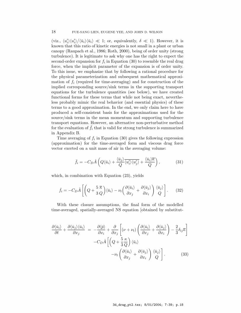
18 FUE-SANG LIEN, EUGENE YEE, AND JOHN D. WILSON
(viz., 〈u′i〉〈u′
i〉/〈ui〉〈ui〉 1; or, equivalently, δ 1). However, it is
known that this ratio of kinetic energies is not small in a plant or urbancanopy (Raupach et al., 1986; Roth, 2000), being of order unity (strongturbulence). It is legitimate to ask why one has the right to expect thesecond-order expansion for fi in Equation (30) to resemble the real dragforce, when the implicit parameter of the expansion is of order unity.To this issue, we emphasize that by following a rational procedure forthe physical parameterization and subsequent mathematical approxi-mation of fi (required for time-averaging) and for construction of theimplied corresponding source/sink terms in the supporting transportequations for the turbulence quantities (see below), we have createdfunctional forms for these terms that while not being exact, neverthe-less probably mimic the real behavior (and essential physics) of theseterms to a good approximation. In the end, we only claim here to haveproduced a self-consistent basis for the approximations used for thesource/sink terms in the mean momentum and supporting turbulencetransport equations. However, an alternative non-perturbative methodfor the evaluation of fi that is valid for strong turbulence is summarizedin Appendix B.
Time averaging of fi in Equation (30) gives the following expression(approximation) for the time-averaged form and viscous drag forcevector exerted on a unit mass of air in the averaging volume:
fi = −CDA
(Q〈ui〉 +
〈uj〉Q
〈u′i〉〈u′
j〉 +〈ui〉κ
Q
), (31)
which, in combination with Equation (23), yields
fi = −CDA
[(Q +
53
κ
Q
)〈ui〉 − νt
(∂〈ui〉∂xj
+∂〈uj〉∂xi
)〈uj〉Q
]. (32)
With these closure assumptions, the final form of the modelledtime-averaged, spatially-averaged NS equation [obtained by substitut-ing Equations (23), (26) and (32) into Equations (20) and (21)] becomes
∂〈ui〉∂t
+∂〈uj〉〈ui〉
∂xj= −∂〈p〉
∂xi+
∂
∂xj
[(ν + νt)
(∂〈ui〉∂xj
+∂〈uj〉∂xi
)− 2
3δijκ
]
−CDA
[(Q +
53
κ
Q
)〈ui〉
−νt
(∂〈ui〉∂xj
+∂〈uj〉∂xi
)〈uj〉Q
]. (33)
3d_drag_pt2.tex; 8/01/2004; 7:39; p.18
MATHEMATICAL FOUNDATION OF DRAG FORCE APPROACH 19
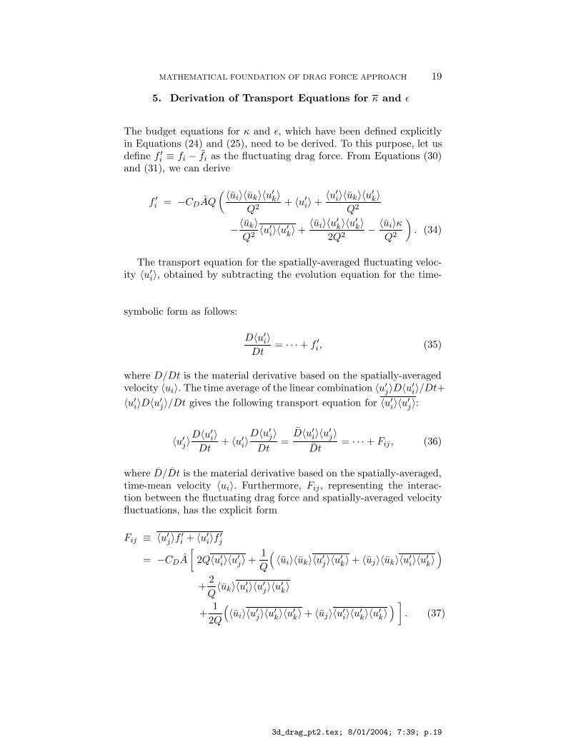
5. Derivation of Transport Equations for κ and ε
The budget equations for κ and ε, which have been defined explicitlyin Equations (24) and (25), need to be derived. To this purpose, let usdefine f ′
i ≡ fi − fi as the fluctuating drag force. From Equations (30)and (31), we can derive
f ′i = −CDAQ
(〈ui〉〈uk〉〈u′k〉
Q2+ 〈u′
i〉 +〈u′
i〉〈uk〉〈u′k〉
Q2
−〈uk〉Q2
〈u′i〉〈u′
k〉 +〈ui〉〈u′
k〉〈u′k〉
2Q2− 〈ui〉κ
Q2
). (34)
The transport equation for the spatially-averaged fluctuating veloc-ity 〈u′
i〉, obtained by subtracting the evolution equation for the time-averaged spatially-averaged velocity [Equation (20)] from the spatially-averaged Navier-Stokes equation [Equation (17)], can be written insymbolic form as follows:
D〈u′i〉
Dt= · · · + f ′
i , (35)
where D/Dt is the material derivative based on the spatially-averagedvelocity 〈ui〉. The time average of the linear combination 〈u′
j〉D〈u′i〉/Dt+
〈u′i〉D〈u′
j〉/Dt gives the following transport equation for 〈u′i〉〈u′
j〉:
〈u′j〉
D〈u′i〉
Dt+ 〈u′
i〉D〈u′
j〉Dt
=D〈u′
i〉〈u′j〉
Dt= · · · + Fij , (36)
where D/Dt is the material derivative based on the spatially-averaged,time-mean velocity 〈ui〉. Furthermore, Fij , representing the interac-tion between the fluctuating drag force and spatially-averaged velocityfluctuations, has the explicit form
Fij ≡ 〈u′j〉f ′
i + 〈u′i〉f ′
j
= −CDA
[2Q〈u′
i〉〈u′j〉 +
1Q
(〈ui〉〈uk〉〈u′
j〉〈u′k〉 + 〈uj〉〈uk〉〈u′
i〉〈u′k〉)
+2Q〈uk〉〈u′
i〉〈u′j〉〈u′
k〉
+1
2Q
(〈ui〉〈u′
j〉〈u′k〉〈u′
k〉 + 〈uj〉〈u′i〉〈u′
k〉〈u′k〉) ]
. (37)
3d_drag_pt2.tex; 8/01/2004; 7:39; p.19

20 FUE-SANG LIEN, EUGENE YEE, AND JOHN D. WILSON
One-half the trace of Fij yields
F ≡ 12Fii = 〈u′
i〉f ′i
= −CDA
[2Qκ +
1Q
(〈ui〉〈uk〉〈u′
i〉〈u′k〉)
+3
2Q
(〈uk〉〈u′
i〉〈u′i〉〈u′
k〉) ]
. (38)
The triple correlation term 〈u′i〉〈u′
i〉〈u′k〉 in Equation (38) can be
modelled, following Daly and Harlow (1970), as
〈u′i〉〈u′
i〉〈u′k〉 = 2Cs
κ
ε
[〈u′
k〉〈u′l〉
∂κ
∂xl+ 〈u′
i〉〈u′l〉
∂〈u′i〉〈u′
k〉∂xl
], (39)
where the closure constant Cs ≈ 0.3 is used in the present study.12 Thisis a gradient transport model for the third moments of the spatially-averaged fluctuating velocity and involves a tensor eddy viscosity. InEquations (38) and (39), the double correlation 〈u′
i〉〈u′j〉 was modelled
previously using the constitutive relationship in Equation (23).The transport equation for the time-averaged, resolved-scale kinetic
energy of turbulence κ is obtained by multiplying Equation (35) by 〈u′i〉
and time averaging the result. This procedure will give rise to the Fterm exhibited in Equation (38). This term represents the interactionof the flow with the obstacle elements and corresponds explicitly tothe work done by the turbulence against the fluctuating drag force.The term F can be interpreted as an additional physical mechanismfor the production/dissipation of κ associated with work against formand viscous drag on the obstacle elements. From this perspective, theexact transport equation for κ is
∂κ
∂t+ 〈uj〉
∂κ
∂xj= −∂Tj
∂xj− 〈u′
i〉∂
∂xj〈u′′
i u′′j 〉 +
(P + F
)− ε, (40)
where F ≡ 〈u′i〉f ′
i ; the flux Tj is
Tj ≡12〈u′
j〉〈u′i〉〈u′
i〉 + 〈u′j〉〈p′〉 − ν
∂κ
∂xj; (41)
and,
P ≡ −〈u′i〉〈u′
j〉∂〈ui〉∂xj
(42)
12 Alternatively, one can assume Gaussian turbulence in the canopy flow andsimply set this triple correlation (odd moment) to zero.
3d_drag_pt2.tex; 8/01/2004; 7:39; p.20
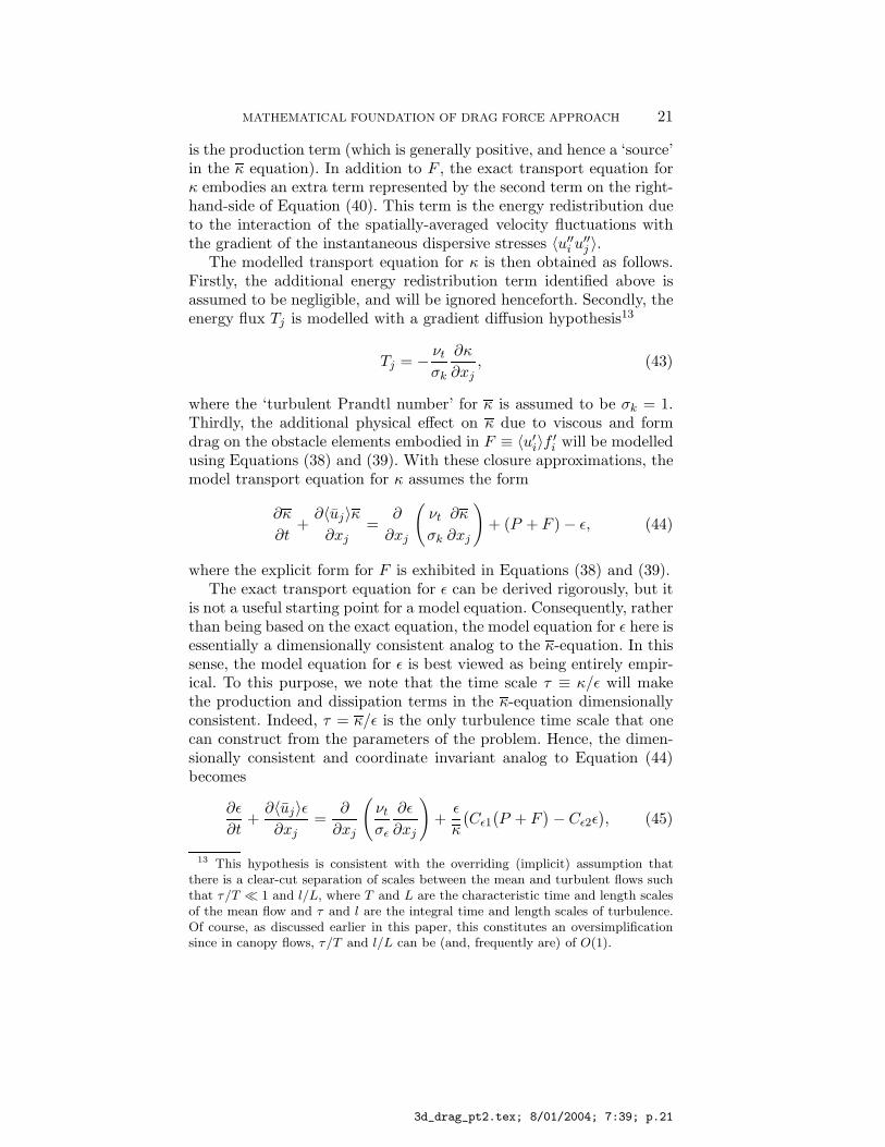
MATHEMATICAL FOUNDATION OF DRAG FORCE APPROACH 21
is the production term (which is generally positive, and hence a ‘source’in the κ equation). In addition to F , the exact transport equation forκ embodies an extra term represented by the second term on the right-hand-side of Equation (40). This term is the energy redistribution dueto the interaction of the spatially-averaged velocity fluctuations withthe gradient of the instantaneous dispersive stresses 〈u′′
i u′′j 〉.
The modelled transport equation for κ is then obtained as follows.Firstly, the additional energy redistribution term identified above isassumed to be negligible, and will be ignored henceforth. Secondly, theenergy flux Tj is modelled with a gradient diffusion hypothesis13
Tj = − νt
σk
∂κ
∂xj, (43)
where the ‘turbulent Prandtl number’ for κ is assumed to be σk = 1.Thirdly, the additional physical effect on κ due to viscous and formdrag on the obstacle elements embodied in F ≡ 〈u′
i〉f ′i will be modelled
using Equations (38) and (39). With these closure approximations, themodel transport equation for κ assumes the form
∂κ
∂t+
∂〈uj〉κ∂xj
=∂
∂xj
(νt
σk
∂κ
∂xj
)+ (P + F ) − ε, (44)
where the explicit form for F is exhibited in Equations (38) and (39).The exact transport equation for ε can be derived rigorously, but it
is not a useful starting point for a model equation. Consequently, ratherthan being based on the exact equation, the model equation for ε here isessentially a dimensionally consistent analog to the κ-equation. In thissense, the model equation for ε is best viewed as being entirely empir-ical. To this purpose, we note that the time scale τ ≡ κ/ε will makethe production and dissipation terms in the κ-equation dimensionallyconsistent. Indeed, τ = κ/ε is the only turbulence time scale that onecan construct from the parameters of the problem. Hence, the dimen-sionally consistent and coordinate invariant analog to Equation (44)becomes
∂ε
∂t+
∂〈uj〉ε∂xj
=∂
∂xj
(νt
σε
∂ε
∂xj
)+
ε
κ
(Cε1
(P + F
)− Cε2ε
), (45)
13 This hypothesis is consistent with the overriding (implicit) assumption thatthere is a clear-cut separation of scales between the mean and turbulent flows suchthat τ/T 1 and l/L, where T and L are the characteristic time and length scalesof the mean flow and τ and l are the integral time and length scales of turbulence.Of course, as discussed earlier in this paper, this constitutes an oversimplificationsince in canopy flows, τ/T and l/L can be (and, frequently are) of O(1).
3d_drag_pt2.tex; 8/01/2004; 7:39; p.21
22 FUE-SANG LIEN, EUGENE YEE, AND JOHN D. WILSON
where σε = 1.3, Cε1 = 1.44 and Cε2 = 1.92 are empirical (closure)constants. The ε-equation here essentially retains the same form as theusual model equation for ε commonly utilized in the standard k-ε model(Launder and Spalding, 1974). The only difference here is that the dragforce effect on the turbulence (embodied in the term F ) has been in-cluded with the production term P in Equation (45). The ε productionterm is modelled as Cε1P/τ [P is determined through Equation (42)on substitution of Equation (23)] in the relaxation time approximation.Finally, the destruction of dissipation term has a simple physical inter-pretation in terms of a relaxation time; namely, Cε2ε
2/κ = Cε2ε
/τ , with
τ in this context identified as the lag in the dissipation ε, correspond-ing to the time it will take energy injected (produced) at the energycontaining wavenumbers to be reduced to the size of the dissipativewavenumbers.
In Equation (45), we have grouped F with P in the ε-equation.In other words, we sensitize the ε-equation to the effects of form andviscous drag of the obstacle elements by replacing P with P + F inthe ‘production of dissipation’ term (usually, the effect of the obstacleelements is to enhance the dissipation in the canopy airspace). Thistreatment is similar to the rationale used by Ince and Launder (1989)for dealing with buoyancy effects on turbulence in buoyancy-drivenflows. In these types of flows, the gravitational production term G ≡−βgiu′
iT′ (gi is the gravitational acceleration vector, β is the thermal
expansion coefficient, and T ′ is the virtual temperature fluctuation) isincluded with P in the transport equation for the viscous dissipationrate. In this regard, our proposed approach for treating F in the ε-equation differs from that suggested by Getachew et al. (2000).14
6. Whither Wake Production
The closure of the spatially-averaged RANS equation [cf. Equations (12)and (13)] requires a transport equation for 〈k〉 ≡ 1
2〈u′iu
′i〉 (i.e., the
spatially-averaged turbulence kinetic energy), whereas that for the time-averaged spatially-averaged NS equation [cf. Equations (20) and (21)]requires a transport equation for κ ≡ 1
2〈u′i〉〈u′
i〉 (i.e., the time-averagedresolved-scale kinetic energy of turbulence). The model transport equa-tion for κ in Equation (44) included a source/sink term F whose form
14 In general, the dissipation rate model (or, equivalently, other forms of the scale-determining equation) is the weakest link in turbulence modelling of complex flows,whether it be for two-equation turbulence models or for Reynolds stress transportmodels. Although more sophisticated dissipation models have been developed, theyseem to lack the general applicability of the simple model used here.
3d_drag_pt2.tex; 8/01/2004; 7:39; p.22
MATHEMATICAL FOUNDATION OF DRAG FORCE APPROACH 23
can be systematically derived in terms of the drag force term thatappears in the mean momentum equation [cf. Equations (38) and (39)].
The budget equation for 〈k〉 can be derived by applying the spatialaveraging operator to the standard transport equation for k to give
∂〈k〉∂t
+ 〈uj〉∂〈k〉∂xj
= −〈u′iu
′j〉
∂ui
∂xj
− ∂
∂xj
12〈u′
ju′iu
′i 〉 + 〈u′
jp′ 〉 +
12〈 u′′
j u′iu
′i 〉
︸ ︷︷ ︸I
+ν∂2〈k〉∂x2
j
− ε −⟨
u′iu
′j
′′ ∂u′′i
∂xj
⟩
︸ ︷︷ ︸II
. (46)
In Equation (46), ε ≡ ν⟨∂u′
i∂xj
∂u′i
∂xj
⟩is the isotropic turbulent dissipation
rate for 〈k〉.The transport equation for 〈k〉 contains two additional terms (des-
ignated I and II) that need to be approximated. Term I correspondsto the dispersive transport of 〈k〉 [analogous to the dispersive flux ofmomentum in Equations (12) and (13)]. Term II can be identified as awake production term (see Raupach and Shaw, 1982) which accountsfor the conversion of mean kinetic energy to turbulent energy in theobstacle wakes by working of the mean flow against the drag. This termis analogous to the F term that appears in the transport equation forκ, but unlike F whose form can be systematically derived from theform and viscous drag force term that appears in the mean momentumequation, the link (if any) between the wake production term in Equa-tion (46) and the drag force term in the mean momentum equationis less obvious. For example, Raupach and Shaw (1982) showed thatprovided (1) the dispersive stress 〈u′′
i u′′j 〉 and the dispersive transport of
〈k〉 are both negligible and (2) the mean kinetic energy is not directlydissipated to heat in the canopy, the wake production term can beapproximated as follows:
−⟨(u′
iu′j)
′′ ∂u′′i
∂xj
⟩= −〈ui〉fi = 2CDAQ
(12〈ui〉〈ui〉
)
︸ ︷︷ ︸K
, (47)
where K represents the mean kinetic energy (kinetic energy of thespatially-averaged time-mean flow). Note that use of Equation (47) asa model for the wake production term strictly provides a source termin the transport equation for 〈k〉 and, physically, corresponds to the
3d_drag_pt2.tex; 8/01/2004; 7:39; p.23

24 FUE-SANG LIEN, EUGENE YEE, AND JOHN D. WILSON
conversion of mean kinetic energy (MKE) to turbulence kinetic energy(TKE) [MKE → TKE which here is equated simply to the work doneby the flow against form drag −〈ui〉fi].
Generally, the inclusion of the wake production term of Equation (47)in the transport equation for 〈k〉 has been found to result in an overesti-mation of the turbulence level within a vegetative canopy. For example,Wilson and Shaw (1977) included a wake production term in theirstreamwise normal stress equation and found that their model over-estimated the streamwise and vertical turbulence intensities in a corncanopy despite the fact that they tuned their mixing length. Further-more, Wilson (1985) found that a zone of reduced TKE (“quiet zone”)in the near lee of a shelter belt cannot be reproduced correctly withthe inclusion of a wake production term in the normal stress transportequations15 but, rather, required the exclusion of this source term cou-pled with the inclusion of a sink term corresponding approximately toEquation (31). Likewise, Green (1992) and Liu et al. (1996) found thatit was necessary to include also a sink term in the budget equation for〈k〉 and, to this purpose, modelled the “wake” production term in thebudget equation for 〈k〉 in an ad hoc manner as
−⟨(u′
iu′j)
′′∂u′′i
∂xj
⟩= βP CDAQ
(12〈ui〉〈ui〉
)
︸ ︷︷ ︸K
−βdCDAQ
(12〈u′
iu′i〉)
︸ ︷︷ ︸〈k〉
, (48)
which includes a gain to 〈k〉 from conversion of the mean kinetic en-ergy K to turbulence energy at the larger scales (source term) anda loss from 〈k〉 of the large-scale turbulence energy to smaller (wake)scales (sink term). In Equation (48), βP and βd are O(1) empiricaldimensionless constants with no particular physical significance. Morespecifically, Green (1992) argued heuristically that the sink term inEquation (48) was required to account for the accelerated cascade of 〈k〉from large to small scales due to the presence of the roughness elements(arising from the rapid dissipation of fine-scale wake eddies in a plantcanopy). Liu et al. (1996) in their 〈k〉 equation used βP = 2 and βd = 4,generally giving a model where the overall effect of the “source” termin Equation (48) is to act as a sink term within the canopy. Indeed, Liuet al. (1996) noted that the ad hoc inclusion of the sink term (secondterm on the right-hand side) of Equation (48) [which was inserted inhindsight] was important, for otherwise they found that their predicted
15 The inclusion of a wake production (source) term generally led to an increaseof the TKE level in the near lee of a porous barrier, contrary to the availableexperimental observations.
3d_drag_pt2.tex; 8/01/2004; 7:39; p.24
MATHEMATICAL FOUNDATION OF DRAG FORCE APPROACH 25
〈k〉 was “about 100% larger than the experimental measurements whenthe second term was ignored”.
Sanz (2003) described an alternative method for the determinationof the source model coefficients βP and βd in Equation (48). Sanz recog-nized the confusion that had reigned for some time as to the ‘correct’source terms in TKE and dissipation-rate equations for canopy flow.His solution was to constrain particular pre-existing (and heuristic)expressions for the forms of the sinks Sk and Sε in the model equationsfor TKE (“k”) and its dissipation rate ε, though without identifying kspecifically with 〈k〉 or with κ (i.e., a precise interpretation of k wasnot provided). The constraints emerged by requiring that the k-ε model(with these sources) should reproduce an exponential mean wind profilein the canopy layer, in the special case of a horizontally-uniform, neutralplant canopy flow in which both leaf area density and the effective tur-bulence lengthscale k3/2
/ε were (by requirement) height independent.
Evidently, this approach does not offer the generality provided here.In contrast, the additional source/sink term F that appears in the
budget equation for κ can be systematically derived from rate of work-ing of the turbulent velocity fluctuations against the fluctuating dragforce, and appears naturally in the derivation of the budget equationfor κ. The form of the source/sink term F results from a series ex-pansion for fi that is truncated systematically at second order in thevelocity fluctuations 〈u′
i〉. All constants in this model for F are derivedexplicitly from the expansion procedure; no adjustable constants ariseand no additional ad hoc modifications are applied to F , in contrast tothe mentioned treatments of the transport equation for 〈k〉 [cf. Equa-tion (48)]. Even though the ‘turbulence kinetic energy’ κ ≡ 1
2〈u′i〉〈u′
i〉(time-averaged, resolved-scale kinetic energy of turbulence) used inour turbulence closure model is different from the usual form of thespatially-averaged turbulence kinetic energy 〈k〉 ≡ 1
2〈u′iu
′i 〉, they are
nevertheless related as follows:
〈k〉 − κ =12(〈u′′
i u′′i 〉 − 〈u′′
i u′′i 〉)
=12〈 (u′
i)′′(u′i)′′ 〉. (49)
Note that the difference between 〈k〉 and κ is proportional to thedifference between the two forms of dispersive stress that appear in thespatially-averaged RANS equation and the time-averaged, spatially-averaged NS equation. However, note that this difference can be ex-pressed as the spatial average of time averages of the departures ofvelocity fluctuations from their spatial (volume) average. Since thisterm involves a “perturbation of a perturbation”, it seems reasonable
3d_drag_pt2.tex; 8/01/2004; 7:39; p.25

26 FUE-SANG LIEN, EUGENE YEE, AND JOHN D. WILSON
to assume16 that
0 ≈ 12∣∣ ⟨(u′
i)′′(u′i)′′⟩ ∣∣ max
(〈k〉, κ
). (50)
With this assumption, 〈k〉 and κ are expected to be almost equal invalue (viz., 〈k〉 ≈ κ). This, together with Equation (22), implies that
〈u′′i u
′′j 〉 ≈ 〈u′′
i u′′j 〉, (51)
or, in other words, the dispersive stresses are expected to be approx-imately equal to the spatial average of the high-frequency turbulentstresses. Finally, with reference to Equation (22), this also implies that〈u′
i〉〈u′j〉 ≈ 〈u′
iu′j 〉. The latter approximation will be used in III to
compare model predictions of 〈u′i〉〈u′
j〉 with the diagnosed values of〈u′
iu′j 〉 obtained from a high-resolution RANS simulation.
Interestingly, the ‘zeroth-order’ term in our expansion of F in Equa-tion (38), rewritten below
F ≡ 〈u′i〉f ′
i = −2CDAQ
(12〈u′
i〉〈u′i〉)
︸ ︷︷ ︸κ
+H.O.T, (52)
where H.O.T denotes higher-order correction terms, is analogous to thesink term contribution for the wake production term in the Liu et al.(1996) model of Equation (48) [except the factor here is 2, rather thanβd = 4]. Note that the higher-order correction terms for F can haveeither sign implying that they are source/sink terms. More importantly,it needs to be emphasized that the leading-order term of F is a sinkterm, and not a source term implying that in the transport equationfor κ the conversion of MKE to TKE is ipso facto absent.17 In thissense, the transport equation derived here for κ is reminiscent of thetransport equation for shear kinetic energy (SKE) originally proposedby Wilson (1988). Wilson formulated a heuristic approach in which
16 No experimental observations are available to support or refute this assumption.It is conceivable that large-eddy simulations (LES) of plant or urban canopy flowsmay provide “data” that can be used to evaluate the validity of this assumption.
17 Although Wang and Takle (1995b) use the transport equation for κ for theirsimulations of flows near shelter belts, they seem to have incorporated wrongly a
source term SMKE ≡ CDA(〈ui〉〈ui〉
)3/2in the κ-equation representing MKE con-
version to κ by drag of the shelter belt on the flow. Equation (52) shows that theinclusion of the MKE conversion term in the κ-equation is not self-consistent withthe momentum sink terms introduced into the transport equations for the time-averaged spatially-averaged mean wind. Furthermore, Wilson and Mooney (1997)reported that using the source term SMKE in the κ transport equation resulted in adrastic overestimation of peak TKE levels near the porous barrier.
3d_drag_pt2.tex; 8/01/2004; 7:39; p.26
MATHEMATICAL FOUNDATION OF DRAG FORCE APPROACH 27
he partitioned the turbulence energy into two spectral bands; namely,bands of turbulent motion corresponding to the large-scale or shearkinetic energy and to small-scale or wake kinetic energy (WKE). In thisapproach, the MKE conversion due to the drag forces was assumed tobe re-deposited as fine-scale WKE [viz., in small eddies on the scale ofthe canopy elements (twigs, leaves, etc.) in the fine-scaled plant canopy]where it was rapidly dissipated as heat. The conversion of SKE to WKEwas modelled here simply as the sum of two terms, the first representingthe conventional dissipation due to the vortex-stretching mechanismand the second arising from the rate of working of turbulence againstthe vegetation drag resulting in an additional sink term in the SKEtransport equation of the form
εfd = 2CDA〈u〉(〈u′2〉 +
12〈v′2〉 +
12〈w′2〉
). (53)
Note that the sink term εfd appearing in the SKE transport equationis very similar to the leading order term of F (sink term) appearing inthe κ transport equation [cf. Equation (52) with Equation (53)], themathematical difference being solely due to Wilson’s approximationthat u
√u2 + v2 + w2 ≈ u2 (etc.). However the mathematical similarity
should not cause one to lose sight of the important logical difference, forWilson’s instantaneous velocity (u, v, w) lacked the proper designationas a spatial average.
Despite the outward similarities between the current treatment ofκ and Wilson’s treatment of SKE, it is legitimate to ask whether κ isexactly coincident with SKE defined by Wilson. The implicit assump-tion in Wilson’s (1988) two-band “spectral division” for the turbulenceenergy resides in the presumption that there is a clear cut separationbetween the large (SKE) and small (WKE) scale components of theturbulence and that MKE and large-scale TKE lost due to the actionof form drag must necessarily be re-deposited as fine-scale, rapidlydissipated eddies in the WKE component. In this two-band spectraldecomposition approach, the characteristic length scale separating thelarge- and small-scale components of turbulence is a physical scaleimposed by the elements of the fine-scaled plant canopy itself (viz.,direct interaction of the flow with the foliage imposes a new, smallerlength scale on the flow corresponding to the leaf or twig scale, and it isthis range of scales which is associated with the fine-scale WKE). Whilethe decomposition of the turbulence into a large-scale SKE and fine-scale WKE is reasonable for a fine-grained (and dense) plant canopy,it appears to be less appropriate for a coarse-grained urban canopywhere the wake scales of motion behind buildings (element wakes) are
3d_drag_pt2.tex; 8/01/2004; 7:39; p.27

28 FUE-SANG LIEN, EUGENE YEE, AND JOHN D. WILSON
not small, but rather frequently comparable to the scales associatedwith the shear production of turbulence energy.
We note that κ ≡ 12〈u
′i〉〈u′
i〉 (time-mean locally-spatially-filtered tur-bulence kinetic energy) represents a restricted spectrum of turbulentmotions and, in this sense, is similar to SKE defined by Wilson (1988).However, the basic difference in κ and SKE arises from the fact that theimplicit scale separating “large” and “small” scales of turbulent motionin κ is obtained from the application of an explicit spatial filtering(volume-averaging) on the turbulent velocity fluctuations u′
i itself [incontrast to SKE where the separation between large and small scalesof motion devolves from a physical length scale imposed on the flowby the canopy elements (e.g., fine-grained foliage in a plant canopy)].Furthermore, the scale separating large and small turbulent motions inthe two-band spectral representation of Wilson (1988) is not explicitlyspecified, other than stating it is to guarantee that the SKE excludes theTKE residing in the fine wake scales. In contrast, the scale separatinglarge and small turbulent motions in the definition of κ is explicitlyspecified by the filter width ∆ that defines the spatial filter applied tothe turbulent velocity fluctuations [cf. Equations (1) and (4)].
To explore this concept further, it is informative to write κ in termsof the following spectral representation:
κ ≡ 12〈u′
i〉〈u′i〉 =
12
∫ ∞
−∞
∣∣G(k)∣∣2Φ(k)dk, (54)
where k is the wavenumber vector and Φ(k) is the turbulence energyspectral density defined over the entire spectrum of turbulent motions.In Equation (54), G(k) is the Fourier transform of the top-hat filterexhibited in Equation (4) given by
G(k) =3∏
i=1
sin(∆(i)k(i)
/2)
∆(i)k(i)
/2
, (55)
where ki is the i-th component of the wavenumber vector k, ∆i is thefilter width in the xi-direction (with total filter width ∆ specified by∆ = V 1/3 =
(∆1∆2∆3
)1/3), and the round parentheses around anindex i [viz., (i)] indicates that there is no summation over i for thisrepeated index. Equation (54) shows explicitly that κ only incorporatesthe turbulence energy in a low wavenumber band with wavenumbercontributions confined largely to the range |k| . π/∆ determinedby the transfer function
∣∣G(k)∣∣2 of the spatial filter defined in Equa-
tion (4). This spatial filter effectively removes (attenuates) small-scaleflow features that are less than an externally introduced (imposed)length scale ∆ (filter width). However, we emphasize that this spatial
3d_drag_pt2.tex; 8/01/2004; 7:39; p.28
MATHEMATICAL FOUNDATION OF DRAG FORCE APPROACH 29
filtering operation on the velocity field does not introduce a clear-cutseparation between resolved and sub-filter scales because (1) the top-hat filter allows a frequency overlap between the resolved and sub-filterscales and (2) the turbulence energy spectrum is continuous so thatthe smallest resolved scales of motion are close to those of the largestsub-filter scales of motion.
The time-average of the spatially-averaged NS equations leads logi-cally to the consideration of the transport equation for κ, rather than〈k〉. This averaging scheme results naturally in a two-band spectralrepresentation for the TKE that is similar to that proposed by Wilson(1988). However, while the dual-band model of Wilson partitions theturbulence energy into a large-scale SKE and fine-scale WKE with thelength scale separating these two bands determined by the scale of theindividual canopy elements (e.g., leaf and twig scale in a plant canopy),the dual-band model here is perhaps interpreted best as partitioningthe turbulence energy into a resolved scale and sub-filter scale bandwith the separation between these two scales externally imposed bythe filter width ∆ of the spatial filter applied in the averaging oper-ation. In this interpretation, κ should be identified with the resolvedturbulence kinetic energy (TKE [> ]) that is due to energetic motionsin the flow at scales greater than the externally determined lengthscale ∆ (filter width). A key aspect of the modelled transport equationfor κ ≡ TKE [ > ] [cf. Equation (44)] is the exchange or conversion ofkinetic energy between TKE [> ] and the kinetic energy of turbulentmotions at scales less than ∆ (TKE [< ]). The leading-order term inF is negative, implying a “forward scatter” of TKE [> ] into TKE [< ],a physical mechanism which reduces the level of TKE [> ]. More sig-nificantly, the leading-order term of F does not involve a source termrelated to the conversion of MKE to TKE [> ]. However, higher-orderterms of F may possibly embody an increase of the level of TKE [> ]
due to interactions between the time-mean spatially-averaged meanflow and the resolved-scale turbulence.18
Applying a spatial filter to the equations of motion results in a reduc-tion in the complexity and information content of the flow, but intro-duces a length scale into the description of the fluid dynamics, namelythe width ∆ of the filter used. Assuming that the filter width appliedis within the inertial range of scales of fluid motion, the application ofthe spatial filter will cause the turbulence kinetic energy wavenumber
18 The sign of many of the higher-order terms in F is indefinite, so some ofthese interactions between the mean flow and the resolved-scale turbulence (viz.,turbulent motions with length scales larger than the filter width ∆, or equivalentlywith wavenumbers |k| . π
/∆) may be sink terms that contribute to the reduction
of TKE [ > ].
3d_drag_pt2.tex; 8/01/2004; 7:39; p.29

30 FUE-SANG LIEN, EUGENE YEE, AND JOHN D. WILSON
spectrum in three dimensions of the filtered turbulent motions to roll-off rapidly below the length scale ∆ as |k|−2−5/3 [cf. Equations (54)and (55)], instead of continuing at the slower Kolmogorov scaling law,|k|−5/3. This roll off shortens the inertial range for the spatially-filteredvelocity field, resulting in a reduction in the energy associated with thehigher wavenumbers in the filtered velocity and an increased dissipationin the range of scales |k|∆ π, implying an increased drain of theenergy of the resolved (large) scales by those of the sub-filter (small)scales. The effects of the small-scale fluid motions on the resolved ener-getics of turbulence in the canopy flow (embodied in κ) must physicallybe described by an increased (effective) “viscous” dissipation εeff ofthe resolved scales of motion that now becomes effective at |k|∆ ≈ π(rather than at the larger wavenumber associated with the Kolmogorovmicroscale), with εeff consisting of two basic contributions: namely,the conventional free-air dissipation associated with the spectral eddycascade and an additional dissipation (≈ 2CDAQκ) devolving fromair/obstacle interactions that result in additional source/sink termsin the κ-equation after a spatial filtering operation has been explic-itly applied to the instantaneous velocity fluctuations. The effect ofthis additional dissipation is embodied in the leading-order term of F[cf. Equation (52)].
7. Conclusions
In this paper, we showed how a modified k-ε model for the prediction ofthe time-mean spatially averaged wind and turbulence fields in a canopycan be derived ‘sytematically’ (or, at least in a self-consistent manner)by time-averaging the spatially-averaged NS equation. This procedureensures the mathematical and logical consistency of parameterizationof source/sink terms in the mean momentum equations and in thesupporting transport equations for κ and ε. Given a parameterizationfor the momentum source/sink fi in the spatially-averaged NS equationthat represents the effects of the form and viscous drag in the urbancanopy on the flow, a series expansion is applied to this term with atruncation at the second order in the velocity fluctuations 〈u′
i〉. Trun-cation at this order produces a quadratically nonlinear model for thetime-averaged momentum sink fi, and also permits the correspondingsource/sink term in the transport equation for κ to be methodicallyobtained.
The current approach of time-averaging the spatially-averaged NSequations is logically (and self-consistently) linked with the transportequation for κ (time-averaged, resolved-scale kinetic energy of turbu-
3d_drag_pt2.tex; 8/01/2004; 7:39; p.30

MATHEMATICAL FOUNDATION OF DRAG FORCE APPROACH 31
lence), rather than that for 〈k〉 (spatially-averaged turbulence kineticenergy). Interestingly, κ very explicitly and naturally does not includeTKE at scales smaller than the filter width ∆ = V 1/3. In this sense,κ here is similar to SKE considered by Wilson (1988). The basic dif-ference in κ and SKE arises from the fact that the small length scaleimposed on the flow by the individual canopy elements (e.g., individualleaves) is the characteristic scale that is used (implicitly) in Wilson’sapproach to distinguish the large scales associated with SKE with thesmall scales associated with WKE, whereas in the present approachan externally imposed filter width ∆ is used to distinguish between theresolved scales associated with κ and the kinetic energy associated withthe sub-filter (unresolved) scales. The current approach seems moreapplicable to coarse-scaled cuboid arrays where the wake scales of theindividual canopy elements are not necessarily small in comparison tothe scales associated with the shear production. With this distinction,the present approach can be interpreted as providing a formal basis forWilson’s dual-band spectral decomposition of the TKE [viz., we haveprovided a precise mathematical formulation of the heuristic ideas for“spectral division” of the TKE sketched earlier by Wilson (1988) forparameterizing turbulence in RANS models which treat the interactionof the wind with obstacles using a distributed momentum sink in themean momentum equations].
Appendix A: Dispersive Stress Tensor Model
While there currently exists no reference data to guide the modellingof the ‘conventional’ dispersive stress tensor 〈ui
′′uj′′〉, it is nevertheless
possible to construct a structural model for this quantity as follows. Tobegin, consider the Reynolds equation for mean momentum conserva-tion in a neutrally buoyant flow that obtains at any point in the canopyairspace:
∂ui
∂t+
∂(ujui
)
∂xj+
∂p
∂xi+
∂u′iu
′j
∂xj− ν
∂2ui
∂x2j
= 0. (56)
After applying the volume-averaging operator of Equation (5) to Equa-tion (56), the dispersive stress 〈ui
′′uj′′〉 arises from the noncommu-
tation of the product operator and the volume-averaging operator inthe nonlinear convective term. In view of this, to construct a struc-tural model for the dispersive stress we consider a simplification ofthe nonlinear convective term of Equation (56) that is obtained by
3d_drag_pt2.tex; 8/01/2004; 7:39; p.31
32 FUE-SANG LIEN, EUGENE YEE, AND JOHN D. WILSON
volume-averaging (smoothing) the advection velocity; viz., replacingthe nonlinear convective term in Equation (56) by 〈uj〉∂ui
/∂xj to give
∂ui
∂t+
∂(〈uj〉ui
)
∂xj+
∂p
∂xi+
∂u′iu
′j
∂xj− ν
∂2ui
∂x2j
= 0. (57)
In Equation (57), the time-mean velocity ui is advected by a smoothedvelocity 〈uj〉 obtained by volume averaging. Replacing the advectionvelocity uj by 〈uj〉 simplifies the problem by reducing the nonlineareffects of the convective term.
The spatially filtered time-mean fluid velocity 〈ui〉 is related to thetime-mean fluid velocity ui as 〈ui〉 = G ? ui, where G is an operatorwhose Green’s function is the filter defined by Equations (1) and (4).The “inverse” is denoted by ui = G−1 ? 〈ui〉, assuming that a formalinverse G−1 of G exists. Using this terminology, Equation (57) [simpli-fied RANS equation with the degree of nonlinearity of the convectiveterm reduced] can be written more informatively as follows:
∂(G−1 ? 〈ui〉
)
∂t+
∂(〈uj〉ui
)
∂xj+
∂(G−1 ? 〈p〉
)
∂xi
+∂(G−1 ? 〈u′
iu′j〉)
∂xj− ν
∂2(G−1 ? 〈ui〉
)
∂x2j
= 0. (58)
Applying the spatially-averaging operator G? to Equation (58) givesexplicitly
∂〈ui〉∂t
+∂(〈uj〉〈ui〉
)
∂xj+
∂〈p〉∂xi
+∂〈u′
iu′j〉
∂xj− ν
∂2〈ui〉∂x2
j
=
−[
G?,∂
∂t
]ui +
∂
∂xj
(〈ui〈uj〉〉 − 〈ui〉〈uj〉
)
+
[G?,
∂
∂xj
]P(ui, 〈uj〉
)+[G?,
∂
∂xi
]p
+
[G?,
∂
∂xj
](u′
iu′j
)−[G?,
∂
∂xj
](ν
∂ui
∂xj
), (59)
where P (f, g) ≡ fg is the product operator.Now, in view of the spatial averaging theorem of Equation (2) used
with G specified by Equation (4), most of the terms on the right-hand side of Equation (59) vanish on application of the no-slip andimpermeability conditions on the velocity field at the surfaces of theobstacles inside the averaging volume V . The non-vanishing terms
3d_drag_pt2.tex; 8/01/2004; 7:39; p.32

MATHEMATICAL FOUNDATION OF DRAG FORCE APPROACH 33
involving the commutator brackets on the right-hand side of Equa-tion (59) are −
[G?, ∂
/∂xi
]p and
[G?, ∂
/∂xj
](ν∂ui
/∂xj
)which in view
of Equation (14) can be identified physically with, respectively, fFi
and fV i (namely, the form and viscous drag force vectors exerted on aunit mass of air in the averaging volume). Noting that fi = fFi + fV i,Equation (59) simplifies to the following form
∂〈ui〉∂t
+∂(〈uj〉〈ui〉
)
∂xj+
∂〈p〉∂xi
+∂〈u′
iu′j〉
∂xj− ν
∂2〈ui〉∂x2
j
=
− ∂
∂xj
(〈ui〈uj〉〉 − 〈ui〉〈uj〉
)+ fi, (60)
which on comparison with Equations (12) and (13) implies the followingstructural model for the dispersive stress tensor expressed in terms ofthe spatially-averaged time-mean velocity 〈ui〉:
〈u′′i u
′′j 〉 = 〈ui〈uj〉〉 − 〈ui〉〈uj〉
=⟨(
G−1 ? 〈ui〉)〈uj〉
⟩−〈ui〉〈uj〉. (61)
Note that the model for 〈u′′i u
′′j 〉 in Equation (61) is derived directly from
a regularized form of the RANS equation, and as such, is consistentwith various transformation symmetries (e.g., Galilean invariance, timeinvariance, etc.) of this equation. Furthermore, the model for 〈u′′
i u′′j 〉
does not involve any model (closure) coefficients and suggests thatthe implied dispersive stress model must necessarily involve an explicitfiltering and an inversion operation. Finally, in light of Equations (49),(50), and (51), the structural model for 〈u′′
i u′′j 〉 can also be used as a
model for 〈u′′i u
′′j 〉.
To implement the model for 〈u′′i u
′′j 〉, we are required to construct an
approximation for the inverse operator G−1 (which in view of Equa-tion (4) is the inverse operator for the volume-averaging operation).To proceed with this construction, consider the top-hat filter of Equa-tion (4) applied in a single direction (say, the x-direction) only. Nowperform a Taylor series expansion of a flow quantity φ(y) about thefixed point x to give
φ(y) =∞∑
n=0
1n!(y − x
)n ∂nφ(x)∂xn
(62)
and insert this expansion into the one-dimensional version of Equa-tion (1) to give
〈φ〉(x) =∞∑
n=0
α(n)
n!∂nφ(x)
∂xn(63)
3d_drag_pt2.tex; 8/01/2004; 7:39; p.33
34 FUE-SANG LIEN, EUGENE YEE, AND JOHN D. WILSON
where α(n) denotes the n-th order moment of the convolution kernel G:
α(n) ≡ (−1)n∫ ∞
−∞snG(s) ds. (64)
For a symmetric filter considered here, all odd moments vanish (viz.,α(n) = 0 for n odd). Equation (63) shows that we can approximate thespatial filtering operation by truncating the Taylor series expansion to(N +1) terms to give a filtering operation that is defined by a low-orderdifferential filter:
〈φ〉(x) ≈N∑
n=0
α(n)
n!∂nφ(x)
∂xn. (65)
The unfiltered flow quantity φ can be expressed formally as
φ(x) ≈(
N∑
n=0
α(n)
n!∂n
∂xn
)−1
〈φ(x)〉. (66)
A simple explicit approximation of the inverse operator for N = 2(valid to second order in the filter width ∆x) can be written as [using aformal Taylor series expansion for the inverse operator of Equation (66)valid to second order]
φ(x) ≈(
1 − ∆2x
24∂2
∂x2
)〈φ(x)〉, (67)
where 1 is the identity operator. In Equation (67), we have used thefact that α(2) = ∆2
x
/12 for a one-dimensional top-hat filter with filter
width ∆x. The inversion operator in three-dimensions can be obtainedfrom composing three one-dimensional filters to give approximately
φ(x) ≈(
1 − ∆2x
24∂2
∂x2−
∆2y
24∂2
∂y2− ∆2
z
24∂2
∂z2
)〈φ(x)〉
≡ H∆(〈φ(x)〉
), (68)
where H∆ denotes the Helmholtz operator with ∆ ≡(∆x∆y∆z
)1/3
being the effective filter width in three dimensions.
Appendix B: Non-perturbative Evaluation of Source Terms
The calculation of fi and F described in Sections 4 and 5 was basedon expanding the spatially filtered total instantaneous velocity ampli-tude
(〈uj〉〈uj〉
)1/2 using the binomial series and time averaging the
3d_drag_pt2.tex; 8/01/2004; 7:39; p.34

MATHEMATICAL FOUNDATION OF DRAG FORCE APPROACH 35
various terms in this expansion. However, the convergence of this se-ries required that the time-averaged resolved scale kinetic energy ofturbulence be sufficiently small compared to the magnitude of thespatially-averaged time-mean wind speed such that the condition forabsolute convergence of the binomial series (see footnote 10) is satisfied.It is conceivable that this condition for absolute convergence of thebinomial series is violated in a canopy flow for cases of strong turbu-lence where 〈u′
j〉〈u′j〉 & 〈uj〉〈uj〉. This appendix offers an alternative
method (based on a non-perturbative approach) for the calculationof fi and F that is valid for the case of strong turbulence (and, alsofor weak turbulence of course). The actual calculation method for thenon-perturbative evaluation of fi and F is quite complex, but themethodology is generally applicable and does not require the existenceof a small expansion parameter δ ≡
∣∣〈u′i〉∣∣/Q [cf. Equation (30)].
To begin, recall that
fi ≡ −CDA(〈uj〉〈uj〉
)1/2〈ui〉
= −CDA(〈uj〉〈uj〉
)1/2(〈ui〉 + 〈u′i〉)
(69)
and
F ≡ 〈u′i〉f ′
i
= −CDA
(〈ui〉
(〈uj〉〈uj〉
)1/2〈u′i〉 +
(〈uj〉〈uj〉
)1/2〈u′i〉〈u′
i〉)
. (70)
The computation of fi and F requires the consideration of three en-semble (or probability) averages; namely,
(〈uj〉〈uj〉
)1/2 =∫∫∫ ∞
−∞
(〈uj〉〈uj〉
)1/2Ψ(〈u′〉
)d〈u′〉; (71)
(〈uj〉〈uj〉
)1/2〈u′i〉 =
∫∫∫ ∞
−∞
(〈uj〉〈uj〉
)1/2〈u′i〉Ψ
(〈u′〉
)d〈u′〉; (72)
and(〈uj〉〈uj〉
)1/2〈u′i〉〈u′
i〉 =∫∫∫ ∞
−∞
(〈uj〉〈uj〉
)1/2
×〈u′i〉〈u′
i〉Ψ(〈u′〉
)d〈u′〉. (73)
Here, Ψ(〈u′〉
)is the joint probability density function (PDF) of the
spatially-averaged velocity fluctuations vector 〈u′〉 ≡ 〈u′i〉. Note that
in writing Equations (71) to (73), for simplicity of notation we haveused 〈u′〉 to denote values in the sample space of the random vector
3d_drag_pt2.tex; 8/01/2004; 7:39; p.35

36 FUE-SANG LIEN, EUGENE YEE, AND JOHN D. WILSON
corresponding to the spatially filtered velocity fluctuations; whereas,in Equations (69) and (70) 〈u′〉 ≡ 〈u′
i〉 has been used to denote therandom vector itself. The precise useage of 〈u′〉 in the material thatfollows should be clear from the context.
To evaluate the integrals in Equations (71), (72), and (73), firstnote that the spatial average of the total instantaneous velocity canbe decomposed as 〈ui〉 = 〈ui〉 + 〈u′
i〉. Next, it is convenient to expressthe spatially-averaged time-mean velocity vector 〈u〉 ≡ 〈ui〉 and thespatially-averaged velocity fluctuation vector 〈u′〉 ≡ 〈u′
i〉 in sphericalcoordinates. To this end, let the spherical coordinates of 〈u〉 and 〈u′〉be
(∣∣〈u〉∣∣, θ, φ
)and
(∣∣〈u′〉∣∣, θ′, φ′), respectively. Here, | · | denotes the
magnitude (or, Euclidean length) of the vector and θ and φ are theco-latitudinal (or, zenith) and azimuthal angles, respectively. Hence,the Cartesian components of 〈u′〉 can be expressed in terms of itsspherical coordinates
(∣∣〈u′〉∣∣, θ′, φ′) as 〈u′
1〉 =∣∣〈u′〉
∣∣ sin θ′ cos φ′, 〈u′2〉 =∣∣〈u′〉
∣∣ sin θ′ sinφ′, and 〈u′3〉 =
∣∣〈u′〉∣∣ cos θ′ [with similar relationships for
〈ui〉, i = 1, 2, 3 in terms of its spherical coordinates(∣∣〈u〉
∣∣, θ, φ)]. Let
the velocity vectors 〈u〉 and 〈u′〉 have an angle γ between them. Bytrigonometry, the angle γ is related to the angles θ, φ and θ′, φ′ ascos γ = cos θ cos θ′ + sin θ sin θ′ cos
(φ − φ′). For simplicity, let us write
Q ≡∣∣〈u〉
∣∣ =(〈uj〉〈uj〉
)1/2 and q ≡∣∣〈u′〉
∣∣ =(〈u′
j〉〈u′j〉)1/2. A result
useful for the evaluation of the integrals displayed above is to applythe addition theorem for spherical harmonics (Matthews and Walker,1970) to write the reciprocal of the magnitude of the spatially filteredtotal instantaneous velocity vector
∣∣〈u〉∣∣ =
∣∣〈u〉 + 〈u′〉∣∣ as [recalling
that (Q, θ, φ) and (q, θ′, φ′) are the spherical coordinates of 〈u〉 and〈u′〉, respectively]
1∣∣∣〈u〉 + 〈u′〉∣∣∣
= 4π∞∑
l=0
l∑
m=−l
(−1)m
(2l + 1)ql<
ql+1>
Y ∗lm(θ′, φ′)Ylm(θ, φ), (74)
where Ylm(θ, φ) denotes the spherical harmonics (orthonormal func-tions defined over the unit sphere),19 ∗ denotes the complex conjugationoperation, and (q<, q>) = (q,Q) or (Q, q) depending on which of q
19 A brief derivation of Equation (74) follows. For definiteness, we assume that∣∣〈u′〉∣∣ ≡ q <
∣∣〈u〉∣∣ ≡ Q. Then, introducing s = q/Q we have
1∣∣〈u〉 + 〈u′〉∣∣ =
1(Q2 + q2 + 2Qq cos γ
)1/2=
1
Q
(1 + s2 + 2s cos γ
)−1/2.
Observe cos γ = − cos(π − γ) where π − γ is the angle between the vectors 〈u〉 and−〈u′〉. Noting that the vector −〈u′〉 has the spherical coordinates (q, π− θ′, π +φ′),recognizing that the equation above is the generating function for the Legendrepolynomials, and using the addition theorem for spherical harmonics (Matthews
3d_drag_pt2.tex; 8/01/2004; 7:39; p.36

MATHEMATICAL FOUNDATION OF DRAG FORCE APPROACH 37
and Q is larger (viz., q< denotes the smaller of q and Q, whereasq> denotes the larger of q and Q). Equation (74) gives
∣∣〈u〉 + 〈u′〉∣∣−1
in a completely factorized form in the ‘coordinates’ 〈u〉 = (Q, θ, φ)and 〈u′〉 = (q, θ′, φ′). This is convenient for any integration over theprobability density function of 〈u′〉 where one variable is the variableof integration (i.e., 〈u′〉) and the other is the ‘coordinate’ of a fixedpoint (i.e., 〈u〉).20 The price paid is that there is a double summationinvolved, rather than a single term.
Now, to evaluate the integrals of Equations (71), (72), and (73), werewrite21
∣∣〈u〉∣∣ ≡
(〈uj〉〈uj〉
)1/2 =(∣∣〈u〉
∣∣2 +∣∣〈u′〉
∣∣2 + 2∣∣〈u〉
∣∣∣∣〈u′〉∣∣ cos γ
)
× 1∣∣∣〈u〉 + 〈u′〉∣∣∣
=(Q2 + q2 + 2Qq cos γ
)× 1∣∣∣〈u〉 + 〈u′〉
∣∣∣. (75)
and Walker, 1970), we get
1∣∣〈u〉 + 〈u′〉∣∣ =
1
Q
∞∑
l=0
slPl
(cos(π − θ)
)
=
∞∑
l=0
ql
Ql+1
4π
2l + 1
l∑
m=−l
Y ∗lm(π − θ′, π + φ′)Ylm(θ, φ)
= 4π
∞∑
l=0
l∑
m=−l
1
2l + 1
ql
Ql+1Y ∗
lm(π − θ′, π + φ′)Ylm(θ, φ)
= 4π
∞∑
l=0
l∑
m=−l
(−1)m
2l + 1
ql
Ql+1Y ∗
lm(θ′, φ′)Ylm(θ, φ).
Here, Pl(z) is the Legendre polynomial of degree l. Clearly if Q < q, we shouldexpand in terms of the ratio Q/q. If we use q< to denote the smaller and q> to denotethe larger of q and Q, then the above equation can be written as Equation (74).
20 For example, Equations (71) to (73) involve computing various statistical quan-tities by averaging their effect over all possible values of the random velocity 〈u′〉with the time-averaged, spatially-averaged velocity 〈u〉 prescribed to be some fixedquantity.
21 Note that∣∣〈u〉 + 〈u′〉
∣∣2 =(〈u〉 + 〈u′〉
)·(〈u〉 + 〈u′〉
)
=(∣∣〈u〉
∣∣2 +∣∣〈u′〉
∣∣2 + 2〈u〉 · 〈u′〉),
where · denotes the scalar product. Also, recall that by definition of the scalarproduct 〈u〉 · 〈u′〉 =
∣∣〈u〉∣∣∣∣〈u′〉
∣∣ cos γ, where γ is the angle between the vectors 〈u〉and 〈u′〉.
3d_drag_pt2.tex; 8/01/2004; 7:39; p.37

38 FUE-SANG LIEN, EUGENE YEE, AND JOHN D. WILSON
If we substitute Equations (74) and (75) in Equations (71), (72) and(73), we obtain the following explicit results:22
∣∣〈u〉∣∣ = 4π
∞∑
l=0
l∑
m=−l
(−1)m
(2l + 1)
(Q2a
(1)[−l−1]+lm + a
(1)[−l+1]+lm + 2Qa
(2)[−l]+lm
)Ylm
(θ, φ
)Ql +
(Q2a
(1)[l]−lm + a
(1)[l+2]−lm + 2Qa
(2)[l+1]−lm
)Ylm
(θ, φ
)
Ql+1
; (76)
∣∣〈u〉∣∣〈u′
i〉 = 4π∞∑
l=0
l∑
m=−l
(−1)m
(2l + 1)
(Q2a
(3)[−l−1]+lm;i + a
(3)[−l+1]+lm;i + 2Qa
(4)[−l]+lm;i
)Ylm
(θ, φ
)Ql +
(Q2a
(3)[l]−lm;i + a
(3)[l+2]−lm;i + 2Qa
(4)[l+1]−lm;i
)Ylm
(θ, φ
)
Ql+1
; (77)
and
∣∣〈u〉∣∣∣∣〈u′〉
∣∣2 = 4π∞∑
l=0
l∑
m=−l
(−1)m
(2l + 1)
(Q2a
(1)[−l+1]+lm + a
(1)[−l+3]+lm + 2Qa
(2)[−l+2]+lm
)Ylm
(θ, φ
)Ql +
(Q2a
(1)[l+2]−lm + a
(1)[l+4]−lm + 2Qa
(2)[l+3]−lm
)Ylm
(θ, φ
)
Ql+1
. (78)
The coefficients in Equations (76), (77), and (78) are:
a(1)[r]−,+
lm =∫
B−,+(Q)
Y ∗lm
(θ′, φ′)∣∣〈u′〉
∣∣rΨ(〈u′〉
)d〈u′〉; (79)
a(2)[r]−,+
lm =∫
B−,+(Q)
Y ∗lm
(θ′, φ′)∣∣〈u′〉
∣∣r cos γ Ψ(〈u′〉
)d〈u′〉; (80)
a(3)[r]−,+
lm;i =∫
B−,+(Q)
Y ∗lm
(θ′, φ′)∣∣〈u′〉
∣∣r〈u′i〉Ψ
(〈u′〉
)d〈u′〉; (81)
a(4)[r]−,+
lm;i =∫
B−,+(Q)
Y ∗lm
(θ′, φ′)∣∣〈u′〉
∣∣r〈u′i〉 cos γ Ψ
(〈u′〉
)d〈u′〉; (82)
22 The series in Equation (74) is uniformly and absolutely convergent, so thesummation and integration operations may be exchanged by the Lebesgue theoremon dominated convergence (Spiegel, 1969).
3d_drag_pt2.tex; 8/01/2004; 7:39; p.38
MATHEMATICAL FOUNDATION OF DRAG FORCE APPROACH 39
Here, B−(Q) ≡〈u′〉 : |〈u′〉| < |〈u〉| ≡ Q
and B+(Q) ≡
〈u′〉 :
|〈u′〉| > |〈u〉| ≡ Q
are regions in the velocity fluctuation space insideand outside, respectively, a sphere of radius Q.
To complete the evaluation of fi and F , we require a specification forthe velocity PDF Ψ
(〈u′〉
). To proceed, we must recognize that Ψ
(〈u′〉
)
is not something “physically real” and “absolute”, but rather an encod-ing of a certain state of knowledge about the range of possible valuesof the spatially filtered velocity fluctuations. The impoverished frame-work of the k-ε model provides predictions only of the first and secondmoments of 〈u′
i〉 [the latter of which are obtained using the Boussinesqeddy viscosity approximation of Equation (23)]. Given this (necessar-ily) incomplete state of knowledge about 〈u′
i〉, it is logically desirableto assign Ψ
(〈u′〉
)in accordance with the maximum entropy principle
(MAXENT). MAXENT probability assignments (Jaynes, 1982) have anumber of intuitively appealing interpretations. The maximum entropydistribution is the safest, most ‘conservative’ distribution to use forprediction because it spreads the probability out over the full range ofpossible values of the random variable (e.g., 〈u′
i〉) that are consistentwith our given information or constraints (e.g., prescribed mean values〈u′
i〉 = 0, and Reynolds stresses 〈u′i〉〈u′
j〉) and, in doing so, prevents usfrom making arbitrary assumptions not justified by our information.
In the current problem, where our state of knowledge is limited tothe first and second moments of 〈u′
i〉, the maximization of the entropyfunctional selects among all the possible probability distributions sat-isfying constraints imposed by the given first and second moments ofthe spatially filtered velocity fluctuations, the Gaussian PDF with theform
Ψ(〈u′〉
)=
1(2π)3/2
√det(Σ) exp
(−1
2〈u′〉TΣ−1〈u′〉
), (83)
where det(·) denotes determinant, T is the matrix transpose operation,and Σ ≡ 〈u′
i〉〈u′j〉 is the covariance matrix of the spatially filtered veloc-
ity fluctuations (Reynolds stress tensor). With Ψ(〈u′〉
)given by Equa-
tion (83) [elliptically symmetric distribution], the integrals definingthe coefficients in Equations (79) to (82) can be evaluated straightfor-wardly by transforming Ψ
(〈u′〉
)to a spherically symmetric distribution
through the diagonalization of Σ (assumed to be positive definite),and then evaluating the resulting integrals in spherical coordinateswith infinitessimal volume element d〈u′〉 =
∣∣〈u′〉∣∣2 sin θ′ d
∣∣〈u′〉∣∣dθ′ dφ′ ≡∣∣〈u′〉
∣∣2 d∣∣〈u′〉
∣∣ dΩ′ (where dΩ′ ≡ sin θ′ dθ′ dφ′ is the differential solidangle with units of steradians).
3d_drag_pt2.tex; 8/01/2004; 7:39; p.39

40 FUE-SANG LIEN, EUGENE YEE, AND JOHN D. WILSON
To illustrate the application of Equations (76) to (82) to the eval-uation of fi and F , consider the simple example of isotropic Gaussianturbulence with the covariance matrix of the spatially filtered veloc-ity fluctuations in Equation (83) specified as Σ ≡ 〈u′
i〉〈u′j〉 = 2
3κI[where I is the (3 × 3) identity matrix]. Let us calculate the purely‘isotropic’ contribution to fi and F arising from the l = 0, m = 0term in Equations (76) to (78). Noting that Y00(θ, φ) = 1
/√4π, it is
straightforward to evaluate the coefficients of Equations (79) to (82)for l = m = 0. Because Ψ
(〈u′〉
)depends only on
∣∣〈u′〉∣∣, the integral
over the direction (or, angular part) of 〈u′〉 involves only elementarytrigonometric functions and can be carried out easily to give
a(1)[r]−,+
00 = 2√
πAI−,+(r + 2;Q
), r = −1, 0, 1 . . . ; (84)
a(2)[r]−,+
00 = 0, r = −1, 0, 1 . . . ; (85)
a(3)[r]−,+
00;i = 0, r = −1, 0, 1 . . . ; (86)
a(4)[r]−+
00;i =√
πA
(23〈ui〉Q
)I−,+
(r + 3;Q
), r = −1, 0, 1, . . . . (87)
Here, A ≡ 3√
3/8(πκ)3/2. Furthermore,
I−(n;Q
)≡∫ Q
0
∣∣〈u′〉∣∣n exp
(−α∣∣〈u′〉
∣∣2)
d∣∣〈u′〉
∣∣, n = 0, 1, 2, . . . (88)
and
I+(n;Q
)≡∫ ∞
Q
∣∣〈u′〉∣∣n exp
(−α∣∣〈u′〉
∣∣2)
d∣∣〈u′〉
∣∣, n = 0, 1, 2, . . . , (89)
with α ≡ 3/(
4κ). The integrals over the ‘radial’ part
∣∣〈u′〉∣∣ in Equa-
tions (88) and (89) can be evaluated23 to give
I−(n;Q
)=
12α−(n+1)/2γ
((n + 1)/2;αQ2)
=12α−(n+1)/2γ
((n + 1)/2; 3Q2/4κ) (90)
and
I+(n;Q
)=
12α−(n+1)/2Γ
((n + 1)/2;αQ2)
=12α−(n+1)/2Γ
((n + 1)/2; 3Q2/4κ), (91)
23 Put∣∣〈u′〉
∣∣ = (t/α)1/2 in Equations (88) and (89), so d∣∣〈u′〉
∣∣ = 12α−1/2t−1/2 dt.
3d_drag_pt2.tex; 8/01/2004; 7:39; p.40

MATHEMATICAL FOUNDATION OF DRAG FORCE APPROACH 41
where γ(ν;x) and Γ(ν;x) are, respectively, the incomplete gamma func-tion and complementary incomplete gamma function.24
We derive an explicit form for fi and F arising from the purely‘isotropic’ contribution provided by the l = 0, m = 0 spherical har-monic mode. To this end, substitute Equations (84) to (91) into Equa-tions (76) to (78) for the (l,m) = (0, 0) term, and insert these resultsinto Equations (69) and (70). This gives finally (on using the definitionsof α and A)
fi ≈ −CDAQ〈ui〉[
2√π
γ
(32;3Q2
4κ
)+
3√π
Q
κ1/2Γ
(1;
3Q2
4κ
)
+16
9√
π
κ
Q2
(3√
π
4+
12γ
(52;3Q2
4κ
))](92)
and
F ≈ −CDAQκ
[43
+20√
39√
π
Q
κ1/2Γ
(2;
3Q2
4κ
)+
16√
39√
π
κ1/2
QΓ
(3;
3Q2
4κ
)
+8
9√
πγ
(52;3Q2
4κ
)+
329√
π
κ
Q2γ
(72;3Q2
4κ
)]. (93)
Interestingly, the purely ‘isotropic’ contribution from the (l,m) = (0, 0)spherical harmonic mode to F appears as a sink in the transport equa-tion for κ and represents, therefore, a transfer of turbulence energyfrom the resolved scales (i.e., scales larger than the filter width ∆) tothe sub-filter motions. However, for other spherical harmonic modes(viz., for l > 0 and |m| ≥ 0) there can be backscatter , i.e. transferof turbulence energy from the sub-filter motions to the resolved scalesof the spatially-filtered velocity fluctuations implying terms in F thatappear as a source in the κ-equation.
24 The incomplete gamma function γ(ν; x) and its complementary cohort Γ(ν; x)are defined by the integral representations (Spanier and Oldham, 1987)
γ(ν; x) =
∫ x
0
tν−1 exp(−t)dt, x ≥ 0, ν > 0
and
Γ(ν; x) =
∫ ∞
x
tν−1 exp(−t)dt, x ≥ 0, ν > 0.
These two functions sum to the complete gamma function Γ(ν), viz.
γ(ν; x) + Γ(ν; x) = Γ(ν).
3d_drag_pt2.tex; 8/01/2004; 7:39; p.41

42 FUE-SANG LIEN, EUGENE YEE, AND JOHN D. WILSON
References
Ayotte, K.W., Finnigan, J.J. and Raupach, M.R.: 1999, ‘A Second-Order Closurefor Neutrally Stratified Vegetative Canopy Flows’, Boundary-Layer Meteorol. 90,189–216.
Belcher, S.E., Jerram, N. and Hunt, J.C.R.: 2003, ‘Adjustment of a TurbulentBoundary Layer to a Canopy of Roughness Elements’, J. Fluid Mech. 488,369–398.
Brown, M.J., Lawson, R.E., DeCroix, D.S. and Lee, R.L.: 2001, ‘Comparison ofCenterline Velocity Measurements Obtained Around 2D and 3D Building Arraysin a Wind Tunnel’, Report LA-UR-01-4138, Los Alamos National Laboratory, 7pp.
Cowan, I.R.: 1968, ‘Mass, Heat, and Momentum Exchange Between Stands of Plantsand Their Atmospheric Environment’, Q. J. R. Meteorol. Soc. 94, 318–332.
Daly, B.J. and Harlow, F.H.: 1970, ‘Transport Equations of Turbulence’, Phys. Fluids13, 2634–2649.
DeCroix, D.S., Smith, W.S., Streit, G.E. and Brown, M.J.: 2000, ‘Large-Eddy andGaussian Simulations of Downwind Dispersion From Large Building HVAC Ex-haust’, in preprint, 11th Joint Conference on the Applications of Air PollutionMeteorology with the A&WMA, American Meteorological Society, Boston, MA,pp. 53–58.
Finnigan, J.J.: 1985, ‘Turbulent Transport in Flexible Plant Canopies’, inB.A. Hutchison and B.B. Hicks (eds), The Forest-Atmosphere Interaction,D. Reidel Publishing Company, Boston, pp. 443–480.
Getachew, D., Minkowycz, W.J. and Lage, J.L.: 2000, ‘A Modified Form of the k-εModel for Turbulent Flows of an Incompressible Fluid in Porous Media’, Int. J.Heat Mass Transfer 43, 2909–2915.
Ghosal, S. and Moin, P.: 1995, ‘The Basic Equations for the Large-Eddy Simulationof Turbulent Flows in Complex Geometry’, J. Comput. Phys. 118, 24–37.
Green, S.R.: 1992, ‘Modelling Turbulent Air Flow in a Stand of Widely-SpacedTrees’, J. Comp. Fluid Dyn. and Applic. 5, 294–312.
Greiner, W. and Schafer, A.: 1994, Quantum Chromodynamics, Springer-Verlag,Berlin, 414 pp.
Hanjalic, K., Launder, B.E. and Schiestel, R.: 1980, ‘Multiple Time-Scale Conceptsin Turbulent Transport Modelling’, in L.J.S. Bradbury, F. Durst, B.E. Launder,F.W. Schmidt and J.H. Whitelaw (eds), Turbulent Shear Flows, Vol.II, Springer-Verlag, Berlin, pp. 36-49.
Howes, F.A. and Whitaker, S.: 1985, ‘The Spatial Averaging Theorem Revisited’,Chem. Eng. Sci. 40, 1387–1392.
Ince, N.Z. and Launder, B.E.: 1989, ‘On the Computation of Buoyancy-DrivenTurbulent Flows in Rectangular Enclosures’, Int. J. Heat Mass Transfer 10,110–117.
Inouye, E.: 1963, ‘On the Turbulent Structure of Airflow Within Crop Canopies’, J.Meteorol. Soc. (Jpn) 41, 317–326.
Jaynes, E.T.: 1982, ‘On the Rationale of Maximum-Entropy Methods’, Proceedingsof the IEEE 70, 939–952.
Kleinert, H.: 1990: Gauge Fields in Condensed Matter , World Scientific PublishingCo., Teaneck, NJ, 1456 pp.
Launder, B.E. and Spalding, D.B.: 1974, ‘The Numerical Computation of TurbulentFlows’, Comp. Methods Appl. Mech. Eng. 3, 269–289.
3d_drag_pt2.tex; 8/01/2004; 7:39; p.42

MATHEMATICAL FOUNDATION OF DRAG FORCE APPROACH 43
Lien, F.S. and Yee, E.: 2003a, ‘Numerical Modelling of The Turbulent Flow De-veloping Within and Over a 3-D Building Array, Part I: A High-ResolutionComputational Fluid Dynamics Approach’, Boundary-Layer Meteorol., acceptedfor publication.
Lien, F.S. and Yee, E.: 2003b, ‘Numerical Modelling of The Turbulent Flow Devel-oping Within and Over a 3-D Building Array, Part III: A Distributed Drag ForceApproach, Its Implementation and Application’, Boundary-Layer Meteorol.,under consideration for publication.
Lien, F.S., Yee, E. and Cheng, Y.: 2003, ‘Simulation of Mean Flow and TurbulenceOver a 2-D Building Array Using High-Resolution CFD and a Distributed DragForce Approach’, J. Wind Eng. Ind. Aerodyn., in press.
Liu, J., Chen, J.M., Black, T.A. and Novak, M.D.: 1996, E-ε Modelling of TurbulentAir Flow Downwind of a Model Forest Edge’, Boundary-Layer Meteorol. 77,21–44.
Matthews, J. and Walker, R.L.: 1970, Mathematical Methods of Physics (SecondEdition), W.A. Benjamin, Inc., Menlo Park, California, 510 pp.
Miguel, A.F., van de Braak, N.J., Silvia, A.M. and Bot, G.P.A.: 2001, ‘Wind-InducedAirflow Through Permeable Materials. Part 1: The Motion Equation’, J. WindEng. Indust. Aero. 89, 45–57.
Raupach, M.R., Coppin, P.A. and Legg, B.J.: 1986, ‘Experiments on Scalar Dis-persion Within a Model Plane Canopy. Part I: The Turbulence Structure’,Boundary-Layer Meteorol. 35, 21–52.
Raupach, M.R. and Shaw, R.H.: 1982, ‘Averaging Procedures for Flow WithinVegetation Canopies’, Boundary-Layer Meteorol. 22, 79–90.
Roth, M.: 2000, ‘Review of Atmospheric Turbulence Over Cities’, Q. J. R. Meteorol.Soc. 126, 941–990.
Sanz, C.: 2003, ‘A Note on k-ε Modelling of Vegetation Canopy Air-Flows’,Boundary-Layer Meteorol. 108, 191–197.
Scheidegger, A.E.: 1974, The Physics of Flow Through Porous Media (ThirdEdition), University of Toronto Press, Toronto, Ontario, 353 pp.
Schiestel, R.: 1987, ‘Multiple-Time-Scale Modelling of Turbulent Flows in One PointClosures’, Phys. Fluids 30, 722–731.
Shaw, R.H. and Seginer, I: 1985, ‘The Dissipation of Turbulence in Plant Canopies’,in preprint, 7th A.M.S. Symposium on Turbulence and Diffusion, Boulder, CO,pp. 200-203.
Smith, W.S., Reisner, J.M., DeCroix, D.S., Brown, M.J., Lee, R.L., Chan, S.T. andStevens, D.E.: 2000, ‘A CFD Model Intercomparison and Validation Using HighResolution Wind Tunnel Data’, in 11th Joint Conference on the Applications ofAir Pollution Meteorology with the A&WMA, American Meteorological Society,Boston, MA, pp. 41–46.
Spanier, J. and Oldham, K.B.: 1987, An Atlas of Functions, Hemisphere PublishingCorporation, New York, 700 pp.
Spiegel, M.R.: 1969, Theory and Problems of Real Variables: Lebesgue Measure andIntegration with Applications to Fourier Series, McGraw-Hill Book Company,New York, 194 pp.
Thom, A.S.: 1968, ‘The Exchange of Momentum, Mass, and Heat Between anArtificial Leaf and Airflow in a Wind Tunnel’, Q. J. R. Meteorol. Soc. 94, 44–55.
Uchijima, Z. and Wright, J.L.: 1964, ‘An Experimental Study of Air Flow in a CornPlant-Air Layer’, Bull. Natl. Inst. Agric. Sci. (Jpn), Ser. A 11, 19–65.
Van Dyke, M.D.: 1964, Perturbation Methods in Fluid Mechanics, Academic Press,New York, 229 pp.
3d_drag_pt2.tex; 8/01/2004; 7:39; p.43
44 FUE-SANG LIEN, EUGENE YEE, AND JOHN D. WILSON
Vasilyev, O., Lund, T.S. and Moin, P.: 1998, ‘A General Class of CommutativeFilters for LES in Complex Geometries’, J. Comput. Phys. 146, 82–104.
Wang, H. and Takle, E.S.: 1995a, ‘Boundary-Layer Flow and Turbulence NearPorous Obstacles: I. Derivation of a General Equation Set For a Porous Media’,Boundary-Layer Meteorol. 74, 73–88.
Wang, H. and Takle, E.S.: 1995b, ‘A Numerical Simulation of Boundary-Layer FlowsNear Shelterbelts’, Boundary-Layer Meteorol. 75, 141–173.
Wilson, J.D.: 1985, ‘Numerical Studies of Flow Through a Windbreak’, J. WindEng. Ind. Aerodyn. 21, 119–154.
Wilson, J.D.: 1988, ‘A Second-Order Closure Model for Flow Through Vegetation’,Boundary-Layer Meteorol. 42, 371–392.
Wilson, J.D. and Mooney, C.J.: 1997, ‘Comments on ‘A Numerical Simulation ofBoundary-Layer Flows Near Shelter Belts’ by H. Wang and E. Takle’, Boundary-Layer Meteorol. 85, 137–149.
Wilson, J.D., Finnigan, J.J. and Raupach, M.R.: 1998, ‘A First-Order Closure forDisturbed Plant-Canopy Flows, and its Application to Winds in a Canopy on aRidge’, Q. J. R. Meteorol. Soc. 124, 705–732.
Wilson, J.D. and Yee, E.: 2000, ‘Wind Transport in an Idealized Urban Canopy’in preprint, 3rd Symposium on the Urban Environment , Davis, CA, AmericanMeteorological Society, pp. 40–41.
Wilson, J.D. and Yee, E.: 2003, ‘Calculation of Winds Disturbed by an Array ofFences’, Agric. For. Meteorol. 115, 31–50.
Wilson, N.R. and Shaw, R.H.: 1977, ‘A Higher-Order Closure Model for CanopyFlow’, J. Applied Meteorol. 16, 1197–1205.
Yee, E., Kiel, D. and Hilderman, T.: 2001, ‘Statistical Characteristics of Plume Dis-persion from a Localized Source Within an Obstacle Array in a Water Channel’,in abstracts and presentations, Fifth GMU Transport and Dispersion ModellingWorkshop, George Mason University, Fairfax, VA.
3d_drag_pt2.tex; 8/01/2004; 7:39; p.44