Numerical Modeling of Heat Pipe Radiator and Fin Size ...
119
UNLV Theses, Dissertations, Professional Papers, and Capstones 8-1-2013 Numerical Modeling of Heat Pipe Radiator and Fin Size Numerical Modeling of Heat Pipe Radiator and Fin Size Optimization for Low and No Gravity Environments Optimization for Low and No Gravity Environments Virginia Ruth Bieger University of Nevada, Las Vegas Follow this and additional works at: https://digitalscholarship.unlv.edu/thesesdissertations Part of the Energy Systems Commons, and the Heat Transfer, Combustion Commons Repository Citation Repository Citation Bieger, Virginia Ruth, "Numerical Modeling of Heat Pipe Radiator and Fin Size Optimization for Low and No Gravity Environments" (2013). UNLV Theses, Dissertations, Professional Papers, and Capstones. 1917. http://dx.doi.org/10.34917/4797985 This Thesis is protected by copyright and/or related rights. It has been brought to you by Digital Scholarship@UNLV with permission from the rights-holder(s). You are free to use this Thesis in any way that is permitted by the copyright and related rights legislation that applies to your use. For other uses you need to obtain permission from the rights-holder(s) directly, unless additional rights are indicated by a Creative Commons license in the record and/ or on the work itself. This Thesis has been accepted for inclusion in UNLV Theses, Dissertations, Professional Papers, and Capstones by an authorized administrator of Digital Scholarship@UNLV. For more information, please contact [email protected].
Transcript of Numerical Modeling of Heat Pipe Radiator and Fin Size ...

UNLV Theses, Dissertations, Professional Papers, and Capstones
8-1-2013
Numerical Modeling of Heat Pipe Radiator and Fin Size Numerical Modeling of Heat Pipe Radiator and Fin Size
Optimization for Low and No Gravity Environments Optimization for Low and No Gravity Environments
Virginia Ruth Bieger University of Nevada, Las Vegas
Follow this and additional works at: https://digitalscholarship.unlv.edu/thesesdissertations
Part of the Energy Systems Commons, and the Heat Transfer, Combustion Commons
Repository Citation Repository Citation Bieger, Virginia Ruth, "Numerical Modeling of Heat Pipe Radiator and Fin Size Optimization for Low and No Gravity Environments" (2013). UNLV Theses, Dissertations, Professional Papers, and Capstones. 1917. http://dx.doi.org/10.34917/4797985
This Thesis is protected by copyright and/or related rights. It has been brought to you by Digital Scholarship@UNLV with permission from the rights-holder(s). You are free to use this Thesis in any way that is permitted by the copyright and related rights legislation that applies to your use. For other uses you need to obtain permission from the rights-holder(s) directly, unless additional rights are indicated by a Creative Commons license in the record and/or on the work itself. This Thesis has been accepted for inclusion in UNLV Theses, Dissertations, Professional Papers, and Capstones by an authorized administrator of Digital Scholarship@UNLV. For more information, please contact [email protected].

NUMERICAL MODELING OF HEAT PIPE RADIATOR AND FIN SIZE OPTIMIZATION FOR
LOW AND NO GRAVITY ENVIRONMENTS
By
Virginia R Bieger
Bachelor of Science in Chemical Engineering Louisiana Tech University
2002
A thesis submitted in partial fulfillment of the requirements for the
Master of Science in Engineering - Mechanical Engineering
Department of Mechanical Engineering College of Engineering The Graduate College
University of Nevada, Las Vegas August 2013

ii
THE GRADUATE COLLEGE
We recommend the thesis prepared under our supervision by
Virginia Bieger
entitled
Numerical Modeling of Heat Pipe Radiator and Fin Size
Optimization for Low and No Gravity Environments
is approved in partial fulfillment of the requirements for the degree of
Master of Science in Engineering - Mechanical Engineering
Department of Mechanical Engineering
Yitung Chen, Ph.D., Committee Chair
Robert Boehm, Ph.D., Committee Member
Hui Zhao, Ph.D., Committee Member
Jian Ma, Ph.D., Committee Member
Yingtao Jiang, Ph.D., Graduate College Representative
Kathryn Hausbeck Korgan, Ph.D., Interim Dean of the Graduate College
August 2013

iii
ABSTRACT
NUMERICAL MODELING OF HEAT PIPE RADIATOR
AND FIN SIZE OPTIMIZATION FOR
LOW AND NO GRAVITY
ENVIRONMENTS
by
Virginia Bieger
Dr. Yi-Tung Chen, Examination Committee Chair
Professor of Mechanical Engineering
University of Nevada, Las Vegas
A heat-pipe radiator element has been designed and modeled to study the efficiency
of heat transfer for low and no gravity environments, like in lunar environments. The
advantages of using heat pipe includes the significant weight reducing and heat transfer
efficiency. The heat transfer can be enhanced by the use of condenser sections with
attached fins.
A series of various geometries of solid fins and heat pipes with and without fins
were modeled using FLUENT®. This was done to determine the validity of using a
heat pipe in lieu of a solid fin projection. A heat pipe had a 25 mm outer diameter, 23
mm inner diameter, 25 mm wide fin. The heat pipe with fin was 300 mm in length.
Using the power output per unit area and power output per unit mass, to verify that a
design heat pipe was the best selection for a lunar radiator system. Then, heat pipes
with various fin widths were modeled using FLUENT® and their power outputs were
analyzed as a function of radiation surface area and mass.
The parametric study returned the expected results that the heat pipe provided the
highest power output for both the mass and radiation area. The fin width study was

iv
used to determine the fin size that provided the most power output per unit mass. This
showed an optimum fin width of 12.5 mm.

v
ACKNOWLEDGEMENTS
I would like to thank my thesis advisor, Dr. Jian Ma, for his help and guidance
through this process. His willingness to answer questions and help point me in the right
direction was invaluable. I would also like to thank my committee for all their
comments and direction in my thesis work. I am indebted to my committee chair, Dr.
Yi-Tung Chen, for his direction and counsel in making this thesis possible. Finally, all
of this would not have been possible without the support of my husband, David, and
my two children, Leigh Anne and Tucker. Their understanding and encouragement was
instrumental in accomplishing this goal.

TABLE OF CONTENTS
ABSTRACT ....................................................................................................... iii
TABLE OF CONTENTS ................................................................................... vi
LIST OF TABLES ............................................................................................. ix
LIST OF FIGURES ..............................................................................................x
Chapter 1 - Introduction .......................................................................................1
1.1 Overview of Extraterrestrial Radiator Design ................................................1
1.2 Methodology ..................................................................................................4
1.3 Results ............................................................................................................6
Chapter 2 - Literature Review ..............................................................................8
2.1 Overall Design of Radiator .......................................................................8
2.1.1 Spacecraft Applications with no Gravity .............................................8
2.1.2 Inhabited lunar bases with less gravity ...............................................10
2.1.3 Dual Environment System..................................................................11
2.1.4 Portable Systems ................................................................................14
2.2 Materials .......................................................................................................15
2.2.1 Materials of Construction ...................................................................15
2.2.2 Materials of Fin and Heat Pipe ...........................................................16
2.3 Heat Pipe ......................................................................................................18
2.4 Fin and Fin Integrated with Heat Pipe .........................................................19
2.5 Radiator Fluid Selection ...............................................................................21
2.6 Wick Design .................................................................................................22
2.7 Radiator Design Optimization ......................................................................23
Chapter 3 - Theory and Numerical Methods ......................................................26
3.1 Governing Equations ....................................................................................26
3.2 Fundamentals of Radiation Heat Transfer and Heat Pipe Efficiency ..........28
3.3 Models Used in FLUENT ............................................................................31

vii
Chapter 4 - Benchmark and Validation Studies .................................................34
4.1 Validation Study ...........................................................................................34
4.1.1 Purpose ...............................................................................................34
4.1.2 Methodology ......................................................................................35
4.1.3 Results ................................................................................................36
4.2 Wick Performance Simulation .....................................................................37
4.3 Benchmark Study .........................................................................................38
4.3.1 Heat Pipe Design ................................................................................38
4.3.2 Dimensions of Heat Pipe ....................................................................39
4.3.3 Boundary Conditions and Operating Parameters ...............................39
4.3.4 Numerical Modeling of Heat Pipe Design .........................................40
4.3.5 Comparison of Numerical Results .....................................................40
Chapter 5 - Results and Discussions ..................................................................43
5.1 General Methodology ...................................................................................45
5.2 Parametric Comparison ................................................................................46
5.2.1 Rectangular Solid ..............................................................................46
5.2.2 Cylindrical Solid ...............................................................................48
5.2.3 Cylindrical Solid with Fins ...............................................................50
5.2.4 Heat Pipe ...........................................................................................52
5.2.5 Heat Pipe with Fins ...........................................................................54
5.2.6 Results and Discussions of Parametric Comparison .........................57
5.3 Fin Length Comparison with Wick Profile ..................................................60
5.3.1 Ratio of 0.25 .......................................................................................60
5.3.2 Ratio of 0.5 .........................................................................................63
5.3.3 Ratio of 0.75 .......................................................................................66
5.3.4 Ratio of 1.25 .......................................................................................69
5.3.5 Ratio of 1.5 .........................................................................................72
5.3.6 Results and Discussions of Fin Length Comparison with Profile
Data ..........................................................................................................75
5.4 Heat Pipe Design for Fin Width Comparison without Profile Correction ...79
5.4.1 Heat Pipe with No Fin ........................................................................79
viii
5.4.2 Ratio of 0.25 .......................................................................................81
5.4.3 Ratio of 0.5 .........................................................................................83
5.4.4 Ratio of 0.75 .......................................................................................85
5.4.5 Ratio of 1.0 .........................................................................................87
5.4.6 Ratio of 1.25 .......................................................................................89
5.4.7 Ratio of 1.5 .........................................................................................91
5.4.8 Results and Discussions of Fin Length Comparison without Wick
Profile Data ...............................................................................................93
5.5 Comparison of Non-Wick Effect Trials and Wick Effect Trials .................97
Chapter 6 - Conclusions ...................................................................................100
APPENDIX - NOMENCLATURE ..................................................................102
REFERENCES .................................................................................................104
VITA…. ...........................................................................................................107

ix
LIST OF TABLES Table 1. Overview of heat pipe material properties. ............................................................ 18
Table 2. Benchmark and FLUENT® data comparison ......................................................... 42
Table 3. Power values for rectangular solid. .......................................................................... 47
Table 4. Power values for cylindrical solid. ........................................................................... 49
Table 5. Power values for solid cylinder with fins. .............................................................. 51
Table 6. Power values for heat pipe with no fin. ................................................................... 53
Table 7. Power values for heat pipe with fin. ......................................................................... 56 Table 8. Comparison of power per unit area, power per unit mass, and efficiency of
various geometries. ............................................................................................................... 59
Table 9. Power values for heat pipe with ratio of 0.25. ....................................................... 62
Table 10. Power values for heat pipe with ratio of 0.5. ....................................................... 65
Table 11. Power values for heat pipe with ratio of 0.75 ..................................................... 68
Table 12. Power values for heat pipe with ratio of 1.25. .................................................... 71
Table 13. Power values for heat pipe with ratio of 1.5 ........................................................ 74
Table 14. Comparison of power per unit area and power per unit mass for various fin width to pipe diameter for design including wick profile data. . 77
Table 15. Power values for heat pipe with no fin and no wick profile boundary
condition. ................................................................................................................................. 80 Table 16. Power values for heat pipe with ratio of 0.25 and no wick profile boundary
condition. ................................................................................................................................. 82 Table 17. Power values for heat pipe with ratio of 0.5 and no wick profile boundary
condition. ................................................................................................................................. 84 Table 18. Power values for heat pipe with ratio of 0.75 and no wick profile boundary
condition. ................................................................................................................................. 86 Table 19. Power values for heat pipe with ratio of 1.0 and no wick profile boundary
condition. ................................................................................................................................. 88 Table 20. Power values for heat pipe with ratio of 1.25 and no wick profile boundary
condition. ................................................................................................................................. 90 Table 21. Power values for heat pipe with ratio of 1.5 and no wick profile boundary
condition. ................................................................................................................................. 92 Table 22. Comparison of power per unit area and power per unit mass for various fin
width to pipe diameter for designs with no wick profile boundary condition. ... 95

x
LIST OF FIGURES Figure 1. Schematic drawing of single pass liquid droplet radiator (LDR). ................... 9
Figure 2. Schematic drawing of multiple pass liquid sheet radiator (LSR). ................ 11
Figure 3. Diagram of heat pipe with integrated fin and possible configurations. ........ 13 Figure 4. Flat segmented heat pipe radiator for a nuclear triple loop gas turbine power
system. ...................................................................................................................................... 13
Figure 5. Three dimensional design for validation study. .................................................. 36
Figure 6. Results of independent mesh study. ........................................................................ 37 Figure 7. Schematic of heat pipe with integrated fin from Fluent® design for
benchmark study. .................................................................................................................. 40 Figure 8. Axial length versus surface temperature comparison for benchmark and
FLUENT® design. ................................................................................................................. 41
Figure 9. Heat pipe design. .......................................................................................................... 44
Figure 10. Schematic of rectangular solid. .............................................................................. 47
Figure 11. Temperature (K) profile of rectangular solid. .................................................. 48
Figure 12. Schematic of solid cylinder. ................................................................................... 49
Figure 13. Temperature (K) profile of cylindrical solid ...................................................... 50
Figure 14. Schematic of cylindrical solid with fins. ............................................................. 51
Figure 15. Temperature (K) profile of solid cylinder with fins. ....................................... 52
Figure 16. Schematic of heat pipe with no fin. ...................................................................... 53
Figure 17. Temperature (K) contour of heat pipe with no fin. .......................................... 54
Figure 18. Schematic of heat pipe with integrated fin. ........................................................ 55 Figure 19. Temperature (K) contour of heat pipe with 1.0 fin width to pipe length
ratio. .......................................................................................................................................... 57 Figure 20. Temperature (K) comparison of various geometries. (a) Cylindrical Solid
(b) Cylindrical Solid with fins (c) Heat Pipe and (d) Heat Pipe with fins. ........... 58
Figure 21. Graph of comparison of power per unit area for various geometries. ........ 59
Figure 22. Graph of comparison of power per unit mass various geometries. ............. 60
Figure 23. Schematic of heat pipe with integrated fin using a fin ratio of 0.25. .......... 61 Figure 24. Temperature (K) contour of heat pipe with 0.25 fin width to pipe length
ratio. .......................................................................................................................................... 63
Figure 25. Schematic of heat pipe with integrated fin using a fin ratio of 0.5. ............ 64 Figure 26. Temperature (K) contour of heat pipe with 0.5 fin width to pipe length
ratio. .......................................................................................................................................... 66
Figure 27. Schematic of heat pipe with integrated fin using a fin ratio of 0.75. .......... 67 Figure 28. Temperature (K) contour of heat pipe with 0.75 fin width to pipe length
ratio. .......................................................................................................................................... 69
Figure 29. Schematic of heat pipe with integrated fin using a fin ratio of 1.25. .......... 70 Figure 30. Temperature (K) contour of heat pipe with 0.75 fin width to pipe length
ratio. .......................................................................................................................................... 72
Figure 31. Schematic of heat pipe with integrated fin using a fin ratio of 1.5. ............ 73 Figure 32. Temperature (K) contour of heat pipe with 1.5 fin width to pipe length
ratio. .......................................................................................................................................... 75

xi
Figure 33. Temperature (K) comparison of various fin lengths and wick profile data.
(a) Heat Pipe (b) Heat Pipe with ratio of 0.5 (c) Heat Pipe with ratio of 1.0 and
(d) Heat Pipe with ratio of 1.5. .......................................................................................... 76 Figure 34. Comparison of power per unit area and power per unit mass for various fin
width to pipe diameter for design including wick profile data. ............................... 78 Figure 35. Power per unit area for various fin ratios for design including wick profile
data. ........................................................................................................................................... 78 Figure 36. Power per unit mass comparison for various fin ratios for design including
wick profile data. ................................................................................................................... 79 Figure 37. Temperature (K) profile of heat pipe with no fin and no wick profile
boundary condition. .............................................................................................................. 81 Figure 38. Temperature (K) profile of heat pipe with 0.25 ratio and no wick profile
boundary condition. .............................................................................................................. 83 Figure 39. Temperature (K) profile of heat pipe with 0.5 ratio and no wick profile
boundary condition. .............................................................................................................. 85
Figure 40. Temperature (K) profile of heat pipe with 0.75 ratio and no wick profile
boundary condition. .............................................................................................................. 87 Figure 41. Temperature (K) profile of heat pipe with 1.0 ratio and no wick profile
boundary condition. .............................................................................................................. 89 Figure 42. Temperature (K) profile of heat pipe with 1.25 ratio and no wick profile
boundary condition. .............................................................................................................. 91 Figure 43. Temperature (K) profile of heat pipe with 1.5 ratio and no wick profile
boundary condition. .............................................................................................................. 93 Figure 44. Temperature comparison of various fin widths and no wick profile
boundary condition. (a) Heat Pipe (b) Heat Pipe with ratio of 0.5 (c) Heat Pipe
with ratio of 1.0 and (d) Heat Pipe with ratio of 1.5 ................................................... 94
Figure 45. Comparison of power per unit area and power per unit mass for various fin
width to pipe diameter for designs with no wick profile boundary condition. ... 96 Figure 46. Power per unit area for various fin ratios for design with no wick profile
boundary condition.. ............................................................................................................. 96 Figure 47. Power per unit mass comparison for various fin ratios for with no wick
profile boundary condition. ................................................................................................ 97 Figure 48. Comparison of power per unit area and power per unit mass for various fin
width to pipe diameter with no interior temperature profile. ................................... 98 Figure 49. Comparison of power per unit area and power per unit mass for various fin
width to pipe diameter with an interior temperature profile. .................................... 99

1
Chapter 1
Introduction
The ability to dissipate heat from a source to the external environment is necessary so
that systems that create energy in the form of heat can operate. This heat dissipation, or
heat transfer, can be accomplished through three fundamental methods: convection,
conduction, or radiation. On the Earth’s surface conduction and convection are the primary
forms of heat transfer. Convection is transfer in a gas or liquid by the circulation of currents
from one region to another. This type of heat transfer is typically used for cooling when
large amounts of heat need to be removed due to the efficiency of heat transfer that can be
accomplished. Conduction utilizes the direct contact between two surfaces to move heat
from an area of higher temperature to an area of lower temperature. This is commonplace
in all heat exchangers as conduction heat transfer is applicable to the walls of a heat
exchanger. Radiation is often the negligible on the Earth’s surface as it is relatively small
as compared to conductive and convective heat transfer rates. This type of heat transfer is
only a major factor in areas where conduction and convection are not possible or plausible.
This is the case in areas where a vacuum exists such as outer space.
1.1 Overview of Extraterrestrial Radiator Design
Exploration to outer space or other planets like Mars or Moon with low gravity for long
duration requires active thermal control system. Radiator or radiator systems are the
essential component, which directly reject heat transferred from thermal control system to
outer space by radiation heat transfer alone. Without the surrounding atmosphere at outer
space, the extraterrestrial radiator system cannot rely on the terrestrial heat transfer

2
mechanism, like convection or combined with radiation to dissipate heat to its surrounding
environment. Radiator systems for space systems also pose the challenge of needing to be
lightweight and relatively compact due to transport. Since a radiator can be up to fifty
percent of the total weight of a system (Brandhorst & Rodiek, 2006), there is an ever
present necessity to continually redesign radiators using the most modern tools to decrease
the size and weight of the radiator while maintaining or increasing the heat transfer rate
and efficiency of the system.
Radiator system design consists of the design of radiator itself and overall system
design including supporting structure and shading technologies. On the area of radiator
device design, various areas are under study, like materials, heat pipe design, wick material
in heat pipe, fin design and optimization etc. On the overall system design, the lightweight
supporting structure and radiator shade geometry play an important role for the system.
The lightweight supporting structure with simplicity is preferable. In addition, radiator
shades with highly reflective surface can block the heat striking the radiator from lunar
surface or sun, in which case the sink temperature surrounding radiator is reduced. As a
result, it allows radiator to reject heat more efficiently.
The materials of design that are considered include the original materials of
construction and fin material. Material with characteristics of lightweight, higher thermal
conductivity, chemical inertness are attractive to reduce overall system weight and space
area. The materials of construction impose the greatest constraints of system design. This
material will be the primary means of heat transfer as well as the majority of the weight of
the system. Because of this, the selection of the material the system will be made of is
imperative to reduction of system weight and thus area.

3
There are three standard wick designs, slab wicks, arterial wicks, and grooved wicks.
Each design has its strengths and weaknesses. The selection of design is based on operating
fluid and overall system design parameters. The selection of the wicking material goes with
the selection of the working fluid as any chemical interaction between the two can affect
the performance of the radiator system.
Fin design is another key component in radiator system. The selection begins with a
solid fin or a heat pipe fin. From there, fin geometry and how the fin attaches to the system
must be addressed. For space radiator systems the majority of designs focus on heat pipe
radiator fins of various geometries. Geometry selection is based upon the required heat
transfer area and weight constraints.
The overall design of extraterrestrial radiator systems is scarce in literature. Some
concept design can be referred in reference (Mattick & Hertzberg, 1985 and Brandhorst &
Rodiek, 2006). These designs, liquid droplet radiator and liquid sheet radiator, provide a
significant increase in heat transfer capability of the radiator system over the traditional
heat pipe design. These conceptual designs have not yet to be fully verified and field-tested.
The majority of the research uses the heat pipe system that has been around for the last 60
years.
Heat pipe integrated with fin is a promising technology to enhance the efficiency of
radiator as well as reduce significantly mass of system. Heat pipes use a hollow centered
pipe or other geometry with an internal working fluid to transfer heat from a thermal control
system to the ambient atmosphere. This can be accomplished using one phase, typically
liquid, or two phases, liquid and vapor. In the later system the latent heat of vaporization
is used to remove heat from the thermal control system at the evaporator section while the

4
heat of condensation is utilized to transfer the heat to the surroundings in the condenser
section. The use of a wick is necessary to transport the condensed liquid from the condenser
back to the evaporator due to the lack of gravity. By integrating the heat pipe with the fin,
the weight of the radiator can be reduced.
Optimization is the final stage of design. Every aspect of the system needs to be
optimized. The majority of optimization has been done on specific portions of the system
such as fin shape or heat transfer area. However, for specific designs, computer programs
like ANSYS FLUENT® are used for the optimization of the entire system.
1.2 Methodology
The goal of this research is to investigate current status on space radiator systems for
low and no gravity environments with new materials and technologies and using this
information to design a radiator system for space systems. Various space environments are
taken into consideration: deep space, lunar surface, and near earth orbit. To study these
parameters, designs for the spacecraft, satellites, the international space station, and the
Mars rover/pathfinder are looked into as well as conceptual designs not yet flight-tested.
The parameters from the literature reviewed are compared to provide options and insight
into each.
Based on the parameters of the theoretical calculations a schematic of a portion of the
radiator system will be analyzed using ANSYS FLUENT®. This will include the design
and analysis of the basic shapes of the component being analyzed. Using the basic
components more complex assemblies can then be created and tested. The culmination of

5
this analysis will be able to test the component, in its entirety, to determine the radiation
load and heat transfer gradient.
The basic design for a heat pipe was selected based on a literature survey. This design
was recreated in FLUENT® using measurements provided by Albert Juhasz (Juhasz,
1998). This design was then meshed using four distinctly different size meshes. These
mesh sizes ranged from very coarse to very fine. The temperatures at five equally spaced
points on the heat pipe were calculated. These values were then analyzed to determine
when the change in mesh size no longer affected the temperature gradient along the heat
pipe.
The wick structure of the heat pipe was not to be considered in the design of the heat
pipe structure. For this reason it was necessary to create a boundary condition profile to
simulate the performance of the wick structure. Two papers, “Performance Analysis of a
Liquid Metal Heat Pipe Space Shuttle Experiment” (Dickenson, 1996) and “High
temperature heat pipe experiments aboard the space shuttle” (Woloshun, 1993) that
analyzed the wick performance of heat pipes in space environments were studied. The
temperature data for the wick structure along the heat pipe was plotted using Excel and a
trend line fitted to the data. The equations of the trend lines were both considered and the
equation with the lesser variance selected to approximate the wick effects in the heat pipe
structure.
Once a general design was selected, was to benchmark the design. The benchmark
design used an Air Force Institute of Technology Thesis “Performance Analysis of a Liquid
Metal Heat Pipe Space Shuttle Experiment.” (Dickenson, 1996) The design parameters of
the laboratory tested heat pipe were input into FLUENT® to create a replica in the program.

6
From here a mesh was applied to the system and a profile representation of the wick
performance was added. Outside the wick conditions, the same boundary conditions were
input into FLUENT® and the simulation run to convergence. The results were then
compared to the flight test data.
After the benchmark was completed, the selected design parameters were input into
FLUENT® to create a three-dimensional model of various geometric shaped solid fins and
various forms of the selected the heat pipe. This design was meshed using the constraints
of the mesh independent study. The boundary conditions were input based on the selected
material and working fluid as well as ambient conditions. FLUENT® was run until the
model reached convergence. This procedure was followed for each of the designs being
considered.
1.3 Results
The parametric study returned the expected results that the heat pipe provided the
highest power output for both the mass and radiation surface area. The results of this study
showed that the heat pipe with an integrated fin outperformed the other geometries in both
power output per unit volume and power output per unit mass. This design was also the
most efficient at 82%, twice that of the highest solid geometry components.
The fin width study was used to determine the fin size that provided the most power
output per unit mass, power per unit area, and efficiency. The heat pipe with fin ratio 0.25
had the highest power per unit area and efficiency. However, the heat pipe with the 0.5
ratio fin had the best power output per unit mass. This power per unit mass was determined
to be the deciding factor since the power per unit area values varied by less than 100 and

7
the efficiency of both designs was exceedingly high, the design with a better power per
mass ratio was selected. This showed an optimum fin width of 12.5 mm.

8
Chapter 2
Literature Review
2.1 Overall Design of Radiator
2.1.1 Spacecraft Applications with no Gravity
A liquid droplet radiator (LDR) system was proposed as a possible design for a low or
no gravity radiator system. This system uses sub-millimeter sized droplets of fluid
generated, passed through space via generators and collectors, collected and recirculated
back to a heat source. Multiple configurations of the LDR have been studied. Geometries
include rectangular and triangular. These are considered the most viable and thus have been
more extensively studied. Other optional geometries include spiral, enclosed disk, annular,
and magnetic geometries, which also viable but not as well studied.
The LDR concept was conceived in 1978 (Pfeiffer, 1989). As shown in Figure 1 the
LDR operates by spraying an array of droplet streams from a droplet generator, which form
a sheet like geometry. Though similar to the liquid sheet radiator the thickness of the LDR
array is much less than a regular sheet (Mattick & Hertzberg, 1985). The droplets transfer
heat as they travel from the generator to the collector. Since the droplets have a large
relative surface area the heat transfer rate would be extremely high (Mattick & Hertzberg,
1985). The droplets converge at a collector and the fluid is pressurized via a pump and
recirculated to the heat source. The droplet stream would be shielded from the environment
using two sheets of protective material.

9
Figure 1. Schematic drawing of single pass liquid droplet radiator (LDR). (Nelson,
2007)
Benefits of the LDR system are: it can handle large quantities of heat, is significantly
lighter in weight than the traditional radiator systems, maintains low deviation of droplets
from stream, and in linear configuration loss of one radiator does not mean loss of the entire
system. Drawbacks to this design are hard to overcome, as they are fundamental. This
design is innately hard to run laboratory tests of certain critical aspects such as: generator
start-up and shutdown performance, generator surface wetting, droplet collector operation,
and observing backflow issues (Mattick & Hertzberg, 1985). This is due to the need for
this system to operate in a low or no gravity environment for testing. Another area of
concern is the number of moving parts and the effect of space debris and lunar dust on the
performance. This design is primarily conceptual. There has been a minimal amount of
research published as to the actual testing of this design.
the total heat load, a thermal designer could simply increase the rejection temperature a modest
amount, thereby taking advantage of the T4 relationship for radiative heat exchange.
Unfortunately, most of the typical heat sources found on a spacecraft are sensitive to the
temperature at which heat is rejected; either directly in the case of electronic components or via
efficiency concerns in the case of closed cycle cooling or energy generation systems [1]. The
mass and surface area requirements of conventional radiators are well known to consist of
approximately 25 kg/kW at a 300K radiation temperature [1]. It is for this reason that the
development of a low mass, high efficiency radiator would improve the performance of a wide
range of spacecraft systems. The liquid droplet radiator appears to achieve these goals.
Summary of the Technology
The liquid droplet radiator consists of a series of droplet generators capable of
continuously producing a directed stream of sub millimeter droplets arranged in a flat array.
These generators will projects their streams toward a single droplet collector where they will
converge and be directed into a coolant transport pipe. This pipe can then, much like a
conventional system, be connected to a pump and heat exchanger where the coolant can either
collect heat from a separate closed circuit liquid heat transport system that connects to each of
the heat sources within the spacecraft or it can couple directly to those sources.
Figure 2: Liquid Droplet Radiator [4]

10
2.1.2 Inhabited lunar bases with less gravity
Several concepts for newer radiator designs could be found in literatures for inhabited
lunar bases. Two of these designs use liquid to directly transfer heat from the system to the
environment. The liquid sheet radiator (LSR) operates as a constant temperature radiator.
It uses silicon oils and the like as the working fluid. The radiator system uses the same
operating fluid throughout the system. LSR design has two geometries, triangular and
spherical, that can be considered feasible for design (Brandhorst & Rodiek, 2006).
The LRS operates by spraying the operating liquid through a rectangular slot as shown
in Figure 2. Due to the lack of gravity along with the fluid surface tension the sheet will
merge into a point, thus forming a triangular configuration. The fluid sheet would be
between two sheets of protective material to prevent external debris from interrupting the
sheet. For the spherical geometry, the working fluid would be sprayed upward and travels
down the sides of the encapsulating sphere. The thin sheet, having a large surface area,
would effectively radiate heat into space. The fluid would then be collected in the bottom
for redistribution (Brandhorst & Rodiek, 2006).

11
Figure 2. Schematic drawing of multiple pass liquid sheet radiator (LSR). (Tagliafico
and Fossa, 1999)
This design is fairly lightweight for the required area needed at an estimated 1.5 kg/m2
(Brandhorst & Rodiek, 2006). However, this design has some larger issues to overcome.
The triangular design is not stable in widths over one meter and must operate in near
vacuum environments as to not affect the sheet surface tension, sheet velocity, and sheet
geometry (Brandhorst & Rodiek, 2006).
The LSR design is only in the beginning stages of research. Though theoretically
feasible, there is much work needed to design an operational prototype. Fluid flow
dynamics of the operating fluid as well as the liquid sheet and encapsulating material
interaction would need to be extensively studied. System constraints of the LSR design,
especially between the working fluid volumes and attainable radiating surfaces, have
shown that this design is not particularly promising compared to existing radiator systems
at the present time (Tagliafico and Fossa, 1999).
2.1.3 Dual Environment System

12
Most of the operational radiator designs consist of traditional heat pipe radiators. This
design has been in use since the 1960’s and is effective in purely radiative environments.
Heat pipe radiators can be found in outer space on the International Space Station (ISS)
and low gravity environments such as on Mars Pathfinder and Rover. These systems
included single-phase systems such as the Mars Pathfinder and Rover (Ganapathi, et al.,
2003), and two-phase systems like those found on the ISS.
A typical heat pipe consists of a sealed pipe or tube made of a material with high
thermal conductivity. A vacuum pump is used to remove all air from the empty heat pipe,
and then the pipe is filled with a fraction of a percent by volume of working fluid chosen
to match the operating temperature. Due to the partial vacuum that is near or below the
vapor pressure of the fluid, some of the fluid will be in the liquid phase and some will be
in the gas phase. The use of a vacuum eliminates the need for the working gas to diffuse
through any other gas and so the bulk transfer of the vapor to the cold end of the heat pipe
is at the speed of the moving molecules (Faghri, 1995). Inside the pipe a wick is used to
exert capillary pressure on the liquid phase of the working fluid as it condenses. This is
typically metal mesh or a series of grooves that runs parallel along the length of the pipe.
The wick is used to remove condensed liquid back to the heated end of the system in low
and no gravity environments. Possible configurations of heat pipes working in a system are
shown in Figures 3 and 4. Both figures show multiple heat pipes with integrated fins and
their relation to one another.

13
Figure 3. Diagram of heat pipe with integrated fin and possible configurations. (Jushaz,
1998)
Figure 4. Flat segmented heat pipe radiator for a nuclear triple loop gas turbine power
system. (Jushaz, 2002)

14
2.1.4 Portable Systems
Radiator systems follow the same basic principal for both portable units and stationary
units. Portable units are those that attach to a moving unit such as Mars Pathfinder and
Rovers. These units are not required to remove as much waste heat as their stationary
counterpart due to the nature of the heat removal load, usually computers and smaller
motors.
The first program to be launched was the Mars Pathfinder mission. The prime objective
of the radiator was to transfer heat from lander and cruise electronics box during cruise,
between 90 and 180 watts. The pathfinder radiator used active heat rejection system (HRS)
with a mechanically pumped cooling loop. This was the first time active cooling system
used in deep space. The working fluid for this system was Refrigerant 11 (CFC-11). The
radiator assembly was located on the base petal of lander. The radiator design required that
the system maintain single phase working fluid at temperatures between -100°C and 70°C
with vapor pressure less than 100 psia, weigh less than 18 kg with cooling fluid, and have
maximum power consumption less than 10 W. Tests of this system ran for 14000 hours,
between Dec 1996 and July 1997, with no problems. Life test showed no major problems,
projected pumped loop operation for many more years.
Following the success of the pathfinder mission the Mars Rover mission was started.
This mission was to follow the pathfinder mission in exploring the surface of Mars. The
rover was a redesign of the pathfinder radiator system to reduce weight. Its design consisted
of two redundant pumps to circulate CFC-1, an accumulator for change in fluid volume,
plumbing to circulate coolant, an integrated pump assembly capable of rejecting 90 to 180

15
watts at a temperature range of -80°C to 20°C, and a ten panel radiator on cruise stage. One
of the major differences in design was the vent redesign. This redesign oriented the vent in
downward perpendicular to the craft and increased nozzle diameter to shorten venting time.
The end of the vent nozzle was changed from a flat surface to tapered end nozzle as well.
Finally the vent heater was removed due to the decreased venting time needed. Other major
changes included reducing number of panels from 12 to 10, decreasing the outside diameter
of the tubing from 9.53 mm to 7.94 mm, and changing the paint from NS43G to Hincom
made by Aptek.
2.2 Materials
2.2.1 Materials of Construction
The structural portion of the radiator system is an integral portion of the radiator design.
The selection of this material has constraints similar to those of the actual radiator system.
Properties for lunar construction materials should include high strength, ductility,
durability, stiffness, and tear and puncture resistance, together with low thermal expansion
(Reuss et al, 2006). The weight of the material is also of utmost importance to reduce the
overall system weight. There are many material choices that have been used before in both
low and no gravity environments. These include stainless steel, aluminum, aluminum
compounds, polymer matrix composite materials, and titanium. One study carried out by
NASA compared several materials for rigid lunar systems. The results of these approximate
weight estimates showed that aluminum-lithium (2195) provided a 14% reduction,
titanium (551) a 24% reduction, and polymer matrix composite (IM7.5250-4 BMI) a 26%
reduction as compared to the baseline aluminum (2024-T3) design (Belvin et al, 2006).
These weight estimations combined with cost and availability can be used to determine the

16
best material selection for the radiator structure.
2.2.2 Materials of Fin and Heat Pipe
Materials of construction for a radiator system can be anything that is reasonable for
use in space systems. However, these materials must be able to withstand radiation and
abrasive corrosion while effectively transferring heat to the environment. Other
considerations include the operating temperature, working fluid interaction, and the
emissivity of the material. Several materials have been considered for various designs.
These include: titanium, copper, aluminum, and carbon composite. An overview of heat
pipe properties is provided in Table 1. Currently aluminum is the most common material
of construction used by spacecraft.
Copper has been used in radiator systems due to its good thermal conductivity (400
W/m·K at 398 K) and relatively low cost. While efficient at transferring heat the material
itself has inherent flaws. The biggest drawback is the weight of a copper system. The
density of copper is 8930 kg/m3 making it the heaviest material of construction. Copper
has a maximum tensile strength of 220 MPa, which makes it unable to withstand the
majority of micrometeoroid strikes. Entire systems made using copper would be
prohibitively expensive to implement in a space environment.
For extreme operating temperatures titanium is often used. It has poor thermal
conductivity properties (20.4 W/m·K at 400 K) when compared to copper. Titanium does
not react with most of the working fluids that react with other materials of construction.
For systems requiring extremely high operating temperatures, titanium is also a viable
option as its melting point is well above most system requirements at 1941 K. Unlike
17
copper titanium has a high maximum tensile strength of 900 MPa making it more able to
withstand micrometeoroid strikes. The density of titanium is 4506 kg/m3 thus lighter than
copper but heavier than other options. The biggest drawbacks to titanium are the cost to
fabricate the parts as well as its low thermal conductivity. For these reasons titanium has
been relegated to specialized systems.
The most prevalent material used in heat pipe systems for space is aluminum.
Aluminum has the thermal conductivity (255 W/m·K at 398 K) less than that of copper but
greater than titanium. It also has a higher maximum tensile strength, 483 MPa, while having
a low density, 2800 kg/m3. This makes it an ideal candidate for space applications as it
can withstand a majority of micrometeoroid strikes while minimizing the weight of the
entire system.
A fairly new material for radiator fabrication is a carbon composite material. Weaving
carbon fibers together in either an omni-directional or multidirectional weave makes
carbon composite material. The principles of the manufacturing process used in
laboratories are well documented, but the technology used in production is normally
regarded as confidential (Windhorst and Blount, 1997). This material is lightweight and
durable while have acceptable heat transfer capabilities. The thermal conductivity for
carbon composite material is 202 W/m·K at 393 K with a density 1780 kg/m3. The
maximum tensile strength for carbon fibers is 5650 MPa. The carbon has a similar thermal
conductivity to aluminum while being about 40% lighter and 93% stronger. Composite
materials due have significantly higher effective emissivities than bare metallic liner
materials. (Klein et al, 1993) A carbon composite radiator was a success and proved that
the technology can work to reduce spacecraft weight (Teti, 2002). The major consideration
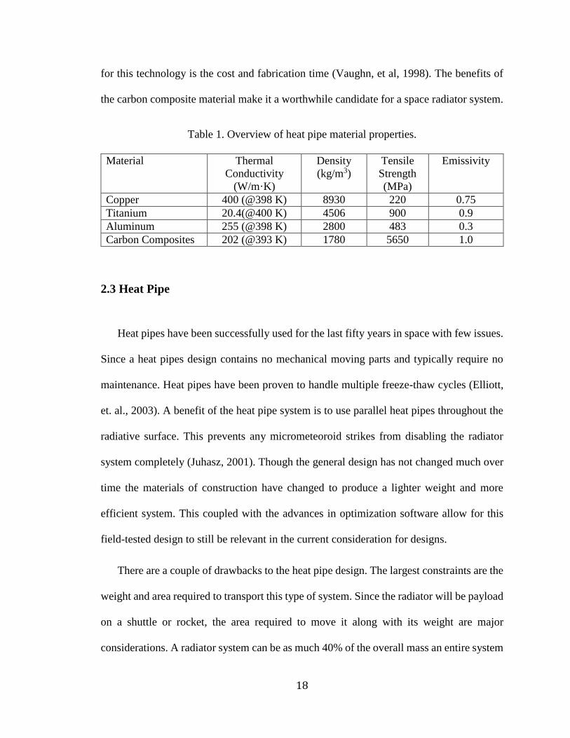
18
for this technology is the cost and fabrication time (Vaughn, et al, 1998). The benefits of
the carbon composite material make it a worthwhile candidate for a space radiator system.
Table 1. Overview of heat pipe material properties.
Material Thermal
Conductivity
(W/m·K)
Density
(kg/m3)
Tensile
Strength
(MPa)
Emissivity
Copper 400 (@398 K) 8930 220 0.75
Titanium 20.4(@400 K) 4506 900 0.9
Aluminum 255 (@398 K) 2800 483 0.3
Carbon Composites 202 (@393 K) 1780 5650 1.0
2.3 Heat Pipe
Heat pipes have been successfully used for the last fifty years in space with few issues.
Since a heat pipes design contains no mechanical moving parts and typically require no
maintenance. Heat pipes have been proven to handle multiple freeze-thaw cycles (Elliott,
et. al., 2003). A benefit of the heat pipe system is to use parallel heat pipes throughout the
radiative surface. This prevents any micrometeoroid strikes from disabling the radiator
system completely (Juhasz, 2001). Though the general design has not changed much over
time the materials of construction have changed to produce a lighter weight and more
efficient system. This coupled with the advances in optimization software allow for this
field-tested design to still be relevant in the current consideration for designs.
There are a couple of drawbacks to the heat pipe design. The largest constraints are the
weight and area required to transport this type of system. Since the radiator will be payload
on a shuttle or rocket, the area required to move it along with its weight are major
considerations. A radiator system can be as much 40% of the overall mass an entire system

19
(Tagliafico and Fossa, 1997). The other drawback is the efficiency of the heat pipe itself.
Lunar and space environments provide no means convective heat transfer. This means that
the heat pipe must be able to radiate enough heat to meet system requirements.
Heat pipes are a tried and true system for heat transfer in a purely radiative
environment. They have been successfully used numerous times in low and no gravity
environments. This type of design allows for a space radiator to be composed of a
multiplicity of independently operating segments, a random micrometeoroid puncture of
the radiator would result in the loss of only the punctured segment, not the entire radiator
(Juhasz, 2001). Combining this time tested design with modern materials of construction
and current design optimization techniques will provide a feasible radiator design that does
not require years of research and study to be operational. The heat pipe design utilizing a
lightweight ceramic woven fabric for structural strength along with a metallic liner for
working fluid retention can yield significant reductions in the mass of radiator systems
(Antoniak et al., 1991). Initially intended for high temperature systems, the technology can
be extended to cover a broad range of temperatures by properly selecting alternate heat
pipe working fluids and compatible liner material (Juhasz, 1998).
2.4 Fin and Fin Integrated with Heat Pipe
Fins are used in radiator systems to increase the surface area over which heat is
transferred. Through the use of fins the surface area is increased while adding a minimal
amount of weight to the system. This allows for the radiator system to be smaller and lighter
while having the same overall surface area of a larger system that has no fins. In space
applications, the fins allow for a larger surface to radiate heat into space. The heat radiated
by the fins is shown to be proportional to the cube of the heat pipe temperature, two-thirds

20
power of the emissivity, and one-third power of the thermal conductivity to density of fin
material (Naumann, 2004). Once the heat transfer is known the dimensions of the fins can
be calculated. The optimum dimension for the fins depends on the opening angle and the
emissivity and the profile not the specific values of fin heat dissipation or the fin volume
(Krikkis & Razelos, 2002). The effectiveness of the fins also needs to be calculated to
determine whether fins are necessary to the system. Effectiveness of the fin expressed
through apparent emittance, the ratio of actual total radiative heat loss to the ideal heat loss
by a black, isothermal fin (Krishnaprakas & Narayana). If the effectiveness is calculated to
be less than two the fins are not necessary to the system (Incropera and DeWitt, 1996).
There are two primary types of fins for radiator systems; solid fins and heat pipe fins.
Fins that attach directly to the heat source are considered solid fins. Heat pipe fins are part
of the heat pipe system and remove heat from the system to working fluid and radiate the
heat into space through the fins attached to heat pipes. These fins can either be flush
mounted or inserted into the heat pipe (Bowmann, Moss, et al., 1999). Then there is the
geometry of the fin. The fin shapes that are most common are rectangular, trapezoidal, and
triangular.
The purpose of adding fins to a system is to reduce weight while maintaining heat
transfer area. For this reason, heat pipe fins are beneficial when weight is a design
parameter (Bowmann, Storey, et al, 1999). Heat pipe fins typically weigh less than the
corresponding solid fins given by a required heat transfer area. This is due to the heat pipe
being hollow. Because of the proximity of the working fluid to the heat transfer area, heat
pipe fins are usually more efficient than solid fins for radiative environments (Bowmann
and Maynes, 2001).
21
Fin geometry is the other major area of concern in design. Rectangular fins provide the
greatest area for heat transfer. However, these fins also increase the weight of the radiator
significantly. Trapezoidal fins allow for a slight reduction in weight but without a
significant reduction heat transfer area. Triangular fins are half the weight of their
rectangular counterparts and transfer between five and fifteen percent less heat (Schnurr,
1975).
2.5 Radiator Fluid Selection
Almost any fluid can be used in a radiator system. The type of fluid is based on the
materials and temperatures of the system. The most common working fluids are water,
ammonia, and exotic materials such as liquid metals. Other materials are suitable on a case-
by-case basis.
Ammonia is the most common fluid used in extraterrestrial radiator applications. This
is due to its low freezing point and vapor temperature. For operating temperatures between
200 and 300 K ammonia is an ideal working fluid (Juhasz, 2007). Ammonia, in anhydrous
form, is compatible with many typical materials of construction including aluminum,
nickel, ceramic and stainless steel. It does corrode materials such as titanium and copper
and other materials of construction should be considered.
For slightly higher temperatures, purified water is an option. Water is useful when the
radiator operating temperature is between 300 and 500 K (Juhasz, 2007). This prevents the
water from freezing or remaining in a vapor state. However, if freezing is of concern during
times of shutdown, additives such as propylene glycol can be added to the water to lower

22
the freezing point. Purified water is also compatible with most common types of structural
materials use in radiator fabrication.
When dealing with extreme temperatures, such as those for nuclear power plants, the
radiator working fluid is typically a metal or material that similar characteristics of a metal.
These are typically used in temperatures of 700 K and greater (Keddy, 1994). For this
reason, liquid metals are necessary for the operation of the radiator system. Liquid metals
are extremely corrosive. The corrosion rate is sensitive to the operating temperature and
the temperature change in the system (Thompson, 1961). The specific working fluid will
dictate the materials compatibility with the radiator structural material. If the two are
incompatible a liner in the radiator can be used to prevent contact as is done in Jushaz’s
radiator design.
2.6 Wick Design
Radiator wicks are used to transport the condensed liquid from the cold region of the
heat pipe to the hot region in low and no gravity environments. There are various wick
designs and materials. Three primary designs are: slab wicks, arterial wicks, and groove
wicks. Each design provides benefits for various radiator systems. The other wick
consideration is the material of which the wick is made.
The most basic design is the slab wick. In this design most of heat pipe filled with highly
permeable screen or other material. The vapor then condenses on the wick down the pipe
to be transported back to the evaporator section. This design is simple and easily
constructed. The major drawback is that there is a significant increase in weight.

23
Arterial wicks utilize a mesh or screen that covers the inside of the heat pipe. As the
fluid condenses on the walls of the heat pipe, the wick moves the fluid back to the
evaporator section. This design is efficient in that as the heat transfer through condensation
is taking place the fluid is already in the wick ready to be transported. This allows for a
thin layer of wicking material. An arterial design works well with alkali metals as well as
most other general operating fluids. The only drawback is that it is difficult to keep the
wick primed when using water at higher temperatures.
Grooved wicks provide a simple design by simply machining grooves into the heat pipe
material. The fluid condenses in the groves where it is transported back to the evaporator
section through the channels. These types of wicks offer easily reproducible behavior while
not adding additional weight to the system. However, this wick design is only feasible for
piping materials that can reasonably be machined.
The most common wick material in space radiator systems with water as a cooling
fluid is copper. Copper can be used in systems operating at less than 425 K due to its low
melting point. For systems operating over 425 K titanium is often considered for the wick
material.
2.7 Radiator Design Optimization
The radiator design optimization uses three major factors in optimization: heat transfer
rate, surface area of the radiator, and mass of the radiator. Fin design is an additional
optimization constraint when it applies to the design. Optimization can be done several
ways. The two primary approaches are optimizing mathematical models or using computer
programs to optimize a specific design. Each method has its strengths and weaknesses.

24
Mathematical models use fundamental equations to optimize portions of the
radiator. The general goal of radiator optimization is minimize the radiator mass for a given
heat storage and dissipation (Roy and Avanic, 2006). Using equations a general solution
for optimum design can be achieved. The types of optimizations can be linear, optimizing
the ratio of fin mass to heat pipe mass (Naumann, 2004), or using special decomposition
techniques to determine the maximum heat transfer rate per unit mass (Arslanturk, 2006).
This type of optimization provides a general form of optimization that can be altered to
optimize similar designs. The major drawback to this form of optimization is that it is often
times limited to a specific design. This is due to assumptions and addition/removal of terms
from the overarching equations.
Computer simulation modeling also allows for optimization of radiator design.
Programs like FLUENT®, Thermal Desktop®, and Space Nuclear Auxiliary Power
Analysis System (SNAPS)® optimize a specific design that has been drawn. The different
programs have different approaches to obtaining an optimized design. SNAPS® uses a
flowsheet design often used in chemical processing. Flowsheet software is useful for
performing steady-state heat and mass balances, sizing equipment, and running cost
analysis. (Diwekar and Morel, 1993) FLUENT® is a useful commercial software tool in
the design of a single small scale system, such as a single heat pipe and fin assembly while
Thermal Desktop® is ideal for large scale design of an overall system and the surroundings
(Siamidis, 2006). These modeling programs can produce numerical results of theoretical
operating parameters. This allows the designer to overlay the different design parameters
to optimize the system around desired operating parameters. The downside to this is every

25
design done using a computer program needs to be modeled and optimized to determine
the optimum design.

26
Chapter 3
Theory and Numerical Methods
There are many aspects of design that are considered in heat pipe design. The governing
equations of continuity, momentum and energy prevail in the system. Heat transfer
equations are then used to determine the amount of energy that can be transferred to the
surroundings. Computational fluid dynamics (CFD) programs use the above equations
along with the proper boundary conditions and additional input parameters, based on the
needs of the individual design, to numerically model a system.
3.1 Governing Equations
The energy equation is of utmost importance in radiator system design. This equation
describes the energy transfer both inside the system and energy transmission to the
surroundings. This transfer for the fluid is described by Equation 1.
𝛿
𝛿𝑡(𝜌 ∙ 𝐸) + ∇(𝜈(𝜌 ∙ 𝐸 + 𝑝)) = ∇ ∙ (𝑘𝑒𝑓𝑓 ∙ ∇𝑇 − ∑ ℎ𝑗 ∙ 𝑗𝑗 + (𝜏�̿�𝑓𝑓 ∙�⃗�)𝑗 ) + 𝑆ℎ
(1)
The effective conductivity is given as keff (W/m∙K). This effective conductivity is the
combined ability for all materials of a specific region in the design to conduct heat. The
diffusion flux of each possible component is represented by 𝐽𝑗⃗⃗⃗(kJ/m2∙K). This flux accounts
for the rate at which an individual component diffuses. This flux term is a summation of
the sensible enthalpy, h, multiplied by the diffusion flux for every component being
considered. Energy is represented by E (kJ) in the above equation. However, the energy is
a function sensible enthalpy, pressure, density, and kinetic energy as shown in Equation 2.

27
𝐸 = ℎ −𝑝
𝜌+
𝜈2
2 (2)
The sensible enthalpy used in energy equation above for an incompressible fluid is
shown in Equation 3.
ℎ = ∑ 𝑌𝑗 ∙ ℎ𝑗 +𝑝
𝜌𝑗 (3)
For the portion of the heat pipe that is in vapor form, the energy is represented by an
ideal gas as represented in Equation 4.
ℎ = ∑ 𝑌𝑗 ∙ ℎ𝑗𝑗 (4)
The Yj term is the mass fraction the component that is in the gas form and the hj term
is the sensible energy for the component. Equation 5 shows how the sensible enthalpy for
each component is calculated where Tref is 298.15 K. The specific heat for a component is
defined as cp,j.
ℎ𝑗 = ∫ 𝑐𝑝,𝑗𝑇
𝑇𝑟𝑒𝑓∙ 𝑑𝑇 (5)
The momentum equation is used in heat pipe design to describe the fluid movement in
the heat pipe. Since the fluid in the heat pipe can be in one or two phases this equation it
must account for both the liquid and vapor phases of the working fluid. FLUENT® also
couples the momentum equation with the mass conservation equation. The conservation of

28
mass is calculated using Equation 6, which shows that mass is a function of density,
velocity, and pressure change with respect to time.
𝛿𝜌
𝛿𝑡+ ∇ ∙ (𝜌�⃗�) = 𝑆𝑚 (6)
The momentum equation is also a function of velocity, density, and pressure change.
This equation, Equation 7, also takes into account stress tensors as well as gravitational
and external body forces.
𝛿
𝛿𝑡(𝜌�⃗�) + ∇ ∙ (𝜌�⃗��⃗�) = −∇𝑝 + ∇ ∙ (𝜏̿) + 𝜌�⃗� + �⃗� (7)
3.2 Fundamentals of Radiation Heat Transfer and Heat Pipe Efficiency
There are three types of heat transfer that should be considered for radiator design.
These heat transfer models are convection, conduction, and radiation. All of these methods
depend primarily on temperature gradients to move the heat. The difference is a transfer
constant parameter unique to each equation.
Convection is a method of heat transfer by which heat is transferred due to bulk fluid
movement. All environments that include a fluid have convection as a major component of
heat transfer either to or from the surrounding fluid. Since fluid motion is a function of
temperature fluctuations, there are few places that convection does not occur. In Equation
8 it is shown that convection is a function of the heat transfer coefficient (hc), the surface
area of heat transfer (A), and the temperature difference.
𝑄 = ℎ𝑐𝐴𝑑𝑇 (8)

29
Conduction heat transfer considers the heat transfer through a solid or fluid due to
contact. Equation 9 shows that conduction is a function of the thermal conductivity of the
material (k), the surface area of heat transfer (A), and the temperature gradient. This form
of heat transfer is a primary concern when there are large distances, thicknesses, which are
under consideration or in the case of heat transfer though a substance is the primary
concern.
𝑄 = 𝑘𝐴𝑑𝑇
𝑑𝑥 (9)
The final form of heat transfer is radiation. For most situations radiation is negligible
as compared to convection or conduction transfer. However, for extraterrestrial
environments it is the primary form of heat transfer to or from a system. Due to the lack of
atmospheric ambient fluid movement convection heat transfer is not a feasible design
consideration. For this design the walls of the heat pipe are relatively thin and made of a
highly conductive material thus making conduction a negligible design consideration.
Since this system would operate on the lunar surface, radiation heat transfer is the primary
source of heat transfer.
The materials of construction can be classified as either blackbody or grey body. The
blackbody radiator, also called the ideal radiator, absorbs all the energy it encounters
reflecting nothing back into the surroundings. It provides a theoretical maximum value for
a design. Typically blackbody radiators are considered theoretical only due to the perfect
transmission of energy. The energy transfer in an ideal system is due only to the Stefan-
Boltzman constant, surface area, and operating temperature raised to the fourth power as
shown in Equation 10.
30
𝑄𝑖𝑑𝑒𝑎𝑙 = 𝜎𝐴𝑇4 (10)
The other type of radiator is a grey body radiator. This type of radiator both absorbs
and emits energy into the system. The equation for grey bodies is similar to that of
blackbodies. The grey body equation contains the effect of the material, emissivity, which
accounts for the imperfect radiation. The basic equation for radiation heat transfer is shown
in Equation 11 and adds the effect of emissivity and the sink or surrounding temperature
raised to the fourth power.
𝑄𝑟𝑒𝑎𝑙 = 𝜎𝜀𝐴𝑟𝑎𝑑(𝑇𝑖𝑛4 − 𝑇𝑠𝑖𝑛𝑘
4 ) (11)
This equation considers the emissivity, , the Stefan-Boltzman constant, , and the
temperature of the surface and surroundings. The emissivity of an object is the objects
ability to radiate heat from the surface. For an object that can radiate all the heat from its
surface the emissivity is one. This type of object is a black body and is generally considered
theoretical. Most substances cannot disperse all the heat they contain via radiation from
their surface. These are considered grey body radiators. They have an emissivity ranging
from zero to one. The emissivity for a substance is determined by empirical means and is
considered a property of that material. By including the emissivity the amount of heat
transferred from the surface is decreased from that if its black body counterpart; however,
this provides a more accurate depiction of the actual expected heat loss. The Stefan-
Boltzman constant is a proportionality constant that is based on the Stefan-Boltzmann Law.
This law is the governing law for black bodies that states the radiation heat emitted from a
substance’s surface is proportional to the absolute temperature to the fourth power.

31
To determine the efficiency of the heat pipe design the theoretical maximum is
compared to the actual value as given in Equation 12. For theoretical calculations this
would be the comparison of the black body radiation power to that of the grey body. For
the computer aided design the efficiency would be the comparison of the computer design
power to the theoretical grey body value. Hence, the following equation would hold.
𝜂 =𝑄𝑐𝑎𝑙𝑐𝑢𝑙𝑎𝑡𝑒𝑑
𝑄𝑡ℎ𝑒𝑜𝑟𝑒𝑡𝑖𝑐𝑎𝑙 (12)
In an ideal situation the power calculated would be nearly the power that theoretically
would be dispersed.
3.3 Models Used in FLUENT
FLUENT® is a commercial CFD software which can be readily used in radiation heat
transfer modeling. The program uses various numerical methods to determine temperature
and power results. There are five numerical solving techniques that are included in
FLUENT®. These solvers are discrete transfer radiation model (DTRM), P-1 radiation
model. Rosseland radiation model, surface-to-surface (S2S) radiation model, and discrete
ordinates (DO) model. Each method of solving has its valid uses and limitations. These
are briefly described below.
Advantages and Limitations of the DTRM
DTRM is a relatively simple model that applies to a wide range of optical thicknesses.
Increasing the number of rays in the calculation can increase this models accuracy.
However, there are certain limitations for this model. The model assumes that all surfaces
are diffuse and exhibit grey body radiation. The effect of scattering is not considered in the

32
DTRM model. It is not able to handle parallel processing or sliding meshes and can be time
consuming for a large number of rays.
Advantages and Limitations of the P-1 Model
The P-1 model uses the radiative transfer equation (RTE) to make the design easy to
solve. The RTE states the a beam of light loses energy through the divergence, absorption,
and scattering and gains energy from light sources in the medium and scattering of other
beams towards the beam of light. This model also takes into account the effect of scattering.
For optically large thicknesses and complex geometries the model is also acceptable. There
are certain limitations for this model. The model assumes that all surfaces are diffuse and
exhibit grey body radiation. When used to solve more complex geometries accuracy is lost.
It is not able to handle parallel processing or sliding meshes and can be time consuming
for a large number of rays. The P-1 model may over-predict radiative fluxes when localized
heat sources or sinks are present.
Advantages and Limitations of the Rosseland Model
The Rosseland model does not solve for incident radiation like the P-1 model. In not
doing this step the model has a faster computational time and does not require the same
amount of memory. However, there are a couple of limitations for this model. The
Rosseland model can only be used for extremely optically thick materials. Also, it cannot
be used in conjunction with a density based solver thus requires the pressure based solver
to be enabled.
Advantages and Limitations of the S2S Model

33
The surface-to-surface (S2S) radiation model used in modeling enclosed radiative
transfer systems. The S2S model has a faster solving time than other models though
depending on geometry. This is particularly true for polyhedral cells. This model is often
used when modeling systems for extraterrestrial heat rejection systems.
The limitations of the surface-to-surface model are that it assumes all surfaces grey
surfaces that are diffuse. This model cannot be used for participating radiation designs,
non-conformal interfaces, or symmetry or periodic boundary conditions. Also of note is
that memory requirements increase rapidly if view factors are not clustered.
Advantages and Limitations of the DO Model
The discrete ordinates model has benefits in that it can be used over a vast range of
optical thicknesses. It can be used to solve problems that are encompassed in other models.
This model can also be used to evaluate semi-transparent walls. The time and memory for
calculations is modest compared to other models.

34
Chapter 4
Benchmark and Validation Studies
An independent mesh study was conducted on a basic design of a heat pipe with
integrated fin. This was done to ensure that the resulting values of the program were
independent of the mesh size. In doing a mesh independent study, the results of the model
represent a true and accurate value. Once the minimum mesh size required for the design
was determined the wick study and benchmark could be calculated.
Next a wick study was conducted. For this design the wick was not modeled. Since the
wick is used to transport the fluid in the heat pipe the wick effect had to be considered. To
determine a numerical representation of the equivalent wick performance, two papers
Woloshun, et al. (1993) and Dickenson (1996) that evaluated the temperature profile of the
wick were evaluated. The results of this were used to simulate the effect of the wick in the
design.
Benchmarking is done to ensure that the user and the program are producing valid
results. For this purpose two separate designs were used as benchmarks. One benchmark
was to validate FLUENT® and the other to validate user results. The benchmark design is
that of a heat pipe design that closely relates to the design being considered. This
benchmark allows for the comparison between computer design and laboratory and actual
working data. This can show any biases in the design and potential problems in the set-up
conditions.
4.1 Validation Study
4.1.1 Purpose

35
The mesh independent study is used to determine the point in meshing a design that the
results vary only slightly with a change in the mesh. This value can then be used to assure
that the number of nodes or cells used exceed this minimum value. If the minimum value
is exceeded, the results are no longer dependent on the size of the mesh. Performing a mesh
independent study assures that the design is only changing with boundary conditions and
not with mesh conditions.
4.1.2 Methodology
The most general design of a heat pipe with integrated fin was selected for this study
as shown in Figure 5. This design consisted of a heat pipe with integrated fin. The heat
pipe had an outer diameter of 25 mm and an inner pipe diameter of 23 mm. The design had
a fin length of 25 mm and had a thickness of 2 mm. The heat pipe and fins were 300 mm.
The end caps were also 2 mm thick. This selection was due to the fact that this design was
the starting point for all other models. The mesh size was varied from 4738 cells to 19609
elements. The temperature along the pipe at various intervals was analyzed as a function
of the number of cells. This was then evaluated to determine the minimum number of cells
necessary for the mesh to no longer affect the temperature results.

36
Heat Pipe Diameter – 25 mm
Heat Pipe and Fin Length – 300 mm
Fin Length – 25 mm
Insertion Tube Diameter – 23 mm
Insertion Tube Length - 76 mm
Figure 5. Three-dimensional design for validation study.
Four mesh discretizations were analyzed. The analysis included 4738, 9486, 11461,
and 19609 number of elements. The first represented a coarse mesh while the final
represented a fine mesh with high smoothing. The values in between are values that were
easily represented to analyze the transition section to determine the minimum mesh size
for independence.
4.1.3 Results
The validation study was carried out on the heat pipe with integrated fin. This showed
that the temperature gradient was somewhat dependent on the mesh when the number of
cells was less than 11461. However once the number of elements exceeded 11461 the
temperature became stable. The following, Figure 6, shows the graphical representation of
the above results of temperatures every 75 mm along the outside of the heat pipe.

37
Figure 6. Results of independent mesh study.
As this is a simple geometry, the relatively small number of cells necessary for the
temperature to become independent of the mesh is expected. By using a mesh in the 12000
range the mesh independence of the various geometries and fin comparison can be
expected.
4.2 Wick Performance Simulation
In order to accurately describe the performance of the heat pipe the performance of the
wick characteristics had to be determined since the wick structure was not to be modeled
in this design. Several papers, Woloshun, et al. (1993) and Dickenson (1996) describing
the performance of the wick were studied. From the results of these papers a profile was
created.
580
600
620
640
660
680
700
0 100 200 300
Tem
pe
ratu
re (
K)
Axial Length (mm)
Mesh Independent Study
Coarse Mesh (4738elements)
Medium Mesh (9486elements)
Medium Mesh (11461elements)
Fine Mesh (19609elements)

38
The papers of Woloshun, et al. (1993) and Dickenson (1996) were evaluated to
determine the behavior of heat pipe slab wick. These papers showed similar profiles
regardless of the operating temperatures or the ambient temperatures. Since there seemed
to be no dependency on these conditions it was assumed that this general profile was
standard among all heat pipes in low and no gravity environments. The thermocouple
results of these papers were taken and entered into Excel to generate two graphs. From this
graph a linear regression was done using Excel, and a third degree polynomial equation,
Equation 11, was generated. In this equation temperature, T, is given as a function of axial
length, x.
𝑇 = −1.4𝑥3 + 1.4893𝑥2 − 0.6724𝑥 + 0.9139 (13)
Though there were actually two equations generated, the equation with the lower
variance was selected to model the pipe interior. This equation was then used to create a
user-defined function (UDF) profile in FLUENT® to account for the equivalent wick
performance in the heat pipe. This technique is adequate for this design in that the interior
geometry is unchanged among all the heat pipe designs. However, this equation only
represents a slab wick design and cannot be used to represent any other wick
configurations.
4.3 Benchmark Study
4.3.1 Heat Pipe Design
This goal of this research was to investigate and compare the operation of a
microgravity, liquid-metal heat pipe in both laboratory and operational settings. There was
a project supported by the United States Air Force Institute of Technology as part of a

39
Master’s Thesis. (Dickenson, 1996) Heat pipe start-up from a frozen state, start-up from a
pre-heated state, steady state operations, as well as various wick designs for the afore
mentioned were considered. The research conducted on the heat pipe containing the
annular wick was of interest as it closely mimicked the Juhasz’s design to be modeled.
4.3.2 Dimensions of Heat Pipe
The design of the heat pipe tested by Dickenson (1996) also closely resembled that of
the Juhasz’s design. The heat pipe tested was 610 mm in length, with 521 mm being the
condenser and 89 mm being the evaporator. The heat pipe outer diameter was 23 mm in
diameter and had a wall thickness of 0.89 mm. Stainless steel 304 was used to make the
heat pipe and the wick material. The working fluid to convey the heat transfer was
potassium.
4.3.3 Boundary Conditions and Operating Parameters
This design had several operating temperatures. For the sake of comparison the 700 K
operating temperature was the trial that was used for comparison. The laboratory tests were
carried out in what is characterized as “room temperature” without a value provided. The
shuttle flight test data had rejection temperatures ranging between 10°C and 35°C. The
wick boundary condition was set using the wick study values to approximate the
performance of the wick.
In this trail the parameters for the materials were provided. A thermal conductivity of
21.2 W/m·K was given for the 304 stainless steel pipe material while the wick material had
a thermal conductivity of 29.11 W/m·K. The heat capacity for 304 stainless steel was 569.5
J/kg·K. Finally, the density for the stainless steel was given to be 7900 kg/m3.

40
4.3.4 Numerical Modeling of Heat Pipe Design
A numerical modeling of heat pipe design using FLUENT® was created using the given
parameters for the laboratory and shuttle data. The design included a 610 mm long heat
pipe with an integrated fin. The condenser section of heat pipe was 521 mm in length with
an outer diameter of 23 mm. The evaporator section was 89 mm in length and had an outer
diameter of 22 mm. The schematic of this is shown in Figure 7. The heat pipe had a wall
thickness of 2 mm. Stainless steel 304 was used to in the modeling of the heat pipe. The
working fluid to convey the heat transfer in the model was potassium.
Heat Pipe Diameter – 23 mm
Heat Pipe Length – 521 mm
Insertion Tube Diameter – 22 mm
Insertion Tube Length - 89 mm
Figure 7. Schematic of heat pipe with integrated fin from numerical modeling design for
benchmark study.
4.3.5 Comparison of Numerical Results
This numerical data obtained from FLUENT® was compared to the results provided by
Dickenson (1996). The numerical results provided the same temperature profile as the
laboratory and flight tests data gave as shown in Figure 8. Both the numerical results

41
obtained from FLUENT® and the flight test data begin at 600 K, drop to the 480 K range
along the condenser section, and drop quickly at the end cap to about 300 K. The numerical
values obtained from FLUENT® were slightly higher than that of the benchmark study as
shown in Table 2. However, the values were close enough to believe that FLUENT has
accurately provided the satisfied numerical results compared to modeled results obtained
from the laboratory data.
Figure 8. Axial length versus surface temperature comparison for benchmark and
numerical results.
0
100
200
300
400
500
600
700
0 200 400 600 800
Tem
pe
ratu
re (
K)
Axial Length (mm)
Benchmark Comparison
Benchmark Data
Modeled Results

42
Table 2. Benchmark and FLUENT data comparison
Axial
Length Benchmark FLUENT
Results
Modeled
Results
Percentage
Difference
mm K K %
0 600 595 0.83
50 565 548 3.01
100 470 469 0.21
150 465 468 0.64
200 470 468 0.43
250 455 468 2.78
300 470 469 0.21
350 460 469 1.92
400 470 468 0.43
450 470 468 0.43
500 455 468 2.78
550 400 386 3.50
600 313 305 2.56
The numerical modeling of heat pipe design provides a smoother temperature profile
in the condenser section of the heat pipe. It does not exactly mimic the behavior of the test
data in the first and last 100 mm of the pipe. The difference in the FLUENT and benchmark
data is a result of smoothing within FLUENT; however the differences in temperature are
less than 3.5%. Because FLUENT shows a greater decrease in the temperature of the heat
pipe in the first and last 100 mm, the computer model is likely under reporting the power
output of the heat pipe.

43
Chapter 5
Results and Discussions
Due to the size constraints of a shuttle load the radiator would need to be designed in
segments. The reason for this is twofold. This design will make for easier transport than
one large system and in minimizes the risk of complete failure if the operational radiator is
damaged. For this design an individual heat pipe is to be modeled using FLUENT®.
The individual heat pipe design is based on that of Albert Juhasz (1998). In his
publication “Design Considerations for Lightweight Space Radiators” he provides a design
consisting of a heat pipe 25 mm in diameter, 300 mm in length, with a 1 mm thick wall.
The design also specifies fin dimensions of 25 mm in width and 1 mm thickness running
the entire length of the heat pipe.
Every design contained an insertion portion that would be used as the evaporator
section. This portion would be inserted in a main pipe that carried a high temperature fluid.
The length of the evaporator section was 76 mm and had an outer diameter of 24 mm. This
section also had a wall thickness of 2 mm due to constraints of the program and the mesh.
The specifications for this design are shown in Figure 9.

44
Figure 9. Heat pipe design. (Juhasz, 1998)
The initial goal was to determine that the heat pipe design was the best design for this
radiator design. This was done by comparing various geometries. Rectangular solid,
cylindrical solid, cylindrical solid with fins, heat pipe without fins, and the above design
were modeled and the results compared. All the designs maintained the same radiation
surface area and had the same parameters used for evaluation.
Once the heat pipe design was proven to be a feasible design, the fin length needed to
be evaluated to determine the best length in order to minimize the size while maximizing
the heat transfer. This was accomplished through varying the ratio of fin width to fin length.
The ratio of fin length to width was evaluated at 0 (from the above design), 0.25, 0.5, 0.75,
1 (from the above design), 1.25, and 1.5.
The temperature profiles and power output of the designs outlined above were modeled
using FLUENT®. The designs were created in FLUENT® and modeled using the P-1
radiation model. The P-1 model was used due to a relatively simple geometry but the need
to account for scattering. Results obtained from FLUENT® are shown as positive, for
incoming power values, or negative for power that is leaving the system. As is mentioned
45
in Chapter 3, the P-1 model tends to over predict the radiative fluxes. In those cases the
net flux is given as a negative value. Due to this possibility of over prediction, a relative
error was calculated for each design. This error calculation is used as a design control to
maintain the discrepancies in the results to less than 5%. Along with the radiation area and
volume of the various designs were determined using FLUENT® analysis. These values
along with power and temperature data were used to compare geometrical shapes, pipe
width to length ratios, and profile data.
5.1 General Methodology
The basic steps were used in each design. To begin FLUENT® was chosen in the
ANSYS Workbench to create a new project. Then the geometry was created using the
geometry module. The geometry varied based on the individual case and these designs are
discussed in their relative sections. Once the geometry was created and saved, the mesh
module was selected. In these section individual components of the design such as the
insertion tube, fins, end cap, and pipe interior were named in order to be able to set
individual boundary conditions or look at individual performance once the simulation was
completed. After all the components were named, the mesh was generated and the file
saved.
FLUENT® was selected from the workbench screen. Once the meshed model opened,
the energy equation was enabled and radiation model was selected. A screen appeared to
allow for the selection of a specific radiation model. From this screen, the P-1 model was
selected. The scattering is assumed isotropic and the scattering coefficient remained zero.
Materials properties were created for the carbon composite material. The fluid was set as
potassium using the parameters form the benchmark study. Boundary conditions were set

46
for each of the defined areas of the geometry. The boundary conditions were standard for
each design. The solid designs did not contain a pipe interior and the designs without fins
did not have conditions set for them. The insertion tube was set at a constant temperature
of 700 K. The outer wall and fins boundary condition was defined by the radiation
parameters of emissivity of 0.8 and external temperature of 230 K. The pipe interior, as
discussed above, was defined using a user-defined function to approximate the equivalent
wick performance.
5.2 Parametric Comparison
The first objective was to consider various geometries for a heat pipe design. The
geometries include a rectangular solid, a cylindrical solid, a cylindrical solid with fins, a
heat pipe, and a heat pipe with 25 mm fins. This was done to ensure that a heat pipe was a
feasible design choice in both power output and power per unit mass.
5.2.1 Rectangular Solid
The rectangular solid consisted of a base rectangle of 22 mm by 22 mm. This was
extruded to a length of 600 mm. The schematic of this design is shown in Figure 10. This
geometry had a power input of 153.59 W and an output of 157.00 W. The raw data from
FLUENT® is shown in Table 3. This power output translated to a power per radiation area
of 2963.94 W/m2 and a power per mass of 165.68 W/kg. As compared to the theoretical
value for the radiation area the efficiency of the rectangular design is 27.5%.

47
Square Top – 22 mm
Length – 600 mm
Insertion Tube – 21 mm
Insertion Tube Length - 76 mm
Figure 10. Schematic of rectangular solid.
Table 3. Power values for rectangular solid.
Rectangular Solid Power (W)
Insertion Tube 153.59276
Outer Radiation Surface -157.00218
Net -3.4094201
Error 2.171575006 %
The temperature profile of the rectangular solid is shown in Figure 11. The profile
is what would be expected of a solid material. Since the only means of heat transport
through the solid is conduction, the temperature is much higher near the insertion tube
and drops along the axis. The insertion tube temperature is held at 700 K and the end
temperature is 410 K. The temperature drops 200 K in the first half of the rectangular
solid. This can be compared to the 90 K drop along the second half.

48
Figure 11. Temperature (K) profile of rectangular solid.
5.2.2 Cylindrical Solid
The cylindrical solid consisted of a base circle with a diameter of 25 mm. This was
extruded to a length of 675 mm. Figure 12 shows the solid cylinder with the dimensions.
Cylindrical solid geometry had a power input of 141.89 W and an output of 149.21 W. The
numerical values obtained from FLUENT® are provided in Table 4. This translated to a
power per radiation area of 2738.80 W/m2 and a power per mass of 157.46 W/kg. As
compared to the theoretical value for the radiation area the efficiency of the rectangular
design is 25.4 %.
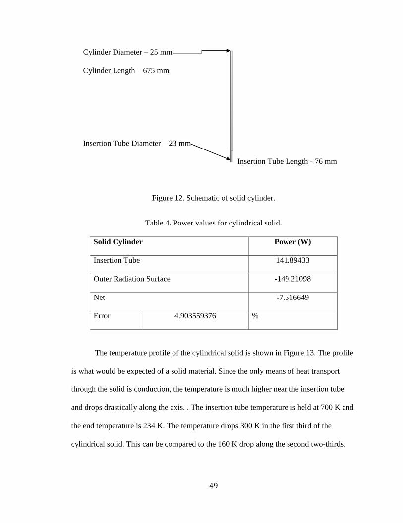
49
Cylinder Diameter – 25 mm
Cylinder Length – 675 mm
Insertion Tube Diameter – 23 mm
Insertion Tube Length - 76 mm
Figure 12. Schematic of solid cylinder.
Table 4. Power values for cylindrical solid.
Solid Cylinder Power (W)
Insertion Tube 141.89433
Outer Radiation Surface -149.21098
Net -7.316649
Error 4.903559376 %
The temperature profile of the cylindrical solid is shown in Figure 13. The profile
is what would be expected of a solid material. Since the only means of heat transport
through the solid is conduction, the temperature is much higher near the insertion tube
and drops drastically along the axis. . The insertion tube temperature is held at 700 K and
the end temperature is 234 K. The temperature drops 300 K in the first third of the
cylindrical solid. This can be compared to the 160 K drop along the second two-thirds.

50
Figure 13. Temperature (K) profile of cylindrical solid.
5.2.3 Cylindrical Solid with Fins
The cylindrical solid consisted of a base circle with a diameter of 25 mm. This was
integrated with the fins so as to produce the design proposed by Juhasz (1998). The fins
were 25 mm in length but 2 mm in width due to limitations of the program and mesh. This
was extruded to a length of 300 mm. A schematic drawing of this is shown in Figure 14.
The cylindrical solid with fin geometry had a power input of 220.61 W and an output of
225.35 W. The numerical values obtained from FLUENT® are provided in Table 5. This
translated to a power per radiation area of 4194.12 W/m2 and a power per mass of 384.36
W/kg. As compared to the theoretical value for the radiation area the efficiency of the
rectangular design is 38.9%.

51
Cylinder Diameter – 25 mm
Cylinder and Fin Length – 300 mm
Fin Length – 25 mm
Insertion Tube Diameter – 23 mm
Insertion Tube Length - 76 mm
Figure 14. Schematic of cylindrical solid with fins.
Table 5. Power values for solid cylinder with fins.
Solid Cylinder with Fins Power (W)
Fins -127.2424
Insertion Tube 220.60663
Outer Radiation Surface of Pipe -98.106845
Net -4.7426183
Error 2.104563652 %
The temperature profile of the cylindrical solid with fins is shown in Figure 15. The
profile is what would be expected of a solid material that has fins. Since the only means
of heat transport through the solid is conduction, the temperature is much higher near the
insertion tube. However, unlike the solid cylinder, the fins increase the surface area of
radiation allowed the heat to dissipate up the solid and creates a much broader gradient.
The insertion tube temperature is held at 700 K and the end temperature is 486 K. The

52
temperature drops 160 K in the first half of the cylindrical solid. The rest of the
temperature drop, 64 K, occurs over the rest of the length.
Figure 15. Temperature (K) profile of solid cylinder with fins.
5.2.4 Heat Pipe
The heat pipe outer cylinder consisted of a base circle with a diameter of 25 mm. An
inner circle of 23 mm was created to make a hollow heat pipe. The wall of the heat pipe
was 2 mm in width due to limitations of the program and mesh. Then end caps of 23 mm
in diameter and 2 mm in thickness were created and the material merged into the existing
heat pipe material. This was extruded to a length of 675 mm. This schematic is shown in
Figure 16. The heat pipe geometry had a power input of 110.3788 W and an output of

53
110.3786 W. The numerical values obtained from FLUENT® are given in Table 6. This
translated to a power per radiation area of 2053.96 W/m2 and a power per mass of 116.48
W/kg. As compared to the theoretical value for the radiation area the efficiency of the
rectangular design is 19.08%.
Heat Pipe Diameter – 25 mm
Heat Pipe Length – 300 mm
Insertion Tube Diameter – 23 mm
Insertion Tube Length - 76 mm
Figure 16. Schematic of heat pipe with no fin.
Table 6. Power values for heat pipe with no fin.
Heat Pipe Power (W)
With Profile
End Cap 0.85611307
Insertion tube 4.1803685
Pipe interior 105.3424
Outer Radiation Surface of Pipe -110.37865
Net 0.000234192
Error 0.000212171 %

54
The temperature profile of the heat pipe is shown in Figure 17. The profile is what
would be expected of a hollow material utilizing convective heat transfer inside. By using
potassium to transport the heat from the insertion tube to the end cap, the temperature
decrease along the heat pipe is drastically reduced. The high temperature along the length
of the heat pipe assures a high heat flux from the heat pipe. The insertion tube
temperature is held at 700 K and the end temperature is 617 K. The temperature drops
160 K in the first third of the heat pipe. This can be compared to the 23 K drop along the
second two-thirds.
Figure 17. Temperature (K) contour of heat pipe with no fin.
5.2.5 Heat Pipe with Fins

55
The outer cylinder consisted of a base circle with a diameter of 25 mm. An inner circle
of 23 mm was created to make a hollow heat pipe. Then end caps of 23 mm in diameter
and 2 mm in thickness were created and the material merged into the existing heat pipe
material. This was integrated with the fins so as to produce the design proposed by Juhasz
(1998). The fins were 25 mm in width but 2 mm in thickness due to limitations of the
program and mesh. This was extruded to a length of 300 mm. The schematic of this design
is shown in Figure 18.
Heat Pipe Diameter – 25 mm
Heat Pipe and Fin Length – 300 mm
Fin Length – 25 mm
Insertion Tube Diameter – 23 mm
Insertion Tube Length - 76 mm
Figure 18. Schematic of heat pipe with integrated fin.
The heat pipe geometry with fin length to diameter ratio of 1.0 had a power input of
430.72 W and an output of 441.76 W. The numerical values obtained from FLUENT® are
provided in Table 7. This translated to a power per radiation area of 8081.96 W/m2 and a
power per mass of 1906.60 W/kg. As compared to the theoretical value for the radiation
area the efficiency of the rectangular design is 75.08%.

56
Table 7. Power values for heat pipe with fin.
Heat Pipe 1.0 Ratio Power (W)
With Profile
End Cap -150.38675
Fin -162.12975
Insertion tube 151.37973
Pipe interior 279.33459
Outer Radiation Surface of Pipe -129.24197
Net -11.04415
Error 2.500042614 %
The temperature profile of the heat pipe is shown in Figure 19. The insertion tube
temperature is held at 700 K and the end temperature is 425 K. The temperature drops only
200 K along the majority of the heat pipe. The profile is what would be expected of a
hollow material utilizing convective heat transfer inside. By using potassium to transport
the heat from the insertion tube to the end cap, the temperature decreases along the heat
pipe is drastically reduced. The high temperature along the length of the heat pipe assures
a high heat flux from the heat pipe

57
Figure 19. Temperature (K) contour of heat pipe with 1.0 fin width to pipe length ratio.
5.2.6 Results and Discussions of Parametric Comparison
The following images are the temperature contours, shown in Figure 20, of the
simulation. It can be noted that by introspection that the heat pipe with fins geometry out
performs the other geometries. This geometry provides the highest temperature difference
along the length. This in turn provides the greatest ability for heat removal.

58
(a) (b) (c) (d)
Figure 20. Temperature (K) comparison of various geometries. (a) Cylindrical Solid (b)
Cylindrical Solid with fins (c) Heat Pipe and (d) Heat Pipe with fins.
By comparing the results of the various geometries with similar radiation areas we can
ascertain the best design for a radiator system. This is achieved by comparing the power
output per unit mass and the power output per unit radiation area. The design chosen was
a balance between the maximum amount of power per unit mass and maximum power per
unit area. This should optimize the power output while reducing the weight of a system. In
Table 8 the values of the various geometries considered are listed along with the power per
unit area, power per unit mass, theoretical output, and efficiency. Figure 21 shows a bar
graph of the power per unit area for the different geometries. From this figure it is clear to
find that the heat pipe with fins is the best performer. In Figure 22, which compares the
power per unit mass, the heat pipe with fins also far exceeds the other designs. These results
are expected as the heat pipe allows the greatest radiation area but also allows for better

59
heat transfer along the heat pipe due to the working fluid being able to move along the
interior of the pipe, thus keeping the temperature along the pipe higher.
Table 8. Comparison of power per unit area, power per unit mass, and efficiency of
various geometries.
Geometry Output Area Mass Power/Area Power/Mass
Theoretical
Power
Output Efficiency
W m2 kg W/m2 W/kg W %
Rectangular
Solid 157.00 0.05 0.95 3140.00 165.68 538.23 29.17
Cylindrical
Solid 149.21 0.05 0.95 2984.20 157.46 538.23 27.72
Cylindrical
Solid with
Fins
225.35 0.05 0.59 4507.00 384.36 538.23 41.87
Heat Pipe 373.29 0.05 0.29 7465.80 1284.99 538.23 69.36
Heat Pipe
with Fins 441.76 0.05 0.23 8835.20 1906.60 538.23 82.08
Figure 21. Comparison of power per unit area for various geometries.
0.00
1000.00
2000.00
3000.00
4000.00
5000.00
6000.00
7000.00
8000.00
9000.00
1
Power/Area v Geometry Comparison
Rectangular Solid
Cylindrical Solid
Cylindrical Solid with Fins
Heat Pipe
Heat Pipe with Fins
Power/Area (W/m^2)
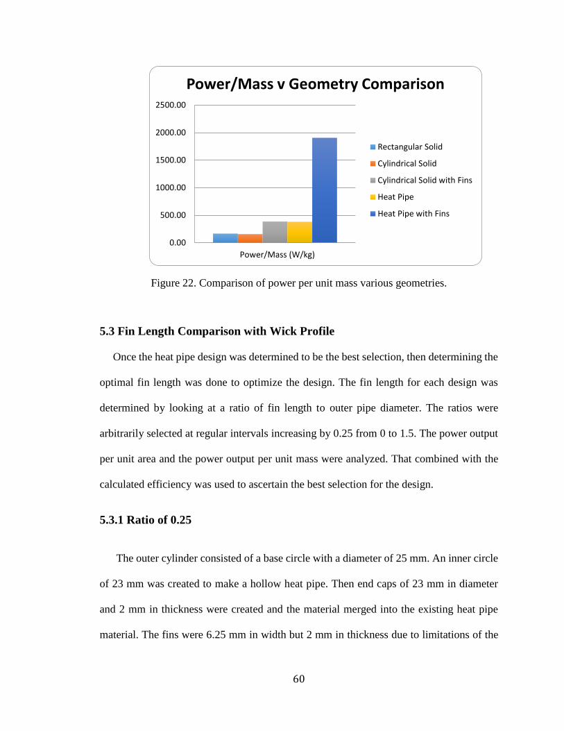
60
Figure 22. Comparison of power per unit mass various geometries.
5.3 Fin Length Comparison with Wick Profile
Once the heat pipe design was determined to be the best selection, then determining the
optimal fin length was done to optimize the design. The fin length for each design was
determined by looking at a ratio of fin length to outer pipe diameter. The ratios were
arbitrarily selected at regular intervals increasing by 0.25 from 0 to 1.5. The power output
per unit area and the power output per unit mass were analyzed. That combined with the
calculated efficiency was used to ascertain the best selection for the design.
5.3.1 Ratio of 0.25
The outer cylinder consisted of a base circle with a diameter of 25 mm. An inner circle
of 23 mm was created to make a hollow heat pipe. Then end caps of 23 mm in diameter
and 2 mm in thickness were created and the material merged into the existing heat pipe
material. The fins were 6.25 mm in width but 2 mm in thickness due to limitations of the
0.00
500.00
1000.00
1500.00
2000.00
2500.00
�Power/Mass (W/kg)
Power/Mass v Geometry Comparison
Rectangular Solid
Cylindrical Solid
Cylindrical Solid with Fins
Heat Pipe
Heat Pipe with Fins

61
program and mesh. This was extruded to a length of 300 mm. The schematic of this design
is shown in Figure 23.
Heat Pipe Diameter – 25 mm
Heat Pipe and Fin Length – 300 mm
Fin Length – 6.25 mm
Insertion Tube Diameter – 23 mm
Insertion Tube Length - 76 mm
Figure 23. Schematic of heat pipe with integrated fin using a fin ratio of 0.25.
The heat pipe geometry with fin length to heat pipe diameter ratio of 0.25 had a power
input of 336.36 W and an output of 339.36 W. This translated to a power per radiation
area of 10608.32 W/m2 and a power per mass of 1991.55 W/kg. The numerical data is
provided in Table 9. As compared to the theoretical value for the radiation area the
efficiency of the rectangular design is 98.5 %.
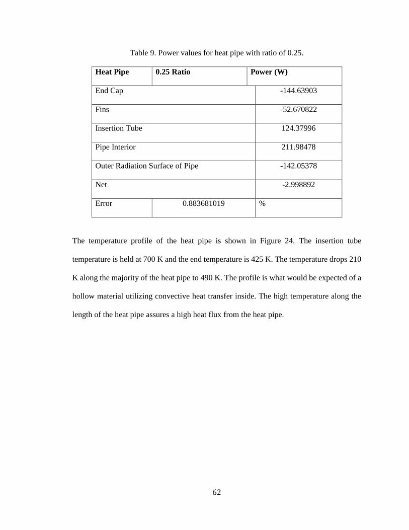
62
Table 9. Power values for heat pipe with ratio of 0.25.
Heat Pipe 0.25 Ratio Power (W)
End Cap -144.63903
Fins -52.670822
Insertion Tube 124.37996
Pipe Interior 211.98478
Outer Radiation Surface of Pipe -142.05378
Net -2.998892
Error 0.883681019 %
The temperature profile of the heat pipe is shown in Figure 24. The insertion tube
temperature is held at 700 K and the end temperature is 425 K. The temperature drops 210
K along the majority of the heat pipe to 490 K. The profile is what would be expected of a
hollow material utilizing convective heat transfer inside. The high temperature along the
length of the heat pipe assures a high heat flux from the heat pipe.

63
Figure 24. Temperature (K) contour of heat pipe with 0.25 fin width to pipe length ratio.
5.3.2 Ratio of 0.5
The outer cylinder consisted of a base circle with a diameter of 25 mm. An inner circle
of 23 mm was created to make a hollow heat pipe. Then end caps of 23 mm in diameter
and 2 mm in thickness were created and the material merged into the existing heat pipe
material. The fins were 12.5 mm in width but 2 mm in thickness due to limitations of the
program and mesh. This was extruded to a length of 300 mm. The schematic of this design
is shown in Figure 25.

64
Heat Pipe Diameter – 25 mm
Heat Pipe and Fin Length – 300 mm
Fin Length – 12.5 mm
Insertion Tube Diameter – 23 mm Insertion Tube Length - 76
mm
Figure 25. Schematic of heat pipe with integrated fin using a fin ratio of 0.5.
The heat pipe geometry with fin length to diameter ratio of 0.50 had a power input of
380.75 W and an output of 382.13 W. This translated to a power per radiation area of
9659.50 W/m2 and a power per mass of 2028.29 W/kg. As compared to the theoretical
value for the radiation area the efficiency of the rectangular design is 89.7%. The numerical
data is provided in Table 10.

65
Table 10. Power values for heat pipe with ratio of 0.5.
Heat Pipe 0.5 Ratio Power (W)
End Cap -155.52128
Fins -92.230587
Insertion Tube 134.75903
Pipe Interior 245.98682
Outer Radiation Surface of Pipe -134.3784
Net -1.384417
Error 0.362289282 %
The temperature profile of the heat pipe is shown in Figure 26. The insertion tube
temperature is held at 700 K and the end temperature is 425 K. The temperature drops only
214 K along the majority of the heat pipe. The temperature gradient is slightly less than the
0.25 ratio gradient varying by only 4 K.

66
Figure 26. Temperature (K) contour of heat pipe with 0.5 fin width to pipe length ratio.
5.3.3 Ratio of 0.75
The outer cylinder consisted of a base circle with a diameter of 25 mm. An inner circle
of 23 mm was created to make a hollow heat pipe. Then end caps of 23 mm in diameter
and 2 mm in thickness were created and the material merged into the existing heat pipe
material. The fins were 18.75 mm in width but 2 mm in thickness due to limitations of the
program and mesh. This was extruded to a length of 300 mm. The schematic of this design
is shown in Figure 27.

67
Heat Pipe Diameter – 25 mm
Heat Pipe and Fin Length – 300 mm
Fin Length – 18.75 mm
Insertion Tube Diameter – 23 mm Insertion Tube Length - 76 mm
Figure 27. Schematic of heat pipe with integrated fin using a fin ratio of 0.75.
The heat pipe geometry with fin length to diameter ratio of 0.75 had a power input of
404.86 W and an output of 406.96 W. This translated to a power per radiation area of
8693.87 W/m2 and a power per mass of 1949.04 W/kg. The numerical data is provided in
Table 11. As compared to the theoretical value for the radiation area the efficiency of the
rectangular design is 80.8%.

68
Table 11. Power values for heat pipe with ratio of 0.75.
Heat Pipe 0.75 Ratio Power (W)
With Profile
End Cap -147.84795
Fins -125.36772
Insertion Tube 143.03131
Pipe Interior 261.83097
Outer Radiation Surface of Pipe -133.74557
Net -2.0989544
Error 0.51576273 %
The temperature profile of the heat pipe is shown in Figure 28. The insertion tube
temperature is held at 700 K and the end temperature is 415 K. The temperature drops only
206 K along the majority of the heat pipe. The end cap temperature is less than that of the
0.25 or 0.5 ratio designs which is to be expected due to the increase in fin size.

69
Figure 28. Temperature (K) contour of heat pipe with 0.75 fin width to pipe length ratio.
5.3.4 Ratio of 1.25
The outer cylinder consisted of a base circle with a diameter of 25 mm. An inner circle
of 23 mm was created to make a hollow heat pipe. Then end caps of 23 mm in diameter
and 2 mm in thickness were created and the material merged into the existing heat pipe
material. The fins were 31.25 mm in width but 2 mm in thickness due to limitations of the
program and mesh. This was extruded to a length of 300 mm. The schematic of this design
is shown in Figure 29.

70
Heat Pipe Diameter – 25 mm
Heat Pipe and Fin Length – 300 mm
Fin Length – 31.25 mm
Insertion Tube Diameter – 23 mm Insertion Tube Length - 76
mm
Figure 29. Schematic of heat pipe with integrated fin using a fin ratio of 1.25.
The heat pipe geometry with fin length to diameter ratio of 1.25 had a power input of
475.31 W and an output of 477.17 W. This translated to a power per radiation area of
7669.08 W/m2 and a power per mass of 1892.78 W/kg. The numerical data is provided in
Table 12. As compared to the theoretical value for the radiation area the efficiency of the
rectangular design is 71.2 %.
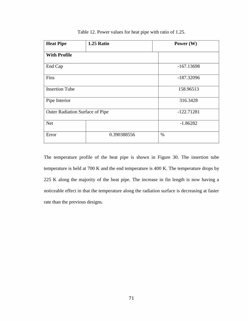
71
Table 12. Power values for heat pipe with ratio of 1.25.
Heat Pipe 1.25 Ratio Power (W)
With Profile
End Cap -167.13698
Fins -187.32096
Insertion Tube 158.96513
Pipe Interior 316.3428
Outer Radiation Surface of Pipe -122.71281
Net -1.86282
Error 0.390388556 %
The temperature profile of the heat pipe is shown in Figure 30. The insertion tube
temperature is held at 700 K and the end temperature is 400 K. The temperature drops by
225 K along the majority of the heat pipe. The increase in fin length is now having a
noticeable effect in that the temperature along the radiation surface is decreasing at faster
rate than the previous designs.

72
Figure 30. Temperature (K) contour of heat pipe with 0.75 fin width to pipe length ratio.
5.3.5 Ratio of 1.5
The outer cylinder consisted of a base circle with a diameter of 25 mm. An inner circle
of 23 mm was created to make a hollow heat pipe. Then end caps of 23 mm in diameter
and 2 mm in thickness were created and the material merged into the existing heat pipe
material. The fins were 37.5 mm in width but 2 mm in thickness due to limitations of the
program and mesh. This was extruded to a length of 300 mm. The schematic of this design
is shown in Figure 31.
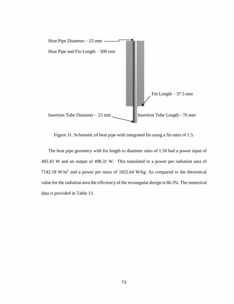
73
Heat Pipe Diameter – 25 mm
Heat Pipe and Fin Length – 300 mm
Fin Length – 37.5 mm
Insertion Tube Diameter – 23 mm Insertion Tube Length - 76 mm
Figure 31. Schematic of heat pipe with integrated fin using a fin ratio of 1.5.
The heat pipe geometry with fin length to diameter ratio of 1.50 had a power input of
492.43 W and an output of 498.31 W. This translated to a power per radiation area of
7142.18 W/m2 and a power per mass of 1822.64 W/kg. As compared to the theoretical
value for the radiation area the efficiency of the rectangular design is 66.3%. The numerical
data is provided in Table 13.

74
Table 13. Power values for heat pipe with ratio of 1.5.
Heat Pipe 1.5 Ratio Power (W)
End Cap -165.90965
Fins -212.78896
Insertion Tube 164.57774
Pipe Interior 332.38892
Outer Radiation Surface of Pipe -119.6151
Net -1.34705
Error 0.270321681 %
The temperature profile of the heat pipe is shown in Figure 32. The insertion tube
temperature is held at 700 K and the end temperature is 400 K. The temperature drops
again by 225 K along the majority of the heat pipe. This design has the most rapid
temperature decrease among the heat pipe designs. This is expected as the increase in fin
size created a larger surface area for radiation.

75
Figure 32. Temperature (K) contour of heat pipe with 1.5 fin width to pipe length ratio.
5.3.6 Results and Discussions of Fin Length Comparison with Profile Data
The following results shown in Figure 33 are the temperature contours of the
simulations comparing fin ratios. From the temperature contour plots it is observed that the
temperature decreases more rapidly as the fin length is increased. This combined with the
increase in mass due to general size demonstrates that a smaller fin length is reasonable
and preferable.

76
(a) (b) (c) (d)
Figure 33. Temperature (K) comparison of various fin lengths and wick profile data. (a)
Heat Pipe (b) Heat Pipe with ratio of 0.5 (c) Heat Pipe with ratio of 1.0 and (d) Heat Pipe
with ratio of 1.5.
The following data in table, Table 14, shows that maximum heat transfer per unit area
and per unit mass occurs at a fin width to pipe diameter of 0.5 ratio. It is also of note that
the efficiency decreases as the width of the fins increase. This decrease in efficiency is
significant, at 32.2 % decrease over the change in fin width, and must be considered. Since
the optimal fin width to pipe diameter is on the lower end the efficiency is nearly 90% thus
the efficiency is higher than would be expected. The power per unit area and power per
unit mass were shown as a function of fin ratio in Figure 34. This data proved somewhat
inconclusive as the values for the ratios of 0.25 and 0.5 were extremely close. For this
reason the data was put into a bar chart to compare power per unit area, shown in Figure
35, and power per unit mass, shown in Figure 36, in order to better compare the data.

77
Table 14. Comparison of power per unit area and power per unit mass for various fin
width to pipe diameter for design including wick profile data.
Geometry Output Area Mass Power/Area
Power/
Mass
Theoretical
Power
Output
Efficiency
(W) m2 kg W/m2 W/kg W %
Heat Pipe 110.38 0.05374 0.9476 2053.96 116.48 578.49 19.08
Heat Pipe
Ratio 0.25 339.36 0.03199 0.1704 10608.32 1991.55 344.36 98.55
Heat Pipe
Ratio 0.50 382.13 0.03956 0.1884 9659.50 2028.29 425.85 89.73
Heat Pipe
Ratio 0.75 406.96 0.04681 0.2088 8693.87 1949.04 503.89 80.76
Heat Pipe
Ratio 1.0 441.76 0.05466 0.2317 8081.96 1906.60 588.39 75.08
Heat Pipe
Ratio 1.25 477.17 0.06222 0.2521 7669.08 1892.78 669.77 71.24
Heat Pipe
Ratio 1.5 498.31 0.06977 0.2734 7142.18 1822.64 751.04 66.35

78
Figure 34. Comparison of power per unit area and power per unit mass for various fin
width to pipe diameter for design including wick profile data.
Figure 35. Power per unit area for various fin ratios for design including wick profile
data.
0.00
2000.00
4000.00
6000.00
8000.00
10000.00
12000.00
0 0.5 1 1.5 2
Po
we
r/A
rea
(W/m
^2)
Length to Diameter Ratio
Heat Pipe Diameter to Fin Length Ratio Comparison
Power/Area
Power/Mass
Power per Unit Area v Fin Length Ratio
Heat Pipe
Heat Pipe with0.25 Ratio
Heat Pipe with0.5 Ratio
Heat Pipe with0.75 Ratio
Heat Pipe with1.0 Ratio
Power /Area (W/m2))

79
Figure 36. Power per unit mass comparison for various fin ratios for design including
wick profile data.
5.4 Heat Pipe Design for Fin Width Comparison without Profile Correction
Another area of interest was how much effect did the wick profile data have on the
ultimate result of the simulation. This was of interest for two reasons. First, it validates that
the equivalent wick performance study was necessary since the wick structure was not
being modeled in this design. Second, it determines if there is a need to at some point
numerically model various wick structures due the impact on the overall design. The same
designs, varying of fin ratios, as above were simulated and power outputs determined.
5.4.1 Heat Pipe with No Fin
The heat pipe geometry no fin had a power input of 1.24 W and an output of 1.24 W.
This translated to a power per radiation area of 23.07 W/m2 and a power per mass of 1.31
0.00
500.00
1000.00
1500.00
2000.00
2500.00
�Power/ Mass (W/kg)
Power per Unit Mass v Fin Length Ratio
Heat Pipe
Heat Pipe with Ratio 0.25
Heat Pipe with Ratio 0.5
Heat Pipe with Ratio 0.75
Heat Pipe with Ratio 1.0
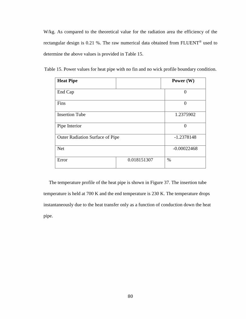
80
W/kg. As compared to the theoretical value for the radiation area the efficiency of the
rectangular design is 0.21 %. The raw numerical data obtained from FLUENT® used to
determine the above values is provided in Table 15.
Table 15. Power values for heat pipe with no fin and no wick profile boundary condition.
Heat Pipe Power (W)
End Cap 0
Fins 0
Insertion Tube 1.2375902
Pipe Interior 0
Outer Radiation Surface of Pipe -1.2378148
Net -0.00022468
Error 0.018151307 %
The temperature profile of the heat pipe is shown in Figure 37. The insertion tube
temperature is held at 700 K and the end temperature is 230 K. The temperature drops
instantaneously due to the heat transfer only as a function of conduction down the heat
pipe.

81
Figure 37. Temperature (K) profile of heat pipe with no fin and no wick profile boundary
condition.
5.4.2 Ratio of 0.25
The heat pipe geometry with fin length to heat pipe diameter ratio of 0.25 had a power
input of 102.02 W and an output of 104.36 W. This translated to a power per radiation
area of 3262.27 W/m2 and a power per mass of 612.44 W/kg. As compared to the
theoretical value for the radiation area the efficiency of the rectangular design is 30.3 %.
The raw numerical data obtained from FLUENT® used to determine the above values is
provided in Table 16.

82
Table 16. Power values for heat pipe with ratio of 0.25 and no wick profile boundary
condition.
Heat Pipe 0.25 Ratio Power (W)
End Cap -0.4727065
Fins -27.491296
Insertion Tube 102.02179
Pipe Interior 0
Outer Radiation Surface of Pipe -76.399496
Net -2.3417085
Error 2.243800307 %
The temperature profile of the heat pipe is shown in Figure 38. The insertion tube
temperature is held at 700 K and the end temperature is 427 K. The temperature drops 220
K along the first half of the heat pipe. This gradient is more gradual than that of the heat
pipe with the working fluid boundary conditions.

83
Figure 38. Temperature (K) profile of heat pipe with 0.25 ratio and no wick profile
boundary condition.
5.4.3 Ratio of 0.5
The heat pipe geometry with fin length to diameter ratio of 0.50 had a power input of
118.15 W and an output of 122.55W. This translated to a power per radiation area of
3097.83 W/m2 and a power per mass of 650.48 W/kg. The raw numerical data obtained
from FLUENT® used to determine the above values is provided in Table 17. As compared
to the theoretical value for the radiation area the efficiency of the rectangular design is 28.8
%.

84
Table 17. Power values for heat pipe with ratio of 0.5 and no wick profile boundary
condition.
Heat Pipe 0.5 Ratio Power (W)
End Cap -0.46094671
Fins -48.857798
Insertion Tube 118.14722
Pipe Interior 0
Outer Radiation Surface of Pipe -73.231041
Net -4.40256571
Error 3.592471161 %
The temperature profile of the heat pipe is shown in Figure 39. The insertion tube
temperature is held at 700 K and the end temperature is 423 K. The temperature drops only
200 K along the heat pipe. The profile is what would be expected of a hollow material.
Since there is no compensation for the wick effect the heat transfer along the heat pipe
behaves much like that of the solid materials. The majority of the heat transfer occurs in
the first two thirds of the heat pipe and the rest of the pipe has a relatively low temperature
causing a decreased temperature gradient.
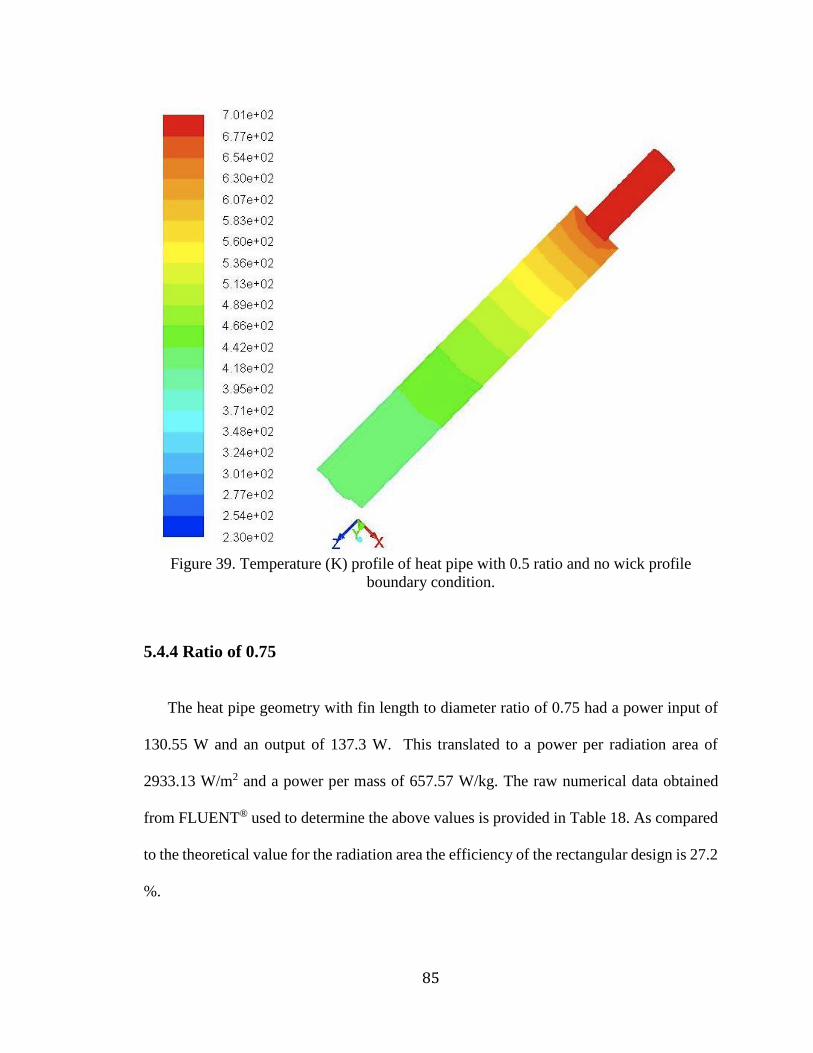
85
Figure 39. Temperature (K) profile of heat pipe with 0.5 ratio and no wick profile
boundary condition.
5.4.4 Ratio of 0.75
The heat pipe geometry with fin length to diameter ratio of 0.75 had a power input of
130.55 W and an output of 137.3 W. This translated to a power per radiation area of
2933.13 W/m2 and a power per mass of 657.57 W/kg. The raw numerical data obtained
from FLUENT® used to determine the above values is provided in Table 18. As compared
to the theoretical value for the radiation area the efficiency of the rectangular design is 27.2
%.

86
Table 18. Power values for heat pipe with ratio of 0.75 and no wick profile boundary
condition.
Heat Pipe 0.75 Ratio Power (W)
End Cap -0.4449315
Fins -65.462685
Insertion Tube 130.54867
Pipe Interior 0
Outer Radiation Surface of Pipe -71.397853
Net -6.7567954
Error 4.920995081 %
The temperature profile of the heat pipe is shown in Figure 40. The insertion tube
temperature is held at 700 K and the end temperature is 419 K. The temperature drops 210
K along the first half of the heat pipe. As the fin length gets longer the end cap temperature
is dropping more rapidly for each case and the area where the temperature is at its lowest
is growing to be a larger portion of the heat pipe.

87
Figure 40. Temperature (K) profile of heat pipe with 0.75 ratio and no wick profile
boundary condition.
5.4.5 Ratio of 1.0
The heat pipe geometry with fin length to heat pipe diameter ratio of 1.0 had a power
input of 144.89 W and an output of 146.95 W. This translated to a power per radiation
area of 1967.80 W/m2 and a power per mass of 464.22W/kg. As compared to the theoretical
value for the radiation area the efficiency of the rectangular design is 18.3%. The raw
numerical data obtained from FLUENT® used to determine the above values is provided
in Table 19.

88
Table 19. Power values for heat pipe with ratio of 1.0 and no wick profile boundary
condition.
Heat Pipe 0.25 Ratio Power (W)
End Cap -0.3925079
Fins -80.260336
Insertion Tube 144.89731
Pipe Interior 0
Outer Radiation Surface of Pipe -66.300562
Net -2.3417085
Error 2.243800307 %
The temperature profile of the heat pipe is shown in Figure 41. The insertion tube
temperature is held at 700 K and the end temperature is 409 K. The temperature drops by
220 K along the majority of the heat pipe.

89
Figure 41. Temperature (K) profile of heat pipe with 1.0 ratio and no wick profile
boundary condition.
5.4.6 Ratio of 1.25
The heat pipe geometry with fin length to diameter ratio of 1.25 had a power input of
155.22 W and an output of 160.50 W. The raw numerical data obtained from FLUENT®
used to determine the above values is provided in Table 20. This translated to a power per
radiation area of 2579.56 W/m2 and a power per mass of 636.65 W/kg. As compared to the
theoretical value for the radiation area the efficiency of the rectangular design is 23.4 %.

90
Table 20. Power values for heat pipe with ratio of 1.25 and no wick profile boundary
condition.
Heat Pipe 1.25 Ratio Power (W)
End Cap -0.039151176
Fins -95.579111
Insertion Tube 155.22203
Pipe Interior 0
Outer Radiation Surface of Pipe -64.884426
Net -5.280658176
Error 3.2900746 %
The temperature profile of the heat pipe is shown in Figure 42. The insertion tube
temperature is held at 700 K and the end temperature is 407 K. The majority of the
temperature drop occurs in the first third of the heat pipe. This leaves a large portion of the
pipe and fin at a relatively low temperature.

91
Figure 42. Temperature (K) profile of heat pipe with 1.25 ratio and no wick profile
boundary condition.
5.4.7 Ratio of 1.5
The heat pipe geometry with fin length to diameter ratio of 1.50 had a power input of
164.0 W and an output of 169.84 W. This translated to a power per radiation area of
2434.28 W/m2 and a power per mass of 621.21 W/kg. As compared to the theoretical value
for the radiation area the efficiency of the rectangular design is 22.6 %. The raw numerical
data obtained from FLUENT® used to determine the above values is provided in Table 21.

92
Table 21. Power values for heat pipe with ratio of 1.5 and no wick profile boundary
condition.
Heat Pipe 1.5 Ratio Power (W)
End Cap -0.37258853
Fins -107.08915
Insertion Tube 163.96104
Pipe Interior 0
Outer Radiation Surface of Pipe -62.380008
Net -5.88070653
Error 3.462462351 %
The temperature profile of the heat pipe is shown in Figure 43. The insertion tube
temperature is held at 700 K and the end temperature is 402 K. The temperature drops 200
K in the first quarter of the heat pipe. This leaves the majority of the heat pipe operating at
a lower temperature than other designs.
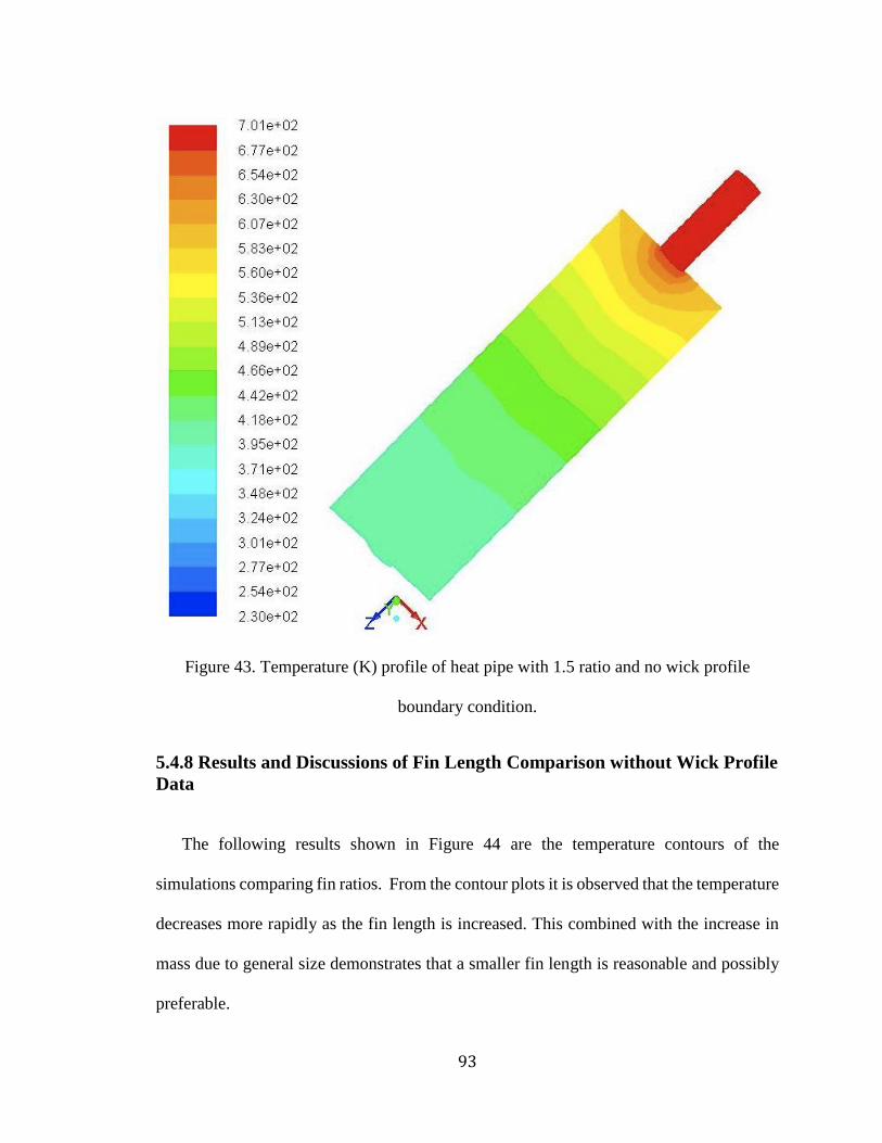
93
Figure 43. Temperature (K) profile of heat pipe with 1.5 ratio and no wick profile
boundary condition.
5.4.8 Results and Discussions of Fin Length Comparison without Wick Profile
Data
The following results shown in Figure 44 are the temperature contours of the
simulations comparing fin ratios. From the contour plots it is observed that the temperature
decreases more rapidly as the fin length is increased. This combined with the increase in
mass due to general size demonstrates that a smaller fin length is reasonable and possibly
preferable.

94
(a) (b) (c) (d)
Figure 44. Temperature comparison of various fin widths and no wick profile boundary
condition. (a) Heat Pipe (b) Heat Pipe with ratio of 0.5 (c) Heat Pipe with ratio of 1.0 and
(d) Heat Pipe with ratio of 1.5
The following data in Table 22 shows that maximum heat transfer per unit area and per
unit mass occurs at a fin width to pipe diameter of 0.5 ratio. It is also of note that the
efficiency decreases as the width of the fins increase. This decrease in efficiency,
approximately 7%, is negligible and thus not a primary concern in determining the best fin
width to pipe length ratio.
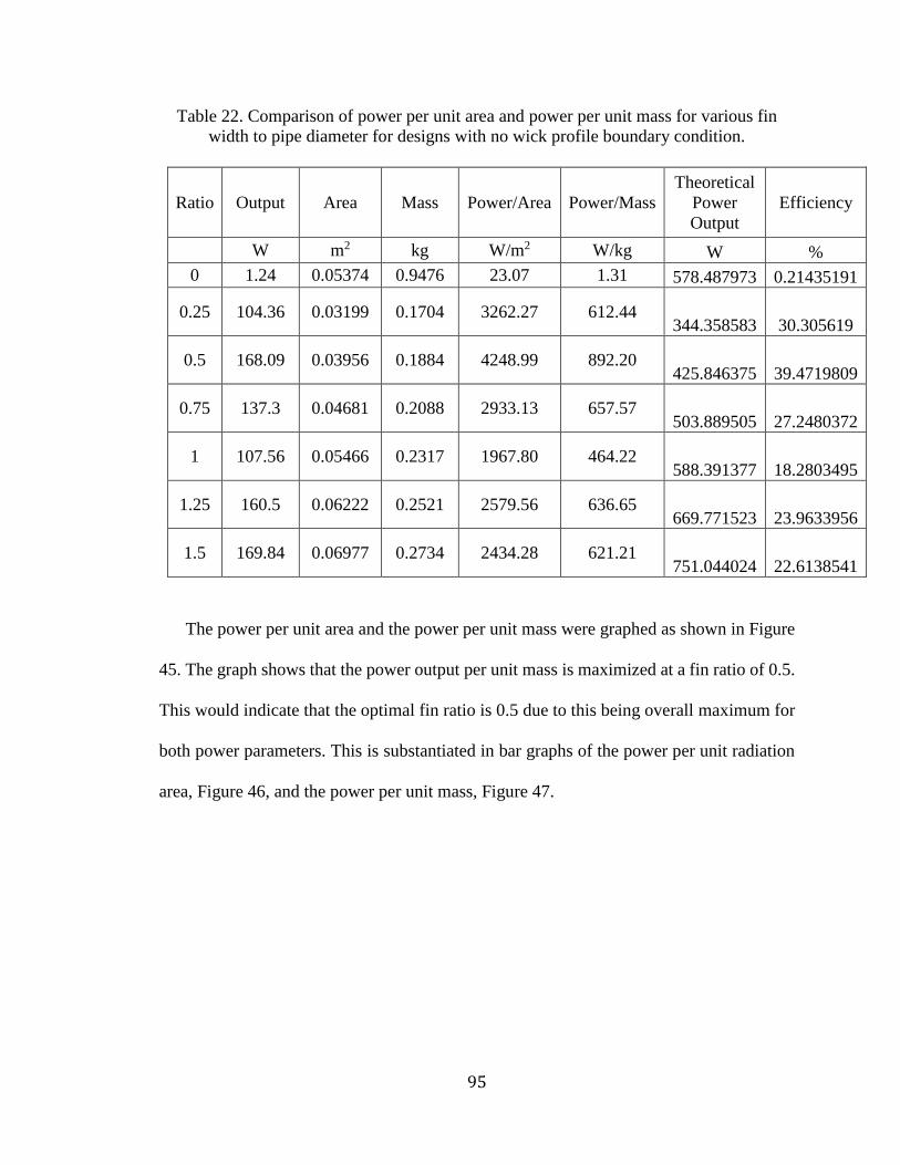
95
Table 22. Comparison of power per unit area and power per unit mass for various fin
width to pipe diameter for designs with no wick profile boundary condition.
Ratio Output Area Mass Power/Area Power/Mass
Theoretical
Power
Output
Efficiency
W m2 kg W/m2 W/kg W %
0 1.24 0.05374 0.9476 23.07 1.31 578.487973 0.21435191
0.25 104.36 0.03199 0.1704 3262.27 612.44 344.358583 30.305619
0.5 168.09 0.03956 0.1884 4248.99 892.20 425.846375 39.4719809
0.75 137.3 0.04681 0.2088 2933.13 657.57 503.889505 27.2480372
1 107.56 0.05466 0.2317 1967.80 464.22 588.391377 18.2803495
1.25 160.5 0.06222 0.2521 2579.56 636.65 669.771523 23.9633956
1.5 169.84 0.06977 0.2734 2434.28 621.21 751.044024 22.6138541
The power per unit area and the power per unit mass were graphed as shown in Figure
45. The graph shows that the power output per unit mass is maximized at a fin ratio of 0.5.
This would indicate that the optimal fin ratio is 0.5 due to this being overall maximum for
both power parameters. This is substantiated in bar graphs of the power per unit radiation
area, Figure 46, and the power per unit mass, Figure 47.

96
Figure 45. Comparison of power per unit area and power per unit mass for various fin
width to pipe diameter for designs with no wick profile boundary condition.
Figure 46. Power per unit area for various fin ratios for design with no wick profile
boundary condition.
0.00
500.00
1000.00
1500.00
2000.00
2500.00
3000.00
3500.00
4000.00
4500.00
0 0.5 1 1.5 2
Ratio
Heat Pipe Diameter to Fin Length Ratio Comparison
Power/Area
Power/Mass
0.00
500.00
1000.00
1500.00
2000.00
2500.00
3000.00
3500.00
4000.00
4500.00
Power/Area (W/m^2)
Power per Unit Area v Fin Length Ratio
Heat Pipe
Heat Pipe with Ratio 0.25
Heat Pipe with Ratio 0.5
Heat Pipe with Ratio 0.75
Heat Pipe with Ratio 1.0
Heat Pipe with Ratio 1.25
Heat Pipe with Ratio 1.5

97
Figure 47. Power per unit mass comparison for various fin ratios for with no wick profile
boundary condition.
5.5 Comparison of Non-Wick Effect Trials and Wick Effect Trials
The temperature of the exterior of each heat pipe was exported into Excel.
Using Excel, the axial external heat pipe temperature was plotted and compared to the
expected profile for both the wick performance study and the benchmark study. The
results of this analysis are shown below.
0.00
100.00
200.00
300.00
400.00
500.00
600.00
700.00
800.00
900.00
1000.00
Power/Mass (W/kg)
Power per Unit Mass v Fin Length Ratio
Heat Pipe
Heat Pipe with Ratio 0.25
Heat Pipe with Ratio 0.5
Heat Pipe with Ratio 0.75
Heat Pipe with Ratio 1.0
Heat Pipe with Ratio 1.25
Heat Pipe with Ratio 1.5

98
Figure 48. Comparison of power per unit area and power per unit mass for various fin
width to pipe diameter with no interior temperature profile.
The het pipe temperature profiles represented in Figure 48 were determined to be
lacking because of the failure to take internal wick effects into consideration in the model.
The temperature profile drops quickly, similar to that of the solid geometries, since all the
effects are those of conduction and radiation. For this reason the pipe interior was modeled
with a simulated wick performance. This boundary condition takes into account the
convection that occurs in the working fluid. In doing this, the efficiency increases to that
of the Juhasz’s (1998) design. The temperature profile also changes to mimic that of the
flight test data found in Chapter 4. By including the interior fluid effects the operating

99
temperature along the heat pipe is increased to a steady temperature around 600K. The
external heat pipe temperatures using the wick profile information are provided below in
Figure 49. These are consistent with both the wick study and the flight test data.
Figure 49. Comparison of power per unit area and power per unit mass for various fin
width to pipe diameter with an interior temperature profile.

100
Chapter 6
Conclusions A series of various geometries of solid fins and heat pipes with and without fins were
modeled using FLUENT. The general heat pipe design consisted of a heat pipe with a 25
mm outer diameter, 23 mm inner diameter, and was 300 mm in length. Fin sizes ranged
from 6.25 mm to 37.5 mm in length. Using the power output per unit area and power output
per unit mass, to verify that a heat pipe was the best selection for a lunar radiator system.
The parametric study returned the expected results that the heat pipe provided the
highest power output for both the mass and radiation area. The heat pipe design is
superior to the solid geometries that were considered. The heat pipe was lighter and
had the same radiation area. The heat pipe was able to radiate more heat that it’s
solid counterparts as well.
The heat pipe with integrated fin design outperformed the standard heat pipe. The
fin allowed the length to be decreased by over half and also reduced the mass of the
pipe. It also provided higher power transfer out of the system.
The heat pipe with a fin ratio of 0.5, 12.5 mm, was the best performing design when
the effect of the wick was not taken into account. It produced the highest power
output for both mass and area. However, this did not accurately describe the
realistic operation of the heat pipe.
The heat pipe with a fin ratio of 0.5 was the best performer when the wick profile
was applied. The 0.25 fin ratio design provided better efficiency and heat transfer
per unit area; however, the 0.5 fin ratio performed nearly as well and had a slight

101
advantage in the power output per unit mass. This improved performance, 34.47
W/kg, could translate into nearly 5 kW increase for a radiator system containing
138 finned heat pipes. This coupled with the reduced mass, a major consideration
for space systems, drove the decision to select the 0.5 fin ratio as the optimal design.
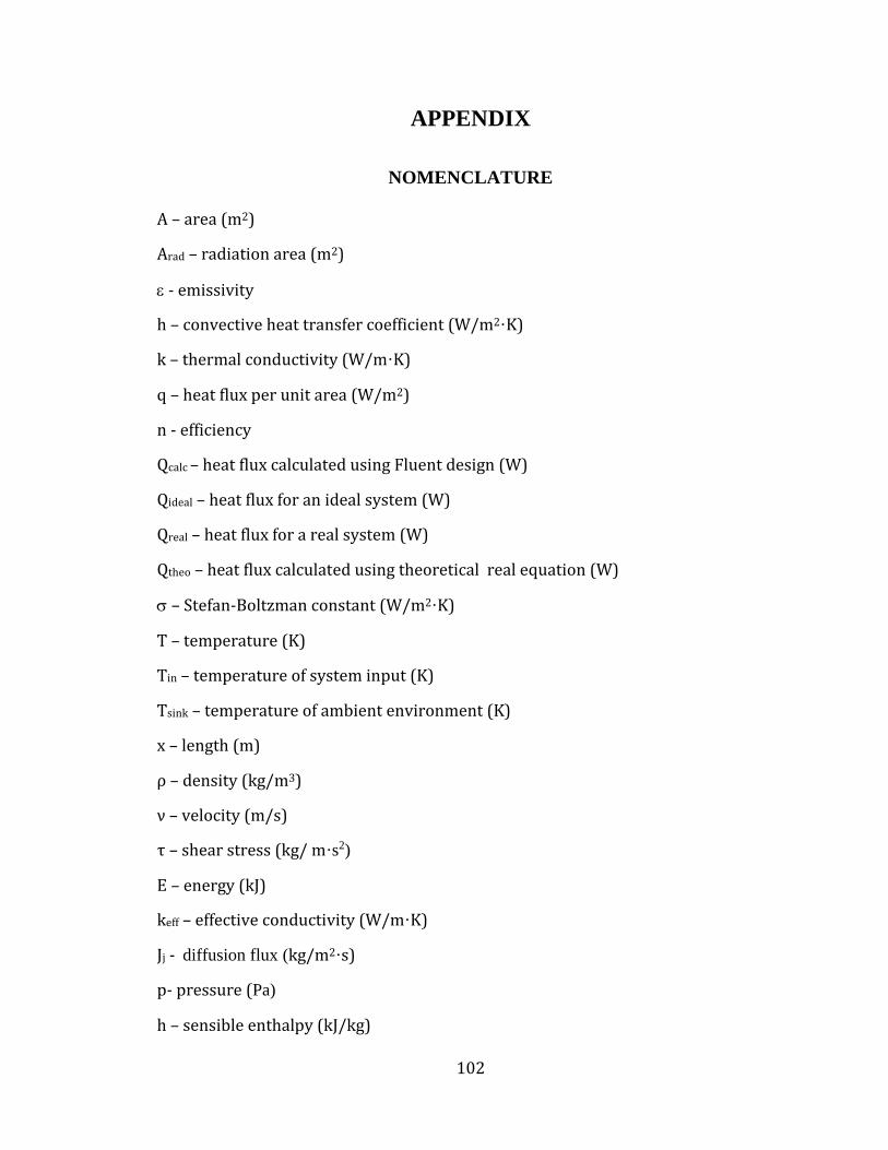
102
APPENDIX
NOMENCLATURE A – area (m2)
Arad – radiation area (m2)
- emissivity
h – convective heat transfer coefficient (W/m2·K)
k – thermal conductivity (W/m·K)
q – heat flux per unit area (W/m2)
n - efficiency
Qcalc – heat flux calculated using Fluent design (W)
Qideal – heat flux for an ideal system (W)
Qreal – heat flux for a real system (W)
Qtheo – heat flux calculated using theoretical real equation (W)
– Stefan-Boltzman constant (W/m2·K)
T – temperature (K)
Tin – temperature of system input (K)
Tsink – temperature of ambient environment (K)
x – length (m)
ρ – density (kg/m3)
ν – velocity (m/s)
τ – shear stress (kg/ m·s2)
E – energy (kJ)
keff – effective conductivity (W/m·K)
Jj - diffusion flux (kg/m2·s)
p- pressure (Pa)
h – sensible enthalpy (kJ/kg)

103
Yj- mass fraction the component that is in the gas form
cp – specific heat at constant pressure (kJ/kg·K)
Sh – energy added by chemical reaction and other volumetric heat sources (kJ)
Sm – mass added to the continuous phase from the dispersed second phase (kg)
g –gravity (m/s2)
F – external force (kg·m/s2)

104
References 1. Antoniak, Z.I., Webb, B. J., and Bates, J. M., 1991, “Testing of Advanced Ceramic
Fabric Heat Pipe for a Stirling Engine,” AIAA/NASA/OAI Conference on Advanced
SEI Technologies, Cleveland, Ohio.
2. Arslanturk , C., 2005, “Optimum Design of Space Radiators with Temperature-
Dependent Thermal Conductivity,” Applied Thermal Engineering 26 (1149–1157)
3. Belvin, W.K., Watson, J.J., and Singhal, S.N., 2006, “Structural Concepts and
Materials for Lunar Exploration Habitats,” American Institute of Aeronautics and
Astronautics, Space 2006, San Jose, CA.
4. Bowman, W.J., and Maynes, D., 2001, “Comparaison of Standard and Heat-Pipe
Fins with Specified Tip Temperature Condition,” Journal of Thermophysics and Heat
Transfer Vol.15 No.4 (421-426), doi: 10.2514/2.6645
5. Bowman, W. J., Moss, T. W., Maynes, D., and Paulson, K. A., 1999, “Efficiency of a
Constant-Area, Adiabatic Tip, Heat Pipe Fin,” J. Thermophysics, Vol. 14, No.
1:Technical Notes (112-115), doi: 10.2514/2.6497
6. Bowman, W.J., Storey, J.K. and Svensson, K.I., 1999, “Analytical Comparison of
Constant Area, Adiabatic Tip, Standard Fins, and Heat Pipe Fins,” Journal of
Thermophysics and Heat Transfer Vol.13 No.2 (269-272), doi: 10.2514/2.6432
7. Brandhorst , H.W. and Rodiek, J.A., 2006, “A Liquid Sheet Radiator for a Lunar
Stirling Power System,” Space Research Institute, Auburn University, Auburn
University, AL 36849-5320
8. Diwekar, U.M. and Morel, B., 1993, “Space Nuclear Power Plants – I,” Computers
and Chemical Engineering, Vol. 17 No.9, pp 873-878
9. Elliott, J.O., Lipinski, R.J., And Poston, D.I., 2003, “Design Concept for a Nuclear
Reactor-Powered Mars Rover,” Space Technology and Application International
Forum (STAIF 2003) Albuquerque, NM, USA
10. Faghri, Amir, 1995, Heat Pipe Science And Technology. Taylor & Francis Group.
ISBN 978-1560323839
11. Ganapathi, G.B., Birur, G.C., Tsuyuki, G.T., McGrath, P.L. and Patzold, J.D., 2003,
“Active Heat Rejection System on Mars Exploration Rover - Design Changes from
Mars Pathfinder,” AIP Conf. Proc., Volume 654, pp. 206-217
12. Incropera, F.P. and DeWitt, D.P., 1996, Fundamentals of Heat and Mass Transfer,
John Wiley & Sons, Inc. 4th edition (110-130 and 634-754)
13. Juhasz, A.J., 1998, “Design Considerations for Lightweight Space Radiators Based
on Fabrication and Test Experience With a Carbon-Carbon Composite Prototype Heat
Pipe,” National Aeronautics and Space Administration, Glenn Research Center,
Cleveland, Ohio 44135
14. Juhasz, A.J., 2001, “Mathematical Analysis of Space Radiator Segmenting for
Increased Reliability and Reduced Mass,” National Aeronautics and Space
Administration, Glenn Research Center, Cleveland, Ohio 44135
http://ntrs.nasa.gov/archive/nasa/casi.ntrs.nasa.gov/20010069503_2001112709.pdf.
15. Juhasz, A.J., 2007, “Heat Transfer Analysis of a Closed Brayton Cycle Space
Radiator.,” National Aeronautics and Space Administration, Glenn Research Center,
Cleveland, Ohio 44135

105
16. Juhasz, A.J., Tew, R.C., Thieme, L.G., 2000, “Parametric Study of Radiator Concepts
for Stirling Radioisotope Power System Applicable to Deep Space Missions,”
National Aeronautics and Space Administration, Glenn Research Center, Cleveland,
Ohio 44135
http://gltrs.grc.nasa.gov/reports/2000/TP-2000-209676.pdf.
17. Keddy
18. Klein, A.C., Al-Baroudi, H., Gulshan-Ara, Z., Kiestler, W.C., Snuggerud, R.D.,
Abdul-Hamid, S.A., and Marks, T.S., 1993, “Fabric Composite Radiators for Space
Nuclear Power Applications. Final Report,” Oregon State Univ., Corvallis, OR
(United States). Dept. of Nuclear Engineering
DOI: 10.2172/106730
19. Krikkis, R.N. and Razelos, P., 2002, “Optimum Design of Spacecraft Radiators With
Longitudinal Rectangular and Triangular Fins,” Journal of Heat Transfer October
2002, Vol. 124 (805-811).
20. Krishnaprakas, C.K. and Narayana, K.B., 2003, “Heat transfer analysis of mutually
irradiating fins,” International Journal of Heat and Mass Transfer 46 (761–769), doi:
10.1016/S0017-9310(02)00356-3 .
21. Mattick, A.T. and Hertzberg, A., 1981, “Liquid Droplet Radiators for Heat Rejection
in Space,” Journal Energy, Vol. 5, No. 6.
22. Mattick, A.T. and Hertzberg, A., 1985, “Liquid Droplet Radiator Performance
Studies,” Acta Astronautica Vol. 12, No. 7/8, pp. 591-598
23. Naumann, R.J., 2004, “Optimizing the Design of Space Radiators,” International
Journal of Thermophysics, Vol. 25, No. 6
24. Nelson, G, 2007, “Liquid Droplet Space Radiator,” University of California, San
Deigo, MAE221A – Heat Transfer
25. Pfeiffer, S.L., 1989, “Conceptual Design of Liquid Droplet Radiator
Shuttle-Attached Experiment,” Grumman Space Systems, Bethpage, New York
26. Roy, S.K. and Avanic, B.L., 2006, “Optimization of a Space Radiator with Energy
Storage.” International Communications in Heat and Mass Transfer, Vol. 33 iss: 5
27. Ruess, F. Schaenzlin, J. and Benaroya, H., 2006, “Structural Design of a Lunar
Habitat,” Journal of Aerospace Engineering, Vol. 19 No. 3
28. Siamidis, J., 2006, “Heat Rejection Concepts for Lunar Fission Surface Power
Applications,” Analex Corporation, Brook Park, Ohio, NASA/CR—2006-214388
29. Tagliafico, L.A. and Fossa,, M., 1997, “Lightweight radiator optimization for heat
rejection in space,” Heat and Mass Transfer 32 (239–244)
30. Tagliafico, L.A. and Fossa,, M., 1999, “Liquid Sheet Radiators for Space Power
Systems,” Proceedings of the Institution of Mechanical Engineers. Part G, Journal of
aerospace engineering [0954-4100] vol: 213 iss:6 pg:399 -406
DOI: 10.1243/0954410991533115
31. Teti, N., 2002, “Carbon-Carbon Radiator Validation Report”, Swales Aerospace,
Beltsville, Maryland 20705
http://eo1.gsfc.nasa.gov/new/validationreport/Technology/Documents/Reports/CCR.p
df
32. Vaughn, W., Shinn, E., Rawal, S., and Wright, J., 1998, “Carbon-Carbon Composite
Radiator Development for the EO-1 Spacecraft”, Technical Report, NASA Langley
Technical Report Server

106
http://www.acm-nevada.com/Technical/Radiator%20C-C.pdf
33.Woloshun, K.A. Merrigan, M.A., Sena, J.T., Secary, J., “High Temperature Heat Pipe
Experiments Aboard the Space Shuttle.” AIP Conf. Proc. 271, pp. 523-531

107
VITA
Graduate College University of Nevada, Las Vegas
Virginia Ruth Bieger
Local Address: 10146 Ragdoll Ave. Las Vegas, Nevada 89166 Degree: Bachelor of Science, Chemical Engineering Louisiana Tech University Publications: Virginia R. Bieger, Jian Ma, Investigation of Lightweight Space Radiator Design for Low and No Gravity Environments, Proceedings of the ASME 2011 International Mechanical Engineering Congress & Exposition, 2011, Denver, Colorado, USA, November 2011 Thesis Title: Numerical Modeling of Heat Pipe Radiator Thesis Examination Committee: Chairperson: Yitung Chen. Ph.D. Committee Member: Robert F. Boehm, Ph.D. Committee Member: Hui Zhao, Ph.D. Committee Member: Jian Ma, Ph.D. Graduate Faculty Representative: Yingtao Jiang, Ph.D.